Renewable Energy Policy Alternatives for the Future

Wallace E. Tyner and Farzad Taheripour1

The United States has been subsidizing ethanol since 1978. In the last decade, a subsidy

has been added for biodiesel. The ethanol subsidy has ranged from 40 to 60 cents per

gallon over the entire time period (Tyner and Taheripour, 2007). The ethanol subsidy is

currently 51 cents per gallon, and the biodiesel subsidy is 50 cents for biodiesel made

from recycled materials such as cooking grease or tallow and $1 per gallon for biodiesel

made from oilseed crops, such as soybeans. Over the years the objectives for biofuel

subsidies have included increased farm income, achieving environmental gains (clean

burning), increasing national security, and more recently reducing greenhouse gas (GHG)

emissions related to global warming. At present, the national security objective seems to

be the top priority (Copulos, 2003 and 2007).

Crude oil price as measured by U.S. refinery acquisition cost in nominal terms has

ranged between $10 and $30/bbl between 1978 and 2004, except for a couple of short

term spikes (see figure 1). Thus, for most of the period we have had a fixed ethanol

subsidy, while the crude oil price has been around $20/bbl. In 2004, the crude oil price

began its steep climb to around $70/bbl, and it has been hovering around $60/bbl in

recent months. This rapid increase in the crude price while the ethanol subsidy remained

fixed led to a tremendous boom in construction of ethanol plants. Ethanol production in

2005 was about 4 billion gallons, and it will be 8 billion in 2007, and surpass 11 billion in

Tyner and Taheripour are Professor and Post-doc, Department of Agricultural

Economics, Purdue University.

2

2008. It has been, then, the combination of high oil prices and a subsidy that was keyed

to $20 oil that has led to this boom. The ethanol boom has, in turn, led to a rapid run-up

in corn and other commodity prices (soybeans and wheat, in particular) in 2006-07. The

run-up in commodity prices has fueled debate over the food-fuel issue and raised

questions on the extent to which renewable fuels can be supplied from corn alone.

These debates have also led to discussions of alternative mechanisms for

stimulating renewable fuels production. In this article, we examine some other

alternatives and their likely consequences. Before progressing to other alternatives, it

may be useful to illustrate the impacts of the current policy and its impact on commodity

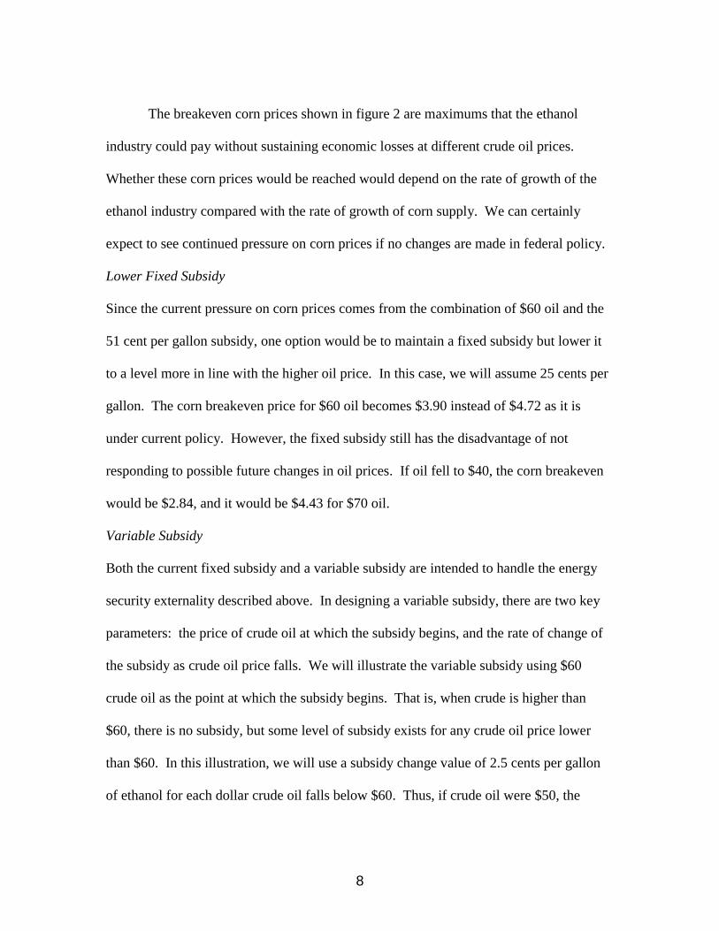
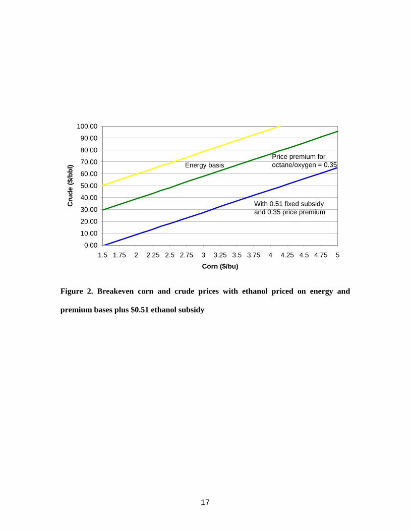
prices. There are three components to the market value of ethanol: energy, additive, and

subsidy. It is interesting to portray these values in terms of the relationship between

crude oil price and the maximum price a dry mill could afford to pay for corn at each

crude oil price. Many assumptions are required to establish these relationships, which are

detailed in Tyner and Taheripour (2007). Figure 2 displays the relationships between

crude oil and breakeven corn prices on the basis of energy equivalence, energy

equivalence plus additive value (the value as an oxygenate is assumed to be 35 cents per

gallon for this illustration), and energy equivalence plus additive value plus the current

federal blending subsidy of 51 cents per gallon. The energy equivalence line is based on

the assumption that ethanol has 70 percent of the energy of gasoline, slightly more than

the direct energy equivalence. Using figure 2, we can trace out the breakeven corn price

for any given crude oil price. For example, with crude oil at $60/bbl, the breakeven corn

price is $4.72/bu including both the additive premium and the fixed federal subsidy.

3

Without the subsidy, the breakeven corn price would be $3.12. These figures are for a

new plant and include 12 percent return on equity and 8 percent debt interest. If we

consider an existing plant with capital already recovered, we add 78 cents per bushel to

yield a breakeven corn price of $5.50. It is important to note that additive value is

currently 20 cents higher than the value assumed here, but this high level is not likely to

persist.

Theoretical Background

Before moving to an analysis of policy alternatives for the future, we provide a

theoretical framework for renewable energy subsidies. The economic theory mainly

elucidates that in the presence of externalities, the government can restore the economic

efficiency using tax and subsidy policies (Baumol and Oates 1988). Although tax and

subsidy policies are well-know policy instruments for dealing with externalities, there are

other alternatives such as alternative fuel standards and cap and trade as well (Bamoul

and Oates, 1988; Goulder et al., 1999; Parry, 2002). In this analysis, we consider only

subsidies and renewable fuels standards. In the U.S. today, the major externalities often

mentioned in the context of renewable fuels are national security and the global warming

associated with greenhouse gas (GHG) emissions. The national security externality

derives from the notion that the U.S. is much less secure as a nation being dependent on

imported oil for almost two-thirds of our supply, with about half of that coming from

sources that are considered to be politically unstable or unreliable. Converting to

domestically-supplied renewable sources is considered to be an important means of

lowering this security cost. The GHG externality related to global warming is linked to

4

renewable fuels because their contribution to GHG emissions is much lower than fossil

fuels, especially renewable fuels from cellulosic materials. In developing the theoretical

model, we consider these two dimensions.

For the theoretical model we assume there are two firms that can produce a

homogeneous liquid biofuel. The first firm (A) produces liquid biofuel from food crops

such as corn. The second firm (B) produces liquid biofuel from cellulosic materials. We

define the following long run cost functions for these firms:

(1) ),( AAAA qxCC =

(2) ),( BBBB qxCC = .

Here CA and CB represent costs for firms A and B; xA and xB are vectors of inputs prices;

and qA and qB represent firms’ outputs. Both firms use primary and intermediate inputs

such as capital, labor, energy, water, and chemicals. In addition, the firm A uses corn, and

the firm B uses cellulosic materials. We assume that the cost structures of these firms are

different, and they have different marginal costs (MC), such that: )()( AABB qMCqMC >

for all values of AB qq = . This means that producing liquid fuel from cellulosic materials

is more expensive than producing liquid fuel from food crops. Assume that the price of

the liquid biofuel P is an increasing function of the price of crud oil Po and that firms are

price takers.

Now suppose production of liquid fuel generates two types of social benefits:

environmental benefits (E) and national security (N). The environmental benefits can be a

reduction in GHG emissions, and the national security benefits can be less dependency on

volatile crude oil imports. In addition, assume that firms are homogeneous in their

5

impacts on national security, but they are heterogeneous in terms of environmental

benefits. We assume that firm B generates higher marginal environmental benefits than

firm A, but both firms have the same marginal national security benefits. To avoid

complexity, suppose E and N are linear homogenous functions in variable q. These

assumptions imply that:

(3) iii qE α= for i = A, B and AB αα > ,

(4) ii qN β= for i = A, B.

Here iα and β denote the environmental and security marginal benefits, respectively.

Now assume that the government wants to correct the market failure due to the existence

of these external benefits. What are the optimal levels of production for these firms? To

answer this question we define the following optimization model for given input prices of

xA and xB:

(5) [ ]∑=

−++=BAi

iiiiiiioqq

qxCqqqPPMaxBA ,,

),()).(( βαπ

The following first-order conditions would determine the optimal production levels in the

presence of external benefits:1

(6) ),()( iiiio qxMCPP =++ βα , for i=A and B.

We denote the potential optimal production levels with *Aq and *

Bq . We consider two

options to achieve these production levels: a subsidy or a renewable fuel standard.

Option 1 – Subsidy

To achieve *Aq and *

Bq the following subsidies should be paid to firms A and B:

(7) iiSE α= , for i=A and B,

6

(8) β=iSN , for i=A and B.

Here SEi and SNi are subsidies per unit of output to correct for environmental and security

benefits, respectively. Indeed, in the presence of environmental and security benefits, the

government should pay two types of subsidies: 1) a subsidy to correct for environmental

benefits and 2) a subsidy for more energy security. We can combine these two subsidies

to define the following subsidy rates: βα += AAS and βα += BBS . With these

subsidies, the firms will chose to produce *Aq and *

Bq . Now since we assume that

AB αα > but both firms have the same marginal national security benefits, the government

should consider a higher total subsidy per unit of output for firm B, AB SS > . This implies

that a uniform subsidy is not an optimal policy when firms’ marginal environmental

benefits are not the same. Indeed, producing liquid biofuel from cellulosic materials

should be supported at a higher level according to the difference in GHG emissions

reductions.

Option 2. Standard

The government can announce ***BA qqq += as the goal for liquid biofuel production and

force it through a penalty system. If the government announces *q for the standard, since

firm A has cost advantages, it will produce more than *Aq and firm B will produce less

than *Bq . In this case while the government can achieve the goal of *q , firms will not

produce at the levels which are socially optimal. To achieve *Aq and *

Bq , the government

needs to announce two levels for standards – the total standard must be partitioned

between the two sources.

7

Future Policy Alternatives

In essence, there is an unintended consequence of the fixed ethanol subsidy. When it was

created, no one envisioned $60 crude oil, but today $60 oil is a reality, and many believe

oil prices are likely to remain high. Given this reality, what future federal policy options

could be considered? There are several possible options:

• Make no changes in the current subsidy system, and let the other corn-using

sectors (particularly livestock) adjust as needed.

• Keep the subsidy fixed. but reduce it to a level more in line with crude oil prices

around $60.

• Convert the subsidy from a fixed subsidy to one that varies with the price of oil.

• Construct a subsidy policy with two components: 1) a national security

component (either fixed or variable) tied to energy content of the fuel, and 2) a

component tied to GHG emissions reductions of the liquid fuel.

• Use an alternative fuel standard instead of subsidies to stimulate growth in

production and use of alternative fuels.

• Use a combination of an alternative fuel standard and a variable subsidy.

No Changes

Certainly, one option is to do nothing – to let the other corn-using sectors adjust to higher

corn prices. But as shown by the results presented above, that option could lead to

substantially higher corn prices than we have seen historically. It certainly would lead to

higher costs for the livestock industry (as currently evidenced) and ultimately for

consumers of livestock products. It also would lead to reduced corn exports.

8

The breakeven corn prices shown in figure 2 are maximums that the ethanol

industry could pay without sustaining economic losses at different crude oil prices.

Whether these corn prices would be reached would depend on the rate of growth of the

ethanol industry compared with the rate of growth of corn supply. We can certainly

expect to see continued pressure on corn prices if no changes are made in federal policy.

Lower Fixed Subsidy

Since the current pressure on corn prices comes from the combination of $60 oil and the

51 cent per gallon subsidy, one option would be to maintain a fixed subsidy but lower it

to a level more in line with the higher oil price. In this case, we will assume 25 cents per

gallon. The corn breakeven price for $60 oil becomes $3.90 instead of $4.72 as it is

under current policy. However, the fixed subsidy still has the disadvantage of not

responding to possible future changes in oil prices. If oil fell to $40, the corn breakeven

would be $2.84, and it would be $4.43 for $70 oil.

Variable Subsidy

Both the current fixed subsidy and a variable subsidy are intended to handle the energy

security externality described above. In designing a variable subsidy, there are two key

parameters: the price of crude oil at which the subsidy begins, and the rate of change of

the subsidy as crude oil price falls. We will illustrate the variable subsidy using $60

crude oil as the point at which the subsidy begins. That is, when crude is higher than

$60, there is no subsidy, but some level of subsidy exists for any crude oil price lower

than $60. In this illustration, we will use a subsidy change value of 2.5 cents per gallon

of ethanol for each dollar crude oil falls below $60. Thus, if crude oil were $50, the

9

subsidy per gallon of ethanol would be 25 cents. If crude oil were $40, the ethanol

subsidy would be 50 cents per gallon. Therefore, for any crude oil price above $40, the

ethanol subsidy would be lower than the current fixed subsidy. For any crude price less

than $40, the subsidy would be greater than the current fixed subsidy.

Figure 3 illustrates the corn breakeven price for different crude oil prices if this

variable subsidy were in effect. In this case, the corn breakeven price at $60 oil for a new

ethanol plant would be $3.12 per bushel, compared to $4.72 with the fixed subsidy shown

in Figure 2. With oil at $50, the corn breakeven would be $2.90 for a new plant with the

variable subsidy. An oil price of $40 would support a corn price of $2.69 for a new plant

and $3.47 for an existing plant with capital recovered. An oil price of $70 would yield a

breakeven corn price of $3.65 with no ethanol subsidy. Thus, the variable subsidy

provides a safety net for ethanol producers without exerting inordinate pressure on corn

prices.

For any crude oil price above $60, there would be no ethanol subsidy with the

variable subsidy; so ethanol plant investment decisions would be made based on market

forces alone instead of being driven by the federal subsidy. For any crude price between

$40 and $60, the variable subsidy would be less than the current fixed subsidy, providing

less incentive to invest and less pressure on corn prices, but maintaining a safety net.

Two-part Subsidy

The two-part subsidy derives directly from the theoretical model provided above. For

this illustration, we construct the national security part of the subsidy based on the energy

content of the renewable fuel. Thus, ethanol from corn or cellulose would have the same

10

energy security subsidy since they have the same energy content, but biodiesel would

have an energy security subsidy 1.5 times larger since it has 150% of the energy content

of ethanol. Similarly, biodiesel would have a larger GHG reduction component than corn

ethanol but lower than cellulose ethanol because of the differences in emissions. The

GHG component would be invariant with the price of crude oil, but the energy security

part could be fixed or variable. In this illustration, we will assume that it is fixed.

Hill et al. (2006) indicate that corn-based ethanol provides a 12.4% reduction in

GHG (compared to gasoline), and soy biodiesel provides a 40.5% reduction (compared to

diesel). Tilman, Hill, and Lehman (2006) suggest that switchgrass can actually be

carbon-negative; that is, more carbon is sequestered than is released in combustion. For

cellulose ethanol, they calculate a 275% reduction in CO2 emissions relative to gasoline

from crude oil. Actual carbon balance depends on the production conditions. For

purposes of this illustration, we will assume that cellulosic ethanol yields a 200% GHG

reduction. One could envision a GHG component of the subsidy keyed to an index. For

simplicity, we will use these three percentage figures for the index values for corn

ethanol, soy biodiesel and cellulose ethanol, respectively.

For the energy security component, we will key it to energy value – that is, to the

energy content of oil displaced. The two-part subsidy is illustrated in figure 4. For this

illustration, we keyed the base values for the national security component and GHG

component to yield a corn ethanol subsidy roughly equivalent to the current federal

ethanol subsidy of 51 cents. The base assumptions are 75 cents for the national security

component per gallon of gasoline equivalent and 25 cents per gallon for 100 percent

11

GHG emissions reduction.2 The resulting total subsidy values are 53 cents for corn

ethanol, 85 cents for soy diesel, and $1.00 for cellulose ethanol. Clearly, these values are

merely illustrative to demonstrate that a two-part subsidy encompassing both the national

security and GHG emissions externalities would be possible to accomplish.

Alternative Fuel Standard

In his 2007 State of the Union message, President Bush proposed a relatively large

alternative fuel standard of 35 billion gallons by 2017. That is roughly seven times

current ethanol production. The Senate has passed a similar proposal. A fuel standard

works very differently from a subsidy. It says the industry must acquire a certain

percentage of its fuel from alternative domestic sources. In the President’s proposal, the

sources could be renewable fuels, clean coal liquids or other domestic sources. With a

fuel standard that is perceived to be iron-clad, the industry is required to procure these

alternative fuels no matter what their cost in the market. Most of the change in cost of

the fuels is passed on to consumers either through cheaper or more expensive fuel at the

pump.3 In other words, if crude oil is much cheaper than alternative fuels, consumers

would pay more at the pump than they would in the absence of the standard. If it turns

out in the future that alternative fuels are less expensive than crude oil, consumers would

actually pay less at the pump. Thus, an alternative fuel standard may be viewed as a

different form of variable subsidy – one in which consumers pay a different price at the

pump than they would without the standard. For either a fixed or variable subsidy, the

cost of the incentive is paid through the government budget. For a standard, consumers

do not pay through taxes but pay directly at the pump.

12

Figure 5 illustrates the impact of an alternative fuel standard. The two lines

represent $40 and $60 crude oil. The horizontal axis is the cost of the alternative fuel

(unknown at this point), and the vertical axis is the percentage change in consumer fuel

cost compared to the no standard case. Clearly in the left side of the graph with low

alternative fuel costs, consumers see little or no change in fuel cost. But with high costs

of alternative fuels (current state of technology), consumers could see significantly higher

pump prices.

Based on the theoretical model presented above, it would be better to have a

partitioned standard than a global standard. That is, given the reality that cellulosic

biofuel sources have much more positive GHG impacts than either corn ethanol or

biodiesel, any standard would need to be partitioned with a greater share of the biofuel

coming from cellulose in order for the standard to achieve both national security and

GHG emission reduction objectives. In fact, most of the legislation currently under

consideration by Congress does partition the standard in this way.

Alternative Fuel Standard Plus Variable Subsidy

In the event that future crude oil prices fall dramatically, consumers could see

significantly higher pump prices than without a standard. One option to limit consumer

exposure would be to combine a variable subsidy with a fuel standard. Essentially, there

would be no subsidy unless crude oil prices fell below some predetermined level, e.g.,

$45/bbl. Then a variable subsidy would kick in, which would limit the price increase

consumers would see at the pump. In a sense, this policy is a form of risk sharing so that

in the event of very low oil prices, the government budget would bear part of the burden

13

instead of pump prices absorbing the full impact. This option is illustrated in figure 6. In

this case, the horizontal axis is crude oil price, and the curve assumes a $60 alternative

fuel cost. The line on the left side that begins at $45 crude illustrates the impact of the

variable subsidy combined with the fuel standard.

Conclusion

Clearly, there are many different policy paths we could follow in the development of

renewable or alternative fuels. This article illustrates how several of the important

alternatives could function. It also shows how a policy designed specifically to

internalize the national security and global warming externalities could function. There

are many other variants and combinations of these alternatives that could be considered.

In addition, if the United States were to adopt a cap and trade climate change policy as

has been proposed by the U.S. Climate Action Partnership (2007), the GHG emissions

externality would be handled through cap and trade, and the subsidy/fuel standard

policies would need to handle only the energy security externality. The priority for our

profession is to advance more detailed research on the implications of these various

alternatives.

14

References

Baumol, W.J., and W.E. Oates. 1988. The Theory of Environmental Policy. Cambridge:

Cambridge University Press.

Copulos, M.R. 2003. “America’s Achilles Heel: The Hidden Costs of Imported Oil.”

Alexandria VA: The National Defense Council Foundation, September, pp. 40-53

Copulos, M.R. 2007. “The Hidden Cost of Imported Oil – An Update.” The National

Defense Council Foundation, 2007, www.ndcf.org, (May 11, 2007).

Goulder, L. H., I.W.H. Parry, R.C. Williams III, and D. Burtraw. 1999. “The Cost-

Effectiveness of Alternative Instruments for Environmental Protection in a Second

Best Setting.” Journal of Public Economics 72, 523-554.

Hill, J., E. Nelson, D. Tilman, S. Polasky, and D. Tiffany. 2006. “Environmental,

Economic, and Energetic Costs and Benefits of Biodiesel and Ethanol Biofuels.”

PNAS 103 (30):11206-11210.

Hughes, J.E., C.R. Knittel, and D. Sperling. (2006). "Evidence of a Shift in the Short-

Run Price Elasticity of Gasoline Demand," Working Paper No. 159, CSEM,

University of California at Berkeley.

Parry, W.H. 2002. “Are Tradable Emissions Permits a Good Idea?” Resources for the

Future, Issues Brief 02–33.

Tilman, D., J. Hill, and C. Lehman. 2006. “Carbon-Negative Biofuels from Low-Input

High-Diversity Grassland Biomass.” Science 314:1598-1600.

15

Tyner, W. E., and F. Taheripour. 2007. “Future Biofuels Policy Alternatives.” Paper

presented at the Farm Foundation/USDA conference on Biofuels, Food, and Feed

Tradeoffs, St. Louis MO, 12-13 April.

U.S. Climate Action Partnership 2007. “A Call for Action – Consensus Principles and

Recommendations from the U.S.” Climate Action Partnership, A Business and NGO

Partnership, 2007, www.us-cap.org (May 11, 2007).

16

0

10

20

30

40

50

60

70

80Ja

n-78

Jan-

80

Jan-

82

Jan-

84

Jan-

86

Jan-

88

Jan-

90

Jan-

92

Jan-

94

Jan-

96

Jan-

98

Jan-

00

Jan-

02

Jan-

04

Jan-

06

$/b

bl

Figure 1. Crude Oil Price History

17

0.00

10.00

20.00

30.00

40.00

50.00

60.00

70.00

80.00

90.00

100.00

1.5 1.75 2 2.25 2.5 2.75 3 3.25 3.5 3.75 4 4.25 4.5 4.75 5

Corn ($/bu)

Cru

de

($/b

bl) Energy basis

Price premium for octane/oxygen = 0.35

With 0.51 fixed subsidy and 0.35 price premium

Figure 2. Breakeven corn and crude prices with ethanol priced on energy and

premium bases plus $0.51 ethanol subsidy

18

0.00

10.00

20.00

30.00

40.00

50.00

60.00

70.00

80.00

90.00

100.00

1.5 1.75 2 2.25 2.5 2.75 3 3.25 3.5 3.75 4 4.25 4.5 4.75 5

Corn ($/bu)

Cru

de

($/b

bl)

Energy basis

Price premium for octane/oxygen

With price premium andvariable subsidy ($60/0.025)

Figure 3. Breakeven corn and crude prices with ethanol priced on energy and

premium bases plus variable ethanol subsidy

19

0

0.2

0.4

0.6

0.8

1

1.2

Corn Eth Biodiesel Cell Eth

$/g

al.

National security GHG Emission red.

Figure 4. Two-part bioenergy subsidy

20

-15.00%

-10.00%

-5.00%

0.00%

5.00%

10.00%

15.00%

20.00%

25.00%

20 30 40 50 60 70 80 90 100

Crude Equivalent Alternative Fuel Cost

Fu

el C

ost

% C

han

ge

$40 Crude $60 Crude

Assumes 15% fuel standardand energy equivalent pricing

Figure 5. Fuel cost change from fuel standard

21

-10.00%

-5.00%

0.00%

5.00%

10.00%

15.00%

20.00%

25.00%

30.00%

20 30 40 50 60 70 80 90

Crude Oil ($/bbl.)

Fu

el C

ost

% C

han

ge

$60 alternative

Variable subsidy would begin if crude oil fell below $45

Figure 6. Cost of a fuel standard with a variable subsidy

22

Endnotes

1 We could also consider another variant of this model in which ß is a decreasing function

of oil price. In that way, the model could encompass a variable energy security subsidy

as well as the standard fixed subsidy.

2 For this illustration, a relatively high carbon price of $27.50 was assumed to calculate

the GHG credit. Soy diesel and gasoline were assumed to have the same energy level

and ethanol two-thirds of that level.

3 Recent studies of the demand elasticity for gasoline (Hughes, et al.) conclude that

gasoline demand elasticity is very low (-0.03 to -0.08) and is lower than in previous time

periods. With very low demand elasticity, most of the price change due to supply shifts

would be passed on to consumers.