gallium.inria.frgallium.inria.fr/~remy/ornaments/mlorn-2017-11.pdf · the lifting process, through...
TRANSCRIPT

A Principled approach to Ornamentation in ML
THOMAS WILLIAMS, Inria, FranceDIDIER RÉMY, Inria, France
Ornaments are a way to describe changes in datatype definitions reorganizing, adding, or dropping some pieces
of data so that functions operating on the bare definition can be partially and sometimes totally lifted into func-
tions operating on the ornamented structure. We propose an extension of ML with higher-order ornaments,
demonstrate its expressiveness with a few typical examples, including code refactoring, study the metatheoreti-
cal properties of ornaments, and describe their elaboration process. We formalize ornamentation via an a poste-
riori abstraction of the bare code, returning a generic term, which lives in a meta-language above ML. The liftedcode is obtained by application of the generic term to well-chosen arguments, followed by staged reduction,
and some remaining simplifications. We use logical relations to closely relate the lifted code to the bare code.
1 INTRODUCTION
Inductive datatypes and parametric polymorphism are two key features introduced in the ML family
of languages in the 1980’s, at the core of the two popular languages OCaml and Haskell. Datatypes
stress the algebraic structure of data while parametric polymorphism allows to exploit universal
properties of algorithms working on algebraic structures and is a key to modular programming
and reusability.
Datatype definitions are inductively defined as labeled sums and products over primitive types.
However, the same data can often be represented with several isomorphic data-structures, using a
different arrangement of sums and products. Two data-structures may also differ in minor ways, for
instance sharing the same recursive structure, but one carrying an extra information at some specific
nodes. Having established the structural ties between two datatypes, one soon realizes that both
admit strikingly similar functions, operating similarly over their common structure. Users sometimes
feel they are programming the same operations over and over again with only minor variations.
The refactoring process by which one adapts existing code to work on another similarly-structured
datatype requires non-negligible efforts from the programmer. Can this process be automated?
The strong typing discipline of ML is already very helpful for code refactoring. When modifying
a datatype definition, the type checker points out all the ill-typed occurrences where some rewriting
ought to be performed. However, while in most cases the adjustments are really obvious from
the context, they still have to be manually performed, one after the other, which is boring, time
consuming, and error prone. Worse, changes that do not lead to type errors will be left unnoticed.
Our goal is not just that the new program typechecks, but to carefully track all changes in
datatype definitions to automate most of this process. Besides, we wish to have some guarantee
that the new version behaves consistently with the original program.
The recent theory of ornaments [Dagand and McBride 2013, 2014; McBride 2011] seems the right
framework to tackle these challenges. It defines conditions under which a new datatype definition
can be described as an ornament of another. In essence, an ornament is a relation between two
datatypes, reorganizing, specializing, and adding data to a bare type to obtain an ornamented type. In
previous work [Williams et al. 2014], we have already explored the interest of ornamentation in the
context of ML where ornaments are added as a primitive notion rather than encoded, and sketched
how functions operating on some datatype could be lifted to work on its ornamented version instead.
We both generalize and formalize the previous approach, and propose new typical uses of ornaments.
Our contributions are the following: we extend the definition of ornaments to the higher-order
setting; we give ornaments a semantics using logical relations and establish a close correspondence
between the bare code and the lifted code (Theorem 9.9); we propose a new principled approach to

the lifting process, through a posteriori abstraction of the bare code to a most general syntactic
elaborated form, which is then instantiated into a concrete lifting, meta-reduced, and simplified
back to ML code; this appears to be a general schema for refactoring tools that should also be useful
for other transformations than ornamentation; we introduce an intermediate meta-language above
ML with a restricted form of dependent types, which are used to keep track of selected branches
during pattern matching, and could perhaps also be helpful for other purposes.
The rest of the paper is organized as follows. In the next section, we introduce ornaments
by means of examples. The lifting process, which is the core of our contribution, is presented
intuitively in section §3. We introduce the meta-language in §4 and present its meta-theoretical
properties in §5. We introduce a logical relation on meta-terms in §5.2 that serves both for proving
the meta-theoretical properties and for the lifting elaboration process. In §7, we show how the meta-
construction can be eliminated by meta-reduction. In §8, we give a formal definition of ornaments
based on a logical relation. In §9, we formally describe the lifting process that transforms a lifting
declaration into actual ML code, and we justify its correctness. We discuss our implementation
and possible extensions in §10 and related work in §11.
2 EXAMPLES OF ORNAMENTS
Let us discover ornaments by means of examples. All examples preceded by a blue vertical bar have
been processed by a prototype implementation1, which follows an OCaml-like2 syntax. Output of
the prototype appears with a wider green vertical bar. The code that appears without a vertical
mark is internal intermediate code for sake of explanation and has not been processed.
2.1 Code Refactoring
The most striking application of ornaments is the special case of code refactoring, which is an
often annoying but necessary task when programming. We start with an example reorganizing a
sum data structure into a sum of sums. Consider the following datatype representing arithmetic
expressions, together with an evaluation function.
type expr =| Const of int| Add of expr ∗ expr| Mul of expr ∗ expr
let rec eval a = match a with| Const i → i| Add (u, v) → add (eval u) (eval v)| Mul (u, v) → mul (eval u) (eval v)
The programmer may realize that the binary operators Add and Mul can be factorized, and thus
prefer the following version expr' using an auxiliary type of binary operators (given below on the
left-hand side). There is a relation between these two types, which we may describe as an ornament
oexpr from the base type expr to the ornamented type expr' (right-hand side).
type binop = Add' | Mul'type expr' =| Const' of int| Binop' of binop ∗ expr' ∗ expr'
type ornament oexpr : expr⇒ expr' with| Const i ⇒ Const' i| Add (u, v) ⇒ Binop' (Add', u, v) when u v : oexpr| Mul (u, v) ⇒ Binop' (Mul', u, v) when u v : oexpr
This definition is to be understood as
type ornament oexpr : expr⇒ expr' with| Const i− ⇒ Const' i+ when i− ⇒ i+ in int| Add (u−, v−)⇒ Binop' (Add', u+, v+) when u− ⇒ u+ and v− ⇒ v+ in oexpr
1The prototype, available at url http://pauillac.inria.fr/~remy/ornaments/, contains a library of detailed examples (including
those presented here). More examples can also be found in the extended version of this article [Williams and Rémy 2017].
2http://caml.inria.fr/

| Mul (u−, v−) ⇒ Binop' (Mul', u+, v+) when u− ⇒ u+ and v− ⇒ v+ in oexpr
This recursively defines the oexpr relation. A clause “x− ⇒ x+ in orn” means that x− and x+ shouldbe related by the ornament relation orn. The first clause is the base case. By default, the absence
of ornament specification for variable i (of type int ) has been expanded to “when i− ⇒ i+ in int”and means that i− and i+ should be related by the identity ornament at type int , which is also
named int for convenience. The next clause is an inductive case: it means that Add(u−, v−) and Binop'(Add'(u+, v+)) are in the oexpr relation whenever u− and u+ on the one hand and v− and v+ on the
other hand are already in the oexpr relation.In this example, the relation happens to be an isomorphism and we say that the ornament is a
pure refactoring. Hence, the compiler has enough information to automatically lift the old version
of the code to the new version. We just request this lifting as follows:
let eval' = lifting eval : oexpr→ _
The expression oexpr→ _ is an ornament signature, which follows the syntax of types but replacing
type constructors by ornaments. (The wildcard is part of the ornament specification that may be
inferred; it could have been replaced by int, which is an abstract type and is not ornamented, so we
may use int in place of an identity ornament.) Here, the compiler will automatically elaborate eval'to the expected code, without any further user interaction:
let rec eval' a = match a with| Const' i → i| Binop' (Add', u, v) → add (eval' u) (eval' v)| Binop' (Mul', u, v) → mul (eval' u) (eval' v)
Not only is this well-typed, but the semantics is also preserved—by construction. Notice that a pure
refactoring also works in the other direction: we could have instead started with the definition of
eval' , defined the reverse ornament from expr' to expr, and obtained eval as a lifting of eval' .Pure refactorings such as oexpr are a particular, but quite interesting subcase of ornaments because
the lifting process is fully automated. As a tool built upon ornamentation, we provide a shortcut
for refactoring: one only has to write the definitions of expr' and oexpr, and lifting declarations
are generated to transform a whole source file. Thus, pure refactoring is already a very useful
applications of ornaments: these transformations become almost free, even on a large code base.
Besides, proper ornaments as described next that decorate an existing node with new pieces of
information can often be decomposed into a possibly complex but pure refactoring and another
proper, but hopefully simpler ornament. Notice that pure code refactoring need not even define a
new type. One such example is to invert values of a boolean type:
type bool = True | Falsetype ornament not : bool⇒ bool with True⇒ False | False⇒ True
Then, we may define bor as a lifting of band, and the compiler inverts the constructors:
let band u v =match u with True→ v | False→ Falselet bor = lifting band : not→ not→ notlet bor u v = match u with
| True→ True| False→ v
It may also do this selectively, only at some given occurrences of the bool type. For example, we
may only invert the first argument:
let bnotand = lifting band : not→ bool→ bool

let bnotand u v =match u with| True→ False| False→ v
Still, the compiler will carefully reject inconsistencies, such as:
let bandnot = lifting band : bool→ not→ bool
Indeed, the result should be an ornament of bool.
2.2 Code Refinement
Code refinement is an example of a proper ornament where the intention is to derive new code
from existing code, rather than modify existing code and forget the original version afterwards. To
illustrate code refinement, observe that lists can be considered as an ornament of Peano numbers:
type nat = Z | S of nat
type 'a list = Nil | Cons of 'a ∗ 'a list
type ornament 'a natlist : nat⇒ 'a list with| Z ⇒ Nil| S m ⇒ Cons (_, m) when m : 'a natlist
The parametrized ornamentation relation 'a natlist is not an isomorphism: a natural number S m−will be in relation with all values of the form Cons (x, m+) as long as m− is in relation with m+, forany x. We use an underscore “_” instead of x on Cons (_, m) to emphasize that it does not appear
on the left-hand side and thus freely ranges over values of its type. Hence, the mapping from
nat to 'a list is incompletely determined: we need additional information to translate a successor
node.(Here, the ornament definition may also be read in the reverse direction, which defines a
projection from 'a list to nat, the length function! but we do not use this information hereafter.)
The addition on numbers may have been defined as follows (on the left-hand side):
let rec add m n =match m with| Z→ n| S m'→ S (add m' n)
val add : nat → nat → nat
let rec append m n =match m with| Nil → n| Cons (x, m') → Cons(x, append m' n)
val append : 'a list → 'a list → 'a list
Observe the similarity with append, given above (on the right-hand side). Having already recognizedan ornament between nat and list , we expect append to be definable as a lifting of add (below, on
the left). However, this returns an incomplete lifting (on the right):
let append0 =
lifting add: _ natlist → _ natlist → _ natlist
let rec append0 m n =match m with| Nil → n| Cons (x, m') → Cons ( #2 , append0 m' n)
Indeed, this requires building a cons node from a successor node, which is underdetermined. This
is reported to the user by leaving a labeled hole #2 in the generated code. The programmer may
use this label to provide a patch that will fill this hole. The patch may use all bindings that were
already in context at the same location in the bare version. In particular, the first argument of Conscannot be obtained directly, but only by matching onm again:
let append = lifting add : _ natlist → _ natlist → _ natlistwith #2←match m with Cons(x, _)→ x
The lifting is now complete, and produces exactly the code of append given above. The super-
fluous pattern matching in the patch has been automatically removed: the patch “match m withCons(x0,_)→ x0” has not just been inserted in the hole, but also simplified by observing that x0
is actually equal to x and need not be extracted again from m. This also removes an incomplete
pattern matching. This simplification process relies on the ability of the meta-language to maintain
equalities between terms via dependent types, and is needed to make the lifted code as close as

possible to manually written code. This is essential, since the lifted code may become the next
version of the source code to be read and modified by the programmer. This is a strong argument
in favor of the principled approach that we present next and formalize in the rest of the paper.
Although the hole cannot be uniquely determined by ornamentation alone, it is here the obvious
choice: since the append function is polymorphic we need an element of the same type as the
unnamed argument of Cons, so this is the obvious value to pick—but not the only one, as one could
also look further in the tail of the list. Instead of giving an explicit patch, we could give a tactic
that would fill in the hole with the “obvious choice” in such cases. However, while important in
practice, this is an orthogonal issue related to code inference which is not the focus of this work.
Below, we stick to the case where patches are always explicitly determined and we always leave
holes in the skeleton when patches are missing.
This example is chosen here for pedagogical purposes, as it illustrates the key ideas of ornamen-
tation. While it may seem anecdotal, there is a strong relation between recursive data structures
and numerical representations, whose relation to ornamentation has been considered by Ko [2014].
2.3 Composing Transformations—a Practical Use Case
Ornamentation could be used in different scenarios: the intent of refactoring is to replace the base
code with the generated code, even though the base code could also be kept for archival purposes;
when enriching a data structure, both codes may coexist in the same program. To support both of
these usages, we try to generate code that is close to manually written code. For other uses, the
base code and the lifting instructions may be kept to regenerate the lifted code when the base code
changes. This already works well in the absence of patches; otherwise, we would need a patch
description language that is more robust to changes in the base code. We could also postprocess
ornamentation with some simple form of code inference that would automatically try to fill the
holes with “obvious” patches, as illustrated below. Our tool currently works in batch mode and is
just providing the building blocks for ornamentation. The ability to output the result of a partially
specified lifting makes it possible to build an interactive tool on top of our interface.
The following example shows how different use-cases of ornaments can be composed to reorga-
nize, enrich, and cleanup an incorrect program, so that the final bug fix can be reduced to a manual
but simple step. The underlying idea is to reduce manual transformations by using automatic
program transformations whenever possible. Notice that since lifting preserves the behavior of the
original program, fixing a bug cannot just be done by ornamentation.
Let us consider a small calculus with abstractions and applications and tuples (which we will
take unary for conciseness) and projections. We assume given a type id representing variables.
type expr = Abs of id ∗ expr | App of expr ∗ expr | Var of id | Tup of expr | Proj of expr
We write an expression evaluator using environments. We assume given an assoc function of
type 'a → ( 'a ∗ 'b ) list → 'b option that searches a binding in the environment:
let rec eval env e =
match e with| Var x → assoc x env| Abs(x, f ) → Some (Abs(x, f))| App(e1,e2)→begin match eval env e1 with| Some (Abs(x,f))→
begin match eval env e2 with| Some v→ eval (Cons((x,v), env)) f| None→ None

end| Some (Tup _)→ None (∗ Type error ∗)
| None→ None (∗ error propagation ∗)
| Some _→ fail () (∗ Not a value ?! ∗)
end| Tup(e)→
begin match eval env e with| Some v→ Some (Tup v)| None→ Noneend
| Proj(e) →begin match eval env e with| Some (Tup v)→ Some v| Some (Abs _)→ None (∗ Type error ∗)
| None→ None (∗ error propagation ∗)
| Some _→ fail () (∗ Not a value ?! ∗)
end(∗ eval : (id ∗ expr) list −> expr −> expr option ∗)
The evaluator distinguishes type (or scope) errors in the program, where it returns None, andinternal errors when the expression returned by the evaluator is not a value. In this case, the
evaluator raises an exception by calling fail () .We soon realize that we mistakenly implemented dynamic scoping: the result of evaluating an
abstraction should not be an abstraction but a closure that holds the lexical environment of the
abstraction. One path to fixing this evaluator is to start by separating the subset of values returned
by the evaluator from general expressions. We define a type of values as an ornament of expressions.
type value =
| VAbs of id ∗ expr| VTup of value
type ornament expr_value : expr⇒ value with| Abs(x, e) ⇒ VAbs(x, e)when e : expr| Tup(e) ⇒ VTup(e)when e : expr_value| _ → ∼
This ornament is intendedly partial: some cases are not lifted. Indeed, ornaments define a relation
between the bare type and the ornamented type. They are defined syntactically, both sides being
linear pattern expressions. Moreover, the pattern for the ornamented type should be total, i.e. match
all expressions of the ornamented type. Conversely, the pattern of the bare type need not be total.
When lifting a pattern matching with a partial ornament, the inaccessible cases will be dropped.
On the other hand, when constructing a value that is impossible in the lifted type, the user will
be asked to construct a patch of the empty type, which could be filled for example by an assertion
failure. In some cases, the simplification will notice that all constructions are possible. The notation
∼ corresponds to the empty pattern.
This ornament does not preserve the recursive structure of the original datatype: the recursive
occurrences are transformed into values or expressions depending on their position. By contrast
with prior works [Dagand and McBride 2013, 2014; Williams et al. 2014], we do not treat recursion
specifically. Hence, mutual recursion is not a problem; for instance, we can ornament a mutually
recursive definition of trees and forests or modify the recursive structure during ornamentation.
There are still some limitations during lifting: since we preserve the structure of the code, we are
not able to transform a single recursive function into a mutually recursive function. This limits
possible lifting to those that do not require this unfolding, although unfolding could be done in a
preprocessing pass if needed.

Using the ornament expr_value we transform the evaluator by making explicit the fact that it
only returns values and that the environment only contains values (as long as this is initially true):
let eval' = lifting eval : ( id ∗ expr_value) list → expr→ expr_value option(∗ val eval' : (id ∗ value) list −> expr −> value option ∗)
The lifting succeeds—and eliminates all occurrences of fail () in eval' .
let rec eval' env e =match e with| Abs(x, e) → Some (VAbs(x, e))| App(e1, e2)→ bind' (eval' env e1) (function
| VAbs(x, e)→ bind' (eval' env e2) (fun v→ eval' (Cons((x, v), env)) e)| VTup _→ None)
| Var x → assoc x env | ...
We may now refine the code to add a field for storing the environment in closures:
type value' =| VClos' of id ∗ ( id ∗ value') list ∗ expr| VTup' of value'
type ornament value_value' : value⇒ value' with| VAbs(x, e)⇒ VClos'(x, _, e)| VTup(v) ⇒ VTup'(v) when v : value_value'
Since this ornament is not one-to-one, the lifting of eval' is partial. The advanced user may realize
that there should be a single hole in the lifted code that should be filled with the current environment
env, and may directly write the clause “ | ∗ ← env”:
let eval'' = lifting eval' with ornament ∗← value_value', @id | ∗← env
The annotation ornament ∗← value_value', @id is another way to indicate which ornaments to
use that is sometimes more convenient than giving a signature: for each type that needs to be
ornamented, we first try value_value', and use the identity ornament if this fails (e.g. on types other
than value). A more pedestrian path to writing the patch is to first look the output of the partial
lifting:
let eval'' = lifting eval' with ornament ∗← value_value', @id
let rec eval'' env e =match e with| Abs(x, e) → Some (VClos'(x, #32 , e))| App (e1, e2)→ ... | ...
The hole has been labeled #32 which can then be used to refer to this specific program point:
let eval'' = lifting eval' with ornament ∗← value_value', @id | #32← env
An interactive tool could point the user to this hole in the partially lifted code shown above, so that
she directly enters the code env, and the tool would automatically generate the lifting command
just above. Notice that env is the most obvious way to fill the hole here, because it is the only
variable of the expected type available in context. Hence, a very simple form of type-based code
inference could pre-fill the hole with env and just ask the user to confirm.
When the programmer is quite confident, she could even ask for this to be done in batch mode:
let eval'' = lifting eval' with ornament ∗← value_value', @id | ∗← try by type
Example-based code inference would be another interesting extension of our prototype, which
would increase the robustness of patches to program changes. Here, the user could instead write:
let eval'' = lifting eval' with ornament ∗← value_value', @id| ∗ ← try eval env (VAbs (_, _)) = Some (Closure (_, env, _))
providing a partial definition of eval that is sufficient to completely determine the patch.
For each of these possible specifications, the system will return the same answer:

let rec eval'' env e =match e with| Abs(x, e) → Some (VClos'(x, env, e))| App(e1, e2)→ bind' ( eval'' env e1) (function
| VClos'(x, _, e) → bind' ( eval'' env e2) (fun v→ eval'' (Cons((x, v), env)) e)| VTup' _→ None)
| Var x → assoc x env | ...
So far, we have not changed the behavior of the evaluator: the ornaments guarantee that the result
of eval'' on some expression is essentially the same as the result of eval—up to the addition of
an environment in closures. The final modification must be performed manually: when applying
functions, we need to use the environment of the closure instead of the current environment.
let rec eval'' env e =match e with| Var x → assoc x env| Abs(x, e) → Some (VClos'(x, env, e))| App(e1, e2)→begin match eval'' env e1 with| (None | Some (VTup' _))→ None| Some (VClos'(x, closure_env, e))→begin match eval'' env e2 with| None→ None| Some v→ eval'' (Cons((x, v), closure_env (∗ was env ∗) )) e
endend
| Tup e→begin match eval'' env e with| None→ None| Some v→ Some (VTup' v)
end| Proj e →begin match eval'' env e with| (None | Some (VClos'(_, _, _)))→ None| Some (VTup' v)→ Some v
end
2.4 Global Compilation Optimizations
Interestingly, code refactoring can also be used to enable global compilation optimizations by
changing the representation of data structures. For example, one may use sets whose elements are
members of a large sum datatype τI△
= Σj ∈JAj | Σk ∈K (Ak of τk ) where τ J is the sum Σj ∈JAj , say τ J
containing a few constant constructors and τK are the remaining cases. One may then chose to
split cases into two sum types τ J and τK and use the isomorphism τI set ≈ τ J set× τK set to enablethe optimization of τ J set, for example by representing all cases as an integer—when |J | is not toolarge.
2.5 Hiding Administrative Data
Sometimes data structures need to carry annotations, which are useful information for certain
purposes but not at the core of the algorithms. A typical example is location information attached
to abstract syntax trees for error reporting purposes. The problem with data structure annotations

is that they often obfuscate the code. We show how ornaments can be used to keep programming
on the bare view of the data structures and lift the code to the ornamented view with annotations.
In particular, scanning algorithms can be manually written on the bare structure and automatically
lifted to the ornamented structure with only a few patches to describe how locations must be used
for error reporting.
Consider for example, the type of λ-expressions and its call-by-name evaluator:
type 'a option =
| None| Some of 'a
type expr =| Abs of (expr→ expr)| App of expr ∗ expr| Const of int
let rec eval e = match e with| App (u, v) →
(match eval u with Some (Abs f)→ Some (f v)| _ → None)
| v → Some (v)
The datatype expr' that holds location information can be presented as an ornament of expr:
type loc = Location of string ∗ int ∗ inttype expr' =| App' of (expr' ∗ loc) ∗ (expr' ∗ loc)| Abs' of (expr' ∗ loc → expr' ∗ loc)| Const' of int
type ornament add_loc : expr⇒ expr' ∗ loc with| Abs f ⇒ (Abs' f , _) when f : add_loc→ add_loc| App (u, v) ⇒ (App' (u, v ), _) when u v : add_loc| Const i ⇒ (Const' i , _)
The datatype for returning results is an ornament of the option type:
type ('a, 'err ) result =
| Ok of 'a| Error of 'err
type ornament ('a, 'err) optres :
'a option⇒ ( 'a , 'err ) result with| Some a⇒ Ok a| None⇒ Error _
If we try to lift the function without further information,
let eval_incomplete = lifting eval : add_loc→ (add_loc, loc) optres
the system will only be able to do a partial lifting, unsurprisingly:
let rec eval_incomplete e =match e with| (App'(u, v ), x) →begin match (∗ _2 ∗) eval_incomplete u with| Ok (App'(u, v ), x) → Error #4| Ok (Abs' f , x) → Ok (f v)| Ok (Const' i , x) → Error #4| Error x → Error #4
end| (Abs' f , x) → Ok e| (Const' i , x) → Ok e
Indeed, in the erroneous case eval' must now return a value of the form Error (...) instead of None,but it has no way to know which arguments to pass to the constructor, hence the holes labeled
#4. Notice that the prototype has exploded the wild pattern _ to consider all possible cases at
occurrences that have been scrutinized in another branch, and thus requires patches in three places,
but they all share the same label as they have the same origin. Two of these patches are actually
different depending on whether the recursive call to eval_incomplete succeeds.
To complete the lifting, we provide the following patch, using the auxiliary identifier _2 to refer
to the inner match expression, as indicated in the inferred code.

let eval_loc = lifting eval : add_loc→ (add_loc, loc) optres with| #4 ← begin match _2with Error err→ err
| Ok _→ (match e with (_, loc)→ loc) end
We then obtain the expected complete code:
let rec eval_loc e =match e with| (App'(u, v ), loc) →begin match eval_loc u with| Ok (App'(u, v ), x) → Error loc| Ok (Abs' f , x) → Ok (f v)| Ok (Const' i , x) → Error loc| Error err → Error err
end| (Abs' f , loc) → Ok e| (Const' i , loc) → Ok e
Common branches could actually be refactored using wildcard abbreviations whenever possible,
leading to the following code, but this has not been implemented yet:
let rec eval_loc e→match e with| App' (u, v ), loc →
begin match eval_loc u with| Ok (Abs' f , loc) → Ok (f v)| Ok (_, _) → Error loc| Error err → Error err
end| _ → Ok e
While this example is limited to the simple case where we only read the abstract syntax tree, some
compilation passes often need to transform the abstract syntax tree carrying location information
around. More experiment is still needed to see how the ornament approach scales up here to more
complex transformations. This might be a case where appropriate tactics for filling the holes could
be helpful.
This example suggests a new use of ornaments in a programming environment where the bare
code and the lifted code will be kept in sync, and the user will be able to switch between the two
views, using the bare code for the core of the algorithm that need not see the decorations and the
lifted code only when necessary.
2.6 Higher-order and Recursive TypesLifting also works with higher-order types and recursive datatype definitions with negative oc-
currences. For example, we could extend arithmetic expressions with nodes for abstraction and
application, with functions represented by functions of the host language:
type expr =| Const of int| Add of expr ∗ expr| Mul of expr ∗ expr| Abs of (expr→ expr option)| App of expr ∗ expr
Then, the evaluation function is partial:

let rec eval e = match e with| Const i → Some(Const i)| Add ( u , v ) →
begin match (eval u, eval v)with| (Some (Const i1), Some (Const i2))→ Some(Const (add i1 i2))| _ → Noneend
| Mul ( u , v ) →
begin match (eval u, eval v)with| (Some (Const i1), Some (Const i2))→ Some(Const (mul i1 i2))| _ → Noneend
| Abs f → Some(Abs f)| App(u, v) →
begin match eval u with| Some(Abs f)→ begin match eval v with None→ None | Some x→ f x end| _ → Noneend
val eval : expr → expr option
We could still prefer the following representation factoring the arithmetic operations:
type binop' =| Add'| Mul'
type expr' =| Const' of int| Binop' of binop' ∗ expr' ∗ expr'| Abs' of (expr' → expr' option)| App' of expr' ∗ expr'
Then, we can define an ornament between these types, despite the presence of functions and
negative occurrences in the type:
type ornament oexpr : expr⇒ expr' with| Const ( i ) ⇒ Const' ( i )
| Add ( u , v ) ⇒ Binop' ( Add' , u , v ) when u v : oexpr| Mul ( u , v ) ⇒ Binop' ( Mul' , u , v ) when u v : oexpr| Abs f ⇒ Abs' f when f : oexpr→ oexpr option| App ( u , v ) ⇒ App' ( u , v ) when u v : oexpr
In the clause of Abs, the lifting of the argument is specified by an higher-order ornament type
oexpr→ oexpr option that recursively uses oexpr as argument of another type, and on the left of a
an arrow. We can then use this to lift the function eval:
let eval' = lifting eval : oexpr→ oexpr optionwith ornament ∗←@idval eval' : expr' → expr' option
The annotation ornament ∗←@id indicates that, for all ornaments that are not otherwise con-
strained, the identity ornament should be used by default. This is necessary because we create and

a ∼ aдen τ s
aдena0 = aдen τ ′ s ′
a1
a′ ∼ aдen τ ′ s ′
elaboration
lifting
instantiation
specialization
trivial
specialization
meta-reduction
simplification
Fig. 1. Overview of the lifting process
destruct a tuple in eval, but the type of the tuple does not appear in the signature, so we cannot
specify the ornament that should be used through the signature. We give more details in §3.4.
3 OVERVIEW OF THE LIFTING PROCESS
Whether used for refactoring or refinement, ornaments are about code reuse. Code reuse is usually
obtained bymodularity, which itself relies on both type and value abstractionmechanisms. Typically,
one writes a generic function дen that abstracts over the representation details, say described by
some structures s of operations on types τ . Hence, a concrete implementation a is schematically
obtained by the application дen τ s ; changing the representation to small variation s ′ of types τ ′ ofthe structures s , we immediately obtain a new implementation дen τ ′ s ′, say a′.
Although the case of ornamentation seems quite different, as we start with a non-modular imple-
mentation a, we may still get inspiration from the previous schema: modularity through abstraction
and polymorphism is the essence of good programming discipline. Instead of directly going from ato a′ on some ad hoc track, we may first find a modular presentation of a as an application aдen τ sso that moving from a to a′ is just finding the right parameters τ ′ and s ′ to pass to aдen .
This is depicted in Figure 1. In our case, the elaboration that finds the generic term aдen is syntacticand only depends on the source term a. Hence, the same generic term aдen may be used for different
liftings of the same source code. The specialization process is actually performed in several steps, as
we do not want a′ to be just the application aдen τ ′ s ′, but be presented in a simplified form as close
as possible to the term we started with and as similar as possible to the code the programmer would
have manually written. Hence, after instantiation, we perform meta-reduction, which eliminates all
the abstractions that have been introduced during the elaboration—but not others. This is followed
by simplifications that will mainly eliminate intermediate pattern matchings.
Having recovered a modular schema, we may use parametricity results, based on logical relations.
As long as the arguments s and s ′ passed to the polymorphic function aдen are related—and they are
by the ornamentation relation!—the two applications aдen τ s and aдen τ ′ s ′ are also related. Since
meta-reduction preserves the relation, it only remains to check that the simplification steps also pre-
serve equivalence to establish a relationship between the bare term a and the lifted term a′ (see §7).The lifting process is formally described in section §9. In the rest of this section, we present it
informally on the example of add and append.
3.1 Encoding Ornaments
Ornamentation only affects datatypes, so a program can be lifted by simply inserting some code
to translate from and to the ornamented type at occurrences where the base datatype is either
constructed or destructed in the original program.

We now explain how this code can be automatically inserted by lifting. For sake of illustration,
we proceed in several incremental steps. Intuitively, the append function should have the same
structure as add, and operate on constructors Nil and Cons similarly to the way add proceeds with
constructors S and Z.To help with this transformation, we may see a list as a nat-like structure where just the head
of the list has been transformed. For that purpose, we introduce an hybrid open version of the
datatype of Peano naturals, called the skeleton, using new constructors Z' and S' corresponding to
Z and S but remaining parameterized over the type of the argument of the constructor S:
type 'a nat_skel = Z' | S' of 'a
We define the head projection of a list into nat_skel3 where the head is transformed and the tail
stays a list:
let proj_nat_list : 'a list → 'a list nat_skel = fun m //=⇒match m with| Nil → Z'| Cons (_, m') → S' m'
We use annotated versions of abstractions fun x //=⇒ a and applications a#b called meta-functions
and meta-applications to keep track of helper code and distinguish it from the original code, but
these can otherwise be read as regular functions and applications.
Once an 'a list has been turned into 'a list nat_skel, we can pattern match on it in the same
way we match on nat in the definition of add. Hence, the definition of append should look like:
let rec append1 m n =match proj_nat_list # m with| Z' → n| S' m'→ ... S' (append1 m' n) ...
In the second branch, we must construct a list out of the hybrid list-nat skeleton S' (append1 m' n).We use a helper function to inject an 'a list nat_skel into an 'a list :
| S' m'→ inj_nat_list 1 (S'(append m' n)) ...
Of course, inj_nat_list requires some supplementary information x to put in the head of the list:
let inj_nat_list : 'a list nat_skel → 'a → 'a list = fun n x //=⇒match n with| Z' → Nil| S' n' → Cons (x, n' )
As explained above (§2.2), this supplementation is (match m with Cons (x, _)→ x). and must be user
provided as patch #2. Hence, the lifting of add into lists is:
let rec append2 m n =match proj_nat_list # m with| Z' → n| S' m'→ inj_nat_list # (S'(append2 m' n)) # (match m with Cons (x, _)→ x)
This version is correct, but not final yet, as it still contains the intermediate hybrid structure, which
will eventually be eliminated.
However, before we see how to do so in the next section, we first check that our schema extends
to more complex examples of ornaments. Assume, for instance, that we also attach new information
to the Z constructor to get lists with some information at the end, which could be defined as:
type ('a,'b ) listend = Nilend of 'b | Consend of 'a ∗ ('a, 'b ) listend
3Our naming convention is to use the suffix _nat_list for the functions related to the ornament from nat to list .

We may write encoding and decoding functions as above:
let proj_nat_listend = fun l→match l with| Nilend _→ Z'| Consend (_,l') → S' l'
let inj_nat_listend = fun n x→match n with| Z' → Nilend x| S' l' → Consend (x,l')
However, a new problem appears: we cannot give a valid ML type to the function inj_nat_listend, asthe argument x should take different types depending on whether n is zero or a successor. This
is solved by adding a form of dependent types to our intermediate language—and finely tuned
restrictions to guarantee that the generated code becomes typeable in ML after some simplifications.
This is the purpose of the next section.
3.2 Eliminating the Encoding
The mechanical ornamentation both creates intermediate hybrid data structures and includes extra
abstractions and applications. Fortunately, these additional computations can be avoided, which
not only removes sources of inefficiencies, but also helps generate code with fewer indirections
that is more similar to hand-written code.
We first perform meta-reduction of append2, which removes all helper functions (we actually
give different types to ordinary and meta functions so that meta-functions can only be applied
using meta-applications and ordinary functions can only be applied using ordinary applications):
let rec append3 m n = match (match m with Nil→ Z' | Cons (x, m')→ S' m') witÂrh| Z'→ n| S' m'→ b where b is
match S'(append3 m' n)with| Z' −> Nil
| S' r' → Cons ((match m with Cons(x, _)→ x), r')
(The grayed out branch is inaccessible). Still, append3 computes two pattern matchings that do
not appear in the manually written version append. Interestingly, both of them can be eliminated.
Extruding the inner match on m in append3, we get:
let rec append4 m n =match m with| Nil → (match Z' with Z'→ n | S' m' −> b)
| Cons (x, m') → (match S' m' with Z' −> n | S' m'→ b)
Since we know that m is equal to Cons(x,m') in the Cons branch, we simplifyb to Cons(x, append m' n).After removing all remaining dead branches, we exactly obtain the manually written version append:
let rec append = fun m n→match m with| Nil → n| Cons (x, m') → Cons (x, append m' n)
3.3 Inferring a Generic Lifting
We have shown a specific ornamentation append of add. However, instead of producing such
an ornamentation directly, we first generate a generic lifting of add abstracted over all possible
instantiations, and only then specialize it to some specific ornamentation by passing encoding and
decoding functions as arguments, as well as a set of patches that generate the additional data.
Let us detail this process by building the generic lifting add_gen of add, which we remind below.
let rec add = fun m n→match m with| Z→ n| S m'→ S(add m' n)

Because they will be passed together to the function, we group the injection and projection into a
record:
type ('a,'b , 'c ) orn = { inj : 'a → 'b → 'c ; proj : 'c → 'a }
let nat_list = { inj = inj_nat_list ; proj = proj_nat_list ; }
The code of append2 could have been written as:
let rec append2 m n =match nat_list.proj # m with| Z' → n| S' m'→ nat_list . inj # (S'(add m' n)) # (match m with Cons (x, _)→ x)in append2
Instead of using the concrete ornament nat_list , the generic version abstracts over arbitrary orna-
ments of nats and over the patch:
let add_gen = fun m_orn n_orn p1//=⇒
let rec add_gen' m n =match m_orn.proj # m with| Z' → n| S' m'→ n_orn.inj # S'(add_gen' m' n) # (p1 # add_gen' # m # m' # n)
in add_gen'
While append2 uses the same ornament nat_list for ornamenting both arguments m and n, thisneed not be the case in general; hence add_gen has two different ornament arguments m_orn and
n_orn. The patch p1 is abstracted over all variables in scope, i.e. m, n and m'.In general, we ask for a different ornament for each occurrence of a constructor or pattern
matching on a datatype. We then apply ML inference on the generic term (ignoring the patches)
allowing us to deduce that some ornaments encode to the same datatype. In order to preserve
the relation between the bare and lifted terms (see §9), these ornaments are merged into a single
ornament, with a single record. We thus obtain a description of all possible syntactic ornaments
of the base function, i.e. those ornaments that preserve the structure of the original code:
let add_gen = fun m_orn n_orn p1//=⇒
let rec add_gen' m n =match m_orn.proj # m with| Z' → n| S' m'→ n_orn.inj # S'(add_gen' m' n) # (p1 # add_gen' # m # m' # n)
in add_gen'
The patch p1 describes how to obtain the missing information from the environment (namely
add_gen, m, n, m') when building a value of the ornamented type. While the parameters m_orn and
n_orn will be automatically instantiated, the code for patches will have to be user-provided.
The generalized function abstracts over all possible ornaments, and must now be instantiated
with some specific ornaments. We may for instance decide to ornament nothing, i.e. just lift natto itself using the identity ornament on nat, which amounts to passing to add_gen the following
trivial functions:
let proj_nat_nat = fun x //=⇒
match x with Z→ Z' | S x→ S' xlet inj_nat_nat = fun x () //=⇒
match x with Z'→ Z | S' x→ S xlet orn_nat_nat = { proj=proj_nat_nat; inj = inj_nat_nat }
There is no information added, so we may use the following unit_patch for p1:
let unit_patch = fun _ _ _ _ //=⇒ ()
let add1 = add_gen # orn_nat_nat # orn_nat_nat # unit_patch
As expected, meta-reducing add1 and simplifying the result returns the original program add.

EnvE
⊢ ∅
EnvVar
⊢ ΓΓ ⊢ τ : Sch x # Γ
⊢ Γ,x : τ
EnvTVar
⊢ ΓΓ ⊢ κ : wf α # Γ
⊢ Γ,α : κ
K-Var
α : Typ ∈ Γ
Γ ⊢ α : Typ
K-Base
ζ : (Typ)i → Typ (Γ ⊢ τi : Typ)i
Γ ⊢ ζ (τi )i : Typ
K-Arr
Γ ⊢ τ1 : Typ Γ ⊢ τ2 : Typ
Γ ⊢ τ1 → τ2 : Typ
K-SubTyp
Γ ⊢ τ : Typ
Γ ⊢ τ : Sch
K-All
Γ,α : κ ⊢ τ : Sch
Γ ⊢ ∀α : Typ τ : Sch
Fig. 2. Kinding rules for ML
We may also instantiate the generic lifting with the ornament from nat to lists and the follow-
ing patch. Meta-reduction of append5 gives append2 which can then be simplified to append, asexplained above.
let orn_nat_list = { proj = proj_nat_list ; inj = inj_nat_list }
let append_patch = fun _ m _ _ //=⇒match m with Cons(x, _)→ xlet append5 = add_gen # orn_nat_list # orn_nat_list # append_patch
The generic lifting is not exposed as is to the user because it is not convenient to use directly.
Positional arguments are not practical, because one must reference the generic term to understand
the role of each argument. We can solve this problem by attaching the arguments to program
locations and exposing the correspondence in the user interface. For example, in the lifting of addto append shown in the previous section, the location #2 corresponds to the argument p1.
3.4 Lifting and Ornament Specifications
A lifting definition comes with an optional ornament signature and ornamentation instructions
which are propagated during instantiation to choose appropriate ornaments of the types appearing
in the definition. This process will be described in §9.
During elaboration, liftings of auxiliary functions are chosen among the liftings already defined.
Sometimes, a lifting may be required at some type while none or several4are available. In such
situations, lifting information must also be provided as additional rules. Some patches are ignored:
either they do not contain any information or are in a dead branch. In this case, the user need not
provide them.
4 META ML
As explained above (§3), we elaborate programs into a larger meta-language mML that extends
ML with dependent types and separate meta-abstractions and meta-applications. We extend ML in
two steps: we first enrich the language with equality constraints in typing judgments, obtaining an
intermediate language eML. We then add meta-operations to obtain mML. Our design is carefully
crafted so that terms that have an mML typing containing only eML types can be meta-reduced to
eML (Theorem 5.38). Then, in an environment without equalities, they can be simplified into MLterms (§7). It is also an important aspect of our design that mML is only used as an intermediate to
implement the generic lifting and the elaboration process and that lifted programs eventually falls
back in the ML subset.
4Indeed, there may be two lifting of the same function with the same ornament but different patches.

κ ::= Typ | Schτ ,σ ::= α | τ → τ | ζ τ | ∀(α : Typ) τ
Γ ::= ∅ | Γ,x : τ | Γ,α : Typζ ::= unit | bool | nat | list | . . .
a,b ::= x | let x = a in a | fix (x : τ ) x . a | a a | a τ
| Λ (α : Typ). u | d τ a | match a with P → a
P ::= d τ x
v ::= d τ v | fix (x : τ ) x . a
u ::= x | d τ u | fix (x : τ ) x . a | u τ | Λ (α : κ). u
| let x = u in u | match u with P → u
Fig. 3. Syntax of ML
Var
⊢ Γ x : σ ∈ Γ
Γ ⊢ x : σ
TAbs
Γ,α : Typ ⊢ u : σ
Γ ⊢ Λ (α : Typ). u : ∀(α : Typ) σ
TApp
Γ ⊢ τ : Typ Γ ⊢ a : ∀(α : Typ) σ
Γ ⊢ a τ : σ [α ← τ ]
Fix
Γ,x : τ1 → τ2,y : τ1 ⊢ a : τ2
Γ ⊢ fix (x : τ1 → τ2) y. a : τ1 → τ2
App
Γ ⊢ b : τ1 Γ ⊢ a : τ1 → τ2
Γ ⊢ a b : τ2
Let-Mono
Γ ⊢ τ ′ : Typ Γ ⊢ a : τ ′ Γ,x : τ ′ ⊢ b : τ
Γ ⊢ let x = a in b : τ
Let-Poly
Γ ⊢ σ : Sch Γ ⊢ u : σ Γ,x : σ ⊢ b : τ
Γ ⊢ let x = u in b : τ
Con
d : ∀(α j : Typ) j (τi )i → τ (Γ ⊢ τj : Typ) j (Γ ⊢ ai : τi [α j ← τj ]j )i
Γ ⊢ d (τj )j (ai )
i: τ [α j ← τj ]
j
Match
Γ ⊢ τ : Sch (di : ∀(αk : Typ)k (τi j )j → ζ (αk )
k )i
Γ ⊢ a : ζ (τk )k (Γ, (xi j : τi j [αk ← τk ]
k ) j ⊢ bi : τ )i
Γ ⊢ match a with (di (τik )k (xi j )
j → bi )i
: τ
Fig. 4. Typing rules of ML
Notation
We write (Qi )i ∈I
for a tuple (Q1, ..Qn ). We often omit the set I in which i ranges and just write
(Qi )i, using different indices i , j, and k for ranging over different sets I , J , and K ; we also write Q
if we do not have to explicitly mention the components Qi . In particular, Q stands for (Q, ..Q )in syntax definitions. We write Q[zi ← Qi ]
i ∈I, or Q[zi ← Qi ]
ifor short, for the simultaneous
substitution of zi by Qi in Q for all i in I .
4.1 ML
We consider an explicitly typed version of ML. In practice, the user writes programs with implicit
types that are elaborated into the explicit language, but we leave out type inference here for sake
of simplicity5. The programmer’s language is core ML with recursion and datatypes. Its syntax is
described in Figure 3. To prepare for extensions, we slightly depart from traditional presentations.
Instead of defining type schemes as a generalization of monomorphic types, we do the converse
and introduce monotypes as a restriction of type schemes. The reason to do so is to be able to
5The issue of type inference is orthogonal, since the generic lifting is obtained from the typed term.

E ::= [] | E a | v E | d (v, ..v,E,a, .. a) | Λ (α : Typ). E | E τ | match E with P → a | let x = E in a
(fix (x : τ ) y. a) v −→hβ a[x ← fix (x : τ ) y. a,y ← v]
(Λ (α : Typ). v ) τ −→hβ v[α ← τ ]
let x = v in a −→hβ a[x ← v]
match dj τj (vi )i with (dj τj (x ji )
i → aj )j −→h
β aj [xi j ← vi ]i
Context-Beta
a −→hβ b
E[a] −→β E[b]
Fig. 5. Reduction rules of ML
see both ML and eML as sublanguages of mML—the most expressive of the three. We use kinds to
distinguish between the types of the different languages: for ML we only need a kind Typ, to classifythe monomorphic types, and its superkind Sch, to classify type schemes. Still, type schemes are
not first-class, since polymorphic type variables range only over monomorphic types, i.e. those of
kind Typ.We assume given a set of type constructors, written ζ . Each type constructor has a fixed signature
of the form (Typ, .. Typ) ⇒ Typ. We require that type expressions respect the kinds of type
constructors and type constructors are always fully applied.
The grammar of types is given on the left-hand side of Figure 3. Well formedness of types and
type schemes are asserted by judgments Γ ⊢ τ : Typ and Γ ⊢ τ : Sch, defined in Figure 7.
We assume given a set of data constructors. Each data constructor d comes with a type signature,
which is a closed type scheme of the form ∀(αi : Typ)i (τj ) j → ζ (αi )i. We assume that all datatypes
have at least one constructor. Pattern matching is restricted to complete, shallow patterns. Instead
of having special notation for recursive functions, functions are always defined recursively, using
the construction fix ( f : τ1 → τ2) x . a. This avoids having two different syntactic forms for values
of function types. We still use the standard notation λ (x : τ1). a for non-recursive functions, but
we just see it as a shorthand for fix ( f : τ1 → τ2) x . a where f does not appear free in a and τ2 is
the function return type.
The language is equipped with a weak (no reduction under binders), left-to-right, call-by-value
small-step reduction semantics. The evaluation contexts E and the reduction rules are given in
Figure 5. This reduction is written −→β , and the corresponding head-reduction is written −→hβ .
Reduction must proceed under type abstractions, so that we have a type-erasing semantics.
Typing environments Γ contain term variables x : τ and type variables α : Typ. Well-formedness
rules for types and environments are given in figures 2 and 4. We use the convention that type
environments do not map the same variable twice. We write z # Γ to mean that z is fresh for Γ, i.e. itis neither in the domain nor in the image of Γ. Kinding rules are straightforward. Rule K-SubTyp saysthat any type of the kind Typ, i.e. a simple type, can also be considered as a type of the kind Sch, i.e.a type scheme. The typing rules are just the explicitly typed version of the ML typing rules. Typing
judgments are of the form Γ ⊢ a : τ where Γ ⊢ τ : Sch. Although we do not have references, we
still have a form of value restriction: Rule Let-Poly restricts polymorphic binding to non-expansive
terms u, defined in Figure 3, that do not contain application—and whose reduction always terminate.
This will be important once we add equalities. Binding of an expansive term is still allowed (and is
heavily used in the elaboration), but its typing is monomorphic (Rule Let-Mono).
4.2 Adding Term Equalities
The intermediate language eML extends ML with term equalities and type-level matches. Type-level
matches may be reduced using term equalities accumulated along pattern matching branches.

let x = u in b −→hι b[x ← u]
(Λ (α : Typ). u) τ −→hι u[α ← τ ]
match dj τj (ui )i with (dj τj (x ji )
i → τj )j ∈J −→h
ι τj [x ji ← ui ]i
match dj τj (ui )i with (dj τj (x ji )
i → aj )j ∈J −→h
ι aj [x ji ← ui ]i
Context-Iota
a −→hι b
C[a] −→ι C[b]
Fig. 6. New reduction rules of eML
Conv
Γ ⊢ τ1 ≃ τ2 Γ ⊢ a : τ1
Γ ⊢ a : τ2
EnvEq
⊢ Γ Γ ⊢ τ : Sch Γ ⊢ a : τ Γ ⊢ b : τ
⊢ Γ,a =τ b
K-Match
Γ ⊢ a : ζ (τk )k (di : ∀(αk : Typ)k (τi j )
j → ζ (αk )k )i
(Γ, (xi j : τi j [αk ← τk ]k ) j ,a =ζ (τk )k di (τik )
k (xi j )j ⊢ τ ′i : Sch)i
Γ ⊢ match a with (di (τik )k (xi j )
j → τ ′i )i
: Sch
Let-eML-Mono
Γ ⊢ τ : Typ Γ ⊢ a : τΓ,x : τ ,x =τ a ⊢ b : τ ′
Γ ⊢ let x = a in b : τ ′
Let-eML-Poly
Γ ⊢ τ : Sch Γ ⊢ u : τΓ,x : τ ,x =τ u ⊢ b : τ ′
Γ ⊢ let x = u in b : τ ′
Match-eML
Γ ⊢ τ : Sch Γ ⊢ a : ζ (τk )k (di : ∀(αk : Typ)k (τi j )
j → ζ (αk )k )i
(Γ, (xi j : τi j [αk ← τk ]k ) j ,a =ζ (τk )k di (τi j )
k (xi j )j ⊢ bi : τ )i
Γ ⊢ match a with (di (τi j )k (xi j )
j → bi )i
: τ
Fig. 7. New typing rules for eML
We describe the syntax and semantics of eML below, but do not discuss its metatheory, as it is a
sublanguage of mML, whose meta-theoretical properties will be studied in the following sections.
The syntax of eML terms is the same as that of ML terms, except for the syntax of types, which
now includes a pattern matching construct that matches on values, and returns types. The new
kinding and typing rules are given in Figure 7. We classify type pattern matching in Sch to prevent
it from appearing deep inside types. Typing contexts are extended with type equalities, which are
accumulated along pattern matching branches:
τ ::= . . . | match a with P → τ Γ ::= . . . | Γ,a =τ b
A let binding introduces an equality in the typing context witnessing that the new variable is
equal to its definition, while we are typechecking the body (rules Let-eML-Mono and Let-eML-Poly);
similarly, both type-level and term-level patternmatching introduce equalities witnessing the branch
under selection (rules K-Match and Match-eML). Type-level pattern matching is not introduced by
syntax-directed typing rules. Instead, it is implicitly introduced through the conversion rule Conv.
It allows replacing one type with another in a typing judgment as long as the types can be proved
equal, as expressed by an equality judgment Γ ⊢ τ1 ≃ τ2 defined in Figure 8.
We define the judgment generically, as equality on kinds and terms will intervene later: we use the
metavariable X to stand for either a term or a type (and later a kind), and correspondingly, Y stands
for respectively a type, a kind (and later the sort of well-formed kinds). Equality is an equivalence
relation (C-Refl, C-Sym, C-Trans) on well-typed terms and well-kinded types. Rule C-Red-Iota
allows the elimination of type-level matches through the reduction −→ι , defined in Figure 6, but
also term-level matches, let bindings, type abstraction and type application. Since it is used for
equality proofs rather than computation, and in possibly open terms, it is not restricted to evaluation
contexts but can be performed in an arbitrary context C and uses a call-by-non-expansive term
strategy. It does not include reduction of term abstractions, so as to be terminating. The equalities

C-Refl
Γ ⊢ X : Y
Γ ⊢ X ≃ X
C-Sym
Γ ⊢ X1 ≃ X2
Γ ⊢ X2 ≃ X1
C-Trans
Γ ⊢ X1 ≃ X2 Γ ⊢ X2 ≃ X3
Γ ⊢ X1 ≃ X3
C-Context
Γ ⊢ C[Γ′ ⊢ X1 : Y ′] : Y Γ ⊢ X1 ≃ X2
Γ ⊢ C[X1] ≃ C[X2]
C-Red-Iota
X1 −→ι X2 Γ ⊢ X1 : Y1
Γ ⊢ X1 ≃ X2
C-Eq
(u1 =τ u2) ∈ Γ′
Γ ⊢ u1 ≃ u2
C-Split
Γ ⊢ u : ζ (αk )k
(di : ∀(αk )k (τi j )
j → ζ (αk )k )i (Γ, (xi j : τi j [αk ← τk ]
k ) j ,u = di (τi j )j (xi j )
j ⊢ X1 ≃ X2)i
Γ ⊢ X1 ≃ X2
Fig. 8. Equality judgment for eML
introduced in the context are used through the rule C-Eq. This rule is limited to equalities between
non-expansive terms . Conversely, C-Split allows case-splitting on a non-expansive term of a
datatype, checking the equality in each branch under the additional equality learned from the
branch selection.
Finally, we allow a strong form of congruence (C-Context): if two terms can be proved equal,
they can be substituted in any context. The rule is stated using a general context typing: we note
Γ ⊢ C[Γ′ ⊢ X : Y ′] : Y if there is a derivation of Γ ⊢ C[X ] : Y such that the subderivation concerning
X is Γ′ ⊢ X : Y ′. The context Γ′ will hold all equalities and definitions in the branch leading up
to X . This means that, when proving an equivalence under a branch, we can use the equalities
introduced by this branch.
Rule C-Context could have been replaced by one congruence rule for each syntactic construct of
the language, but this would have been more verbose, and would require adding new equality rules
when we extend eML to mML. Rule C-Context enhances the power of the equality. In particular,
it allows case splitting on a variable bound by an abstraction. For instance, we can show that
terms λ (x : bool). x and λ (x : bool). match x with True → True | False → False are equal,
by reasoning under the context λ (x : bool). [] and case-splitting on x . This allows expressing a
number of program transformations, among which let extrusion and expansion, eta-expansion, etc.
as equalities. This help with the ornamentation: almost all pre- and post-processing on the terms
preserve equality (for example in §7), and thus many other useful properties (for example, they can
to be put in the same contexts, and are interchangeable for the logical relation we define in §5.2).
Under an incoherent context, we can prove equality between any two types: if the environment
contains incoherent equalities liked1 τ1 a1 = d2 τ2 a2 , we can prove equality of any two typesσ1 and
σ2 as follows: consider the two types σ′i equal tomatch di τi ai with d1 τ1 a1 → σ1 | d2 τ2 a2 → σ2.
By C-Context and C-Eq, they are equal. But one reduces to σ1 and the other to σ2. Thus, the code in
provably unreachable branches need not be well typed. When writing eML programs, such branches
can be simply ignored, for example by replacing their content with () or any other expression. This
contrasts with ML, where one needs to add a term that fails at runtime, such as assert false.Restricting equalities to be used only between non-expansive terms is necessary to get subject
reduction in eML: since reduction of beta-redexes is disable when testing for equality, we only allow
using equalities between terms that will never be affected by reduction of beta-redexes. We would

κ ::= . . . | Met | τ → κ | ∀(α : κ) κ
τ ,σ ::= . . . | ∀♯ (α : κ). τ | Π(x : τ ). τ | Π(⋄ : a =τ a). τ | Λ♯ (α : κ). τ | τ ♯ τ | λ♯ (x : τ ). τ | τ ♯ a
a,b ::= . . . | λ♯ (x : τ ). a | a ♯u | Λ♯ (α : κ). a | a ♯ τ | λ♯ (⋄ : a =τ a). a | a ♯ ⋄
u ::= . . . | λ♯ (x : τ ). a | Λ♯ (α : κ). a | λ♯ (⋄ : a =τ a). a
Fig. 9. Syntax of mML
(λ♯ (x : τ ). a) ♯u −→h♯a[x ← u]
(Λ♯ (α : κ). a) ♯ τ −→h♯a[α ← τ ]
(λ♯ (⋄ : b1 =τ b2). a) ♯ ⋄ −→h♯a
(λ♯ (x : τ ′). τ ) ♯ u −→h♯τ [x ← u]
(Λ♯ (α : κ). τ ) ♯ τ ′ −→h♯τ [α ← τ ′]
Context-Meta
a −→h♯b
C[a] −→♯ C[b]
Fig. 10. The −→♯ reduction for mML
not have preservation otherwise. Consider for example the following term:
match (λ (x : unit). True) () with| True→ match (λ (x : unit). True) () with True→ () | False→ 1 + True| False→ ()
It would correctly type if we allowed the use of equalities between expansive terms: we could prove
from the equalities (λ (x : unit). True) () = True and (λ (x : unit). True) () = False that the branchcontaining 1+True is dead. But, after one reduction step, the first occurrence of (λ (x : unit).True) ()reduces to True, and to prove the incoherence we need to reduce the application in the second
occurrence, which we do not want to do to preserve termination of −→ι . Thus we need to forbid
equalities between terms containing application in a position where it may be evaluated.
Instead of forbidding to introduce equalities between non-expansive terms, we check that
equalities are between non-expansive terms when they are used. In mML, this allows putting some
equalities in the context, even if it is not known at introduction time that they will reduce (by
meta-reduction) to non-expansive terms because the values of some variables are yet unknown.
The code that uses the equality must still be aware of the non-expansiveness of the terms.
We also restrict case-splitting to non-expansive terms. Since they terminate, this greatly simplifies
the metatheory of eML.Forbidding the reduction of application in −→ι makes −→ι terminate (see Lemma 5.40). This
allows the transformation from eML to ML to proceed easily: in fact, the transformation can be
adapted into a typechecking algorithm for eML.Note that full reduction would be unsound in eML: under an incoherent context, it is possible
to type expressions such as True True, i.e. progress would not hold if this were in an evaluation
context. However, full reduction is not part of the dynamic semantics of eML, but only used in its
static semantics to reason about equality. It is then unsurprising—and harmless that progress does
not hold under an incoherent context.
4.3 Adding Meta-abstractions
The language mML is eML extended with meta-abstractions and meta-applications, with two goals
in mind: first, we need to abstract over all the elements that appear in a context so that they can be
passed to patches; second, we need a form of stratification so that a well-typed mML term whose
type and typing context are in eML can always be reduced to a term that can be typed in eML,

S-Type
Γ ⊢ Typ : wfS-Scheme
Γ ⊢ Sch : wfS-Meta
Γ ⊢ Met : wf
S-VArr
Γ ⊢ τ : Met Γ ⊢ κ : wf
Γ ⊢ τ →ℓ κ : wf
S-TArr
Γ ⊢ κ1 : wf Γ,α : κ1 ⊢ κ2 : wf
Γ ⊢ ∀(α : κ1) κ2 : wf
Fig. 11. Well-formedness rules for mML
K-Conv
Γ ⊢ τ1 : κ Γ ⊢ κ ≃ κ ′
Γ ⊢ τ1 : κ ′
K-SubEq
Γ ⊢ τ : Sch
Γ ⊢ τ : Met
K-Pi
Γ ⊢ τ1 : Met Γ,x ℓ : τ1 ⊢ τ2 : Met
Γ ⊢ Π(x ℓ : τ1). τ2 : Met
K-Forall-Meta
Γ,α : κ ⊢ τ : Met Γ ⊢ κ : wf
Γ ⊢ ∀♯ (α : κ). τ : Met
K-Pi-Eq
Γ ⊢ a : τ ′ Γ ⊢ b : τ ′ Γ ⊢ τ ′ : Sch Γ, (a =τ ′ b) ⊢ τ : Met
Γ ⊢ Π(⋄ : a =τ ′ b). τ : Met
K-TLam
Γ,α : κ1 ⊢ τ : κ2
Γ ⊢ Λ♯ (α : κ1). τ : ∀(α : κ1) κ2
K-TApp
Γ ⊢ τ1 : ∀(α : κa ) κb Γ ⊢ τ2 : κa
Γ ⊢ τ1 ♯ τ2 : κb [α ← τ2]
K-VLam
Γ ⊢ τ1 : Met Γ,x : τ1 ⊢ τ2 : κ2
Γ ⊢ λ♯ (x : τ1). τ2 : τ1 → κ2
K-VApp
Γ ⊢ τ1 : τ2 → κ2 Γ ⊢ a : τ2
Γ ⊢ τ1 ♯ a : κ2
Fig. 12. Kinding rules for mML
TAbs-Meta
Γ,α : κ ⊢ a : τ
Γ ⊢ Λ♯ (α : κ). a : ∀♯ (α : κ). τ
TApp-Meta
Γ ⊢ a : ∀♯ (α : κ). τ1 Γ ⊢ τ2 : κ
Γ ⊢ a ♯ τ2 : τ1[α ← τ2]
Abs-Meta
Γ ⊢ τ1 : Met Γ,x : τ1 ⊢ a : τ2
Γ ⊢ λ♯ (x : τ1). a : Π(x : τ1). τ2
App-Meta
Γ ⊢ a : Π(x : τ1). τ2
Γ ⊢ u : τ1
Γ ⊢ a ♯u : τ2[x ← u]
EApp
Γ ⊢ a1 ≃ a2
Γ ⊢ b : Π(⋄ : a1 =τ ′ a2). τ
Γ ⊢ b ♯ ⋄ : τ
EAbs Γ ⊢ τ : Sch Γ ⊢ a1 : τΓ ⊢ a2 : τ Γ, (a1 =τ a2) ⊢ b : τ ′
Γ ⊢ λ♯ (⋄ : a1 =τ a2). b : Π(⋄ : a1 =τ a2). τ′
C-Eq
(a1 =τ a2) ∈ Γ a1 −→∗
♯u1 a2 −→
∗
♯u2
Γ ⊢ u1 ≃ u2
C-Red-Meta
X1 −→∗
♯X2 Γ ⊢ X1 : Y
Γ ⊢ X1 ≃ X2
Fig. 13. Typing and equality rules for mML
i.e. without any meta-operations. The program can still be read and understood as if eML and
mML reduction were interleaved, i.e. as if the encoding and decodings of ornaments were called at
runtime, but they happen at ornamentation time.
The syntax ofmML is described in Figure 9. We only describe the differences with eML. Terms are
extended with meta-abstractions and the corresponding meta-applications on types, equalities, and
non-expansive terms, while types are extended with meta-abstractions and meta-applications on

types and non-expansive terms. Both meta-abstractions and meta-applications are marked with ♯ todistinguish them from ML abstractions and applications. Equalities are unnamed in environments,
but we use the notation ⋄ to witness the presence of an equality in both abstractions Π(⋄ : a =τ a).τand λ♯ (⋄ : a =τ a). τ and applications τ ♯ ⋄.The restriction of meta-applications to the non-expansive subset of terms is to ensure that
non-expansive terms are closed under meta-reductionas both the value restriction in ML and the
treatment of equalities in eML rely on the stability of non-expansive terms by substitution. It is
important that a non-expansive term remains non-expansive after substitution. Therefore, we may
only allow substitution by non-expansive terms. In particular, arguments of redexes in Figure 10
must be non-expansive. To ensure that meta-redexes can still always be reduced before other
redexes, arguments of meta-applications are syntactically restricted to non-expansive terms. To
allow some higher-order meta-programming (as simple as taking ornament encoding and decoding
functions as parameters), we add meta-abstractions, but not meta-applications, to the class of
non-expansive terms u. The reason is that we want non-expansive terms to be stable by reduction,
but the reduction of a meta-redexes could reveal an ML redex. A simple way to forbid meta-redexes
in non-expansive terms is to forbid meta-application. The meta-reduction, written −→♯ , is defined
in Figure 10. It is a strong reduction, allowed under arbitrary contexts C . The corresponding
head-reduction is written −→h♯.
The introduction and elimination rules for the new term-level abstractions are given in Figure 13.
The new kinding rules for type-level abstraction and application are given in Figure 12.We introduce
a kind Met, superkind of Sch (Rule K-SubEq), to classify the types of meta-abstractions. This
enforces a phase distinction where meta-constructions cannot be bound or returned by eML code.
The grammar of kinds is complex enough to warrant its own sorting judgment, noted Γ ⊢ κ : wfand defined on Figure 11.
We must revisit equality. Kinds can now contain types, that can be converted using Rule K-Conv.
The equality judgment is enriched with closure by meta-reduction (Rule C-Red-Meta). To prevent
meta-reduction from blocking equalities, Rule C-Eq is extended to consider equalities up to meta-
reduction. The stratification ensures that a type-level pattern matching cannot return a meta-type.
This prevents conversion from affecting the meta part of a type. Thus, the meta-reduction of well-
typed program does not get stuck, even under arbitrary contexts—in particular under incoherent
branches.
5 THE METATHEORY OF mML
In this section we present the results on the metatheory of mML that we later use to prove the
correctness of the encoding of ornaments.
We write −→ for the union of −→β , −→ι , and −→♯ , and −→∗for its transitive closure. The
calculus is confluent.
Theorem 5.1 (Confluence). Any combination of the reduction relations −→ι , −→β , −→♯ is
confluent.
Below we show that meta-reduction can always be performed first—hence at ornamentation
time.
5.1 A Temporary Definition of Equality
The rules for equality given previously omit some hypotheses that are useful when subject re-
duction is not yet proved. To guarantee that both sides of an equality are well-typed, we need
to replace C-Red-Meta with C-Red-Meta’, C-Red-Iota with C-Red-Iota’ and C-Context with rule
C-Context’, given on Figure 14. Admissibility of C-Context will be a consequence of Lemma 5.17,

C-Context’
Γ ⊢ C[Γ′ ⊢ X1 : Y ′] : Y Γ ⊢ C[Γ′ ⊢ X2 : Y ′] : Y Γ ⊢ X1 ≃ X2
Γ ⊢ C[X1] ≃ C[X2]
C-Red-Iota’
X1 −→ι X2 Γ ⊢ X1 : Y1 Γ ⊢ X2 : Y2
Γ ⊢ X1 ≃ X2
C-Red-Meta’
X1 −→∗
♯X2 Γ ⊢ X1 : Y1 Γ ⊢ X2 : Y2
Γ ⊢ X1 ≃ X2
Fig. 14. Stricter rules for equality
⟨⟨Typ⟩⟩ = {Na}
⟨⟨Sch⟩⟩ = {Na}
⟨⟨Met⟩⟩ = Ca
⟨⟨∀(α : κ1) κ2⟩⟩ = ⟨⟨κ1⟩⟩ → ⟨⟨κ2⟩⟩
⟨⟨τ →ℓ κ⟩⟩ = 1→ ⟨⟨κ⟩⟩⟨⟨(a1 =τ a2) → κ⟩⟩ = 1→ ⟨⟨κ⟩⟩
Fig. 15. Interpretation of kinds as sets of interpretations
and admissibility of C-Red-Meta and C-Red-Iota will be consequences of subject reduction. Since
the original rules are less constrained, they are also complete with respect to the rules used in this
section. Thus, once the proofs are done we will be able to use the original version.
5.2 Strong Normalization for −→♯
Our goal in this section is to prove that meta-reduction and type reduction are strongly normalizing.
The notations used in this proof are only used here, and will be re-used for other purposes later in
this article.
Theorem 5.2 (Normalization for meta-reduction). The reduction −→♯ is strongly normalizing.
As usual, the proof uses reducibility sets.
Definition 5.3 (Reducibility set). A set S of terms is called a reducibility set if it respects the
properties C1-3 below. We write Ca the set of reducibility sets of terms.
C1 every term a ∈ S is strongly normalizing;
C2 if a ∈ S and a −→♯ a′then a′ ∈ S;
C3 if a is not a meta-abstraction, and for all a′ such that a −→♯ a′, a′ ∈ S then a ∈ S.
Similarly, replacing terms with types and kinds, we obtain a version of the properties C1-3 for sets
of types and sets of kinds. A set of types or kinds is called a reducibility set if it respects those
properties, and we write Ct the set of reducbility sets of types, and Ck the set of reducibility sets of
kinds.
Let Na be the set of all strongly normalizing terms, Nt the set of all strongly normalizing types,
and Nk the set of all strongly normalizing kinds.
Lemma 5.4. Na, Nt, and Nk are reducibility sets.
Proof. The properties C1-3 are immediate from the definition. □
Definition 5.5 (Interpretation of types and kinds). We define an interpretation ⟨⟨κ⟩⟩ of kinds as setsof possible interpretations of types, with 1 the set with one element •. The interpretation is given
on Figure 15
On Figure 16, we also define an interpretation JκKρ of kinds as sets of types and an interpretation
Jτ Kρ of a type τ under an assignment ρ of reducibility sets to type variables by mutual induction

JTypKρ = JSchKρ = JMetKρ = NtJ∀(α : κ1) κ2Kρ = {τ ∈ Nt | ∀τ
′ ∈ Jκ1Kρ ,τ ♯ τ ′ ∈ Jκ2Kρ[α←Jτ ′Kρ ]}
Jτ → κKρ = {τ ∈ Nt | ∀u ∈ Jτ Kρ ,τ ♯u ∈ JκKρ }J(a1 =τ a2) → κKρ = {τ ∈ Nt | τ ♯ ⋄ ∈ JκKρ }
JαKρ = ρ (α )Jτ1 → τ2Kρ = Jζ τ Kρ = Jmatch a with . . .Kρ = J∀(α : Typ) . . .Kρ = Na
JΠ(x : τ1). τ2Kρ = {a ∈ Na | ∀u ∈ Jτ1Kρ ,a ♯u ∈ Jτ2Kρ }JΠ(⋄ : a1 =τ a2). τ
′Kρ = {a ∈ Na | a ♯ ⋄ ∈ Jτ ′Kρ }J∀♯ (α : κ). τ Kρ = {a ∈ Na | ∀τ
′ ∈ JκKρ ,∀S ∈ ⟨⟨κ⟩⟩,a ♯ τ ′ ∈ Jτ Kρ[α←S]}
Jλ♯ (x : τ ′). τ Kρ = Jλ♯ (⋄ : a1 =τ ′ a2). τ Kρ = λ • . Jτ KρJΛ♯ (α : κ). τ Kρ = λSα ∈ ⟨⟨κ⟩⟩. Jτ Kρ[α←Sα ]
Jτ1 ♯ τ2Kρ = Jτ1Kρ Jτ2KρJτ ♯ uKρ = Jτ ♯ ⋄Kρ = Jτ Kρ •
Fig. 16. Interpretation of kinds and types as sets of types and terms
Definition 5.6 (Type context). We will write ρ ⊨ Γ if for all (α : κ) ∈ Γ, ρ (α ) ∈ ⟨⟨κ⟩⟩.
Lemma 5.7 (Eqal kinds have the same interpretation). If Γ ⊢ κ1 ≃ κ2, then ⟨⟨κ1⟩⟩ = ⟨⟨κ2⟩⟩.
Proof. By induction on the derivation of the judgment Γ ⊢ κ1 ≃ κ2. We can assume that all
reductions in the rules C-Red-Iota’ and C-Red-Meta’ are head reductions (otherwise we simply
need to compose with C-Context.
• Reflexivity, symmetry and transitivity translate trivially to equalities.
• There is no head-reduction on kind, and the rule C-Eq does not apply either.
• For C-Split, use the fact that every datatype is inhabited, and conclude from applying the
induction hypothesis to any of the cases.
• For C-Context, proceed by induction on the context. If the context is empty, use the in-
duction hypothesis. Otherwise, note that the interpretation of a kind only depends on the
interpretation of its (direct) subkinds, and the interpretation of the direct subkinds are equal
either because they are identical, or by induction on the context. □
Lemma 5.8 (Interpretation of kinds and types). Assume ρ ⊨ Γ. Then:
• If Γ ⊢ κ : wf, then JκKρ is well-defined, and JκKρ ∈ Ct.• If Γ ⊢ τ : κ, then Jτ Kρ is well-defined, and we have Jτ Kρ ∈ ⟨⟨κ⟩⟩.
Proof. By simultaneaous induction on the sorting and kinding derivations. The case of all syntax-
directed rules whose output is interpreted asNa orNt is follows by Lemma 5.4. For the variable rule,
use the definition of ρ ⊨ Γ applied to the variable. For abstraction, abstract, add the interpretation
to the context and interpret. For application, use the type of JκKρ for functions. For K-Conv, use
Lemma 5.7 to deduce that the interpretation of the kinds are the same. For the subkinding rules
(K-SubTyp, K-SubSch, K-SubEq), use the fact that ⟨⟨Typ⟩⟩ = ⟨⟨Sch⟩⟩ = ⟨⟨Sch⟩⟩ ⊆ ⟨⟨Met⟩⟩.The rules S-VArr, S-Tarr, S-EArr, K-Forall, K-Pi, K-Pi-Eq are similar. We only give the proof for
K-Pi: Assume S1 and S2 are reducibility sets.Wewill prove C1-3 for S = {a ∈ Na | ∀u ∈ S1,a ♯u ∈ S2}.
C1 S is a subset of Na.
C2 Consider a ∈ S and a′ such that a −→♯ a′. For a given u ∈ S1, a ♯u ∈ S2 −→♯ a
′ ♯u. Thus,a′ ♯u ∈ S2 by C2 for S2. Then, a
′ ∈ S .

C3 Consider a, not an abstraction, such that if a −→♯ a′, a′ ∈ S . For u ∈ S1, we’ll prove a ♯u ∈ S2.
Since a is not an abstraction, a ♯u reduces either to a′ ♯u with a −→♯ a′, or a ♯u ′ withu −→♯ u
′. In the first case, a′ ∈ S by hypothesis and u ∈ S1, so a
′ ♯u ∈ S2. In the second case,
u ′ ∈ S1 by C2, so a ♯u ′ ∈ S2. By C3 for S2, because a ♯u is not an abstraction, a ♯u ∈ S2. □
We need the following substitution lemma:
Lemma 5.9 (Substitution).
For all τ , κ, τ ′, α , and ρ, we have both Jτ Kρ[α←Jτ ′Kρ ]= Jτ [α ← τ ′]Kρ and JκKρ[α←Jτ ′Kρ ]
= Jκ[α ←
τ ′]Kρ .
Proof. By induction on types and kinds. □
We then need to prove that conversion is sound with respect to the relation. We start by proving
soundness of reduction:
Lemma 5.10 (Soundness of reduction). Let −→ stand for −→ι ∪ −→♯ . Assume that ρ ⊨ Γ,and τ , τ ′, κ, κ ′ are well-kinded (or well-formed) in Γ. Then Jτ Kρ = Jτ ′Kρ whenever τ −→ τ ′ andJκKρ = Jκ ′Kρ whenever κ −→ κ ′.
Proof. By structural induction on the context in which head reduction occurs. The only inter-
esting context is the hole []. Consider the different kinds of head-reduction on types (the induction
hypothesis is not concerned with terms, and there is no head-reduction on kinds).
• The cases of all meta-reductions are similar. Consider (Λ♯ (α : κ). τ ) ♯ τ ′ −→h♯τ [α ← τ ′].
The interpretation of the left-hand side is (λSα ∈ ⟨⟨κ⟩⟩. Jτ Kρ[α←Sα ]) Jτ ′Kρ = Jτ Kρ[α←Jτ ′Kρ ]
and the interpretation of the right-hand side is Jτ [α ← τ ′]Kρ = Jτ Kρ[α←Jτ ′Kρ ]by substitution
(Lemma 5.9).
• In the case of match-reduction, the arguments of the meta-reduction have kind Sch, thus byLemma 5.8, their interpretation is Na. □
Lemma 5.11 (Soundness of conversion). If ρ ⊨ Γ and Γ ⊢ τ1 ≃ τ2, then Jτ1Kρ = Jτ2Kρ . IfΓ ⊢ κ1 ≃ κ2, then Jκ1Kρ = Jκ2Kρ
Proof. By induction on the equality judgment.
• The rules C-Refl, C-Sym and C-Trans respect the property (by reflexivity, symmetry, transi-
tivity of equality).
• The equalities are not used, thus C-Split does not affect the interpretation (just consider one
of the sub-proofs).
• The rule C-Eq does not apply to types and kinds.
• For reductions (C-Red-Iota’, C-Red-Meta’), use the previous lemma.
• For C-Context’, proceed by induction on the context. The interpretation of a type/kind
depends only on the interpretation of its subterms. □
Now we can prove the fundamental lemma:
Lemma 5.12 (Fundamental lemma). We say ρ,γ ⊨ Γ if ρ ⊨ Γ and for all (x ,τ ) ∈ Γ, γ (x ) ∈ Jτ Kρ .Suppose ρ,γ ⊨ Γ. Then:
• If Γ ⊢ κ : wf, then γ (κ) ∈ Nk.
• If Γ ⊢ τ : κ, then γ (τ ) ∈ JκKρ .• If Γ ⊢ a : τ , then γ (a) ∈ Jτ Kρ .
Proof. By mutual induction on typing, kinding, and well-formedness derivations. We will
examine a few representative rules:

• If the last rule is a conversion, use soundness of conversion.
• If the last rule is App. Assume ρ,γ ⊨ Γ, and consider two terms a and b such that γ (a) ∈Jτ1 → τ2Kρ and γ (b) ∈ Jτ1Kρ . We need to show: γ (a b) = γ (a) γ (b) ∈ Jτ2Kρ = Na (because τ2
is necessarily of kind Typ). Consider then a′ and b ′ normal forms of γ (a) and γ (b). a′ b ′ is anormal form of γ (a b). Thus, γ (a b) ∈ Na.
• If the last rule is a meta-application App-Meta
Γ ⊢ a : Π(x : τ1). τ2 Γ ⊢ b : τ1
Γ ⊢ a ♯b : τ2[x ← b]
Consider ρ,γ ⊨ Γ. Then, by induction hypothesis, we have: γ (a) ∈ JΠ(x : τ1). τ2Kρ , andγ (b) ∈ Jτ1Kρ . We thus have: γ (a ♯b) = γ (a) ♯γ (b) ∈ Jτ2Kρ . But the interpretation of types
does not depend on terms: Jτ2Kρ = Jτ2[x ← b]Kρ . It follows that γ (a ♯b) ∈ Jτ2[x ← b]Kρ .• If the last rule is a meta-abstraction Abs-Meta:
Γ,x : τ1 ⊢ a : τ2
Γ ⊢ λ♯ (x : τ1). a : Π(x : τ1). τ2
Consider ρ,γ ⊨ Γ. Consider b ∈ Jτ1Kρ . We need to prove that γ (λ♯ (x : τ1). a) ♯b = (λ♯ (x :
τ1). γ (a)) ♯b ∈ Jτ2Kρ ). Let us use C3: consider all possible reductions. We will proceed by
induction on the reduction of γ (A) = A′, with the hypothesis ∀ (B ∈ Jτ2Kρ ) A′[x ← B] (true
for γ (A) and conserved by reduction), and on the reduction of B (B ∈ Jτ1Kρ is conserved by
reduction).
– We can only reduce the type τ ′1a finite number of types by induction hypothesis. It is
discarded after reduction of the head redex.
– If A′ −→♯ A′′, (λ♯ (x : τ1). a
′) ♯b −→♯ (λ♯ (x : τ1). a′′) ♯b, and we continue by induction.
– If B −→♯ B′, (λ♯ (x : τ1). a
′) ♯b −→♯ (λ♯ (x : τ1). a′) ♯b ′, and we continue by induction.
– If we reduce the head redex, (λ♯ (x : τ1). a′) ♯b −→♯ a′[x ← b]. But by hypothesis,
a′[x ← b] ∈ Jτ2Kρ . □
We can now prove the main result of this section:
Proof. [Proof of Theorem 5.2] Consider a kind, type, or term X that is well-typed in a context Γ.We can take the identity substitution γ (x ) = x for all x ∈ Γ and apply the fundamental lemma. All
interpretations are subsets of Na, thus X ∈ Na. □
5.3 Contexts, Substitution and Weakening
We define a weakening judgment Γ1 � Γ2 for typing environments that also includes conversion on
the types and kinds in the environment.
WEnv-Empty
∅� ∅
WEnv-Weaken-Var
Γ1 � Γ2
Γ1 � Γ2,xℓ
: τ
WEnv-Conv-Var
Γ1 � Γ2 Γ2 ⊢ τ1 ≃ τ2
Γ1,xℓ
: τ1 � Γ2,xℓ
: τ2
WEnv-Weaken-TVar
Γ1 � Γ2
Γ1 � Γ2,αℓ
: κ
WEnv-Conv-TVar
Γ1 � Γ2 Γ2 ⊢ κ1 ≃ κ2
Γ1,α : κ1 � Γ2,α : κ2
WEnv-Weaken-Eq
Γ1 � Γ2
Γ1 � Γ2, (a =τ b)
WEnv-Conv-Eq
Γ1 � Γ2 Γ2 ⊢ τ1 ≃ τ2 Γ2 ⊢ a1 ≃ a2 Γ2 ⊢ b1 ≃ b2
Γ1, (a1 =τ1b1) � Γ2, (a2 =τ2
b2)
Lemma 5.13. Weakening is reflexive and transitive: for all well-formed environments Γ1, Γ2 and Γ3,
we have:
• Γ1 � Γ1 and
• if Γ1 � Γ2 and Γ2 � Γ3, then Γ1 � Γ3.
Proof. Reflexivity is proved by induction on ⊢ Γ1. Transitivity is proved by induction on the two
weakening judgments. □
Lemma 5.14 (Weakening and conversion). Let Γ1, Γ2, Γ′1, Γ′
2be well-formed contexts. Suppose
Γ1 � Γ2 and Γ′2
� Γ′1. Then:
• If Γ1 ⊢ X : Y , then Γ2 ⊢ X : Y .• If Γ1 ⊢ X1 ≃ X2, then Γ2 ⊢ X1 ≃ X2.
• If Γ1 ⊢ C[Γ′1⊢ X : Y ′] : Y , then Γ2 ⊢ C[Γ′
2⊢ X : Y ′] : Y .
Proof. Proceed by mutual induction on the typing, kinding, sorting, and equality judgment. All
rules grow the context only by adding elements at the end, and the elements added will be the
same in both contexts, thus preserving the weakening relation. Then we can use the induction
hypothesis on subderivations.
Then, we have to consider the rules that read from the context: they are Var, K-Var and C-Eq.
For these rules, proceed by induction on the weakening derivation. Consider the case of Var on
a variable x . Most rules do not influence variables. There will be no weakening on x because the
term types in the stronger context and variables are supposed distinct. The variable x types in
the context by hypothesis, so we cannot reach WEnv-Empty. The renaming case is WEnv-Conv-Var.
Suppose Γ1 = Γ′1,x : τ1, Γ2 = Γ′
2,x : τ2 and Γ2 ⊢ τ1 ≃ τ2. Then, we can obtain a derivation of Γ2 ⊢ x : τ1
by using Var, getting a type τ2 and converting. □
Lemma 5.15 (Substitution preserves typing).
Suppose Γ ⊢ u : τ . Then,
• if Γ,x : τ , Γ′ ⊢ X : Y , then Γ, Γ′[x ← u] ⊢ X [x ← u] : Y [x ← u];
• if Γ,x : τ , Γ′ ⊢ X1 ≃ X2, then Γ, Γ′[x ← u] ⊢ X1[x ← u] ≃ X2[x ← u].
Suppose Γ ⊢ τ : κ. Then,
• if Γ,α : κ, Γ′ ⊢ X : Y , then Γ, Γ′[α ← τ ] ⊢ X [α ← τ ] : Y [α ← τ ];
• if Γ,α : κ, Γ′ ⊢ X1 ≃ X2, then Γ, Γ′[α ← τ ] ⊢ X1[α ← τ ] ≃ X2[α ← τ ].
Proof. By mutual induction. We use weakening to grow the context on the typing/kinding
judgment of the substituted term/type. □
Lemma 5.16 (Substituting eqal terms preserves eqality).
• Assume Γ ⊢ τ1 ≃ τ2 and Γ,α : κ ⊢ X : Y and Γ ⊢ τi : κ. Then, Γ ⊢ X [α ← τ1] ≃ X [α ← τ2].
• Assume Γ ⊢ u1 ≃ u2 and Γ,x : τ ⊢ X : Y and Γ ⊢ ui : τ . Then, Γ ⊢ X [x ← u1] ≃ X [x ← u2].
Lemma 5.17 (Substituting eqal terms preserves typing). Assume Γ ⊢ C[Γ′ ⊢ X1 : Y ′] : Yand Γ′ ⊢ X1 ≃ X2. Then, Γ ⊢ C[Γ′ ⊢ X2 : Y ′] : Y .
Proof. We prove these two results by mutual induction on, respectively, the typing derivation
Γ,α : κ ⊢ X : Y and the typing derivation Γ ⊢ C[Γ′ ⊢ X1 : Y ′] : Y .For the first lemma, for each construct, prove equality of the subterms, and use congruence and
transitivity of the equality. Use weakening on the equality if there are introductions. Use the second
lemma to get the required typing hypotheses.

For the second lemma, the interesting cases are the dependent rules, where a term or type in
term-position in a premise of a rule appears either in the context of another premise, or in type-
position in the conclusion. When a term or type appears in the context, we use context conversion.
The other type of dependency uses substitution in the result, which is handled by the first lemma
(Lemma 5.16) □
Note that these lemmas imply that C-Context is admissible.
In order to prove subject reduction, we will need to prove that restricting the rule C-Eq to non-
expansive terms only is enough to preserve types, even when applying the reduction −→β : this
reduction should not affect any equality that is actually used in the typing derivation.
Definition 5.18 (Always expansive term). A term a is said to be always expansive if it does not
reduce by −→♯ to a non-expansive term.
Lemma 5.19 (Always expansive redexes). Let a be of the form b1 b2. Then a is always expansive.
Proof. Meta-reduction does not change the shape of the term. □
Lemma 5.20 (Useless eqalities). Let a1 or a2 be always expansive, and suppose Γ ⊢ ai : τ . ThenΓ, (a1 =τ a2) ⊢ X : Y if and only if Γ ⊢ X : Y .
Proof. The “only if” direction is a direct consequence of weakening. For the other direction,
proceed by induction on the typing derivation. The only interesting rule is C-Eq. But by definition,
an equality containing an always expansive term is not usable in equalities. □
Lemma 5.21 (Non-dependent contexts for always expansive terms). Consider an evaluation
context E and an always expansive term a such that Γ ⊢ E[Γ′ ⊢ a : τ ] : Y . Then, if Γ′ ⊢ a′ : τ , we alsohave Γ ⊢ E[Γ′ ⊢ a′ : τ ] : Y
Proof. We prove simultaneously that putting an always expansive term in an evaluation context
gives an always expansive term, and that the context is not dependent. The case of the hole is
immediate. We will examine the case of Let-Poly, which show the important ideas: consider anon-expansive, and a1 = let x = a in b. a1 is always expansive: any meta-reduction will be
to something of the form let x = a2 in b2 with a −→∗♯a2, but a is always expansive, so a2 is
expansive, thus let x = a2 in b2 is expansive too. It also admits the same types: suppose we have a
derivation Γ,x : τ , (x =τ a) ⊢ b : τ ′. Then by Lemma 5.20, Γ,x : τ ⊢ b : τ ′ and thus by weakening
Γ,x : τ , (x =τ a′) ⊢ b : τ ′. The hypotheses of the rule Let-Poly are preserved, so the conclusion is
too: let x = a in b and let x = a′ in b have the same type. □
5.4 Analysis of Conversions and Subject Reduction
To prove subject reduction, we need results allowing us to split a conversion between compound
types or kinds into a conversion between their subtypes or subkinds. For example, from Γ ⊢ τ1 →
τ2 ≃ τ ′1→ τ ′
2, we need to extract Γ ⊢ τ1 ≃ τ ′
1and Γ ⊢ τ2 ≃ τ ′
2. The easiest way to prove this
is to proceed in a stratified way. We extract a subreduction −→t♯of −→♯ that only contains the
reductions on types, and −→a♯that only contains the reductions on terms. Then, we consider the
reductions in order: first −→t♯, then −→a
♯, then −→β and −→ι .
The following lemma is easily derived from the new definition of equality (it requires subject
reduction otherwise):
Lemma 5.22 (Eqalities are between well-typed things). Let Γ be a well-formed context.
Suppose Γ ⊢ X1 ≃ X2. Then, there exists Y1,Y2 such that Γ ⊢ X1 : Y1 and Γ ⊢ X2 : Y2.

Proof. By induction on a derivation. This is true for C-Red-Meta’, C-Red-Iota’, C-Context’, C-Eq
and C-Refl. For C-Sym and C-Trans, apply the induction hypothesis on the subderivations. □
We define a decomposition of kinds into a head and a tuple of tails. The meta-variable h stands
for a head. The decomposition is unique up to renaming.
Typ � Typ ◦ () Sch � Sch ◦ () Met � Met ◦ () τ →ℓ κ � _→ℓtk _ ◦ (τ ,κ)
(a =τ b) → κ � _→ek _ ◦ (a,b,τ ,κ) ∀(α : κ) κ ′ � ∀(α : _) _ ◦ (κ,κ ′)
Lemma 5.23 (Analysis of conversions, kind-level). Suppose Γ ⊢ κ ≃ κ ′. Then, κ ′ and κ ′
decompose as κ � h ◦ (Xi )iand κ � h′ ◦ (X ′i )
i, with h = h′ and Xi = X ′i .
Proof. By induction on a derivation of Γ ⊢ κ ≃ κ ′. We can suppose without loss of generality
that all reductions are head-reductions by splitting a reduction into a C-Context and the actual
head-reduction.
• For C-Refl, we have κ = κ ′. Moreover, all kinds decompose, thus κ has a decomposition
κ � h ◦ (Xi )i. By hypothesis, ⊢ Γκ. Invert this derivation to find that the Xi are well-kinded
or well-sorted. Thus, we can conclude by reflexivity: Γ ⊢ Xi ≃ Xi .
• For C-Sym and C-Trans, apply analysis of conversions to the subbranch(es), then use C-Sym
or C-Trans to combine the subderivations on the decompositions.
• For C-Split, apply the lemma in each branch. There exists at least one branch, from where we
get equality of the heads. For equality of the tails, apply C-Split to combine the subderivations.
• The rules C-Red-Meta’ and C-Red-Iota’ do not apply because there is no head-reduction on
kinds.
• For rule C-Context, either the context is empty and we can apply the induction hypothesis,
or the context is non-empty. In this case, the heads are necessarily equal. We can extract one
layer from the context. Then, for the tail where the hole is, we can apply C-Context with the
subcontext. For the other tails, by inverting the kinding derivation we can find that they are
well sorted. Thus we can apply C-Refl to get equality.
□
We can then prove subject reduction for the type-level meta-reduction.We will use the following
inversion lemma:
Lemma 5.24 (Inversion for type-level meta-reduction). Consider an environment Γ.
• If Γ ⊢ λ♯ (x : τ ′1). τ2 : τ1 → κ, then Γ,x : τ1 ⊢ τ2 : κ.
• If Γ ⊢ Λ♯ (α : κ ′1). τ : ∀(α : κ1) κ2, then Γ,α : κ1 ⊢ τ : κ2.
• If Γ ⊢ λ♯ (⋄ : a′1=τ ′ a
′2). τ ′′ : (⋄ : a1 =τ a2) → κ, then Γ, (a1 =τ a2) ⊢ τ
′′: κ.
Proof. We will study the first case, the two other cases are similar. Suppose the last rule is not
K-Conv. Then, it is a syntax directed rule, so it must be K-VLam, and we have Γ,x : τ1 ⊢ τ2 : κ.Otherwise, we can collect by induction all applications of K-Conv leading to the application of
K-VLam. We obtain (by the previous case) a derivation of Γ,x : τ ′′1⊢ τ2 : κ ′, with (combining
all conversions using transitivity) an equality Γ ⊢ τ1 → κ ≃ τ ′′1→ κ ′. By the previous lemma
(Lemma 5.23), we have Γ ⊢ τ1 ≃ τ ′′1and Γ ⊢ κ ≃ κ ′. □
Lemma 5.25 (Subject reduction, type-level meta-reduction). Suppose X −→t♯X ′ and Γ ⊢
X : Y . Then, Γ ⊢ X ′ : Y .
Proof. The reduction is a head-reduction τ −→t♯τ ′ in a context C . If we can prove subject
reduction for τ −→t♯τ ′, we can conclude by Lemma 5.17, because the reduction implies Γ ⊢ τ ≃ τ ′.

Let us prove subject reduction for the head-reduction: suppose τ −→t♯τ ′ and Γ ⊢ τ : κ. We want
to prove Γ ⊢ τ ′ : κ.Consider a derivation of Γ ⊢ τ : κ whose last rule is not a conversion. It is thus a syntax-
directed rule. We will consider as an example the head-reduction from τ = (λ♯ (x : τ1). τ2) ♯ u to
τ ′ = τ2[x ← u].
Since the last rule of Γ ⊢ (λ♯ (x : τ1). τ2) ♯ u : κ is syntax-directed, we can invert it and obtain Γ ⊢u : τ1 and Γ ⊢ λ♯ (x : τ1). τ2 : τ1 → κ, We apply inversion (Lemma 5.24) and obtain Γ,x : τ1 ⊢ τ2 : κ.Finally, by substitution (Lemma 5.15), we obtain Γ ⊢ τ2[x ← u] : κ, i.e. Γ ⊢ τ ′ : κ. □
This is sufficient to prove the following lemma:
Lemma 5.26 (Normal derivations, type-level meta-reduction). Suppose Γ ⊢ X1 ≃ X2, where
X1 and X2 are normal terms, types or kinds for −→♯ . Then, there exists a derivation of Γ ⊢n X1 ≃ X2,
where Γ ⊢n X1 ≃ X2 is a limited version of Γ ⊢ X1 ≃ X2 where the rule C-Red-Meta is limited to −→a♯.
More precisely, this judgment is defined from the following rules:
C-Refl
Γ ⊢ X : Y
Γ ⊢n X ≃ X
C-Sym
Γ ⊢n X1 ≃ X2
Γ ⊢n X2 ≃ X1
C-Trans
Γ ⊢n X1 ≃ X2 Γ ⊢n X2 ≃ X3
Γ ⊢n X1 ≃ X3
C-Context
Γ ⊢ C[Γ′ ⊢ X1 : Y ′] : Y Γ ⊢n X1 ≃ X2
Γ ⊢n C[X1] ≃ C[X2]
C-Red-Iota’
X1 −→ι X2 Γ ⊢ X1 : Y1 Γ ⊢ X2 : Y2
Γ ⊢n X1 ≃ X2
C-Red-Meta’
X1 −→a♯X2 Γ ⊢ X1 : Y1 Γ ⊢ X2 : Y2
Γ ⊢n X1 ≃ X2
C-Eq
a1 −→∗
♯u1 a2 −→
∗
♯u2 (a1 =τ a2) ∈ Γ
Γ ⊢n u1 ≃ u2
C-Split
Γ ⊢ u : ζ (αk )k
(di : ∀(αk )k (τi j )
j → ζ (αk )k )i (Γ, (xi j : τi j [αk ← τk ]
k ) j ,u = di (τi j )j (xi j )
j ⊢n X1 ≃ X2)i
Γ ⊢n X1 ≃ X2
Proof. We prove a stronger result: suppose Γ ⊢ X1 ≃ X2, and X′1, X ′
2are the −→t
♯normal forms
of X1 and X2. Then, for all context C such that Γ ⊢ Xi : Yi and Γ′ ⊢ C[Γ ⊢ Xi : Yi ] : Y ′i , if X′i are the
normal forms of C[Xi ], then Γ ⊢n X ′1≃ X ′
2. In this proof, we’ll say “normal forms” without further
qualification for −→t♯normal forms.
We proceed by induction on the derivation. We assume all reductions are head-reductions.
• The property is symmetric, so it is preserved by C-Sym.
• For C-Refl: by subject reduction, if a term is well-typed, its normal form is well-typed too.
• For C-Trans, we get the result by unicity of the normal form.
• For C-Context, we fuse the contexts and use the induction hypothesis.
• For C-Red-Meta’, if the reduction is a type-level meta reduction, it becomes a C-Refl on the
(well-typed) normal form.
• For the other rules, we follow the same pattern. We first normalize the context to a multi-
context, represented by a term with a free variable x (or α ): C[x] has a normal form Xc . We
also normalize X1 and X2 to X′′1and X ′′
2, and prove Γ ⊢ X ′′
1≃ X ′′
2.
– For C-Eq, we can completely normalize the terms.
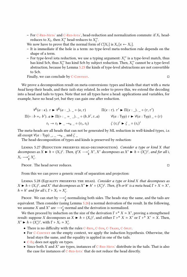
– For C-Red-Meta’ and C-Red-Iota’, head-reduction and normalization commute: if X1 head-
reduces to X2, then X ′′1head-reduces to X ′′
2.
We now have to prove that the normal form of C[Xi ] is Xc [x ← Xi ].
– It is immediate if the hole is a term: no type-level meta-reduction rule depends on the
shape of a term.
– For type-level iota reduction, we use a typing argument: X ′′1is a type-level match, thus
has kind Sch, thus X ′′2has kind Sch by subject reduction. Then, X ′′
2cannot be a type-level
abstraction, because by Lemma 5.23 the kinds of type-level abstractions are not convertible
to Sch.Finally, we can conclude by C-Context. □
We prove a decomposition result on meta-conversions: types and kinds that start with a meta
head keep their heads, and their tails stay related. In order to prove this, we extend the decoding
into a head and tails to types. Note that not all types have a head: applications and variables, for
example, have no head yet, but they can gain one after reduction.
∀♯ (α : κ). τ � ∀♯ (α : _). _ ◦ (κ,τ ) Π(x : τ ). τ ′ � Π(x : _). _ ◦ (τ ,τ ′)
Π(⋄ : b =τ b′). a � Π(⋄ : _ =_ _). _ ◦ (b,b
′,τ ,a) ∀(α : Typ) τ � ∀(α : Typ) _ ◦ (τ )
τ1 → τ2 � _→tt _ ◦ (τ1,τ2) ζ (τi )i � ζ _ ◦ (τi )
i
The meta-heads are all heads that can not be generated by ML reduction in well-kinded types, i.e.
all except ∀(α : Typ) _, _→tt _ and ζ _The head-decomposition of types and kinds is preserved by reduction:
Lemma 5.27 (Reduction preserves head-decomposition). Consider a type or kind X that
decomposes as X � h ◦ (Xi )i. Then, if X −→∗
♯X ′, X ′ decomposes as X ′ � h ◦ (X ′i )
i, and for all i ,
Xi −→∗
♯X ′i .
Proof. The head never reduces. □
From this we can prove a generic result of separation and projection:
Lemma 5.28 (Eqality preserves the head). Consider a type or kind X that decomposes as
X � h ◦ (Xi )i, andX ′ that decomposes asX ′ � h′ ◦ (X ′j )
j. Then, ifh orh′ is a meta head, Γ ⊢ X ≃ X ′,
h = h′ and for all i , Γ ⊢ Xi ≃ X ′i .
Proof. We can start by −→t♯-normalizing both sides. The heads stay the same, and the tails are
equivalent. Then consider (using Lemma 5.26) a normal derivation of the result. In the following,
we assume X and X ′ are −→t♯-normal and the derivation is normalized.
We then proceed by induction on the size of the derivation Γ ⊢n X ≃ X ′, proving a strengthened
result: suppose X decomposes as X � h ◦ (Xi )i, and either Γ ⊢n X ≃ X ′ or Γ ⊢n X ′ ≃ X . Then,
X ′ � h ◦ (X ′i )i, with Γ ⊢ Xi ≃ X ′i .
• There is no difficulty with the rules C-Refl, C-Sym, C-Trans, C-Split.
• For C-Context on the empty context, we apply the induction hypothesis. Otherwise, the
head stays the same, and the equality is applied in one of the tails.
• C-Eq does not apply on types.
• Since both X and X ′ are types, instances of C-Red-Meta’ distribute in the tails. That is also
the case for instances of C-Red-Iota’ that do not reduce the head directly.

• For −→hι : X has a head, so the reduction is necessarily X ′ −→h
ι X . X and X ′ cannot bekinds, so they are types τ and τ ′. We have τ ′ = match dj (ui )
i with (dj (xi j )i → τj )
j ∈Jand
τ = τj [xi j ← ui ]i. The term τj has the same head as τ . Moreover, inverting the last syntactic
rule of a kinding derivation for τ ′, we obtain Γ ⊢ τj : Sch. We want to show that this is
impossible. Consider the last syntactic rule of this derivation. It is of the form Γ ⊢ τj : κ, withκ , Sch. Moreover, we have Γ ⊢ κ ≃ Sch. But this is absurd by Lemma 5.23. □
Then, we get subject reduction for term-level part of −→♯ . We first prove an inversion lemma:
Lemma 5.29 (Inversion, meta, term level). Consider an environment Γ.
• If Γ ⊢ λ♯ (x : τ ′1). a : Π(x : τ1). τ2, then Γ,x : τ1 ⊢ a : τ2.
• If Γ ⊢ Λ♯ (α : κ ′). a : ∀♯ (α : κ). τ , then Γ,α : κ ⊢ a : τ .• If Γ ⊢ λ♯ (⋄ : b ′
1=τ ′ b
′2). a : Π(⋄ : b1 =τ b2). τ
′′, then Γ, (b1 =τ b2) ⊢ a : τ ′′.
Proof. Similar to the proof of Lemma 5.24. □
Lemma 5.30 (Subject reduction for −→♯). Let Γ be a well-formed context. Suppose X −→♯ X′.
Then, if Γ ⊢ X : Y , Γ ⊢ X ′ : Y .
Proof. Add the term-level part to the proof of Lemma 5.25 □
We can normalize further the conversions between two −→♯ normal forms:
Lemma 5.31 (Normal derivations, type-level meta-reduction). Suppose Γ ⊢ X1 ≃ X2, where
X1 and X2 are normal terms, types or kinds for −→♯ . Then, there exists a derivation of Γ ⊢n X1 ≃ X2,
where Γ ⊢n X1 ≃ X2 is a limited version of Γ ⊢ X1 ≃ X2 where the rule C-Red-Meta is limited to −→a♯.
More precisely, this judgment is defined from the following rules:
C-Refl
Γ ⊢ X : Y
Γ ⊢n X ≃ X
C-Sym
Γ ⊢n X1 ≃ X2
Γ ⊢n X2 ≃ X1
C-Trans
Γ ⊢n X1 ≃ X2 Γ ⊢n X2 ≃ X3
Γ ⊢n X1 ≃ X3
C-Red-Iota’
X1 −→ι X2 Γ ⊢ X1 : Y1 Γ ⊢ X2 : Y2
Γ ⊢n X1 ≃ X2
C-Red-Meta’
X1 −→a♯X2 Γ ⊢ X1 : Y1 Γ ⊢ X2 : Y2
Γ ⊢n X1 ≃ X2
C-Context
Γ ⊢ C[Γ′ ⊢ X1 : Y ′] : Y Γ ⊢n X1 ≃ X2
Γ ⊢n C[X1] ≃ C[X2]
C-Eq
a1 −→∗
♯u1 a2 −→
∗
♯u2 (a1 =τ a2) ∈ Γ
Γ ⊢n u1 ≃ u2
C-Split
(di : ∀(αk )k (τi j )j → ζ (αk )k )i(Γ, (xi j : τi j [(αk ← τk )k ])j , (u = di (xi j )) ⊢
n X1 ≃ X2)i Γ ⊢ u : ζ (τk )k
Γ ⊢n X1 ≃ X2
Proof. Similar to Lemma 5.26. □
We can now prove a projection result for eML. The corresponding separation result is more
complex and will be proved separately.
Lemma 5.32 (Projection for eML). Consider X and X ′ decomposing as X � h ◦ (Xi )iand
X ′ � h ◦ (X ′i )i. Suppose Γ ⊢ X ≃ X ′. Then, Γ ⊢ Xi ≃ X ′i .

Proof. The result for non-ML heads is already implied by the previous lemma. We can suppose
that X and X ′ are types τ and τ ′ and are normal for −→♯ , and that we have a normal derivation of
Γ ⊢ τ ≃ τ ′.We derive a stronger result: we define a function tails(h;τ ) that returns the tails of a type,
assuming it has a given eML head. We use Anya to stand for any well-typed term, Anyt for awell-kinded type, and Anyk for a well-sorted kind (for example, Anya = λ (x : Anyt). x , Anyt =∀(α : Typ) α and Anyk = Typ).
tails(h;τ ) = (Xi )i
if τ � h ◦ (Xi )i
tails(h;match a with (Pi → τi )i ) = (match a with (Pi → Xi j )
i ) j if tails(h;τi ) = (Xi j )j
tails(h;τ ) = (Any)i
Note that the action of taking the tail commutes with substitution of terms: tails(h;τ [x ← u]) =tails(h;τ )[x ← u]. Moreover, if τ is well-typed, its tails tails(h;τ ) are well-typed or kinded (by
inversion of the last syntax-directed rule of a kinding of τ ).Then, we show by induction on a normal derivation that whenever Γ ⊢ τ ≃ τ ′, for any ML head
h, Γ ⊢ tails(h;τ )i ≃ tails(h;τ ′)i . This is sufficient, because tails(h;τ )i = Xi and tails(h;τ ′)i = X ′i .We suppose that the reductions are head-reductions, and that all applications of C-Context use
only a shallow context.
• For C-Refl, invert the typing derivation to ensure that the tails are well-typed.
• There is no difficulty for C-Sym and C-Trans.
• For C-Split: prove the equality in each branch and merge using C-Split.
• The rule C-Eq does not apply in a typing context.
• For C-Red-Iota’, the only possible head-reduction is a reduction of a type-level match: suppose
we have τ = match dj (ui )i with (dk (xki )
i → τk )kand τ ′ = τj [x ji ← ui ]
i. Then, compute
the tail: tails(h;τ )l = match dj (ui )i with (dk (xki )
i → Xkl )kwhere Xkl = tails(h;τk )l and
tails(h;τ ′) = tails(h;τj )[x ji ← ui ]i. The tails are well-typed, and reduce to one another, thus
we can conclude by C-Red-Iota’
• For C-Context, consider the different cases:
– If the context is of the form C = match C ′ with (Pi → τi )iand is applied to X1 and X2, we
have Γ ⊢ C ′[X1] = C ′[X2] ≃. Then we can substitute in the tails.
– If the context is of the form C = match a with (Pi → τi )i | Pj → C ′, we can use the
induction hypothesis: the tails of the case where the hole is are equal, so we can substitute
in the global tails.
– All other contexts distribute immediately in the tails. □
We obtain subject reduction.
Theorem 5.33 (Subject reduction). Suppose Γ is well-formed, X −→ X ′ and Γ ⊢ X : Y . Then,Γ ⊢ X ′ : Y .
Proof. We need to prove subject reduction for −→ι and −→β . We prove this for head-reduction
as in the other subject reduction results (see Lemma 5.25). For −→ι , we can use the same technique
as in the other proofs since C-Red-Iota’ allows injecting −→ι in the equality.
For −→β , there are two cases. If we reduce an application, the evaluation context E is not
dependent according to Lemma 5.21. In the other cases, the reduction is actually a−→ι reduction. □
Theorem 5.34 (Eqal things have the same types, kinds, and sorts). Consider a context Γ.Suppose Γ ⊢ X1 ≃ X2. Then, for all Y , Γ ⊢ X1 : Y if and only if Γ ⊢ X2 : Y .
Proof. By induction on a derivation. This is immediate for reflexivity, transitivity and symmetry.
Reduction preserves types by subject reduction. Substitution preserves types too. □

Dt ::= [] ♯ a | [] ♯ τ | [] ♯ ⋄
Dv ::= [] ♯ a | [] ♯ τ | [] ♯ ⋄ | [] a | [] τ | match [] with P → a
ct ::= λ♯ (x : τ ). τ | Λ♯ (α : κ). τ | λ♯ (⋄ : a =τ a). τ
cv ::= λ♯ (x : τ ). a | λ♯ (x : τ ). a | Λ♯ (α : κ). a | λ♯ (⋄ : a =τ a). a
| λ (x : τ ). a | fix (x : τ ) x . a | Λ (α : Typ). a | d (a)
Fig. 17. Destructors and constructors
We can now use the simplified version of equality (C-Eq, C-Red-Iota, C-Red-Meta).
5.5 Soundness for −→♯
We now show that meta-reductions are sound in any environment, and ML reductions are sound in
the empty environment.
We define (see Figure 17) constructors ct and cv at the level of types and terms, and destructor
contexts, or simply destructors, Dt and Dv for types and terms. Some destructors destruct terms
but return types.
Moreover, we defined the predicate meta on constructors and destructors that do not belong to
eML (hence, use a meta-construction at the toplevel)
Theorem 5.35 (Soundness, meta). Let Γ be an environment. Then:
• If Γ ⊢ Dt[ct] : Y , then Dt[ct] −→h.
• If Γ ⊢ Dv[cv] : Y , then Dv[cv] −→h.
Proof. By case analysis on the destructor. We consider the case Dt = [] ♯ τ . Consider the variouscases for ct: by Lemma 5.28, the only possible case is ct = Λ♯ (α : κ). τ ′. Then, Dt[ct] reduces. □
5.6 Reducing mML to eML
We will now show that any mML term that can be typed in an environment without any meta
construct normalizes by −→♯ to an eML term of the same type. It does not suffice to normalize
the term and check that it does not contain any mML syntactic construct and conclude by subject
reduction: we have to show the existence of an eML typing derivation of the term.
Definition 5.36 (Meta-free context). A meta-free context is a context where the types of all (term)
variables have kind Sch, and all type variables have kind Typ. A term is said to be meta-closed if it
admits a typing under a meta-free context. A term is said to be eML-typed if moreover its type has
kind Sch. A type is said to be eML-kinded if moreover it has kind Sch (or one of its subkinds).
Theorem 5.37 (Classification of meta-normal forms). Consider a normal, meta-closed term
or type. Then, it is an eML term or type, or it is not eML-typed (or eML-kinded) and starts with a meta
abstraction.
Proof. By induction on the typing or kinding derivation. Consider the last rule of a derivation:
• If it is a kind conversion K-Conv, by Lemma 5.23, it is a trivial conversion.
• If it is a type conversion, by Theorem 5.34, the kind of the type is preserved.
• If it is a construct in ML syntax: the subderivations on terms and types are also in meta-closed
environments and eML-typed or eML-kinded, and we apply the induction hypothesis.
• If it is a meta-abstraction, it is not eML-typed or eML-kinded because of non-confusion of
kinds.

• If it is a meta-application: let us consider the case of term-level meta type-application. The
other cases are similar. We have a = b ♯ τ . b is typeable in a meta-closed context but is not
eML-typed. Thus, it is a meta-abstraction. By soundness, a reduces, thus is not a normal
form. □
We prove that allmML derivations on eML syntax that can be derived inmML can also be derived
in eML. The difficulty comes from equalities: transitivity allows us to make mML terms appear in
the derivation; these must be reduced to eML while maintaining a valid typing derivation.
Theorem 5.38 (eML terms type in eML). In eML, consider an environment Γ; terms (resp. types,
kinds) X , X1, and X2; and a type (resp. kind, sort) Y . Then:
• If ⊢ Γ in mML, then there is a derivation of ⊢ Γ in eML.• If Γ ⊢ X : Y in mML, then there is a derivation of Γ ⊢ X : Y in eML.• If Γ ⊢ X1 ≃ X2 in mML, then there is a derivation of Γ ⊢ X1 ≃ X2 in eML.
Proof. By mutual induction.
We need to strengthen the induction for the typing derivations: we prove that, for any mMLtype, kind or sort Y ′, if Γ ⊢ X : Y ′, Y ′ reduces to Y in eML and Γ ⊢ X : Y . Then notice that the
conversions only happen between normal eML terms, so we can apply the results on equalities.
For equalities, normalize the derivations as in Lemma 5.31, but simultaneously transform the
typing derivations into eML derivations (this must be done simultaneously otherwise we cannot
control the size of the new derivations). □
The main result of this section follows.
Theorem 5.39 (Reduction from mML to eML). If Γ ⊢ a : τ and Γ ⊢ τ : Sch are eML judgments
that are derivable in mML, then there exists a reduction a −→♯ a′such that Γ ⊢ a′ : τ holds in eML.
Note that this implies that eML also admits subject reduction.
Proof. The well-typed term a normalizes by −→♯ to an irreducible term a′. By subject reduction,Γ ⊢ a′ : τ . By classification of values, it is an eML term. By Theorem 5.38, there is a derivation of
Γ ⊢ a′ : τ in eML. □
5.7 Soundness, via a Logical Relation for −→ι
We prove that −→ι is normalizing, on all terms (including ill-typed terms):
Lemma 5.40 (Nomalization for −→ι ). The reduction −→ι is strongly normalizing.
Proof. We say that a term, type or kind is good if it admits no infinite reduction sequence, and if
it reduces to Λ (α : Typ). u, for all good types τ , u[α ← τ ] is good. Goodness is stable by reduction.
We will prove the following property by induction on a term, type or kindX : supposeγ associates
type and term variables to good terms and types. Then, γ (X ) is good. Let us consider the differentcases:
• If X is a variable, γ (X ) is good by hypothesis.
• If X = Λ (α : Typ). u: by induction hypothesis, γ (u) is good for all γ , thus γ (X ) admits no
infinite reduction sequence. Moreover, if X reduces to Λ (α : Typ). u ′, u ′[α ← τ ] can be
obtained by reduction from (γ [α ← τ ]) (u), and thus is good.
• Suppose no head-reduction occurs from γ (X ). Then, since the subterms normalize, γ (X )normalizes. We will now only consider the terms where head-reduction could occur.
• If X = a τ , suppose γ (X ) reduces to a term that head-reduces. Then, this term is X ′ = (Λ (α :
Typ). u) τ , that reduces to u[α ← τ ]. Since a is good, the result is good too.

• If X = let x = a1 in a2 has a head-reduction, it is from let x = u in a′2to a′
2[x ← u], where
γ (a1) reduces to u and γ (a2) reduces to a′2. The term u is good, thus (γ [x ← u])a2 is good
and reduces to a′2[x ← u].
• Similarly for type and term-level pattern matching.
□
We then prove soundness of the −→ι reduction. This is done via a logical relation (essentially,
implementing an evaluator for the non-expansive terms of eML with the reduction −→ι ). This then
allows proving (syntactically) that all conversions in the empty environment are between types
having the same head (up to reduction). Let us note u −→!
ι v if all reduction paths from u terminate
at v .We start by defining a unary logical relation specialized to −→ι in Figure 18. It includes an
interpretation V[τ ]γ of values of type τ , an interpretation E[τ ]γ of terms as normalizing to the
appropriate values, an interpretation G[γ ]τ of the typing environments as environments associ-
ating variables to non-expansive terms. We also define binary interpretations (although they are
interpreted in an unary environment). EqE[τ ]γ of equality at type τ , via an interpretation EqV[τ ]γof equality for values. We will omit the typing and equality conditions in the definitions. The unary
interpretation only contains terms that normalize, while the binary interpretation contains both
pairs of terms that normalize by −→ι , and pairs of terms stuck on a beta-reduction step. We write
⊢ γ : Γ to mean that γ is a well-typed environment that models Γ, and ⊢ γ1 ≃ γ2 if all components
of γ1 and γ2 are equal.
The definition of the interpretations is well-founded, by induction on types, and, for datatypes, by
induction on the values (because the values appearing inside datatype constructors are necessarily
values of a datatype, or functions from terms).
Definition 5.41 (Valid environment). An environment γ is valid if for all α such that γ (α ) =(τ , S,R),
• For all u ∈ S , ∅ ⊢ u : τ .• The restriction of R to S is an equivalence relation.
Lemma 5.42 (Definition of the interpretations). The interpretations are defined for wall-
kinded terms and well-formed environments:
• If ⊢ Γ, G[Γ] is well-defined and all its elements are valid, and EqG[Γ] is well-defined and
reflexive on G[Γ].
• If Γ ⊢ τ : Sch, for all γ ∈ G[Γ], E[τ ]γ is defined, all its elements are non-expansive terms of
type γ (τ ), and EqE[τ ]γ is an equivalence relation on E[τ ]γ .
Proof. By mutual induction on the kinding and well-formed derivations. □
As usual, we need to prove a substitution result:
Lemma 5.43 (Substitution). Consider a valid environment γ . Then,
• E[τ [x ← u]]γ = E[τ ]γ [x←u]
• EqE[τ [x ← u]]γ = EqE[τ ]γ [x←u]
• E[τ [α ← τ ′]]γ = E[τ ]γ [α←(γ (τ ′),E[τ ′]γ ,EqE[τ ′]γ )]• EqE[τ [x ← τ ′]]γ = EqE[τ ]γ [α←(γ (τ ′),E[τ ′]γ ,EqE[τ ′]γ )]
Proof. By induction on τ . □
We also need to prove that reducing a value in the environment does not change the interpretation:

G[Γ] ⊆ {γ | ⊢ γ : Γ}G[Γ,x : τ ] = {γ [x ← u] | γ ∈ G[Γ] ∧ u ∈ E[τ ]γ }
G[Γ,α : Typ] = {γ [α ← (γ (τ ),E[τ ]γ ,EqE[τ ]γ )] | γ ∈ G[Γ]}
G[Γ, (a1 =τ a2)] = {γ ∈ G[Γ] | a1,a2 non-expansive =⇒ (γ (a1),γ (a2)) ∈ EqE[τ ]γ }
E[τ ]γ ⊆ {a | ∅ ⊢ a : γ (τ )}E[τ ]γ = {u | ∃ (v ) u −→!
ι v ∧v ∈ V[τ ]γ }
V[τ ]γ ⊆ {v | ∅ ⊢ v : γ (τ )}V[α]γ = γ (α )V[τ1 → τ2]γ = {fix (x : τ ′
1→ τ ′
2) y. a}
V[∀(α : Typ) τ ]γ = {(Λ (α : Typ). v ) | ∀ (∅ ⊢ τ ′ : Typ) v[α ← τ ′] ∈ E[τ ]γ [α←(τ ′,E[τ ′]γ ,EqE[τ ′]γ )]}
V[ζ (τi )i]γ = {(d (vj )
j ) | (d : ∀(αi : Typ)i (τj ) j → ζ (αi )i ) ∧ ∀ (j ) vj ∈ Vk [τj [αi ← τi ]
i]γ }
V[match a with (di (xi j )j → τi )
i]γ =
{V[τj ]γ [xi j←vj ]j if γ (a) −→!
ι di (vj )j
∅ otherwise
EqG[Γ] ⊆ {(γ1,γ2) | ⊢ γ1 ≃ γ2}
EqG[Γ,x : τ ] = {(γ1[x ← u1],γ2[x ← u2]) | (γ1,γ2) ∈ EqG[Γ] ∧ (u1,u2) ∈ EqE[τ ]γ1}
EqG[Γ,α : Typ] =
(γ [α ← (γ1 (τ1),E[τ1]γ1
,EqE[τ2]γ1)],
γ [α ← (γ2 (τ2),E[τ1]γ2,EqE[τ2]γ2
)]
) �������
(γ1,γ2) ∈ EqG[Γ]
∧ E[τ1]γ1= E[τ2]γ2
∧ EqE[τ1]γ1= EqE[τ2]γ2
EqG[Γ, (a1 =τ a2)] =
{(γ1,γ2) ∈ G[Γ]
�����a1,a2 non-expansive =⇒
(γ1 (a1),γ1 (a2)) ∈ EqE[τ ]γ1∧ (γ2 (a1),γ2 (a2)) ∈ EqE[τ ]γ2
}EqE[τ ]γ ⊆ {(a1,a2) | ∅ ⊢ a1 ≃ a2}
EqE[τ ]γ =
{(u1,u2)
�����(∃ (v1 v2) u1 −→
!
ι v1 ∧ u2 −→!
ι v2 ∧ (v1,v2) ∈ EqV[τ ]γ )∨ (∀ (v1 v2) ¬(u1 −→
!
ι v1) ∧ ¬(u2 −→!
ι v2))
}EqV[τ ]γ ⊆ {(v1,v2) | ∅ ⊢ v1 ≃ v2}
EqV[α]γ = γ (α )EqV[τ → τ ′]γ = {(fix (x : τ1 → τ ′
1) y. a1, fix (x : τ2 → τ ′
2) y. a2)}
EqV[∀(α : Typ) τ ]γ =
{(Λ (α : Typ). v1,Λ (α : Typ). v2
) �����∀ (∅ ⊢ τ ′ : Typ)
(v1[α ← τ ′],v2[α ← τ ′]) ∈ V[τ ]γ [α←EqE[τ ′]γ ]
}EqV[ζ (τi )
i]γ =
{(d (vj )
j ,d (w j )j )�����d : ∀(αi : Typ)i (τj ) j → ζ (αi )
i
∧((vj ,w j ) ∈ EqV[τj [αi ← τi ]i]γ )
j
}EqV[match a with (di (xi j )
j → τi )i]γ =
{EqV[τj ]γ [xi j←vj ]j if γ (a) −→!
ι di (vj )j
∅ otherwise
Fig. 18. Logical relation for −→ι
Lemma 5.44 (Reduction in the environment). Consider a valid environment γ , and u −→ι u′.
Then,
• E[τ ]γ [x←u] = E[τ ]γ [x←u′]• EqE[τ ]γ [x←u] = EqE[τ ]γ [x←u′]
Proof. By induction on τ . The term variables in γ are used for substituting into types for the
typing side-conditions. Since ∅ ⊢ u ≃ u ′, the typing side-conditions stay true by Lemma 5.16.
They also occur in the interpretation of pattern matching. But, for all terms a, (γ [x ← u]) (a) and(γ [x ← u ′]) (a) normalize to the same term. □
Lemma 5.45 (Eqality in the environment). Consider a valid environment γ and τ1, S,R such
that γ [α ← (τ1, S,R)] is valid. Suppose ∅ ⊢ τ1 ≃ τ2. Then,
• γ [α ← (τ2, S,R)] is valid;• for all types τ , E[τ ]γ [α←(τ1,S,R )] = E[τ ]γ [α←(τ2,S,R )];
• for all types τ , EqE[τ ]γ [α←(τ1,S,R )] = EqE[τ ]γ [α←(τ2,S,R )].
Proof. By induction. The type τ1 occurs only in the conclusion of typing derivations. Use
conversion and ∅ ⊢ τ1 ≃ τ2 to get the same derivations with τ2. □
Lemma 5.46 (Reduction preserves interpretation). Suppose τ −→ι τ′. Then,
• E[τ ]γ = E[τ ′]γ ;• EqE[τ ]γ = EqE[τ ′]γ .
Proof. Wewill show the lemma for E[τ ]γ . We eliminate the context of the reduction by induction.
If we pass to a reduction between terms, it is in the argument of a type-level match. Then, the two
terms normalize to the same term. The only type-level reduction is the reduction of the type-level
match:
match dj τj (ui )i with (dj τj (x ji )
i → τj )j ∈J −→h
ι τj [x ji ← ui ]i
Let us show that the two types have the same interpretation. We have dj τj (ui )i −→!
ι dj τj (vi )i,
where ui −→!
ι vi . Thus, the interpretation of the left-hand side is E[τ ]γ [x ji←vi ]i = E[τ ]γ [x ji←ui ]i
by Lemma 5.44. By substitution (Lemma 5.43), E[τ ]γ [x ji←ui ]i = E[τ [x ji ← ui ]i]γ . This is the
interpretation of the right-hand side. □
Lemma 5.47 (Evaluation for −→ι ). Suppose ⊢ Γ. Then:
• if Γ ⊢ u : τ , then for all γ ∈ G[Γ], γ (u) ∈ E[τ ]γ ;
• if Γ ⊢ τ1 ≃ τ2, then for all (γ1,γ2) ∈ EqG[Γ], E[τ1]γ = E[τ2]γ and EqE[τ1]γ1= EqE[τ2]γ2
;
• if Γ ⊢ a1 ≃ a2 and Γ ⊢ a1 : τ , then for all (γ1,γ2) ∈ EqG[Γ], (γ1 (a1),γ2 (a2)) ∈ EqE[τ ]γ1;
• if Γ ⊢ τ : Sch, then for all (γ1,γ2) ∈ EqG[Γ], EqE[τ ]γ1= EqE[τ ]γ2
;
• if Γ ⊢ a : τ , then for all (γ1,γ2) ∈ EqG[Γ], (γ1 (a),γ2 (a)) ∈ EqE[τ ]γ1.
Proof. We prove these results by mutual induction on the derivations.
For the result on typing derivations, let us consider the different rules:
• For Var on x : τ : by hypothesis, γ (x ) ∈ E[τ ]γ .
• For Conv: use the second lemma to show the interpretations of the two types are the same.
• For Fix: any two well-typed abstractions are linked at an arrow type.
• The rule App cannot occur as the first rule in the typing of a non-expansive term.
• For TAbs:
TAbs
Γ,α : Typ ⊢ u : τ
Γ ⊢ Λ (α : Typ). u : ∀(α : Typ) τ
Consider γ ∈ G[Γ] and ∅ ⊢ τ ′ : Typ. Λ (α : Typ). u normalizes to Λ (α : Typ). v with u −→!
ι v .By induction hypothesis, (γ [α ← τ ′]) (u) ∈ E[τ ]γ [α←(τ ′,E[τ ′]γ ,EqE[τ ′]γ )]. Moreover, it reduces
to (γ [α ← τ ′]) (v ) = γ (v )[α ← τ ′]. Thus, γ (v )[α ← τ ′] ∈ E[τ ]γ [α←(τ ′,E[τ ′]γ ,EqE[τ ′]γ )].
• For TApp:
TApp
Γ ⊢ τ ′ : Typ Γ ⊢ u : ∀(α : Typ) τ
Γ ⊢ u τ ′ : τ [α ← τ ′]
Consider γ ∈ G[Γ]. There exists τ ′′ such that γ (τ ′) −→!
ι τ′′. Then, ∅ ⊢ τ ′′ : Typ. There exists
v such that γ (u) −→!
ι v . By inductive hypothesis, v ∈ V[∀(α : Typ) τ ]γ . Thus, there exists

v ′ such that v = Λ (α : Typ). v ′, and v ′[α ← τ ′′] ∈ E[τ ]γ [α←(τ ′′,E[τ ′′]γ ,EqE[τ ′′]γ )] = E[τ [α ←τ ′′]]γ = E[τ [α ← τ ′]]γ by Lemmas 5.43 and 5.46. We need to prove γ (u τ ′) ∈ E[τ [α ← τ ′]]γ .But we have γ (u τ ′) −→∗ι (Λ (α : Typ). v ′) τ ′′ −→ι v
′[α ← τ ′′].
• The other cases are similar.
For the result on equalities between types, by induction on a derivation. We suppose that the
context rule is always used with a shallow context.
• For C-Sym and C-Trans, use the induction hypothesis and symmetry/transitivity of equality.
• For C-Refl, use reflexivity on types.
• For C-Context: apply the induction hypothesis on the modified subterm if it is a type, and
reflexivity on the other subterms.
• Otherwise, it is the argument of a type-level pattern matching. We have Γ ⊢ a1 : ζ (τi )i,
Γ ⊢ a2 : ζ (τi )i, and Γ ⊢ a1 ≃ a2. By the third result, (γ1 (a1),γ2 (a2)) ∈ EqE[ζ (τi )
i]γ1
. If
both do not normalize to a value, the two interpretations of the pattern matching are empty.
Otherwise they normalize to d (v1j )jand d (v2j )
jsuch that (v1j ,v2j ) ∈ EqE[τj ]γ1
where the τjare the types of the arguments. Thus, (γ1[x j ← v1j ]
j ,γ2[x j ← v2j ]j ) ∈ EqG[Γ, (x j : τj )
j], and
we can interpret the selected branch in these environments.
• For C-Split on a term Γ ⊢ u : τ ′, use reflexivity on types to prove that (γ1 (u),γ2 (u)) ∈EqE[τ ′]γ1
. Moreover, γ1 (u) ∈ E[τ ′]γ1, thus the terms normalize to a value. Then, select the
case corresponding to the constructor, construct an environment as in the previous case, and
use the induction hypothesis.
• For C-Red-Iota, suppose we have a head-reduction (otherwise, use C-Context). Then, it is
the reduction of a pattern matching. Proceed as in C-Split.
• The rule C-Eq does not apply on types.
For the result on equalities between terms:
• The cases of C-Sym, C-Trans and C-Split are similar to the same cases on types.
• For C-Refl, use reflexivity on terms.
• For C-Red-Iota, proceed as in C-Red-Iota for types.
• For C-Eq, consider the two equal terms u1,u2. From γ1 we get (γ1 (u1),γ1 (u2)) ∈ EqE[τ ]γ1.
Moreover, by reflexivity on u2, (γ1 (u2),γ2 (u2)) ∈ EqE[τ ]γ1. We conclude by transitivity of
EqE[τ ]γ1.
• For C-Context, examine the different typing rules as in the first result, and use reflexivity
when needed.
For the reflexivity results, examine the different typing rules as in the first result. Take special care
for variables. The interpretations of the type variables are the same. For term variables appearing in
terms, they are bound to related terms. Finally, for type-level pattern matching, the interpretations
of the term in the environments are related by reflexivity. □
The following result is then a direct consequence:
Lemma 5.48 (Separation for −→ι ). Suppose ∅ ⊢ τ1 ≃ τ2. Then if τ1 and τ2 have a head, it is the
same.
Proof. Apply the previous result with the empty environment. The interpretations of types
with distinct heads are distinct. □
Theorem 5.49 (Soundness, empty environment).
• If ∅ ⊢ Dt[ct] : Y , then Dt[ct] −→h.
• If ∅ ⊢ Dv[cv] : Y , then Dv[cv] −→h.
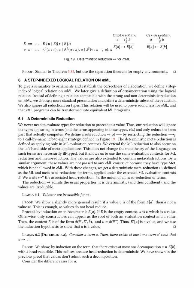
E ::= . . . | E ♯u | E ♯ τ | E ♯ ⋄
v ::= . . . | λ♯ (x : τ ). a | Λ♯ (α : κ). a | λ♯ (⋄ : a =τ a). a
Ctx-Det-Meta
a −→h♯b
E[a] 7→ E[b]
Ctx-Beta-Meta
a −→hβ b
E[a] 7→ E[b]
Fig. 19. Deterministic reduction 7→ for mML
Proof. Similar to Theorem 5.35, but use the separation theorem for empty environments. □
6 A STEP-INDEXED LOGICAL RELATION ON mML
To give a semantics to ornaments and establish the correctness of elaboration, we define a step-
indexed logical relation on mML. We later give a definition of ornamentation using the logical
relation. Instead of defining a relation compatible with the strong and non-deterministic reduction
onmML, we choose a more standard presentation and define a deterministic subset of the reduction.
We also ignore all reductions on types. This relation will be used to prove soundness for eML, andthat eML programs can be transformed into equivalent ML programs.
6.1 A Deterministic Reduction
We never need to evaluate types for reduction to proceed to a value. Thus, our reduction will ignore
the types appearing in terms (and the terms appearing in these types, etc.) and only reduce the term
part that actually computes. We define a subreduction 7→ of −→ by restricting the reduction −→♯
to a call-by-name left-to-right strategy, defined in Figure 19. The deterministic meta-reduction is
defined as applying only in ML evaluation contexts. We extend the ML reduction to also occur on
the left-hand side of meta-applications. This does not change the metatheory of the language, as
such terms are necessarily ill-typed, but it allows us to use the same evaluation contexts for ML
reduction and meta-reduction. The values are also extended to contain meta-abstractions. By a
similar argument, these values are not passed to any eML construct because they have typeMet,which is not allowed in eML. With these changes, we get a deterministic meta-reduction 7→ defined
as the ML and meta head-reductions for terms, applied under the extended ML evaluation contexts
E. We write 7→hthe associated head-reduction, i.e. the union of all head-reduction of terms.
The reduction 7→ admits the usual properties: it is deterministic (and thus confluent), and the
values are irreducible.
Lemma 6.1. Values v are irreducible for 7→.
Proof. We show a slightly more general result: if a value v is of the form E[a], then a not a
value v ′. This is enough, as values do not head-reduce.
Proceed by induction on v . Assume v is E[a]. If E is the empty context, a is v which is a value.
Otherwise, only constructors can appear as the root of both an evaluation context and a value.
Then, the context E is of the form d (v ′,E ′,b), and v = d (v ′′). Thus, E ′[a] is a value, and we use
the induction hypothesis to show that a is a value. □
Lemma 6.2 (Determinism). Consider a term a. Then, there exists at most one term a′ such that
a 7→ a′.
Proof. We show, by induction on the term, that there exists at most one decomposition a = E[b],
with b head-reducible. This suffices because head-reduction is deterministic. We have shown in the
previous proof that values don’t admit such a decomposition.
Consider the different cases for a.

• a is an abstraction or a fixed point: it does not decompose further since there is no appropriate
non-empty evaluation context.
• a is d (a)ii : either it is a value, or we can decompose the sequence (a)ii = (b) jj ,b, (v )kk , with b
not a value. Necessarily, E = d ((b) jj ,E′, (v )kk ) (because E cannot be empty: constructors do
not reduce). But then, b admits a unique decomposition as E ′[b ′].• a is let x = a1 in a2: If a1 is a value, then it does not decompose, and the only possible context
is the empty context []. Otherwise, it admits at most one decomposition E ′[b], and a admits
only the decomposition let x = E ′[b] in a2.
• a is a1 a2: If a2 is not a value, a does not head-reduce and the only possible decomposition of
E is a1 E ′. Since a2 decomposes uniquely, E ′ is unique, thus E is unique. Otherwise a2 is a
value v , If a1 is not a lambda, a does not head-reduce, and the only possible decomposition of
E is E ′ v . By induction, E ′ is unique. If both are values, the only possible evaluation context
is the empty context.
• Cases for all others applications are similar, except that there is no context allowing the
reduction of the right-hand side of the application, thus it is not necessary to check whether
it is a value.
□
We can now link the deterministic reduction 7→ and the full reduction −→.
We first note that ML reduction is impossible on values:
Lemma 6.3. If v −→ a, then we actually have v −→♯ a and a is a value.
Proof. The ML reduction −→β is included in 7→, and values do not reduce for 7→. By induction
on the values, we can prove that redexes only occur under abstractions. Thus, the term remains a
value after reduction. □
We write −→λ the reduction that only reduces ML term abstractions. It is also the subset of −→βreductions that are not included in −→ι .
Lemma 6.4 (Commutations for well-typed terms). Meta-reductions can always be done first,
moreover, β-reductions and ι-reductions commute. More precisely, assume X1 is a well-typed term:
• If X1 −→ι X2 −→♯ X3, then X1 −→♯ X4 −→∗ι X3 for some X4.
• If X1 −→λ X2 −→♯ X3, then X1 −→∗
♯X4 −→λ X3 for some X4.
• If X1 −→λ X2 and X1 −→ι X3, then X2 −→∗ι X4 and X3 −→λ X4 for some X4.
Proof. For the first two commutations: a typing argument prevents −→ι and −→λ from creating
meta-redexes. For the third property: note that −→ι cannot duplicate a −→λ redex in an evaluation
context. □
Lemma 6.5 (Normalization for −→ι and −→♯). The union of −→ι and −→♯ is strongly normal-
izing on well-typed terms.
Proof. Consider a term X . By König’s lemma (since by Theorem 5.2, there is a finite number of
possible reductions from one term), all possible −→♯ reduction sequences from X are of length at
most k for some k . Consider an infinite (−→ι ∪ −→♯ ) reduction sequence from X . It has k −→♯
reductions or less. Otherwise, we could use Lemma 6.4 to put k + 1 −→♯ reductions at the start of
the sequence. Thus, after the last −→♯ reduction, there is an infinite sequence of −→ι reduction.
But this is impossible by Lemma 5.40. □
Lemma 6.6 (Weak normalization implies strong normalization). Consider a term a. Supposethere exists a terminating reduction path from a. Then, all reduction sequences are finite.

Proof. We show that all reduction sequences from a have the same number of −→λ reductions.
We can, without loss of generality (by Lemma 6.4) assume that a is meta-normal and that the
reduction path is meta-normal.
Consider a normalizing reduction sequence from a. We are interested in the −→λ reductions.
Thus, we decompose the sequence as a = a0 −→∗ι a′0−→λ a1 −→
∗ι a′1. . . −→λ an −→
∗ι a′n . Consider
a longer reduction sequence from a. We can decompose it as a finite sequence a = b0 −→∗ι b′0−→λ
b1 . . ..Let us show by induction that for all i ≤ n, there exists ci such that a′i −→
∗ι ci and b
′i −→
∗ι ci .
This is true for 0. Suppose it is true for i . Then, we can use Lemma 6.4 to transport the reductions
at the next step, and conclude by confluence. Finally, a′n = cn since a′n is irreducible. But, since b ′nreduces by −→λ , cn reduces by −→λ . □
This suffices to show that the reductions coincide, up to reduction under abstractions:
Lemma 6.7 (Eqivalence of the deterministic reduction).
• If a 7→ v and a normalizes by −→ to a′, then v −→∗ a′.• If a −→∗ v , then a 7→ v ′ for some v ′. More precisely:
– If a −→∗ d (vi )i, then a 7→∗ d (v ′i )
iand for all i , v ′i −→
∗
♯vi .
– If a −→∗ fix (x : τ1) y. b, then a 7→∗ fix (x : τ1) y. b and b ′ −→∗
♯b.
– If a −→∗ λ♯ (x : τ ). b, then a 7→∗ λ♯ (x : τ ′). b ′ and b ′ −→∗♯b.
– If a −→∗ Λ♯ (α : κ). b, then a 7→∗ Λ♯ (α : κ ′). b ′ and b ′ −→∗♯b.
– If a −→∗ λ♯ (⋄ : a1 =τ a2). b, then a 7→∗ λ♯ (⋄ : a′
1=′τ a′
2). b ′ and b ′ −→∗
♯b.
Proof. The first result is rephrasing of Lemma 6.6. Consider the second result. We start by
proving that whenever a 7→ v ′, v ′ has the correct form. This is a consequence of confluence, and
the fact that head constructors are preserved by reduction.
Then, we only need to prove that the deterministic reduction does not get stuck when the full
reduction does not: suppose a −→ v , then either a is a value or a 7→. We will proceed by structural
induction on a.
• If a = x , a does not reduce.
• Consider a = let x = a1 in a2. The let binding cannot be the root of a value, so −→ will
reduce it at some point: there exists a1 −→∗ v1. By induction hypothesis, a1 reduces or is a
value. If it is a value, a head-reduces, and otherwise the subterm a1 reduces.
• Suppose a is an abstraction. Then it is a value.
• Suppose a is an application. We will only consider the case a = a1 a2, the cases of the other
applications are similar. A value cannot start with an application. Thus, the application will
be reduced at some points. Then, there exists τ , b and w such that a1 −→∗ λ (x : τ ). b and
a2 −→∗ w . Suppose a2 is not already a value. Then, by induction hypothesis it reduces, so a
reduces by 7→. Otherwise, suppose a1 is not already a value. Then, by induction hypothesis it
reduces by 7→, and a reduces. Otherwise, we have a = (λ (x : τ ). b) v , and a is head-reducible.
• Consider a = d (ai )i. It reduces by −→ to a value that is necessarily of the form d (vi )
i, with
ai −→∗ vi . If all ai are values, a is a value. Otherwise, consider the last index i such that ai is
not a value. Then, by induction hypothesis, it reduces by 7→. Thus, a reduces by 7→.
• Consider a = match b with (dj τj (x ji )i → aj )
j. A value cannot start with a pattern matching,
so −→ will reduce it at some point. Thus, there exists d and (ai )isuch that b −→∗ d (ai )
i.
Thus, there exists (a′i )isuch that b 7→∗ d (a′i )
i. If the reduction takes one step or more, a
reduce under the pattern matching. Otherwise, the pattern matching itself reduces.
□

(fix (x : τ ) y. a) v 7→h1a[x ← fix (x : τ ) y. a,y ← v]
(Λ (α : Typ). v ) τ 7→h0v[α ← τ ]
let x = v in a 7→h0a[x ← v]
match dj τj (vi )i with
(dj τj (x ji )i → aj )
j7→h
0aj [xi j ← vi ]
i
(λ♯ (x : τ ). a) ♯u 7→h0a[x ← u]
(Λ♯ (α : κ). a) ♯ τ 7→h0a[α ← τ ]
(λ♯ (⋄ : b1 =τ b2). a) ♯ ⋄ 7→h0a
Context
a 7→hi b
E[a] 7→i E[b]
Identity
a 7→0 a
Composition
a1 7→i a2 a2 7→j a3
a1 7→i+j a3
Fig. 20. The counting reduction 7→i
Env-TVar
⊢ γ : Γ ∅ ⊢ τ : γ (κ)
⊢ γ [α ← τ ] : Γ,α : κ
Env-Var-NonExp
⊢ γ : Γ ∅ ⊢ u : γ (τ )
⊢ γ [x ← u] : Γ,x : τ
Env-Eq
⊢ γ : Γ ∅ ⊢ γ (a) ≃ γ (b)
⊢ γ : Γ, (a =τ b)
Env-Empty
⊢ ∅ : ∅
Fig. 21. The environment typing judgment ⊢ γ : Γ
6.2 Counting Steps
We define an indexed version of this reduction as follows: the beta-reduction and the expansion
of fixed points in ML take one step each, and all other reductions take 0 steps. Then, 7→i is the
reduction of cost i , i.e. the composition of i one-step reductions and an arbitrary number of zero-step
reductions. The full definition of the indexed reduction is given in Figure 20. Since 7→0 is a subset
of the union of −→ι and −→♯ , it terminates.
6.3 Semantic Types and the Interpretation of Kinds
We want to define a typed, binary, step-indexed logical relation. The (relational) types will be
interpreted as pairs of (ground) types and a relation between them. This relation is step-indexed,
i.e. it is defined as the limit of a sequence of refinement of the largest relation between these types.
The type-level functions are interpreted as function between these representation, i.e. a pair of
type-level functions for the left- and right-hand side and a function of step-indexed relations subject
to a causality constraint.
The interpretation of kinds is parameterized by a pair of term environments for the left and
right-hand side of the relation. The environments must be well-typed: we define a judgment ⊢ γ : Γthat checks that all bindings in γ have the right type or kind.
Then, we define by induction on kinds an interpretation K [κ]γ1,γ2, defined for all κ, γ1, γ2 such
that there exists Γ such that ( ⊢ Γ : γi )iand Γ ⊢ κ : wf. The interpretation is a set of triples
(τ1, (S j )j≤i ,τ2) such that (∅ ⊢ τi : γi (κ))
i. In the interpretation of the base kinds Typ, Sch,Met, the
S j are a decreasing sequence of relations on values of the correct types. For higher-order constructs,
the S j are functions that map interpretations of one kind to interpretations of another kind. Equality
between the interpretations is considered up to type equality.
Lemma 6.8. The interpretation of kinds is well-defined.

K [κ ∈ {Typ, Sch, Sch,Met}]γ1,γ2=
(τ1, (R j )
j≤i ,τ2)
�������
⊢ τ1 : κ ∧ ⊢ τ2 : κ∧ ∀ (j ≤ i ) ((v1,v2) ∈ R j ) ⊢ v1 : τ1∧ ⊢ v2 : τ2
∧ ∀ (j ≤ k ≤ i ) ,R j ⊇ Rk
K [∀(α : κ1) κ2]γ1,γ2=
(τ1, (Fj )
j≤i ,τ2)
�������
⊢ τ1 : ∀(α : γ1 (κ1)) γ1 (κ2)∧ ⊢ τ2 : ∀(α : γ2 (κ1)) γ2 (κ2)∧ ∀j ≤ i, (τ ′
1, (Sk )
k≤j ,τ ′2) ∈ K [κ1]γ1,γ2
(τ1 ♯ τ′1, (Fk (Sk ))
k≤j ,τ2 ♯ τ′2) ∈ K [κ2]γ1[α←τ ′
1],γ2[α←τ ′
2]
K [τ → κ]γ1,γ2=
(τ1, ( fj )j≤i ,τ2)
������������
⊢ τ1 : γ1 (τ ) → γ1 (κ)∧ ⊢ τ2 : γ2 (τ ) → γ2 (κ)∧ ∀ (u1,u2) (⊢ u1 : γ1 (τ )∧ ⊢ u2 : γ2 (τ ))
=⇒ (τ1 ♯ u1, ( fj (u1,u2))j≤i ,τ2 ♯ u2) ∈ K [κ]γ1,γ2
∧ ∀u1,u2,u′1,u ′
2, (⊢ u1 ≃ u
′1∧ ⊢ u2 ≃ u
′2)
=⇒ ∀j, fj (u1,u2) = fj (u′1,u ′
2)
K [(a =τ b) → κ]γ1,γ2=
{K [κ]γ1,γ2
if ⊢ γ1 (a) ≃ γ1 (b)∧ ⊢ γ2 (a) ≃ γ2 (b){•} otherwise
Fig. 22. Interpretation of kinds
Proof. We must prove that the types appearing in the triples are correctly kinded. This is
guaranteed by the kinding conditions in each case. □
Lemma 6.9 (Eqal kinds have eqal interpretations). Consider ⊢ γ1,γ2 : Γ. Then, if Γ ⊢ κ1 ≃
κ2, K [κ1]γ1,γ2= K [κ2]γ1,γ2
.
Proof. By induction on the kinds: Lemma 5.23 allows us to decompose the kinds and get equality
between the parts. For the kinding conditions, note that if Γ ⊢ κ1 ≃ κ2, then ⊢ γ1 (κ1) ≃ γ2 (κ2). □
6.4 The Logical Relation
We define a typed binary step-indexed logical relation onmML equipped with 7→. The interpretation
of types of terms Ek [τ ]γ goes through an interpretation of types as a relation on valuesVk [τ ]γ .
These interpretations depend on an environment γ . The interpretation of a type of terms as values
is an arbitrary relation between values. The interpretation of types of higher kind is a function
from the interpretation of its arguments to the interpretation of its result. Typing environments
Γ are interpreted as a set of environments γ that map types variables to either relations in (for
arguments of kind Sch) or syntactic types (for higher-kinded types), and term variables to pairs of
(related) terms. Equalities are interpreted as restricting the possible environments to those where
the two terms can be proved equal using the typing rules.
Each step of the relation is a triple (τ1, (R j )j≤i ,τ2). For compacity, we will only specify the value
of Ri and leave implicit the values of τ1 and τ2 (that are simply obtained by applying γ1,γ2 to the
type τ ).The relation Ek [τ ]γ is defined so that the left-hand side term terminates whenever the the
right-hand side term, i.e. the left-hand side program terminates more often. In particular, every
program is related to the never-terminating program at any type. This is not a problem: if we need
to consider termination, we can use the reverse relation, where the left and right side are exchanged.
This is what we will do on ornaments: we will first show that, for arbitrary patches, the ornamented
program is equivalent but terminates less, and then, assuming the patches terminate, we show that
the base program and the lifted program are linked by both the normal and the reverse relation.
Let us justify that this definition is well-founded. The interpretation of kinds is defined by
structural induction on the kind. The interpretation of contexts is defined by structural induction

Gk [∅] = {∅}
Gk [Γ,x : τ ] = {γ [x ← (u1,u2)] | (u1,u2) ∈ Ek [τ ]γ ∧ γ ∈ Gk [Γ]}
Gk [Γ,α : κ] = {γ [α ← (τ1, (R j )j≤k ,τ2)] | (τ1, (R j )
j≤k ,τ2) ∈ K [κ]γ1,γ2∧ γ ∈ Gk [Γ]}
Gk [Γ, (a1 =τ a2)] = {γ ∈ Gk [Γ] | (⊢ γ1 (a1) ≃ γ1 (a2)) ∧ (⊢ γ2 (a1) ≃ γ2 (a2))}
Ek [τ ]γ = {(a1,a2) | ∀i, ∀v2, a2 7→i v2 =⇒ ∃v1, a1 7→∗ v1 ∧ (v1,v2) ∈ Vk−i [τ ]γ }
Vk [α]γ = γ (α )Vk [τ1 ♯ τ2]γ = Vk [τ1]γ Vk [τ2]γVk [τ ♯u]γ = Vk [τ ]γ (γ1 (u),γ2 (u))Vk [τ ♯ ⋄]γ = Vk [τ ]γ •
Vk [Λ♯ (α : κ). τ ]γ = λ (R ∈ K [κ]γ1,γ2).Vk [τ ]γ [α←R]
Vk [λ♯ (x : κ). τ ]γ = λ ((u1,u2) ∈ Term × Term).Vk [τ ]γ [x←(u1,u2 )]
Vk [λ♯ (⋄ : a1 =τ2a2). τ1]γ = λ (• ∈ 1).Vk [τ1]γ
Vk [τ1 → τ2]γ =
(fix (x : τ ′
1→ τ ′
2) y. a1,
fix (x : τ ′′1→ τ ′′
2) y. a2
) �������
∀ (j < k ) (v1,v2) ∈ Vj [τ1]γ =⇒(a1[x ← (fix (x : τ ′
1→ τ ′
2) y. a1),y ← v1],
a1[x ← (fix (x : τ ′′1→ τ ′′
2) y. a2),y ← v2]
)∈ Ej [τ2]γ
Vk [Π(x : τ1). τ2]γ =
{(λ♯ (x : τ ′
1). a1,
λ♯ (x : τ ′′1). a2
) �����∀ (j ≤ k ) (u1,u2) ∈ Ej [τ1]γ =⇒
(a1[x ← u1],a2[x ← u2]) ∈ Ej [τ2]γ [x←(u1,u2 )]
}Vk [Π(⋄ : b1 =τ b2). τ
′]γ =
{(λ♯ (⋄ : . . .). a1,
λ♯ (⋄ : . . .). a2
) �����(∅ ⊢ γ1 (a1) ≃ γ1 (a2) ∧ ∅ ⊢ γ2 (a1) ≃ γ2 (a2))
=⇒ (a1,a2) ∈ Ek [τ ′]γ
}Vk [∀(α : Typ) τ ]γ =
{(Λ (α : Typ). u1,Λ (α : Typ). u2
) �����∀ ((τ1, (R j )
j≤k ,τ2) ∈ K [κ]γ1,γ2)
(u1,u2) ∈ Vk [τ ]γ [α←(τ1, (Rj ) j≤k ,τ2 )]
}Vk [∀♯ (α : κ). τ ]γ =
{(Λ♯ (α : κ1). a1,
Λ♯ (α : κ2). a2
) �����∀ ((τ1, (R j )
j≤k ,τ2) ∈ K [κ]γ1,γ2)
(a1,a2) ∈ Ek [τ ]γ [α←(τ1, (Rj ) j≤k ,τ2 )]
}Vk [ζ (τi )
i]γ =
{(d (vj )
j ,d (w j )j )�����
(d : ∀(αi : Typ)i (τj ) j → ζ (αi )i )
∧ ∀ (j ) (vj ,w j ) ∈ Vk [τj [αi ← τi ]i]γ
}Vk [match a with (di (xi j )
j → τi )i]γ =
{Vk [τj ]γ [xi j←(vj ,v ′j )]
j if γ1 (a) 7→0 di (vj )j ∧ γ2 (a) 7→0 di (v
′j )j
∅ otherwise
Fig. 23. Definition of the logical relation
on the context, and is well-founded as long as the relation on terms and values is defined. The
interpretation of values (and terms) is defined by induction, first on the indices, then on the structure
of the type. The case of datatypes is particular: then, the interpretation is defined by induction on
the term. Only datatypes and arrows can appear in the type of a field of a constructor, and arrows
decrease the index. Thus, the definition is well-founded.
We now prove that well-formed contexts and well-kinded types have a defined interpretation.
Lemma 6.10 (Well-kinded types, well-formed contexts have an interpretation). Let Γ be
a context.
• Suppose ⊢ Γ. Then, for all k , Gk [Γ] is defined.
• Suppose Γ ⊢ τ : κ. Then, for all k and for all γ ∈ Gk [Γ], Vk [τ ]γ is defined, and Vk [τ ]γ ∈
K [κ]γ1,γ2.
• Suppose Γ ⊢ τ : Met. Then, for all k and for all γ ∈ Gk [Γ], Ek [τ ]γ is defined.
Proof. By mutual induction on the kinding and well-formedness relations. Use the previous
lemma for K-Conv. The interpretations of relational types are formed between base types of the right
kinds. It remains to check that the interpretation of types of base kinds are decreasing with k . This

can be shown by the same induction that guarantees the induction is well-founded: all definitions
using interpretations in contravariant position are explicitly made decreasing by quantifying on
the rank. □
Lemma 6.11 (Substitution commutes with interpretation). For all environments γ , index k ,we have:
Vk [τ [α ← τ ′]]γ = Vk [τ ]γ [α←Vk [τ ′]γ ]
Vk [τ [x ← u]]γ = Vk [τ ]γ [x←(γ1 (u ),γ2 (u ))]K [κ[α ← τ ′]]γ1,γ2
= K [κ]γ1[α←γ1 (τ ′)],γ2[α←γ2 (τ ′)]K [κ[x ← u]]γ1,γ2
= K [κ]γ1[x←γ1 (u )],γ2[x←γ2 (u )]
Proof. By structural induction on τ , κ. □
Lemma 6.12 (Fundamental lemma). • Suppose Γ ⊢ a : τ . Then, for allk ,γ ∈ Gk [Γ], (γ1 (a),γ2 (a)) ∈Ek [τ ]γ .
• Suppose Γ ⊢ τ1 ≃ τ2. Then, for all k , γ ∈ Gk [Γ],Vk [τ1]γ = Vk [τ2]γ .
Proof. By induction on the structure of the relation, and on the typing or equality derivations.
For equality proofs:
• Reflexivity, transitivity and symmetry are immediate.
• For head-reduction, the only possible reduction is application.
• For C-Context, proceed by induction on the context then apply the inductive hypothesis (for
types), or in the case of match use the fact that equal terms have the same head-constructor
in empty environments (Lemma 5.48).
• For C-Split on a term u: apply the induction hypothesis on Γ ⊢ u : ζ (τi )i. We have:
(γ1 (u),γ2 (u)) ∈ Ek [ζ (τi )i]γ . Since γ1 (u) and γ2 (u) are closed, non-expansive terms, they
reduce in 0 steps to values (v1,v2) ∈ Vk [ζ (τi )i]γ (this is a consequence of reflexivity for
the logical relation on −→ι , after −→♯ normalization). In particular, they have the same
head-constructor and the fields of the constructors are related. We can then add the fields and
the equality to the context, and apply the inductive hypothesis on the appropriate constructor.
For typing derivations, we will only examine the cases of Var, Conv, Fix, and App.
• The Var rule is:
Var
x : τ ∈ Γ
Γ ⊢ x : τ
Consider γ ∈ Gk [Γ]. By definition, (γ1 (x ),γ2 (x )) ∈ Vk [Γ]γ . Thus, (γ1 (x ),γ2 (x )) ∈ Ek [Γ]γ .
• Consider the Conv rule:
Conv
Γ ⊢ τ1 ≃ τ2 Γ ⊢ a : τ1
Γ ⊢ a : τ2
Let γ ∈ Gk [Γ]. By inductive hypothesis, (γ1 (a),γ2 (a)) ∈ Ek [τ1]γ , and Vk [τ1]γ = Vk [τ2]γ .
Thus, (γ1 (a),γ2 (a)) ∈ Ek [τ2]γ = Ek [τ1]γ .
• Consider the Fix rule:
Fix
Γ,x : τ1 → τ2,y : τ1 ⊢ a : τ2
Γ ⊢ fix (x : τ1 → τ2) y. a : τ1 → τ2
Consider γ ∈ Gk [Γ]. We want to prove (fix (x : γ1 (τ1) → γ1 (τ2)) y. γ1 (a), fix (x : γ2 (τ1) →γ2 (τ2)) y. γ2 (a)) ∈ Vk [τ1 → τ2]γ . Consider j < k , and (v1,v2) ∈ Vj [τ1]γ . We need to show:
(γ1 (a)[x ← fix (x : γ1 (τ1) → γ1 (τ2)) y. γ1 (a),y ← v1],

γ2 (a)[x ← fix (x : γ2 (τ1) → γ2 (τ2)) y. γ2 (a),y ← v2]) ∈ Vj [τ2]γ Note that by weakening, γ ∈Gj [Γ]. Moreover, by induction hypothesis at rank j < k , (fix (x : γ1 (τ1) → γ1 (τ2))y.γ1 (a), fix (x :
γ2 (τ1) → γ2 (τ2)) y. γ2 (a)) ∈ Vj [τ1 → τ2]γ . Consider
γ ′ = γ [x ← (fix (x : γ1 (τ1) → γ1 (τ2)) y. γ1 (a),fix (x : γ2 (τ1) → γ2 (τ2)) y. γ2 (a)),y ← (v1,v2)]. Then, γ
′ ∈ Gj [Γ,x : τ1 → τ2,y : τ1]. Thus,
by induction hypothesis at rank j < k , (γ ′1(a),γ ′
2(a)) =
(γ1 (a)[x ← fix (x : γ1 (τ1) → γ1 (τ2)) y. γ1 (a),y ← v1]
,γ2 (a)[x ← fix (x : γ2 (τ1) → γ2 (τ2)) y. γ2 (a),y ← v2]) ∈ Vj [τ2]γ ′ = Vj [τ2]γ .
• Consider the App rule:
App
Γ ⊢ b : τ1 Γ ⊢ a : τ1 → τ2
Γ ⊢ a b : τ2
Let γ ∈ Gk [Γ]. Suppose γ2 (a) γ2 (b) 7→i v2. We want to show that there exists v1 such that
γ1 (a) γ1 (b) 7→∗ v1 and (v1,v2) ∈ Vk−i [τ2]γ .
Since γ2 (a) reduces to a value, there existsw2,w′2such that γ2 (a) 7→i1 w2, γ2 (b) 7→i1 w
′2. By
induction hypothesis on a and b, there exists valuesw1,w′1such that (w1,w2) ∈ Vk−i1 [τ1 →
τ2]γ and (w ′1,w ′
2) ∈ Vk−i2 [τ1]γ . We can apply the first property at rank k − i1 − i2 − 1: there
exists a′1,a′
2,τ ′
1,τ ′′
1such thatw1 = fix (x : τ ′
1→ τ ′
2)y.a′
1andw2 = fix (x : τ ′′
1→ τ ′′
2)y.a′
2, and
also (a′1[x ← . . . ,y ← w ′
1],a′
2[x ← . . . ,y ← w ′
2]) ∈ Ek−i1−i2−1[τ2]γ . Then, we have: a
′2[x ←
. . . ,y ← w ′2] 7→i3 v2 with i = i1 + i2 + i3 + 1, and a′
1[x ← . . . ,y ← w ′
1] 7→∗ v1. Thus,
(v1,v2) ∈ Vk−i [τ2]γ .
□
6.5 Closure by Biorthogonality
We want our relation to be compatible with substitution. We build a closure of our relation:
essentially, the relation at a type relates all programs that cannot be distinguished by a context that
does not distinguish programs we defined to be equivalent. To be well-typed, our notion of context
must be restricted to only allow equal programs to be substituted. This is enough to show that it
embeds contextual equivalence and substitution.
We will assume that there exists a type unit with a single value (). Consider two closed terms
a1 and a2. We note a1 ≾ a2 if and only if a1 and a2 both have type unit, and if a2 reduces to (), a1
reduces to () too.We will consider the relation E[τ ]γ without indices as the limit of Ek [τ ]γ .
We can then define a relation on contexts. This relation must take equality into accounts:
two unequal terms cannot necessarily be put in the same context, because the context might be
dependent on the term we put in. Thus, our relation on contexts only compares contexts at terms
equal to a given term.
Definition 6.13 (Relation on contexts). We note (C1,C2) ∈ C[τ | a1,a2]γ iff:
• ∅ ⊢ C1[∅ ⊢ a1 : γ1 (τ )] : unit and ∅ ⊢ C2[∅ ⊢ a2 : γ2 (τ )] : unit• for all a′
1,a′
2such that ∅ ⊢ a′i : γi (τ ), (∅ ⊢ ai ≃ a′i ) and (a′
1,a′
2) ∈ E[τ ]γ , we have C1[a1] ≾
C2[a2].
From this relation on context we can define a closure of the relation:
Definition 6.14 (Closure of the logical relation). We note (a1,a2) ∈ E2[τ ]γ iff:
• ∅ ⊢ a1 : γ1 (τ ) and ∅ ⊢ a2 : γ2 (τ )• for all (C1,C2) ∈ C[τ | a1,a2]γ , C1[a1] ≾ C2[a2].

We obtain a relation that includes the previous relation, and allows substitution, contextual
equivalence, etc. We introduce a notation that includes quantification on environments:
Lemma 6.15 (Inclusion). Suppose (a1,a2) ∈ Ek [τ ]γ . Then (a1,a2) ∈ E2[τ ]γ .
Proof. Expand the definitions. □
Lemma 6.16 (Inclusion in contextual eqivalence). Suppose that for all γ ∈ Gk [Γ], (a1,a2) ∈E2
[τ ]γ . Then, for all contexts C such that ∅ ⊢ C[Γ ⊢ a1 : τ ] : unit and ∅ ⊢ C[Γ ⊢ a2 : τ ] : unit, wehave C[a1] ≾ C[a2].
Proof. By induction on the context. As in the proof of the fundamental lemma, each typing
rule induces an equivalent deduction rule for the logical relation. For example, the Let-Poly rule
becomes (assuming the typing conditions are met): if (a1,a2) ∈ E2[τ0]γ , and for all (v1,v2) ∈ E[τ0]γ
such that ∅ ⊢ ai ≃ vi , we have (b1[x ← (v1,v2)],b2[x ← (v1,v2)]) ∈ E2[τ ]γ [x←(v1,v2 )], then
(let x = a1 in b1, let x = a2 in b2) ∈ E2[τ ]γ . We use the induction hypothesis on the subterm that
contains the hole, and the fundamental lemma for the other subterms. □
Lemma 6.17 (Contextual eqivalence implies relation). Consider a1,a2 such that Γ ⊢ ai : τand Γ ⊢ a1 ≃ a2. Moreover, suppose that they are contextually equivalent: if ∅ ⊢ C[Γ ⊢ a1 : τ ] : unit,then C[a1] ≾ C[a2] and C[a2] ≾ C[a1]. Then, for all γ ∈ Gk [Γ], (γ (a1),γ (a2)) ∈ E
2[τ ]γ .
Proof. We have (γ (a1),γ (a1)) ∈ Ek [τ ]γ . ConsiderC1,C2 such thatC1[γ (a1)] ≾ C2[γ (a1)]. Then,by contextual equivalence, we can substitute γ (a1) by γ (a2) in the right-hand side. □
Lemma 6.18 (Reduction). Suppose a1 −→ a2, and C[a1],C[a2] have the same type τ in the empty
environment. Then, (C[a1],C[a2]) ∈ E2[τ ]γ .
Proof. Use Lemma 6.16, add the context C , use Lemma 6.17. □
These definitions give a restricted form of transitivity. Full transitivity may hold but is not
easy to prove: essentially, it requires inventing out of thin air a context “between” two contexts,
that is related to the first one in a specific environment and to the second one in another specific
environment. If we restrict ourselves to the sides of an environment, then we can simply reuse
the same context. a side of an environment is, in spirit, a relational version of the left and right
environment γ1 and γ2.
Definition 6.19 (Sides of an environment). Consider an environment γ . Its left and right sides ϵ1γand ϵ2γ are defined as follows:
• ϵ1γ (x ) = (γ1 (x ),γ1 (x )) and ϵ2γ (x ) = (γ2 (x ),γ2 (x ));• ϵ1γ (α ) = {(v1,v2) | ∀w, (v1,w ) ∈ γ (α ) ⇔ (v1,w ) ∈ γ (α )} and ϵ2γ (α ) = {(w1,w2) |∀v, (v,w1) ∈ γ (α ) ⇔ (v,w2) ∈ γ (α )} if α is interpreted by a relation;
• the sides of interpretations of types of higher-order kinds are interpreted pointwise on the
base kinds.
Lemma 6.20 (Properties of sides). • If an environment γ verifies an equality a1 =τ a2, then
its sides respect this equality
• If (a1,a2) ∈ Ek [τ ]γ , then (ai ,ai ) ∈ Ek [τ ]ϵiγ .
• If γ ∈ Gk [Γ], then ϵ1γ ∈ Gk [Γ] and ϵ2γ ∈ Gk [Γ].
Proof. By induction on the structure of the logical relation. □
Lemma 6.21 (Side-transitivity). Consider an environment γ , and suppose:
• (a0,a1) ∈ E2[τ ]ϵ1γ and ∅ ⊢ a0 ≃ a1;

• (a1,a2) ∈ E2[τ ]γ ;
• (a2,a3) ∈ E2[τ ]ϵ2γ and ∅ ⊢ a2 ≃ a3.
Then, (a0,a3) ∈ E2[τ ]γ .
Proof. Consider (C0,C3) ∈ C[τ | a0,a3]γ . Then, we have (C0,C0) ∈ C[τ | a0,a1]ϵ1γ , and
(C3,C3) ∈ C[τ | a2,a3]ϵ1γ , and (C0,C3) ∈ C[τ | a1,a3]ϵ1γ . Conclude by transitivity of ≾. □
Lemma 6.22 (Eqality implies relation). Suppose Γ ⊢ a1 : τ and Γ ⊢ a1 ≃ a2. Then, for all
γ ∈ Gk [Γ], (γ (a1),γ (a2)) ∈ E2[τ ]γ .
Proof. By induction on an equality derivation. Since the relation is not symmetric, we a stronger
result by induction on derivations: if Γ ⊢ a1 ≃ a2, then for all γ ∈ Gk [Γ], (γ (a1),γ (a2)) ∈ E2[τ ]γ
and (γ (a2),γ (a1)) ∈ E2[τ ]γ . Then, each rule translates to one of the previous lemmas. □
7 Simplification from eML to ML
Consider an ML environment Γ, an ML type τ , and an eML term a, such that Γ ⊢ a : τ hold in eML.Our goal is to find a term a′ such that Γ ⊢ a′ : τ holds in ML and that is equivalent to a: Γ ⊢ a ≃ a′.This is a good enough definition, since all terms that are provably equal are related. Restricting the
typing derivation of a′ to ML introduces two constraints. First, no type-level pattern matching can
appear in the types in the term. Then, we must ensure that the term admits a typing derivation
that does not involve conversion and pattern matching.
The types appearing in the terms are only of kind Typ, thus they cannot contain a type-level
pattern matching, and explicitly-typed bindings cannot introduce in the context a variable whose
kind is not Typ. There remains the case of let bindings: they can introduce a variable of kind Sch.We can get more information on these types by the following lemma, that proves that “stuck” types
such as match f x with (di (yj )j → τi )
ido not contain any term:
Lemma 7.1 (Match trees). A type τ is said to be a match tree if the judgment Γ ⊢ τ tree definedbelow holds:
Tree-Scheme
Γ ⊢ τ : Sch
Γ ⊢ τ tree
Tree-Match
(di : ∀(αk )k (τi j )
j → ζ (αk )k )i
Γ ⊢ a : ζ (τk )k
(Γ, (xi j : τi j [αk ← τk ]
k ) j , a =ζ (τk )k di (τik )k (xi j )
j ⊢ τ ′i tree) i
Γ ⊢ match a with (di (τik )k (xi j )
j → τ ′i )i tree
Suppose all types of variables in Γ are match trees. If Γ ⊢ a : τ , there exists a type τ ′ such that
Γ ⊢ τ ≃ τ ′ and Γ ⊢ τ ′ tree.
Proof. By induction on the typing derivation of a. Consider the different rules:
• By hypothesis on Γ, the output of Var is a match tree.
• The outputs of rules TAbs, TApp, Fix, App, and Con have kind Sch, thus are match trees.
• Consider a conversion Conv from τ to τ ′. If τ is equal to a match tree, then τ ′ is equal to amatch tree by transitivity.
• For rule Let-Poly:
Let-Poly Γ ⊢ τ : SchΓ ⊢ u : τ Γ,x : τ , (x =τ u) ⊢ b : τ ′
Γ ⊢ let x = u in b : τ ′

By induction hypothesis, the type of u is equal in Γ to a match tree. Thus we can assume
that τ is a match tree. Then, all types in Γ,x : τ , (x =τ u) are match trees. There exists τ ′′
such that Γ,x : τ , (x =τ u) ⊢ τ′′ tree and Γ,x : τ , (x =τ u) ⊢ τ
′ ≃ τ ′′. We can substitute using
x =τ u (by Lemma 5.15), and we obtain Γ, (uτu) ⊢ τ′ ≃ τ ′′[x ← u] and Γ, (u =τ u) ⊢ τ
′′ tree.All uses of the equality can be replace by C-Refl so we can eliminate it.
• For rule Let-Mono:
Let-Mono Γ ⊢ τ : TypΓ ⊢ a : τ Γ,x : τ , (x =τ a) ⊢ b : τ ′
Γ ⊢ let x = a in b : τ ′
By induction hypothesis, the type of a is equal in Γ to a match tree. Thus we can assume that
τ is a match tree. Then, all types in Γ,x : τ , (x =τ a) are match trees. There exists τ ′′ such thatΓ,x : τ , (x =τ a) ⊢ τ ′′ tree and Γ,x : τ , (x =τ a) ⊢ τ ′ ≃ τ ′′. We can assume a is expansive
(otherwise we can use the same reasoning as in the last case). Then, the equality is useless by
Lemma 5.20. Moreover, since τ has kind Typ, there is a valuev in τ . Then, Γ ⊢ τ ′′[x ← v] treeand Γ ⊢ τ ′ ≃ τ ′′[x ← v].
• For rule Match:
Match
Γ ⊢ τ : Sch
(di : ∀(αk )k (τi j )
j → ζ (αk )k )i Γ ⊢ a : ζ (τk )
k(Γ, (xi j : τi j [αk ← τk ]
k ) j ,
a =ζ (τk )k di (τi j )k (xi j )
j ⊢ bi : τ
) iΓ ⊢ match a with (di (τi j )
k (xi j )j → bi )
i: τ
Proceed as for Let in the case where we match on an expansive term a: we can use the
default value for all the bound variables in one branch and get the equality we need. If
a = u is non-expansive, use the induction hypothesis on each branch: there exists (τi )isuch
that (Γ, (xi j : τi j [αk ← τk ]k ) j , (u =ζ (τk )k di (τi j )
k (xi j )j ) ⊢ τ ≃ τi )
iand (Γ, (xi j : τi j [αk ←
τk ]k ) j , (u =ζ (τk )k di (τi j )
k (xi j )j ) ⊢ τi tree)i . Then, considerτ ′ = match u with (di (τi j )
k (xi j )j →
τi )i. We have Γ ⊢ τ ′ ≃ match u with (di (τi j )
k (xi j )j → τ )i (by applying the previous equality
in each branch), and Γ ⊢ match u with (di (τi j )k (xi j )
j → τ )i ≃ τ by C-Split and C-Red-Iota
for each case. Moreover, Γ ⊢ τ ′ tree by Tree-Match.
□
From this lemma, we can deduce that there exists a typing derivation where the type of all
variables bound in let is a match tree. The pattern matching in the types can then be eliminated
by lifting the pattern-matching outside of the let, as in 7−→t in Figure 24. This transformation is
well-typed, and the terms are equal (the equality can be proved by case-splitting on u). Moreover,
it strictly decreases the number of match . . . with . . . in the types of let-bindings. Thus we can
apply it until we obtain a term with a derivation where all bindings are of kind Typ.In the new derivation, no variable in context has a match type. We can transform the derivation
such that all conversions are between ML types.
Lemma 7.2. Suppose Γ is a context where all variables have a ML type. Suppose Γ ⊢ a : τ , where τis a ML type and no variables are introduced with a non-ML type in the main type derivation. Then,
there exists a derivation of Γ ⊢ a : τ where all conversions of the main type derivation are between MLtypes.
Proof. We proceed by induction, pushing the conversions in the term until they meet a syntactic
construction that is not a match or a let. If we encounter a conversion, we combine it by transitivity
with the conversion we are currently pushing. □

let (x : match u with (di τ (xi j )j → τi )
i ) = a in b 7−→t
match u with (di τ (xi j )j → let (x : τi ) = a in b)i
match dj τj (vi )i with (dj τj (x ji )
i → aj )j 7−→ aj [xi j ← vi ]
i
let x = u in b 7−→ b[x ← u](match (match u with (dk σ (xk j )
j → ak )k )
with (di τ (xi j )j → bi )
i
)7−→(
match u with (dk σ (xk j )j →
(match ak with (di τ (xi j )j → bi )
i )k
)Fig. 24. Match and let lifting
We know (by soundness) that all equalities between ML types are either trivial (i.e. between
two identical types) or are used in a branch of the program that will never be run (otherwise, it
would provoke an error). In order to translate the program to ML, we must eliminate these branches
from the program. There are two possible approaches: we could extend ML with an equivalent of
assert false and insert it in the unreachable branches, but the fact that the program executes
without error would not be guaranteed by the type system anymore, and could be broken by
subsequent manual modification to the code. The other approach is to transform the program to
eliminate the unreachable branches altogether. This sometimes requires introducing extra pattern
matchings and duplicating code. The downside to this approach is that in some cases the term
could grow exponentially. This blowup can be limited by only doing the expansions that are strictly
necessary.
The transformations of Figure 24 all preserve types and equality. All let bindings and pattern
matchings that can be reduced by −→ι are reduced. When a pattern matching matches on the result
of another pattern matching, the inner pattern matching is lifted around the formerly outer pattern
matching. These transformations preserve the types and equality. These transformations terminate.
After applying them, all pattern matching is done either on a variable, or on an expansive term.
We first show that, in inhabited environments, all conversions between ML types are trivial.
Lemma 7.3 (ML conversions are trivial). If Γ ⊢ τ1 ≃ τ2 in eML where Γ is equality-free and τ1
and τ2 are ML types, then τ1 = τ2.
Proof. Apply an equivalent of 7−→t and 7−→ to the complete derivation. Then, no useful equalities
are introduced, and the derivation can be normalized by −→β . □
Then, we transform an eML term into an equivalent ML term (i.e. where all conversions have
been removed), by removing all absurd branches, typing it without equalities, and removing the
conversions since they must be trivial.
Lemma 7.4 (Conversion elimination). Consider an equality-free environment Γ. Assume Γ ⊢ a : τin eML and every pattern matching in a is on a variable or an expansive term/ Then, there exists a′
such that ∅ ⊢ a ≃ a′ and ∅ ⊢ a′ : τ in ML.
Proof. The term is obtained by applying 7−→t and 7−→. Then, the equalities introduced by pattern
matchings are not used, and all equalities used in conversions can be proved in an equality-free
environment (and then weakened). Conversions are not necessarily between ML types, but in that
case, it is a conversion of the result of a match or let, and the conversion can be pushed inside.
Then, all conversions are between ML types and can be eliminated. □

Thus we prove that elimination is possible. The transformations we apply preserve the equality
judgment of eML, thus the eML term and the ML term obtained after the transformation are
equivalent for the logical relation:
Theorem 7.5 (Match elimination). If Γ ⊢ a : τ in eML where Γ is an ML environment and τ is
an ML type, then there exists an ML term a′ such that Γ ⊢ a ≃ a′ and Γ ⊢ a′ : τ .
Proof. Apply the transformations 7−→t and 7−→ described in this section. Transform the deriva-
tion so that all conversions are between ML types with Lemma 7.2. Eliminate the conversions using
Lemma 7.4. □
8 ENCODING ORNAMENTS
We now consider how ornaments are described and represented inside the system. This section
bridges the gap between mML, a language for meta-programming that does not have any notion of
ornament, and the interface presented to the user for ornamentation. We define both the datatype
ornaments and the higher-order functional ornaments that can be built from them.
As a running example, we reuse the ornament natlist α from natural numbers to lists:
type ornament natlist α : nat→ list α with Z→ Nil | S w → Cons (_,w ) when w : natlist α
The ornament natlist α defines, for all types α , a relation between values of its base type nat, whichwe write (natlist α )−, and its lifted type listα , written (natlist α )+: the first clause says that Z is
related to Nil; the second clause says that ifw− is related tow+, then S w− is related to Cons (v,w+)for any valuev . As a notation shortcut, the variablesw− andw+ are identified in the definition above.A higher-order ornament natlist α → natlist α relates two functions f− of type nat→ nat and
f+ of type list τ → list τ when for related inputsv− andv+, the outputs f− v− and f+ v+ are related.We formalize this idea by defining a family of ornament types corresponding to the ornamentation
definitions given by the user and giving them an interpretation in the logical relation. Then, we
say that one term is a lifting of another if they are related at the desired ornament type.
The syntax of ornament types, given on Figure 25, mirrors the syntax of types. An ornament
type, writtenω, may be an ornament variable φ, a datatype ornament χ ω, a higher-order ornament
ω1 → ω2, or an identity ornament ζ (ω)i , which is automatically defined for any datatype of the
same name (ωi indicates how the i-th type argument of the datatype is ornamented). An ornament
type ω is interpreted as a relation between terms of type ω− and ω+. The projection operation,
defined on Figure 25, depends on the projections of the datatype ornaments: they are given by the
global judgment χ α : τ ⇒ τ .We also define a well-formedness judgment (αi )i ⊢ ω for ornaments
given an environment of type variables. For example, the ornament list (natlist nat) describesthe relation between lists whose elements have been ornamented using the ornament natlist nat.Thus, its projections are (list (natlist nat))− equal to list nat and (list (natlist nat))+ equal to
list (list nat).The projection is defined and well-kinded for any well-formed ornament type:
Lemma 8.1 (Projection is a type). If α ⊢ ω holds, then we have α ⊢ (ω)ϵ : Typ.
Proof. By induction on the derivation of α ⊢ ω. □
We define in the next section how to interpret the base ornaments χ , and focus here on the
interpretation of higher-order ornaments ω1 → ω2 and identity ornaments ζ (ωi )i.
The interpretation we want for higher-order ornaments is as functions sending arguments related
by ornamentation to results related by ornamentation. But this is exactly what the interpretation of
the arrow type τ1 → τ2 gives us, if we replace the types τ1 and τ2 by ornament types ω1 → ω2. Thus,
we do not have to define a new interpretation for higher-order ornament, it is already included in the

χ ::= natlist | . . .ω ::= φ | χ (ω)i | ζ (ω)i | ω → ω
αϵ = α(ω1 → ω2)
ϵ = ωϵ1→ ωϵ
2
(ζ (ωi )i )ϵ = ζ (ωϵ
i )i
(χ (αi )i
: τ ⇒ σ )
(χ (ωi )i )− = τ [αi ← ω−i ]
i
(χ (ωi )i )+ = σ[αi ← ω+i ]
i
(αi )i ⊢ αi
(αi )i ⊢ ω1 (αi )
i ⊢ ω2
(αi )i ⊢ ω1 → ω2
ζ : (Typ) j → Typ ((αi )i ⊢ ωj )
j
(αi )i ⊢ ζ (ωj )
j
χ (α j )j
: . . . ⇒ . . .
((αi )i ⊢ ωj )
j
(αi )i ⊢ χ (ωj )
j
Fig. 25. Ornament types
logical relation. For this reason, we use the function arrow and the ornament arrow interchangeably
(when talking about the logical relation).
We have the same phenomenon for the identity ornament: constructors are related at the
identity ornament if their arguments are related. Once more, we can simply take the interpretation
of a datatype ζ (τi )iand, by replacing the type parameters (τi )
iby ornament parameters (ωi )
i,
reinterpret it as an interpretation of the identity ornament. We show that this choice is coherent
by presenting a syntactic version of the identity ornament and showing it is well-behaved with
respect to its interpretation.
Finally, ornament variables must be interpreted by getting the corresponding relation in the
relational environment. This is exactly the interpretation of a type variable.
Thus, the common subset between types and ornament specifications can be identified, because
the interpretations are the same. This property plays a key role in the instantiation: from a relation
at a type, we deduce, by proving the correct instantiation, a relation at an ornament.
8.1 Defining Datatype Ornaments
A datatype ζ (αi )iis defined by a family of constructors (dk )
ktaking arguments of types (τk j )
j:
(dk : ∀(αi : Typ)i (τk j ) j → ζ (αi )i )k
where the type ζ may occur recursively (possibly with some other types). We define the skeleton
by abstracting out the concrete types from the constructors and replacing them by type parameters:
the skeleton of ζ , written ˆζ , is parametrized by types (αk j )k j
and has constructors:
( ˆdℓ : ∀(αk j : Typ)k j (αℓj )j → ˆζ (αk j )
k j )ℓ
Let us write Aζ (τi )ifor (τk j [αi ← τi ]
i )k j , i.e. the function that expands arguments of the datatype
into arguments of its skeleton. The types ζ (τi )iand
ˆζ (Aζ (τi )i ) are isomorphic by construction.
Similarly to nat_skel in the overview, the skeleton allows us to incrementally ornament any subpart
of a datatype before ornamenting the whole datatype (or, in the case of natlist , the recursive part).Ornament definitions associate a pattern in one datatype to a pattern in another datatype.
We allow deep pattern matching: the patterns are not limited to matching on only one level of
constructors, but can be nested. Additionally, we allow wildcard patterns _ that match anything,
alternative patterns P | Q that match either P or Q , and the null pattern ∅ that matches nothing.
We write deep pattern matching the same as shallow pattern matching, with the understanding
that it is implicitly desugared to shallow pattern matching.
In general, an ornament definition is a mutually recursive group of definitions, each of the form:
type ornament χ (α j )j
: ζ (τk )k ⇒ σ with (Pi ⇒ Qi when (xiℓ : ωiℓ )
ℓ )i

with χ the name of the datatype ornament, ζ (τk )kthe base type, and σ the lifted type. The base
and ornamented types must be such that ζ is a type constructor of arity k , ((α j : Typ) j ⊢ τk : Typ)k
and (α j : Typ) j ⊢ σ : Typ. Then, we can add χ (α j )j
: ζ (τk )k ⇒ σ to the set of available ornaments.
The ornaments of a recursive definition can be used in the body of this definition.
For each clause i of the ornament, the patterns Pi and Qi must each bind the same variables
(xiℓ )ℓ, and the (ωiℓ )
ℓmust be well-formed ornament types. In the user-facing syntax, we do
not require an ornament signature for every variable: an identity ornament is inferred for the
missing signatures. The patterns (Pi )imust be well-typed and form a partition of ζ (τk )
k, assuming
(xi j : ω−i j )j. Moreover, they must consist only of variables and data constructors (they do not contain
alternative patterns, wildcards, and the empty pattern, thus they are also expressions). The patterns
(Qi )imust form a well-typed partition of σ assuming (xi j : ω+i j )
j.
To be able to convert the ornament definitions to encoding and decoding functions, we introduce
the skeleton patterns (Pi )iobtained from (Pi )
iby replacing the head constructor d (of ζ ) by ˆd . If
a pattern Pi does not have a head constructor, the ornament definition is invalid. Assuming the
pattern variables have types (xiℓ : βiℓ )ℓ, the family of patterns (P i )
imust form an exhaustive
partition of some instanceˆζ (τm )m of the skeleton.
We define the meaning of a user-provided ornament by adding its interpretation to the logical
relation on mML. The interpretation is the union of the relations defined by each clause of the
ornament. For each clause, the values of the variables must be related at the appropriate type. Since
the pattern on the left is also an expression, the value on the left is uniquely defined. The pattern
on the right can still represent a set of different values (none, one, or many, depending on whether
the empty pattern, an or-pattern or a wildcard is used). We define a function_
associating to a
pattern this set of values.
(_ : σ ) = Term
P | Q =
P
∪
Q
d (τk )
k (Pi )i = d (τk )
k (Pi)
i
Then, the interpretation is:
Vp[χ (ωj )j]γ =
⋃i
(Pi [xiℓ ← vℓ−]
ℓ,v+)����v+ ∈
Qi [xiℓ ← vℓ+]ℓ
∀ℓ, (vℓ−,vℓ+) ∈ Vp[ωiℓ[α j ← ωj ]j]γ
For example, on natlist , we get the following definition (omitting the typing conditions):
Vk [natlistτ ]γ = {(Z,Nil)} ∪{(S(v−), Cons(_,v+) | (v−,v+) ∈ Vk [natlistτ ]γ
}
8.2 Encoding Ornaments in mML
We now describe the encoding of datatype ornaments in mML. We leave the type variables (α j )j
free, so that they can be later instantiated. We write τ+ for the type ˆζ (τm[βiℓ ← (ωiℓ )+
]iℓ )m of the
skeleton where the recursive parts and the type parameters have already been lifted. The ornament
is encoded as a quadruple (σ ,δ , proj, inj) where σ : Typ is the lifted type; δ is the extension, a
type-level function describing the information that needs to be added; and proj and inj are theprojection and injection functions introduced in §3. More precisely, the projection function projfrom the lifted type to the skeleton has type Π(x : σ ). τ+ and, conversely, the injection inj has typeΠ(x : τ+). Π(y : δ ♯ x ). σ , where the argument y is the additional information necessary to build a
value of the lifted type. The type of y is given by the extension type function δ of kind τ+ → Typ,which takes the skeleton and gives the type of the missing information. This dependence allows
us to add different pieces of information for different shapes of the skeleton, e.g. in the case of
natlist α , we need no additional information when the skeleton is Z, but a value of type α when

the skeleton starts with S, as explained at the end of §3.1. The encoding works incrementally: all
functions manipulate the type τ+, with all subterms already ornamented.
The projection projχ (ωj ) jfrom the lifted type to the skeleton is given by reading the clauses of
the ornament definition from right to left:
projχ (ωj ) j: σ → τ+
△
= λ♯ (x : σχ (ωj ) j ).match x with (Qi → P i )i
The extension δχ (ωj ) j is determined by computing, for each clause Pi → Qi , the type of the infor-
mation missing to reconstruct a value. There are many possible representations of this information.
The representation we use is given by the function JQiK mapping a pattern to a type, defined below6.
There is no missing information in the case of variables, since they correspond to variables on
the left-hand side. In the case of constructors, we expect the missing information corresponding
to each subpattern, given as a tuple. For wildcards, we expect a value of the type matched by the
wildcard. Finally, for an alternative pattern, we require to choose between the two sides of the
alternative and give the corresponding information, representing this as a sum type τ1 + τ2.
J(_ : τ )K = τJxK = unit
JP | QK = JPK + JQKJd (P1, .. Pn )K = JP1K × .. JPnK
Then, the extension δχ (ωj ) j matches on the (P i )ito determine which clause of the ornament
definition can handle the given skeleton, and returns the corresponding extension type:
δχ (ωj ) j : Π(x : σ ). τ+△
= λ♯ (x : τ+).matchx with (P i→JQiK)i
The code reconstructing the ornamented value is given by the function Lift(Qi ,y) defined below,
assuming that the variables ofQi are bound and thaty of type JQiK contains the missing information:
Lift(_,y) = yLift(x ,y) = x
Lift(P | Q,y) = match y with inl y1 → Lift(P ,y1) | inr y2 → Lift(Q,y2)Lift(d (Pi )i ,y) = match y with (yi )
i → d (Lift(Pi ,yi ))i
The injection injχ (ωj ) j then examines the skeleton to determine which clause of the ornament to
apply, and calls the corresponding reconstruction code (writing just δ for δχ (ωj ) j ):
injχ (ωj ) j : Π(x : τ+). Π(y : δ ♯ x ). σ△
= λ♯ (x : τ+). λ♯ (y : δ ♯ x ).match x with (P i → Lift(Qi ,y))
i
In the case of natlist , we recover the definitions given in §3.3, with a slightly more complex (but
isomorphic) encoding of the extra information:
σnatlist τ = list τδnatlist τ = λ♯ (x : nat(list τ )).match x with Z→ unit | S x → τ × unit
projnatlist τ = λ♯ (x : list τ ).match x with Nil→ Z | Cons (y, _) → S yinjnatlist τ = λ♯ (x : nat(list τ )). λ♯ (y : δnatlist τ ♯ x ).
match y with Z→ (match y with () → Nil)| S x ′ → (match y with (y ′, ()) → Cons (y ′,x ′))
The identity ornament corresponding to a datatype ζ defined as (di : ∀(α j : Typ) j (τik )k →ζ (α j )
j )i is automatically generated and is described by the following code (since we do not add
any information, the extension is isomorphic to unit):
type ornament ζ (α j )j
: ζ (α j )j → ζ (α j )
j with (di (xk )k → di (xk )
k when (xk : τik )k )i
6Formally, we translate pattern typing derivations instead of patterns

8.3 Correctness of the Encoding
We must ensure that the terms defined in the previous section do correspond to the ornament
as interpreted by the logical relation, as this is used to prove the correctness of the lifting. More
precisely, we rely on the fact that the functions describing the ornamentation from the base type τ−to the ornamented type σχ (ωj ) j are related to the functions defining the identity ornament of τ−. Let
us consider the relation on skeletons described by the ornament type ω = ˆζ (ωm )m = ˆζ (τm[βiℓ ←ωiℓ]
iℓ )m . This is the relation between a skeleton of the base type and a skeleton where the necessary
subparts have been ornamented. Then, the projection function maps values related by the ornament
to skeletons related by ω, and the injection maps related skeletons and any pair of patches to related
values.
The relation on the skeleton is also important for lifting: it describes how we must lift the fields
of a constructor of the base type. In the case of natlist α , ω is equal to nat (natlist α ): the field in Smust have already been ornamented with natlist α before we apply the injection.
The processed definitions are considered global and written χ (α j )j 7→ (δ , proj, inj) � ˆζ (ωm )m :
ζ (τi )i ⇒ σ . We require that all processed definitions are valid:
Definition 8.2 (Valid ornament definition). We say that χ (α j )j 7→ (δ , proj, inj) � ˆζ (ωm )m :
ζ (τi )i ⇒ σ is a valid ornament definition for χ if:
• (α j )j ⊢ ζ (τi )
i: Typ and (α j )
j ⊢ σ : Typ;• ˆζ has aritym;
• (ω−m )m = Aζ (τi )i, which implies that the left projection of the skeleton is isomorphic to the
base type;
• the types are correct:
– (α j )j ⊢ σ : Typ;
– (α j )j ⊢ δ :
ˆζ ((ωm )+)m → Typ;– (α j )
j ⊢ proj : Π(x : σ ). ˆζ ((ωm )+)m ;
– (α j )j ⊢ inj : Π(x :
ˆζ ((ωm )+)m ). Π(y : δ ♯ x ). σ• for all γ ∈ Gk [(α j : Typ) j ],V[χ (α j )
j]γ is a relation between ζ (γ1 (τi ))
iand γ2 (σ ) and:
–(γ1 (projζ (τi )i ),γ2 (proj)
)∈ V[Π(x : χ (α j )
j ). ˆζ (ωm )m]γ ;
–(γ1 (injζ (τi )i ),γ2 (inj)
)∈ V[Π(x :
ˆζ (ωm )m )). Π(y : δ ♯ x ). χ (α j )j]γ [δ←λ_. Top]
Theorem 8.3. The ornaments defined using the procedure described in this section are valid.
Proof. The relation is well-defined by induction on the index and the structure of the left-hand
side term.
For the second and third points, case-split on the structure of the arguments until the terms
reduce to values, and compare them using the relation. □
Together, these properties allow us to take a term that uses the encoding of a yet-unspecified
ornament φ and relate the terms obtained by instantiating it with the identity on the one hand and
with another ornament on the other hand, using the ornament’s relation. We use this technique to
prove the correctness of the elaboration.
We also prove that the logical interpretation of the identity ornament is the interpretation of the
base type. Let us note (temporarily) idζ the identity ornament defined from the datatype ζ .
Lemma 8.4 (Identity ornament). For all γ ,Vk [idζ (ωi )i]γ = Vk [ζ (ωi )
i]γ .
Proof. Suppose the constructors of ζ are:
(dk : ∀(αi : Typ)i (τk j ) j → ζ (αi )i )k

Γ ::= G, α , S,R,∆
G ::= ∅ | G,x⟨α , S,R⟩ : ω = a ; A
∆ ::= ∅ | ∆,x : ω | ∆, (a =τ a)♯
s ::= ∅ | φ 7→ φ
S ::= ∅ | S,φ 7→ (δ , proj, inj) � ˆζ ω : ζ τ ⇒ α
R ::= ∅ | R,y :♯ Γ → δφ A | R, (x[ω, s] ; y : ω)
Fig. 26. Environments
αϵS = α(ω1 → ω2)
ϵS = (ω1)
ϵS → (ω2)
ϵS
(φ 7→ _ � _ : τ ⇒ σ ) ∈ S
φ−S = τ φ+S = σ
(R,x :♯ σ )+S = R+S ,x : σ
(R,x[_, _] ; y : ω)+S = R+S ,y : ω+S
(∆,x : ω)ϵS = ∆ϵS ,x : ωϵ
S(∆, (a =τ b)
♯ )−S = ∆−S(∆, (a =τ b)
♯ )+S = ∆+S , (a =τ b)
(G,α , S,R,∆)− = G−,α ,∆−S(G,α , S,R,∆)+ = α , S+,R+S ,∆
+S
(G,x⟨α , S, _⟩ : ω = _ ; _)− = G−,x : ∀α ω−S
Fig. 27. Environment projections
Expanding the logical relation given by the definition of the identity ornament on ζ , we get:
Vp[χ (ωi )i]γ =
⋃k
{(dk (vk j−)
j ,dk (vk j+)j ) ��� ∀j, (vk j−,vk j+) ∈ Vp[τk j [αi ← ωi ]
i]γ}
which is exactly the definition ofVp[ζ (ωi )i]γ .
□
9 ORNAMENTING TERMS
We now consider the problem of ornamenting terms. The ornamentation is done in two main steps:
first the base term is elaborated to a generic term, which is then specialized using specific ornaments
to generate ML code. The lifted code cannot be polymorphic in ornaments. To avoid the problem
of considering parametric ornaments (ornaments depending on a type, but not in a computation-
relevant way), we restrict ourselves to an input language with only top-level polymorphism. We
also require that pattern matching be shallow, and the arguments of constructors be variables. The
latter restriction can be met by compiling down deep pattern matching and explicitly binding the
arguments of constructors to variables before passing these variables to constructors.
For the restriction to toplevel polymorphism, we need to make a distinction between (general-
izable) toplevel bindings and monomorphic local bindings. The environment Γ can then be split
into G, (αi : Typ)i ,∆ where G is an environment of polymorphic variable bindings, (αi : Typ)i thelist of type variables parametrizing the current binding, and ∆ a local environment binding only
monomorphic variables. Additionally, we require that polymorphic variables are immediately in-
stantiated when used in a term. This does not restrict the expressivity of the language: polymorphic
local bindings can be duplicated (see §10.2 for a discussion of this point).
To save notation, we just write α instead of α : Typ in typing contexts or polymorphic types,
assuming that type variables have the Typ kind by default.
We now explain the ornamentation of awhole program,which is a sequence of toplevel definitions.
For simplicity, we assume that type definitions and ornament definitions come first and are used to
build the global environment of ornament definitions hereafter treated as a constant, followed by
expression definitions, and last, by lifting definitions. Therefore, we may perform all elaborations
first, followed by all specializations as requested by lifting definitions.

G-Empty
⊢ ∅
G-Def ⊢ G G,α ⊢ S G,α , S ⊢ ω orn
(G,α )− ⊢ a : ω−S G,α , S ⊢ R (G,α , S,R)+ ⊢ A : ω+S
⊢ G,x⟨α , S,R⟩ : ω = a ; A
Wf-S
∀(φ 7→ _ � ˆζ (ωk )k
: ζ (τj )j ⇒ _) ∈ S, (α ⊢ τj : Typ) j ∧ (G,α , S ⊢ ωk orn)k ∧ ((ωk )
−S )
k = Aζ (τj )j
G,α ⊢ S
Wf-R-Empty
G,α , S ⊢ ∅
Wf-R-Patch
G,α , S ⊢ R (φ 7→ (δ , . . .) � ω : _⇒ _) ∈ S (G,α , S,R)+,∆ ⊢ A : ω+S
G,α , S ⊢ R,y :♯ ∆→ δ ♯ A
Wf-R-Inst
G,α , S ⊢ R (x⟨(βj )j , S ′,R⟩ : ω) ∈ G (G,α , S ⊢ ωj orn)
j G,α , S ⊢ s : S ′[βj ← ωj ]j
G,α , S ⊢ R, (x[(ωj )j , s] ; y : ω[(βj ← ωj )
j , s])
Wf-inst
∀(φ 7→ _ � ω : τ ⇒ _) ∈ S ′, (s (φ) 7→ _ � s (ω) : τ ⇒ _) ∈ S
G,α , S ⊢ s : S ′
Wf-Orn-Arrow
G,α , S ⊢ ω1 orn G,α , S ⊢ ω2 orn
G,α , S ⊢ ω1 → ω2 orn
Wf-Orn-TVar
α ∈ α
G,α , S ⊢ α orn
Wf-Orn-Var
φ ∈ S
G,α , S ⊢ φ orn
Fig. 28. Well-formedness for elaboration
9.1 Elaborating to a Generic Program
Each toplevel definition “let x = Λα . a” is elaborated in order of appearance, using the main
elaboration judgment of the form Γ ⊢ a ; A : ω (described in Figure 29). The elaboration
environment Γ is actually of the formG,α , S,R,∆, as described in Figure 26. The local environment
∆ is initially empty, as shown in Rule Elab-Decl (Figure 30) and used to bind variables appearing in
a to ornament types, as well as equalities (a =τ a)♯ that may be needed to type the ornamented
side. We use capital letter A for elaborated terms to help distinguish them from base terms; ω is
the ornament relating a and A. S and R are explained below. The result of the elaboration of the
definition is then folded into the global environment G as a sequence of declarations of the form
x⟨α , S,R⟩ : ω = a ; A (rule Elab-Decl in Figure 30). The contexts S and R are new and used to
describe abstract ornaments and patches, respectively.
The generic termA is usually more polymorphic than a, since we abstract over ornaments where
we originally had a fixed type. It is thus parametrized by a number of ornaments, described by the
ornament specification environment S which is a set of mutually recursive bindings, each of the
form φ 7→ (δ , proj, inj) � ˆζ (ωk )k
: ζ (τi )i ⇒ β . This binds an ornament variable φ that can only be
instantiated by a valid ornament (see Definition 8.2) of base type ζ (τi )iwith skeleton
ˆζ (ωk )k; it
also binds the target type β and the ornament type extension, projection, and injection functions
to the variables δ , proj, and inj, respecting the types of valid ornaments.

E-VarLocal
x : ω ∈ Γ
Γ ⊢ x ; x : ω
E-VarGlobal
(x⟨α , S ′,R⟩ : ω) ∈ Γ Γ ⊢ s : S ′[α ← ω]
(ω )−S = τ (x[ω , s] ; y : ω[α ← ω][s]) ∈ Γ
Γ ⊢ x τ ; y : ω[α ← ω][s]
E-Let
Γ ⊢ a ; A : ω0 Γ,x : ω0 ⊢ b ; B : ω
Γ ⊢ let x = a in b ; let x = A in B : ω
E-App
Γ ⊢ a ; A : ω1 → ω2 Γ ⊢ b ; B : ω1
Γ ⊢ a b ; A B : ω2
E-Fix
Γ,x : ω1 → ω2,y : ω1 ⊢ a ; A : ω2 τ1 → τ2 = (ω1 → ω2)−Γ σ1 → σ2 = (ω1 → ω2)
+Γ
Γ ⊢ fix (x : τ1→τ2) y. a ; fix (x : σ1→σ2) y. A : ω1→ω2
E-Con
(φ 7→ (δ , inj, proj) � ˆζ (ωi )i
: ζ (τℓ )ℓ ⇒ _) ∈ Γ ˆd : ∀(αi )
i (ωj )j → ˆζ (αi )
i
((x j : ωj [αi ← ωi ]i ) ∈ Γ) j Γ = _, _, _, _,∆ (p :
♯ ∆+S→ δ ♯ ˆd ((ωi )+S )
i (x j )j ) ∈ Γ
Γ ⊢ d (τℓ )ℓ (x j )
j ; let y = p ♯ ∆+S in inj ♯ ˆd ((ωi )+S )
i (x j )j ♯y : φ
E-Match
(φ 7→ (δ , inj, proj) � ˆζ (ωi )i
: ζ (τℓ )ℓ ⇒ _) ∈ Γ ( ˆdk : ∀(αi )
i (τk j )j → ˆζ (αi )
i )k
x : φ ∈ Γ (Γ, (yk j : τk j [(αi ← ωi )i]) j , proj ♯ x = ˆζ ((ωi )+S )
i dk ((ωi )+S )
i (yk j )j ⊢ ak ; Ak : ω)k
Γ ⊢ match x with (dk (τℓ )ℓ (yk j )
j → ak )k ; match proj ♯ x with ( ˆdk ((ωi )
+S )
i (yk j )j → Ak )
k: ω
Fig. 29. Elaboration to a generalized term
Elab-Decl
G,α , S,R ⊢ a ; A : ω
G ⊢ let x = Λα . a ⇒ G, (x⟨α , S,R⟩ : ω = a ; A)
Fig. 30. Elaborating a declaration
An ornament type ω is well-formed in an environment S with free type variables α , writtenG,α , S ⊢ ω orn, if it contains only function arrows, type variables from α , and ornament variables
bound in S (see rules Wf-Orn-Arrow, Wf-Orn-TVar, and Wf-Orn-Var, in Figure 26).
A generic term also abstracts over patches and the liftings used to lift references to previously
elaborated bindings. Since these bindings do not influence the final ornament type and are not
mutually recursive, they are stored in a separate patch environment R. Together, S and R specify all
the parts that have to be user-provided at specialization time (see §9.2).
When encountering a variable x corresponding to a global definition (Rule E-VarGlobal in
Figure 29), we look up the signature of the elaboration of this definition (x⟨α , S ′,R⟩ : ω) ∈ G. We
choose an instantiation ω of the type parameters α by ornament types, an instantiation s ′ of theornament variables in S ′ with ornament variables of S (checked by the judgment Γ ⊢ s : S ′[α ← ω],
defined in the long version), and request a value y corresponding to an instantiation of the function
with the chosen type and ornament parameters (we do not instantiate the values in the R′, as theydo not contribute to the lifting specification). We record this instantiation in the environment R in
the form (x[ω , s] ; y : ω[α ← ω][s]) ∈ Γ.

The environment R also contains patches, i.e. mML terms of the appropriate type, written in Ras y :
♯ σ . Well-formedness rules require that the type σ corresponds to meta-functions of multiple
arguments returning a value of type δ ♯A where δ is the extension function of some ornament in S .The elaboration judgment Γ ⊢ a ; A : ω also contains the superposition of two typing judgments
for the base term a and lifted termA, as stated in Lemma 9.1. We use helper left and right projections
to extract environments and types related to the base and lifted terms, respectively. These are
defined in Figure 27. Most rules are unsurprising, once noticed that the projections of an ornament
ω require an ornament specification S in order to project ornament variables. For convenience, we
may also use the superset Γ instead of S in the projection. The projection of a local environment ∆is the projection of its ornament types. The equalities are kept on the right-hand side and dropped
on the left-hand side. The right-hand side projection of ornament specifications is the ordered
concatenation of two environments:
S+ ={β | (φ 7→ _ � _ : _⇒ β ) ∈ S
},{
δ : ω+S → Typ, proj : Π(x : β ). ω+S , inj : Π(x : ω+S ). Π(y : δ ♯ x ). β
| (φ 7→ (δ , proj, inj) � ω : _⇒ β ) ∈ S}
We use set notation for each environment as the internal order does not matter, but the respective
order of the two sets does: the former binds the target types β of ornaments, while the latter binds
functions defining these ornaments. The order matters because, while S is recursively defined, the
environment S+ is not. In the second part, we flatten the bindings δ , proj, inj whose types dependon the sequence of variables introduced first and make the typing constraints carried by S explicit.
Given an ornament environment S , we can get the right projection R+S of a patch environment R:it binds the patches and liftings requires by the elaborated term. Finally, the global environment of
elaborated definitions G projects on the left to a polymorphic environment G+ and a substitution
from global definitions to their non-elaborated values. We can chain these projections together to
obtain a projection for Γ. On the left-hand side, we ignore S and R because they are not needed in
the base term, while on the right-hand side we ignore G because references to global definitions
have been replaced with variables corresponding to liftings in R.The well-formedness rules for all these constructions are given on Figure 28.
The main elaboration judgment Γ ⊢ a ; A : ω, described in Figure 29, follows the structure of
the original term. When used for type inference, we need to expand Γ as G,α , S,R,∆ to see the
flow of information: G, α , and ∆ are inputs, while S and R are outputs, and added to on demand.
The term a is an input while A and ω are outputs. Applications, abstractions, let-bindings, and
local variables are translated to themselves. We have already explained the elaboration of global
variables.
Pattern matching and construction of datatypes are the key rules. Reading Rule E-Match intu-
itively, x is typed first, which determines the datatype ornament φ and the type of the projection
proj by looking up φ in S . The type ω is given by elaborating the branches. In Rule E-Con, the type
ofˆζ (ωi )
iis first determined by the types of α j and the type of the skeleton
ˆd ; then, an abstract
ornament φ is introduced in the S subset of Γ and a patch variable is introduced in the R subset of
Γ. The well-typedness comes again from the type constraints in S . Some ornament bindings in Smay in fact be forced to be equal.
As announced earlier, the elaboration judgments ensure well-typedness of the projections and
the definition elaboration judgment preserves the well-typedness of G:
Lemma 9.1. If Γ ⊢ a ; A : ω holds then both Γ− ⊢ a : ω−Γ and Γ+ ⊢ A : ω+Γ hold.
Proof. By induction on the derivation. □

Lemma 9.2. If ⊢ G and G ⊢ t ⇒ G ′ hold, then ⊢ G ′ holds.
Proof. Expand the definitions, apply G-Def and use Lemma 9.1. □
In practice, the elaboration is obtained by inference. We first construct an elaborated term where
all ornamentation records are different, and type it using the normal ML inference (this always
succeeds because the term can be instantiated with records defining identity ornaments). Then,
according to the constraints on elaboration environments, ornaments with the same lifted type
must be the same. This is in fact sufficient: we only have to merge the ornaments whose lifted
types are unified by ML inference. We thus obtain the most general generic program.
9.2 Specialization of the Generic Program
Specialization comes last, using the result G of the elaboration and processing the sequence of
user-given lifting declarations in order of appearance. We essentially describe the instantiation,
since meta-reduction and simplification steps, described in section ?? and 7, can be done afterwards.
A lifting declaration of the form “let y β = lifting x (ωj )j with s, r” defines y, polymorphic in the
type variables β , as a lifting of the base term a bound by x whose type parameters are instantiated
by ornament types (ωj )j. The user gives two substitutions s and r : s maps ornament variables (of
some ornament specification S) to ornaments; r maps term variables (of some patch specification r )to terms.
We use a judgment β ⊢ s : S to state that the substitution s conforms to an ornament specifica-
tion S . This means that for every binding (φ 7→ _ � ω ′ : _⇒ _) in S , s maps φ to some ornament
type χ (ωi )iwhere χ is a concrete ornament such that (χ (βi )
i 7→ _ � ω ′′ : _⇒ _), the (ωi )iare
well-formed ((α ⊢ ωi )iholds), and s (ω ′) is ω ′′[βi ← ωi ]
i. When β ⊢ s : S holds, we may take the
right-projection s+S of s that gives the code of the ornamentation functions, such that β ⊢ s+ : S+.
That is for any φ ← χ (ωi )iin s corresponding to some (φ 7→ (δ , proj, inj) � _ : _ ⇒ β ) in S , we
put the bindings β ← σχ (ωi )i ,δ ← δχ (ωi )i , proj ← projχ (ωi )i , inj ← injχ (ωi )i in s+S .
Assume we have a lifting environment I composed of bindings of the form ∀α (x[ω, s] ; y α :
ω = A) obtained from the previous liftings. The right projection of a binding y : ∀α ω+ = A gives
the definition of the lifted term. We write I+ for the projection of I (Figure ??) which describes the
definitions in scope in the lifted term.
We also use a judgment I ; β ; s ⊢ r : R to check that the substitution r is appropriate: this requires
that the terms in r are typed according to the specification R, namely I+, β ⊢ r : s (R+S ), using theprojection R+S defined in Figure 27. For any lifting (x[ω, s] ; y : ω) in R, we require that r (y) = z τfor some z, τ and check that the lifting requirement matches the lifting signature of z present in I .
To proceed with the instantiation, we first find the binding (x⟨α , S,R⟩ : ω = a ; A) in G of the
variable x . We then construct a substitution (α j ← ωj )j, say θ , and check that s and r have types
as prescribed by Sθ and Rθ , that is, β ⊢ s : Sθ and I ; β ; s ⊢ r : Rθ . Then, the instantiated term is
A[s+S , r ,θ+
], which we can meta-reduce and simplify into an ML term, say B. Finally, we build the
lifting specification ∀β (x[(ωj )j , s] ; y β : ω[s+S ,θ] = B) which is added to the environment I for
subsequent liftings.
Lemma 9.3. Suppose β ⊢ s : S . Then, β ⊢ s+S : S+. Moreover, suppose I ; β ; s ⊢ r : R. Then,
(I , β )+ ⊢ r : s (R+S ).
Proof. For the first result, by unfolding the definitions. For the second result, by induction on
the derivation. □
Lemma 9.4. Suppose G ⊢ I and G; I ⊢ t ⇒ I ′. Then, G ⊢ I ′.

I ::= ∅ | I ,∀α (x[ω, s] ; y α : ω = A)
∅+ = ∅ (I ,∀α (x[(ωi )i , s] ; y α : ω = A))+ = I+,y : ∀α ω+ = A
LiftEnv-Empty
G ⊢ ∅
LiftEnv-Cons
G ⊢ I(x⟨(βj )
j , S, _⟩ : ω ′) ∈ G (α ⊢ ωj )j α ⊢ s : S I+,α ⊢ A : ω+ ω = s (ω ′[(βj ← ωj )
j])
G ⊢ I ,∀α (x[(ωj )j , s] ; y α : ω = A)
Fig. 31. Lifting environment
∅+S = ∅(φ 7→ (δ , proj, inj) � _ : _⇒ β ) ∈ S
(s,φ ← χ (ωi )i )+S = s
+S [β ← σχ (ωi )i ,δ ← δχ (ωi )i , proj ← projχ (ωi )i , inj ← injχ (ωi )i ]
Wf-s
∀(φ 7→ _ � ω : _⇒ _) ∈ S, ∃(χ (βi )i 7→ _ � ω ′ : _⇒ _), (α ⊢ ωi )
i , s (φ) = χ (ωi )i ∧ s (ω) = ω ′[βi ← ωi ]
i
α ⊢ s : S
Wf-r-Empty
I ;α ; s ⊢ ∅ : ∅
Wf-r-Patch
I ;α ; s ⊢ r : R I+,α ⊢ A : σ [(s )+, (r )+]
I ;α ; s ⊢ r ,y ← A : R,y :♯ σ
Wf-r-Lifting
I ;α ; s ⊢ r : R ∀(βi )i (x[(ω ′j )
j , s ′] ; z (βi )i
: ω ′) ∈ I ((ωi )+ = σi )
i
(s (ω ′′j ) = ω ′j [βi ← ωi ]i ) j (s (s ′′) = s ′[βi ← ωi ]
i ) j s (ω ′′) = ω ′[βi ← ωi ]i
I ;α ; s ⊢ r ,y ← z (σi )i
: R, (x[(ω ′′j )j , s ′′] ; y : ω ′′)
Lifting
(x⟨(α j )j , S,R⟩ : ω = a ; A) ∈ G θ = (α j ← ωj )
j β ⊢ s : Sθ I ; β ; s ⊢ r : Rθ
G; I ⊢ let y β = lifting x (ωj )j with s, r ⇒ I ,∀β (x[(ωj )
j , s] ; y β : ωθsimplify(A[s+S , r ,θ+
]))
Fig. 32. Projection and checkingof ornament environment, lifting
Proof. Unfold the rule Lifting, then substitute (well-typed) instantiation in the typing judgment
of generic term (well-typed by well-formedness of G). Apply Lift-Cons. □
These judgments check that the lifting is valid. In our prototype, they are also used to infer the
ornaments and liftings that have not been specified by the user.
While ornaments are known to be well-typed, because they have been generated internally to
the prototype, patches are given by the user and may contain type errors. We constrain the patches
to be composed of a series of mML abstractions and an eML term. We can check the type of the
mML part, assuming the eML part is well-typed. Then, mML reduction does not diverge, and eMLsimplification terminates independent of well-typedness (although it can signal type errors). We can
then type the lifted term using ML inference: if it does not type, one of the patches was ill-typed.
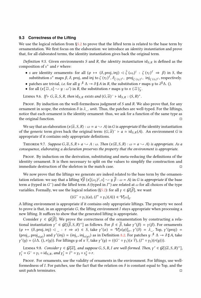
9.3 Correctness of the Lifting
We use the logical relation from §5.2 to prove that the lifted term is related to the base term by
ornamentation. We first focus on the elaboration: we introduce an identity instantiation and prove
that, for all elaborated terms, the identity instantiation gives back the original term.
Definition 9.5. Given environments S and R, the identity instantiation idS,R is defined as the
composition of s+ and r where:
• s are identity ornaments: for all (φ 7→ (δ , proj, inj) � ˆζ (ωi )i
: ζ (τℓ )ℓ ⇒ β ) in S , the
substitution s+ maps β , δ , proj, and inj to ζ (τℓ )ℓ, δζ (τℓ )ℓ , projζ (τℓ )ℓ , injζ (τℓ )ℓ , respectively.
• patches are trivial, i.e. for all y :♯ ∆→ δ ♯A in R, the substitution r maps y to λ♯∆. ().
• for all (x[ω , s] ; y : ω ′) in R, the substitution r maps y to x (ω )−S .
Lemma 9.6. If ⊢ G,α , S,R, then idS,R exists and (G,α )− ⊢ idS,R : (S,R)+.
Proof. By induction on the well-formedness judgment of S and R. We also prove that, for any
ornament in scope, the extension δ is λ_. unit. Thus, the patches are well-typed. For the liftings,notice that each ornament is the identity ornament: thus, we ask for a function of the same type as
the original function. □
We say that an elaboration (x⟨α , S,R⟩ : ω = a ; A) inG is appropriate if the identity instantiation
of the generic term gives back the original term: (G,α )− ⊢ a ≃ idS,R (A). An environment G is
appropriate if it contains only appropriate definitions.
Theorem 9.7. Suppose G,α , S,R ⊢ a ; A : ω. Then (x⟨α , S,R⟩ : ω = a ; A) is appropriate. As aconsequence, elaborating a declaration preserves the property that the environment is appropriate.
Proof. By induction on the derivation, substituting and meta-reducing the definitions of the
identity ornament. It is then necessary to split on the values to simplify the construction and
immediate destruction of the skeleton in the match case. □
We now prove that the liftings we generate are indeed related to the base term by the ornamen-
tation relation: we say that a lifting ∀β (x[(ωj )j , s] ; y β : ω = A) in G is appropriate if the base
term a (typed in G−) and the lifted term A (typed in I+) are related at ω for all choices of the type
variables. Formally, we use the logical relation (§5.2): for all γ ∈ G[β], we want((G− ◦ γ1) (a), (I
+ ◦ γ2) (A))∈ V[ω]γ
A lifting environment is appropriate if it contains only appropriate liftings. The property we need
to prove is that, in an appropriateG , the lifting environment I stays appropriate when processing a
new lifting. It suffices to show that the generated lifting is appropriate.
Consider γ ∈ G[β]. We prove the correctness of the ornamentation by constructing a rela-
tional instantiation γ ′ ∈ G[(β, S,R)+] as follows. For β ∈ β , take γ ′(β ) = γ (β ). For ornaments
(φ 7→ (δ , proj, inj) � _ : τ ⇒ α ) ∈ S , take γ ′(α ) = V[s (φ)]γ , γ′(δ ) = λ_. Top, γ ′(proj) =
(projτ , projs (φ ) ) and γ′(inj) = (injτ , injs (φ ) ) as in Definition 8.2. For patches y :
♯ ∆ → δ ♯A, take
γ ′(y) = (λ∆. (), r (y)). For liftings y of x τ , take γ ′(y) = ((G− ◦ γ1) (x τ ), (I+ ◦ γ2) (r (y))).
Lemma 9.8. Consider γ ∈ G[α], and suppose G, S,R, I are well-formed. Then, γ ′ ∈ G[(α , S,R)+],
γ ′1= G− ◦ γ1 ◦ idS,R , and γ ′2 = I+ ◦ γ2 ◦ s
+S ◦ r .
Proof. For ornaments, use the validity of ornaments in the environment. For liftings, use well-
formedness of I . For patches, use the fact that the relation on δ is constant equal to Top, and the
unit patch terminates. □

Then, we can instantiate the generic term with γ ′. On the left-hand side we obtain a term
equivalent to the base term, and on the right-hand side a term equivalent to the lifted term (because
simplification preserves equivalence). Both terms are related by the relationV[s (ω)]γ . Thus wededuce correctness of the lifting process:
Theorem 9.9 (Correctness of lifting). Suppose I is appropriate, and consider a lifting request s .If G; I ⊢ s ⇒ I ′, then I ′ is appropriate.
Proof. Let us consider the rule Lifting. First, (s+S ◦ r ) (A) is well-typed in an equality-free
environment, and thus simplifies to an ML term, preserving equality (and thus the logical relation).
Consider γ ∈ Gk [β]. We have to prove:
((G− ◦ γ1) (a), (I+ ◦ γ2 ◦ s
+S ◦ r ) (A)) ∈ V[s (ω)]γ
Consider γ ′ defined as above. We can rewrite a to idS,R (A) by the identity instantiation property of
G . Thus, (G− ◦ γ1) (a) = γ′1(a). By definition, (I+ ◦ γ2 ◦ s
+S ◦ r ) (A) = γ
′2(a). Suppose S gives the type
variables αi as lifted types of the ornament variables φi . Then,
V[s (ω)]γ = V[ω[φi ← s (φi )]i]γ
= V[ω]γ [φi←V[s (φi )]γ ]i
= V[ω+S ]γ [αi←V[s (φi )]γ ]i
= V[ω+S ]γ ′
Thus, we have to prove (γ ′1(A),γ ′
2(A)) ∈ V[ω+S ]ρ . This is true by the fundamental lemma, because
γ ′ ∈ Gk [(β , S,R)+] and (β , S,R)+ ⊢ A : ω+S . □
In the case of strictly positive datatypes and first-order functions, this result can be translated
to the coherence property of ornaments [Dagand and McBride 2014]. We can define a projection
function that projects the whole datatype at once (rather than incrementally as with the projfunction), e.g. the length function for natlist α . Then, the relation expressed by natlist α between
a1 and a2 is simply a1 = length a2 (up to termination). The statement that append is a lifting of
add at natlist α → natlist α → natlist α can then be translated (again, up to termination) to the
fact that, for all a1,a2, length (append a1 a2) = add (length a1) (length a2).
9.4 Termination via the Inverse Relation
In order to prove that, when the patches terminate, the lifted term does not terminate less that the
base term, we need to use the relation the other way, with the base term on the right and the lifted
type on the left.
The relation is defined similarly. The only difference is that the Top relation, in the first case,
relates any term on the base side (i.e. the left) to a non-terminating term on the lifted side (i.e. the
right), while the reversed Top relates any terminating term on the lifted side (i.e. this time, the left)
to any term on the base side (i.e. the right). Thus, the difference occurs at instantiation: we need to
prove that the patches terminate to inject them in the relation.
10 DISCUSSION
10.1 Implementation and Design Issues
Our prototype tool for refactoring ML programs using ornaments closely follows the structure
outlined in this paper: programs are first elaborated into a generic term, stored in an elaboration
environment and then instantiated and simplified in a separate phase. From our experience, this
principled approach is more modular and robust than an attempt to go directly from base terms to
ornamented terms. Of course, our prototype also performs inference during elaboration, while we

have only presented elaboration as a checking relation. Inference is a rather orthogonal issue and
does not raise any difficulty.
The prototype is a proof of concept that only accepts programs in a toy language. Porting the
implementation to a real language, such as OCaml, would allow to demonstrate the benefits of
ornamentation on real, large cases. We believe that instances of pure refactoring would already be
very useful to the programmer, even though it is just a small subset of the possibilities.
As presented, elaboration abstracts over all possible ornamentation points, which requires to
specify many identity ornaments and corresponding trivial patches, while many datatypes may
never be ornamented. For example, refactoring a library may need a specific ornament for one
type and the identity ornament for all others. We already allow wildcard on occurrences to apply
the identity ornaments by default. We could also use global rules, to avoid repeating local rules.
We could also avoid generating the ornamentation points in the generic lifting that are known in
advance to be always instantiated to the identity ornament. This information could be user-specified,
or be inferred by scanning all ornament definitions prior to elaboration.
The lifting process, as described, only operates onML terms restricted to shallow patternmatching
and where constructors are only applied to variables. To meet these restrictions we preprocess
terms, turning deep pattern matching into shallow pattern matching, and lifting the arguments
of constructors into separate let bindings. This does not preserve the structure of the original
program and creates unnatural looking terms as output. To recover a term closer to the original
one, we mark the bindings we introduced and substitute them back afterwards. When applying
this transformation, we keep the evaluation order of the arguments even if they are permuted.
Thus our implementation should preserve effects and their ordering. We use a similar strategy
for deep pattern matching. During compilation to shallow pattern matching, we annotate the
generated matches with tags that are maintained during the elaboration and, whenever possible,
we merge back pattern matchings with identical tags after elaboration. This seems to work well,
and a primitive treatment of deep pattern matching does not seem necessary andould be more
involved, so we currently do not feel the need for such an extension.
Pattern matching clauses with wildcards may be expanded to multiple clauses with different head
constructors. For the moment we only factor them back in obvious cases, but we could use tags
to try to merge all clauses in the lifted code that originate from the same clause in the base code.
These transformation phases introduce auxiliary variables. Some of these bindings will eventually
be expanded, but some will remain in the lifted program. Before printing, we select names derived
from the names used in the original program. This seems to be enough to generate readable terms.
10.2 Polymorphic Let Bindings
Currently, in a pre-elaboration pass, all local polymorphic let-bindings are duplicated into a sequence
of monomorphic let for each usage point. This does not reduce the expressivity of the system
—assuming, as [Vytiniotis et al. 2010], that they are sufficiently rare (see to avoid exponential
behavior. This transformation requires the user to instantiate what appears to be the same code
multiple times. On the other hand, it is useful because it allows lifting a local definition differently
for different usage points.
The duplicated local definitions could be tagged and shared back after ornamentation if their
instantiations are identical. Another approach would be to allow the user to provide several
ornamentations at the definition point, and then choose one ornamentation at each usage point.
From a theoretical point of view, this is equivalent to λ-lifting and extruding the definition to the
toplevel: we can then use our mechanism for lifting references to global definition and fold the
definition back in the term before printing it out. It would also be possible to allow a local definition
to be ornamented with polymorphic ornaments, i.e. ornaments polymorphic on a type parameter.

This would not solve the problem of using different ornaments for different usage points, but would
allow polymorphic recursion—which is not allowed in our current presentation.
10.3 Lifting
For convenience, we do not require that all parameters be instantiated when lifting a term: we infer
some ornaments and liftings and automatically fill-in patches that return unit. We also provide a
way to specify a default ornament for a type. These simple strategies seem to work well for small
examples, but it remains to see if they also scale to larger examples with numerous ornamentation
points. Our view is that inferring patches is an orthogonal issue that can be left as a post-processing
pass, with several options that can be studied independently but also combined. One possibility is
to use code inference techniques such as implicit parameters [Chambard and Henry 2012; Devriese
and Piessens 2011; Scala 2017; White et al. 2014], which could return three kinds of answers: a
unique solution, a default solution, i.e. letting the user know that the solution is perhaps not unique,
or failure, as illustrated in §2.3.
In our presented, we implicitly assume that all the code is available to the ornamentation tool.
Ornamentation schemes can be derived for the whole program, ornamented at once. In realistic
scenarios, programs are written in a modular way. We could generalize and then instantiate whole
modules, and store the resulting environments in an ornamentationnterface file describing the
relation between a base module and its lifting. Modular ornamentation could be applied to libraries:
when releasing a new interface-incompatible version of a library, a maintainer could distribute
an ornamentation specification allowing clients of the library to automatically migrate their code,
leaving holes only at the points requiring user input.
10.4 Semantic Issues
Our approach to ornamentation is not semantically complete: we are only able to generate lift-
ings that follow the syntactic structure of the original program, instead of merely following its
observable behavior. Most reasonable liftings seem to follow this pattern. Syntactic lifting seems
to be rather predictable and intuitive and leads to quite natural results. This restriction also helps
with automation by reducing the search space. Still, it would be interesting to find a less syntactic
description of which functions can be reached by this method.
We could also consider preprocessing source programs prior to ornamentation. Indeed, η-expansion or unfolding of recursive definitions could provide more opportunities for ornamentation
(e.g. in §??). In the cases we observed, the unfolding follows the structure of an ornament. Hence, it
would be interesting to perform the unfolding on demand during the instantiation process.
The correctness result we give for lifting only gives weak guarantees with respect to termination:
since the logical relation relates a non-terminating term on the right-hand side to any term on the
left-hand side, a diverging term is an ornamentation of any term. Using the inverse relation, can
prove a stronger property: if the patches always terminate, the lifting terminates exactly when
the base term terminates.However, we would like an even more precise result: if a lifting does not
terminate while the base term terminates, it can only be because of looping inside the code given
by a patch.
We have described ornaments as an extension of ML, equipped a call-by-value semantics, but
only to have a fixed setting: our proposal should apply seamlessly to core Haskell. Our presentation
of ornamentation ignores effects, as well as the runtime complexity of the resulting program. A
desirable result would be that an ornamented program produces the same effects as the original
program, save for the effects performed in patches. Similarly, the complexity of the ornamented
program should be proportional to the complexity of the original one, save for the time spent in
patches.

10.5 Future Work
Programming with generalized algebraic datatypes (GADT) requires writing multiple definitions
of the same type holding different invariants. GADT definitions that only add constraints could
be considered ornaments of regular types, which was one of the main motivations for introducing
ornaments in the first place [Dagand and McBride 2014]. It would then be useful to automatically
derive, whenever possible, copies of the functions on the original type that preserve the new
invariants. Extending our results to the case of GADTs is certainly useful but still challenging future
work. Besides issues with type inference, GADTs also make the analysis of dead branches more
difficult. A possible approach with our current implementation is to generate the function, ignoring
the constraints, and hoping it typechecks, but a more effective strategy will probably be necessary.
Although dependently typed, the meta-language mML is in fact quite restrictive. It must fulfill
two conflicting goals: be sufficiently expressive to make the generic lifting well-typed, but also
restrictive enough so that elaborated programs can be reduced and simplified back to ML. Hence,many extensions of ML will require changing the language eML as well, and it is not certain that
the balance will be preserved, i.e. that lifted program will remain typable in the source language.
The languages eML andmML have only been used as intermediate languages and are not exposed
to the programmer. We wonder whether they would have other useful applications for other
program transformations or for providing the user with some meta-programming capabilities. For
example, eML is equipped to keep track of term equalities during pattern matching and could
perhaps have applications in other settings. Similarly, one might consider exposing mML to the
user to let her write generic patches that could be instantiated as needed at many program points.
Ornaments can be composed in multiple ways. Applying the effects of two ornaments consecu-
tively (lifting one type to another one, and lifting the lifted type again to a third type) can be done by
re-lifting an already lifted definition. An interesting direction is to combine the information added
by two ornaments into a datatype representing the base type and both ornamentations [Dagand
and McBride 2013; Ko and Gibbons 2013]. Lifting could then similarly be composed to liftings
along the combined ornament. This could be especially useful with GADTs: one could build a new
datatype by combining two invariants established independently and obtain liftings by combining
two independent liftings. Finally, it would be interesting to consider other transformations of
datatypes, and in particular, deornamentation: instead of adding information to existing datatypes,
deornamentation removes information from a datatype and adapts the functions operating on the
original datatype so that they can operate on its impoverished version.
11 RELATED WORK
Ornaments have been recently introduced by [Dagand and McBride 2013, 2014; McBride 2011]
in the context of dependently typed languages, where they can be encoded instead of treated as
primitive. In this context, Ko and Gibbons [2016] describe a different way to handle higher-order
ornaments without using logical relations. We first considered applying ornaments to an ML-likelanguage in [Williams et al. 2014].
Type-Theory in Color [Bernardy and Guilhem 2013] is another way to understand the link
between a base type and a richer type. Some parts of a datatype can be tainted with a color
modality: this allows tracing which parts of the result depend on the tainted values and which
are independent. Terms operating on a colored type can then be erased to terms operating on the
uncolored version, which would correspond to the base term. This is internalized in the type theory:
in particular, equalities involving the erasure hold automatically. This is the inverse direction from
ornaments: once the operations on the ornamented datatype are defined, the base functions are
automatically derived, as well as a coherence property between the two implementations. Moreover,
the range of transformations supported by type theory in color is more limited: it only allows field
erasure, but not, for example, to rearrange a products of sums as a sum of products
Programming with GADTs may require defining one base structure and several structures with
some additional invariants, along with new functions for each invariant. Ghostbuster [McDonell
et al. 2016] proposes a gradual approach to porting functions to GADTs with richer invariants, by
allowing as a temporary measure to write a function against the base structure and dynamically
checking that it respects the invariant of the richer structure, until the appropriate function is
written.
Najd and Peyton-Jones [2016] also observe that one often needs many variants of a given data
structure (typically an abstract syntax tree), and corresponding functions for each variant. They
propose a programming idiom to solve this problem: they create an extensible version of the type,
and use type families to determine from an extension name what information must be added to
each constructor. In this approach, the type of the additional information only depends on the
constructor, while our type-level pattern matching allows depending on the information stored in
the already-present fields. This approach uses only existing features of GHC, avoiding a separate
pre-processing step and allowing one to write generic functions that operate on all decorations
of a tree. On the other hand, the programmer must pay the runtime cost of the encoding even
when using only the undecorated tree. The encoding of extensible trees scales naturally to GADTs.
Interestingly, this idiom and ornaments are largely orthogonal features with some common use
case (factoring operations working on several variants of the same datatype) and might hopefully
benefit from one another.
Our mML language is equipped with rudimentary meta-programming facilities, by separating a
meta-abstraction from the ML abstraction. Its main distinguishing features from usual approaches
to meta-programming in ML (such as Kiselyov [2014]) is its ability to embed eML and transform
equalities, allowing simplification of partial pattern matchings.
Ornamentation is a form of code refactoring on which there is a lot of literature, but based on
quite different techniques and rarely supported by a formal treatment. It has however not been
much explored in the context of ML-like languages.
Views, first proposed by Wadler [Wadler 1986] and later reformulated by Okasaki [Okasaki
1998] have some resemblance with isomorphic ornaments. They allow several interchangeable
representations for the same data, using isomorphism to switch between views at runtime whenever
convenient. The example of location ornaments, which allows to program on the bare view while
the data leaves in the ornamented view, may seem related to views, but this is a misleading intuition.
In our case, the switch between views is at editing time and nothing happens at runtime where
only the ornamented core with location is executed. In fact, this runtime change has a runtime
cost, which is probably one of the reasons why the appealing concept of views never really took
off. Lenses [Foster et al. 2007] also focus on switching representations at runtime.
The ability to switch between views may also be thought of as the existence of inverse coercions
between views. Coercions may be considered as the degenerate of views in the non-isomorphic
case. But coercions are not more related to ornaments than views—for similar reasons.
CONCLUSION
We have designed and formalized an extension of ML with ornaments. We have used logical
relations as a central tool to give a meaning to ornaments, to closely relate the ornamented and
original programs, and to guide the lifting process. We believe that this constitutes a solid, but
necessary basis for using ornaments in programming. This is also a new use of logical relations
applied to type-based program refactoring.

Ornaments seem to have several interesting applications in an ML setting. Still, we have so far
only explored them on small examples and more experiment is needed to understand how they
behave on large scale programs. We hope that our proof-of-concept prototype could be turned into
a useful, robust tool for refactoring ML programs. Many design issues are still open to move from a
core language to a full-fledged programming language. More investigation is also needed to extend
our approach to work with GADTs.
A question that remains unclear is what should be the status of ornaments: should they become a
first-class construct of programming languages, remain a meta-language feature used to preprocess
programs into the core language, or a mere part of an integrated development environment?
Our principled approach with a posteriori abstraction of the source term revealed very beneficial
for ornaments and we imagine that it could also be used for other forms of program transformations
beyond ornaments that remain to be explored.
REFERENCESJean-Philippe Bernardy and Moulin Guilhem. 2013. Type-theory in color. In International Conference on Functional Program-
ming. 61–72. https://doi.org/10.1145/2500365.2500577
Pierre Chambard and Grégoire Henry. 2012. Experiments in generic programming: runtime type representation and
implicit values. Presentation at the OCaml Users and Developers meeting, Copenhagen, Denmark. (sep 2012). http:
//oud.ocaml.org/2012/slides/oud2012-paper4-slides.pdf
Pierre-Évariste Dagand and Conor McBride. 2013. A Categorical Treatment of Ornaments. In 28th Annual ACM/IEEE
Symposium on Logic in Computer Science, LICS 2013, New Orleans, LA, USA, June 25-28, 2013. IEEE Computer Society,
530–539. https://doi.org/10.1109/LICS.2013.60
Pierre-Évariste Dagand and Conor McBride. 2014. Transporting functions across ornaments. J. Funct. Program. 24, 2-3
(2014), 316–383. https://doi.org/10.1017/S0956796814000069
Dominique Devriese and Frank Piessens. 2011. On the Bright Side of Type Classes: Instance Arguments in Agda. In
Proceedings of the 16th ACM SIGPLAN International Conference on Functional Programming (ICFP ’11). 143–155. https:
//doi.org/10.1145/2034773.2034796
J. Nathan Foster, Michael B. Greenwald, Jonathan T. Moore, Benjamin C. Pierce, and Alan Schmitt. 2007. Combinators for
bidirectional tree transformations: A linguistic approach to the view-update problem. ACM Transactions on Programming
Languages and Systems 29, 3 (May 2007), 17. https://doi.org/10.1145/1232420.1232424
Oleg Kiselyov. 2014. The Design and Implementation of BER MetaOCaml. Springer International Publishing, Cham, 86–102.
https://doi.org/10.1007/978-3-319-07151-0_6
Hsiang-Shang Ko. 2014. Analysis and synthesis of inductive families. DPhil dissertation. University of Oxford.
Hsiang-Shang Ko and Jeremy Gibbons. 2013. Modularising inductive families. Progress in Informatics 10 (2013). https:
//doi.org/doi:10.2201/NiiPi.2013.10.5
Hsiang-Shang Ko and Jeremy Gibbons. 2016. Programming with ornaments. Journal of Functional Programming 27 (2016).
https://doi.org/10.1017/S0956796816000307
Conor McBride. 2011. Ornamental Algebras, Algebraic Ornaments. (2011). https://personal.cis.strath.ac.uk/conor.mcbride/
pub/OAAO/LitOrn.pdf
Trevor L. McDonell, Timothy A. K. Zakian, Matteo Cimini, and Ryan R. Newton. 2016. Ghostbuster: A Tool for Simplifying
and Converting GADTs. In Proceedings of the 21st ACM SIGPLAN International Conference on Functional Programming
(ICFP 2016). ACM, New York, NY, USA, 338–350. https://doi.org/10.1145/2951913.2951914
Shayan Najd and Simon Peyton-Jones. 2016. Trees that grow. JUCS (2016). https://www.microsoft.com/en-us/research/
wp-content/uploads/2016/11/trees-that-grow-2.pdf
Chris Okasaki. 1998. Views for Standard ML. In In SIGPLAN Workshop on ML. 14–23.
Scala. 2017. Implicit Parameters. Scala documentation. (2017). https://docs.scala-lang.org/tour/implicit-parameters.html
Dimitrios Vytiniotis, Simon Peyton Jones, and Tom Schrijvers. 2010. Let Should Not Be Generalised, In Proceedings of the
5th ACM SIGPLAN Workshop on Types in Language Design and Implementation. https://www.microsoft.com/en-us/
research/publication/let-should-not-be-generalised/
Philip Wadler. 1986. Views: A way for pattern matching to cohabit with data abstraction. (1986).
Leo White, Frédéric Bour, and Jeremy Yallop. 2014. Modular implicits. In Proceedings ML Family/OCaml Users and Developers
workshops, ML/OCaml 2014, Gothenburg, Sweden, September 4-5, 2014. 22–63. https://doi.org/10.4204/EPTCS.198.2
Thomas Williams, Pierre-Évariste Dagand, and Didier Rémy. 2014. Ornaments in practice. In Proceedings of the 10th ACM
SIGPLAN workshop on Generic programming, WGP 2014, Gothenburg, Sweden, August 31, 2014, José Pedro Magalhães and

Tiark Rompf (Eds.). ACM, 15–24. https://doi.org/10.1145/2633628.2633631
Thomas Williams and Didier Rémy. 2017. A Principled Approach to Ornamentation in ML. Research Report RR-9117. Inria.
https://hal.inria.fr/hal-01628060