reliability problems in earthquake engineering
TRANSCRIPT

Reliability Problems in Earthquake Engineering
J. E. Hurtado
Monograph CIMNE IS-63, 2010

Monografías de Ingeniería Sísmica Editor A. H. Barbat
Reliability Problems in Earthquake Engineering
J. E. Hurtado
Monograph CIMNE IS-63, 2010

CENTRO INTERNACIONAL DE MÉTODOS NUMÉRICOS EN INGENIERÍA Edificio C1, Campus Norte UPC Gran Capitán s/n 08034 Barcelona, Spain MONOGRAFÍAS DE INGENIERÍA SÍSMICA Editor A. H. Barbat ISSN: 1134-3249 RELIABILITY PROBLEMS IN EARTHQUAKE ENGINEERING Monografía CIMNE IS63 Los autores ISBN: 978-84-96736-86-3 Depósito legal: B-18792-2010

Introduction
This monograph deals with the problem of reliability analysis in the field of Earth-quake Engineering. Chapter 1 is devoted to a summary of the most widely usedreliability methods, with emphasis on Monte Carlo and solver surrogate techniquesused in the subsequent chapters. Chapter 2 presents a discussion of the MonteCarlo from the viewpoint of Information Theory. Then, a discussion is made inChapter 3 on the selection of random variables in Earthquake Engineering. Next,some practical methods for computing failure probabilities under seismic loads arereported in Chapter 4. Finally, a method for reliability-based design optimizationunder seismic loads is presented in Chapter 5.
1

2 Reliability problems in Earthquake Engineering
Contents
1 Basic concepts of structural reliability 5
1.1 Performance and limit-state functions . . . . . . . . . . . . . . . . . 5
1.2 Methods based on the limit-state function . . . . . . . . . . . . . . 8
1.3 Transformation of basic variables . . . . . . . . . . . . . . . . . . . 9
1.4 FORM and SORM . . . . . . . . . . . . . . . . . . . . . . . . . . . 12
1.4.1 Basic equations . . . . . . . . . . . . . . . . . . . . . . . . . 12
1.4.2 Discussion . . . . . . . . . . . . . . . . . . . . . . . . . . . . 14
1.5 Monte Carlo methods . . . . . . . . . . . . . . . . . . . . . . . . . . 16
1.5.1 Importance Sampling . . . . . . . . . . . . . . . . . . . . . . 18
1.5.2 Directional Simulation . . . . . . . . . . . . . . . . . . . . . 22
1.5.3 General characteristics of simulation methods . . . . . . . . 24
1.6 Relevance of solver-surrogate building . . . . . . . . . . . . . . . . . 25
1.7 Solver-surrogate methods . . . . . . . . . . . . . . . . . . . . . . . . 26
1.7.1 Response Surface Method . . . . . . . . . . . . . . . . . . . 26
1.7.2 Neural Networks and Support Vector Machines . . . . . . . 29
1.7.3 Characteristics of the Response Surface Method . . . . . . . 32
1.8 Regression and Classification . . . . . . . . . . . . . . . . . . . . . . 38
1.9 FORM and SORM approximations with Statistical Learning devices 41
1.10 Methods based on the performance function . . . . . . . . . . . . . 42
2 Information characteristics of Monte Carlo simulation 45
2.1 Introduction . . . . . . . . . . . . . . . . . . . . . . . . . . . . . . . 45
2.2 Some concepts of Information Theory . . . . . . . . . . . . . . . . . 48
2.3 Information characterization of Monte Carlo simulation . . . . . . . 51
2.4 Application examples . . . . . . . . . . . . . . . . . . . . . . . . . . 56
3

4 Reliability problems in Earthquake Engineering
3 Seismic random variables 61
3.1 Introduction . . . . . . . . . . . . . . . . . . . . . . . . . . . . . . . 613.2 Robust and Reliability-based design options . . . . . . . . . . . . . 633.3 Stochastic models of seismic action . . . . . . . . . . . . . . . . . . 653.4 Fundamentals of random vibration analysis . . . . . . . . . . . . . . 703.5 Practical computation of seismic robustness . . . . . . . . . . . . . 74
3.5.1 Moments of maximum response . . . . . . . . . . . . . . . . 743.5.2 Unconditional moments . . . . . . . . . . . . . . . . . . . . 76
4 Practical computation of seismic reliability 81
4.1 Introduction . . . . . . . . . . . . . . . . . . . . . . . . . . . . . . . 814.2 Backward Sampling with Delaunay tessellation . . . . . . . . . . . . 824.3 Improving estimates with the Total Probability Theorem . . . . . . 85
4.3.1 Backward stratified sampling . . . . . . . . . . . . . . . . . 884.3.2 Application to a base isolated building . . . . . . . . . . . . 92
5 Reliability-based seismic optimization 99
5.1 Introduction . . . . . . . . . . . . . . . . . . . . . . . . . . . . . . . 995.2 A new algorithm for generating SVM training samples . . . . . . . 101
5.2.1 Example 5.1. Two dimensional function . . . . . . . . . . . 1085.2.2 Example 5.2. Two dimensional function with small Pf . . . . 110
5.3 Methodology for RBDO . . . . . . . . . . . . . . . . . . . . . . . . 1125.4 Earthquake Engineering application example . . . . . . . . . . . . . 116
5.4.1 Stochastic spectrum . . . . . . . . . . . . . . . . . . . . . . 1185.4.2 Discussion on a base isolated building case . . . . . . . . . . 1205.4.3 RBDO of a base isolated building . . . . . . . . . . . . . . . 122
5.5 Final remarks . . . . . . . . . . . . . . . . . . . . . . . . . . . . . . 127

Chapter 1
Basic concepts of structural
reliability
This introductory chapter summarizes some well-established concepts and methodsfor structural reliability computations for the better understanding of the discus-sions and ideas exposed in the following chapter for the specific field of EarthquakeEngineering.
1.1 Performance and limit-state functions
The main problem in stochastic mechanics is the estimation of the probabilitydensity function of one or several structural responses. If the case under analysisis a dynamical one, then the aim would be to calculate the evolution of suchdensities. This kind of problem can be termed full probabilistic analysis. A derived,more practical problem is to find a specific probability of exceeding a responsethreshold that can be considered critical for the serviceability or the stability ofthe system. This is the reliability analysis. Notice that, in principle at least,the second problem could be solved after the first, as the probability of failurecan eventually be obtained by integration of the probability density function ofthe observed response. However, most reliability methods developed in the lastdecades attempt to estimate directly the failure probability or related reliability
5

6 Reliability problems in Earthquake Engineering
indices without calculating first the response density function for reasons explainedin the sequel.
In the reliability problem the input random variables (called also basic vari-
ables) are collected in a set x, whose deterministic counterpart is the vector x.This defines the input space. Let us define a performance function g(x) that in-corporates both the response r(x) and a critical threshold for it, r, in such away that g(x) > 0 means that the sample x is in the safe domain and g(x) < 0implies failure. Hence there is a boundary g(x) = 0 between the two domainsS = x : g(x) > 0 and F = x : g(x) < 0 that is termed limit-state function.
For structural components, the performance function writes
g(x) = S(x) − R(x) (1.1)
where x = [x1, x
2, . . . , xd] is the vector of d input variables, S(x) is a load effect
on the component and R(x) the strength capacity to withstand it. In the caseof complex structures the performance function is given only implicitly through afinite element (or similar) code in the form
g(x) = r − r(x) = 0 (1.2)
in which r(x) the implicit function and r is a critical threshold for the response r(·)whose surpassing indicates failure. Notice, however, that for structural componentsthe load effects S(x) in Eq. (1.1) depend on the overall structural response andhence they are also known only implicitly (The only exception to this rule are thesimple statically determinate structures, as is well known). As a consequence, acorrect probabilistic description of the load effects on each component also passesthrough several finite element solutions.
For solving the above reliability problem two kinds of methods have been de-veloped, according to which of the two functions is used as a reference. In themethods based on the limit-state function the shape of the function g(x) = 0 inthe x−space is of paramount importance, since the purpose is to compute theintegral
Pf =
∫
g(x)≤0
px(x)dx (1.3)
that yields the probability of failure. Here px(x) is the joint probability of therandom variables. In this family we have the methods which are most widelyapplied, such as those based on the Taylor expansion of the performance function
Basic concepts 7
(FORM and SORM) and some variants of Monte Carlo methods (ImportanceSampling, Directional Simulation, etc). In the methods based on the performance
function one observes the random variable g(x) and defines the failure probabilityas
Pf = P [g ≤ 0] (1.4)
Notice that to this purpose it is not necessary to consider the form of the limit-state function g(x) = 0 in the x space. This has an important advantage fromthe practical viewpoint, which is that the probabilities of failure correspondingto several limit-states can be obtained at the same computational cost that fora single one, because it is only a matter of observing several responses g
i, i =
1, 2, . . . instead of one. In principle, any stochastic mechanics method giving theprobability density function of the observed response, normally through momentsor cumulants, can be used for estimating the reliability by integration. Although,most reliability methods published to-date belong to the former category. This isdue to the fact that in this approach there are some bye-product measures suchas reliability indices and, in particular, design points that provide useful insightinto the structural reliability problem, that are not obtained with the performancefunction approach. This is especially true in the particular case of incompletestatistical information.
Methods of analysis
Analytic (Taylor-based)
FORM SORM
Synthetic (Monte Carlo)
Direct Substitution
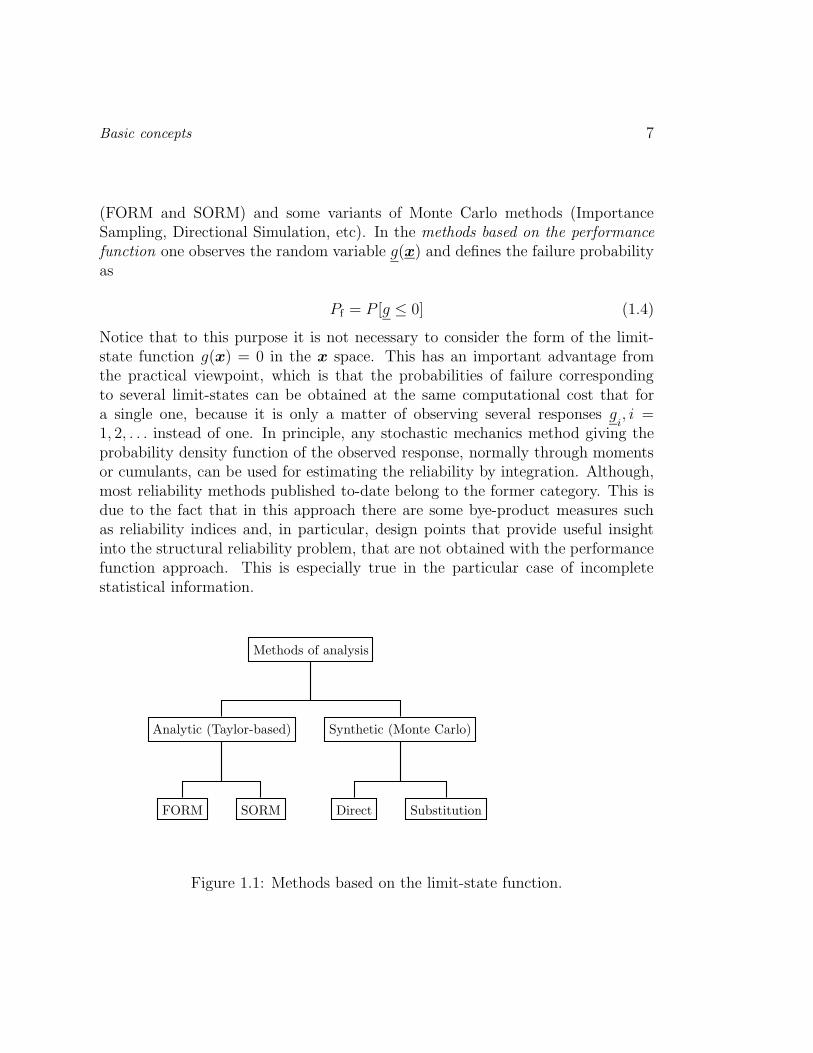
Figure 1.1: Methods based on the limit-state function.

8 Reliability problems in Earthquake Engineering
1.2 Methods based on the limit-state function
The methods based on the limit-state function that have been proposed so far inthe international literature can be grouped into two general families which can benamed as analytic and synthetic, according to whether the random variable set x
and its effects are treated with the tools of Probability Theory or with those ofStatistics (see Fig. 1.1). In the first case we have two families of methods based onthe Taylor-series expansion of the limit state function, which are known as FORM(First-Order) and SORM (Second-Order Reliability Method). The FORM methodrequires information on the value of the performance function and its gradient inthe vicinity of the so-called design point and the SORM method needs also theknowledge of the second-order derivatives. In the second case, sample sets of thebasic variables are generated and processed by a numerical solver of the structuralmodel in order to obtain a population of structural responses over which statisticalanalyses can be conducted (Monte Carlo simulation). An important consequenceof this approach, not sufficiently stressed nor evaluated in many papers on thesubject, is that the failure probability becomes a random variable with normallya high coefficient of variation.
Monte Carlo
Substitution
DOE
SL
Regression
Classification
Direct
Descriptive
Variance reduction
Figure 1.2: Taxonomy of Monte Carlo methods.

Basic concepts 9
Monte Carlo methods in structural reliability comprehend those oriented to anoverall statistical description of the response, such as Latin Hypercube ([1]; [2]; [3])or Descriptive Sampling [4], and those specially purported at solving the integral(1.3), which are commonly known as variance reduction methods. These includeImportance Sampling ([5]; [6]), Directional Sampling [7] and Subset Simulation[8]. Advanced versions of the descriptive methods, however, have been recentlyproposed for the reliability problem [9]. All these methods can be applied either tothe numerical solver of the structural model to obtain the samples of the structuralresponses (direct simulation) or to a suitable solver surrogate thereof (Fig. 1.2). Inthis latter case a simple function that yields estimates of the structural response ofinterest in the reliability analysis is calculated. The above mentioned randomnessof the failure probability points out the importance of this alternative, because evenwhen applying variance-reduction methods there is a need of repeating the entiresimulation some times in order to produce an average of the failure probability orthe reliability index, because the coefficient of variation of the failure probabilitytends to be the higher, the lower the target probability [10]. If the solver issubstituted by an approximating function, these additional runs and a large partof the first one can be performed without resort to the finite element code butusing the function instead.
The construction of a surrogate of the finite-element solver has been attemptedin the last decades by means of the Response Surface Method (RSM) developed inthe field of Design of Experiments (DOE) (see e.g. [11], [12]). In recent yearsit has been proposed to develop alternative solver-surrogates using StatisticalLearning (SL) techniques such as Neural Networks or Support Vector Machines,which emerge as alternatives to such purpose with several distinguishing advan-tages [13, 14, 15, 16]. One of them is the possibility of approaching the reliabilityproblem either with regression or with classification tools, as shown later in thischapter.
After introducing these classification of the reliability methods, a summary oftheir basic traits and limitations will be examined in the next paragraphs.
1.3 Transformation of basic variables
The application of some reliability methods, such as FORM and SORM, requiresthat the basic variable vector x, defined by its joint density function or an approx-imate model thereof, be transformed into a set of independent Normal variables u.Such transformations are also very useful when applying Statistical Learning tools.

10 Reliability problems in Earthquake Engineering
This is due to the fact that some of these learning devices employ some specialfunctions that are active in a limited range and hence it is convenient to standard-ize the input variables before training them. For this reason it is important toexamine briefly some standardization techniques.
The transformation of the basic variables from x to u can be performed inseveral ways, according to the available statistical information. For the simple caseof independent Normal variables, the transformation is simply the standardization
ui =xi − µxi
σxi
(1.5)
where µxi, σxi
are respectively the mean and standard deviation of the variable xi.If the variables are correlated, the set u is obtained by a linear transformation ofthe form
u = T (x − µx) (1.6)
where T is a matrix obtained from the Choleski or the spectral decomposition ofthe covariance matrix of the set x. This latter leads to the Principal ComponentAnalysis that allows a direct generation of a small subset of important random vari-ables in a transformed space, thus operating an effective dimensionality reduction.Such an important prerogative is not exhibited by the Choleski decomposition.
In the case where the variables are non-Normal, but are independent, the Nor-mal tail transformation [17] is applicable:
ui = Φ−1(
Pxi(x
i))
(1.7)
Here Pxi(xi) is the distribution of xi and Φ(·) is the standard Normal distribution.
A similar transformation using a non-standard Normal distribution instead of thestandard one is used in the context of FORM algorithms [18].
If the joint density function of all variables is known the Rosenblatt transfor-mation can be applied [19]. The transformation is based on the fact that the multi-variate distribution Px
1,x
2,···xn
(x1, x
2, · · ·xn) is equivalent to Px
1(x
1)Px
2|x
1(x
2|x
1) · · ·
Pxn|x1,x
2,···xn−1
(xn|x1, x
2, · · ·xn−1). Therefore, the transformation can be performed
in the following recursive form:

Basic concepts 11
u1
= Φ−1(
Px1(x
1))
u2
= Φ−1(
Px2|x
1(x
2|x
1))
(1.8)
...
um = Φ−1(
Pxm|x1,x
2,···xm−1
(xm|x1, x
2, · · ·xm−1)
)
where, e.g. Pxi|xj ,xk(xi|xj , xk) is the the conditional distribution of xi given xj and
xk. These functions can only be obtained in some particular cases. Also, it mustbe taken into account that the order of inclusion of the variables in the recursioncan facilitate or complicate the solution.
A more common case is that of variables whose joint density function is notknown (in fact, there are only few continuous multivariate probability models (seee.g. [20]) so that it is not likely that any of them fits the problem in hand), but themarginals and the correlation structure are known. To such situation the Nataftransformation [21] has been found to be very convenient in stochastic mechanics([22];[23]). It consists in transforming the give variables xi to
zi = Φ−1[
Pxi(x
i)]
(1.9)
The set z has zero mean, unit standard deviations and correlation matrix
Rz =
1 ρ12
. . . ρ1,m
ρ21
1 . . . ρ2,m
......
. . ....
. . . . . . . . . 1
(1.10)
in which the correlation coefficients are the solution of the integral equation
ρij =
∫ ∞
−∞
∫ ∞
−∞
(
xi − µi
σi
)(
xj − µj
σj
)
φ2(zi, zj, ρij)dzidzj (1.11)
where φ2
is the standard, two-dimensional Normal density function. Finally, a setof independent Normal variables u can be obtained by the Choleski or spectraldecomposition of matrix Rz . Empirical formulas for estimating ρij after ρij havebeen derived by [22]. The empirical equations can be summarized in the followingunified form:

12 Reliability problems in Earthquake Engineering
Fij = α1+ α
2ηj + α
3η2
j + α4ρ + α
5ρ2 +
α6ρηj + α
7ηi + α
8η2
i + α9ρηi + α
10ηiηj (1.12)
where ρ = ρij. The values of the coefficients can be found in [22]. The maximumerror reported by the authors with respect to the exact values of the ratio is 4.5%.However, most errors are less than one percent.
1.4 FORM and SORM
1.4.1 Basic equations
The First and Second-Order Reliability Methods (FORM and SORM) consist infinding the design point u∗ in a suitable standard space u and substituting theactual performance function by its first- or second-order Taylor expansion aroundthat point. Notice that the transformation from x to u implies that a performancefunction g(u) substitutes g(x). Its second-order Taylor expansion about a pointu+is
g(u).= g(u+) + aT(u − u+) +
1
2(u − u+)TH(u − u+) (1.13)
where a is the gradient vector evaluated at the expansion point
a = ∇g|u+ (1.14)
and H the Hessian matrix
H ij =∂2g
∂ui∂uj
|u+ (1.15)
In FORM the last term in Eq. (1.13) is disregarded and the design point u∗ isthe solution of the optimization problem
minimize β =(
uTu)
1
2
subject to g(u) = 0 (1.16)
The solution of this optimization problem is carried out by mean of iterative tech-niques ([18]). This problem corresponds to finding the shortest distance from the

Basic concepts 13
origin to the limit-state function in the transformed space u so that g(u⋆) = 0.The result is
β = wTu⋆ (1.17)
where
w =a⋆
|a⋆| =∇g(u⋆)
|∇g(u⋆)| (1.18)
is the vector normal to the tangent hyperplane at the design point. Hence theequation of the hyperplane becomes
g(u) = wT(u − u⋆)
= wTu − β (1.19)
which, for comparison with some Statistical Learning equations presented later on,can be put in the form
g(u) = 〈w, u〉 − β (1.20)
where 〈·, ·〉 denotes Euclidean inner product.SORM techniques are based on the above first-order solution. The approxima-
tion of the limit state function (1.13) can be presented in terms of β and u⋆ asfollows:
g(u).= 〈w, u〉 − β +
1
2(u − u⋆)TB(u − u⋆) = 0 (1.21)
where
Bij =1
|∇g(u⋆)|H ij |u⋆ (1.22)
Some approximations to Eq. (1.21) in terms of principal curvatures have beensuggested ([24]; [25]). They are quoted here as they provide useful insight into thereliability problem. By a rotation of the u space to space v such that the designpoint is located in vd the axis, function (1.21) can be recast in the form [24]
−(vd − β) +1
2
(
vd−1
vd − β
)T
A
(
vd−1
vd − β
)
= 0 (1.23)

14 Reliability problems in Earthquake Engineering
where vd−1 = [v1v
2. . . v
d−1]T and A = RBRT, in which R is an orthonormal
matrix with −w as its dth row. Solving the above equation for vd an retainingonly the first two order terms yields
vd = β +1
2vT
d−1Ad−1vd−1 (1.24)
where Ad−1 is formed with the first d − 1 rows and columns of A. By solving theeigenvalue problem of matrix Ad−1, i.e. Ad−1u = κu one obtains the approxima-tion
ud = β +1
2
d−1∑
i=1
κiu2i (1.25)
where the eigenvalues are called principal curvatures. This definition is disputedby [25] who support their approximation in the concept of principal curvature ofdifferential geometry. Their approximation reads
ud = β +1
2R
d−1∑
i=1
u2i (1.26)
where
R =d − 1
K
K =
d∑
i=1
Bjj − wTBw (1.27)
In these equations K is the sum of principal curvatures (according to differentialgeometry) and R is the average principal curvature radius.
1.4.2 Discussion
The calculation of the FORM hyperplane requires the computation of the gradientsof the performance function with respect to all basic variables. This is due to thefact that the problem is formulated as a constrained optimization task. Since theperformance function is normally not given in closed-form, the gradient calculationcan only be performed by finite-difference strategies, which requires a minimumof d + 1 finite element solver calls per iteration point [26]. Since the number of

Basic concepts 15
iterations is of the order of ten, it is evident that the calculation of FORM solu-tions via finite-difference strategies is limited to low dimensionality problems. Thesituation is more severe in the case of SORM because it is necessary to calculatethe elements of the Hessian matrix, which due to symmetry are d(d − 1)/2 + d.Such a involved computation is needed even for applying the approximate SORMtechniques, as Eqs. (1.25) and (1.26) clearly indicate.
For these reason some approaches have been developed for simplifying this task,especially that of FORM. The main trend is the calculation of the gradients at thefinite-element level, by means of the so-called perturbation approach (see e.g. [27]).This implies for instance the calculation of the derivatives of the stiffness matriceswith respect to the basic variables or transformations thereof. This task, however,is also affected by the increase of the dimensionality, because the derivative of aN ×N matrix with respect to a d× 1 vector is a Nd×Nd matrix. Of course, thesituation is more severe for using SORM with such low-level derivatives. Similardimensionality explosions also occur in using other analytical approaches such asthose based on polynomial chaoses ([28]; [29]).
Another aspect that should be considered is the accuracy and stability of theseapproaches. The limitations of FORM in this regard were pointed out by [30].With respect to SORM [31] argues that there are several instances in which thereis an infinite number of SORM quadratic approximations, for a given set of designpoint and principal curvatures, that have associated probabilities running from 0 to1. In words, the SORM results are unstable. Mitteau [31] supports this statementon a single two-dimensional example but a rigorous derivation of its domain ofvalidity is presently lacking. By the same time of Mitteau’s paper, an ample studyon both FORM and SORM was published by [32]. According to the authors theapplicability of FORM is limited to curvatures
|K| ≤ 1
10β(1.28)
and that of SORM to
−0.1(
(2 + 0.6β)√
d − 1 + 3)
≤ |K| ≤ 0.4(√
d − 1 + 3β)
(1.29)
This means that FORM is restricted to cases having very large curvature radius,irrespective to the number of basic variables, and its applicability reduces with theincrease of the reliability as measured by β . On the other hand, SORM showsa different trend. Its applicability increases with the dimensionality and with thefirst-order reliability. However, a previous paper by the authors [25] shows that

16 Reliability problems in Earthquake Engineering
SORM approximate equations are adequate only if the principal curvatures haveall the same sign. If this condition is not met, as in the generalized approximation
ud = β +1
2R
d−1∑
i=1
aiu2i , a < 0, (1.30)
all SORM formulas fail to give the exact results with a large error. This is but aneffect of the rigidity of the SORM model in the sense defined in a next section.
In addition, despite [32] show that SORM has much wider applicability thanFORM, they do not discuss the dimensionality scaling of the number of solvercalls. In fact, it is important to note that in the study it is assumed that thegradients and curvatures have been calculated and, therefore, that the FORMproblem has been solved. Hence, the dimensionality effects on the number ofsolver calls for rendering explicit the limit-state function, that were mentionedabove, should anyhow be considered. As a conclusion, it can be said that besidesthe restrictions for applying FORM and SORM in terms of accuracy, both methodsare applicable only in low-dimensional problems. For a large number of dimensions(a common situation in structural dynamics and stochastic finite element analysis,for instance) these approaches are highly expensive from the computational pointof view.
Given the superiority of SORM over FORM some alternatives to alleviate itscomputational cost have been devised. They consist basically in approximating thegradients and curvatures by fitting a quadratic polynomial using an experimentalplan which in the Response Surface Methodology is called saturated design ([24];[33]). These applications of the Response Surface Method is called point-fittingin the context of SORM analysis. It is illustrated in Fig. 1.3 after the first ofthe quoted references. However, better approximations can be obtained with someStatistical Learning methods as shown in the sequel.
1.5 Monte Carlo methods
In order to review variance reduction Monte Carlo methods, which are the mostcommonly applied in structural reliability, let us first summarize the basic (orcrude) Monte Carlo simulation technique. For estimating the integral
Pf =
∫
F
px(x)dx (1.31)

Basic concepts 17
u1
ud
ud
ud
⋆
β
kβ kβ• •
Figure 1.3: Point-fitting method for SORM approximation (Adapted from [24]).
the domain of integration can be changed to the entire real space using the indicatorfunction
ΥF(x) =
1, if g(x) ≤ 00, if g(x) > 0
(1.32)
In such case Eq. (1.31) takes the form
Pf =
∫
ΥF(x)px(x)dx (1.33)
Therefore, the failure probability is the expected value
Pf = E (ΥF(x)) (1.34)
and, consequently, it can be estimated as
Pf =1
n
n∑
i=1
ΥF(xi) (1.35)

18 Reliability problems in Earthquake Engineering
using n i.i.d samples xi, i = 1, . . . , n. This basic Monte Carlo method is knownto be excessively costly for reliability analysis because in order to produce onesample in the failure domain it is necessary to obtain a large number of themlying in the safe one. Hence, it is more efficient to modify Eq. (1.31) in orderto work with a different expected value requiring less samples. Two techniqueshave been found useful for achieving this goal, namely Importance Sampling andDirectional Simulation. In addition, they form the kernel of numerous advancedMonte Carlo methods for structural reliability, some which are mentioned in thenext paragraph.
px(x)
g(x)=
0
hv(x)
⋆
x1
x2
F
S
Figure 1.4: Importance Sampling method.
1.5.1 Importance Sampling
In the Importance Sampling (IS) technique (see e.g. [34]) the integral (1.31) istransformed to:

Basic concepts 19
Pf =
∫
F
px(x)
hv(x)hv(x)dx (1.36)
or equivalently
Pf =
∫
ΥF(x)px(x)
hv(x)hv(x)dx (1.37)
where hv(x is an auxiliary density function intended to produce samples in theregion that contributes most to the integral (1.31). This transformation impliesthat the estimate of the failure probability becomes:
Pf =1
n
n∑
i=1
ΥF(vi)px(vi)
hv(vi)(1.38)
where the samples vi, i = 1, . . . , n are now generated from hv(x) instead of px(x)as before. It is easy to demonstrate that the optimal IS density equals (see e.g.[35]):
hv(x) =ΥF(x)px(x)
Pf(1.39)
which in practice is ineffective, as it depends on the target of the calculation, i.e.Pf .
At this point, Importance Sampling methods that have been proposed in theliterature can be grouped into two categories:
1. Importance Sampling with design points. Early applications of the Impor-tance Sampling concept in structural reliability used a density hv(x) on thedesign point ([5]; [30]; [36]) (See Fig. 1.4). The point is approximately identi-fied by a preliminary Monte Carlo simulation with a few samples. A similarprocedure was proposed for the case of multiple design points ([37]; [35]).In these approaches use is normally made of a single multivariate Normaldensity (for one design point) or of a linear combination of Gaussians (forseveral points, such as those arising in system safety analysis).
The use of a design point as a location for a sampling density is, however,not a good choice in some cases. This can be illustrated by having resortto SORM simplified models, which are useful for testing reliability analysistechniques with simple but realistic examples. If the principal curvatures in

20 Reliability problems in Earthquake Engineering
0 50
0.1
0.2
0.3
0.4
0.5
r
pr(r) :
hv(r)
d = 4
d = 8
d = 12
Figure 1.5: On the inadequacy of Importance Sampling with design points for
problems with curvatures of the same sign. If g(u) = β − ud +d−1∑
i=1
u2i = 0 the
variable r =d−1∑
i=1
u2i is χ2
d−1 distributed. An Importance Sampling standard Normal
density placed on ud = β = 3 does not capture the probability flow of this variableas the dimensionality grows.
Eq. (1.25) are all negative, an increasing probability mass flows to the failuredomain as the number of dimensions increase, so that a density functionplaced on the design point will not capture the important region as intended.The opposite situation occurs for positive curvatures. This phenomenon isillustrated by Fig. 1.5 in which a standard Normal model is used as the ISdensity. The same phenomenon happens in case of the cylindrical safe region
g(u) = η2 −d∑
i=1
u2i = 0 (1.40)

Basic concepts 21
having the probability of failure
Pf = 1 − P [χ2d ≤ η2] (1.41)
For this domain some reliability indices become negative for a moderatenumber of dimensions. All this means that in using direct Monte Carlosimulation methods (i.e. without a solver surrogate as indicated by Fig. 1.1)it would be more efficient to locate the most likely failure point, defined asthat having the highest probability density ordinate in the failure domain,as opposed to the design point, defined as that closest to the origin in thestandard space.
It can be argued that the Normal density could be made adaptive accordingto problem dimensionality by increasing the diagonal elements of the covari-ance matrix. However, according to a recent research by [10], deviations fromthe standard model are not recommended for a large number of dimensions,since this leads to large deviations of the IS density from its optimal value(1.39). In fact, in the quoted paper the authors conclude that the IS methodis applicable with single or multiple design points in the standard u spacewith many dimensions if the covariance matrix of the Gaussian IS densitydoes not deviate from the identity matrix. However, the authors do not dis-cuss the problem posed by principal curvatures of equal sign, which makesthe IS method with design points altogether ineffective as the dimensionalitygrows.
2. Adaptive Importance Sampling strategies. In this group we have several tech-niques aimed at establishing an IS density as close as possible to the optimalvalue given by Eq. (1.39) ([38]; [39]; [40]). This option is also disputable forlarge dimensions. In order to show this it is important to compare the esti-mates of the failure probability given by the basic Monte Carlo method andImportance Sampling (Eqs. 1.35 and 1.38, respectively). Note that whilethe latter requires the estimation of a density function that approaches theoptimal one, the former does not. The problem of generating samples afterthe optimal IS density without the knowledge of Pf can be circumventedby means of simulation algorithms of the Metropolis family (see e.g. [41]),because they operate with a probability ratio in which Pf cancels out. Thistechnique has been applied in [40]. However, it remains the problem that anaccurate estimation of a density function is seriously affected by the curseof dimensionality, as illustrated by [42]. Let us quote an example conveyed

22 Reliability problems in Earthquake Engineering
by this author. A direct measure of the accuracy of a density estimate froma given set of samples is the so-called equivalent sample size nd(ǫ), whichis the number of samples in d dimensions necessary to attain an equivalentamount of accuracy ǫ in using conventional kernel or finite-mixture densityestimates ([42]; [43]) such as those use by [38] and [40]. The crucial point isthat the equivalent sample size grows exponentially with problem’s dimen-sion. [42] exposes an example in which nd(ǫ) = 50 in R
1, nd(ǫ) = 258 inR
2, nd(ǫ) = 1126 in R3, etc, using the so-called Epanechnikov criterion for
density estimation accuracy. Therefore, if use is made of a low number ofsamples in Eq. (1.38), the errors in estimating hv(v) will be large. Takinginto account that this factor enters in the denominator of the equation, whilein the numerator there is a density given beforehand, it is easily concludedthat the introduction of a density estimation problem in the way of calcu-lating a single probability is equivalent to solve a more complicated problemthan the target one as an intermediate step.
1.5.2 Directional Simulation
Directional Simulation is based on the concept of conditional probability. It alsoexploits the symmetry of the standard space u [44]. Referring to Fig. 1.6, theprobability of failure can be expressed as
Pf =
∫
a∈Ωd
P [g(ra) ≤ 0|a = a]pa(a)da (1.42)
where Ωd is a unit sphere centered at the origin of the d−dimensional space, a isa random unit vector in the sphere sampled with a uniform density pa(a) and ris the solution of g(ra) = 0. In this simple directional simulation approach, theprobability of failure is estimated as
Pf =1
n
n∑
i=1
P [g(rai) ≤ 0] (1.43)
with n samples of a. If there is only one root r then the probability P [g(rai) ≤ 0]is equivalent to P [r > r] and hence the probability of failure for each sample isgiven by Eq. (1.41). Therefore, Eq. (1.43) becomes

Basic concepts 23
pa(a)
g(u)=
0⋆u⋆
a
r•
u1
u2
F
S
Figure 1.6: Directional Simulation method.
Pf =1
n
n∑
i=1
(
1 − P [χ2d ≤ r2]
)
(1.44)
Notice that in this approach the problem of curvatures with the same sign is ex-plicitly incorporated in the formulation by having resort to the unit sphere. Moresophisticated alternatives involve the use of an IS density posed on top of the unitsphere and focused to the design point u⋆ [7]. In these alternatives the solutionof the equation g(ra) = 0, which is difficult in case of implicit performance func-tions, is substituted by the calculation of a one-dimensional integral. Since theIS density used in them is not placed on the design point but merely oriented to-wards it, and no optimal IS density is built, the problems of the IS method in highdimensions mentioned above are not present. For this reason, the Directional Sim-ulation method seems theoretically superior than Importance Sampling technique

24 Reliability problems in Earthquake Engineering
for dealing with high dimensional problems.
1.5.3 General characteristics of simulation methods
After summarizing the most important simulation techniques in the previous para-graphs, it is important to state apart some general features of Monte Carlo methodsin order to highlight the relevance of solver-substitution techniques that are brieflyexamined in the next section.
First of all it is important to recall the fundamental advantages of the basic(or crude) Monte Carlo integration method as applied to structural reliability :
• It makes no assumptions about the shape of the limit state function or thelocation of design points.
• It does not need transformations nor rotations of the basic variable space.
• It is not affected by the so-called curse of dimensionality. In fact, the errorrate of crude Monte Carlo integration with n samples is O(n−1/2) regardless ofthe dimensionality of the problem, while other numerical integration methodsrequire O(nd) samples in order to reach an error rate of O(n−1) [45].
• It is entirely general, in the sense that it can be equally applied to linear ornonlinear structural models of any size.
• It does not require the writing of special structural codes as it makes use ofstandard software employed by the analyst for doing deterministic calcula-tions.
The particular features of advanced Monte Carlo methods have been remarkedin the previous paragraphs. However, all Monte Carlo methods as a whole havethe disadvantage of being highly expensive from the computational viewpoint.This is not only due to the fact that it requires the repeated call of the numericalsolver for the assessment of any statistical quantity but also that these quantitiesbecome random variables, with the consequence that the entire simulation shouldbe repeated several times in order to estimate the quantity through an average andderive some statistics of the failure probability. In the particular case of failureprobabilities, the coefficient of variation of the estimates are, of course, lower whenusing variance reduction techniques but it tends to be inversely proportional toPf . In other words, the lower the failure probability, the higher the spread of the

Basic concepts 25
estimates ([46]; [47]; [48]; [8]). The coefficient of variation can reach values as highas 0.6 for Pf = 10−4, which is a common figure in applications, thus meaning thatthe one-sigma bounds for it are [0.4 × 10⁻⁴, 1.6 × 10⁻⁴], which is a wide rangeindeed.
The high randomness of Monte Carlo estimates is usually not sufficiently stressedthe literature, but it obviously contributes to the refusal of Monte Carlo methods,that is common in structural mechanics fields in which the solution of each de-terministic sample takes a large amount of storage and time. In this regard, itis important recall that the advance in the computing capabilities has broughtabout a parallel increase in the number of degree of freedom used in finite elementcalculation and a sophistication of the constitutive models implemented into thestructural solvers. Despite the important increase of storage and calculation speedof modern computers that have taken place in recent years, such parallel refine-ment of finite element models has a negative effect in the diffusion on Monte Carlomethods in actual engineering practice.
1.6 Relevance of solver-surrogate building
Summarizing the conclusions reached after the examination of the development ofanalytical and synthetic methods, the relevance of building solver surrogates forassisting the reliability analysis of a complex structure is based on the followingfacts:
• For the reliability analysis at the component or at the structural levels, thelimit state function is actually implicit. This hinders the direct applicationof analytical methods requiring not only the value of the function but alsoof its gradient and, in the SORM case, the curvatures at the design point.Hence, in spite of FORM and SORM methods are in a sense solver-surrogatetechniques, they require much information on the performance function, es-pecially the latter. This information could be provided by a good functionalapproximation.
• Monte Carlo methods do not require such refined information on the functionbut need a large number of samples to produce an estimate of the failureprobability. This number is much larger than normally stated because anyquantity estimated with these techniques is a random variable and hence thesimulation programme should be repeated several times in order to derivesome statistics such as the mean and the standard deviation and to reduce

26 Reliability problems in Earthquake Engineering
the confidence interval for the mean of the failure probability. This enormoustask could be drastically reduced if use is made of a good approximation ofthe implicit functions given by a finite element code.
In addition, it must be said that solver-surrogate methods are not affected byproblems of probability flow with dimensionality increase, such as that posed byprincipal curvatures having the same sign because they are simply approximationsof deterministic functions. For this reason, the design point is in these methodsmore important than the most likely failure point.
The task of building solver surrogates has traditionally been pursued by meansof the Response Surface Method (RSM) ([6];[49]; [50];[36]; [51]), which has beenadopted by the structural reliability community after its development in the fieldof Design of Experiments (see e.g. [12]; [11]). As said above, some StatisticalLearning techniques can be very useful to this purpose. In particular, Neural Net-works or Support Vector Machines, which have the characteristic of being flexibleand adaptive approaches which are in contrast to the rigidity and non-adaptivenature of the models used in RSM.
In the next section the RSM is briefly reviewed. It will be shown that someproblems of the method that have been highlighted in recent years ([52]; [53])are due to the rigid structure of the RSM model and its way of approaching thelimit-state function. Next, it is shown why the flexibility and adaptivity of Statis-tical Learning techniques such as Neural Networks and support vector machinesmake them attractive to overcome these difficulties for the goal of building goodapproximations of the implicit functions needed in a structural reliability analysis.
1.7 Solver-surrogate methods
1.7.1 Response Surface Method
The Response Surface Method is purported to replace the structural model solverneeded for computing the value of the performance function with a simple expres-sion, which is usually of second-order polynomial form:
g(x) = θ0 +
d∑
i=1
θixi +
d∑
i=1
θiix2i (1.45)
or

Basic concepts 27
x1
x2
x1
x2
(a) (a)
Central pointAxial pointEdge point
Figure 1.7: Experimental designs for the Response Surface Method. (a): SaturatedDesign (b): Central Composite Design.
g(x) = θ0 +
d∑
i=1
θixi +
d∑
i=1
d∑
j=1
θijxixj (1.46)
Here x is the vector of the d input values, g(·) is an estimate of the performancefunction and the θ’s are parameters. The difference between these equations isthat the first includes cross terms while the second does not. This function isfitted to a non-random experimental plan by solving a simple algebraic problem.The number of solver calls and the way of finding the coefficients depend on theexperimental plan adopted (see Fig. 1.7 and Table 1.1). The coordinates of theexperimental vectors in the initial trial can be described by the formula µi ± kσi,

28 Reliability problems in Earthquake Engineering
x1
x2
g(x) =0
g1 (
x)=
0g2 (x) = 0
F
S
Figure 1.8: Response Surface Method fitting procedure using Saturated Design.A first experimental plan is placed around the mean vector in the x-space. Thedesign point corresponding to the first approximation g
1(x) = 0 is located, a new
plan is placed about it and a new surface is calculated.
where µi, σi are respectively the mean and standard deviation of the i-th variableand k is a coefficient for the point type. Obviously, k = 0 for the central points andtypically k = 1 for edge points and k = 2 to 3 for axial points. After a first trialfunction, the design point in the standard space can be easily found and successiveimprovements of the response surface are obtained by locating the center of theexperimental plan on the current design point (Fig. 1.8). A total of R runs of theentire program is hence necessary.
The problems found in applying this technique will be reviewed after the in-troduction to the Statistical Learning techniques done in the next paragraph.

Basic concepts 29
Table 1.1: Number of solver calls required by the Response Surface Method
Design Cross terms Number of calls
Saturated Design No R(2d + 1)Central Composite Design Yes R(2d + 2d + 1)
0 2 4 6−2−4−6
0.2
0.4
0.6
0.8
1.0
t
h(t)
Figure 1.9: Logistic sigmoid function used in Multi-Layer Perceptrons.
1.7.2 Neural Networks and Support Vector Machines
Two classes of Neural Networks have been found to be very useful for building thesolver-surrogates [54]: Multi-Layer Perceptrons (MLP) and Radial Basis FunctionNetworks (RBFN). The former implement a function of the form (see e.g. [55])

30 Reliability problems in Earthquake Engineering
g(x) = h
(
m∑
k=0
wk h
(
d∑
i=0
wkixi
))
(1.47)
where wk, wki are weights. The inner sum runs over the number of dimensions d,so that xi denotes the i−th coordinate of vector x. On the other hand, h(·), h(·)are nonlinear functions in general. A widely used function h in the inner sum isthe logistic sigmoid
h(t) =1
1 + exp(−t)(1.48)
depicted in Fig. 1.9. This function is also used for h(·) in classification analyseswhile a linear function h(t) = t is commonly applied for regression purposes.
x
f(x)
× × × ××
Figure 1.10: Radial Basis Functions. The crosses indicate the centers at which theradial functions such as the Gaussian are located.

Basic concepts 31
Radial Basis Function Networks are based on a different concept. Instead ofworking with the coordinates of vector x they use some samples xi, i = 1, 2, . . . , mas centers of a symmetrical function in a d−dimensional space and build a modelof the form
g(x) =
m∑
i
wih(x, xi) (1.49)
where wi are weights. A common model for the radial function h(x, xi) is theGaussian
h(x, xi) = exp
(
−||x − xi||22ω2
)
(1.50)
where the constant ω defines the width of the so-called receptive field of the func-tion. On the other hand, another technique known as Support Vector Machines(SVM) implements a function similar to Eq. (1.49) but the weights and numberof basis functions are calculated rather differently [56]. The corresponding modelis
g(x) =
m∑
i
wiK(x, xi) − b (1.51)
where K(x, xi) is a kernel function and b is a parameter.The following are the main characteristics of these statistical learning models:
1. Adaptivity. By this expression it is meant that the model is composed bya weighted sum of functions whose parameters are determined by the givensamples. This is rather evident in the case of RBFN and SVM. In the case ofMLP this is achieved indirectly, as the weights which enter as arguments ofthe functions are determined by the given samples through an optimizationalgorithm.
2. Flexibility. This means that the active region of the basis functions is limited.For instance in the radial basis function (1.50) an input x far from a givencenter xi does not cause a meaningful result, whereas other inputs closer toit determine higher outputs. See Fig. 1.10.
The main consequence of these properties considered together is that the modeladapts to the given set of samples, so that if these are correctly selected they will

32 Reliability problems in Earthquake Engineering
have an active participation in the determination of the output. In particular,an important consequence of the adaptivity is that the samples used to fit themodel determine both the functions and the weights, thus distributing the effectsof incorrect sample selection into a large number of arguments and in a nonlinearform in some of them. On the other hand, the flexibility property implies thata training sample has a limited radius of effect, so that an error in its selectionwould not have serious consequences in the entire range of the output.
1.7.3 Characteristics of the Response Surface Method
In contrast to the above SL devices, the RSM works with a model of the form
g(x) =
m∑
i
wihi(x) (1.52)
in which hi(x) are power functions of the coordinates, such as xj , x2j or xjxk, with
j, k = 1, 2, . . . , d. The RSM model has the following characteristics:
1. Functions hi(x) are non-adaptive. In fact, they are not indexed by the givensamples of the experimental plan. As a consequence, the effect of this latteris exerted only on the weights wi, which bear the entire responsibility for theerrors. This makes the model highly sensitive to the sample selection.
2. Functions hi(x) are non-flexible. This is due to the fact that they haveinfinite active support, in contrast to the radial basis functions or to thederivative of the sigmoid function, which have a bell shape.
In order to illustrate the effects of such rigidity and non-adaptivity, let usconsider Figures 1.11 and 1.12, which show two RSM approximations to a nonlinearlimit state function
g(x1, x
2) = 4 − 0.001x8 − 2 (1.53)
discussed by [30] for illustrating the limitations of FORM and by [53] in a papercontaining a systematic study on the Response Surface Method. The approxima-tions were obtained by the RSM using the central composite designs shown in thefigures and a second order complete polynomial. Notice the important differencesin the response surfaces between the two figures. It is evident that the rigidityof the RSM renders difficult the adaptation to an arbitrary, though simple and

Basic concepts 33
−3 −2 −1 0 1 2 3
−2
0
2
4
6
8
X1
X2
Limit state functionExperiment Plan Response Surface
Figure 1.11: Deficiencies of the RSM for approximating limit state functions. Cen-tral composite design with k = 1 for the edge points and k = 3 for the axial points.
smooth target function, in spite of the amplitude of the experimental plan. Also,that the resulting surface and hence the estimates of the failure probability andthe reliability index are strongly dependent on the experimental plan, as observedin the paper by [53], whose more important conclusions are the following:
• Since the postulated surface depends on the experimental plan (as deter-mined by the parameter k), the assessment of the design point (onto whichthe plan is moved after the first run) will also change. Therefore, the valueof the reliability coefficient β and hence the failure probability will also besensitive to the plan. These values can vary very wildly for small changes ofk, as illustrated by Fig. 1.13 for an example of a three bay-five story framewith a dimensionality equal to 21.
• Such wild fluctuations of the reliability measures are also a consequence of

34 Reliability problems in Earthquake Engineering
−3 −2 −1 0 1 2 3
−2
0
2
4
6
8
X1
X2
Limit state functionExperiment Plan Response Surface
Figure 1.12: Deficiencies of the RSM for approximating limit state functions. Cen-tral composite design with k = 2 for the edge points and k = 3 for the axial points.
the transformation of the basic variables to a standard Normal space requiredby some reliability methods.
These problems of the RSM can be attributed to the rigidity of the model.In fact, since the constituent functions are not indexed by the samples, the co-efficients of the estimated surface, the trial design point and other quantities arethe result of a trade-off (i.e. least square) solution which balances the global er-rors and assigns all the responsibility to the model weights. Besides, the infinitesupport of the basis functions causes that the fitting errors affect the entire do-main of the basis functions, as is evident from Fig. (1.8). On the contrary, withadaptive-flexible methods using locally active functions (such as neural networks,kernel functions, support vector machines, etc) the coefficients of the function arebalanced with respect to the local errors of the particular function being active inthe whereabouts of a certain sample or sample group. To illustrate this, Fig. 1.14

Basic concepts 35
1.8 1.85 1.9 1.95 2 2.05 2.1 2.15 2.2 2.250
0.5
1
1.5
2
2.5
3
3.5
4
4.5
5
k
β
Figure 1.13: Instability of the RSM estimates of the reliability index for a threebay-five story frame (After [53]).
shows the approximation to the function (1.53) used above with a support vectormachine trained with the algorithm exposed in [14], which uses a random searchprocedure. Although the SVM approximation required more training samples thanthe RSM in this case, it is also true that by no means a quadratic polynomial canapproximate one of the eighth order with reasonable accuracy. However, a fittingover an ample domain such as that in the figure is necessary when the probabilitydensity in the failure region is very flat. For such situations rigid methods likeRSM are only adequate if the actual limit state can be well fitted by the imposedmodel in the entire region; otherwise there is a large risk of error. This discussionillustrates the limitations of rigid models, which at first seem to be more suited forlocal approximations, i.e. for highly concentrated probability masses such as thosearising in problems with highly correlated basic variables. However, the frameexample of [53], in which there are some variables highly correlated, shows that

36 Reliability problems in Earthquake Engineering
there is little hope in that the RSM would be generally applicable even for searchdomains reduced by high correlation. This is perhaps due to the wrong estimationof the trial design points caused by the rigidity of the basis functions of the model.
−3 −2 −1 0 1 2 30
1
2
3
4
5
6
7
8
9Llamadas = 79 Vectores de soporte = 19 Margen = 6.7228e−006
Figure 1.14: On the advantages of flexible methods for approximating limit statefunctions. Support Vector approximation of function in Fig. 1.11.
A situation in which the advantages of flexible over rigid models is more evidentis in case of multiple limit state functions, which is common case in reliabilityanalysis. In this case the intersections of the functions are often non smooth.Since the rigid RSM model imposes a continuous smooth function, it obviouslyleads to large errors in the estimation of the failure probability in this case. Tocope with that situation, it would be preferable to fit one response surface for eachstate, a procedure that increases the computational cost. On the contrary, a singleapproximating function suffices when using flexible models. This is illustrated byFig. 1.15 which corresponds to the parallel problem x | x
1> 3 ∩ x
2> 3, where
xi, i = 1, 2 are standard Normal variables. Again, the algorithm reported in [14] for

Basic concepts 37
training support vector machines was used. It is observed that the flexible modeladapts well to the right angle so that the error in estimating the failure probabilityin this case is expected to be low. The dots appearing in the figure correspondto an underlying data bank of random samples needed by the algorithm only forpicking up a few of them in the sequential training process.
0 0.5 1 1.5 2 2.5 3 3.5 4 4.5 50
0.5
1
1.5
2
2.5
3
3.5
4
4.5
5
x1
x2
Number of SV = 8 Margin = 6.6214e−005
Figure 1.15: On the advantages of flexible methods for approximating limit statefunctions. Support Vector approximation for a parallel system problem.
An analogous contrast between adaptive and flexible models on the one handand non-adaptive and rigid modes on the other is also exemplified by wavelet andFourier decompositions of time functions. In fact, whereas wavelet decompositionis made with basis functions with finite support located on specific time positions,the basis functions used by Fourier analysis have infinite support and have nodependence on specific times.

38 Reliability problems in Earthquake Engineering
S F
x 1
x 2
g(x)
Figure 1.16: Regression approach for implicit functions.
1.8 Regression and Classification
As said in the preceding, the building of a solver surrogate for the performancefunction has been traditionally been carried out by means of the RSM. Recently,this goal has been pursued by means of Neural Networks, mainly of the MLP type([57]; [54]; [58]; [59]). However, the author has called the attention to the fact thatthe radial basis function networks are also useful to this purpose ([13]; [60]).
All these approaches (RSM, MLP and RBFN) are intended to a functionalapproximation of the performance function, which upon adopting the statisticaljargon can be labeled as a regression approach (See Fig. 1.16), in spite of this namehas a very particular origin with no mathematical meaning at all [61]. However,little attention has been paid by the structural reliability research community to

Basic concepts 39
S F
x 1
x 2
c(x)
+1
−1
Figure 1.17: Classification approach for implicit functions.
the fact that the problem of rendering explicit the limit-state function and henceestimating the probability of failure can be solved by a classification approach,inasmuch as the function separates two well-defined domains, namely the safe andthe failure ones (See Fig. 1.17). On the basis of some given samples, of which thesign of the performance function is known, the problem becomes that of pattern
recognition (e.g. [62]), i.e. assigning new incoming samples to one or the otherclass.
The classification paradigm has the following advantages:
1. There is no need of requiring high accuracy in the estimation of the perfor-mance function values, as only the sign of the function for an specific samplex determines the class to which the sample belongs.
40 Reliability problems in Earthquake Engineering
g(x) = 0
x1
x2
F
S
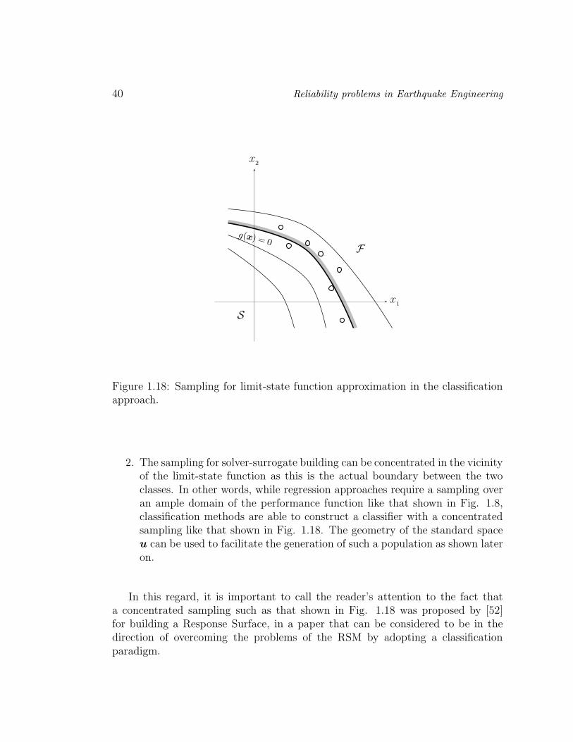
Figure 1.18: Sampling for limit-state function approximation in the classificationapproach.
2. The sampling for solver-surrogate building can be concentrated in the vicinityof the limit-state function as this is the actual boundary between the twoclasses. In other words, while regression approaches require a sampling overan ample domain of the performance function like that shown in Fig. 1.8,classification methods are able to construct a classifier with a concentratedsampling like that shown in Fig. 1.18. The geometry of the standard spaceu can be used to facilitate the generation of such a population as shown lateron.
In this regard, it is important to call the reader’s attention to the fact thata concentrated sampling such as that shown in Fig. 1.18 was proposed by [52]for building a Response Surface, in a paper that can be considered to be in thedirection of overcoming the problems of the RSM by adopting a classificationparadigm.

Basic concepts 41
1.9 FORM and SORM approximations with Sta-
tistical Learning devices
As shown in the preceding, the FORM and SORM approximations to the limit-state function require information on the derivatives of the performance functionat the design point. This information, and especially that required by SORM, isdifficult to obtain in case of implicit limit-state functions. However, this task canbe facilitated by the approximation of the limit-state function with linear flexiblemodels such as RBFN and SVM that implement models (1.49) and (1.51), whichare very similar. Consider for instance the second of them, with the followingparticular choice of the kernel function
K(x, y) = (〈x, y〉 + θ)p (1.54)
where 〈·, ·〉 stands for Euclidean inner product. This is known as the Inhomoge-neous Polynomial Kernel in Pattern Recognition literature [63]. Expanding thisfunction for the particular case of p = 2 yields
K(x, y) =d∑
n=1
d∑
j=1
xnxjynyj + 2θd∑
n=1
xnyn + θ2 (1.55)
The derivative of the estimate with respect to a coordinate xk is, therefore,
∂g(x)
∂xk
=m∑
i
wi∂K(x, xi)
∂xk
=
m∑
i
wi
d∑
n=1n 6=k
xnxknxin
+ 2xkx2ik + 2θxik
(1.56)
In addition,
∂2g(x)
∂x2k
= 2m∑
i
wix2ik
∂2g(x)
∂xk∂xj
=m∑
i
wixkjxij , j 6= k (1.57)

42 Reliability problems in Earthquake Engineering
Similar derivations can be easily carried out for other basis functions. The case ofMulti-Layer Perceptrons is, however, more involved, as is evident upon consideringEq. (1.47), especially if function h(·) applied at the output layer is nonlinear.However, the Jacobian and Hessian matrices can be easily evaluated by numericalprocedures in which use is made of the very network. This is explained at lengthin [55], to which the interested reader is referred.
Methods of analysis
Analytic (Moments) Synthetic (Monte Carlo)
Direct Substitution
Figure 1.19: Methods based on the performance function.
1.10 Methods based on the performance func-
tion
Most methods based on the performance function that have been published thus farare based on the estimation of the density function using moments of the structuralresponse (Fig. 1.19). The moments and/or the density function are obtained eitheron the basis of the principle of maximum entropy ([64]; [65]; [66]), polynomialchaos expansion of the random variables [28], polynomial approximation of thedensities ([67]; [68]; [69]) or kernel density estimation [70]. Also in this groupthere are methods aimed at the direct estimation of the reliability with Eq. (1.4)via Monte Carlo simulation [71], statistical approximation techniques ([72]) orPearson distribution ([73]; see, though, [74]).

Basic concepts 43
The Statistical Learning methods briefly introduced in this chapter (MLP,RBFN, SVM) can also be used for this kind of approach acting as solver-surrogates.To this end they are employed as regression functions for substituting the finite-element code in the calculation of the observed responses that make the perfor-mance functions.

44 Reliability problems in Earthquake Engineering

Chapter 2
Information characteristics of
Monte Carlo simulation
2.1 Introduction
As said in the previous chapter, the basic problem of structural reliability can bedefined as the estimation of the probability mass of a failure domain F defined bya limit state function g(x) of the set of basic random variables x:
Pf =
∫
F
px(x)dx (2.1)
where px(x) is the joint probability density function of the basic variables. Acommon characteristic of the simulation techniques is the aim of reducing thecomputational cost of the Simple Monte Carlo Simulation (SMCS), consisting ingenerating a large population from density px(x), calculating the value of y = g(x)for each sample and, finally, estimating the failure probability as the fraction ofcases for which y = g(x) is less than or equal to zero. According to the classificationregard to structural reliability problem [54], using the results of such repeatedcomputations of the limit state function, the probability of failure can be computedas
45

46 Reliability problems in Earthquake Engineering
Pf =1
N
N∑
i=1
z(xi) (2.2)
where z(x) is the transformation
z(x) =1
2[1 − sgn(y)] (2.3)
of the sign function, defined as
sgn(y) =
−1 if y ≤ 0+1 if y > 0
(2.4)
In practice, a widely used technique for performing Monte Carlo simulation instructural reliability analysis is to stop the simulation when the estimate of thebinomial coefficient of variation of the failure probability, given by [35, 75, 76]:
νb =
√
1 − Pf
NPf
(2.5)
becomes lower than or equal to 0.1. Here N is the actual number of samples forwhich the limit state functions is actually computed. This criterion stems from theassimilation of Monte Carlo simulation to a sequence of Bernoulli trials, so thatthe number of trials reaching the failure domain obey a binomial distribution.
As an illustration, consider the limit state function
g(x1, x2) = 0.1(x1 − x2)2 − 1√
2(x1 + x2) + 2.5
where the random variables x1, x2 are both standard Normal. The probability offailure was computed with 500 populations of N = 25, 000 samples and makinguse of the stopping criterion mentioned above. This was possible in 382 out of the500 cases. Figure 2.1 shows the relationship between the failure probability andthe actual number of samples. The concentration at N = 25, 000 corresponds to128 cases in which the coefficient of variation estimated according to Eq. (2.5)remained higher than 0.1. For the rest of cases, in which it was possible to stopthe simulation at a lower number of the limit state function evaluations, it isevident that, the lower the number of samples, the higher the failure probability.On the other hand, the histogram of the failure probability exhibits a wide rangeof variation, given exactly by [0.0032 0.0060], whereas the mean value computed

Information characteristics of Monte Carlo 47
2.4 2.6 2.8 3 3.2 3.4 3.6
x 104
2
2.5
3
3.5
4
4.5
5x 10
−3
number of samples
prob
abili
ty o
f fai
lure
Figure 2.1: Relationship between the number of samples and the failure probabilitywhen the stopping criterion is applied.
over the 500 populations is 0.0043. Accordingly, the maximum error with respectto this average is 39%, which can be considered very high.
The sample estimate of the coefficient of variation of the failure probability(i.e. the ratio between the standard deviation and the mean) was found to be0.0987. A similar value (0.0936) was obtained without applying the stoppingcriterion supplied by Eq. (2.5), thus indicating that the determining factor for theaccuracy of the failure probability estimation is the number of samples and notthe application of the stopping criterion νb < 0.1. In fact, the above values raiserespectively to 0.157 and 0.150 for N = 10, 000 samples, using also 500 populations.

48 Reliability problems in Earthquake Engineering
On the other hand, notice in Figure 1 that the application of the stopping criterionoccasions the largest departures from the mean value instead of approaching toit, as it could naively be expected. This is due to the dependence of the binomialestimate of the coefficient of variation on the estimate of the probability, accordingto which the larger Pf the lower νb, so that it suffices that the current estimateof the probability be large to stop the simulation. This fact, which has beenobserved in all the analysis reported later in this chapter, clearly indicates thatthe simulation stopping criterion based on the binomial estimate given by Eq.(2.5) can be seriously misleading. According to these observations, the criterion isfound to be more relevant for computational savings than for accuracy benefits.
The use of the basic Monte Carlo method in standard practice of structuralreliability analysis is examined in this chapter, having especially in focus the ran-domness of the estimate (2.2) and the effects of using Eq. (2.5) for stopping thesimulation programme. It is demonstrated that the use of Information Theoryconcepts allows a selection of the population to be used in a Monte Carlo simula-tion in order to obtain a good estimate of the mean value of the failure probability,thus avoiding random estimates which can lie very far from it, and whose sepa-ration from such a mean remains unknown. To be specific, the proposal consistsin generating a large number of populations of the input random variables andselecting that having the average entropy because it leads to an estimate close tothe actual mean value of the probability of failure. Therefore, the entropy providesa preprocessing criterion for selecting the optimal population for the simulation,thus avoiding reliance on νb for yielding the probability estimate and using it onlyfor reducing the number of samples. By means of a theoretical derivation andseveral examples the validity of this proposal is demonstrated.
The next section of the chapter is devoted to a brief exposition of some conceptsof Information Theory which constitute a basis for the proposal presented herein.This is followed by the theoretical and empirical demonstration of the soundnessof the proposal. The chapter ends with some conclusions and directions for futureresearch.
2.2 Some concepts of Information Theory
In this section the essential concepts of Information Theory (IT) that are relevantfor the purposes of the chapter are summarized after [77, 78, 79].
The degree of information offered by a sample regarded as a realization ofa random variable depends on the degree of surprise it provokes in its arising.

Information characteristics of Monte Carlo 49
Thus we can build an information function I(P ) with the simple rule that nonsurprising events, i.e. those having a probability of occurrence P = 1, afford noinformation, while those of little probability are very informative. No, considertwo independent events A and B with probabilities PA and PB. Since the eventsare independent, their joint probability is the product PAB = PAPB. Similarly,the joint information given by the events can be denoted as I(PAPB). In termsof their individual information contents, this joint information can be defined bymean of the following rule:
I(PAPB) − I(PA) = I(PB) (2.6)
This means that the residual information on the joint occurrence of the events, afterreceiving the information that A has occurred, is not different from the informationthat B has occurred, because the events are independent. Presenting the aboveequation as
I(PAPB) = I(PA) + I(PB) (2.7)
indicates that for independent events the joint information is additive, while thejoint probability is multiplicative. From these equations it results that for thesame event
I(P 2) = 2I(P ) (2.8)
and hence
I(P q) = qI(P ) (2.9)
Let r ≡ − ln(P ). Then, P = (1/e)r and applying the previous equation oneobtains
I(P ) = I [(1/e)r] = rI(1/e) = −I(1/e) ln(P ) (2.10)
Defining the scale term I(1/e) ≡ 1, one finally obtains
I(P ) = − ln(P ) (2.11)
This is the so-called self-information of a random event of probability P and itdefines the information content of a certain region of the space. Notice that I(P ) →∞ as P → 0 and I(P ) → 0 as P → 1. In words, the information grows as theevent becomes more rare and diminishes as it becomes more certain, as expected.

50 Reliability problems in Earthquake Engineering
From the above definition of self-information and for the general case of multipleevents, it results that the information content depends on the definition of theregions of the space on which the random occurrences are observed, i.e. on thepartition of the samples space. In practice, for computing the empirical entropyuse is made of the regular partition used for computing histograms. In general, forN samples generated from the distribution function of a vector random variablex, grouped in the bins defined by a partition X = x1, x2, . . ., one can associatethe bin probability estimates Pj = nj/N, j = 1, 2, . . . , n, where nj is the number ofsamples in each bin. The expected value of the information on the variable yieldedby the population is the weighted average of the self-information values:
H(x,X ) = −L∑
j=1
Pj ln Pj (2.12)
where L is the total number of bins. As is well known, this average is calledentropy. For a given population of samples, the corresponding estimate of theentropy is
Hk(x,X ) = −L∑
j=1
nj
Nln
nj
N(2.13)
for k = 1, 2, . . . , M , where M is the number of such populations. For a largenumber of populations M , the estimate of the average entropy is
ˆH(x,X ) =1
M
M∑
k=1
Hk(x,X ) (2.14)
For the ensuing developments it is important to recall two further statements ofInformation Theory. First, that if a partition X ′ is obtained by refining a partitionX , then
H(x,X ) ≤ H(x,X ′) (2.15)
Second, that for a transformation of a discrete random variable x into y = g(x)the following equation holds [79]:
H(y,X ) ≤ H(x,X ) (2.16)
The equality sign holds when the transformation is one-to-one.

Information characteristics of Monte Carlo 51
x1
x2
g(x)=
0
F
S
F
S
x1
x2
g(x)=
0
Figure 2.2: Two realizations of a contrived experiment used for establishing anapproximate relationship between the entropy and the probability of failure.
2.3 Information characterization of Monte Carlo
simulation
According to Eqs. (2.2) to (2.4), each experiment in a Monte Carlo simulationcan be regarded as the transformation of a sample x through a system yielding arealization y of random variable y = g(x) which in turn is transformed by anothersystem yielding the realization z of the random variable z.
In order to examine the relationship between the failure probability and thesample entropy, let us contrive a particular numerical experiment (see Figure 2.2).In it, a global partition is determined by the limit state function and for computingthe empirical entropy (2.13) each domain is partitioned in a certain number of binseach. The populations are generated with the same number of samples. The maincondition of the experiment is that the quantity of the samples in the safe regionS is kept constant. This restriction is justified because the contribution of thesamples in the safe domain to the failure probability estimate given by Eq. (2.1)is null. In contrast, the position of the samples in the failure domain F is allowed

52 Reliability problems in Earthquake Engineering
to vary randomly, so that the empirical entropy given by Eq. (2.13) also becomesrandom, as is evident. Notice that for all the populations k, k = 1, 2, . . . , M ofthis experiment, the estimates of the failure probability Pf,k will be equal to eachother and to the mean computed over all populations thus generated, Pf .
Under such conditions, Eq. (2.12) takes the form
H(x,X ) = −Lf∑
i=1
Pi ln Pi −Ls∑
j=1
Pj ln Pj (2.17)
where Lf is the total number of bins in the failure domain and Ls that of the safedomain. Notice that according to the above exposition the empirical probabilitiesin the failure domain and, accordingly, the empirical entropy, become randomvariables, as indicated by the underlined variables in the preceding equation. Itcan be put in the form
S + H(x,X ) = −Lf∑
i=1
ln PiPi (2.18)
where
S =
Ls∑
j=1
Pj ln Pj (2.19)
is a constant term according to the definition of the experiment. Equation (2.18)can re rewritten as
−Lf∏
i=1
PiPi = exp(S) exp(H(x,X )) (2.20)
Let us now apply the expectation operator to both sides of the preceding equa-tion:
−E
[
Lf∏
i=1
PiPi
]
= E [exp(S) exp(H(x,X ))] (2.21)
For the left-hand side it is evident that
−E
[
Lf∏
i=1
PiPi
]
= −Lf∏
i=1
E[
PP i
i
]
(2.22)

Information characteristics of Monte Carlo 53
because of the independence of Monte Carlo trials. Applying a first order approx-imation, the above product can be estimated as
−Lf∏
i=1
E[
PiPi] .
= −Lf∏
i=1
P Pi
i (2.23)
where Pi is the expected value of the probability in i-th bin of the failure domain.It is evident that it is given by
Pi =Pf
Nf(2.24)
where Nf is the number of samples in the failure domain. Therefore, the right-handside of Eq. (2.21) becomes
−E
[
Lf∏
i=1
PiPi
]
= −[
Pf
Nf
]
(
PfLfNf
)
(2.25)
Noticing that
Pf =Nf
N(2.26)
where N is the total number of samples, Equation (2.25) can be finally put in theform
−E
[
Lf∏
i=1
PiPi
]
= −[
1
N
]
(
PfLfNf
)
(2.27)
On the other hand, for the right-hand side of Eq. (2.21), a first order approxi-mation yields
exp(S)E [exp(H(x,X ))].= exp(S) exp(H(x,X )) (2.28)
where H(x,X ) is the mean entropy. Therefore, reuniting Eqs. (2.27) and (2.28),corresponding to the two sides of Eq. (2.21) and taking logarithms yields
− PfLf
Nfln
1
N= S + H(x,X ) (2.29)
which finally renders the following relationship between the mean entropy and themean probability of failure:

54 Reliability problems in Earthquake Engineering
Pf =Nf
Lf ln N
(
S + H(x,X ))
(2.30)
The meaning of this equation is that there is a linear relationship between themean values of the entropy and the failure probability, for the contrived experimentat least. In the general case, in which the positions and number of the samplesin both domains are allowed to vary in a random fashion, a general relationshipis difficult to establish. However, since the samples in the safe domain, which arethe vast majority, do not contribute at all to the expected value of the failureprobability, the above experiment is close to the actual situation and, therefore,the result given by Eq. (2.30) gives a practical support to the main hypothesis ofthe present chapter, i.e. that the mean failure probability, considered as a randomvariable, can be estimated with a population having a mean entropy among alarge set of candidate ones. Therefore, the failure probability estimate can be
obtained with the population of x having the closest entropy ˆH(x,X ) to thatof the empirical mean of the entropies, computed over all populations using Eq.(2.14):
ˆPf,1 ⇐ ˆH(x,X ) (2.31)
For the sake of completeness, notice that for the simple binary partition B ofthe variable space into two bins, one corresponding to the safe domain and theother to the failure one, the entropy is
H(x,B) = −Pf ln Pf − (1 − Pf) ln(1 − Pf) (2.32)
This function is illustrated in Figure 2.3 for a failure probability fluctuating in thecommon range [1 × 10⁻⁴ 1 × 10⁻³]. Despite this simple theoretical result is oflittle use in practice, because the entropy-based selection of the population woulddirectly depend on the target of the calculation, notice anyhow that it confirmsthe close-to-linear relationship between failure probability and entropy, as in Eq.(2.30) which corresponds to a rather different partition. In fact, making use of Eq.(2.15), H(x,B) < H(x,X ).
In addition, it is important to mention that, due to the randomness of thefailure probability estimate, in the actual practice of Monte Carlo simulation instructural reliability analysis the entire simulation is run several times, normallythree, and the average is delivered as the final result, when the computational
effort thus implied is not severely high. For such cases, besides ˆPf,1, it seems

Information characteristics of Monte Carlo 55
1 2 3 4 5 6 7 8 9 10
x 10−4
1
2
3
4
5
6
7
8x 10
−3
Probability
Ent
ropy
Figure 2.3: Relationship between the entropy of the Bernoulli mass density func-tion and the failure probability.
preferable to deliver the following two additional estimates instead of two randomones obtained by simply repeating the simulation:
1. The failure probability estimate obtained as the average of those correspond-ing to the populations showing the minimum, the average and the maximumentropies, amongst a large set of candidates:
ˆPf,2 =1
3
(
Pf,min + ˆPf,1 + Pf,max
)
(2.33)

56 Reliability problems in Earthquake Engineering
where
Pf,min ⇐ Hmin(x,X )
Pf,max ⇐ Hmax(x,X )
2. The failure probability estimate obtained as the entropy-weighted average ofthose corresponding to the populations showing the minimum, the averageand the maximum entropies:
ˆPf,2 =HminPf,min + ˆH ˆPf,1 + HmaxPf,max
Hmin + ˆH + Hmax
(2.34)
where the arguments of the entropy terms have been omitted for the sake ofclarity.
2.4 Application examples
In this section the application of the proposal of selecting the Monte Carlo popula-tion according to information criteria is illustrated with several benchmark exam-ples taken from [80]. In all cases the variables are standard independent Normal,unless stated otherwise. The number of populations used for all the cases wasM = 500.
1. A convex two-dimensional limit state with a combined term:
g(x) = 0.1(x1 − x2)2 − 1√
2(x1 + x2) + 2.5
This function has been used in the introduction, but it is incorporated hereinfor comparison purposes.
2. A concave two-dimensional function with combined term:
g(x) = −0.5(x1 − x2)2 − 1√
2(x1 + x2) + 3

Information characteristics of Monte Carlo 57
3. A two-dimensional function with a saddle point:
g(x) = 2 − x2 − 0.1x21 + 0.06x3
1
4. A highly convex function:
g(x) = 2.5 − 0.2357(x1 − x2) + 0.00463(x1 + x2 − 20)4
In this case, both variables have mean equal to 10 and standard deviationequal to 3.
5. Another highly concave function:
g(x) = 3 − x2 + (4x1)4
6. A five dimensional parallel system:
g1(x) = 2.677 − x1 − x2
g2(x) = 2.5 − x2 − x3
g3(x) = 2.323 − x3 − x4
g4(x) = 2.25 − x4 − x5
g(x) = max(g1, g2, g3, g4)
7. A three dimensional series system:
g1(x) = −x1 − x2 − x3 + 3√
3
g2(x) = 3 − x3
g(x) = min(g1, g2)
8. A three dimensional parallel system:
g1(x) = −x1 − x2 − x3 + 3√
3
g2(x) = 3 − x3
g(x) = max(g1, g2)
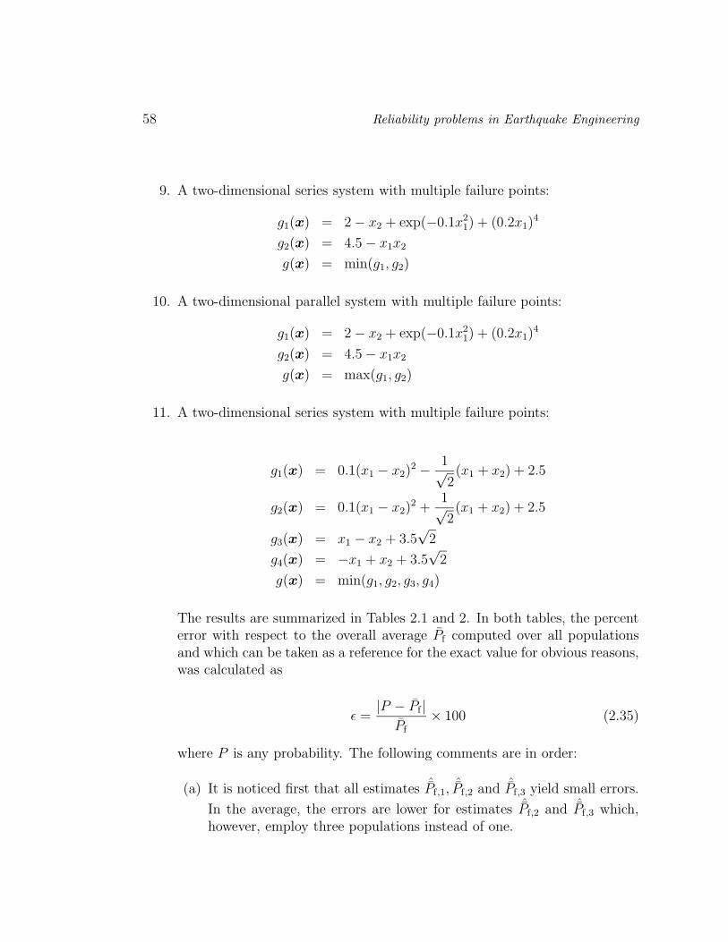
58 Reliability problems in Earthquake Engineering
9. A two-dimensional series system with multiple failure points:
g1(x) = 2 − x2 + exp(−0.1x21) + (0.2x1)
4
g2(x) = 4.5 − x1x2
g(x) = min(g1, g2)
10. A two-dimensional parallel system with multiple failure points:
g1(x) = 2 − x2 + exp(−0.1x21) + (0.2x1)
4
g2(x) = 4.5 − x1x2
g(x) = max(g1, g2)
11. A two-dimensional series system with multiple failure points:
g1(x) = 0.1(x1 − x2)2 − 1√
2(x1 + x2) + 2.5
g2(x) = 0.1(x1 − x2)2 +
1√2(x1 + x2) + 2.5
g3(x) = x1 − x2 + 3.5√
2
g4(x) = −x1 + x2 + 3.5√
2
g(x) = min(g1, g2, g3, g4)
The results are summarized in Tables 2.1 and 2. In both tables, the percenterror with respect to the overall average Pf computed over all populationsand which can be taken as a reference for the exact value for obvious reasons,was calculated as
ǫ =|P − Pf |
Pf
× 100 (2.35)
where P is any probability. The following comments are in order:
(a) It is noticed first that all estimates ˆPf,1,ˆPf,2 and ˆPf,3 yield small errors.
In the average, the errors are lower for estimates ˆPf,2 and ˆPf,3 which,however, employ three populations instead of one.

Information characteristics of Monte Carlo 59
Table 2.1: Entropy-based estimates
No. N PfˆPf,1 ǫ ˆPf,2 ǫ ˆPf,3 ǫ
(%) (%) (%)1 25,000 0.00429 0.00476 11.1 0.00433 1.04 0.00433 1.042 1,000 0.106 0.103 2.5 0.106 0.0 0.106 0.03 3,000 0.0352 0.0394 11.8 0.0339 3.8 0.0339 3.84 35,000 0.00290 0.00288 0.9 0.00282 2.8 0.00283 2.85 600,000 0.000181 0.000169 6.8 0.000171 5.3 0.000171 5.36 500,000 0.000215 0.000211 2.0 0.000205 4.4 0.000206 4.47 40,000 0.00260 0.00250 3.9 0.00261 0.5 0.00261 0.58 850,000 0.000126 0.000113 10.0 0.000128 1.8 0.000128 1.89 30,000 0.00352 0.00371 5.4 0.00367 4.4 0.00367 4.410 400,000 0.000244 0.000223 8.9 0.000228 6.4 0.000228 6.411 50,000 0.00225 0.00245 9.1 0.00234 4.2 0.00235 4.2
Table 2.2: Ranges of fluctuation of probability estimates
No. min Pf ǫ N max Pf ǫ N(%) (%)
1 0.00316 26.2 25,000 0.00596 39.0 16,6762 0.077 27.0 1,000 0.149 40.9 5783 0.0254 27.7 3,000 0.0489 40.0 1,9624 0.00204 29.9 35,000 0.00403 38.9 24,7895 0.000137 24.5 600,000 0.000261 44.5 38,2436 0.000155 27.9 500,000 0.000299 39.3 333,8377 0.00197 23.9 40,000 0.00361 38.8 27,7058 0.000093 25.8 850,000 0.000169 34.0 592,7039 0.00263 25.0 30,000 0.00474 34.9 21,17510 0.000183 25.1 400,000 0.000336 37.8 297,22511 0.00151 33.0 50,000 0.00323 43.8 30,927

60 Reliability problems in Earthquake Engineering
(b) Secondly, it can be seen that the errors associated to the minimum andmaximum probabilities are much larger than those corresponding tothe entropy-based selected populations. The magnitude of this errorsindicates that the application of simple Monte Carlo simulation withouta selection preprocess may occasion to incur in errors up to 40%.
(c) Third, it is noticed that the errors corresponding to the maximum prob-ability are systematically higher than those of the minimum probability.This is due to the fact that, in applying the stopping criterion basedon the binomial estimate of the failure probability νb, it suffices thatthe probability being currently estimated by the simulation be large(i.e. that the number of samples found in the failure domain be large)for the simulation to stop when a νb < 0.1 is reached. In fact, thenumber of samples actually used for computing the maximum proba-bility was smaller than the scheduled number of samples, which for allthe cases was required by 30% of the populations in the average. Thisresult demonstrates the inadequacy of νb < 0.1 as the simulation stop-ping criterion in terms of accuracy, and that it is a good method forcomputational savings only.
Chapter 3
Seismic random variables
3.1 Introduction
In a paper reviewing the criticism addressed to standard methods of seismic designpractice and contemporary proposals for their improvement [81], the authors pro-pose several strategies for obtaining safer designs, one of which is the probabilisticanalysis of the structural system, in recognition of the large uncertainties posedby the seismic action. In fact, while the coefficient of variation (COV) of ran-dom variables present in the design for gravity loads are normally lower than 0.25,variables such as the peak ground acceleration for a return period of 475 years,which determines the entire design according to current practices, is estimated tohave a COV in the range from 0.56 to 1.38, according to the same authors. Inaddition, there is the randomness associated to the seismic acceleration historyas such, which have been modeled as a realization of a random process of even arandom field, implying thousands of random variables in an adequate modeling.
A serious criticism that may be addressed to standard seismic design practiceis that probabilistic considerations in design codes are normally limited to thedefinition of the probability of exceeding a critical value by the peak ground accel-eration in the estimated life of the structure, while no probabilistic verifications ofthe structural responses are required. Since evidently design codes condition thedesign software and even the average amount of knowledge commonly regarded assufficient for design practice, the paradoxical result is that probabilistic concepts
61

62 Reliability problems in Earthquake Engineering
and methods find little application in the field of structural engineering in whichthe uncertainties are the largest.
It may be objected that a full and accurate probabilistic analysis implies largecomputational efforts posed by the general technique known as Monte Carlo simu-lation. To this objection it may be replied that the same criticism has rarely, if atall, been addressed to a deterministic technique requiring huge hardware capabili-ties, which is the Finite Element method, and, on the contrary, its users routinelydemand increasing amounts of computer resources and significant research is de-voted to the subject of parallelization.
Such a bias in this regard to computer technology exploitation betrays a prob-lem of engineering education [82]. In fact, engineering emerged from the paradigmof exactness and accuracy, a label assumed by physics and other sciences, whichhas its roots in the mathematical interpretation of nature. With such an origin,engineering education favors the deterministic regard over the probabilistic one be-cause the randomness arising in natural phenomena is regarded simplistically as adeficiency in the mathematical model, a drawback that is expected to be remediedin the near or distant future. Meanwhile, current deterministic models for dealingwith random environments are used with caution. These naive thoughts are be-hind the well-known safety factors, which hardly relate to elementary probabilisticmeasures of safety, according to a recent research [83]. While a satisfactory deter-ministic model is perhaps possible in some simple cases, in others such an ideal islargely impractical or even impossible. This is specifically the case of Seismologyand Earthquake Engineering, for obvious reasons. This renders illusory the ideal ofa complete deterministic earthquake-resistant design and sheds light on the needof developing practical methods for incorporating probabilistic computation in thedesign practice in order to have adequate measures of the risk involved in eachdesign, thus making better use of computer technology in seismic design.
This chapter is intended to contribute to such desirable goals. Two main prob-abilistic design approaches, namely the Robust Design Optimization (RDO) andthe Reliability-based Design Optimization (RBDO), are focused. While the for-mer operates on estimates of first- and second-order statistical moments of thestructural responses, in the latter decisions are based on probabilities of exceed-ing critical response thresholds (probabilities of failure). The chapter is organizedas follows. First, after a brief exposition of RDO and RBDO, some well estab-lished stochastic models of the seismic action are exposed. The fundamentals ofrandom vibration analysis of linear and nonlinear structures, which yields satisfac-tory estimates of the low order moments, is next summarized. Then the problemof an accurate computation of the structural robustness for earthquake demands

Seismic random variables 63
is addressed. It is shown that the combination of analytical random vibrationtechniques with the method of Point Estimates is sufficient for practical robustdesign. The important problem of a practical computation of the probabilitiesof failure for seismic actions is finally addressed. This is a case in which analyt-ical methods of random vibration are far from satisfactory and resort has to bemade to the synthetic approach, i.e. Monte Carlo simulation. In order to reducethe large computational effort implied by a full Monte Carlo calculation, a mixedanalytic-synthetic approach is proposed. It consists in a treatment of a small setof responses computed by both techniques using the Total Probability Theorem(TPT) and a new sampling method named Backward Stratified Sampling (BSS.By means of an example concerning a base isolated building, it is shown that themethod offers an economical as well as elegant solution to this important step ofreliability-based seismic design.
Considering the specialization of the field of stochastic dynamics and, at thesame time, the practical orientation of present book, the chapter is as self-containedas possible.
3.2 Robust and Reliability-based design options
Proposals for the consideration of uncertainties in seismic design can be groupedinto two main categories: (a) Robust Design Optimization (RDO), which is ori-ented to minimizing the structural cost as well as the spread of the structuralresponses, as measured by low-order statistical moments [84, 85]; (b) Reliability-Based Design Optimization (RBDO), which minimizes the cost function with prob-abilistic constraints [86, 87, 88, 89].
A common formulation of RBDO can be formally presented as follows:
Reliability − based optimization :
find : y
minimizing : C(y) (3.1)
subject to : P[fi(x, y) > Fi] ≤ Qi, i = 1, 2, . . .
y− ≤ y ≤ y+
where C(y) is the cost function depending on the design variables collected invector y, x is a set of random variables, P[A] the probability of the random eventA and Q
iits limiting value. Function gi(x, y) = Fi − fi(x, y) is the function

64 Reliability problems in Earthquake Engineering
known in structural reliability as the limit state function. On the other handy− and y+ are bounds imposed to the design variables, normally constitutinggeometric constraints. For seismic design it has been suggested that the targetprobabilities correspond to a reliability index β = 1.75, so that Qi = 0.0401 [90].
Some researchers and designers, however, favor the design guided by the con-cept of robustness, understood as safety against unpredictable variations of thedesign parameters. Mathematically speaking, robustness can be defined in severalforms, depending on whether use is made of the clustering [91] or conventional,frequentist interpretation of uncertainty. In this chapter the second interpretationis adopted. A possible formulation of this task is
Robust optimization :
find : y
minimizing : C(y) (3.2)
subject to : fi (µz(x, y), σz(x, y)) ≤ 0, i = 1, 2, . . .
y− ≤ y ≤ y+
where µz(x, y), σz(x, y) are respectively the mean and standard deviation vectorsof structural responses collected in vector z, and fi(·, ·) are functions thereof.
The nature of these two alternative methods can be explained with the help ofFig. 1, which shows two alternative probability density functions of a structuralresponse. While RDO aims to reduce the spread, RBDO is intended to bound theprobability of surpassing the critical threshold. Notice that in applying RDO theeffect pursued by RBDO is indirectly obtained, because the reduction of the spreadimplies a reduction of the failure probability. The reliability (or its complement,the failure probability) refers to the occurrence of extreme events, whereas therobustness refers to the spread of the structural responses under large variationof the input parameters. This is assumed to assure a narrow response densityfunction, which in turn assures a low failure probability, if it is unimodal, as iscommon case. However, this is not necessarily true: to a significant spread of thestructural response may correspond a low failure probability because the definitionof the limit state can be such that the possibility of surpassing it is very rare, asthe situation it describes is rather extreme (See Fig. 1).
In this chapter no discussion is made on whether the robust or the reliabilityapproaches is more suitable for the specific problem of seismic design under un-certainties; nor a specific numerical method for solving either RDO nor RDBO isproposed, for which the reader is referred to specialized references [84, 92, 93, 94,

Seismic random variables 65
z
pz(z)
Figure 3.1: Robust and reliability-based design options. While the first aims atreducing the spread of the response function, the second attempts to control theprobability of surpassing a critical threshold (dashed line). However, low failureprobabilities may correspond to large spreads (dotted line).
95, 96, 97, 85]. Instead, the chapter is oriented to propose practical techniquesfor calculating the stochastic quantities implicit in these methods, namely low or-der response moments and failure probabilities under earthquake ground motionexcitations.
3.3 Stochastic models of seismic action
In this section some useful equations for a stochastic modeling of the seismic actionin design practice are recalled. First, convenient way of modeling the groundmotion acceleration is the response of one or more linear filters excited by a whitenoise. Two models have found extensive application in practice, namely the Kanai-

66 Reliability problems in Earthquake Engineering
ω
G(ω)
ωgωf
Figure 3.2: Clough-Penzien seismic spectral model.
Tajimi and the Clough-Penzien filters. In the former case, a linear system is
ug + 2 νgωgug + ω2gug = −w(t) (3.3)
where w(t) is a white noise. The other parameters appearing in this equation havealready been explained. In the latter case, it is necessary to append, in addition,the equation
uf + 2 νfωf uf + ω2f uf = −
(
2 νgωgug + ω2gug
)
(3.4)
meaning that the Clough-Penzien filter is driven by a compound excitation givenby the sum of the velocity and displacement responses of the Kanai-Tajimi filter.The Clough-Penzien better represents the actual power spectrum of earthquakes,

Seismic random variables 67
as this features a decreasing energy as ω → 0. For the Clough-Penzien model thepower spectrum is given by [98]
G(ω) =ω4
g + 4ν2gω
2gω
2
(ω2g − ω2)2 + 4ν2
gω2gω
2· ω4
(ω2f − ω2)2 + 4ν2
f ω2f ω
2G0 (3.5)
where ωg and νg are parameters associated to the dominant soil frequency anddamping, respectively, ωf and νf give the spectrum a necessary decreasing shapein the low frequency region, and G0 is the constant power spectral density of theunderlying white noise w(t). The Clough-Penzien spectral density is shown in Fig.3.2.
In practice, the intensity of the white noise can be related to the peak groundacceleration Ag by [99, 100]
G0 = 2
(
Ag
28.4
)2
(3.6)
On the basis of random vibration theory it is possible to derive other analyticalequations for estimating response quantities of linear and, in some case, nonlinearsystems [101, 102, 103]. For instance, a useful equation for estimating the spectraldisplacement of a linear SDOF system is [104]
Sd(ω, ν) = λ(s, R) σu (3.7)
where σu is the standard deviation of the displacement response and λ(s, R) theso-called peak factor, which is a function of the duration of the motion in itsstationary phase s0 and R the probability of the system to remain below the levelSd(ω, ν). In other words, R is the reliability that the designer intends to conferto the system and thus it is given by R = 1 − Q, where Q is the limiting failureprobability in the optimization (see Eq. 3.1). The standard deviation of thedisplacement can be obtained from the following expression:
σ2u =
1
ω4
ωG(ω)
(
π
4νs− 1
)
+
ω∫
0
G(Ω)dΩ
(3.8)
On the other hand, the peak factor is approximately given by
λ(s, R) ≈
√
√
√
√2ln
(
− ωs
πlnR
[
1 − exp
−√
4νsln(
− ωs
πlnR
)
])
(3.9)

68 Reliability problems in Earthquake Engineering
where
νs =ν
1 − exp(−2νωs0)(3.10)
where s0 is the duration of the strong motion phase. A useful regression equationfor this parameter is [105, 106]:
s0 = 30 exp(
−3.254 A0.35g
)
(3.11)
Sample
ms(t
)
m−
1s(t
)...
3s(t
)
2s(t
)
1s(t
)
t
s(t)
t 21s(t2
)2s(t2
)
3s(t2
)m−
1s(t2
)ms(t2
)
t 11s(t1
)2s(t1
)3s(t1
)m−
1s(t1
)ms(t1
)
Figure 3.3: Realizations of a random process.
On the basis of the power spectral density function it is possible to generateartificial accelerograms. A first step is the generation of realizations of the sta-tionary random process, such as those shown in Fig. 3.3. To this end a practicalalgorithm is [107]:
s(t) =
J∑
j=1
√
2G(ωj)∆ω cos(ω
jt + ζ
j) (3.12)
where J is a large number (of the order of one or two thousands), ζj
is a randomnumber having uniform distribution in the range [0, 2π], ∆ω is the resulting interval

Seismic random variables 69
in the discretization of the ω−axis into J frequencies. This equation indicates thatthe signals s(t) are the result of a large sum of harmonics with random phaseshaving an amplitude depending on their value in the power spectrum. In orderto obtain a realistic accelerogram it is necessary to give a non-stationary shape tothe signal. This is achieved using
ug(t) = ξ(t)s(t) (3.13)
where ξ(t) is a function characterized by three phases: an ascendent one, corre-sponding to the first trains of seismic waves, a flat one associated to the strongground motion and a descending one. There are several proposals for this function.Among them, the Amin-Ang modulating function [108] fits well in the modelingof the seismic action dealt with in this chapter, as it can be made dependent onthe duration of the strong motion phase, given by Eq. (3.11). It is given by
ξ(t) =
(
tt1
)2
if t ≤ t1
1 if t1 ≤ t ≤ t2exp (−c(t − t
2)) if t2 < t
(3.14)
with parameters t1
corresponding to the start of the strong motion phase, t2
=t1+ s0 and c, a parameter used for modeling the waning phase of the acceleration
history.For the purposes of present chapter it is important to remark that all pa-
rameters referred hereto are highly random. This means that in addition to therandomness of the acceleration history as such, the uncertainty about the underly-ing stochastic model must be considered for an adequate computation of structuralrobustness and reliability. Among the parameters defining the model, those havingthe largest impact into the uncertainty spread are
x = ωg, νg, Ag (3.15)
The peak ground acceleration, normally defined as that having a 10% probabilityof being exceeded in 50 years, can be modeled as a Lognormal variable with acoefficient of variation equal to 0.6, according to the research reported in [109] (Themean value of Ag depends on the seismicity of the region under consideration). Itmust be noted, however, that the randomness of the peak ground accelerationmay be larger, since according to a study quoted in [81] its coefficient of variationlies in the range from 0.56 to 1.38. For the other two parameters the statisticalanalyses reported in [105, 106] yield the values appearing in Table 3.1. Note that

70 Reliability problems in Earthquake Engineering
the uncertainty of all these variables is very large. According to the informationgiven in [106], the correlation among all these variables is close to zero, so that thecovariance matrix can be taken as diagonal. In addition, there are two dependentrandom variables, namely the strong motion duration and the white noise powerspectral intensity, given respectively by Eqs. (3.11) and (3.6).
Table 3.1: Probabilistic definition of spectral random variables
Parameter Distribution Mean c.o.v.ωg Gamma 20.3 rad/s 0.448νg Lognormal 0.32 0.421Ag Lognormal — 0.6
For the ensuing analyses with this modeling, the rest of parameters are assumedwith the following fixed values: t
1= 2s, c = 0.18, ωf = 2rad/s and νf = 0.6.
3.4 Fundamentals of random vibration analysis
As is well known, the dynamics of a linear structure with mass, viscous dampingand stiffness matrices denoted by M , C and K, respectively, is given by [98]
Mu(t) + Cu(t) + Ku(t) = p(t) (3.16)
where u, u and u are the displacement, velocity and acceleration vectors, respec-tively. With the aim of calculating the statistical second order response of thestructure, it is convenient to express the above system of equations in state spaceform. That is, by collecting the displacement and velocity responses in the statevector qT(t) = [uT(t), uT(t)], the original system of l second order differentialequations is transformed into the following system of 2l first order differentialequations:
q(t) = Aq(t) + f (t) (3.17)
Here A is the so-called system matrix given by
A =
(
0 I
−M−1K −M−1C
)
(3.18)

Seismic random variables 71
and the vector of external loads is then
f (t) =
(
0
−M−1p(t)
)
(3.19)
Let us now derive the differential equations governing the evolution of thefirst and second order moments of the random response of a linear structure,when excited by an external load defined as a stochastic process p(t). Under thisstochastic point of view Eq. (3.17) is written as
q(t) = Aq(t) + f(t) (3.20)
The application of the expected value operator E[·] to this equation gives theevolution of the vector of mean responses
µ(t) = Aµ(t) + µf (t) (3.21)
For the sake of simplicity in the derivation of the covariance evolution, let usassume that the excitation and, consequently, the response have zero mean. Thecovariance matrix is defined as
Σ(t) = E[q(t)q(t)T ] (3.22)
For instance, in the case of a SDOF system, its entries are
Σ(t) =
(
σ2u(t) σuu(t)
σuu(t) σ2u(t)
)
(3.23)
where σu(t), σu(t) are the standard deviations of the displacement and velocity,respectively, and σuu(t) their covariance. The time derivative of the covariancematrix is given by
Σ(t) =d
dtE[q(t)qT(t)] (3.24)
with the result
Σ(t) = E[Aq(t) + f(t)qT(t)] + E[q(t)Aq(t) + f(t)T ] (3.25)
which leads to

72 Reliability problems in Earthquake Engineering
Σ(t) = AE[q(t)qT(t)] + E[q(t)qT(t)]AT + E[f (t)qT(t) + q(t)fT(t)] (3.26)
that is,
Σ(t) = AΣ(t) + Σ(t)AT + E[f (t)qT(t) + q(t)fT(t)] (3.27)
For seismic ground motions, the system of equations of motion (Eq.3.16) mustbe enlarged to include the filter equations (3.3) and (3.4). Accordingly, the vectorof external forces in Eq. 3.16 excited by the filter acceleration uf takes the form
p(t) = −Mrξ(t)uf(t) (3.28)
where r is a vector of static structural displacements caused by a unit static groundmotion [98]. Thus, the leading underlying excitation is a single white noise (seeEq. 3.3). It can be shown that under such an excitation the last term of the aboveequation becomes
E[f (t)qT(t) + q(t)fT(t)] = π
(
0 0
0 b
)
(3.29)
with
b = M−1rrTM−1ξ2(t)G0 (3.30)
The differential equation for the evolution of the covariance matrix finally becomes
Σ(t) = AΣ(t) + Σ(t)AT + πSf (t) (3.31)
where
Sf (t) = π
(
0 0
0 b
)
(3.32)
For nonlinear structures, the method of equivalent linearization [110, 111, 112]is perhaps the only non-Monte Carlo approach that can be readily applied tolarge systems [113]. For the common case displacement and velocity dependentnonlinear restoring forces,
Mu(t) + Cu(t) + H(u, u)(t) = p(t) (3.33)

Seismic random variables 73
t
σu
Figure 3.4: Comparison of Gaussian (dashed line) and non-Gaussian stochasticequivalent linearization (solid line) for an hysteretic oscillator using Monte Carloresults (dotted line)
the method consists in first finding equivalent matrices Ce and Ke for building asystem of equations of the form
Mu(t) + Ceu(t) + Keu(t) = p(t) (3.34)
and then applying the above procedures for finding the covariance evolution. Theequivalent matrices are found through the minimization of the expected value ofthe squared difference between Eqs. (3.33) and (3.34). As a result, the entries ofthese matrices become dependent on the covariance responses at each time step,i.e. they are time-varying. If it is assumed that the responses are Gaussian thecomputations for some hysteretic systems, such as the Bouc-Wen model [114] aregreatly facilitated [115]. Despite this assumption yields satisfactory results for sta-tionary analysis (in which Σ(t) = 0) [110], the results may be far from satisfactoryfor the nonstationary case [116]. For this reason other, non-Gaussian approacheshave been proposed [36, 117, 116]. As an illustration, Fig. 3.4 shows the results

74 Reliability problems in Earthquake Engineering
for the standard deviation of the displacement of a Bouc-Wen hysteretic systemdriven Clough-Penzien seismic excitation, calculated with Monte Carlo simulation,equivalent linearization with Gaussian assumption and the non-Gaussian methodof reference [116].
3.5 Practical computation of seismic robustness
In this section the problem of computing measures of the structural robustnessunder the input of earthquake loads is addressed. As said in the preceding, suchmeasures are the statistical response moments of the first two orders. Exceptin cases of severe nonlinear behavior (such as the liquefaction of soils), it canbe assumed that the responses to earthquakes have zero mean. Accordingly, forresponses such as displacements, velocities and restoring forces it is sufficient tosolve the equation of the evolution of the covariance matrix (3.31). However, ifrobustness is specified in terms of maximum responses in the absolute sense, themean value will be different from zero. To this end the following procedure yieldsgood estimations [118].
3.5.1 Moments of maximum response
Let zm denote the maximum of a random variable z. In [118] it is postulated thefollowing Gumbel-type distribution function for a maximum occurring betweentime instants t1 and t2 :
F (zm, t1, t2) = exp[
− exp
−Kη−1(zm
ǫ− K
)]
(3.35)
where the parameters η and ǫ depend on the time instants t1 and t2 and the firsttwo moments of the peaks occurring in that interval. The latter are given by
µP(t1, t2) =
√π
2
1
t2 − t1
∫ t2
t1
σz(t)dt (3.36)
σ2P(t1, t2) =
2
t2 − t1
∫ t2
t1
σ2z(t)dt (3.37)
where σz(t) is the standard deviation of z. On the other hand, η and ǫ can beobtained by solving the following system of nonlinear equations:

Seismic random variables 75
0 1 2 30
1
2
3
T
σ
Figure 3.5: On the accuracy of the Point Estimate technique for calculating thespectrum of the unconditional standard deviation of SDOF displacement. Solidline: Point Estimate method. Dashed line: Monte Carlo simulation (1,000 sam-ples). The dotted line corresponds to the standard deviation without consideringuncertainties in the Kanai-Tajimi model and using the mean values of the param-eters.
σP(t1, t2)
µP(t1, t2)=
[
Γ(
2η
+ 1)
− Γ2(
1η
+ 1)]
1
2
Γ(
1η
+ 1) (3.38)
µP(t1, t2) = ǫη1
η Γ
(
1
η+ 1
)
(3.39)

76 Reliability problems in Earthquake Engineering
where Γ(·) is the Gamma function. The value of K is expressed in terms of thetime-varying zero upcrossing rate of the process λ↑(t), i.e. the mean rate at whichthe process crosses the time axis with positive slope:
K =
[
η ln
∫ t2
t1
2λ↑(t)dt
]1
η
(3.40)
It has been reported that the use of the zero upcrossing rate of Gaussian processesgives satisfactory results. This is given by
λ↑(t) =σz(t)
√
1 − ρ2zz(t)
2πσz(t)(3.41)
where σz(t) is the standard deviation of the time derivative of z and ρzz =σzz/(σzσz) the correlation coefficient of z and z, as given by the second orderanalysis (3.31). Note that since the postulated distribution of the maximum is ofthe Gumbel type, the mean and standard deviation of the maximum are
µzm(t) = (K + 0.577K1−η)ǫ (3.42)
σzm(t) =
πǫ√6K1−η
(3.43)
3.5.2 Unconditional moments
In order to assure the robustness of the structural system under the action ofearthquake loads it is not sufficient to use a stochastic model of the ground motionexposed in the preceding. This is due to the fact that some of the parametersdefining the model are highly random. Therefore, a correct estimations of thestatistical moments of the response requires the consideration of such a randomnessin a satisfactory manner. In this paragraph the main methods for accomplishingthis task are discussed, with special emphasis on the Point Estimate technique,which to this purpose has been found accurate and simple to apply.
Perturbation methods, based on the Taylor expansion of the response vector q,have been proposed to the purpose of computing the sensitivity of the statisticalmoments to variations of the random variables x [100, 119, 120]. Considering q afunction of the vector of parameters x, the first order expansion for the covarianceresponse yields

Seismic random variables 77
0 1 2 30
5
10
15
20
25
T
Increment (%)
Figure 3.6: Spectrum of the increment of the standard deviation of the SDOFdisplacement when considering the uncertainties of the Kanai-Tajimi model pa-rameters.
∂Σ(t)
∂x=
∂A(t)
∂xΣ(t) + A(t)
∂Σ(t)
∂x+
∂Σ(t)
∂xAT (t) + Σ(t)
∂AT (t)
∂x+ π
∂Sf (t)
∂x(3.44)
The matrix ∂Σ(t)/∂x contains the sensitivities of the second order responseswith respect to the seismic parameters. With these sensitivities the increase ofthe statistical moments due to the parameters’ spread can be estimated. How-ever, perturbation methods in general are accurate only for parameters having acoefficient of variation of, say, less than 0.1. Since all the seismic parameters con-sidered herein have a much larger spread, this technique should be discarded forthis application.

78 Reliability problems in Earthquake Engineering
Let us consider now the application of Monte Carlo simulation, consisting insolving repeatedly Eq. (3.31) using a random realization of vector x in eachanalysis and then computing the average of the variances and covariances of thestructural responses. To this end the use of techniques oriented to estimate loworder statistical moments of the responses with a small number of samples, suchas the Latin Hypercube sampling [2], is recommended. However, as shown next,the method of Point Estimates is perhaps the most practical solution.
The method of Point Estimates was originally proposed in [121] and has beenapplied in several areas of structural engineering research, including EarthquakeEngineering [122, 123, 124]. Its main difference with respect to the perturbationapproach is that it is intended to cancel the higher order terms in the Taylorexpansion instead of disregarding them. There are several proposals for applyingthis concept [121, 125, 126, 127, 128]. The simplest variant of those proposed in[128] will be evaluated for its application in the seismic design context.
For uncorrelated parameters, which is the case considered herein, the methodpostulates a linear equation for the moments of the system response h(x), regardedas a function of a random parameter x, in the form
E[hj(x)] =n∑
k=1
m∑
i=1
wk,ih(xk,i)j j = 1, 2, . . . (3.45)
in which n is the number of variables and m is the number of concentration points.The function h(·) is evaluated at points xk,i = µx + ξk,iσx, i = 1, 2, where µx andσx are respectively the mean and standard deviation of the random parameters.For each variable k the values of the weights wi and the normalized evaluationcoordinates ξi are [128]
ξi =γ3
2+ (−1)3−i
√
n+(γ3
2
)2
wi =1
n(−1)i ξ3−i
ζ(3.46)
with ζ = 2√
n + γ23/4. Here γl is a normalized central moment defined as
γl =1
σl
∫ ∞
−∞(x − µ)lp(x)dx (3.47)
where p(x), µ and σ are respectively the probability density function, the meanand the standard deviation of the variable x.

Seismic random variables 79
In order to evaluate the accuracy of this method, it has been applied to theestimation of the spectrum of the unconditional standard deviation of the dis-placement of a SDOF linear system with damping ratio ξ = 0.05. To this enduse is made of the Total Probability Theorem, applied to estimate the uncondi-tional variance of the structural displacement u(x), considered as a function of theground motion parameters x = ωg, νg, Ag, as follows:
Var(u) =
∫
Var(u(x)|x)px(x)dx (3.48)
where Var(u(x)|x) is obtained by means of the theory of random vibration as [98]
Var(u(x)|x) =
∫
1
(ω2 − Ω2)2 + 4ξ2Ω2ω2· G(Ω, x)dΩ (3.49)
where G(Ω, x) is the power spectral density of the Kanai-Tajimi seismic model:
G(Ω, x) =ω4
g + 4ν2gω
2gΩ
2
(ω2g − Ω2)2 + 4ν2
gω2gΩ
2G0 (3.50)
Taking into account that the mean of the random displacement is zero, theunconditional variance of the response, given by Eq. (3.48), is estimated with thepoint estimate technique as
Var(u) =n∑
k=1
m∑
i=1
wk,iVar (u(xk,i)) (3.51)
using the probabilistic definition of the parameters x displayed in Table 3.1. Forthe parameter Ag a mean value equal to 0.25g has been employed. The concen-tration points and weights are as shown in Table 3.2.
Table 3.2: Values for the application of the Point Estimate method with stochasticKanai-Tajimi spectrum
Parameter x1 w1 x2 w2
ωg 8.1852 0.2079 40.2275 0.1254νg 0.1601 0.2266 0.6596 0.1067Ag 0.1006 g 0.2505 0.7018 g 0.0828

80 Reliability problems in Earthquake Engineering
The results are shown in Fig. 3.5. Notice that with only six calculations of theSDOF system per period, the results are in excellent agreement with the estima-tion yielded by Monte Carlo simulation obtained as the average of 1,000 calls of Eq.(3.49) for each period. The figure also displays the spectrum of the standard de-viation without considering the uncertainties of the model parameters. The effectof such a consideration can be better appreciated in Fig. 3.6, which correspondsto the increment of the standard deviation using the uncertain stochastic modelwith respect to its use with mean values. It can be observed that the impact of theuncertainties is more important at lower periods than at larger ones, for which theincrement stabilizes at about 17%. This result points out the relevance of usinga full stochastic model for structural robustness computations under earthquakeloads.
The above discussion suggests that the Point Estimate method in the versionreported in [128] constitutes an excellent means to evaluate the unconditionalstructural robustness in Earthquake Engineering.

Chapter 4
Practical computation of seismic
reliability
4.1 Introduction
A distinguishing feature of probabilistic mechanics is the availability of an en-tirely general and accurate method for evaluation of statistical characteristics ofthe structural responses, such as moments, distribution functions and probabili-ties, which is the Monte Carlo method. In fact, the method can be regarded asa sampling technique in the probability space yielding a large population of thestructural responses. In its turn, this population can be regarded as the secondbest piece of information after the explicit knowledge of their joint probabilitydistribution, which is normally unknown. On the other hand, the Monte Carlomethod is general in the sense that it is not limited by the mechanical character-istics of the system under analysis, such as linearity or any kind of nonlinearity.However, as is well known, its basic restriction is that the number of samples nec-essary to yield meaningful results is large and, in some cases, prohibitively large.For this reason resort is commonly made to other, non-general and approximatemethods based on simplifying assumptions, whose computational cost, however, ismuch lower.
In this chapter two practical procedures for the reliability assessment under
81

82 Reliability problems in Earthquake Engineering
seismic loads are proposed. The first is a Monte Carlo technique consisting in ap-plying a backward sampling procedure using an algorithm based on the Dealunaytessellation intended to reduced the number of solving calls. due to computationalreasons the algorithm is restricted to cases with a reduced number of variables,which is just the case of the seismic problem when use is made of random vibrationapproaches, as explained in Chapter 2, since in this case the problem is dominatedby the set of variables x = ωg, νg, Ag. The second is a method for improvingthe accuracy of the estimates of the probability of failure given by such simplifiedprobabilistic methods. It is based on the Total Probability Theorem applied toa small sample computed in parallel with both the simplified method and MonteCarlo simulations. The method is applied in connection with a sampling tech-nique introduced herein, named Backward Stratified Sampling, intended to causea further reduction of the number of deterministic solver calls.
4.2 Backward Sampling with Delaunay tessella-
tion
In this section a practical procedure for computing the failure probability whenusing Monte Carlo simulation. For computational reasons it is restricted to thecase of a reduced number of random variables.
Consider a Monte Carlo sample in u−space that has been selected accordingto the entropy criterion exposed in Chapter 2. Taking into account that only afew samples lie in the failure region, an obvious method for reducing the numberof structural solver calls is to avoid using the solver with samples lying in the saferegion. To this end it is advisable to sort the samples according to the distanceto the origin in the u−space and to remove those lying inside a hyper-sphere ofradius β, which corresponds to a rough estimate of the reliability index of theproblem at hand. This is illustrated by figure 4.1 which corresponds to the limitstate function
g(x) = 2 − x2 − 0.1x21 + 0.06x3
1
used in the discussions of Chapter 2. It can be seen that by this means an impor-tant reduction in the number of samples in comparison to the crude Monte Carlomethod is achievable. However, a further reduction is possible by means of theDelaunay tessellation, which is defined as follows: given a set of data points, itis a set of lines connecting each point to its natural neighbors in such a way that

Practical computation of seismic reliability 83
−6 −4 −2 0 2 4 6
−6
−4
−2
0
2
4
6
x1
x 2
limit state function
computed safe samples
computed failure samples
Figure 4.1: Backward sampling with removal of a hyper-sphere of samples.
no data points are contained in any hyper-triangle’s circumcircle. The Delaunaytriangulation is related to the Voronoi tessellation [129], because the circle circum-scribed about a Delaunay hyper-triangle has its center at the vertex of a Voronoipolygon.
According to this definition, in two dimensions, the Delaunay tessellation pro-duces a set of triangles joining samples in such a way that no line of any of themcrosses any other line. The same applies to higher dimensional spaces. Thisproperty suggests that a method for processing the sorted Monte Carlo samples.Starting from a small subset of the farthest samples, one proceeds to the interiorby processing all samples in a hyper-triangle, avoiding repetition. For each samplecorresponding to a failure case, all samples of which it is a vertex are processed.This scanning procedure is followed until samples lying in the safe region are found.

84 Reliability problems in Earthquake Engineering
In such a situation, the samples are not used for scanning new hyper-triangles.
−6 −4 −2 0 2 4 6−6
−4
−2
0
2
4
6
u1
u 2
Delaunay tesselation
Figure 4.2: Delaunay tessellation procedure for Backward Sampling.
Algorithm: Backward Sampling with Delaunay tessellation:
• Generate N samples of u.• Sort the samples according to their distance to the origin.
• Remove samples within a distance β. Let the size of this set be M < N .• Select a few starting failure samples lying far from the origin.• Form the set Q with these starting samples.• Perform Delaunay tessellation starting over the set.• Set STOP = 0, i = 0.while STOP = 0
• Scan the hyper-triangles of which each of the available failure samples

Practical computation of seismic reliability 85
of set Q is a vertex.• Increase the set Q with the new vertices and process them.if failure condition is met then
• i = i + ∆i, where ∆i is the number of new failure samples in Q.else
• continueend if
if no new failure samples enters into Q then
• Set STOP = 1end if
end while
• Deliver the failure probability as the ratio i/N .
This procedure is illustrated by Figure 4.2. It can be seen that the sequencesstop at safe samples so that the number of evaluated samples is slightly higher thanthose of the failure ones, which satisfies the criterion for the method stated at thebeginning of this section. Notice also that the probability of failure computed bythis procedure is exactly equal to that given by the standard Monte Carlo method.
4.3 Improving estimates with the Total Proba-
bility Theorem
As stated in the beginning of the present Chapter, a procedure is also presentedfor improving estimates of the failure probability when use is made of approx-imate models such as those corresponding to random vibration theories, usingMonte Carlo simulation with nonlinear structural solvers as the reference of anexact calculation from both the viewpoints of structural mechanics and stochasticanalysis.
Consider Fig. 4.4, in which events B1, B2, . . . , Bn are mutually exclusive andexhaustive (i.e., their union equals the total universal set U). For any event A theTotal Probability Theorem states that [79]:
P [A] =∑
j
P [A|Bj]P [Bj] (4.1)
This theorem follows from the definitions of conditional probability and mutualexclusion. In fact

86 Reliability problems in Earthquake Engineering
−6 −4 −2 0 2 4 6−6
−4
−2
0
2
4
6
u1
u 2
limit state functionevaluated safe samplesevaluated failure samplestriggering samples
Figure 4.3: Computed samples used by the Delaunay tessellation procedure.
A = A ∩ U = A ∩ (B1 + B2 + . . . + Bn)
= A ∩ B1 + A ∩ B2 + . . . + A ∩ Bn (4.2)
Since the events A ∩Bj , j = 1, . . . , n are mutually exclusive P [A] =∑
P [A ∩Bj ],Eq. (4.1) follows from the substitution of P [A|Bj]P [Bj] for P [A ∩ Bj ].
Consider now a stochastic response z(x) which is a function of the randomvariables collected in vector x. The corresponding limit state function has typicallythe form
g(x) = z − z(x) (4.3)

Practical computation of seismic reliability 87
B1 B2 B3
B4 B5 B6
A
Figure 4.4: On the Total Probability Theorem
where z is a critical threshold for the response. The probability of failure is ex-pressed as
Pf = P [g(x) ≤ 0] (4.4)
which is equivalent to
Pf = P [x ∈ F ] (4.5)
where F is the failure domain. Suppose we have a small sample of responses z(x)computed by both an approximate method (such as the analytical random vibra-tion approach summarized above) and Monte Carlo simulation using realizationsx of the random vector x. Let us denote these sets of responses as z1(x) andz2(x), respectively. Notice that for each realization x of the random vector theresponse is computed in two ways and the results will be obviously different. Fig-ure 4.5 shows some results actually obtained in a structural dynamics application,in which the coordinates z2(x) correspond to Monte Carlo simulation, while thez1(x) were obtained with random vibration equations and the SRSS rule (squareroot of the sum of squares) for combining modal responses. In the figure the crit-ical threshold is marked with solid thick lines. The dashed lines correspond toan arbitrary partition of the space alongside the z1(x) axis, thus defining a set ofclasses C = C1, C2, . . .. To this situation, the Total Probability Theorem (Eq.4.1) is applied in the following form:

88 Reliability problems in Earthquake Engineering
P [z2 ∈ F ] =∑
j
P [z2 ∈ F|z1 ∈ Cj ]P [z1 ∈ Cj ] (4.6)
in which the probabilities are estimated on the basis of the number of points ineach subregion. As an illustration, consider the data plotted in Fig. 4.5, in whichthe total number of samples is 33. The Monte Carlo estimate of the probability offailure is, evidently,
Pf ≈6
33
The application of Eq.(4.6) yields
Pf ≈1
21× 21
33+
2
9× 9
33+
3
4× 4
33=
6
33
Generalizing, Eq.(4.6) in practice assumes the form
Pf ≈∑
j
Nk
Mk× Mk
N(4.7)
where the first ratio corresponds to the weight of Monte Carlo simulation insideeach class and the second to the weight of the class in the total sum. Under thisinterpretation it is proposed to improve the estimation of the failure probability byrefining the second ratio. This can be made by increasing both the numerator anddenominator with additional calls of the approximate method only, while keepingthe first ratio in its initial value, as it depends on Monte Carlo results. The newestimate then reads
Pf ≈∑
j
Nk
Mk
× M ′k
N ′ (4.8)
where N ′ ≫ N, M ′k ≫ M ′
k.Before illustrating the accuracy of this approach with an example, a method for
further reduction of the computational cost implied by the preliminary explorationrepresented by Eq. (4.7) is introduced.
4.3.1 Backward stratified sampling
According to the above exposition on the application of the TPT, it is evident thatthe proposed method depends on the availability of a set of Monte Carlo results,

Practical computation of seismic reliability 89
whose size should be as large as possible in order to give sufficient accuracy to thefirst ratios in Eq.(4.7), because they reappear in the refinement given by Eq.(4.8).In order to reduce the computational cost of such a calculation, consider againFig.4.5 which shows that most of samples lie in the region in which both theanalytical and synthetic approaches coincide to label as safe ones. This suggestsdevising a procedure for avoiding Monte Carlo computations in that zone. Thiscan be done as follows.
Notice that since the first of the two ratios composing each summand is kept inEq. (4.8), it is necessary to scan the x−variable space as exhaustively as possiblewith a low number of samples. For this goal the best available technique is theStratified Sampling [34]. It consists in dividing the probability range [0, 1] intoK intervals, thus yielding a total of N = Kn divisions of the sample space x. Asample is generated randomly inside it using the inversion technique [34]. To thisend, for each coordinate xi, i = 1, 2, . . . , n and for the interval k, k = 1, 2, . . . , K,assign a probability
Pi,k =k − 1 + U
K(4.9)
where U is a realization of a random number U having uniform distribution in[0, 1]. The corresponding coordinate is found as
xi,k = F−1xi
(Pi,k) (4.10)
where Fxi(xi) is the distribution of variable xi. Evidently, this procedure implies
a rapid explosion of the number of samples as the number of random variablesbecomes large. But, according to the discussion made in a previous section, inEarthquake Engineering applications using analytical random vibration analysissuch a number is low and the set is dominated by the variables ωg, νg, Ag. Any-how, advanced Stratified Sampling techniques oriented to the overcoming of such acurse of dimensionality are available [130] for cases in which the analyst desires toincorporate a significant number of random variables. Alternatively, stratificationcould be applied for the most important random variables ωg, νg, Ag and simpleMonte Carlo for the rest of them.
Figure 4.6 is a qualitative illustration of the traces of the limit state function ofthe type (4.3), in which z(x) is a displacement response, on the planes (ωg, Ag and(νg, Ag. The traces are characterized by a flat zone for moderate and large valuesof ωg and νg and a small depression towards the origin in both planes. The depres-sion obeys to the following facts: (a) As shown by Fig. 3.2, the highest ordinates of

90 Reliability problems in Earthquake Engineering
z1(x)
z2(x)
b
b
b
b
b
b
b
bb
b
b
b
b
b
b
b
b
b
b
b
b
b
b
b
b
b
b
bb
b
b
b
b
b
z
z
F
C1 C2 C3
Figure 4.5: Illustrative example of the application of the Total Probability Theo-rem.
the power spectral density of the ground motion correspond to lower frequencies,thus determining an increase of failure cases in that zone; (b) This power spec-tral density acquires a more peaked shape as parameter νg diminishes, originatinga higher input with low frequency content. Now, since the largest coefficient ofvariation among the three main variables x = ωg, νg, Ag corresponds to the lastof them, it is evident that by sorting the samples in descending order accordingto their coordinate Ag, the first analyses will correspond to the failure condition,

Practical computation of seismic reliability 91
ωg, νg
Ag
νg
ωg
Zone 1
Zone 2
Zone 3
F
S
Figure 4.6: Typical traces of the limit state function in the planes (ωg, Ag) and(νg, Ag).
then will appear an alternation of safe and failure samples, corresponding to thedepression towards the origin, and, at the end, all samples will correspond to thesafe condition (see Fig. 4.6). Taking into account that these latter constitute, byfar, the vast majority of samples, the purpose is to avoid the computation of theactual response for this last group. The existence of the second group is recognizedby introducing a counter for the safe samples found in this backward procedurewith increasing frequency. According to practical experience, it is proposed thatthe algorithm stops when the counter reaches Ntol ≈ 0.1N . The algorithm is,therefore, the following:
Algorithm: Backward Stratified Sampling applied to the estimation
of failure probability under seismic action:
• Generate N samples of ωg, νg, Ag• Sort the samples according to their value of Ag in descending order.

92 Reliability problems in Earthquake Engineering
• Set Ntol ≈ 0.1N• Set i = 0• Set STOP = 0while STOP = 0
• Generate an artificial accelerogram.• Solve the equations of motion.if safety condition is met then
• i = i + 1else
• continueend if
if i ≥ Ntol then
• Set STOP = 1end if
end while
m
mb
k
kb
ug
ub
u
Figure 4.7: Base isolated building model.
4.3.2 Application to a base isolated building
The above method for improving the results of an approximate computation ofthe failure probability using a simplified approach will be illustrated with the caseof a base isolated building. To this end consider the building model depicted inFigure 4.7. The bearings are of the steel-rubber type, so that a linear theory canbe applied. The next exposition follows [131].

Practical computation of seismic reliability 93
With respect to the ground, base and structural absolute displacements shownin the figure, let us define the relative ones
vs = u − ub
vb = ub − ug (4.11)
With respect to these degrees of freedom, the equations of motion are
Mv + Cv + Kv = −Mrug (4.12)
with the matrices
M =
(
m + mb mm m
)
, C =
(
cb 00 c
)
, K =
(
kb 00 k
)
, v =
(
vb
vb
)
r =
(
10
)
In these equations m is the floor mass, mb, cb, kb the mass, damping and stiff-ness constants of the base isolation subsystem and ug is the horizontal groundacceleration. The damping coefficients and frequencies are
ω2s =
k
m, ω2
b =kb
m + mb, νs =
c
2mωs, νb =
c
2(m + mb)ωb(4.13)
The first order approximation for the mode shapes is
φ1 =
(
1ǫ
)
, φ2 =
(
1− 1
γ(1 − ǫ(1 − γ))
)
(4.14)
where
ǫ =ω2
b
ω2s
, γ =m
m + mb
(4.15)
Following the SRSS rule, the spectral estimates of the maximum displacementsare
max |vs| =√
φ21,sb
21 + φ2
2,sb22
max |vb| =√
φ21,bb
21 + φ2
2,bb22 (4.16)
where

94 Reliability problems in Earthquake Engineering
vb,1(x)
vb,2(x)
1
b
b
b
b
b
b
b
b
b
b
b
b
b
b
b
b
b
b
b
bb
b
b
b
b
b
b
b
b
b
b
b
b
b
b
b
b
b
b
b
b
b
b
b
b
b
b
b
b
b
b
b
b
b
b
b
b
b
b
b
b
b
b
b
b
b
b
b
b
b
bb
b
b
b
b
b
b
b
b
b
b
b
b
bb
b
b
b
b
b
b
b
b
b
b
b
b
bb
b
b
b
b
b
b
b
b
b
b
b
b
b
b
b
b
b
b
b
b
b
b
b
b
b
b
b
b
b
b
b
b
b
b
b
b
b
b
b
bb
b
b
b
b
bb
b
b
b
b
b
b bb bb bbb bbbb bb b bb bbbb bb bbbb bbbbbb bbb bb bb b bb bbbbb b bbb bbbb b bb bb bbbb bb b bb bb b bb b bbbbbbb bb bb bb bb bb bbb bbbb bbbbbbbb bbb bbb bb bbbbb b bb bbbb bbbb b bb bbbbbb b bbb bbbbbb bb bbbbbb bbb bb bbb bbb b bb bbbb bbbb bbbb bb bbb bb bbb bbbbb b bb bb bbb bbb bbb b bbbb b bbbb bbb bbbbbb bbb bbbbb bb b bb bbbbbb bbb bb bb bbb bb bb b bbbbb bb bb bb bbbbb bbbb bbb bb bbbb bbb bbb b bbbb bbb bbbb bbbbbb b b bb bb bbbbbbbbbb bbb bbbb b bbbb bb bbbb bbbb bbbbbbb bbbbb bb bbb bbb b bb bbb bbb b bbbbbb bb bbb b bbbbbb bbbb bbbbbbbbbbbb b b bb bbb bbbb bbb bbb b bbb bbb bb bbbbbbbbb bbb bb bb bbbbbb b bbbbb bbbbb bbbbbbbbb bb bbbb bbb bb bbbbbbbbbbb bbbbbbbbbbbbb bbb bbb bbbbb bbbbbbbb bbbbbb bbb bbbb bb bbb bbbbbbbbb bb bbbbb bbbbbbbbb bbb bb bbb bb b bb bbbbbbbb bb bbb bbb bb bb b bbbbbb bb bb bbb bb bbbbbbbbbb bb bbbbbbb b bb bbb bbbbbbbbbbbbbb bbbbbb bbb bbbbb b bbb bbbbbbbb bbb bbbbbb bb bbbb bbb bbbb b bbbbb bbbbbb bbbbbbbbb bbbbbbbb bb bbbb bbbbbbbbbbbbb bbbbb bbbb bbbbb b bbbbb bbb bbbbbb bbbb bbbbbbb bbb bbbbb bbbb bbbb b bbb bbb bbbbbb bbbbbbbbbbbbb bbb bbb bbb bbb bbbbbbbb bbbbbbbbb bb bbbbbbbbbbb bb bbbbbbb bbbb bbbb bbb bbb bbbbbbbbbbbbb bbbb b bbbb bbbbbb bbbbbbbb bbb bbbbbb bb bbbbbbbbbbbbbbbbbbbbbbb bb bbb bbb bbbbbbbb bbbbbbbbb bbbbbbbbb bb bbb b bbb bbbbb bbbbbb bb bbb bb bbb bbbbb bbbbb bbbbbb bbbbbb bbb bbbbbbbb bb bb bbbbbbbbbbbbbbbbbb bbbbbbb bbbb bbb bbb bbbbbbbbbbbbbbbb bbbbb bbbbb bbbbbbbbb bbbbbbbbbbbbbbbbbbbb
vb(x)
vb(x)
F
S
C1 C2 C3 C4 C5 C6
Figure 4.8: Results of the application of the proposed method to the base isolatedbuilding.
b1 = L1 Sd(ω′b, ν
′b)
b2 = L2 Sd(ω′s, ν
′s), (4.17)

Practical computation of seismic reliability 95
in which the Li, i = 1, 2 are the modal participation factors and Sd(ω, ν) is thedisplacement spectrum. Their expressions, together with those of the rest of pa-rameters are as follows:
L1 = 1 − γǫ, L2 = γǫ
ω′b = ωb
√
1 − γǫ, ω′s = ωs
√
1+γǫ1−γ
(4.18)
ν ′b = νb (1 − 1.5γǫ) , ν ′
s =(
νs√1−γ
+ γνb
√ǫ√
1−γ
)
(1 − 1.5γǫ) (4.19)
Notice that this analytical approximate method implies the following assump-tions and simplifications:
1. The assumption of Gaussianity of the stochastic process required to esti-mate the threshold level crossings implicit in Eq. (3.9), as well as othersimplifications and empirical coefficients [104].
2. The SRSS rule for combining modal responses.
However, in solving the dynamic problem with Monte Carlo procedures noassumptions are needed on the level-crossings nor use is made of the SRSS rule.This contributes to make the results of the two approaches significantly different,as shown next.
This problem was solved using the following set of values (after [131]): m = 100t, mb = 66 t, ωs = 5π rad/s, ωb = π rad/s, νs = 0.02, νb = 0.1. A total of113 = 1331 stratified samples of the set x = ωg, νg, Ag were used for both thetheoretical random vibration approach, on the one hand, and for the Monte Carlosimulation, on the other. Failure was defined as the exceeding of a thresholdvalue vb(x) = 0.25m by the base displacement. The Monte Carlo runs impliedthe generation of artificial accelerograms, each one comprising J = 210 = 1, 024random variables, to which the three random variables defining the power spectrumare added to yield 1, 027 random variables. Since in using the analytical approachthe estimations are dependent on the probability of exceeding the threshold (seeEq. 3.9), which is unknown at this stage, it was assumed R = 0.95. In the secondstep 8,669 additional runs of the analytical approach were performed to yield atotal of 10, 000 samples. For the application of Eqs.(4.7, 4.8) six classes weredefined as follows:
C1 = x : vb,1(x) < 0.25

96 Reliability problems in Earthquake Engineering
C2 = x : 0.25 ≤ vb,1(x) < 0.30
C3 = x : 0.30 ≤ vb,1(x) < 0.35
C4 = x : 0.35 ≤ vb,1(x) < 0.4
C5 = x : 0.4 ≤ vb,1(x) < 0.45
C6 = x : 0.45 ≤ vb,1(x)
In order to compute the exact failure probability for comparison purposes only,200,000 samples were used in Monte Carlo simulation. The result is
Pf = 0.0367
The application of the proposed method is illustrated in Fig. 4.8. Notice thatdespite the number of samples scheduled for the first approximation given by Eq.(4.7) was 113 = 1331, the total number of solutions of the differential equationof motion (4.12) with artificial accelerograms was only 152, due to applicationof the stopping criteria described above with Ntol = 100. This means that ofthe 113 = 1, 331 Monte Carlo samples scheduled in the first run, 1,179 were neveractually computed, indicating an efficiency of the proposed procedure of 89% in thisparticular case. These non computed samples correspond to the samples in Zone 3of the illustrative Fig. 4.6 and appear as a horizontal line of dots with a fictitiousvalue of the vertical coordinate, while the horizontal coordinate corresponds to theactual estimate obtained with the analytical approach.
The crude estimation with the random vibration and SRSS approach yields anestimate
Pf =179
1331= 0.1345
which is in very bad agreement with the exact value. This illustrates the limitationsof analytical random vibration analysis for estimating the system reliability. Theapplication of Eq.(4.7) yields an approximation of the failure probability equal to
Pf =0
1152× 1152
1331+
8
103× 103
1331+
11
37× 37
1331+
21
25× 25
1331+
9
11× 11
1331+
3
3× 3
1331= 0.0391

Practical computation of seismic reliability 97
which is a much better estimate. However, by the refining procedure proposedherein, an estimate very close to the exact value is obtained by means of Eq.(4.8)as
Pf =0
1152× 8598
10000+
8
103× 816
10000+
11
37× 347
10000+
21
25× 165
10000+
9
11× 57
10000+
3
3× 10
10000= 0.0369
which differs from the exact value only 0.54%.

98 Reliability problems in Earthquake Engineering

Chapter 5
Reliability-based seismic
optimization
5.1 Introduction
As stated in Chapter 3, Reliability-Based Design Optimization (RBDO) is aimedat minimizing a cost function with probabilistic constraints. This problem can beformulated in a general form as [89]:
find : y
minimizing : C(y) (5.1)
subject to : fi(y) ≤ 0, i = 1, 2, . . . , R
P[gj(x, y) ≤ 0] ≤ Qj , j = 1, 2, . . . , T
where y is the vector of design variables, C(y) is the cost function, x is a set ofrandom variables (also called basic variables) obeying a distribution px(x), P[A]the probability of the random event A and Qj its limiting value. Functions gj(x, y)are the limit state functions, which in this context become a function of the basicas well as of the design variables in this case. The quantity P[gj(x, y) ≤ 0] definesthe probability of failure, which can also expressed as
99

100 Reliability problems in Earthquake Engineering
Pf(y) = P[g(x, y) ≤ 0] (5.2)
=
∫
F(y)
px(x)dx (5.3)
=
∫
I[g(x, y) ≤ 0]px(x)dx (5.4)
= E (I[g(x, y) ≤ 0]) (5.5)
where F(y) is the region in the x−space corresponding to failure situations de-termined by the model y and I[·] is the indicator function equal to one if thesituation in brackets holds and zero otherwise. On the other hand, fi(y) are sys-tem responses constituting equality and inequality constraints, respectively, posedupon stresses and displacements. Note that a constraint of the form h(y) ≥ 0 canbe formulated as −h(y) ≤ 0, and an equality constraint h(y) = 0 can be doubledas −h(y) ≥ 0 and h(y) ≤ 0. Therefore, the formulation in Eq. (5.1) is general.The models satisfying all constraints are labeled as feasible while those violatingat least one of them a labeled as unfeasible. Other formulations of RBDO arepossible, but this is sufficient for the purposes of present paper.
The relevance of RBDO for assuring economical and safe structural designshas fostered an intensive research in the last years. It comprises approximatemethods [132, 133], alternative formulations [134], methodological approaches [97,135, 136, 137, 138], computational techniques [139, 140, 141], software development[142, 143] and applications [144, 145, 146, 147].
In essence the RBDO is a nested problem, as for each trial model to be testedin the optimization process it is necessary to estimate probabilities of failurePf,j = P[gj(x, y) < 0]. Thus, if the optimization calculation requires K trialswith populations of size N and each reliability analysis needs L samples, then thenumber of calls of the numerical solver of the structure is K × N × L. Thereforeit is crucial to reduce each of all these factors as much as possible.
The aim of present chapter is twofold. First, to propose a numerical techniqueto tackle the RBDO problem with an economical computational cost based onthe pattern recognition paradigm. This is justified by noting that in Eq. (5.1)all inequalities, including the one defining the random event whose probability isto be computed, define four classes of samples: safe and unsafe in the x−spaceand feasible and unfeasible in the y−space. For the reliability component of theproblem use is made of the method of Support Vector Machines (SVM) successfullyadapted by the author to the field of Structural Reliability [14, 148, 15, 149, 150].

Reliability-based seismic optimization 101
Upon the experience derived in this research a novel approach for generating thetraining set of the machines based on Markov chain concepts in the x−space isproposed. In addition, the SVM method is also used for discriminating the feasibleand unfeasible domains in the design space y, allowing a classification of incomingtrial models without the need of calculating the failure probabilities from a giveniteration onwards.
For the optimization part of the problem, the numerical method known asParticle Swarm Optimization [151] has been selected after the benchmark compar-ison among five optimization algorithms with biological inspiration (Genetic Algo-rithms, Evolutionary Algorithms, Memetic Algorithms, Ant-Colony Optimizationand Particle Swarm Optimization) reported in [152]. In this report the authorsconclude that the PSO method performs better than the others in terms of successrate and solution quality, while being second best in terms of processing time. Italso features easy implementation, good memory and feedback capabilities, smallnumber of parameters and robustness.
There are few fields of application of structural reliability concepts and pro-cedures as challenging as well as interesting as Earthquake Engineering. This isbecause of the large uncertainties involving the event occurrence, its intensity, itsduration, its spatial distribution and its realization signals. In spite of this, seis-mic design codes include only a few basic probabilistic specifications on the baseexcitation and normally pose no probabilistic requirements on the structural re-sponses. In practice, however, there is an old concern about the stochastic responseof the system and an increasing interest on the control of the failure probability[86, 100, 153, 123]. The second aim of the chapter is thus to apply the proposedRBDO method in the field. First a discussion on the random modeling that ade-quately describes the problem in hand while subjecting to control the number ofvariables. It is shown that this can be easily done by means of well establishedtheories of random vibration. The proposed numerical method for solving RBDOis then applied to a complex seismic problem, which is a base isolated buildingwith steel-rubber devices using a highly uncertain power spectrum as input.
5.2 A new algorithm for generating SVM train-
ing samples
The classification approach to solve the reliability problem was introduced uponrecognizing the simple act that in the context of Monte Carlo simulation the sign

102 Reliability problems in Earthquake Engineering
x1
x2
F
S
Support vector, class FSupport vector, class S
Classification function
Margin functions
Figure 5.1: Support Vector Machine applied to the reliability problem.
of the limit state function g(x) is all that matters for estimating the probabilityof failure [54]. Thus the function g(x) = 0 can be interpreted as a functiondiscriminating two classes, namely the safe and failure ones. This authorizes theuse of pattern recognition approach for the case when the function is known onlyimplicitly. Under this orientation Neural Classifiers were first successfully applied[54]. Support Vector Machines (SVM) [56], however, offers an important featurethat helps in the selection of new training samples for improving its accuracy ina sequential program, which is the availability of ancillary functions known asmargins (Fig. 5.1). The classification function c(x) is defined only in terms of thesupport vectors as
c(x) = sgn
[
S∑
k=1
αkckK(x, xk) − b
]
(5.6)

Reliability-based seismic optimization 103
where S is the number of support vectors, ck the class sign of each of them (−1, +1),αk a Lagrange multiplier, K(x, xk) a kernel function and b a threshold [56]. Theexpression in brackets can be regarded as the SVM approximation of the limitstate function:
g(x) =S∑
k=1
αkckK(x, xk) − b (5.7)
The relevant feature of the methodology is that among the training samplesonly the support vectors, which are the samples closest to the unknown discrim-inating function, have non-zero Lagrange multipliers. Upon the basis of the cu-mulated experience on the use of this method in the field of structural reliability[14, 148, 15, 149, 150] an improved algorithm for the sequential refinement ofthe classifier is proposed next. Figure 5.1 illustrates the application of the SVMmethod for reliability analysis.
Firstly, it is necessary to consider that at a difference to the pattern recognitionproblem, in which the available samples are given by nature, in the structuralreliability problem the samples are synthetic, i.e. generated by the computer.Thus, in order that the number of samples be as low as possible due to theirhigh computational cost in many cases, the generation of the training set mustbe made with close regard to the nature of the reliability problem, whose maincharacteristics are the following two: (a) it is such that the number of samplesis much lower in the failure class than in the safe class; (b) the failure samplestend to concentrate in a zone whose amplitude is strictly problem-dependent. Aconcept that can be of assistance in identifying such zone is that of the ImportanceSampling, in which the original reliability problem
Pf =
∫
I[g(x) ≤ 0](x)px(x)dx, (5.8)
where I[·] is the indicator function, is replaced by an equivalent one
Pf =
∫
I[g(x) ≤ 0](x)px(x)
f(x)f(x)dx (5.9)
where f(x) is the so-called Importance Sampling Density. By minimizing thevariance of the Monte Carlo Pf estimate, it is found that its optimal value is [35]
f(x) = (Pf)−1 I[g(x) ≤ 0]px(x) (5.10)

104 Reliability problems in Earthquake Engineering
In practice the application of this formula is limited by the implication of thesought-after failure probability Pf in its expression. In spite of this it can beeffectively sampled by means of a Markov chain method proposed by Au and Beck[40], which exploits the fact the denominator of Eq. (5.10) cancels out in a ratioof densities required in applying the Markov chain family of simulation methodsderived from the original Metropolis algorithm [154].
The Metropolis algorithm is used in [40] to sample the Optimal ImportanceSampling Density (OISD) and then an estimate of it is built using Gaussian mix-tures. As shown in [15], such an estimate is subject to the so-called curse of di-mensionality. However, the Markov chain sampling part of the method constitutea very good basis for developing a method oriented specifically to the generation ofsamples in the important zone useful for training statistical classification learningdevices. To this end, the only difficulty in applying the Au and Beck algorithmlies in that the samples generated with it will lie exclusively in the failure zone.Such a difficulty is simply overcome by generating some samples from the ancillarydensity
s(x) = ZI[g(x) > 0]px(x) (5.11)
which mirrors the OISD in the safe domain. Here Z is an unknown normalizingconstant whose value is irrelevant if use is made of Markov chain Monte Carloalgorithms, as done in the following. In addition, it is advisable to soften the indi-cator function in order to avoid rejection of highly relevant samples, i.e. sampleslying very close to the actual boundary for which the indicator function may yieldzero. To this end use is made of the sigmoid function, given by
ζ [g(x)] =1
1 + exp (−αg(x))(5.12)
where α is a parameter defining the steepness of the function, such that the largerα, the steeper the function. In plugging this function into a Markov chain algorithmthe value of α affects the probability of rejection or acceptance of new samples, insuch a way that a large α induces very large or very low such probabilities, whilelow values provoke a stationary probability around 0.5. Thus a moderate value isnecessary. Some tests conducted with the algorithm suggest using α = 2.
Accordingly, an essential step of the proposed algorithm for generating thetraining population of Support Vector Machines is to produce a sample after eitherf(x) or s(x) with probability 0.5 each, where the final expressions of these densitiesare as follows:

Reliability-based seismic optimization 105
−10 −8 −6 −4 −2 0 2 4 6 8 10−0.5
0
0.5
1
1.5
g(x)
ζ(g(x))
1−ζ(g(x))
Figure 5.2: Sigmoid functions used for producing Markov chain samples in safeand failure domains.
s(x) = ζ [g(x)] px(x)
f(x) = (1 − ζ [g(x)]) px(x) (5.13)
For the sake of clarity, Figure 5.2 depicts functions ζ (g) and 1 − ζ (g) for α = 2.On the other hand, the Metropolis Markov chain sampling algorithm is based on
a proposal distribution q(x) from which a sample is generated and accepted as thenew chain state with a certain probability. In [40] use is made of a uniform densityon a hyperbox of width Ld, d = 1, . . . , D, where D is the number of dimensions,dependent on the parameter σd defining the standard deviation in dimension dof the OISD, which is not known in advance and may be difficult to estimate in

106 Reliability problems in Earthquake Engineering
practice. However, in using Markov chains for sequential training of SVM it isimportant to note that since the goal is no longer an accurate building of a modelof the OISD density but merely the sampling in safe and failure domains accordingto the densities given by Eq. (5.13), there is no need to estimate the spreads σd.Thus, instead of using the equation proposed in [40]
Ld = 6σdN−1/(D+4)c (5.14)
where Nc is the number of Monte Carlo samples constituting the chain, the boxwidths can be put in relation to the span covered by the support vectors in eachdimension after the first trial as follows:
Ld = 6[
maxk
(x(d)k ) − min
k(x
(d)k )]
, k = 1, 2, . . . , S (5.15)
where x(d)k denotes the d coordinate of k−th current support vector xk. Notice
that this renders the algorithm adaptive to the information gained as the iterationadvances.
In addition, the SVM building algorithm reported in [14], based upon theconcept of active learning developed in [155], performs the sequential training in asample-by-sample scheme by generating them exclusively inside the margin band,because the samples beyond it yield little information. In order to know if a samplex lies inside the margin, it is sufficient to check if
−1 ≤S∑
k=1
αkckK(x, xk) − b ≤ +1 (5.16)
holds. An improvement of this approach can be made if an exception to this ruleis made for those samples among the current training population that may notbe correctly classified by the current SVM classifier in each step. The exceptionis justified in that such classifying errors point out to a deficiency in the localcurvature of the classification function in the vicinity of the respective samples.These samples constitute the seeds of small Markov chains generated as indicatedin the preceding. If there are no such classification errors, the chain is generatedfrom a point inside the margin band.
Finally, the SVM algorithm as reported in [14] was initiated with only twosamples, one in each domain, which in some applications can be a cause of rapidconvergence to a non satisfactory approximation of the limit state function. Thusthe improved algorithm is initiated with three samples in each class.
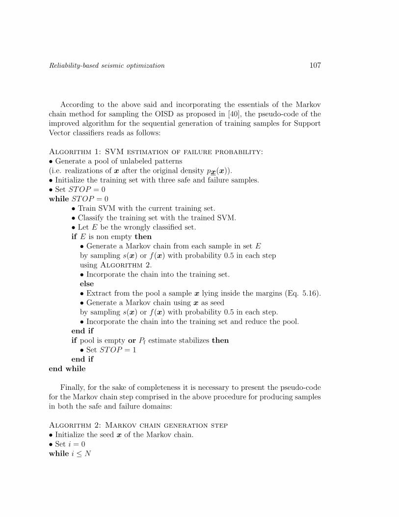
Reliability-based seismic optimization 107
According to the above said and incorporating the essentials of the Markovchain method for sampling the OISD as proposed in [40], the pseudo-code of theimproved algorithm for the sequential generation of training samples for SupportVector classifiers reads as follows:
Algorithm 1: SVM estimation of failure probability:
• Generate a pool of unlabeled patterns(i.e. realizations of x after the original density px(x)).• Initialize the training set with three safe and failure samples.• Set STOP = 0while STOP = 0
• Train SVM with the current training set.• Classify the training set with the trained SVM.• Let E be the wrongly classified set.if E is non empty then
• Generate a Markov chain from each sample in set Eby sampling s(x) or f(x) with probability 0.5 in each stepusing Algorithm 2.• Incorporate the chain into the training set.else
• Extract from the pool a sample x lying inside the margins (Eq. 5.16).• Generate a Markov chain using x as seedby sampling s(x) or f(x) with probability 0.5 in each step.• Incorporate the chain into the training set and reduce the pool.
end if
if pool is empty or Pf estimate stabilizes then
• Set STOP = 1end if
end while
Finally, for the sake of completeness it is necessary to present the pseudo-codefor the Markov chain step comprised in the above procedure for producing samplesin both the safe and failure domains:
Algorithm 2: Markov chain generation step
• Initialize the seed x of the Markov chain.• Set i = 0while i ≤ N

108 Reliability problems in Earthquake Engineering
• Set i = i + 1• Generate a sample ξ from the Uniform densityin a hyperbox of widths Ld, d = 1, 2, . . . , D (Eq. 5.15).• Calculate the limit state function g(ξ)• Calculate the limit state function g(x)(if not already calculated)• Generate a uniform random number w in the range (0, 1).if w ≤ 0.5 then
• Set r = s(ξ)/s(x) (Eq. 5.13)else
• Set r = f(ξ)/f(x) (Eq. 5.13)end if
• Set t = min(r, 1).• Generate a uniform random number v in the range (0, 1).if t ≥ v then
• Accept ξ as the next sample in the chainelse
• Keep x as the next sample in the chain and continueend if
end while
5.2.1 Example 5.1. Two dimensional function
As an illustration on the application of the proposed algorithm, consider the limitstate function
g(x1, x2) = −3.8 + exp(x1 − 1.7) − x2 = 0 (5.17)
where the x1, x2 are independent standard Normal variables, drawn from [15]. Theproblem was solved using the homogeneous polynomial kernel of degree 3, whichhas been found very useful in structural reliability applications, as it does not needparameters to tune. The chain length was set N = 3 in all cases. Figure 5.3 showsthe initial Markov chains generated in the analysis. It is observed that they wanderin the important region from the classification point of view. Figure 5.4 displaysthe entire training set together with the final support vectors. Notice the balanceddistribution of the samples amongst the safe and failure classes. On the otherhand Figure 5.5 displays the entire history of support vectors. Comparing thelast two figures it can be observed the sequential approach of the support vectors

Reliability-based seismic optimization 109
−6 −4 −2 0 2 4 6−6
−4
−2
0
2
4
6Initial chains
x1
x 2
Figure 5.3: Initial Markov chains for Example 1.
to the actual class boundary. Also, it is important to note that while the endnumber of training samples is 39 the total number of g− function calls is 102, dueto the use of the Markov chains that implies the rejection of some samples whoseg−value is actually evaluated, as illustrated by the respective algorithm. However,the Markov chain approach assures sampling in the important region, which is avery important prerogative when dealing with implicit limit state functions and,besides, the total number of solver calls is anyhow low. The probability of failurewas calculated with 100,000 using both Monte Carlo simulation and the fittedSVM obtaining the same value (0.0024).

110 Reliability problems in Earthquake Engineering
−6 −4 −2 0 2 4 6−6
−4
−2
0
2
4
6training samples
x1
x 2
Safe samplesFailure samplesSupport vectors
Figure 5.4: Training samples and end support vectors in Example 1.
5.2.2 Example 5.2. Two dimensional function with small
Pf
It must be observed that the estimation of failure probabilities using Support Vec-tor Machines is pretty independent of the value of the failure probability becausethe relevant issue is the availability of samples in both domains, their correspond-ing probability notwithstanding. to show this consider the limit state function[40]
g(x1, x2) =
5 −√
x21 + x2
2 if |x1| ≤ 5/√
2, x2 > 0
5√
2 − |x1| − x2 if |x1| > 5/√
2(5.18)
where the two variables are standard independent Normal. This function has acontour of equal probability so that there is an infinity of points at equal distance

Reliability-based seismic optimization 111
−6 −4 −2 0 2 4 6−6
−4
−2
0
2
4
6Support vector history
x1
x 2
Figure 5.5: Support vector history in Example 5.1.
from the origin making it difficult the application of several structural reliabilitymethods as in the previous case.
The problem was solved with the same SVM as in Example 1. The trainingpopulation and the final support vectors are displayed in Figure 5.6. Consideringthe fact that the shortest distance from the function to the origin is large, thecalculation of the failure probability with Monte Carlo simulation and the trainedSupport Vector Machine was performed with 5,000,000 samples. The results coin-cide at 2 × 10⁻⁶.

112 Reliability problems in Earthquake Engineering
−15 −10 −5 0 5 10 15−15
−10
−5
0
5
10
15training samples
x1
x 2
Safe samples
Failure samples
Support vectors
Figure 5.6: Results of Example 5.2.
5.3 Methodology for RBDO
As stated above, in reliability-based design optimization it is necessary to computeone or several failure probabilities for each trial model, with the consequence thatthe number of calls of the set of equations defining the structural model tends to bevery large. Previous section dealt with a method for reducing such a number of thestructural reliability computations. A similar goal should guide the specificationof the optimization algorithm.
As said in the Introduction, the Particle Swarm method for optimization [151](PSO) has been selected after the benchmark comparison published in [152]. Thoughinspired in biological processes, similarly to Genetic Algorithms and evolutionaryStrategies, PSO differs from them in using as a paradigm the social behavior of

Reliability-based seismic optimization 113
groups of species instead of their evolution. PSO has been successfully applied instructural reliability [156] as well as in structural optimization [157, 158, 159], ,earthquake engineering [95] and others.
Consider several structural models as particles in the y−design space. Themotion of the i -th individual particle in iteration k + 1 to a new position yk+1
i is[151]
yk+1i = yk
i + vk+1i (5.19)
where vk+1i is the so-called velocity given by
vk+1i = χ
(
wvki + Z1r
ki
(
P ki − yk
i
)
+ Z2ski
(
P kg − yk
i
))
, i = 1, 2, . . . , N (5.20)
In this equation the leading roles are those of P ki and P k
g , which are respectively thebest historical position of the i -th particle and the best current position amongstall particles of the group. Parameters Z1 and Z2 are positive constants calledrespectively cognitive and social parameters due to their relationship to P k
i andP k
g . Besides χ is a factor that controls the velocity, w is an inertial weight givingimpulse to the particles, rk
i and ski are random numbers uniformly distributed in
the range [0, 1] that operate a perturbation and N is the population size.The constituting ingredients elements of the algorithm are, therefore, the fol-
lowing:
• The experience of each individual, expressed by(
P ki − yk
i
)
and representingthe direction taken by the particle with respect to its best historical position.
• The experience of the group,(
P kg − yk
i
)
, representing a magnetic vector to-wards the best position recorded by the collective memory.
• The inertia of particles motion, such that a large inertia factor gives impulseto find global solutions while a small factor facilitates finding local minima.Thus it is recommended to initiate the optimization process with a largevalue and decreasing it as the solution advances.
Notice that Eq. (5.20) can be represented as a sum of vectors with directionsvk
i , P ki − yk
i and P kg − yk
i and magnitudes w, Z1rki and z2s
ki , respectively. Such a
sum determines the next position of the particle.The application of this algorithm for RBDO requires handling deterministic and
probabilistic constraints. To this end use is made of a penalty method proposed

114 Reliability problems in Earthquake Engineering
in [160] was used. With reference to Eq. (5.1), it consists in minimizing the costfunction
C1(y) =
C(y) if y ∈ AC(y) + k
√k V (y) if y ∈ U (5.21)
where A is the class of feasible solutions, U that of the unfeasible ones, k is theiteration counter and V (y) a penalization function given by
V (y) =R∑
i=1
Θ(qi(y)) [qi(y)]β(qi(y)) (5.22)
where qi(y) = max0, fi(y), Θ(·) is a multistage penalization functional and β(·)a power functional. Since the components of penalty functions are problem depen-dent [161], the details are exposed in the application example. It is presently morerelevant to discuss the link of this optimization method with the SVM classificationapproach for the specific case of RBDO. Firstly, by noticing that the constraintsdefine a partition of the design variable space into feasible and unfeasible mod-els, it is evident that the advantages of Support Vector Machines can be appliedalso in the y−space, besides the random variable space. These two classifiers areidentified as y−SVM and x−SVM, respectively. At a difference with respect toclassifier in the random variable space, no special considerations are presently in-troduced for training the classifier in the design variable space. Secondly, noticethat the margins of the current SVM in the design variable space provide a meansof focalizing the search driven by the PSO, so that a penalization could be addedfor those particles lying beyond the current margins with the aim of acceleratingconvergence. Therefore, the presence of any constraint in Eq. (5.22) is two-fold:(a) a penalization for exceeding the limiting value and (b) a penalization for lyingbeyond the margins of the y−SVM. Notice that for the specific case of probabilis-tic constraints, the availability of the y−SVM classifier render unnecessary thecalculation of failure probabilities for trial models tested after the classifier hasbeen accurately trained, specifically for those models lying beyond the margins.In particular, if the feasible and unfeasible classes are perfectly separable, whichis the case in many structural problems, the y−SVM can be used for avoiding thecalculation of failure probabilities after having a sufficient number of models forits learning.
The proposed RBDO algorithm is then a three-staged procedure described asfollows:

Reliability-based seismic optimization 115
Algorithm 3: RBDO with SVM in two spaces and PSO
Stage 1:
• Initialize randomly the y PSO population.• Define a number of iterations K• Set k = 0while k < K1
• Set k = k + 1for each particle i = 1, 2 . . . , N :
• Train a x−SVM (Algorithm 1).• Calculate Pf with the x−SVM.
end for
• Apply penalizations to those samples exceeding any constraint• Generate the new population
end while
Stage 2:
• Classify the cumulated populations into feasible and unfeasible classes• Train a SVM for these classes (y−SVM).• Initialize randomly a new y PSO population of size Nabout the best position found in Stage 1.• Set k = 0Stage 3:
while k < K2
• Set k = k + 1for each particle i = 1, 2 . . . , N :
• Classify the particle as feasible or unfeasible with y−SVM.end for
• Update the y−SVM with the cumulated populations.• Apply penalizations to those samples exceeding any constraint,including penalization for lying beyond the current y−SVM margins.• Generate the new population
end while
• Deliver the final population as the result and mark the optimum

116 Reliability problems in Earthquake Engineering
5.4 Earthquake Engineering application exam-
ple
The application of the RBDO concept in Earthquake Engineering implies the con-sideration of random variables corresponding to the structural materials and di-mensions as well as to the ground motion excitation. However, the latter groupis by far the most important because the uncertainty of its variables is typicallymuch larger. For this reason, our interest will be focussed on this uncertaintysource exclusively.
The way of defining the seismic action in probabilistic terms is critical in de-termining the realism but also the complexity of the RBDO solution, even in thecase of linear problems. To illustrate this consider the linear equation of motiongiven by [98]
mu + cu + ku = −mrug (5.23)
where m, c and k are respectively the mass, damping and stiffness matrices,respectively, ug is the ground motion acceleration, r a vector of static responses toa unit static ground motion and u the vector of structural displacement responses.As is well known, several design codes recommend the so-called SRSS solution(square-root of the sum of squares) given by
ui =√
φ2i1b
21 + φ2
i2b22 + . . . φ2
ipb2p (5.24)
where φij is the value of the j−th mode shape in the degree of freedom i, p isthe total number of modes relevant for the calculation and the responses bj areproportional to the design spectrum Sd(ωj, νj):
bj = LjSd(ωj, νj) (5.25)
where ωj and νj are respectively the frequency and damping of the j−th modeshape and Lj is the modal participation factor [98]. At this point it should be saidthat there are several alternatives for incorporating the ground motion uncertain-ties into the design optimization, as follows:
1. Random variables defining the design code spectrum. The most importantof these is the maximum ground acceleration Ag, which is typically definedas that having a 10 percent probability of being exceeded in 50 years. In thisapproach there seems to be no clear way of making random the dominant

Reliability-based seismic optimization 117
frequencies of the ground motion besides altering the periods of intersectingfunctions in a random way, but in most cases this would be meaningless.Anyhow notice that even if only the maximum ground acceleration Ag ismodeled as random, there arises a nonlinear relationship between this vari-able and the estimate of the maximum design displacement, according to Eq.(5.24).
2. Uncertain spectrum defined by means of random vibration theories. In thiscase the ground motion is specified with an evolutionary power spectral den-sity function, for which there are several proposals (see [162, 163, 164]), andthe maximum response of the generic single degree of freedom system bymeans of the theory of the first passage problem [104]. This is a sophis-ticated as well as elegant stochastic formulation of the seismic action, notonly because of the use of stochastic models but also for the consideration ofrandom parameters in it. These parameters are the dominant frequency, thespectral shape, the strong motion duration and the maximum ground accel-eration. The relationship linking these variables and the structural responsesis highly nonlinear, as shown in the sequel.
3. Artificial accelerograms, which may be compatible with a design spectrum ornot. In any case the accelerograms should be generated after the stochasticmodel using the random parameters just mentioned because otherwise the re-alism of this Monte Carlo procedure is doubtful. For this reason the methodinherits the highly nonlinear relationship between the seismic model randomparameters and structural responses and makes it even more complex. Forlinear structures this Monte Carlo procedure allows overcoming the approxi-mations linked to approximate solutions of the first passage problem and theSRSS procedure, among others. This alternative is even more relevant foraccurate solutions in the case of nonlinear systems, as it is obvious.
According to this discussion, it is evident that the last alternative is the mostaccurate, but also the most computationally expensive, for RBDO analysis, whichrequires computation of a large number of failure probabilities. In addition, it im-plies a very large increase of the number of random variables (normally hundredsor thousands) represented by those needed for generating the random signal usedby each Monte Carlo sample. This makes difficult the understanding of the un-certainty propagation inside the structural system. On the contrary, in the secondapproach an adequate description of the problem can be made in terms of only

118 Reliability problems in Earthquake Engineering
three independent random variables and two dependent ones defining the uncer-tain power spectrum, as shown next. In this way the entire uncertainty is lumpedin only three variables, thus allowing a good understanding of the problem of de-signing in a highly uncertain environment. A similar approach has been adoptedin [165] for studying the peak response of MDOF structures.
5.4.1 Stochastic spectrum
The spectral displacement Sd(ω, ν) will be defined in terms of a power spectraldensity model using random vibration theories [104]. The power spectrum adoptedis that of Clough-Penzien given by [98]
G(ω) =ω4
g + 4ν2gω
2gω
2
(ω2g − ω2)2 + 4ν2
gω2gω
2· ω4
(ω2f − ω2)2 + 4ν2
f ω2f ω
2G0 (5.26)
where ωg and νg are parameters associated to the dominant soil mass frequencyand damping, respectively, ωf and νf give the spectrum a necessary decreasingshape in the low frequency region, and G0 is the one-sided power spectrum ofthe underlying white noise. This parameter can be related to the peak groundacceleration Ag by [99, 100]
G0 = 2
(
Ag
28.4
)2
(5.27)
On the other hand the spectral displacement is given by
Sd(ω, ν) = λ(s, R) σu (5.28)
where σu is the standard deviation of the displacement response and λ(s, R) theso-called peak factor, which is a function of the duration of the motion in itsstationary phase s and R the probability of the system to remain below the levelSd(ω, ν) in the interval (0, s). In other words, R is the reliability that the designerintends to confer to the system and thus it is given by R = 1−Q, where Q is thelimiting failure probability in the optimization (see Eq. e2q). The peak factor isapproximately given by
λ(s, R) ≈
√
√
√
√2ln
(
− ωs
πlnR
[
1 − exp
−√
4νsln(
− ωs
πlnR
)
])
(5.29)

Reliability-based seismic optimization 119
where
νs =ν
1 − exp(−2νωs)(5.30)
For the duration of the strong motion phase s, the following regression will beapplied [105, 106]:
s = 30 exp(
−3.254A0.35g
)
(5.31)
Finally, the standard deviation of the displacement can be obtained from thefollowing expression:
σ2u =
1
ω4
ωG(ω)
(
π
4νs− 1
)
+
ω∫
0
G(Ω)dΩ
(5.32)
In this study, the set of basic random variables is defined as
x = ωg, νg, Ag (5.33)
Table 5.1: Probabilistic definition of independent spectral random variables
Parameter Distribution Mean c.o.v.ωg Gamma 20.3 rad/s 0.448νg Lognormal 0.32 0.421Ag Lognormal 0.25 g 0.6
The probabilistic definition of the first two random variables appearing in Table 1follows reference [106]. The peak ground acceleration is modeled as a Lognormalvariable with mean 0.25 g and a coefficient of variation 0.6, according to theresearch reported in [109]. Note that the uncertainty of all these variables is quitelarge, thus making significant the reliability-based optimization of structures inwhich the nonstructural damage as well as the overall stability depends on thelateral displacements. This is evidently more crucial for base isolation systems.It most be noted, however, that the randomness of the peak ground accelerationmay be larger, since according to a study quoted in [81] its coefficient of variationlies in the range from 0.56 to 1.38. In addition, there are two dependent randomvariables, namely G0 and s , given respectively by Eqs. (5.27) and (5.31).

120 Reliability problems in Earthquake Engineering
m
mb
k
kb
ug
ub
u
Figure 5.7: Base isolated building model.
5.4.2 Discussion on a base isolated building case
Seismic base isolation is an interesting case for testing structural reliability con-cepts and methods because of the critical dependence of the overall system safetyon the lateral displacement of the supporting base. In this section the proposedalgorithm for RBDO is applied for optimizing the design of a base isolated buildingsubject to a earthquake design defined by means of random vibration theories.
Consider a two-floor base isolated building depicted in Figure 5.7, whose equa-tions of motion were specified in the previous Chapter.
In order to illustrate the advantages of applying the pattern recognition paradigmin stochastic optimization, which justify the introduction of the y−SVM in Algo-rithm No. 3, one hundred models of this building were randomly generated andanalyzed with the stochastic spectrum described above, using the random variabledefinitions given in Table 1. Each model was identified by the set y = M, ωs, ωb,where M = m+mb with m = 100 t. In order to facilitate visualization, parameterωs was set equal to 13 rad/s. For each model the probability of exceeding 0.02 m

Reliability-based seismic optimization 121
80 90 100 110 120 130 140 150 160 170 1800
1
2
3
4
5
6
7
8
9y−SVM
M
ωb
−1
−1 −1
0
0 00
1
1 1
Feasible modelsUnfeasible models
Figure 5.8: Two dimensional SVM fitted in y space for feasible and unfeasibledomains.
by the base displacement vb, considered as the failure condition, was calculatedusing 5,000 samples of the random variable set x = ωg, νg, Ag. Finally, the mod-els were labeled as feasible if their failure probability was lower than or equal to0.03 and unfeasible otherwise and a SVM with polynomial kernel of degree 3 wastrained with the labeled samples. The result is displayed in Figure 5.8. It canbe seen that the SVM can be confidently used to avoid the costly calculation ofthe failure probability of each model after a sufficient number of samples allows itsadequate training. In this respect it must be noted that the optimal characteristicsof the SVM allow a reasonably good generalization capacity (i.e. high probabilityof correct class prediction for samples not used in the training phase) when trainedwith a reduced number of samples. This is an involved subject for which the in-

122 Reliability problems in Earthquake Engineering
terested reader is referred to [56, 15]. In addition, the margins of the y−SVM canbe used for restricting the search space of the PSO algorithm, as explained in thepreceding.
5.4.3 RBDO of a base isolated building
For the base isolated building model depicted in Figure 5.7 the RBDO problem isdefined as follows:
find : y
minimizing : C(y) = y1 + 1π2 (y2
2 + 2y23) (5.34)
subject to : P[0.035m − max |vb| ≤ 0] ≤ 0.03 (5.35)
ωs ≥ 11rad/s (5.36)
where
y = y1, y2, y3 = M, ωs, ωb (5.37)
In words, the goal is to minimize a cost function construed as the base slabmass plus the squared structural stiffness and twice the squared base isolationstiffness. The factor for the latter is introduced with a regard to the high costof the isolation devices. The probabilistic constraint corresponds to a restrictionposed on the base displacement to a maximum of 0.035 m, which is judged to bea threshold beyond which the overall stability of the structure is under risk. Thelimiting probability is Q = 0.03. The deterministic constraint corresponds to alimit posed on the natural frequency of the structure to avoid excessive flexibility.
For each calculation of the failure probability use was made of Markov chainswith 10 samples. The three-stage algorithm was applied with K1 = 10, K2 = 10(corresponding respectively to the number of iterations in the first and third stages)and N = 10 particles. The penalization of the constraints corresponds to R = 2in Eq. (5.22) with the following specifications:
q1(y) = max0, (11 − ωs) (5.38)
q2(y) = max0, (Pf − Q) (5.39)
where Pf = P[0.035 − max |vb(x, y)| ≤ 0]. In addition

Reliability-based seismic optimization 123
Θ(q1(y)) =
1 if q1 < 0.0012 if 0.001 ≤ q1 < 0.013 if 0.01 ≤ q1 < 0.14 otherwise
(5.40)
Θ(q2(y)) =
0.1 if q2 < 0.0010.2 if 0.001 ≤ q2 < 0.010.3 if 0.01 ≤ q2 < 0.10.4 otherwise
(5.41)
β(q1(y)) =
1 if q1 < 0.52 otherwise
(5.42)
β(q2(y)) =
1 if q2 < 0.0052 otherwise
(5.43)
However, after the first y−SVM was fitted (i.e. after the first K1 iterations), thepenalization of the probabilistic constraint changed simply to
q2(y) = max0,−c(y)Θ(q2(y)) = 0.03 (5.44)
β(q2(y)) = 2
where c(y) is the label given by the y−SVM to the particle, given by
c(y) = sgn [r(y)] = sgn
[
S∑
k=1
αkckK(y, yk) − b
]
(5.45)
where r(y) measures the distance of the particle y to the discriminating func-tion. Clearly, if the particle is feasible, c(y) = +1, −c(y) = −1, and q2(y) =max0,−c(y) = 0, while the opposite holds for an unfeasible particle. In ad-dition, as said in the preceding, the position of the particle beyond the currenty−SVM margin is penalized in the third stage. To this end use was made of thefollowing penalization:
q3(y) = max0, |r(y)| − 1 (5.46)

124 Reliability problems in Earthquake Engineering
Θ(q3(y)) =
0.001 if q3 < 0.10.01 if 0.1 ≤ q3 < 10.03 otherwise
(5.47)
β(q3(y)) =
1 if q1 < 12 otherwise
(5.48)
The constraint in Eq. (5.46) stems from the fact that a value of |r(y)| greater thatone corresponds to a sample beyond the margin.
0 2 4 6 8 10 12 14 16 18 202
3
4
5
6
7
8
9x 10
7
Iteration No.
Cos
t
Figure 5.9: Evolution of cost function of the base isolated building. (Each linecorresponds to a trial model).

Reliability-based seismic optimization 125
0 2 4 6 8 10 12 14 16 18 2010
−6
10−5
10−4
10−3
10−2
10−1
100
101
102
103
Iteration No.
Pen
aliz
atio
n
Figure 5.10: Evolution of penalization cost for the base isolated building.
Figure 5.9 shows the evolution of the structural cost function C(y) for the tenparticles along the K1 + K2 = 20 iterations. It can be observed that the algo-rithm converges rapidly. The minimum cost corresponds to y = M, ωs, ωb =186.6207t, 11.9679rad/s, 3.2567rad/s. Figure 5.10 shows the total penalizationapplied to the particles. The lines are broken for those particles which at certainiterations are not penalized. Notice that the penalization cost increases and be-comes similar for all particles. Notice also the sudden reduction of the penalizationcost when passing from the first stage to the third. This is not only due to theintroduction of the third constraint concerning the violations of the margins ofthe newly calculated y−SVM, but also to the change of initial population beforestarting the third stage, thus indicating that the generation of a new populationin the vicinity of the best particle arising from the first stage is beneficial. On the

126 Reliability problems in Earthquake Engineering
100
150
200
11
12
13
14
15
16
172
3
4
5
6
Mωs
ωb
initial populationintermediate iterationfinal iteration
Figure 5.11: Snapshots of PSO convergence of base isolated building.
other hand, Figure 5.11 shows that the entire final population cluster in a smallregion close to the limiting value of ωs = 11 rad/s. Finally, Figure 5.12 displays theevolution of the failure probability estimates of all the particles through the firstK1 = 10 iterations. The figure interrupts at this point because of the introductionof the y−SVM, which henceforth reports the feasibility or unfeasibility of the par-ticle with labels +1,−1, respectively, without giving any estimate of the failureprobability. Comparing this Figure with Fig. 5.9, it can be observed that as thecost diminishes the spread of the failure probability also reduces and, at the endof the first stage, almost all failure probabilities become lower than the imposedconstraint. These figures demonstrate that the penalization technique succeeds insubmitting the particles to the constraints.

Reliability-based seismic optimization 127
1 2 3 4 5 6 7 8 9 1010
−4
10−3
10−2
10−1
100
Iteration No.
Pf
Figure 5.12: Evolution of the failure probability of the base isolated building.
5.5 Final remarks
This section is devoted to some comments about the limitations and hurdles of themethodologies proposed in the present paper.
First, with respect to the proposed algorithm for RBDO (Algorithm 3), it isimportant to note that the limiting numbers of iterations K1 and K2 are fixedon heuristic basis according to the international experience in SVM classification.Besides, they are given different names because of the dimensionality of x−SVM isin general different from that of the y−SVM. Alternatively, the proposed algorithmcan be modified by absorbing the training of the y−SVM in Stage 1 and stoppingits training according to a suitable stopping criterion. For instance, when themargin band becomes so narrow that the likelihood of misclassification of new

128 Reliability problems in Earthquake Engineering
samples becomes little.Also, improvements should be made to avoid the tend of flexible learning clas-
sifiers to produce fake twists and sometimes loops that may affect the predictionin both the x− and y−spaces. An alternative using random numbers with a highentropy for the initial population is presently being evaluated by the authors.
Finally, in all uses of flexible classifiers it is important to incorporate methodsfor selecting its parameters (such as the number of neurons in Neural Networks ofthe kernel parameters in Support Vector Machines). The proposals for performingthis task found in the international literature can be grouped into two categories:(a) the use of resampling techniques, in which several classifiers are evaluated withsubsets of the given training population and (b) optimization techniques for findingthe best parameters. Note that in applying these methods the training populationis the same, so that the only increase in computational cost is that represented bythe application of the resampling or optimization method.

Bibliography
[1] R. L. Iman and W. J. Canover. Small sample sensitivity analysis techniquesfor computer models with an application to risk assessment. Communications
in Statistics, Theory and Methods, A9:1749 – 1842., 1980.
[2] A. Florian. An efficient sampling scheme: Updated Latin Hypercube Sam-pling. Probabilistic Engineering Mechanics, 7:123 – 130, 1992.
[3] D.E. Huntington and C.S. Lyrintzis. Improvements to and limitations ofLatin Hypercube Sampling. Probabilistic Engineering Mechanics, 13:245 –253, 1998.
[4] K. Ziha. Descriptive sampling in structural safety. Structural Safety, 17:33– 41, 1995.
[5] A. Harbitz. An efficient sampling method for probability of failure calcula-tion. Structural Safety, 3:109 – 115., 1986.
[6] G. I. Schueller, C. G. Bucher, U. Bourgund, and W. Ouypornprasert. On ef-ficient computational schemes to calculate failure probabilities. Probabilistic
Engineering Mechanics, 4:10 – 18, 1989.
[7] O. Ditlevsen and H. O. Madsen. Structural Reliability Methods. John Wileyand Sons, Chichester, 1996.
[8] S. K. Au and J. L. Beck. Estimation of small failure probabilites in high di-mensions by subset simulation. Probabilistic Engineering Mechanics, 16:263– 277, 2001.
[9] A. Olsson, G. Sandberg, and O. Dahlblom. On Latin Hypercube samplingfor structural reliability analysis. Structural Safety, 25:47–68, 2003.
129

130 Reliability problems in Earthquake Engineering
[10] S. K. Au and J. L. Beck. Importance sampling in high dimensions. Structural
Safety, 25:139 – 163, 2003.
[11] G. E. P. Box and N. R. Draper. Empirical Model Building and Response
Surfaces. John Wiley and Sons, New York, 1987.
[12] D. C. Montgomery. Design and Analysis of Experiments. John Wiley andSons, New York, 1991.
[13] J. E. Hurtado. Analysis of one-dimensional stochastic finite elements usingneural networks. Probabilistic Engineering Mechanics, 17:35 – 44, 2002.
[14] J. E. Hurtado and D. A. Alvarez. A classification approach for reliabilityanalysis with stochastic finite element modeling. Journal of Structural En-
gineering, 129:1141 – 1149, 2003.
[15] J. E. Hurtado. Structural Reliability. Statistical Learning Perspectives.Springer, Heidelberg, 2004.
[16] J. E. Hurtado and D.A. Alvarez. An optimization method for learning statis-tical classifiers in structural reliability. Probabilistic Engineering Mechanics,25:26 – 34, 2010.
[17] O. Ditlevsen. Principle of Normal tail approximation. Journal of the Engi-
neering Mechanics Division, 107:1191 – 1207, 1981.
[18] R. Rackwitz and B. Fiessler. Structural reliability under combined loadsequences. Computers and Structures, 9:489 – 494, 1978.
[19] M. Hohenblicher and R. Rackwitz. Non-normal dependent vectors in struc-tural reliability. Journal of the Engineering Mechanics Division, 107:1127 –1138, 1981.
[20] S. Kotz, N. Balakrishnan, and N. L. Johnson. Continuous Multivariate Dis-
tributions, Vol. 1. John Wiley and Sons, New York, 2000.
[21] A. Nataf. Determination des distributions dont les marges sont donees.Comptes rendues de l’Academie des Sciences, 225:42–43, 1962.
[22] P. L. Liu and A. DerKiureghian. Multivariate distribution models withprescribed marginals and covariances. Probabilistic Engineering Mechanics,1:105 – 112, 1986.

Reliability-based seismic optimization 131
[23] H. J. Pradlwarter, C. G. Bucher, and G. I. Schueller. Nonlinear systems. InG. I. Schueller, editor, Structural Dynamics: Recent Advances, pages 128 –213. Springer-Verlag, Berlin, 1991.
[24] A. DerKiureghian, H. Z. Lin, and S. J. Hwang. Second-order reliabilityapproximations. Journal of Engineering Mechanics, 113:1208–1225, 1987.
[25] Y. G. Zhao and T. Ono. New approximations for SORM: Part I. Journal of
Engineering Mechanics, 125:79–85, 1999.
[26] A. Haldar and S. Mahadevan. Reliability Assessment using Stochastic Finite
Element Analysis. John Wiley and Sons, New York, 2000.
[27] W. K. Liu, T. Belytschko, and Y. J. Lua. Probabilistic finite element method.In C. (Raj) Sundararajan, editor, Probabilistic Structural Mechanics Hand-
book, pages 70–105. Chapman & Hall, New York, 1995.
[28] R. G. Ghanem and P. D. Spanos. Stochastic Finite Elements: A Spectral
Approach. Springer Verlag, New York, 1991.
[29] B. Sudret and A. DerKiureghian. Stochastic finite element methods andreliability. a state-of-the-art report. Technical report, Report UCB/SEMM-2000/08, Department of Civil and Environmental Engineering, University ofCalifornia, Berkely, 2000.
[30] G. I. Schueller and R. Stix. A critical appraisal of methods to determinefailure probabilities. Structural Safety, 4:293 – 309, 1987.
[31] J. C. Mitteau. Error evaluations for the computation of failure probability instatic structural reliability problems. Probabilistic Engineering Mechanics,14:119 – 135, 1999.
[32] Y. G. Zhao and T. Ono. A general procedure for first/second-order reliabilitymethod (FORM/SORM). Structural Safety, 21:955 – 112, 1999.
[33] Y. G. Zhao and T. Ono. New approximations for SORM: Part II. Journal
of Engineering Mechanics, 125:86–93, 1999.
[34] R. Y. Rubinstein. Simulation and the Monte Carlo Method. John Wiley andSons, New York, 1981.
132 Reliability problems in Earthquake Engineering
[35] R. E. Melchers. Structural Reliability: Analysis and Prediction. John Wileyand Sons, Chichester, 1999.
[36] C. G. Bucher, H. J. Pradlwarter, and G. I. Schueller. Computational stochas-tic structural analysis. In G. I. Schueller, editor, Structural Dynamics: Recent
Advances, pages 285 – 300. Springer-Verlag, Berlin, 1991.
[37] R. E. Melchers. Importance sampling in structural systems. Structural
Safety, 6:3 – 10, 1989.
[38] G. L. Ang, A. H-S. Ang, and W. H. Tang. Optimal importance samplingdensity estimator. Journal of Engineering Mechanics, 118:1146 – 1163, 1991.
[39] C. G. Bucher. Adaptive Sampling: An Iterative Fast Monte-Carlo Procedure.Structural Safety, 5:119 – 126., 1988.
[40] S. K. Au and J. L. Beck. A new adaptive importance sampling scheme forreliability calculations. Structural Safety, 21:135 – 158, 1999.
[41] C. P. Robert and G. Casella. Monte Carlo Statistical Methods. Springer,New York, 1999.
[42] D. W. Scott. Multivariate density estimation. John Wiley and Sons, NewYork, 1992.
[43] G. McLachlan and D. Peel. Finite Mixture Models. John Wiley and Sons,New York, 2000.
[44] P. Bjerager. Methods for structural reliability computation. In F. Cas-ciati and J. B. Roberts, editors, Reliability Problems: General principles and
Applications in Mechanics of Solids and Structures, pages 89–136. Springer-Verlag, Wien, 1991.
[45] J. S. Liu. Monte Carlo Strategies in Scientific Computing. Springer, NewYork, 2001.
[46] H. J. Pradlwarter and G. I. Schueller. Assessment of low probability eventsof dynamical systems by controlled Monte Carlo simulation. Probabilistic
Engineering Mechanics, 14:213 – 227, 1999.

Reliability-based seismic optimization 133
[47] N. Harnpornchai, H. J. Pradlwarter, and G. I. Schueller. Stochastic anal-ysis of dynamical systems by phase-space controlled Monte Carlo simula-tion. Computer Methods in Applied Mechanics and Engineering, 168:273–283, 1999.
[48] P. G. Melnik-Melnikov and E. S. Dekhtyaruk. Rare events probabilitiesestimation by “Russian Roulette and Splitting” simulation technique. Prob-
abilistic Engineering Mechanics, 15:125 – 129, 2000.
[49] C. Bucher. A fast and efficient response surface approach for structuralreliability problems. Structural Safety, 7:57–66, 1990.
[50] L. Faravelli. Response-surface approach for reliability analysis. Journal of
the Engineering Mechanics, 115:2763 – 2781, 1989.
[51] M. R. Rajashekhar and B. R. Ellingwood. A new look at the response surfaceapproach for reliability analysis. Structural Safety, 12:205–220, 1993.
[52] S. H. Kim and S. W. Na. Response surface method using vector projectedsampling points. Structural Safety, 19:3–19, 1997.
[53] X. L. Guan and R.E. Melchers. Effect of response surface parameter variationon structural reliability estimates. Structural Safety, 23:429 – 444, 2001.
[54] J. E. Hurtado and D. A. Alvarez. Neural network-based reliability anal-ysis: A comparative study. Computer Methods in Applied Mechanics and
Engineering, 191:113 – 132, 2001.
[55] C. M. Bishop. Neural Networks for Pattern Recognition. Oxford UniversityPress, Oxford, 1995.
[56] V. N. Vapnik. Statistical Learning Theory. John Wiley and Sons, New York,1998.
[57] M. Papadrakakis, V. Papadopoulos, and N.D. Lagaros. Structural relia-bility analysis of elastic-plastic structures using neural networks and MonteCarlo simulation. Computer Methods in Applied Mechanics and Engineering,136:145 – 163, 1996.
134 Reliability problems in Earthquake Engineering
[58] T. Sasaki. A neural network-based response surface approach for comput-ing failure probabilities. In R. B. Corotis, G. I. Schueller, and M. Shi-nozuka, editors, Structural Safety and Reliability - Proceedings of the In-
ternational Conference on Structural Safety and Reliability, ICOSSAR 01,
Newport Beach, California, 17-22 June 2001, page 257, Lisse, The Nether-lands, 2001. A.A.Balkema, Publishers.
[59] S. V. S. Cabral and L. S. Katafygiotis. Neural network based response sur-face method and adaptive importance sampling for reliability analysis oflarge structural systems. In R. B. Corotis, G. I. Schueller, and M. Shi-nozuka, editors, Structural Safety and Reliability - Proceedings of the In-
ternational Conference on Structural Safety and Reliability, ICOSSAR 01,
Newport Beach, California, 17-22 June 2001, page 46, Lisse, The Nether-lands, 2001. A.A.Balkema, Publishers.
[60] J. E. Hurtado. Neural networks in stochastic mechanics. Archives of Com-
putational Methods in Engineering, 8:303 – 342, 2001.
[61] A. Sen and M. Srivastava. Regression Analysis. Springer Verlag, New York,1990.
[62] B. D. Ripley. Pattern Recognition and Neural Networks. Cambridge Univer-sity Press, Cambridge, 1996.
[63] B. Scholkopf and A. Smola. Learning with Kernels. The M. I. T. Press,Cambridge, 2002.
[64] K. Sobczyk and J. Trebicki. Maximum entropy principle in stochastic dy-namics. Probabilistic Engineering Mechanics, 5:102 – 110, 1990.
[65] J. Trebicki and K. Sobczyk. Maximum entropy principle and non-stationarydistributions of stochastic systems. Probabilistic Engineering Mechanics,11:169–178, 1996.
[66] J. E. Hurtado and A.H. Barbat. Fourier-based maximum entropy method instochastic dynamics. Structural Safety, 20:221 – 235, 1998.
[67] G. K. Er. A method for multi-parameter PDF estimation of random vari-ables. Structural Safety, 20:25 – 36, 1998.

Reliability-based seismic optimization 135
[68] C. A. Kennedy and W. C. Lennox. Solution to the practical problem ofmoments using non-classical orthogonal polynomials with applications forprobabilistic analysis. Probabilistic Engineering Mechanics, 15:371 – 379,2000.
[69] C. A. Kennedy and W. C. Lennox. Moment operations on random vari-ables, with applications for probabilistic analysis. Probabilistic Engineering
Mechanics, 16:253 – 259, 2001.
[70] G. A. Athanassoulis and P. N. Graviladis. The truncated hausdorff momentproblem solved with kernel density functions. Probabilistic Engineering Me-
chanics, 17:273 – 291, 2002.
[71] H. P. Hong and N. C. Lind. Approximate reliability analysis using normalpolynomial and simulation results. Structural Safety, 18:329 – 339., 1996.
[72] A. M. Hasofer. Non-parametric estimation of failure probabilities. In F. Cas-ciati and B. Roberts, editors, Mathematical Models for Structural Reliability
Analysis, pages 195–226. CRC Press, Boca Raton, 1996.
[73] Y. G. Zhao and T. Ono. Moment methods for structural reliability. Structural
Safety, 23:47 – 75, 2001.
[74] L. Xu and G. Cheng. Discussion on: moment methods for structural relia-bility. Structural Safety, 25:193 – 199, 2003.
[75] M. L. Shooman. Probabilistic Reliability: An Engineering Approach.McGraw-Hill, New York, 1968.
[76] M. E. Harr. Reliability-based Design in Civil Engineering. Dover Publica-tions, New York, 1987.
[77] E. T. Jaynes. Information Theory and Statistical Mechanics. The Physical
Review, 106:620 – 630, 1957.
[78] F. M. Reza. An Introduction to Information Theory. Dover Publications,New York, 1994.
[79] A. Papoulis. Probability, Random Variables and Stochastic Processes.McGraw-Hill, New York, 1991.

136 Reliability problems in Earthquake Engineering
[80] F. Grooteman. Adaptive radial-based importance sampling method for struc-tural reliability. Structural Safety, 30:533 – 542, 2008.
[81] R. D. Bertero and V. V. Bertero. Performance-based seismic engineering:the need for a reliable conceptual comprehensive approach. Earthquake En-
gineering and Structural Dynamics, 31:627 – 652, 2002.
[82] R. G. Sexsmith. Probability-based safety analysis – value and drawbacks.Structural Safety, 21:303 – 310, 1999.
[83] I. Elishakoff. Safety Factors and Reliability: Friends or Foes? Kluwer, NewYork, 2005.
[84] I. Doltsinis and A. Kang. Robust design of structures using optimiza-tion methods. Computer Methods in Applied Mechanics and Engineering,193:2221 – 2237, 2004.
[85] H. G. Beyer and B. Sendhoff. Robust Optimization. A comprehensive survey.Computer Methods in Applied Mechanics and Engineering, 196:3190–3218,2007.
[86] E. Rosenblueth and E. Mendoza. Reliability optimization in isostatic struc-tures. Journal of the Engineering Mechanics Division ASCE, 97:1625–1640,1971.
[87] M. Gasser and G. I. Schueller. Reliability-based optimization of structuralsystems. Mathematical Methods of Operations Research, 46:287–307, 1997.
[88] N. C. Nigam and S. Narayanan. Applications of Random Vibrations. SpringerVerlag - Narosa Publishing House, Berlin, New Delhi, 1994.
[89] D. Frangopol. Reliability-based structural design. In C. (Raj) Sundararajan,editor, Probabilistic Structural Mechanics Handbook, pages 352–387. Chap-man & Hall, New York, 1995.
[90] B. Ellingwood, J. C. MacGregor, and C. A. Cornell. Probability-based loadcriteria: load factors and load combinations. Journal of Structural Engineer-
ing, 108:978–997, 1982.
[91] Y. Ben-Haim. Robust Reliability in the Mechanical Sciences. Springer Verlag,Berlin, 1996.

Reliability-based seismic optimization 137
[92] M. Papadrakakis, N.D. Lagaros, and Y. Tsompanakis. Structural optimiza-tion using evolution strategies and neural networks. Computer Methods in
Applied Mechanics and Engineering, 156:309 – 333, 1998.
[93] N. Lagaros, M. Papadrakakis, and G. Kokossalakis. Structural optimizationusing evolutionary algorithms. Computers and Structures, 80:571–579, 2002.
[94] N. Lagaros and M. Papadrakakis. Soft computing methodologies for struc-tural optimization. Applied Soft Computing, 3:283–300, 2003.
[95] J. E. Hurtado. Optimal reliability-based design using support vector ma-chines and artificial life algorithms. In Y. Tsompanakis and N. D. Lagaros,editors, Intelligent Computational Paradigms in Earthquake Engineering.Idea Group Inc., Hershey, 2006.
[96] I. Doltsinis, A. Kang, and G. Cheng. Robust design of non-linear structuresusing optimization methods. Computer Methods in Applied Mechanics and
Engineering, 194:1779 – 1795, 2005.
[97] J. O. Royset, A. Der Kiureghian, and E. Polak. Reliability-based optimalstructural design by the decoupling approach. Reliability Engineering and
System Safety, 73:213–221, 2001.
[98] R. W. Clough and J. Penzien. Dynamics of Structures. McGraw-Hill, NewYork, 1993.
[99] P. Moayyad and B. Mohraz. A study of power spectral density of earth-quake accelerograms. Technical report, Civil and Mechanical EngineeringDepartment, Southern Methodist University, Dallas, TX, 1982.
[100] R. H. Sues, Y. K. Wen, and A. H. S. Ang. Stochastic evaluation of seismicstructural performance. Journal of Structural Engineering, 111:1204–1218,1985.
[101] N. C. Nigam. Introduction to Random Vibrations. The M. I. T. Press,Cambridge, 1983.
[102] T. T. Soong and M. Grigoriu. Random Vibration of Structural and Mechan-
ical Systems. Prentice Hall, Englewood Cliffs, 1993.
[103] L. D. Lutes and S. Sarkani. Stochastic Analysis of Structural and Mechanical
Vibrations. Prentice Hall, Upper Saddle River, 1997.

138 Reliability problems in Earthquake Engineering
[104] E. Vanmarcke. Structural response to earthquakes. In C. Lomnitz andE. Rosenblueth, editors, Seismic Risk and Engineering Decisions, pages 287–337. Elsevier, Amsterdam, 1976.
[105] E. H. Vanmarcke and S. P. Lai. Strong-motion duration and rms amplitudeof earthquake records. Bulletin of the Seismological Society of America,70:1293–1307, 1980.
[106] S. P. Lai. Statistical characterization of strong ground motions using powerspectral density function. Bulletin of the Seismological Society of America,72:259–274, 1982.
[107] M. Shinozuka and Y. Sato. Simulation of nonstationary random processes.Journal of Engineering Mechanics, 93:11–40, 1967.
[108] M. Amin and A. H. S. Ang. A nonstationary stochastic model for strongmotion earthquakes. Technical report, Structural Research Series, 306, Dept.of Civil Engineering, University of Illinois, Urbana-Champaign, Illinois, 1966.
[109] K.A. Ahmed, J. Kanda, and R. Iwasaki. Estimation of uncertainties in thedynamic response of urban soils in Japan. In Proceedings of the Eleventh
World Conference on Earthquake Engineering, Rotterdam, 1996. ElsevierScience.
[110] J. B. Roberts and P. D. Spanos. Random Vibration and Statistical Lineariza-
tion. John Wiley and Sons, Chichester, 1990.
[111] F. Casciati and L. Faravelli. Fragility Analysis of Complex Structural Sys-
tems. Research Studies Press Ltd., Taunton, 1991.
[112] L. Socha. Linearization Methods for Stochastic Dynamic Systems. Springer,Berlin, 2008.
[113] C. A. Schenk and G. I. Schueller. Uncertainty Assessment of Large Finite
Element Systems. Springer, Berlin, 2005.
[114] Y. K. Wen. Method for random vibration of hysteretic systems. Journal of
the Engineering Mechanics Division, 102:248–262, 1976.
[115] T. S. Atalik and S. Utku. Stochastic linearization of multi-degree of free-dom non-linear systems. Earthquake Engineering and Structural Dynamics,4:411–420, 1976.

Reliability-based seismic optimization 139
[116] J. E. Hurtado and A.H. Barbat. Equivalent linearization of the Bouc-Wenhysteretic model. Engineering Structures, 20:1121 – 1132, 2000.
[117] K. Kimura, H. Yasumuro, and M. Sakata. Non-gaussian equivalent lineariza-tion for nonstationary random vibration of hysteretic system. Probabilistic
Engineering Mechanics, 9:15–22, 1994.
[118] J. N. Yang and S. C. Liu. Distribution of maximum and statistical responsespectra. Journal of Engineering Mechanics, 107:1089–1102, 1981.
[119] L. Socha. The sensitivity analysis of stochastic non-linear dynamical systems.Journal of Sound and Vibration, 110:271 – 288, 1986.
[120] L. Socha and G. Zasucha. The sensitivity analysis of stochastic hystereticdynamic systems. In P. D. Spanos and C. A. Brebbia, editors, Computational
Stochastic Mechanics, pages 71–80. Elsevier Applied Science, London, 1991.
[121] E. Rosenblueth. Point estimates for probability moments. Proceedings of the
National Academy of Sciences of the USA, 72:3812 – 3814, 1975.
[122] H. P. Hong, J. A. Escobar, and R. Gomez. Probabilistic assessment of thein seismic response of structural asymmetric models. In Proceedings of the
Tenth European Conference on Earthquake Engineering, Paris, 1998, Rot-terdam, 1998. Balkema.
[123] Y. G. Zhao, T. Ono, and H. Idota. Response uncertainty and time-variantreliability analysis for hysteretic MDF structures. Earthquake Engineering
and Structural Dynamics, 28:1187 – 1213, 1999.
[124] J. E. Hurtado. Structural robustness and its relationship to reliability. InY. Tsompanakis, N. D. Lagaros, and M. Papadrakakis, editors, Structural
Design Optimization Considering Uncertainties. Taylor and Francis, Leiden,2007.
[125] M. Ordaz. On the use of probability concentrations. Structural Safety, 5:317– 318, 1988.
[126] J. T. Christian and G. B. Baecher. Point-estimate method and numeri-cal quadrature. Journal of Geotechnical and Geoenvironmental Engineering,125:779 – 786, 1998.

140 Reliability problems in Earthquake Engineering
[127] M.E. Harr. Probabilistic estimates for multivariate analysis. Applied Math-
emathical Modelling, 13:313 – 318, 1989.
[128] H. P. Hong. An efficient point estimate method for probabilistic analysis.Reliability Engineering and System Safety, 59:261–267., 1998.
[129] J. Ohser and F. Mucklich. Statistical analysis of microstructures in materials
science. John Wiley and Sons, Chichester, 2000.
[130] W. H. Press, S. A. Teukolsky, W. T. Vetterling, and B. P. Flannery. Nu-
merical Recipes in FORTRAN. Cambridge University Press, Cambridge,1992.
[131] J. M. Kelly. Earthquake-Resistance Design with Rubber. Springer-Verlag,London, 1993.
[132] J. H. Lee and B. M. Kwak. Reliability-based structural optimal design usingthe Neumann expansion technique. Computers and Structures, 55:287 – 296,1995.
[133] R. V. Grandhi and L. Wang. Reliability-based structural optimization usingimproved two-pont adaptive nonlinear approximations. Finite Elements in
Analysis and Design, 29:35–48, 1998.
[134] X. Qu and R. T. Haftka. Reliability-based design optimization using prob-abilistic sufficiency factor. Structural and Multidisciplinary Optimization,27:314–325, 2004.
[135] J. O. Royset and E. Polak. Reliability-based optimal design using sampleaverage approximations. Probabilistic Engineering Mechanics, 19:331–343,2004.
[136] J. O. Royset and E. Polak. Reliability-based design optimization of structuralsystems. In Proceedings of the 9th ASCE Speciality Conference on Proba-
bilistic Mechanics and Structural Reliability, Albuquerque, 2004. ASCE.
[137] K. K. Choi, J. Tu, and Y. H. Park. Extension of design potential conceptfor reliability-based design optimization to nonsmooth and extreme cases.Structural and Multidisciplinary Optimization, 22:335–350, 2001.

Reliability-based seismic optimization 141
[138] H. Argawal and J. E. Renaud. Decoupled methodology for probabilisticdesign optimization. In Proceedings of the 9th ASCE Speciality Conference
on Probabilistic Mechanics and Structural Reliability, Albuquerque, 2004.ASCE.
[139] Y. Tsompanakis and M. Papadrakakis. Robust and efficient methods forreliability-based structural optimization. In IASS-IACM 2000 Computa-
tional Methods for Shell and Spatial Structures, ATHENS, 2000. ISASR-NTUA.
[140] C. Papadimitriou and E. Notsios. Robust reliability-based optimization instructural dynamics using evolutionary algorithms. In Proceedings of the
9th ASCE Speciality Conference on Probabilistic Mechanics and Structural
Reliability, Albuquerque, 2004. ASCE.
[141] J. E. Hurtado. Optimal reliability-based design using support vector ma-chines and artificial life algorithms. In Y. Tsompanakis and N. D. Lagaros,editors, Intelligent Computational Paradigms in Earthquake Engineering.Idea Group Inc., Hershey, 2006.
[142] I. Kaymaz and C. A. McMahon. A probabilistic design system for reliability-based design optimization. Structural and Multidisciplinary Optimization,28:416–426, 2004.
[143] M. Kleiber, A. Siemaszko, and R. Stocki. Interactive stability-orientedreliability-based design optimization. Computer Methods in Applied Me-
chanics and Engineering, 168:243 – 253, 1999.
[144] G. Kharmanda, N. Olhoff, A. Mohamed, and M. Lemaire. Reliability-based topology optimization. Structural and Multidisciplinary Optimization,26:295–307, 2004.
[145] B. F. Spencer, M. K. Sain, C. H. Won, D. C. Kaspari, and P. M. Sain.Reliability-based measures of structural control robustness. Structural
Safety, 15:111–129, 1994.
[146] M. Allen and K. Maute. Reliability-based optimization of aerolastic struc-tures. Structural and Multidisciplinary Optimization, 27:228–242, 2004.

142 Reliability problems in Earthquake Engineering
[147] S. Barakat, K. Bani-Hani, and M. Q. Taha. Multi-objective reliability-basedoptimization of prestressed concrete beams. Structural Safety, 26:311–342,2006.
[148] J. E. Hurtado. An examination of methods for approximating implicit limitstate functions from the viewpoint of statistical learning theory. Structural
Safety, 26:271 – 293, 2004.
[149] J. E. Hurtado, F. Zrate, and E. Oate. Reliability estimation of the sheetstamping process using support vector machines. International Journal of
Vehicle Design, 39(1-2):110–124, 2005.
[150] J. E. Hurtado. Filtered importance sampling with support vector margin: apowerful method for structural reliability analysis. Structural Safety, 29:2 –15, 2007.
[151] J. Kennedy and R. C. Eberhart. Swarm Intelligence. Morgan Kaufmann,San Francisco, 2001.
[152] E. Ebeltagi, T. Hegazi, and D. Grierson. Comparison among fiveevolutionary-based optimization algorithms. Information Sciences, 19:43–53, 2005.
[153] Y. K. Wen. Building reliability and code calibration. Earthquake Spectra,11:269–296, 1995.
[154] N. Metropolis, A. W. Rosenbluth, M. N. Rosenbluth, A. H. Teller, andE. Teller. A new algorithm for adaptive multidimensional integration. Jour-
nal of Chemical Physics, 21:1087 – 1092, 1953.
[155] Simon Tong and Daphne Koller. Support vector machine active learningwith applications to text classification. In Pat Langley, editor, Proceedings
of ICML-00, 17th International Conference on Machine Learning, pages 999–1006, Stanford, 2000. Morgan Kaufmann Publishers, San Francisco.
[156] C. Elegbede. Structural reliability assessment based on particle swarm opti-mization. Structural Safety, 27:171 – 186, 2005.
[157] P. C. Fourie and A. A. Groenwold. The particle swarm optimization al-gorithm in size and shape optimization. Structural and Multidisciplinary
Optimization, 23:259–267, 2002.

Reliability-based seismic optimization 143
[158] G. Venter and J. Sobieszczanski-Sobieski. Multidisciplinary optimization ofa transport aircraft wing using particle swarm optimization. Structural and
Multidisciplinary Optimization, 26:121–131, 2004.
[159] J.F. Schutte and A.A. Groenwold. Sizing design of truss structures usingparticle swarms. Structural and Multidisciplinary Optimization, 25:261–269,2003.
[160] K. E. Parsopoulos and M. N. Vrahatis. Particle swarm optimization methodfor constrained optimization problems. Technical report, Department ofMathematics, University of Patras, Greece, 2001.
[161] R. T. Haftka, Z. Gurdal, and M. P. Kamat. Elements of Structural Opti-
mization. Kluwer Academic Publishers, Dordrecht, 1990.
[162] D. M. Boore. Stochastic simulation of high-frequency ground motions basedon seismological models of the radiated spectra. Bulletin of the Seismological
Society of America, 73:18651894, 1983.
[163] G. M. Atkinson ans W. Silva. Stochastic modelling of California groundmotions. Bulletin of the Seismological Society of America, 90:255274, 2000.
[164] C. H. Yeh and Y. K. Wen. Modeling of nonstationary ground motion andanalysis of inelastic structural response. Structural Safety, 8:281–298, 1990.
[165] H. P. Hong and S. S. Wang. Probabilistic analysis of peak response of MDOFsystems with uncertain PSD function. Earthquake Engineering and Struc-
tural Dynamics, 31:1719 – 1733, 2002.

CENTRO INTERNACIONAL DE METODOS NUMERICOS EN INGENIERIA Lista de monografías publicadas en la Serie de Ingeniería Sísmica Las monografías pueden adquirirse dirigiéndose al Departamento de Publicaciones del Centro Internacional de Métodos Numéricos en Ingeniería, Edificio C1, Campus Norte UPC, c/ Gran Capitán s/n, 08034 Barcelona, teléfono: 93-401.60.37, Fax: 93-401-65-17.
IS-1 Qualitative Reasoning for Earthquake Resistant Buildings, Luís M. Bozzo, 149 pp., ISBN 84-87867-36-7, 1993.
IS-2 Control predictivo en sistemas de protección sísmica de estructuras, R. Andrade Cascante, J. Rodellar, F. López Almansa, 143 pp., ISBN 84-87867-37-5, 1993. IS-3 Simulación numérica del comportamiento no lineal de presas de hormigón ante
acciones sísmicas, M. Galindo, J. Oliver, M. Cervera, 255 pp., ISBN 84-87867-38-3, 1994.
IS-4 Simulación del daño sísmico en edificios de hormigón armado, A. Hanganu,
A.H. Barbat, S. Oller, E. Oñate, 96 pp., ISBN 84-87867-40-5, 1994. IS-5 Edificios con aislamiento de base no lineal, N. Molinares, A.H. Barbat, 96 pp.,
ISBN: 84-87867-41-3, 1994. IS-6 Vulnerabilidad sísmica de edificios, C. Caicedo, A.H. Barbat, J.A. Canas,
R. Aguiar, 100 pp., ISBN 84-87867-43-X, 1994. IS-7 Análisis de terremotos históricos por sus efectos, J. R. Arango González, 119 pp., ISBN 84-87867-44-8, 1994. IS-8 Control activo no lineal de edificios con aislamiento de base, A.H. Barbat,
N. Molinares, J. Rodellar, 124 pp., ISBN 84-87867-46-4, 1994. IS-9 Análise estocástica da resposta sísmica nao-linear de estructuras,
A.M. F. Cunha, 199 pp., ISBN: 84-87867-47-2, 1994 IS-10 Definición de la acción sísmica, A.H. Barbat, L. Orosco, J.E. Hurtado,
M. Galindo, 122 pp., ISBN: 84-87867-448-0, 1994 IS-11 Sismología y peligrosidad sísmica, J.A. Canas Torres, C. Pujades Beneit,
E. Banda Tarradellas, 87 pp., ISBN: 84-87867-49-9, 1994 IS-12 Riesgo, peligrosidad y vulnerabilidad sísmica de edificios de mampostería, F. Yépez, A.H. Barbat, J.A. Canas, 104 pp., ISBN: 84-87867-50-2, 1999

IS-13 Estudios de ingeniería sismológica y sísmica, J.A. Canas, ISBN: 84-87867-57-X, 13 pp., 1995 IS-14 Simulación de escenarios de daño para estudios de riesgo sísmico, F. Yépez, A.H. Barbat y J.A. Canas, ISBN: 84-87867-58-8, 103 pp., 1995 IS-15 Diseño sismorresistente de edificios de hormigón armado, L. Bozzo, A.H. Barbat, ISBN: 84-87867-59-6, 185 pp., 1995 IS-16 Modelo tridimensional de atenuación anelástica de las ondas sísmicas en la Península Ibérica, J.O. Caselles, J. A. Canas, Ll. G. Pujades, R.B. Herrmann, ISBN: 84-87867-60-X, 119 pp., 1995 IS-17 Índices de daño sísmico en edificios de hormigón armado, R. Aguiar ISBN: 84-87867-43-X, 99 pp., 1996 IS-18 Experimental study of a reduced scale model seismically base isolated with Rubber-Layer Roller Bearings (RLRB), D. Foti, J.M. Kelly ISBN: 84-87867-82-0, 112 pp., 1996 IS-19 Modelos de evaluación del comportamiento sísmico no lineal de estructuras de hormigón armado, F. Yépez Moya, ISBN: 84-87867-80-4., 96pp., 1996 IS-20 Evaluación probabilista de la vulnerabilidad y riesgo sísmico de estructuras de hormigón armado por medio de simulación, F. Yépez Moya, A.H. Barbat, J.A. Canas, ISBN: 84-87867-81-2, 1996 IS-21 Modelización de la peligrosidad sísmica. Aplicación a Cataluña, J.A. Canas,
J.J. Egozcue, J. Miquel Canet y A.H. Barbat, ISBN: 84-87867-83-9, 101pp., 1996
IS-22 Evaluación del daño sísmico global en edificios porticados de hormigón armado, R. Aguiar, A.H. Barbat and J. Canas, ISBN: 84-87867-96-0, 173pp., 1997 IS-23 Daño sísmico global en edificios con muros de cortante, R. Aguiar, ISBN: 84-89925-00-3, 101 pp., 1997 IS-24 Conceptos de cálculo de estructuras en las normativas de diseño sismorresistente, A.H. Barbat y S. Oller, ISBN: 84-89925-10-0, 107pp., 1997 IS-25 Stochastic dynamics of histeretic structures, J.E. Hurtado, ISBN: 84-89925-09-7, 205pp., 1998

IS-26 Análisis de los acelerogramas de la serie de Adra (Almería). Diciembre 1993 a Enero 1994, R. Blázquez, A. Suárez, E. Carreño y A.J. Martín, ISBN: 84-89925-11-9, 1998
IS-27 Respuesta de puentes frente a acciones sísmicas, E. Maldonado, J.A. Canas,
J.R. Casas, L.G. Pujades, ISBN: 84-89925-23-2, 107pp., 1998 IS-28 Estudio de parámetros en la vulnerabilidad sísmica de puentes, E. Maldonado, J.A. Canas y J.R. Casas, ISBN: 84-89925-16-X, 97pp., 1998 IS-29 Metodologías para o cálculo sísmico não-linear de barragens de betão, R. Faria ISBN: 84-89925-25-9, 113pp., 1998 IS-30 Acciones para el diseño sísmico de estructuras, R. Aguiar, ISBN: 84-89925-27-5, 122pp., 1998 IS-31 Avaliação do comportamento sísmico de barragens de betão, R. Faria, ISBN: 84-89925-28-3, 88pp., 1998 IS-32 Vulnerabilidad sísmica de hospitales. Fundamentos para ingenieros y arquitectos, O.D. Cardona, ISBN:84-89925-33-X, 165pp., 1999 IS-33 Modelación estocástica de la acción sísmica, J. E. Hurtado, ISBN:84-8925-34-8,
93pp., 1999 IS-34 Earthquake simulator testing of a steel model seismically protected with friction energy dissipators, D. Foti and J. Canas, ISBN: 84-89925-40-2, 110pp., 1999 IS-35 Plasticidad y fractura en estructuras aporticadas, J. Flórez López, ISBN: 84-89925-46-1, 90pp., 1999 IS-36 Estimación de efectos locales con movimientos sísmicos y microtemblores,
V. Giraldo, A. Alfaro, L. G. Pujades, J. A. Canas, ISBN: 84-89925-54-2, 83pp., 1999
IS-37 Modelo numérico de elastómeros multi-fase y su aplicación al análisis de
estructuras con aislamiento sísmico, O. Salomón, S. Oller y A. H. Barbat, ISBN: 84-89925-54-2, 239pp.,1999
IS-38 Dinámica de estructuras. Aplicaciones a la Ingeniería Sísmica, J.E. Hurtado, ISBN:84-89925-59-3,177pp., 2000

IS-39 Utilización de los conjuntos difusos en modelos de vulnerabilidad sísmica, E. Maldonado Rondón, J.R. Casas Rius y J.A. Canas, ISBN:84-89925-61-5, 2000
IS-40 Modelo de vulnerabilidad sísmica de puentes basado en " Conjuntos Difusos ",
E. Maldonado Rondón, J.R. Casas Rius, J. A.Canas, ISBN: 84-89925-64-X, 110pp, 2000
IS-41 Vulnerabilidad de puentes de autopista. Un estado del arte, C. Gómez Soberón, A. Barbat, S. Oller, ISBN: 84-89925-64-X, 168pp, 2000
IS-42 Fuerzas sísmicas en los Países Bolivarianos, R. Aguiar Falconí,
ISBN: 84-89925-74-7, 101pp., 2000 IS-43 Espectros de input de energía de aplicación en el proyecto sismorresistente
estructuras en regiones de sismicidad moderada, A. Benavent-Climent, L.G. Pujades, F. López-Almansa, ISBN: 84-89925-86-0, 85 pp., 2001
IS-44 Capacidad límite última de disipación de energía de estructuras de hormigón
Armado sometidas a acciones sísmicas, A. Benavent- Climent, F. López-Almansa, L. G. Pujades, ISBN: 84-89925-88-7, 2001
IS-45 Evaluación del daño en edificios y desempeño sísmico. Programa de ordenador
CEINCI3, R. Aguiar Falconí, ISBN: 84-89925-87-9, 107pp., 2001 IS-46 Estudio analítico sobre el comportamiento sísmico de muros de mampostería
confinada con aberturas, J. J. Álvarez, S.M. Alcocer, ISBN: 84-89925-90-9, 119pp., 2002
IS-47 Seismic vulnerability of bridges using simplified models, C. Gómez Soberón,
S. Oller, A. H. Barbat, ISBN: 84-89925-96-8, 135pp., 2002 IS-48 Control de vibraciones en puentes. Un estado del arte y de la práctica,
M. Jara, J. R. Casas, ISBN: 84-95999-01-3, 120pp., 2002
IS-49 Criterio de diseño de puentes con aisladores y disipadores de energía, M. Jara, J. R. Casas, ISBN: 84-955999-02-1, 115pp., 2002
IS-50 Ferrocemento: Un acercamiento al diseño sísmico, D. A. Bedoya, J. Farbiarz, J. E. Hurtado, Ll. G. Pujades, ISBN: 84-95999-23-4, 76pp., 2002
IS-51 Metodología para la evaluación del desempeño de la gestión del riego,
M. L. Carreño, O. D. Cardona, A. H. Barbat, ISBN: 84-95999-66-8, 2004

IS-52 Sistema de indicadores para la evaluación de riesgos, M. L. Carreño, O. D. Cardona, A. H. Barbat, ISBN: 84-95999-70-6, 200
IS-53 Evaluación “ex-post” del estado de daño en los edificios afectados por un terremoto,
M. L. Carreño, O. D. Cardona, A. H. Barbat, ISBN: 84-95999-76-5, 2005
IS-54 Identificação modal estocástica de estruturas de engenharia civil, F. Magalhães, A. Cunha, E. Caetano, ISBN: 84-95999-89-7, 2005
IS-55 Comportamiento sísmico de puentes articulados y disipación de energia adicional: Un estado del crecimiento, G. E. Valdebenito, A. C. Aparicio, ISBN: 84-95999-87-0, 2005
IS-56 Cálculo y diseño sismorresistente de edificios. Aplicación de la norma NCSE-02, A.H. Barbat, S. Oller and J.C. Vielma, 2005
IS-57 Evaluación rápida de la deriva máxima de piso para calcular la vulnerabilidad sísmica de estructuras, R. Aguiar, ISBN: 84-95999-91-9, 2006
IS-58 Factor de reducción de las fuerzas sísmicas en edificios de hormigón armado sin
muros de corte, R. Aguiar, ISBN: 978-84-96736-40-7, 2007 IS-59 Herramientas necesarias para la evaluación sísmica de edificios, R. Moreno, L.
Pujades, A.C. Aparicio, A.H. Barbat, ISBN: 978-84-96736-53-5, 2007 IS-60 Inelastic Analysis of Geometrically Exact Rods, P. L. Mata, A.H. Barbat, S. Oller,
R. Boroschek, ISBN: 978-84-96736-59-7, 2007 IS-61 La gestión financiera del riesgo desde la perpectiva de los desastres,
M.C.Marulanda, O.D. Cardona, M.G. Ordaz, A.H.Barbat, ISBN:978-84-96736-60-3, 2008
IS-62 Seismic protection of cable-stayed bridges applying fluid viscous dampers, G.E. Valdebenito, A.C. Aparicio, ISBN:978-84-96736-84-9, 2009
Los autores interesados en publicar monografías en esta serie deben contactar con el editor para concretar las normas de preparación del texto.