reliability-based design optimization of offshore wind ...172 l. e. s. stieng and m. muskulus:...
TRANSCRIPT

Wind Energ. Sci., 5, 171–198, 2020https://doi.org/10.5194/wes-5-171-2020© Author(s) 2020. This work is distributed underthe Creative Commons Attribution 4.0 License.
Reliability-based design optimization of offshore windturbine support structures using analytical sensitivities
and factorized uncertainty modeling
Lars Einar S. Stieng and Michael MuskulusDepartment of Civil and Environmental Engineering,
Norwegian University of Science and Technology (NTNU), Trondheim, Norway
Correspondence: Lars Einar S. Stieng ([email protected])
Received: 28 August 2019 – Discussion started: 4 September 2019Revised: 7 November 2019 – Accepted: 15 December 2019 – Published: 29 January 2020
Abstract. The need for cost-effective support structure designs for offshore wind turbines has led to continuedinterest in the development of design optimization methods. So far, almost no studies have considered the effectof uncertainty, and hence probabilistic constraints, on the support structure design optimization problem. In thiswork, we present a general methodology that implements recent developments in gradient-based design opti-mization, in particular the use of analytical gradients, within the context of reliability-based design optimizationmethods. Gradient-based optimization is typically more efficient and has more well-defined convergence prop-erties than gradient-free methods, making this the preferred paradigm for reliability-based optimization wherepossible. By an assumed factorization of the uncertain response into a design-independent, probabilistic partand a design-dependent but completely deterministic part, it is possible to computationally decouple the relia-bility analysis from the design optimization. Furthermore, this decoupling makes no further assumption aboutthe functional nature of the stochastic response, meaning that high-fidelity surrogate modeling through Gaussianprocess regression of the probabilistic part can be performed while using analytical gradient-based methods forthe design optimization. We apply this methodology to several different cases based around a uniform cantileverbeam and the OC3 Monopile and different loading and constraint scenarios. The results demonstrate the via-bility of the approach in terms of obtaining reliable, optimal support structure designs and furthermore showthat in practice only a limited amount of additional computational effort is required compared to deterministicdesign optimization. While there are some limitations in the applied cases, and some further refinement mightbe necessary for applications to high-fidelity design scenarios, the demonstrated capabilities of the proposedmethodology show that efficient reliability-based optimization for offshore wind turbine support structures isfeasible.
1 Introduction
Offshore wind energy is becoming an increasingly compet-itive alternative to the traditional land-based wind farms.However, there remains a level of additional cost which, to-gether with some practical challenges, ensures that offshorewind is still a secondary consideration in many markets.Hence, the reduction of this cost is a primary objective in cur-rent research and development. Cost reduction is generallya multidisciplinary issue, including turbine components like
rotor blades and the drivetrain, wind farm layout, the elec-trical grid and the design of the support structure (includingthe tower). Methods to derive cost-effective, optimal supportstructure designs – balancing minimal use of materials (andpotentially other cost-driving design aspects) with the abilityto safely withstand the loads required by design standards –have been an active area of research for many years. How-ever, very few studies have taken into account the probabilis-tic, fundamentally uncertain aspects of the design process.This includes, for example, uncertainties in the environment
Published by Copernicus Publications on behalf of the European Academy of Wind Energy e.V.

172 L. E. S. Stieng and M. Muskulus: Reliability-based design optimization of offshore wind turbine support structures
and the modeling of the environment, affecting the loads ex-perienced by the structure, as well as uncertainties about thedetails of the design itself, affecting the response to the ap-plied loads. Taking such uncertainties into account generallyrequires the use of probabilistic mathematical methods thatseverely complicate the design optimization problem thatneeds to be solved, both formally and numerically. Hence,deterministic safety factors tend to be used. This is also trueeven for single design assessments. The present study aimsto address these issues by proposing a methodology that al-lows the use of both state-of-the-art optimization methodsrecently developed for support structure design and proba-bilistic assessments of the structural response to both fatigueand extreme loads.
Design optimization of structures subject to probabilisticproblem variables and parameters, sometimes called opti-mization under uncertainty, is in general a large field of re-search at the intersection of two larger fields, optimizationand probabilistic design. One main distinction is betweenrobust design optimization (RBO) (Ben-Tal et al., 2009;Zang et al., 2005) and reliability-based design optimiza-tion (RBDO) (Choi et al., 2007; Valdebenito and Schuëller,2010a). The main difference between the two methods is thatin RBDO the design is optimized normally but under specificprobabilistic limits on structural performance (probability offailure), whereas in RBO the basic idea is to minimize thevariance of a probabilistic objective function in order that theobtained (mean) solution is robust with respect to the uncer-tainties. We will generally restrict our discussion to RBDOand reliability methods but refer to studies on RBO and ro-bust methods where necessary or appropriate. Furthermore,given the extensive research on more general applications ofreliability analysis, optimization and RBDO (or optimizationunder uncertainty more generally), we will focus on previ-ous studies concerning wind turbines. For a more expansiveoverview of structural reliability and RBDO applied to windturbines than the one following below, the interested reader isreferred to Jiang et al. (2017), Leimeister and Kolios (2018),Hübler (2019) and Hu (2018).
A substantial amount of the literature for both structuralreliability analyses and RBDO of offshore wind turbines(OWTs) has focused on aspects other than support struc-ture design. Areas such as blade design (Ronold et al., 1999;Toft and Sørensen, 2011; Dimitrov, 2013; Hu et al., 2016;Caboni et al., 2018), foundation design (Yoon et al., 2014;Carswell et al., 2015; Depina et al., 2016, 2017; Haj et al.,2019; Velarde et al., 2019), component design (Kostandyanand Sørensen, 2011; Rafsanjani et al., 2017; Lee et al., 2014;Li et al., 2017), system/wind farm aspects (Sørensen et al.,2008), inspection and maintenance planning, and probabilis-tic tuning/optimization of safety factors (Sørensen and Tarp-Johansen, 2005; Márquez-Domínguez and Sørensen, 2012;Veldkamp, 2008) have all been studied. As for support struc-ture design specifically, though most structural analyses ofOWTs remain deterministic, there has been a number of stud-
ies incorporating reliability-based (or otherwise probabilis-tic) approaches. For the most part, the reliability-based anal-yses can be divided into two categories. Firstly, there arestudies using simplified probabilistic models where the un-certainty in the response is assumed to be a product of the un-derlying stochastic variables and the deterministic responsevariable (e.g., Thöns et al., 2010; Sørensen and Toft, 2010;Wandji et al., 2016; Yeter et al., 2016, as well as severalof the previously cited studies). Note that the basis for thiskind of factorization can be justified partially or entirely de-pending on both the type of response variable and the typeof stochastic variable. For example, in the case of Yeter et al.(2016), the stochastic variables are mostly either modeling orsimulation errors, or directly originating within the analyticalexpressions for the response variable. Hence, the level of ap-proximation involved in this kind of probabilistic modelingvaries. While not strictly in the same category, studies wherethe fatigue calculation is based on crack propagation mod-els and an assumption that the stress cycles follow a Weibulldistribution, allowing exact limit state expressions to be de-rived, should be mentioned (e.g., Dong et al., 2012). Gen-erally, these simplifications are done in order to be able tosolve the reliability problem using first-/second-order relia-bility methods (FORMs/SORMs) in a computationally fea-sible way. In the second category of studies, the response it-self is simplified, while generally no particular assumptionsabout the stochastic nature of the response are made. Thishas been done through static response modeling (e.g., Weiet al., 2014; Kim and Lee, 2015), but usually the responseis replaced by surrogate models of some kind (e.g., Kolios,2010; Teixeira et al., 2017; Morató et al., 2019). The use ofsurrogate models is often done in order to be able to solve thereliability problem by sampling methods, generally requiringa large number of response evaluations, but surrogate mod-els also make FORM/SORM more computationally practi-cal. Note that this division of reliability methodology is notstrict – Thöns et al. (2010) also makes use of surrogate mod-eling, for example – nor does it cover all approaches, but itis useful as an indicator for one of the fundamental strugglesthat all the aforementioned studies have reckoned with: thefidelity of the probabilistic modeling vs. the fidelity of theunderlying structural analysis.
Only a limited number of studies applying RBDO to OWTsupport structure design have been made. In a series of stud-ies, Yang and collaborators investigated optimization of a tri-pod support structure with probabilistic constraints. In Yanget al. (2015), RBDO was performed, and in Yang and Zhu(2015), RBO was performed. In both cases, a Gaussian pro-cess (kriging) surrogate model was used for the response andMonte Carlo sampling was used for the reliability calcula-tion. In Yang et al. (2018), RBDO was once again performedwith a Gaussian process surrogate model, but in this case thereliability calculation was done using a fractional momentmethod in order to reduce the number of system evaluationsrequired. All three studies used the heuristic optimization
Wind Energ. Sci., 5, 171–198, 2020 www.wind-energ-sci.net/5/171/2020/

L. E. S. Stieng and M. Muskulus: Reliability-based design optimization of offshore wind turbine support structures 173
method called the multi-island genetic algorithm, and the re-liability calculations were done for each step in the optimiza-tion loop, creating a nested two-loop structure. As one mightexpect from a heuristic method, the number of iterations re-quired to solve even the deterministic optimization problem(around 300 iterations) is rather large given the small numberof design variables used, and this is much more pronouncedin the case of the stochastic optimization (around 3000 itera-tions). This means that the method is rather computationallyinefficient, especially considering the number of system eval-uations required by the reliability calculation and the geneticalgorithm at each iteration. However, due to the use of thesurrogate model, this practical issue is overcome, if still ap-parent. Though not an application to OWTs, it is also worthmentioning the study of RBDO applied to offshore mono-pod towers in Karadeniz et al. (2010b) and applied to jacketstructures in Karadeniz et al. (2010a). Here, the limit statefunctions are formulated analytically, and a nested two-loopapproach using gradient-based optimization (in this case se-quential quadratic programming, SQP) and FORM is used.
The previous work on RBDO for OWTs (for both sup-port structures and otherwise) demonstrates that these meth-ods can obtain optimal designs that are both more robust/safewith respect to uncertainties than designs optimized underdeterministic criteria and more tailored to specific designconditions than deterministic designs using safety factors.However, so far (and this is particularly true for supportstructure designs), no studies have taken advantage of recentadvances in deterministic structural optimization methodol-ogy. Optimization methods in general can be divided intogradient-based and gradient-free (often heuristic) methods.Both approaches have been applied to support structure de-sign and other wind turbine components (both on- and off-shore). With some exceptions (e.g., Negm and Maalawi,2000 using an interior penalty method), gradient-free meth-ods were the most common among earlier studies. Examplesinclude Yoshida (2006) using a genetic algorithm, Uys et al.(2007) with a Rosenbrock search and Zwick et al. (2012)with a local scaling of sectional members. The advantages ofthese approaches are that no gradient information is neededfor the optimization, which simplifies the calculations thatneed to be performed for each iteration and avoids the re-liance on finite difference methods, which can be unstablein some implementations. On the other hand, these meth-ods, at least when done at a similar level of detail, gener-ally converge much slower than gradient-based alternatives,where the search for optimal designs can be more specificallyguided by the information provided by the gradients. Withthis disadvantage of gradient-free methods in mind, and seek-ing to avoid the issues related to finite difference methods,some recent studies have demonstrated the viability and, inmost cases, advantages of analytical sensitivities in gradient-based formulations. This has been shown for static (Sandalet al., 2018), quasi-static (Oest et al., 2017) and dynamic(Chew et al., 2016) loading conditions (see also Oest et al.,
2018 for a comparison of these three approaches and a morethorough review of support structure optimization). In gen-eral, these approaches make the design optimization problemmore efficient and stable, though, because of the added con-ceptual complications, these methods have yet to be appliedin studies considering a more realistic and comprehensive setof loading conditions. A study founded on gradient-based op-timization that does consider a more comprehensive set ofloading conditions but does not utilize analytical sensitivitieswas performed by Häfele et al. (2019). They used a Gaussianprocess surrogate model to simplify the response, thus mak-ing the analysis computationally feasible. This study alsoused a more complicated and (arguably) more realistic objec-tive function, modeling the cost of the support structure in amore detailed way than the strictly steel mass-/volume-basedapproaches that are otherwise commonly used. However, itwas seen that, at least with the particular cost formulationsused, the solution was more or less the same as when a sim-pler mass-based objective function was used. Another recentstudy regarding deterministic support structure optimizationwas done in Couceiro et al. (2019). Like the previous study,completely analytical sensitivities were not used. The plau-sibility of more comprehensive code checks for design op-timization under dynamic loading was in this case demon-strated by a simplified fatigue extrapolation procedure andan aggregation of time-dependent stress constraints (for ul-timate limit state analysis) into a single constraint per stresstime series. All these studies have been focused on bottom-fixed structures (jackets in particular, though the methodolo-gies are easily transferable to monopiles) and it is unclearwhat level of adaptation is necessary to extend these formu-lations to floating structures.
As seen in several of the cited studies above, the use ofsurrogate modeling to simplify the response analysis has be-come more common recently. For optimization and reliabil-ity analysis, and all the more so for RBDO, this is a naturalway to make the problems more computationally tractablewhen faced with having to perform a large number of time-consuming simulations. However, surrogate modeling is in-creasingly also proposed for basic structural analysis due tothe large number of environmental states that need to bechecked for certification according to design standards (e.g.,International Electrotechnical Commission, 2009). For ex-ample, Toft et al. (2016a) used a response surface based onTaylor expansions, and Gaussian process regression was usedby Huchet et al. (2019) and Teixeira et al. (2019) for fa-tigue design and by Abdallah et al. (2019) for ultimate limitstate (ULS) design. Though there are some challenges re-garding the number of samples required to build an accuratemodel, this can be alleviated by efficient design of experi-ment and/or adaptive methods. The overall indication seemsto be that surrogate modeling, and particularly Gaussian pro-cess regression, provides a viable strategy for simplifying thestructural analysis in design problems.
www.wind-energ-sci.net/5/171/2020/ Wind Energ. Sci., 5, 171–198, 2020

174 L. E. S. Stieng and M. Muskulus: Reliability-based design optimization of offshore wind turbine support structures
In summary, while considerable work has gone into im-proving the various analyses and methods involved in RBDOfor support structures, there is a very limited amount of stud-ies that connect these pieces together. In particular, the workon analytical design sensitivities has not been implementedinto RBDO, nor has it been combined with surrogate mod-eling approaches that make more comprehensive structuralanalysis and/or reliability analysis computationally feasible.These gaps are what we intend to explore in the presentstudy. By a very particular formulation of the probabilisticconstraints (limit state functions) used for the support struc-ture design optimization, we demonstrate how these con-straints can remain analytically differentiable with respect tothe design variables while at the same time using a surro-gate model for the stochastic variation of the response. Bydoing so, we retain the advantages of the state-of-the-art de-terministic optimization formulations while ensuring that theuncertainties are propagated through the system in a way thatmakes less simplifications than the commonly used factoriza-tion approaches and without incurring substantial additionalcomputational effort. By assuming that some kind of fac-torization of the response is valid locally in design space,a standard double-loop RBDO formulation can be appliedtogether with a design-independent Gaussian process surro-gate model that makes the inner loop used to solve the reli-ability problem computationally insignificant. Retraining thesurrogate model and repeating the optimization a few addi-tional times then leads to convergence and an optimal de-sign that is feasible with respect to uncertainties in both theloads and the structural modeling. In addition to incorporat-ing more advanced optimization methods to the RBDO prob-lem than has been done previously for OWT support struc-ture design, the current approach can also be seen as a naturalmiddle ground between, on the one hand, the simplified an-alytical limit state formulations and, on the other hand, thecompletely surrogate-model-based limit state formulations,the two most commonly used approaches in reliability anal-ysis and RBDO for OWTs previously.
The structure of the paper from this point on is as fol-lows. In the first section (methodology), the general theoreti-cal background is presented first, with focus on optimization,reliability analysis and RBDO, but some details about surro-gate modeling are also included. The section is concludedwith a motivation and presentation of the proposed methodfrom a general point of view. The next section (testing andimplementation details) describes the setup for how we havechosen to test the method in practice. This includes specificmodels and what kinds of loads are included, the type of con-straints included in the optimization, sensitivity analysis anduncertainty modeling. Additionally, some particular practi-cal details of how the method has been implemented are dis-cussed. The remaining sections of the paper include a pre-sentation and discussion of the results, in the results section;more detailed treatment of a few points of interest, in the fur-
ther discussion section; and a summary and final thoughts, inthe conclusions.
2 Methodology
In the following, we present the basic framework of (deter-ministic) design optimization for OWT support structures.Then, some aspects of RBDO and surrogate modeling are ex-plained. Finally, the synthesis of these aspects resulting in theproposed RBDO methodology is motivated and presented.
2.1 Design optimization of offshore wind turbine supportstructures
For the task of finding the minimum structural mass fmassof a topologically fixed design consisting of N circular crosssections, the following optimization problem can be formu-lated:
minxfmass(x) such that
Alinx ≤ b
x ≤ xu
x ≥ xl
cj (x)≤ 0 ∀j ∈ J . (1)
Here, x are the design variables, Alin and b give rise to a sys-tem of linear inequality constraints, xu and xl are upper andlower bounds, respectively, and cj represents a non-linearconstraint function indexed according to some set J . The de-sign variables for this problem will be the diameters Di andthicknesses ti of each cross section i ∈ {1, . . .,N}. The totalmass of all N cross sections is calculated as
fmass(x = (D; t))= πρN∑i=1
Li(Di ti − t2i ), (2)
where Li represents the (constant) length of each structuralelement with cross sections given by Di and ti , and ρ is thematerial density (assuming a uniform density throughout thestructure). Examples of the type of linear constraints that canbe represented by Alinx ≤ b are limits on the ratio of eachDi to each ti (the D− t ratio). The non-linear constraint cjtypically corresponds to safety criteria for ULS and the fa-tigue limit state (FLS) but often also includes constraints onthe first eigenfrequency of the structure.
The optimization problem in Eq. (1) can be solved eitherby gradient-based or gradient-free (heuristic) methods. Allgradient-based methods require, as the name suggests, thecalculation of the gradients of the problem. In a constrainedproblem like Eq. (1), that means estimating the gradients ofboth the objective function fmass and all the constraints. Foran objective function like the one stated in Eq. (2) and forany linear constraints, this is a trivial problem. For non-linearconstraints, the calculation of gradients (often called sensitiv-ities in the optimization field) can be very difficult, especially
Wind Energ. Sci., 5, 171–198, 2020 www.wind-energ-sci.net/5/171/2020/

L. E. S. Stieng and M. Muskulus: Reliability-based design optimization of offshore wind turbine support structures 175
when the value of these constraints depends on output fromsimulations, as is generally the case for support structure op-timization. This difficulty can in principle be accommodatedby the use of finite difference methods, where the functionvalues around the current design point are used to get an es-timate of the gradient. However, the use of finite differencemethods can lead to inaccurate solutions or failure to con-verge, or will at least often require a larger number of func-tion evaluations (computationally costly when simulationsare needed for each such evaluation) to obtain the same solu-tion as one would using the exact gradients (see, e.g., Chewet al., 2016). Additionally, the accuracy of finite differenceestimates depends strongly on the chosen step size, the opti-mal value of which again depends strongly on the (possiblylocal) properties of the function in question (see, e.g., Presset al., 2007 for a general discussion and Oest et al., 2017 fora demonstration of this effect for support structure design).Hence, it is desirable to use analytical sensitivities wheneverpossible. Examples of common heuristic methods are geneticalgorithms, particle swarm algorithms and random search.The reason that these methods might be used over gradient-based methods is that no estimation of sensitivities is neces-sary in that case, seemingly avoiding the problem describedabove related to gradient estimation. However, as a trade-off,these gradient-free methods generally require a much largernumber of iterations to convergence to the solution, since themethodology is typically founded on some kind of looselyguided (possibly random) search of the parameter space.While being able to overcome some of the weaknesses ofgradient-based optimization, for simulation-based problems,the resulting added computational expense of heuristic meth-ods might not be acceptable in practice. Since the gradient-based methods using analytical sensitivities are able to avoidthe numerical issues associated with finite differences andobtain accurate gradient information, these methods are con-sequently preferable. Hence, we shall focus our attention ongradient-based methods from this point onwards.
It is a well-known result (see, e.g., Kang et al., 2006) thatwhen the displacements u(t) of the structural system underdynamic loading S(t) are found by time integration of theequation of motion, given as
M(x)u(t)+C(x)u(t)+K(x)u(t)= S(t), (3)
for mass matrix M, damping matrix C and stiffness matrixK, then the sensitivities of the displacements can be foundby time integration of the following equation:
M(x)du(t)
dx+C(x)
du(t)dx+K(x)
du(t)dx=
dS(t)dx
−
(dM(x)
dxu(t)+
dC(x)dx
u(t)+dK(x)
dxu(t)
). (4)
Hence, if the non-linear constraints can be expressed as an-alytical functions of the displacements, the sensitivities areobtainable via (possibly repeated) application of the chain
rule and finally the solution of Eq. (4). It is presently assumedthat the system matrices (M, C and K) are known analyti-cal functions of the design variables, as is the case when thestructural analysis is based on finite element modeling withbeam elements defined according to Euler or Timoschenkobeam theory. If this is not the case, the use of semi-analyticalmethods (where the gradients of the system matrices are es-timated with finite differences) must be used. For OWT sup-port structures, it was shown in Chew et al. (2016) how thesensitivities of both ULS and FLS constraints could be ob-tained using the analytical approach described above.
2.2 RBDO
The main distinguishing feature, with respect to the prob-lem structure defined in Eq. (1), of optimization under uncer-tainty, is the addition of a new set of stochastic variables θthat in general can enter both the objective function and theconstraints. In fact, some or all of the design variables in x
could be replaced (or depend on) variables in θ . However, inour case, we shall restrict the discussion to cases where allthe design variables are deterministic. It follows that the onlyθ dependence must then be in the so far to be determinednon-linear constraints cj . In RBDO, the main idea is that weseek to constrain (and/or, in some formulations, optimize)the reliability of the system. The reliability of a structuralsystem is a probabilistic measure of its ability to resist loads.In the most straightforward mathematical representation, thisis expressed as the extent to which the load effectQ (usuallydepending on the response) does not exceed the resistance R(usually depending on the capacity or structural strength). Ina probabilistic setting, this is quantified by the probability offailure Pf, defined as
Pf = Prob(Q−R > 0). (5)
Formally, the reliability is the probability of non-failure,1−Pf, though commonly one tends to use Pf rather than theactual reliability in analysis and calculations. Furthermore,since the analogy of load effect and resistance is not alwaysapplicable, the notion of failure is usually represented by alimit state function g, encoding failure as positive functionvalues, with the probability of failure as
Pf = Prob(g > 0). (6)
In general, g is a function of both x and θ , and to calculatePf requires knowledge of the joint probability distribution hθof all the stochastic variables in θ . An exact estimate of Pf isthen given by the integral of hθ over the part of its domainwhere g > 0, i.e.,
Pf =
∫g(x,θ )>0
hθ (θ ′)dθ ′. (7)
www.wind-energ-sci.net/5/171/2020/ Wind Energ. Sci., 5, 171–198, 2020

176 L. E. S. Stieng and M. Muskulus: Reliability-based design optimization of offshore wind turbine support structures
The general RBDO problem may then be formalized as
minxfmass(x) such that
Alinx ≤ b
x ≤ xu
x ≥ xl
cj (x)≤ 0 ∀j ∈ Jdet
Pf,j (x)≤ Pmaxf,j ∀j ∈ Jprob, (8)
where Jdet and Jprob represent the indices of deterministicand probabilistic constraints, respectively, and Pmax
f,j are thedesired upper bounds on the probabilities of failure Pf,j .
However, for any but the most trivial limit state functions,the determination of the values of x and θ giving g > 0, andhence the determination of the integral in Eq. (7), cannot bedone exactly. The most straightforward and robust way to ac-commodate this is through the use of sampling methods. Inparticular, the family of Monte Carlo and quasi-Monte Carlomethods is typically used. These methods generally have theproperty that for a large enough sample size, the resulting es-timate Pf tends towards the exact value of Pf. Unfortunately,large enough can be an intractable requirement. While theuse of variance reduction techniques can speed up the conver-gence, as the dimensionality and complexity of the problemgrows, the number of samples does too. This can be particu-larly problematic when one or more simulations are requiredfor each sample. Furthermore, sampling methods do not nat-urally lend themselves well to gradient-based optimizationdue to the additional effort involved in the calculation of thegradients of a quantity estimated by sampling. In some cases,when the design variables are stochastic, the use of what iscalled score functions for the estimation of design sensitivityis possible, in which case no additional samples are needed(see, e.g., Hu, 2018). At the very least, no analytical gradientscan be obtained. Hence, it is common to make use of first-and second-order approximations of the limit state function,making integration over the g > 0 region feasible.
2.2.1 FORM
The objective of FORM is to approximate the non-linear fail-ure surface, the set of points such that g > 0, by a linearfunction of independent standard normal variables v, derivedfrom the original set of stochastic variables θ . Historically,there have been several versions of FORM and related meth-ods (see, e.g., Choi et al., 2007 and Enevoldsen and Sørensen,1994, where also more details about FORM in general canbe found), but we shall restrict the discussion to the one mostcommonly used. The main idea is as follows: construct theset of independent standard normal variables v = {vi} by ap-plying the transformations
vi =8−1(Hθi (θi)) ∀i ∈ I, (9)
where 8−1 is the inverse of the standard normal cumula-tive distribution function (CDF), Hθi is the CDF of θi , andI is the set of all the indices for the stochastic variables in θ .This particular transformation assumes that the variables inθ are independent, which is not always the case. For non-independent stochastic variables, a slightly more involvedtransformation (e.g., the Rosenblatt transformation; Rosen-blatt, 1952) must be used. By substituting v for θ in g, we ob-tain g(x,v). We want to linearize this function at the point onthe boundary between failure and non-failure, g = 0, that isclosest to the origin in standard normal space, the most prob-able point (MPP) on the failure surface. This can be found bysolving the following optimization problem:
minv
√∑i
v2i such that
g(x,v)= 0. (10)
We denote the optimal point solving the above v∗, and the
corresponding minimal distance to the origin β =√∑
i(v∗
i )2
is called the reliability index. The probability of failure isthen estimated as Pf =8(−β). Some care must be takenin the application of FORM methods, since this represen-tation is only exact in the case that g is a linear function.For a non-linear g, FORM is an approximation, but it isoften good enough for many engineering applications. Be-yond merely offering a tractable solution to Eq. (7), thereare several properties that make FORM desirable for RBDO.Consider, for example, the behavior of the probabilistic con-straints in Eq. (8). Pf will tend to vary over many orders ofmagnitude, which can be detrimental to the behavior of manyalgorithms for gradient-based optimization. The introductionof the reliability index means that we can replace the con-straints involving Pf with equivalent ones involving β, i.e.,
βj ≤ βmaxj =−8−1(Pmax
f,j ). (11)
This substitution has a further advantage when calculatingsensitivities. Even without an explicit expression for thederivative of Pf with respect to x, we can make the followingobservation. In the two cases where the design x is such thatthe region g > 0 is either very small (very safe designs) orvery large (very unsafe designs), the change in Pf due to asmall change in x is virtually zero. Hence, in these designconfigurations, the sensitivity vanishes, which has a detri-mental effect on the optimization since most algorithms willstruggle to find new candidate points that lead to measurablechanges in the constraints. Using β as the constraint functioninstead gives the following, generally non-vanishing, expres-sion (Enevoldsen and Sørensen, 1994):
dβdx=
1dgdv
dgdx. (12)
However, one problem with the definition of FORM givenin Eq. (10), typically called the reliability index approach
Wind Energ. Sci., 5, 171–198, 2020 www.wind-energ-sci.net/5/171/2020/

L. E. S. Stieng and M. Muskulus: Reliability-based design optimization of offshore wind turbine support structures 177
(RIA), is that it is not always possible to find a configurationv such that g = 0 (within a sufficiently small tolerance). Thiscan lead to slower convergence of the RBDO problem or inthe worst cases a lack of convergence at all. To resolve thisissue, it is possible to formulate an inverse problem whereinstead of calculating the reliability index for a given de-sign, one finds the configuration of v giving the smallest ex-ceedance of g > 0 for a given (fixed) reliability index. Thisis called the performance measure approach (PMA) and willbe explicated below.
2.2.2 PMA
The main idea of PMA is to reverse the role of objective and
constraint in Eq. (10). If we demand that√∑
iv2i = β
max asa constraint, we can instead find the largest possible value ofg for which that constraint is satisfied. In other words,
maxv
g(x,v) such that√∑i
v2i = β
max. (13)
If we again call the solution point v∗ and term the corre-sponding value of g as g∗, then, under the assumptions ofthe validity of FORM, it follows that Prob(g > g∗)= Pmax
f .Hence, by further demanding that g∗ ≤ 0, we can guaran-tee that Pf ≤ P
maxf . The optimization problem in Eq. (13) al-
ways has a solution. Aside from the robustness provided bythis, PMA has a few other advantages. For example, it can beshown that (see, e.g., Frangopol and Maute, 2005)
dg(x,v∗)dx
=∂g(x,v∗)∂x
, (14)
which simplifies the sensitivity analysis. More generally, forapplications to RBDO, PMA tends to perform better (Tuet al., 1999; Youn and Choi, 2003; Lee et al., 2002). An il-lustration of the difference between RIA and PMA is madein Fig. 1.
The RBDO problem using PMA can be stated as
minxfmass(x) such that
Alinx ≤ b
x ≤ xu
x ≥ xl
cj (x)≤ 0 ∀j ∈ Jdet
gj (x,v∗)≤ 0 ∀j ∈ Jprob. (15)
where each gj solves Eq. (13) with βmax=−8−1(Pmax
f,j ).One potential downside of PMA is that it does not providea direct estimate of the probability of failure. This is fine foroptimization, where being below the threshold is sufficientand where at least one constraint should be at the boundary
Figure 1. The difference between the solutions provided by RIA (a)and PMA (b) for a linear limit state function g with two variables,(v1,v2)= v, in standard normal space. The target reliability indexfor PMA (βt = 3.3) is higher here than the RIA solution (β = 2.28),so the PMA solution finds g∗ > 0. Also indicated are examples ofpoints visited during the respective optimizations (initial, v0, inter-mediate, vk , and solution points, v∗; different for the two methods),where the displayed points before the solution are feasible but notoptimal.
where g∗ = 0 for the final solution. However, if one wishesto compare the probability of failure of such an optimizeddesign with the corresponding initial design or a design opti-mized by deterministic methods, then PMA does not imme-diately provide a quantitative answer. It only provides a qual-itative assessment of whether or not the probability of failureis above or below the given threshold. To get a quantitativeassessment in these cases, we can exploit the approximatelinearity of g∗, especially close to g∗ = 0. If we have solvedthe PMA problem in Eq. (13) once for a target reliability βt,obtaining the solution g∗, we can then use the secant methodto construct an estimate of β0 ≡ β(g∗ = 0) as
β0 = βt−βt−β
′
g∗− g′∗g∗, (16)
where g′∗ is the solution of a PMA problem for a target relia-bility β ′ ∈ (βt,β0). If the initial g∗ is sufficiently small (closeto 0) and/or sufficiently linear, then the above will providea good estimate β0 and hence an estimate of the probabilityof failure as Pf =8(−β0). Otherwise, this procedure can beiterated (setting βt = β
′ and β ′ = β0). In such cases, unlessthe initial g∗ is very far away from zero and/or g is highlynon-linear, only a few more iterations (1–3) should suffice toget at least two digits of accuracy for Pf.
2.2.3 Two-loop RBDO vs. single-loop RBDO
As is evident from Eq. (15), the current formulation of theRBDO problem consists of two nested loops. One outer op-timization problem that solves the design optimization prob-lem under the given constraints and one inner optimizationthat solves the (PMA) reliability problem to obtain the prob-abilistic constraints for each iteration. This can be computa-tionally demanding, even when the convergence of the PMA
www.wind-energ-sci.net/5/171/2020/ Wind Energ. Sci., 5, 171–198, 2020

178 L. E. S. Stieng and M. Muskulus: Reliability-based design optimization of offshore wind turbine support structures
subproblem is accelerated by the use of improved optimiza-tion methods like the hybrid mean-value algorithm (Younet al., 2003). For this reason, several alternative solutionstrategies for RBDO have been proposed (Valdebenito andSchuëller, 2010b). This usually involves either decouplingthe two loops into a sequence of deterministic optimizationand reliability analysis, most prominently in the sequentialoptimization and reliability analysis (SORA) method (Duand Chen, 2004), or the use of reformulated single-loopapproaches, most prominently in the aptly named single-loop approach (SLA) (Chen et al., 1997). All these meth-ods involve some kind of approximation of the FORM-basedconstraint. While speeding up the convergence significantlycompared to conventional two-loop strategies, this can alsolead to lack of convergence for some problems (Aoues andChateauneuf, 2010). On the other hand, SORA seems to befairly robust, due in large to the fact that its reliability-basedconstraint is locally equivalent to the two-loop approach,meaning that as the changes in the design become small fromone round of deterministic optimization to the next, the errorin the approximation when using a fixed reliability estimateduring the design optimization tends to zero.
2.3 Surrogate modeling
Surrogate modeling is generally a vast topic and the inter-ested reader is referred to Wang and Shan (2006) and Mars-land (2015) for more general overviews, as well as to Tungaand Demiralp (2005) for the high-dimensional model repre-sentation approach and Rasmussen and Williams (2006) andSantner et al. (2018) for more detailed looks at Gaussian pro-cess regression (GPR). For applications to RBDO in general,Dubourg (2011) and Jin et al. (2003) are instructive.
Focusing our attention to wind turbine applications, it hasbeen common for quite some time to use surrogate model-ing due to the computationally demanding simulations re-quired for time-domain analysis. This is especially true forreliability analysis, optimization and RBDO, due to the dras-tically increased computational effort involved. The mostcommonly applied types of surrogate models in wind energyhave been response surface models (typically second-orderpolynomials), Taylor expansions and (especially more re-cently) GPR. GPR has many advantages, including the abil-ity to capture non-linearities with higher fidelity and provid-ing an estimate of its own uncertainty by default but gener-ally requires a larger number of samples to gain a significantadvantage over response surface methods (Kaymaz, 2005).We note that GPR is often referred to as kriging in the engi-neering literature. Although, for most practical purposes, thetwo terms can be used interchangeably, GPR is more general.Hence, to avoid specificity where it is not needed, we will usethe term GPR.
2.3.1 GPR
The essentials of GPR are quite similar to conventional re-gression methods. We wish to construct a model y(x) for theresponse y to some input x. However, instead of consider-ing, for example, a multi-linear or polynomial model plus asimple noise term, one instead considers a more general ex-pansion of the input in some basis B (which could be con-stant, linear, polynomial or otherwise) plus a realization of azero-mean Gaussian process (GP):
y = γB(x)+GP(x), (17)
where γ is a set of basis coefficients. The Gaussian process isdetermined by its covariance function, which is the productof the noise parameter σ and a kernel function. The kernelfunction gives the covariance function its main structure bydetermining the correlation between points (x,x′). Usually,these kernel functions are exponentially decaying with theEuclidean distance between the points. In addition to σ , thecovariance function is parameterized by one or more hyper-parameters. All in all, GPR consists of fitting γ , σ and allthe kernel parameters based on a set of training data {yi,xi},where in general each input xi can be multi-dimensional.These parameters are fit using maximum likelihood estima-tion, though finding optimal parameters often requires theuse of global optimization methods in order to fully con-sider the range of possible parameter values. The fitted co-variance function of the GPR model, in particular the valueof σ , provides a natural estimate of the inherent uncertainty(or expected error) of the surrogate model, which can thenbe used to establish confidence/prediction intervals for pre-dicted model responses to new inputs. An illustration of GPRis given in Fig. 2.
2.3.2 Design of experiment
As noted previously, GPR can require a large number of sam-ples to attain its desired fidelity. For this reason, it is commonto apply specialized sampling techniques, together usuallyreferred to as the design of experiment (DOE), that samplethe input space more efficiently and thereby require less sam-ples than, e.g., uniform random sampling. Depending on thedesired outcome, one could, for instance, opt for importancesampling (most useful in this case if it is known that only acertain region of the input space is of interest, e.g., for a reli-ability analysis where one mainly wishes to use the surrogatemodel around the failure surface) or a space-filling approachlike Latin hypercube sampling or quasi-Monte Carlo sam-pling (these are most useful when as wide coverage of the in-put space as possible is needed, e.g., for optimization wherethe region of interest is likely to shift dynamically). A com-parison between Latin hypercube sampling and quasi-MonteCarlo sampling was performed in Kucherenko et al. (2015),where it was found that Latin hypercube sampling can givebetter or more efficient results for certain types of problems
Wind Energ. Sci., 5, 171–198, 2020 www.wind-energ-sci.net/5/171/2020/

L. E. S. Stieng and M. Muskulus: Reliability-based design optimization of offshore wind turbine support structures 179
Figure 2. GPR demonstrated on two related test functions: one withno noise (a) and one with noise (b). In the former case, 10 samplepoints are enough for a very good estimate (the real function, y,being within 1 standard deviation of the estimate, y, throughout).Note also how the uncertainty decreases around the sample points inthis case due to the lack of noise. In the second case, more samplesare needed for a good estimate. The noisy function does at one pointexceed even 2 standard deviations away from the estimate, but theunderlying (non-noisy) function is well estimated. Note also howthe uncertainty level, while more or less constant, is not higher thanit was away from the sample points of the non-noisy case.
but that quasi-Monte Carlo sampling was otherwise equal orsuperior and generally more robust when the problem couldnot be classified a priori. Latin hypercube sampling has beenmore common for wind energy applications, but a quasi-Monte Carlo sampling method based on the Sobol sequencewas used in Müller and Cheng (2018).
2.4 Proposed RBDO framework
In the following, we will explain the details of our proposedframework for RBDO of OWT support structures. However,we begin with a few remarks that serve to motivate this ap-proach.
2.4.1 Motivation
Considering the state of the art for reliability analysis andRBDO for OWTs more generally, we can make a few sum-mary observations based on the previous discussion. Firstly,the vast majority of studies make use of either simplified an-alytical limit state functions (allowing more easily the useof FORM and making the probabilistic constraints easierto combine with design optimization) or surrogate modelsthat completely replace simulation output (usually combinedwith sampling-based reliability analysis). Secondly, whennot based on heuristic optimization methods (as has beenthe case for all RBDO studies concerning the design of sup-port structures specifically), gradient-based design optimiza-tion as part of RBDO has not utilized analytical sensitivities.Thirdly, little to no use of PMA for reliability analysis ormore advanced RBDO methods like SORA or SLA has beenmade, despite their notable advantages.
What can be concluded from this? Simply put, consider-able progress could be made by making the state of the artfor OWT RBDO, and for support structure design in par-ticular, more in line with the general state of the art. How-ever, this should be done in a way that maintains some ofthe OWT-specific developments made in previous optimiza-tion studies. Furthermore, by combining elements from allthese sources, it could be possible to obtain a synthesizedmethodology that retains many of the individual advantages.However, this requires a new approach because of the waysin which the previous methods seem incompatible. It is, e.g.,seemingly not possible to use analytical sensitivities if thesimulation output is replaced by surrogate models.
2.4.2 Key simplification
Suppose that all relevant limit state functions gj can be writ-ten in the form gj =Q−R, which is generally the case forsupport structure design, with Q and R being the load effectand resistance as before. Furthermore, for simplicity (andsince this is usually the case), assume that while both Q andR are functions of the design x and the stochastic variablesθ , only Q is determined by simulations. We then make thefollowing simplification:
Q(x,θ )= Y (θ )Q(x), (18)
where Y is some arbitrary unknown function with the prop-erty that Y (θ )= 1, with θ as the mean values of θ , andQ(x)=Q(x,θ ) is the mean response at the specific designx. A simple example of how such a factorization makessense locally is shown in Fig. 3. What are the implica-tions of this assumption? Firstly, note that this assumptionis consistent with the common simplified limit state func-tions where the stochastic response is modeled as the prod-uct of the stochastic variables θ and the design-dependentmean response. However, in our case, we make no assump-tion about the functional representation of this factorization.Hence, this should allow for a higher-fidelity representationof how stochastic variables input to the system are propa-gated through the response estimation. Secondly, while this isindeed a simplification which cannot in general be assumedvalid, previous studies detailing how the fatigue damage dis-tribution of OWT support structures changes when the designis modified (Stieng and Muskulus, 2018, 2019) indicate thatthis kind of proportional scaling is a reasonable assumptionas long as the design does not change too much. Further-more, it is not unreasonable to make a similar assumption forextreme loads. Thirdly, this factorization makes it possibleto fit a surrogate model of the response to variations in thestochastic variables only, while the design-dependent part ofthe response remains as in a deterministic setting. On the onehand, this means that we can fix the design and fit our surro-gate model as
Y (θ s)=Q(x,θ s)
Q(x), (19)
www.wind-energ-sci.net/5/171/2020/ Wind Energ. Sci., 5, 171–198, 2020

180 L. E. S. Stieng and M. Muskulus: Reliability-based design optimization of offshore wind turbine support structures
Figure 3. An example of factoring out the dependence of one vari-able from a non-separable expression by using GPR to fit this un-known factor. The figure shows the relative error when approximat-ing (x+ y)2 as f (y)(x+ 1)2, around x = 1, with f (1)= 1 and oth-erwise unknown. Note the accuracy of this representation around(1,1) and in general the moderate error level as we move away fromthis region.
where for each sampled point θ s we estimate the total re-sponse Q and then factor out the design-dependent mean re-sponse. This greatly reduces the dimensionality of the surro-gate modeling problem, since we do not have to also sam-ple different values of x. Since the fit is design independentgiven the underlying simplifications, we may then say thatwe obtain a quasi-global (in design space) surrogate modelthat can be used throughout a design optimization procedure,greatly reducing the computational effort of any reliabilitycalculation. On the other hand, the separation of stochasticand deterministic response means that for the estimation ofdesign sensitivities we have the property that
∂Q(x,θ )∂x
= Y (θ )∂Q(x)∂x
. (20)
Hence, the use of analytical design sensitivities becomespossible. Finally, note that while the simplification is ex-pected to lose accuracy as the design moves further and fur-ther away from the initial configuration where the surrogatemodel was fit, the mean response remains exact. This is notthe case when a surrogate model fit replaces the simulated re-sponse entirely. Hence, for use in RBDO, the factorization inEq. (18) is going to behave at worst like a deterministic op-timization that includes some simplified reliability estimate(based on Y ) that modifies both the constraint value and theconstraint gradients, in a way not too different from SORAand SLA.
2.4.3 Formal statement
Our overall proposed framework is based on the previouslystated PMA-based RBDO problem in Eq. (15), restated herefor convenience:
minxfmass(x) such that
Alinx ≤ b
x ≤ xu
x ≥ xl
cj (x)≤ 0 ∀j ∈ Jdet
gj (x,v∗)≤ 0 ∀j ∈ Jprob.
gj is now defined as
gj (x,θ )= yj (θq )qj (x)− rj (x,θr ), (21)
with yj as a surrogate model defined and fit accordingto Eqs. (18) and (19), and θq and θr are the stochasticparameters in θ for the load effect and the resistance,respectively. Note that we can obtain θi =H−1
θi(8(vi)), so
that even though the solution of the reliability subproblemresulting in v∗ is performed in standard normal space, it isnever necessary to obtain yj as a function of v. To ensurethat the RBDO problem is solved with sufficient accuracy,specifically that the final design is actually feasible withrespect to the probabilistic constraints, the procedure canbe repeated several times, fitting a new surrogate model atthe solution of the previous RBDO loop and starting a newRBDO loop from this design point. The overall method iscompactly stated as Algorithm 1 and illustrated in Fig. 4.
3 Testing and implementation details
The design optimization performed in this study will inall cases be based on output from time-domain simulationsof finite element models. These have been implemented inan in-house, MATLAB finite element code as assembledTimoschenko beam elements with 6 degrees of freedom at
Wind Energ. Sci., 5, 171–198, 2020 www.wind-energ-sci.net/5/171/2020/

L. E. S. Stieng and M. Muskulus: Reliability-based design optimization of offshore wind turbine support structures 181
Figure 4. Flowchart representation of Algorithm 1.
Figure 5. Beam element with design variables (Di , ti ), length Li ,nodal coordinates u and coordinate systems indicated (a) and theoffshore wind turbine system and environment (b).
each end of each element. The analysis is based on New-mark integration and uses a consistent mass matrix and aRayleigh damping matrix with mass and stiffness proportion-ality scaled according to the first two eigenmodes. A typicalfinite element, including variables, is shown in Fig. 5a and amore general representation of the OWT system is shown inFig. 5b.
3.1 Models and loads
To test the proposed methodology, two main cases will beused. The first of these cases is a simplified model based ona uniform section of a monopile support structure, initiallyuniform in its cross-sectional dimensions and with uniformlengths for each element. This is meant to demonstrate thebasic idea of the method without having to consider realisticdesigns. This model will be referred to below as the “SimpleBeam”. The second case is a simplified but reasonably real-istic representation of the OC3 Monopile (Jonkman and Mu-sial, 2010) with the cross-sectional dimensions of each seg-ment initially corresponding to the OC3 design, i.e., with auniform monopile segment and a linearly tapered tower seg-ment. The element lengths are consistent within each majorsegment but differ between the tower and monopile. Further-more, this model also includes a point mass on the top of thetower, with mass and inertia properties meant to representthe National Renewable Energy Laboratory (NREL) 5 MWturbine (Jonkman et al., 2009). This model will be referredto as the “OC3 Monopile”. Some of the basic properties ofthese two models are listed in Table 1, and the material prop-erties are consistent with the ones in Jonkman and Musial(2010). The models are fixed (clamped) at one end (at a loca-tion that corresponds to the mudline for the OC3 Monopile);i.e., there is no modeling of soil included. This will affectthe global stiffness and change the dynamics of the structuralmodels somewhat but is not expected to have a large effecton how these models function in terms of testing the RBDOmethod. Both models are loaded at the top with force and mo-ment time series extracted from fixed rotor simulations of theNREL 5 MW turbine subject to turbulent wind fields withinthe aeroelastic Fedem Windpower software (Fedem Technol-ogy, 2016). Note that the externally input rotor loads are onlycalculated once and are taken as design independent, thoughthe response to these loads is calculated for every design.These forces and moments are input into the dynamic simu-lation as loads on each of the 6 degrees of freedom on the topnode of the tower. Wave loads are represented by a horizon-tal force time series, applied at a location corresponding tothe bottom of the tower in the OC3 Monopile and at an ana-log location for the Simple Beam. In the dynamic simulation,this is input as a load on the degree of freedom correspond-ing to displacement in the mean wind direction, but no otherdegrees of freedom are loaded by this force. This force hasbeen tuned to give an equivalent moment at the lower end ofthe structures as the integrated contribution of all horizontalwave forces along the height of the water column at each in-stant in time. These forces are calculated from the Morisonequation, based on wave kinematics sampled from the JointNorth Sea Wave Project (JONSWAP) spectrum and includ-ing Wheeler stretching. The inertia and drag coefficients are2.0 and 0.8, respectively. Since the wave loads depend onthe diameter of the relevant members, these loads are recal-culated for every design before being input to the dynamic
www.wind-energ-sci.net/5/171/2020/ Wind Energ. Sci., 5, 171–198, 2020

182 L. E. S. Stieng and M. Muskulus: Reliability-based design optimization of offshore wind turbine support structures
simulation. The duration of the applied loads is 600 s afterthe removal of initial transients. Up to four different load-ing scenarios are included in the analysis, with environmen-tal data based on the Ijmuiden Shallow Water Site (Fischeret al., 2010) and using different random seeds for each re-alization of wind and wave conditions. The probabilities ofoccurrence for fatigue estimation have been renormalized sothat they sum to 1 for the reduced set of cases. These loadingscenarios are summarized in Table 2.
3.2 Constraints
As indicated in Eq. (15), the optimization is constrained withupper and lower bounds on the design variables. This is donefrom a theoretical point of view in order for the final designsto be somewhat realistic with respect to practical constraintsrelated to manufacturing, transportation and installation thatare not specifically accounted for in the modeling. From amore practical point of view, some decreased numerical per-formance was observed, during initial testing, once the de-sign variables went outside a certain range, especially for cer-tain combinations of values for some variables. For this rea-son, the upper and lower bounds were set stricter than normalpractice would dictate. In particular, the lower bounds are forboth models set at 70 % of the smallest initial diameter andthickness, respectively; the upper bounds are set at 150 % ofthe largest diameter and thickness, respectively. We refer toTable 1 for the smallest and largest values for each model.While these bounds do not directly correspond to any spe-cific real limits, the restriction is not expected to rule out anydesign of practical interest. As for linear constraints, we willin some cases include an upper limit on theD−t ratio of 120,consistent with the NORSOK standard (Standards Norway,2013). In terms of non-linear constraints, we consider limitson the accumulated 20-year fatigue damage and on the max-imum bending moment, to be detailed below. Fatigue calcu-lations are done as follows. From the displacements obtainedas the solutions to Eq. (3), the internal forces and momentsSin are obtained by multiplication with the element stiffnessmatrices Ke as
Sin =Keue. (22)
From the components of Sin corresponding to the axial forceSax, in-plane and out-of-plane moments Sip and Sop, the nor-mal stress σn is then identified as
σn =Sax
Ac+D
2Ic(Sip− Sop), (23)
whereAc = π ((D2 )2−(D2 −t)
2) is the cross-sectional area andIc =
π4 ((D2 )4
−(D2 − t)4) is the second moment of area. Rain-
flow counting (Rychlik, 1987) is then applied to the normalstress time series, resulting in a set of amplitudes 1σi thatcorrespond to the differences between stresses at particular
times (a stress cycle), encoded in the vectors tpeak and tvalley,i.e.,
1σi = σn(tpeak(i))− σn(tvalley(i)). (24)
Unlike what is otherwise common practice, these amplitudesare not binned. This is in order to facilitate the sensitivityanalysis. The incurred fatigue damage F is then estimated byuse of the Palmgren–Miner linear summation rule, where thecontribution from each stress cycle is given by applicationof the appropriate SN curves and thickness correction (DetNorske Veritas, 2016):
F =∑i
ni
ai1σ−wii
(t
tref
)−kwi, (25)
where ni is either 0.5 or 1.0 depending on whether the givencycle is a half or full cycle, ai is a constant, wi is the Wöh-ler exponent, tref is the reference thickness below which nocorrection is necessary, and k is the thickness correction ex-ponent. The constants ai , wi , tref and k are set using the SNcurves for welds in tubular joints (in air and in water withcorrosion protection, respectively, depending on the element)found in Det Norske Veritas (2016). The total lifetime fatiguedamage, Ftot, from all considered environmental states, E, isthen
Ftot = Tlf∑E
F (E)Pocc(E), (26)
where Tlf is a factor scaling up from simulation time to a20-year lifetime, F (E) evaluates Eq. (25) for each state, Eand Pocc are the corresponding probabilities of occurrencefor these states. The limit state function for fatigue, measur-ing the extent to which the lifetime fatigue damage exceedsthe fatigue resistance 1F (usually set to 1), used as a con-straint in the deterministic optimization problem, is hence
Ftot−1F ≤ 0. (27)
For the maximum bending moment, the calculation is basedon Sip as obtained from Eq. (22). However, since the useof global maxima can cause problems with smoothness (theglobal maximum may not always change smoothly) andsince checking the bending moment at every time step wouldbe very time consuming, a compromise is made. In partic-ular, the Kreisselmeier–Steinhauser function (Kreisselmeierand Steinhauser, 1979) is used to smoothly aggregate thebending moment time series into an upper envelope of themaximum:
MKS = Sip,max+1r
log
{∑i
exp((Sip(ti)− Sip,max)r
)}, (28)
where the subscript max denotes the global maximum, and ris a constant controlling the accuracy of the approximation.
Wind Energ. Sci., 5, 171–198, 2020 www.wind-energ-sci.net/5/171/2020/

L. E. S. Stieng and M. Muskulus: Reliability-based design optimization of offshore wind turbine support structures 183
Table 1. Properties of the two models used in the study.
Property Simple Beam OC3 Monopile
Number of elements 6 14Number of monopile elements 6 3Number of tower elements 0 11Lengths of monopile elements (m) 10 10Lengths of tower elements (m) n/a 7.05Initial diameter of monopile elements (m) 6.0 6.0Initial thickness of monopile elements (m) 0.06 0.06Initial diameter of tower bottom (m) n/a 6.0Initial diameter of tower top (m) n/a 3.87Initial thickness of tower bottom (m) n/a 0.027Initial thickness of tower top (m) n/a 0.019
n/a – not applicable.
Table 2. Properties of the loading scenarios. International Electrotechnical Commission (IEC) design load cases (DLCs) refer to InternationalElectrotechnical Commission (2009).
Property Scenario 1 Scenario 2 Scenario 3 Scenario 4
Type of analysis Fatigue Fatigue Fatigue Extreme loadIEC DLC 1.2 1.2 1.2 1.3Mean wind speed (m s−1) 4 12 18 18Turbulence intensity (%) 20.4 14.6 13.6 20Significant wave height (m) 0.97 1.57 2.56 2.56Peak period (s) 5.65 5.79 7.0 7.0Spectral peakedness 3.3 3.3 3.3 3.3Surface current speed (m s−1) 0.0 0.0 0.0 0.6Probability of occurrence 0.47 0.41 0.12 n/a
The above expression approaches Sip,max from above as r ap-proaches infinity. For computations, r is typically taken to be50–200 (set to 200 here) depending on desired accuracy (seeCouceiro et al., 2019 for a discussion of this for OWT ap-plications). Note that, algebraically speaking, Sip,max cancelsout1. Taking Eq. (28) as an estimate of the maximum bend-ing moment, we then compare this with the NORSOK designcriterion for tubular members subject to bending (StandardsNorway, 2013). The calculation for the bending resistanceuses the one for aD− t ratio of 120 (for realisticD− t ratiosexceeding this value, the changes are negligible). The result-ing limit state is
MKS−Z
γM
(0.94fy − 0.76
120Ef 2y
)≤ 0, (29)
where Z = 16 (D3
− (D−2t)3) is the plastic section modulus,γM is the material factor and fy is the yield strength of thematerial. The material factor is fixed at 1.45.
1The nominal expression for the Kreisselmeier–Steinhauserfunction does not actually include the global maximum as it doeshere, but for improved numerical performance it has been added(first term) and subtracted (exponential term) as suggested in theoriginal study (Kreisselmeier and Steinhauser, 1979).
In principle, many other types of constraints should be in-cluded in order to ensure that the structure adheres to safetystandards (e.g., buckling) and having constraints on eigen-frequency (to avoid dynamic amplification) is also common.However, in order to focus our attention on how the basicsupport structure optimization problem is affected by thepresence of probabilistic constraints, and see the effect ofeach probabilistic constraint more clearly, these other safetychecks have been left out.
3.3 Sensitivity
The estimation of gradients for the objective function asgiven in Eq. (2) and the linear constraints is trivial. For thenon-linear constraints, it is mainly a question of repeated ap-plication of the chain rule as well as the rule of total deriva-tives for multivariate functions. See, e.g., Chew et al. (2016)for details of how this can be done (the only modification inour case being the additional level added by Eq. 28, whichis easily differentiated). However, note that, due to how thedisplacement sensitivity is calculated in Eq. (4), regardlessof location in the structure, there is always a dependence oneach design variable for every non-linear constraint. Hence,none of these derivatives are zero in general.
www.wind-energ-sci.net/5/171/2020/ Wind Energ. Sci., 5, 171–198, 2020

184 L. E. S. Stieng and M. Muskulus: Reliability-based design optimization of offshore wind turbine support structures
3.4 Probabilistic aspects and uncertainty modeling
For the RBDO formulation based on PMA, the limit statefunctions represented by Eqs. (27) and (29) can be directlyused, with the understanding that Ftot, 1f, MKS and fy be-come probabilistic quantities. Using the notation in Eq. (21),we have
gfls = yfls(θq )Ftot(x)−1F (30)
guls = yuls(θq )MKS(x)
−Z(x)γM
(0.94fy − 0.76
120Ef 2y
), (31)
where, for simplicity, we define 1F := θ1F and fy := θfy .The sensitivities then follow from Eqs. (14), (20) and theabove discussion. In this study, a target reliability index ofβmax
= 3.3, corresponding to Pf = 4.8× 10⁻⁴(≈ 5× 10⁻⁴),will be used for the solution of the PMA subproblem inEq. (13) as part of Algorithm 1. The uncertainties that areincluded in the response are global stiffness, global dampingand turbulence intensity. The uncertainty modeling will bedetailed below.
3.4.1 Global stiffness
The uncertainty in stiffness is assumed to come from uncer-tainty in soil stiffness. Though no soil modeling is includedin the present analysis, this mainly introduces a shift of themean stiffness, and hence one may still consider the impactof a stochastic uncertainty in the soil stiffness. The effectof soil pile stiffness on the fundamental eigenfrequency ofa monopile was discussed in Kallehave et al. (2015). Theexpected range of the fundamental frequency was found tobe [0.937,1.045] as a ratio of its mean value. If we sym-metrize this as [0.94,1.06] and use the fact that global stiff-ness of a monopile is proportional to the square of the fun-damental eigenfrequency, we can then obtain the expectedrange of global stiffness as [0.88,1.12] as a ratio of its meanvalue. Taking this to be a 98 % confidence interval and, forlack of other information, assuming that the uncertainty inglobal stiffness follows a normal distribution, we obtain thatθstiff ∼N (1,0.052), i.e., a coefficient of variation (CoV) of0.052. As an independent confirmation, this is close to, if abit higher, than what would be obtained from Andersen et al.(2012) and Damgaard et al. (2015) (each giving a coefficientof variation of about 0.04).
3.4.2 Global damping
For the uncertainty in global damping, the two main con-tributions are assumed to come from aerodynamic damp-ing and soil damping. Expected ranges of the damping co-efficients corresponding to these two sources can be ob-tained from Chen and Duffour (2018) as [4.0,8.0] foraerodynamic damping (in the fore–aft direction for opera-tional conditions) and [0.17,1.30] for soil damping, both
Figure 6. Normal distribution vs. log-normal distribution shar-ing mean and standard deviation: mean 1.0 and standard deviation0.05 (a); mean 1.0 and standard deviation 0.12 (b).
given as percentages of critical damping. Assuming, asabove, that these ranges correspond to 98 % confidenceintervals and that the uncertainty can be modeled (forlack of better knowledge) as following a normal distribu-tion, then we obtain θdamp,aero ∼N (6,0.86) and θdamp,soil ∼
N (0.735,0.243). Summing these contributions and addingalso a constant (deterministic) structural damping of 1.0, thefinal result is θdamp ∼N (7.735,0.89), a CoV of 0.115. Thesoil uncertainty obtained here is about the same as wouldbe derived from Damgaard et al. (2015). The aerodynamicdamping is harder to verify with additional sources, and inprinciple the level of uncertainty is expected to be wind speeddependent. For lack of more detailed knowledge, the presentvalues are used in this study.
As a small comment, we have so far assumed both stiff-ness and damping to follow normal distributions. It has beencommon practice in previous studies to model uncertaintiesrelated to soil and aerodynamic damping as log-normally dis-tributed (sometimes other skewed distributions). However, ata CoV of 0.05, there is almost no difference between the cor-responding normal and log-normal distributions. Even witha CoV of 0.12, the differences are fairly small. See Fig. 6 fordetails. Hence, the impact of this simplification is minor.
3.4.3 Turbulence intensity
The turbulence intensity is modeled as log-normally dis-tributed with a wind speed-dependent mean and a CoV of0.05, i.e., θturb ∼ LN(m,0.05), with m derived from Table 2.This is consistent with, e.g., Sørensen and Tarp-Johansen(2005), Veldkamp (2008) and Toft and Sørensen (2011).The particular value is based on the expected uncertainty inturbulence intensity as derived from the uncertainty of cupanemometer measurements. If including also the uncertaintyfrom wake modeling in a wind farm, which is not done here,the CoV will be higher (Toft et al., 2016b).
3.4.4 Fatigue resistance and yield strength
The fatigue resistance is modeled as log-normally distributedwith a mean of 1.0 and a CoV of 0.3, consistent with, e.g.,
Wind Energ. Sci., 5, 171–198, 2020 www.wind-energ-sci.net/5/171/2020/

L. E. S. Stieng and M. Muskulus: Reliability-based design optimization of offshore wind turbine support structures 185
Table 3. Uncertainty modeling details. Quantities marked with ∗
are expressed relative to the respective deterministic values.
Parameter Symbol Distribution Mean CoV
Global stiffness θstiff Normal 1.0∗ 0.052Global damping ratio θdamp Normal 7.735 0.115Turbulence intensity θturb Log-normal 1.0∗ 0.05Fatigue resistance 1F Log-normal 1.0 0.30Yield strength fy Log-normal 288 MPa 0.15
Márquez-Domínguez and Sørensen (2012) and Toft et al.(2016b), i.e., 1F ∼ LN(−0.431,0.294).
The yield strength is modeled as log-normally distributedwith a mean of 288 MPa and a CoV of 0.1, consistent with,e.g., Melchers (1999). To account for some of the effects ofthe simplifications used to arrive at Eq. (29), the CoV is in-creased to 0.15. Hence, fy ∼ LN(5.652,0.149).
The uncertainty modeling is summarized in Table 3.
3.5 Implementation details
So far, some of the details of the proposed methodology havebeen left unspecified in order to suggest an overall frame-work for RBDO rather than a very specific set of methods.The literature contains a large amount of choice in regardsto optimization algorithms (both at the design optimizationlevel and in the inner optimization loop solving the reliabil-ity problem), surrogate modeling and DOE. While these de-tails have to be fixed in order to demonstrate the method inpractice, the optimal selection of algorithms is not consid-ered within the scope of the present study. Such optimalitywill in any case be both application specific and depend onthe personal preferences of the designer.
With regards to both levels of the optimization, we usea combination of SQP and interior-point methods (Nocedaland Wright, 2006), both of which are common examplesof gradient-based non-linear constrained optimization algo-rithms. In principle, the PMA-based reliability problem canbe solved more efficiently by use of the hybrid mean-valuemethod (Youn et al., 2003) or related approaches, but due tothe use of the surrogate model, this is not deemed necessaryfor the current application. Convergence of the optimizationis based on fairly standard criteria, with termination of the al-gorithms when either relative first-order optimality (see, e.g.,Nocedal and Wright, 2006) is achieved with a tolerance of10−6 or the relative changes in the design variables are lessthan 10−6. Solutions are required to be feasible with a toler-ance of 10−6.
For the surrogate modeling, we have chosen GPR due tothe benefits stated previously. After some initial trial and er-ror, the Matérn class kernel with ν = 3/2 was chosen, includ-ing the use of individual length scale hyperparameters foreach input variable (this implements what is known as auto-matic relevance determination, in principle de-emphasizing
less relevant input variables in the regression problem; see,e.g., Rasmussen and Williams, 2006). Overall, this was foundto be the most robust for the regression problem in thisstudy, especially when considering repeated regression foradditional iterations of the outer loop in Algorithm 1. TheMatérn class of kernels was also used for OWT support struc-tures in Häfele et al. (2019). We also note here that in or-der to simplify the simultaneous regression with respect toall of the three parameters in θq , these parameters were in-put to the fitting problem in such a way that the surrogatemodel became co-monotonic in every variable (an increasein one or more variables giving always an increase in theoutput). In this case, that meant inputting the inverse (1/θi)of the parameters controlling damping and stiffness. Further-more, these parameters were implemented as scaling vari-ables with means of 1.0, such that the actual variables as in-put to the simulations were a product of the deterministicvalues and the respective stochastic scaling parameters in θq .The hyperparameters of the Gaussian process model were fitusing Bayesian global optimization methods (expected im-provement) (Mockus, 1975; Jones et al., 1998; Brochu et al.,2010). The noise standard deviation was taken to be non-zeroand also fit during this procedure, even though the simulationoutputs used in the fitting are in a certain sense noise-free.This was done because it was seen to give more robust sur-rogates with respect to changes in the design.
The DOE was done using Sobol sequences, a quasi-MonteCarlo method. This has the advantage of being more space-filling, covering a larger range of the space while still havingsome clustering to account for local variations, compared tomany ordinary Monte Carlo methods. While not made use ofhere, Sobol sequences also have the advantage compared tothe commonly used Latin hypercube sampling method thatit is much easier to interactively add new samples to the oldset. To this last point, the use of an adaptive DOE was notused here, despite this increasingly becoming the commonapproach for GPR. The main reason why was a practical one,having to do with the way the loading input was sampled,which made interactively adding samples during a fitting pro-cedure difficult for our implementation. A total number of500 samples were pre-generated, with the number of sam-ples actually used increasing for each iteration of the outerloop in the following way. For the initial surrogate model,50 samples were used. The new model at the solution of thefirst RBDO procedure was then trained with 100 samples andcompared with the old model using 25 additional samples,for a total of 125 samples used. All subsequent iterations usethe full set of 500 samples, with 400 used for training and100 for comparing the current model with the previous one.In a sense, the DOE is thus somewhat dynamic, even if it isnot adaptive.
Finally, the outer loop needs termination criteria, as in-dicated in Algorithm 1. One such criterion was chosen tobe simply the convergence of the objective function value.Once this value changes less than a certain small tolerance,
www.wind-energ-sci.net/5/171/2020/ Wind Energ. Sci., 5, 171–198, 2020

186 L. E. S. Stieng and M. Muskulus: Reliability-based design optimization of offshore wind turbine support structures
the outer loop was halted. However, it is possible to terminateslightly earlier if the surrogate model is seen to converge,since in that case the objective function will not change sig-nificantly or at all during the next iteration. As implied above,the new surrogate models trained at the solution of the cur-rent RBDO loop were thus compared with the models usedduring that loop. Due to the use of noisy regression models,the surrogate models will in practice never converge entirely(or will at least do so very slowly) as long as there are smallchanges in the design (and small changes in the surrogatemodel give further small changes in the design, etc.). Hence,a more relaxed convergence criterion was developed for thesurrogate models. Specifically, if we denote by ynew and yold,the mean prediction of the new and old surrogate models, re-spectively, and by σy,old, the predicted standard deviation ofthe old model, then if
|ynew− yold| ≤ σy,old, (32)
for every test sample point, the surrogate model is not up-dated. If no surrogate models are updated after an outer it-eration, the procedure terminates. In order for this relaxedtolerance not to give infeasible results with respect to thenew surrogate model (which is not used when it is within theabove tolerance), the surrogate predictions for y(θq ), used tocompute the numerical values for the limit state functionsin Eqs. (30) and (31), are based on the mean plus the stan-dard deviation, y+ σy , rather than just the mean. This guar-antees that when yold is used instead of the updated model,the derived results remain strictly feasible with respect tomean of the more accurate prediction (which would other-wise have been used). Since the standard deviations tend tobe ∼ [10−3,10−2
], this does not have a large impact on theresults.
4 Results
To illustrate both the basic workings of the RBDO methodand the effect of certain modeling choices and constraints,a number of different cases are studied. For easy reference,these have been given names and will be referred to assuch from now on. The names and properties of each ofthese cases are listed in Table 4. Note that for cases markedwith “connected”, only one set of values for diameters andthicknesses is used throughout the structure, meaning thereare only two design variables. In all other cases, there isone diameter and thickness per element (giving 12 designvariables for the Simple Beam model and 28 for the OC3Monopile). There is also one set of non-linear constraints (fa-tigue, extreme load or both) per element. To make compar-isons between deterministic and probabilistic optimizationmore clear, the deterministic non-linear constraint limits havebeen tuned to match more closely their probabilistic counter-parts. In particular, the deterministic versions of the resis-tance variables 1F and fy have been set to H−1
θ (8(−3.3))
for θ = θ1F and θ = θfy , respectively. This can be consid-ered a form of simplified safety factor scaling.
4.1 Simple Beam
The objective function for case BEAM-PA-CON is shown inFig. 7a. Note how there are only very minor changes after thefirst loop. The small modifications to the design variables inthe second and third loops are caused by the updates in theprobabilistic constraints, seen in Fig. 7b. The final design ischaracterized by an overall minimization of thickness whilethe diameter is increased, as seen in Fig. 7c. Comparing withthe corresponding deterministic case BEAM-DA-CON, themain difference is a slightly more conservative design, aswould be expected. The corresponding plots are not shown,as they are almost identical, but results for both cases aresummarized in Table 5. Note that the amount of outer itera-tions for loop 1 of BEAM-PA-CON is about the same as thetotal number of iterations for BEAM-DA-CON.
The results for BEAM-PA and BEAM-DA are shown inFigs. 8 and 9, respectively. Compared to the cases with con-nected design variables, there is an (expected) increase in thenumber of iterations required to solve the problem, and theresulting designs are different in the way that the dimensionsare reduced for elements higher in the structure. This is a nat-ural consequence of the fact that the loads are higher towardsthe bottom and the constraints there will be stricter in termsof allowable cross-sectional dimensions. Otherwise, the re-sults are similar. The non-linear constraints are somewhatcloser to being active at the solution of the RBDO problemcompared to the deterministic case, which was true previ-ously but is more apparent for these cases. Detailed summaryresults are for these cases displayed in Table 6.
All in all, the results so far show that the method workswell for these simple systems. The convergence behavior ismore or less as for the deterministic case, with the addition ofa few short extra loops to achieve overall convergence withrespect to the updated GPR-based surrogate model. However,the results obtained from the first outer loop are likely goodenough for practical purposes. The fatigue constraints dom-inate over the extreme load constraints, which is not unex-pected. Furthermore, the system seems driven by the thick-ness(es) both with respect to the objective (structure mass)and the (fatigue) constraint, and the solutions reflect this(with minimal thicknesses and increased diameters wherenecessary to compensate). This can mostly be understood asa result of the fact that the contribution of the thickness tothe cross-sectional areas and second moments of area is ofhigher order than that of the diameter.
4.2 OC3 Monopile
Beginning with the two basic cases for the OC3 Monopile,OC3-PA and OC3-DA, displayed in Figs. 10 and 11, respec-tively, we see that the behavior is fairly similar to the Sim-
Wind Energ. Sci., 5, 171–198, 2020 www.wind-energ-sci.net/5/171/2020/

L. E. S. Stieng and M. Muskulus: Reliability-based design optimization of offshore wind turbine support structures 187
Table 4. Testing cases for RBDO. Loading scenario numbers refer to the values in Table 2.
Case name Model Probabilistic Loading scenarios Number of design variables, Othernumber of non-linear constraints
BEAM-PA Simple Beam Yes 1+ 2+ 3+ 4 12, 12 NoneBEAM-PA-CON Simple Beam Yes 1+ 2+ 3+ 4 2, 12 ConnectedBEAM-DA Simple Beam No 1+ 2+ 3+ 4 12, 12 NoneBEAM-DA-CON Simple Beam No 1+ 2+ 3+ 4 2, 12 ConnectedOC3-PA OC3 Monopile Yes 1+ 2+ 3+ 4 28, 28 NoneOC3-DA OC3 Monopile No 1+ 2+ 3+ 4 28, 28 NoneOC3-PF OC3 Monopile Yes 1+ 2+ 3 28, 14 NoneOC3-PU OC3 Monopile Yes 4 28, 14 NoneOC3-PA-DT OC3 Monopile Yes 1+ 2+ 3+ 4 28, 28 D− t ratio constraintOC3-PA-NW OC3 Monopile Yes 1+ 2+ 3+ 4 28, 28 No wave loadsOC3-PA-RND OC3 Monopile Yes 1+ 2+ 3+ 4 28, 28 Randomized design
Figure 7. The optimization process for case BEAM-PA-CON: the objective function (a), maximum non-linear constraint violations (b) andthe change in the design from initial to final configuration (c). The design drawings also have the level of non-linear constraint violationindicated by the coloring of the elements. The thicknesses have been exaggerated for legibility.
Table 5. Summary results of cases BEAM-PA-CON and BEAM-DA-CON.
Variable BEAM-PA-CON BEAM-DA-CON
Diameter after loop 1 8.98 m n/aFinal diameter 9.00 m 8.44 mThickness after loop 1 0.0140 m n/aFinal thickness 0.0137 m 0.0133 mNormalized mass after loop 1 0.351 n/aFinal normalized mass 0.346 0.315Initial maximum Pf 2.0× 10⁻¹¹ 2.0× 10⁻¹¹
Final maximum Pf 4.8× 10⁻⁴ 1.8× 10⁻²
Iterations in loop 1 20 n/aTotal iterations 36 22
ple Beam cases without connected design variables. Despitehaving more than twice the number of design variables, con-vergence is achieved in about the same number of iterations.The main new detail in the solution is that the second ele-ment from the bottom does not follow the otherwise appar-ent pattern of monotonically increasing diameters from topto bottom. In fact, this element has a smaller diameter thanthe element above, with a comparatively increased thicknessto compensate. This is expected to be due to the wave loads,which are driven more by the diameter. The reason this doesnot happen for the Simple Beam cases is most likely becausethe smaller number of elements cannot resolve this effect.Otherwise, there is in the probabilistic case a much largerconstraint violation at some intermediate points and the ob-jective function initially increases above its starting value,
www.wind-energ-sci.net/5/171/2020/ Wind Energ. Sci., 5, 171–198, 2020

188 L. E. S. Stieng and M. Muskulus: Reliability-based design optimization of offshore wind turbine support structures
Figure 8. The optimization process for case BEAM-PA: the objective function (a), maximum non-linear constraint violations (b) and thechange in the design from initial to final configuration (c). Details as in previous figure.
Figure 9. The optimization process for case BEAM-DA: the objective function (a), maximum non-linear constraint violations (b) and thechange in the design from initial to final configuration (c). Details as in previous figures.
but this does not seem to have much of an effect on the over-all solution. More detailed results are shown in Table 7.
Next, the effect of including D− t ratio constraints for allelements is shown in the results from case OC3-PA-DT inFig. 12. With this constraint in place, the low-thickness, high-diameter solution obtained previously is no longer feasibleand the result is a solution which balances the reduction moreevenly among the thicknesses and diameters. The result is ina sense more pleasing from a practical point of view, sinceit is more in line with a design that would actually be man-
ufactured; both due to the lack of very large diameters andbecause one avoids the wave-load-induced “hourglass shape”seen in the previous two cases. The convergence is also faster(73 vs. 140 iterations), though there is one additional (veryshort) outer iteration required. On the other hand, the D− tratio constraint is a lot more strict overall and less than 10 %reduction in mass is possible. In fact, the initial OC3 designis not feasible with respect to this constraint, which is whythe objective function is increased by quite some amount atthe beginning of the first loop. Note also that, as opposed to
Wind Energ. Sci., 5, 171–198, 2020 www.wind-energ-sci.net/5/171/2020/

L. E. S. Stieng and M. Muskulus: Reliability-based design optimization of offshore wind turbine support structures 189
Figure 10. The optimization process for case OC3-PA: the objective function (a), maximum non-linear constraint violations (b) and thechange in the design from initial to final configuration (c). Details as in previous figures.
Figure 11. The optimization process for case OC3-DA: the objective function (a), maximum non-linear constraint violations (b) and thechange in the design from initial to final configuration (c). Details as in previous figures.
other comparable cases, the final design is softer (at 0.24 Hz)than the initial design (at 0.28 Hz).
Randomizing the initial OC3 design gives the results dis-played for OC3-PA-RND in Fig. 13. This initial design isboth heavier and much less feasible (a probability of failureof 1 essentially in several locations) than the initial OC3 de-sign, which seems to make the convergence a bit slower inthis case but not by too much. The solution is not exactly thesame as for OC3-PA, but the difference is negligible (1 % orless in the design variables and less than 0.005 % in the ob-jective). This is within the expected variation caused by thesmall inherent randomness in the surrogate modeling.
Finally, the effects of no wave loads (OC3-PA-NW), onlyfatigue constraints (OC3-PF) and only extreme load con-straints (OC3-PU) are shown in the results in Figs. 14, 15 and16, respectively. As would be expected, the removal of thewave loads leads to a slightly lighter design and one wherethe element diameters consistently decrease from bottom totop. The difference in convergence behavior is likely neg-ligible and mostly due to the randomness in the surrogatemodeling. The resulting design has a slightly higher utiliza-tion of extreme loads. Since the fatigue constraints generallydominate over the extreme load constraints, the results forOC3-PF are as expected, with negligible differences in thefinal solution compared with OC3-PA and OC3-PA-RND.
www.wind-energ-sci.net/5/171/2020/ Wind Energ. Sci., 5, 171–198, 2020

190 L. E. S. Stieng and M. Muskulus: Reliability-based design optimization of offshore wind turbine support structures
Figure 12. The optimization process for case OC3-PA-DT: the objective function (a), maximum non-linear constraint violations (b) and thechange in the design from initial to final configuration (c). Details as in previous figures.
Figure 13. The optimization process for case OC3-PA-RND: the objective function (a), maximum non-linear constraint violations (b) andthe change in the design from initial to final configuration (c). Details as in previous figures.
Conversely, using only extreme load constraints as in OC3-PU results in a final design that has about 16 % less massthan OC3-PA. This case also removes the visible effect ofthe wave loads on the solution, most likely because (at leastfor this loading scenario) the extreme loads caused by thewaves are much less significant than the corresponding fa-tigue loads. Otherwise, the behavior is more or less as in theother cases.
More detailed results for OC3-PA-DT, OC3-PA-RND,OC3-PA-NW, OC3-PF and OC3-PU can be found in Table 8.
5 Further discussion
The results demonstrate quite clearly the capability of theproposed methodology to obtain reliable optimal supportstructure designs without making the optimization processitself much more computationally complex than in the deter-ministic case. In fact, the initial outer iteration of the RBDOapproach requires about the same number of iterations as thecorresponding deterministic optimization cases. The smallamount of changes to the design that occur in the additionalouter iterations indicate that, even with the simplificationsinvolved in the response factorization, the surrogate modelis a fairly accurate global approximation. Final convergence
Wind Energ. Sci., 5, 171–198, 2020 www.wind-energ-sci.net/5/171/2020/

L. E. S. Stieng and M. Muskulus: Reliability-based design optimization of offshore wind turbine support structures 191
Figure 14. The optimization process for case OC3-PA-NW: the objective function (a), maximum non-linear constraint violations (b) andthe change in the design from initial to final configuration (c). Details as in previous figures.
Figure 15. The optimization process for case OC3-PF: the objective function (a), maximum non-linear constraint violations (b) and thechange in the design from initial to final configuration (c). Details as in previous figures.
of the outer loop is then mostly necessary for convergencein a mathematical sense, and the added computational ef-fort required is of lesser practical importance. Tightening thenon-linear constraints slightly would ensure that feasible so-lutions were obtained after only one round of RBDO. The50 samples used to train the surrogate model for the initialRBDO loop represent a very small additional computationaleffort compared to what is required for the optimization ingeneral. Since the minimum number of function evaluations(and thus simulations) required for a single iteration is onebase evaluation plus one additional evaluation for every de-sign variable, 50 simulations becomes rather negligible (forthe OC3 Monopile models, this number is surpassed after
only two iterations). Even when using all 500 samples, theadded computational effort is not particularly large whencompared with a full optimization procedure (it is equiva-lent to at most 18 iterations of OC3 Monopile models or atmost 46 iterations of unconnected Simple Beam models). Allin all, this makes the proposed RBDO framework a realisticoption if gradient-based deterministic optimization is com-putationally feasible for the desired application. We note thatthe computation time on a single workstation (16 cores at2.7 GHz; 128 GB RAM) for one full evaluation of the con-straints (including all simulations required for four loadingscenarios and the computation of all design sensitivities) wasabout 40 s for the non-connected Simple Beam designs and
www.wind-energ-sci.net/5/171/2020/ Wind Energ. Sci., 5, 171–198, 2020

192 L. E. S. Stieng and M. Muskulus: Reliability-based design optimization of offshore wind turbine support structures
Figure 16. The optimization process for case OC3-PU: the objective function (a), maximum non-linear constraint violations (b) and thechange in the design from initial to final configuration (c). Details as in previous figures.
Table 6. Selected summary results of cases BEAM-PA and BEAM-DA.
Variable BEAM-PA BEAM-DA
Bottom diameter after loop 1 9.00 m n/aFinal bottom diameter 9.00 m 9.00 mBottom thickness after loop 1 0.0158 m n/aFinal bottom thickness 0.0157 m 0.0144 mTop diameter after loop 1 4.17 m n/aFinal top diameter 4.16 m 3.95 mTop thickness after loop 1 0.0133 m n/aFinal top thickness 0.0133 m 0.0133 mNormalized mass after loop 1 0.258 n/aFinal normalized mass 0.259 0.238Initial maximum Pf 2.0× 10⁻¹¹ 2.0× 10⁻¹¹
Final maximum Pf 4.8× 10⁻⁴ 2.7× 10⁻²
Iterations in loop 1 78 n/aTotal iterations 128 86
about 100 s for the OC3 designs. The total solution time wasconsequently on the order of hours: at most 10–12 h for allouter iterations to complete but generally only a few hoursfor the initial outer iteration.
5.1 Obtained designs
The results obtained from RBDO do not appear functionallyor systematically different than those obtained with deter-ministic optimization, producing designs that are similar andonly slightly heavier. Note, for example, the large differencesin maximum probability of failure compared to the small dif-ferences in total mass. The designs are driven by fatigue onthe load side and the element thicknesses on the structural
side, leading in general to designs with small thicknesses andlarge diameters. The OC3 Monopile designs tend to be quitea bit stiffer than the initial design, except when the loads orconstraints are relaxed enough to allow for very light designs(as in the case of OC3-PA-NW and OC3-PU). The overall ex-ception to these trends is the case with aD−t ratio constraint,though the thickness is also driving in this case. However,since the thickness cannot be arbitrarily smaller than the di-ameters in this case, the result is an effective upper bound onthe thickness corresponding to the values where the overalldesign (with much smaller diameters than the other cases) isat the boundary imposed by the non-linear constraints. All inall, this is beneficial for the design process, since reliability-based constraints do not seem to change anything fundamen-tal about the problem or introduce anything phenomenolog-ically new from the design point of view. By and large, thisindicates that as long as the structural and load models canbe successfully adapted to the probabilistic setting, e.g., inthe manner done in this study, then most if not all of pre-vious knowledge and experience from deterministic designoptimization is still valid and useful. On the other hand, thisshould not be taken to mean that probabilistic constraints canbe easily replaced by more conservative deterministic ones.There is no way to determine sensible limits for such con-straints – sensible here in the sense of being sufficiently safewhile not being overly conservative – without performingsome kind of non-deterministic analysis. Such analyses, forexample, probabilistically tuned partial safety factors as basisfor deterministically constrained optimization, are not neces-sarily more efficient than the present RBDO framework andcannot account for any potentially design-dependent changesthat would be naturally accounted for with our methodology.
Wind Energ. Sci., 5, 171–198, 2020 www.wind-energ-sci.net/5/171/2020/

L. E. S. Stieng and M. Muskulus: Reliability-based design optimization of offshore wind turbine support structures 193
Table 7. Selected summary results of cases OC3-PA and OC3-DA.Design variable numbers run from 1 (bottom element) to 14 (topelement).
Variable OC3-PA OC3-DA
Diameter 1 after loop 1 9.00 m n/aFinal diameter 1 9.00 m 9.00 mThickness 1 after loop 1 0.0201 m n/aFinal thickness 1 0.0201 m 0.0179 mDiameter 2 after loop 1 6.82 m n/aFinal diameter 2 6.84 m 6.74 mThickness 2 after loop 1 0.0294 m n/aFinal thickness 2 0.0295 m 0.0271 mDiameter 3 after loop 1 9.00 m n/aFinal diameter 3 9.00 m 8.76 mThickness 3 after loop 1 0.0139 m n/aFinal thickness 3 0.0141 m 0.0133 mDiameter 4 after loop 1 8.52 m n/aFinal diameter 4 8.50 m 8.1 mThickness 4 after loop 1 0.0133 m n/aFinal thickness 4 0.0133 m 0.0133 mDiameter 14 after loop 1 4.33 m n/aFinal diameter 14 4.35 m 4.09 mThickness 14 after loop 1 0.0133 m n/aFinal thickness 14 0.0133 m 0.0133 mNormalized mass after loop 1 0.588 n/aFinal normalized mass 0.586 0.545Initial maximum Pf 7.8× 10⁻⁵ 7.8× 10⁻⁵
Final maximum Pf 4.8× 10⁻⁴ 1.9× 10⁻²
Initial first eigenfrequency 0.279 Hz 0.279 HzFirst eigenfrequency after loop 1 0.295 Hz n/aFinal first eigenfrequency 0.294 Hz 0.274 HzIterations in loop 1 91 n/aTotal iterations 140 85
5.2 Simplifications
Some further simplifications have been made in the presentanalysis compared with more realistic applications. The mainexamples are the system model (with no soil model or de-tailed hydrodynamic modeling), the load analysis (simplifiedwave modeling, small number of environmental states con-sidered) and the uncertainty modeling (potentially a muchlarger set of uncertainties might have been considered anda more detailed approach could have been used to obtainthe specific uncertainty models). None of these simplifica-tions are negligible but are not expected to affect the viabil-ity of the results dramatically either. The system and loadmodeling are not necessarily so far away from approachescommonly used for industrial applications, nor do they af-fect the system response in a way that would cause largedeviations from the behavior seen in this study. The simpli-fied (or lack of) soil structure interaction and hydrodynamicproperties mostly serve to increase the global stiffness, re-duce global damping and change the self weight of the sys-tem. These are systematic effects that may change the am-
plitudes of the response but are not expected to change therelative response to specific scenarios and so change, e.g.,the complexity required to fit the surrogate model with re-spect to design changes. Similarly, the simplified load anal-ysis is also not expected to affect the relative responses verymuch, especially for the fatigue analysis, where recent stud-ies have shown that the distribution of fatigue damage overa comprehensive set of environmental states does not changedrastically when the design changes, particularly as long asthe eigenfrequency does not change too much (Stieng andMuskulus, 2018, 2019). Finally, the uncertainty analysis ismostly consistent with previous work in terms of the specificmodeling but uses a smaller number of uncertainties than hastypically been part of reliability studies. This can be seenas somewhat limiting in regards to the above points aboutthe lack of added computational complexity, but it should benoted that it is usually possible to reduce the number of un-certainties down to a level closer to that of the present studyby careful preliminary studies of the sensitivity to each un-certain parameter and subsequent elimination of all but themost important parameters. The automatic relevance deter-mination of the GPR approach used presently is also advan-tageous for such a purpose.
6 Conclusions
In this work, we have presented a general methodologyfor performing RBDO of OWT support structures. Thefundamental idea is that if the stochastic system responsecan be factorized into a design-dependent, deterministic(mean) response and a design-independent, probabilistic re-sponse, then it becomes possible to implement state-of-the-art RBDO, including state-of-the-art support structure designoptimization methods, without adding much computationaleffort compared to deterministic optimization. The furtheradvantages of the approach are that no assumptions aboutthe functional representation of the probabilistic response arenecessary, and since all design dependence is found in the de-terministic part of the response, high-fidelity surrogate mod-els can be fit for the probabilistic response while simultane-ously making use of analytical methods for the estimation ofdesign sensitivities. Together, this makes it possible to utilizerecently developed gradient-based methods without havingto make further adaptations of more general RBDO methods.
For the range of considered cases, the results show the fea-sibility of the proposed methodology. Although the overallapproach includes an additional outer loop to ensure localfidelity of the surrogate model at the solution, these addi-tional iterations are only necessary to ensure convergence ina stricter sense. For practical purposes, a single surrogatemodel fit and a single RBDO procedure suffices. Further-more, the number of iterations of the RBDO procedure (notcounting the solution of each reliability subproblem, whichis computationally negligible when using a surrogate model),
www.wind-energ-sci.net/5/171/2020/ Wind Energ. Sci., 5, 171–198, 2020
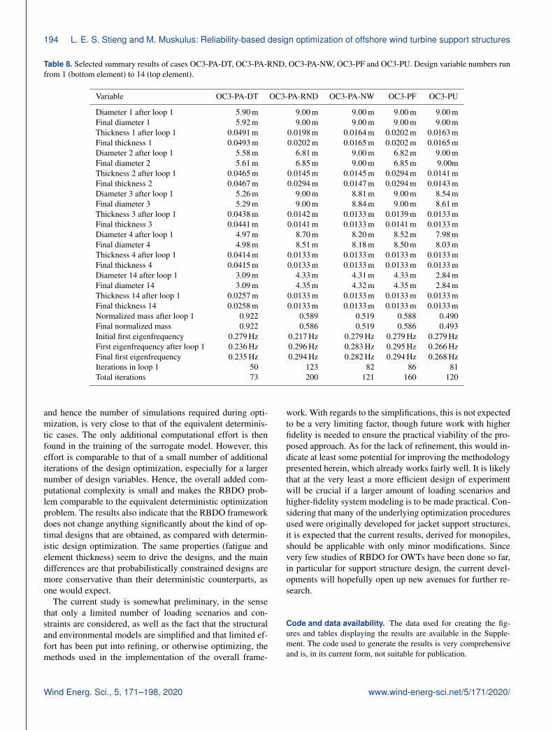
194 L. E. S. Stieng and M. Muskulus: Reliability-based design optimization of offshore wind turbine support structures
Table 8. Selected summary results of cases OC3-PA-DT, OC3-PA-RND, OC3-PA-NW, OC3-PF and OC3-PU. Design variable numbers runfrom 1 (bottom element) to 14 (top element).
Variable OC3-PA-DT OC3-PA-RND OC3-PA-NW OC3-PF OC3-PU
Diameter 1 after loop 1 5.90 m 9.00 m 9.00 m 9.00 m 9.00 mFinal diameter 1 5.92 m 9.00 m 9.00 m 9.00 m 9.00 mThickness 1 after loop 1 0.0491 m 0.0198 m 0.0164 m 0.0202 m 0.0163 mFinal thickness 1 0.0493 m 0.0202 m 0.0165 m 0.0202 m 0.0165 mDiameter 2 after loop 1 5.58 m 6.81 m 9.00 m 6.82 m 9.00 mFinal diameter 2 5.61 m 6.85 m 9.00 m 6.85 m 9.00mThickness 2 after loop 1 0.0465 m 0.0145 m 0.0145 m 0.0294 m 0.0141 mFinal thickness 2 0.0467 m 0.0294 m 0.0147 m 0.0294 m 0.0143 mDiameter 3 after loop 1 5.26 m 9.00 m 8.81 m 9.00 m 8.54 mFinal diameter 3 5.29 m 9.00 m 8.84 m 9.00 m 8.61 mThickness 3 after loop 1 0.0438 m 0.0142 m 0.0133 m 0.0139 m 0.0133 mFinal thickness 3 0.0441 m 0.0141 m 0.0133 m 0.0141 m 0.0133 mDiameter 4 after loop 1 4.97 m 8.70 m 8.20 m 8.52 m 7.98 mFinal diameter 4 4.98 m 8.51 m 8.18 m 8.50 m 8.03 mThickness 4 after loop 1 0.0414 m 0.0133 m 0.0133 m 0.0133 m 0.0133 mFinal thickness 4 0.0415 m 0.0133 m 0.0133 m 0.0133 m 0.0133 mDiameter 14 after loop 1 3.09 m 4.33 m 4.31 m 4.33 m 2.84 mFinal diameter 14 3.09 m 4.35 m 4.32 m 4.35 m 2.84 mThickness 14 after loop 1 0.0257 m 0.0133 m 0.0133 m 0.0133 m 0.0133 mFinal thickness 14 0.0258 m 0.0133 m 0.0133 m 0.0133 m 0.0133 mNormalized mass after loop 1 0.922 0.589 0.519 0.588 0.490Final normalized mass 0.922 0.586 0.519 0.586 0.493Initial first eigenfrequency 0.279 Hz 0.217 Hz 0.279 Hz 0.279 Hz 0.279 HzFirst eigenfrequency after loop 1 0.236 Hz 0.296 Hz 0.283 Hz 0.295 Hz 0.266 HzFinal first eigenfrequency 0.235 Hz 0.294 Hz 0.282 Hz 0.294 Hz 0.268 HzIterations in loop 1 50 123 82 86 81Total iterations 73 200 121 160 120
and hence the number of simulations required during opti-mization, is very close to that of the equivalent determinis-tic cases. The only additional computational effort is thenfound in the training of the surrogate model. However, thiseffort is comparable to that of a small number of additionaliterations of the design optimization, especially for a largernumber of design variables. Hence, the overall added com-putational complexity is small and makes the RBDO prob-lem comparable to the equivalent deterministic optimizationproblem. The results also indicate that the RBDO frameworkdoes not change anything significantly about the kind of op-timal designs that are obtained, as compared with determin-istic design optimization. The same properties (fatigue andelement thickness) seem to drive the designs, and the maindifferences are that probabilistically constrained designs aremore conservative than their deterministic counterparts, asone would expect.
The current study is somewhat preliminary, in the sensethat only a limited number of loading scenarios and con-straints are considered, as well as the fact that the structuraland environmental models are simplified and that limited ef-fort has been put into refining, or otherwise optimizing, themethods used in the implementation of the overall frame-
work. With regards to the simplifications, this is not expectedto be a very limiting factor, though future work with higherfidelity is needed to ensure the practical viability of the pro-posed approach. As for the lack of refinement, this would in-dicate at least some potential for improving the methodologypresented herein, which already works fairly well. It is likelythat at the very least a more efficient design of experimentwill be crucial if a larger amount of loading scenarios andhigher-fidelity system modeling is to be made practical. Con-sidering that many of the underlying optimization proceduresused were originally developed for jacket support structures,it is expected that the current results, derived for monopiles,should be applicable with only minor modifications. Sincevery few studies of RBDO for OWTs have been done so far,in particular for support structure design, the current devel-opments will hopefully open up new avenues for further re-search.
Code and data availability. The data used for creating the fig-ures and tables displaying the results are available in the Supple-ment. The code used to generate the results is very comprehensiveand is, in its current form, not suitable for publication.
Wind Energ. Sci., 5, 171–198, 2020 www.wind-energ-sci.net/5/171/2020/

L. E. S. Stieng and M. Muskulus: Reliability-based design optimization of offshore wind turbine support structures 195
Supplement. The supplement related to this article is availableonline at: https://doi.org/10.5194/wes-5-171-2020-supplement.
Author contributions. LESS formulated the main idea and im-plemented the method, conducted the analysis, created the figuresand wrote the manuscript. MM provided essential input and sugges-tions throughout the process, aided in the formulation of the scopeof the work and helped with the composition of the manuscript.
Competing interests. The authors declare that they have no con-flict of interest.
Acknowledgements. This work has been partly supported byNOWITECH FME (Research Council of Norway, contract no.193823) and by the Danish Council for Strategic Research throughthe project “Advancing BeYond Shallow waterS (ABYSS) – Opti-mal design of offshore wind turbine support structures”.
Financial support. This research has been supported by theNorges Forskningsråd (grant no. 193823) and the StrategiskeForskningsråd (grant no. 1305-00020B).
Review statement. This paper was edited by Athanasios Koliosand reviewed by two anonymous referees.
References
Abdallah, I., Lataniotis, C., and Sudret, B.: Parametric hierarchicalkriging for multi-fidelity aero-servo-elastic simulators – Applica-tion to extreme loads on wind turbines, Probabilist. Eng. Mech.,55, 67–77, 2019.
Andersen, L., Vahdatirad, M., Sichani, M., and Sørensen, J.: Naturalfrequencies of wind turbines on monopile foundations in clayeysoils – A probabilistic approach, Comput. Geotech., 43, 1–11,2012.
Aoues, Y. and Chateauneuf, A.: Benchmark study of numericalmethods for reliability-based design optimization, Struct. Mul-tidiscip. O., 41, 277–294, 2010.
Ben-Tal, A., Ghaoui, L. E., and Nemirovski, A.: Robust Optimiza-tion, Princeton University Press, New Jersey, USA, 2009.
Brochu, E., Cora, V. M., and de Freitas, N.: A Tutorial on BayesianOptimization of Expensive Cost Functions, with Application toActive User Modeling and Hierarchical Reinforcement Learn-ing, available at: https://arxiv.org/abs/1012.2599 (last access:18 July 2019), 2010.
Caboni, M., Minisci, E., and Riccardi, A.: Aerodynamic De-sign Optimization of Wind Turbine Airfoils under Aleatoryand Epistemic Uncertainty, J. Phys. Conf. Ser., 1037, 042011,https://doi.org/10.1088/1742-6596/1037/4/042011, 2018.
Carswell, W., Arwade, S. R., DeGroot, D. J., and Lackner, M. A.:Soil–structure reliability of offshore wind turbine monopile foun-dations, Wind Energy, 18, 483–498, 2015.
Chen, C. and Duffour, P.: Modelling damping sources in monopile-supported offshore wind turbines, Wind Energy, 21, 1121–1140,2018.
Chen, X., Hasselman, T., and Neill, D.: Reliability based structuraldesign optimization for practical applications, in: Proceedingsof the 38th AIAA structures, structural dynamics, and materialsconference, AIAA, Florida, USA, 1997.
Chew, K.-H., Tai, K., Ng, E. Y. K., and Muskulus, M.: Analyticalgradient-based optimization of offshore wind turbine substruc-tures under fatigue and extreme loads, Mar. Struct., 47, 23–41,2016.
Choi, S.-K., Grandhi, R. V., and Canfield, R. A.: Reliability-basedStructural Design, Springer-Verlag, London, UK, 2007.
Couceiro, I., París, J., Navarrina, F., Guizán, R., and Colominas,I.: Optimization of Offshore Steel Jackets: Review and Pro-posal of a New Formulation for Time-Dependent Constraints,Arch. Comput. Method. E., https://doi.org/10.1007/s11831-019-09342-y, online first, 2019.
Damgaard, M., Andersen, L., Ibsen, L., Toft, H., and Sørensen, J.: Aprobabilistic analysis of the dynamic response of monopile foun-dations: Soil variability and its consequences, Probabilist. Eng.Mech., 41, 46–59, 2015.
Depina, I., Le, T. M. H., Fenton, G., and Eiksund, G.: Reliabilityanalysis with Metamodel Line Sampling, Struct. Saf., 60, 1–15,2016.
Depina, I., Papaioannou, I., Straub, D., and Eiksund, G.: Cou-pling the cross-entropy with the line sampling method for risk-based design optimization, Struct. Multidiscip. O., 55, 1589–1612, 2017.
Det Norske Veritas: Design of Offshore Wind Turbine Structures,Offshore Standard, DNV-OS-J101, DNV-GL, Høvik, Norway,2016.
Dimitrov, N. K.: Structural Reliability of Wind Turbine Blades, PhDthesis, Technical University of Denmark, 2013.
Dong, W., Moan, T., and Gao, Z.: Fatigue reliability analysis of thejacket support structure for offshore wind turbine considering theeffect of corrosion and inspection, Reliability Engineering andSystem Safety, 106, 11–27, 2012.
Du, X. and Chen, W.: Sequential Optimization and Reliability As-sessment Method for Efficient Probabilistic Design, J. Mech. De-sign, 126, 225–233, 2004.
Dubourg, V.: Adaptive surrogate models for reliability analysis andreliability-based design optimization, PhD thesis, Blaise PascalUniversity, Claremont-Ferrand, France, 2011.
Enevoldsen, I. and Sørensen, J.: Reliability-based optimization instructural engineering, Struct. Saf., 15, 169–196, 1994.
Fedem Technology: Fedem User’s Guide, release 7.2.1, FedemTechnology AS, Trondheim, Norway, 2016.
Fischer, T., de Vries, W., and Schmidt, B.: Upwind Design Basis,Technical Report, Endowed Chair of Wind Energy (SWE) at theInstitute of Aircraft Design, Stuttgart University, 2010.
Frangopol, D. M. and Maute, K.: Reliability-Based Optimization ofCivil and Aerospace Structural Systems, in: Engineering DesignReliability Handbook, edited by: Nikolaidis, E., Ghiocel, D. M.,and Singhal, S., CRC Press, Boca Raton, USA, 2005.
Häfele, J., Gebhardt, C. G., and Rolfes, R.: A compari-son study on jacket substructures for offshore wind tur-bines based on optimization, Wind Energ. Sci., 4, 23–40,https://doi.org/10.5194/wes-4-23-2019, 2019.
www.wind-energ-sci.net/5/171/2020/ Wind Energ. Sci., 5, 171–198, 2020

196 L. E. S. Stieng and M. Muskulus: Reliability-based design optimization of offshore wind turbine support structures
Haj, A.-K. E., Soubra, A.-H., and Fajoui, J.: Probabilistic analysisof an offshore monopile foundation taking into account the soilspatial variability, Comput. Geotech., 106, 205–216, 2019.
Hu, W.: Reliability-Based Design Optimization of Wind TurbineSystems, in: Advanced Wind Turbine Technology, edited by: Hu,W., Springer International Publishing AG, Cham, Switzerland,2018.
Hu, W., Choi, K. K., and Cho, H.: Reliability-based design opti-mization of wind turbine blades for fatigue life under dynamicwind load uncertainty, Struct. Multidiscip. O., 54, 953–970,2016.
Hübler, C. J.: Efficient probabilistic analysis of offshore wind tur-bines based on time-domain simulations, PhD thesis, LeibnizUniversität Hannover, 2019.
Huchet, Q., Mattrand, C., Beaurepaire, P., Relun, N., and Gayton,N.: AK-DA: An efficient method for the fatigue assessment ofwind turbine structures, Wind Energy, 22, 638–652, 2019.
International Electrotechnical Commission: Wind turbines – Part3: Design requirements for offshore wind turbines, InternationalStandard, IEC 61400-3, IEC, Geneva, Switzerland, 2009.
Jiang, Z., Hu, W., Dong, W., Gao, Z., and Ren, Z.: Structural Relia-bility Analysis of Wind Turbines: A Review, Energies, 10, 2099,https://doi.org/10.3390/en10122099, 2017.
Jin, R., Du, X., and Chen, W.: The use of metamodeling techniquesfor optimization under uncertainty, Struct. Multidiscip. O., 25,99–116, 2003.
Jones, D. R., Schonlau, M., and Welch, W. J.: Efficient Global Op-timization of Expensive Black-Box Functions, J. Global Optim.,13, 455–492, 1998.
Jonkman, J. and Musial, W.: Offshore Code Comparison Collabo-ration (OC3) for IEA Task 23 Offshore Wind Technology andDeployment, Technical Report, NREL/TP-5000-48191, NREL,Golden, USA, 2010.
Jonkman, J., Butterfield, S., Musial, W., and Scott, G.: Definition ofa 5-MW Reference Wind Turbine for Offshore System Develop-ment, Technical Report, NREL/TP-500-38060, NREL, Golden,USA, 2009.
Kallehave, D., Byrne, B. W., Thilsted, C. L., andMikkelsen, K. K.: Optimization of monopiles for off-shore wind turbines, Philos. T. R. Soc. A, 373, 20140100,https://doi.org/10.1098/rsta.2014.0100, 2015.
Kang, B.-S., Park, G.-J., and Arora, J. S.: A review of optimizationof structures subjected to transient loads, Struct. Multidiscip. O.,31, 81–95, 2006.
Karadeniz, H., Togan, V., Daloglu, A., and Vrouwenvelder, T.:Reliability-based optimisation of offshore jacket-type structureswith an integrated-algorithms system, Ships Offshore Struc., 5,67–74, 2010a.
Karadeniz, H., Togan, V., and Vrouwenvelder, T.: Optimizationof Steel Monopod-Offshore-Towers Under Probabilistic Con-straints, Journal of Offshore Mechanics and Artcic Engineering,132, 021605, https://doi.org/10.1115/1.4000401, 2010b.
Kaymaz, I.: Application of kriging method to structural reliabilityproblems, Struct. Saf., 27, 133–151, 2005.
Kim, D. H. and Lee, S. G.: Reliability analysis of offshore windturbine support structures under extreme ocean environmentalloads, Renew. Energ., 79, 161–166, 2015.
Kolios, A. I.: A Multi-Configuration Approach To Reliability BasedStructural Integrity Assessment For Ultimate Strength, PhD the-sis, Cranfield University, Cranfield, UK, 2010.
Kostandyan, E. E. and Sørensen, J. D.: Reliability Assessment ofSolder Joints in Power Electronic Modules by Crack DamageModel for Wind Turbine Applications, Energies, 4, 2236–2248,2011.
Kreisselmeier, G. and Steinhauser, R.: Systematic Control Designby Optimizing a Vector Performance Index, in: Proceedings ofthe IFAC Symposium on computer Aided Design of Control Sys-tems, IFAC, Zurich, Switzerland, 1979.
Kucherenko, S., Albrecht, D., and Saltelli, A.: Exploring multi-dimensional spaces: a Comparison of Latin Hypercube and QuasiMonte Carlo Sampling Techniques, available at: https://arxiv.org/abs/1505.02350 (last access: 18 July 2019), 2015.
Lee, J.-O., Yang, Y.-S., and Ruy, W.-S.: A comparative studyon reliability-index and target-performance-based probabilisticstructural design optimization, Comput. Struct., 80, 257–269,2002.
Lee, Y.-S., Choi, B.-L., Lee, J. H., Kim, S. Y., and Han, S.:Reliability-based design optimization of monopile transitionpiece for offshore wind turbine system, Renew. Energ., 71, 729–741, 2014.
Leimeister, M. and Kolios, A.: A review of reliability-based meth-ods for risk analysis and their application in the offshore windindustry, Renew. Sust. Energ. Rev., 91, 1065–1076, 2018.
Li, H., Cho, H., Sugiyama, H., Choi, K. K., and Gaul, N. J.:Reliability-based design optimization of wind turbine drivetrainwith integrated multibody gear dynamics simulation consider-ing wind load uncertainty, Struct. Multidiscip. O., 56, 183–201,2017.
Márquez-Domínguez, S. and Sørensen, J. D.: Fatigue Reliabilityand Calibration of Fatigue Design Factors for Offshore WindTurbines, Energies, 5, 1816–1834, 2012.
Marsland, S.: Machine Learning – An Algorithmic Perspective, 2ndEdn., CRC Press, Florida, USA, 2015.
Melchers, R.: Structural reliability: analysis and prediction, Wiley,New York, USA, 1999.
Mockus, J.: On the Bayes Methods for Seeking the Extremal Point,in: Proceedings of the 6th IFAC World Congress, IFAC, Boston,USA, 1975.
Morató, A., Sriramula, S., and Krishnan, N.: Kriging models foraero-elastic simulations and reliability analysis of offshore windturbine support structures, Ships Offshore Struc., 14, 545–558,2019.
Müller, K. and Cheng, P. W.: Application of a MonteCarlo procedure for probabilistic fatigue design of float-ing offshore wind turbines, Wind Energ. Sci., 3, 149–162,https://doi.org/10.5194/wes-3-149-2018, 2018.
Negm, H. M. and Maalawi, K. Y.: Structural design optimization ofwind turbine towers, Comput. Struct., 74, 649–666, 2000.
Nocedal, J. and Wright, S. J.: Numerical Optimization, 2nd Edn.,Springer, New York, 2006.
Oest, J., Sørensen, R., Overgaard, L. C. T., and Lund, E.: Structuraloptimization with fatigue and ultimate limit constraints of jacketstructures for large offshore wind turbines, Struct. Multidiscip.O., 55, 779–793, 2017.
Wind Energ. Sci., 5, 171–198, 2020 www.wind-energ-sci.net/5/171/2020/

L. E. S. Stieng and M. Muskulus: Reliability-based design optimization of offshore wind turbine support structures 197
Oest, J., Sandal, K., Schafhirt, S., Stieng, L. E. S., and Muskulus,M.: On gradient-based optimization of jacket structures for off-shore wind turbines, Wind Energy, 21, 953–967, 2018.
Press, W. H., Teukolsky, S. A., Vetterling, W. T., and Flannery, B. P.:Numerical Recipes: The Art of Scientific Computing, 3rd Edn.,Cambridge University Press, New York, 2007.
Rafsanjani, H. M., Sørensen, J. D., Fæster, S., and Sturlason, A.:Fatigue Reliability Analysis of Wind Turbine Cast Components,Energies, 10, 466, https://doi.org/10.3390/en10040466, 2017.
Rasmussen, C. E. and Williams, C. K. I.: Gaussian Processes forMachine Learning, MIT Press, Massachussets, USA, 2006.
Ronold, K. O., Wedel-Heinen, J., and Christensen, C. J.: Reliability-based fatigue design of wind-turbine rotor blades, Eng. Struct.,21, 1101–1114, 1999.
Rosenblatt, M.: Remarks on a Multivariate Transformation, Ann.Math. Stat., 23, 470–472, 1952.
Rychlik, I.: A new definition of the rainflow cycle counting method,Int. J. Fatigue, 9, 119–121, 1987.
Sandal, K., Verbart, A., and Stolpe, M.: Conceptual jacket designby structural optimization, Wind Energy, 21, 1423–1434, 2018.
Santner, T. J., Williams, B. J., and Notz, W. I.: The Design and Anal-ysis of Computer Experiments, 2nd Edn., Springer, New York,USA, 2018.
Sørensen, J., Frandsen, S., and Tarp-Johansen, N.: Effective turbu-lence models and fatigue reliability in wind farms, Probabilist.Eng. Mech., 23, 531–538, 2008.
Sørensen, J. D. and Tarp-Johansen, N. J.: Reliability-based Opti-mization and Optimal Reliability Level of Offshore Wind Tur-bines, Int. J. Offshore Polar, 15, 141–146, 2005.
Sørensen, J. D. and Toft, H. S.: Probabilistic Design of Wind Tur-bines, Energies, 3, 241–257, 2010.
Standards Norway: Design of steel structures, Rev. 3, February2013, NORSOK Standard N-004, Standards Norway, Lysaker,Norway, 2013.
Stieng, L. E. S. and Muskulus, M.: Reducing the numberof load cases for fatigue damage assessment of offshorewind turbine support structures using a simple severity-based sampling method, Wind Energ. Sci., 3, 805–818,https://doi.org/10.5194/wes-3-805-2018, 2018.
Stieng, L. E. S. and Muskulus, M.: Load case reduction for offshorewind turbine support structure fatigue assessment by importancesampling with two-stage filtering, Wind Energy, 22, 1472–1486,https://doi.org/10.1002/we.2382, 2019.
Teixeira, R., O’Connor, A., Nogal, M., Nichols, J., and Spring, M.:Structural probabilistic assessment of Offshore Wind Turbine op-eration fatigue based on Kriging interpolation, in: Proceedings of27th European Safety and Reliability Conference (ESREL 2017),18–22, ESRA, Portoroz, Slovenia, 2017.
Teixeira, R., Nogala, M., O’Connor, A., Nichols, J., and Dumas, A.:Stress-cycle fatigue design with Kriging applied to offshore windturbines, Int. J. Fatigue, 125, 454–467, 2019.
Thöns, S., Faber, M. H., and Rücker, W.: Support Structure Reliabil-ity Of Offshore Wind Turbines Utilizing An Adaptive ResponseSurface Method, in: Proceedings of the ASME 2010 29th Inter-national Conference on Ocean, Offshore and Arctic Engineering,406–416, ASME, Shanghai, China, 2010.
Toft, H. S. and Sørensen, J. D.: Reliability-based design of windturbine blades, Struct. Saf., 33, 333–342, 2011.
Toft, H. S., Svenningsen, L., Moser, W., Sørensen, J. D., andThøgersen, M. L.: Assessment of wind turbine structural in-tegrity using response surface methodology, Eng. Struct., 106,471–483, 2016a.
Toft, H. S., Svenningsen, L., Sørensen, J. D., Moser, W., andThøgersen, M. L.: Uncertainty in wind climate parameters andtheir influence on wind turbine fatigue loads, Renew. Energ., 60,352–361, 2016b.
Tu, J., Choi, K. K., and Park, Y. H.: A New Study on Reliability-Based Design Optimization, J. Mech. Design, 121, 557–564,1999.
Tunga, M. A. and Demiralp, M.: A factorized high dimensionalmodel representation on the nodes of a finite hyperprismatic reg-ular grid, Appl. Math. Comput., 164, 865–883, 2005.
Uys, P. E., Farkas, J., Jármai, K., and van Tonder, F.: Optimisationof a steel tower for a wind turbine structure, Eng. Struct., 29,1337–1342, 2007.
Valdebenito, M. A. and Schuëller, G. I.: A survey on approaches forreliability-based optimization, Struct. Multidiscip. O., 42, 645–663, 2010a.
Valdebenito, M. A. and Schuëller, G. I.: A survey on approaches forreliability-based optimization, Struct. Multidiscip. O., 42, 645–663, 2010b.
Velarde, J., Kramhøft, K., and Sørensen, J. D.: Reliability-basedDesign Optimization of Offshore Wind Turbine Concrete Struc-tures, in: Proceedings of the 13th International Conference onApplications of Statistics and Probability in Civil Engineering,ICASP13, International Civil Engineering Risk and ReliabilityAssociation, Seoul, South Korea, 2019.
Veldkamp, D.: A Probabilistic Evaluation of Wind Turbine FatigueDesign Rules, Wind Energy, 11, 655–672, 2008.
Wandji, W. N., Natarajan, A., and Dimitrov, N.: Development anddesign of a semi-floater substructure for multi-megawatt windturbines at 50+m water depths, Ocean Eng., 125, 226–237,2016.
Wang, G. G. and Shan, S.: Review of Metamodeling Techniques inSupport of Engineering Design Optimization, J. Mech. Design,129, 370–380, 2006.
Wei, K., Arwade, S. R., and Myers, A. T.: Incremental wind-waveanalysis of the structural capacity of offshore wind turbine sup-port structures under extreme loading, Eng. Struct., 79, 58–69,2014.
Yang, H. and Zhu, Y.: Robust design optimization of supportingstructure of offshore wind turbine, J. Mar. Sci. Technol., 20, 689–702, 2015.
Yang, H., Zhu, Y., Lu, Q., and Zhang, J.: Dynamic reliability baseddesign optimization of the tripod sub-structure of offshore windturbines, Renew. Energ., 78, 16–25, 2015.
Yang, H., Zhang, X., and Xiao, F.: Dynamic Reliability based De-sign Optimization of Offshore Wind Turbines Considering Un-certainties, in: Proceedings of the Thirteenth (2018) Pacific-AsiaOffshore Mechanics Symposium, 325–331, The InternationalSociety of Offshore and Polar Engineers, Jeju, South Korea,2018.
Yeter, B., Garbatov, Y., and Soares, C. G.: Reliability Of OffshoreWind Turbine Support Structures Subjected To Extreme Wave-Induced Loads And Defects, in: Proceedings of the ASME 201635th International Conference on Ocean, Offshore and Arctic En-gineering, V003T02A060, ASME, Busan, South Korea, 2016.
www.wind-energ-sci.net/5/171/2020/ Wind Energ. Sci., 5, 171–198, 2020

198 L. E. S. Stieng and M. Muskulus: Reliability-based design optimization of offshore wind turbine support structures
Yoon, G. L., Kim, S. B., and Kim, H. Y.: Reliability Analysis ofMonopile for Offshore Wind Foundation Using the ResponseSurface Method, in: New Frontiers of Geotechnical EngineeringGSP 423, 108–117, American Society of Civil Engineers, Shang-hai, China, 2014.
Yoshida, S.: Wind Turbine Tower Optimization Method Using a Ge-netic Algorithm, Wind Engineering, 30, 453–469, 2006.
Youn, B. D. and Choi, K. K.: An Investigation of Nonlinearityof Reliability-Based Design Optimization Approaches, J. Mech.Design, 126, 403–411, 2003.
Youn, B. D., Choi, K. K., and Park, Y. H.: Hybrid Analysis Methodfor Reliability-Based Design Optimization, J. Mech. Design,125, 221–232, 2003.
Zang, C., Friswell, M., and Mottershead, J.: A review of robust opti-mal design and its application in dynamics, Comput. Struct., 83,315–326, 2005.
Zwick, D., Muskulus, M., and Moe, G.: Iterative Optimization Ap-proach for the Design of Full-Height Lattice Towers for OffshoreWind Turbines, Enrgy. Proced., 24, 297–304, 2012.
Wind Energ. Sci., 5, 171–198, 2020 www.wind-energ-sci.net/5/171/2020/