structural reliability approach to strain based design of offshore pipelines

Structural Reliability Approach to Strain Based Design of Offshore Pipelines W. Cimbali, F. Marchesani, D. Zenobi

Field Upstream Facilities and Pipeline Division, Snamprogetti Fano, Italy

ABSTRACT High longitudinal strains on the pipeline may be activated by sharp bent configurations during the different lifetime phases. A strain based design may be, in these cases, applied given that the pipe is predominantly loaded in global displacement control. The failure is related to the ductile tearing of the defective girth welds: the maximum allowable longitudinal strain is identified by guaranteeing the pipeline integrity with respect to this limit state. The applications of deterministic fracture mechanics assessment procedures to the predictions of fitness for purpose requires the use of data that are often subject to considerable uncertainty. The extreme bounding values for the relevant parameters can lead, in some circumstances, to unacceptably over-conservative predictions of structural integrity. An alternative approach is to use structural reliability methods to allow for the uncertainties in the parameters and to assess the probability of failure of structures containing flaws. A probabilistic fracture mechanics analyses is carried out according to the assessment procedures described by British Standards codes (BS7910, 1999) and using a statistical simulation method (Monte Carlo) for solving the limit state equation. The uncertainties (i.e., specific statistical distributions) of the following parameters are taken into account, expected to most affect the evaluation of the pipe criticality in the high strain conditions: applied longitudinal strains, strength of the base material, strength of the weld metal, CTOD, flaw size. The acceptable probability of failure depends on the consequences of failure for the structure; for the offshore pipeline reference is made to the standard OS-F101 (DNV 2000). This approach avoids the use of “all purpose” safety factors for ECA evaluations and allows to optimise the final pipeline configuration on the seabed in high strain conditions and to considerably reduce the amounts of the intervention works still keeping the appropriate level of safety. KEY WORDS: Offshore Pipelines; Structural Reliability; Displacement Controlled Condition; Engineering Criticality Assessment; Ultimate Limit State; Probability Density Function; Cumulative Probability Function; Failure Assessment Domain; Crack Tip Opening Displacement.

INTRODUCTION The use of the “strain based” design criterion in offshore pipeline tecnology has widely increased in the last years since a general consensus has been developed about the fact that, in many circumstances, it is more valid than a “stress based” design criterion. This scenario is justified by the current experiences on the engineering projects, where the application of a “stress based” design criterion often requires demanding measures while safe and economically attractive solutions are generated by the rational application of a “strain based” criterion. International codes and regulations clearly state that the “strain based” design criterion is applicable only at displacement controlled conditions (DCC), to be identified as the system conditions in which the structural response is primarily governed by imposed geometric displacements (DNV 2000): as a consequence the strains, once activated by the external loads, are however controlled by the external boundaries. In these cases failure occurs at deformation level which activate material (ductile tearing, cracking, etc.) or shape (ovalization, wrinkling and/or bulging, etc.) instabilities. The design equation for the “strain based” design criterion is related to the check of the applied strains (εapp) with respect to the permissible strains (εall) and can be expressed as: (εapp) ≤ (εall) (1) The strain component to be verified in this general equation is the total longitudinal strain, generated by the combined axial force and bending, which excessive development may cause the pipeline failure. This damage, which consequences could be the release of the transported fluid into the external environment and/or the line flooding, may be considered an ultimate limit state (ULS) for an offshore pipeline. Main modes related to this ULS condition are fracture/plastic collapse of the circumferential weld, joint ovalisation and local buckling of the steel cylindrical walls: this paper deals only with the first one and describes a complete (Level 3) probabilistic approach to the engineering criticality assessment (ECA) equations in order to take into account most of the system uncertainties and reach an important twofold aim for the pipeline, i.e. to satisfy the required safety levels and contemporary minimise any design conservatism.

9

Proceedings of The Twelfth (2002) International Offshore and Polar Engineering ConferenceKitakyushu, Japan, May 26–31, 2002Copyright © 2002 by The International Society of Offshore and Polar EngineersISBN 1-880653-58-3 (Set); ISSN 1098-6189 (Set)

MAIN SCENARIOS FOR DCC In general, the occurrence of the weld collapse failure mode is related to the high concentration of bending strains generated by the fixed geometry of the external boundaries. A typical situation is during pipelay, for a pipe bent on the fixed ramp of a lay barge to allow it to achieve the desirable slope at the exit. For a certain combination of parameters such as applied lay pull, submerged weight, bending stiffness and water depth, the pipe will be smoothly bent by the sequence of rollers located along the stinger so that an evenly distributed contact reaction is responsible for pipe bending. This condition is considered as displacement controlled since the pipe curvature cannot exceed the curvature defined by the contact points at the rollers. However, in some circumstances, the applied lay pull might not be sufficient to keep the pipeline in a condition of continuous contact with the fixed stinger, thus causing the pipeline lift off the stinger between the first and the last roller. In other words, the pipe bending on the stinger is bounded in one direction and, therefore, the condition can be defined as displacement controlled only for a combination of parameters which ensures that the pipeline will remain in an even contact with the stinger rollers under the applied load conditions. This issue, which mainly relates to “S” lay technology, is still applicable for “Reel” or “J” lay technologies in conditions where the load variations do not affect the strain values. Local concentration of bending strains are also often related to an offshore pipeline laid on a seabed profile characterised by undulations, due to the fact that the pipe will try to conform with the seabottom unevenness. For a certain combination of parameters such as residual lay pull (depending on water depth and lay criteria on overbend), submerged weight and bending stiffness, the pipe will be able to conform with these undulations. In these conditions the maximum achievable bending is controlled by the nat ural profile of the seabed, giving therefore a typical DCC. Large bending strains may be also generated on the pipeline when expanding at the action of the high pressure and temperature loads. If the line is not free to expand, e.g. restrained by soil friction, it will be subjected to an axial compressive load. In these cases it is possible to consider the pipeline in DCC if either buried with cover preventing thermal expansion or resting on the seabed, where it could recover the thermal expansion by buckling on the horizontal plane when compressive load reaches a critical value. FRACTURE/PLASTIC COLLAPSE OF A DEFECTIVE GIRTH WELD In typical DCC, where the pipeline is subjected to sharp bent configurations and the applied strains widely overcome the elastic limit, high stress levels are activated at the circumferential welds. As a consequence an ECA of the defective girth weld is required in order to evaluate which is the limit external condition applicable without causing any weld criticality. Minimum toughness requirements currently applied in specifications for girth welds should exclude the brittle fracture at a defect for stress levels lower than yielding: therefore failure starting at a defective girth weld can be classified as plastic collapse. Bein g this the scenario, the criticality is significantly affected by the differences between weld and pipe material hardening behaviours: particular importance is to be given to the matching ratio (MR), which is defined by the following expression:

BMY

AWYMR

σσ

= , (2)

where AWYσ = yield stress of all weld metal,

BMYσ = yield stress of the base material.

Fig. 1 shows possible combinations of matching conditions and the relevant effects in absence of flaws.

Basic weld metal - base metal combinations Combination Sequence of phenomena Type

A YW<TW<YB <TB Undermatching B YW<YB <TW<TB Undermatching C YW<YB <TB <TW Undermatching D YB <TB <YW<TW Overrnatching E YB <YW<TB<TW Overmatching F YB <YW<TW<TB Overmatching

Figure 1 – Basic weld metal (W) - base metal (B) combinations (Y = yeld stress, T = ultimate tensile stress) The general effect of strength mismatch in flaw free transverse butt welds, if the loading exceeds that necessary to cause yielding in whichever is the lower strength material, is to concentrate plastic strains into that material. If the loading does not reach this level, the only effect of the strength mismatch is the level of residual stress present. The presence of flaws in the joint complicates this situation and can therefore alter the extent to which mismatch effects are apparent: nevertheless it has been widely agreed (BS7910,1999 and Denys, 1994) that an over-matching weld metal strength (MR > 1) can protect the crack plane against net section yielding. The gross section yielding is, actually, always preferred since, in this situation, any plastification mainly develop into the parent pipe. A major concern of the pipeline “strain based” verification is the transformation of the “weld” critical stresses into the “pipe” critical strains. The applied stresses are dictated by the strains applied to the base pipe and the base pipe material, as welds usually have negligible longitudinal lengths with respect to the pipe diameter; on the other hand, fracture and collapse behaviour is governed by the mechanical properties of the material surrounding the defect: consequently, the fracture toughness of the weld metal is used for the ECA. The failure assessment demain (FAD) might be determined using the weld metal strengths: however, according to the fact that the applied stresses are better related to the parent pipe behaviour, the pipe material is usually preferred to determine the FAD relevant to the weld metal too. Plastic collapse equations are usually according to the Kastner's formulation, but alternative equations may also be used (Clyne,1995). Nevertheless, the general procedure for the probabilistic approach, remains still applicable. The application of deterministic fracture mechanics assessment procedures to the predictions of fitness for purpose requires the use of data that are often subject to considerable uncertainty. The extreme bounding values for the relevant parameters can lead, in some

10

circumstances, to unacceptably over-conservative predictions of structural integrity. An alternative approach is to use structural reliability methods to allow for the uncertainties in the parameters and to assess the probability of failure of structures containing flaws. The reference code supplies the application of the safety factors reported in Tab.1: their application to the relevant input quantities in a deterministic assessment of structural integrity should provide a means of relating the deterministic analysis to a specific (target) failure probability. In most of the engineering projects and design activities, the applications of these safety factors either to the “characteristic values” or to the “mean values” of the relevant design parameters, have generated unacceptable over-conservative predictions of structural integrity. In installation, latent conservative factors could be recognised in the usual approach to keep the allowable strain within 0.3% (static settings), in order to be assured against the fracture/plastic collapse failure mode of the large number of joints called to experience the same applied value (system effect). In addition, where the approach for installation is to assume the 0.3% allowable strain in order to evaluate the related limit flaw size, the safety factors on the CTOD (crack tip opening displacement) are often disregarded. Other typical examples are those of pipelines in operating conditions, which specific ECA of the defected girth weld would define an allowable situation more severe than the one due to the local buckling failure mode based on load controlled condition. In this case, the “strain based” design criterion would be completely nullified by this semi-probabilistic approach to the weld since the allowable strain would remain close to or slightly above the elastic values. The partial safety factors of Tab. 1 are derived for a load controlled condition and making certain assumptions about the variables and their statistical distributions: however they can be considered inappropriate to most of the offshore pipeline situations in DCC. The alternative is, consequently, to carry out a probabilistic fracture mechanics analysis, based on Level 3 assessment: it can be conducted by using the Monte Carlo simulation and taking special care to ensure that the statistical distributions employed are derived from data representative of the materials and conditions of the pipeline to be assessed. Table 1 – Recommended partial factors for different target probabilities

of failure (BS7910) p(F) = 2.3 X 10-1 10-3 7 X 10-5 10-5

βt = 0.739 3.09 3.8 4.27 Stress, σ (COV)σ γσ γσ γσ γσ 0.1 1.05 1.2 1.25 1.3 0.2 1.1 1.25 1.35 1.4 0.3 1.12 1.4 1.5 1.6 Flaw size, α (COV)α γα γα γα γα 0.1 1.0 1.4 1.5 1.7 0.2 1.05 1.45 1.55 1.8 0.3 1.08 1.5 1.65 1.9 0 5 1.15 1.7 1.85 2.1 Toughness, k (COV)k γk γk γk γk 0.1 1 1.3 1.5 1.7 0.2 1 1.8 2.6 3.2 0.3 1 2.85 NP NP Toughness, δ (COV)δ γδ γδ γδ γδ 0.2 1 1.69 2.25 2.89 0.4 1 3.2 6.75 10 0.6 1 8 NP NP Yield strength (COV)y γy γy γy γy 0.1 1 1.05 1.1 1.2

NOTE 1 γσ, is a multiplier to the mean stress of a normal distribution.

NOTE 2 γα, is a multiplier to the mean flaw height of a normal distribution.

NOTE 3 γk, or γδ are dividers to the mean minus one standard deviation value of fracture toughness of a Weibull distribution.

NOTE 4 γy, is a divider to the mean minus two standard deviation value of yield strength of a log-normal distribution.

NOTE 5 These partial safety factors may not be appropriate for other statistical distributions or coefficients of variation (COV).

PROBABILISTIC LIMIT STATE APPROACH Different statistical levels may be used for the probabilistic approach to the ECA of the defected girth weld: the higher is the level and, both, the more precise are the required information on the statistics of the analysis parameters and the more accurate are the required analysis methods. On the other hand, the promising aspect is that the higher is the statistical level and the lower will be the level of conservatism for the same required target probability. Level 1 is the simplest level, alternatively called “semiprobabilistic”, since the limit state equation is still resolved in deterministic manner. Calibrated partial safety factors are defined for each analyses parameters and are applied to the relevant “characteristic values”, in order to take into account the possible physic uncertainties (input loads, system geometries and resistances), statistical uncertainties and structural model uncertainties. For fracture/plastic collapse of a defective girth weld, equation (1) may be specified as follows in terms of the total longitudinal stress at the weld critical point:

( ) ( )RWR

REStotlongjj

Pii

APPtotlong XLX γσγγσ /, ,, ≤ (3)

where

REStotlong ,σ resistance (weld strength against tearing),

APPtotlong ,σ stress load (total longitudinal stress applied to the defective

weld, including axial force and bending),

iP

iX γ, parameters for both pipeline geometry and material, and

related partial safety factors,

jjL γ, applied loads and related partial safety factors,

RWRX γ, parameters for weld strength and related partial safety factors.

The inefficacy of the Level 1 approach has been previously clarified by the discussion about the safety factors proposed by the British Standards (BS7910, 1999): as a consequence at least a Level 2 approach should be required. In Level 2 approach the different analyses parameters are considered as random variables: the solution of the limit state equation requires its linearization in Taylor series expansion around a tentative expansion point. This analytical solution method has been considered not enough accurate to the weld analysis, since the relevant limit state equation is highly not-linear with respect to its variables and the analysis efforts not always guarantee a reliable satisfaction of the required failure probability. The application of a Level 3 statistical approach is consequently recognised as the most appropriate. The overall statistical distributions have been considered for the following main analyses parameters: • Applied longitudinal strains, calculated by the structural analyses

on the seabed profile;

11

• Strength of the Base Material (i.e., Parent Pipe), both yielding and ultimate tensile;

• Strength of the Weld Metal, both yielding and ultimate tensile; • CTOD; • Flaw size. The limit state equation has been solved by means of the Monte Carlo simulation. The total longitudinal stress σlong,tot is considered the limit state variable; as a consequence the following format is obtained for the limit state equation (see Fig. 2):

( ) ( ){ } fAPP

totlongRES

totlong pP =≤− 0,, σσ (4)

where:

( )REStotlong,σ resistance (weld strength against tearing)

( )APPtotlong,σ stress load (longitudinal stress applied to the defective

weld)

fp target probability

Assuming that resistances and loads are two independent random variables, the following expression may be obtained (convolution integral)

( ) ( ) ARARf ddffp

AR

σσσσσσ

⋅= ∫ ∫∞

∞−

≤

∞−

(5a)

or, alternatively

( ) ( ) σσσ dfFp ARf ∫∞

∞−

= (5b)

where:

( )σRf PDF for resistance (stress),

( )σRF PCF (cumulative probability function)

for resistance (stress), ( )σAf PDF for applied stress,

( )σAF PCF for applied stress.

0.E+00

2.E-06

4.E-06

6.E-06

8.E-06

1.E-05

1.E-05

1.E-05

2.E-05

2.E-05

2.E-05

2.E-05

400000 450000 500000 550000 600000 650000 700000

longitudinal stresses ( kPa)

pro

bab

ility

den

sity

0.E+00

1.E-04

2.E-04

3.E-04

4.E-04

5.E-04

6.E-04

7.E-04

8.E-04

9.E-04

1.E-03

1.E-03

cum

ula

tive

pro

bab

ility

"Applied" pdf

fA

"Resistant" pdf

f R

density function of the product

FR.f A

cumulative probability of the product FR .fA(its integration gives the target probability

of the limite state equation)

Figure 2 – General statistical representation of the limit state equation

PROBABILISTIC EVALUATION OF APPLIED LOADS The longitudinal stresses acting on the circumferential weld are the same stresses activated on the steel pipe. They are generated by the section forces due to the elasto-plastic behaviour of the pipeline when deformed according to the boundary geometries, combined with the effects of external pressure, residual lay tension and operational loads (temperature and pressure of the exported fluid). The structural analyses by means of FEM (finite element) programs, which consider non-linear model for the pipe material and the two-dimensional stress-strain relationships (longitudinal and hoop directions), allow to evaluate both the total longitudinal strains and the related total longitudinal stresses for a pipeline in DCC, taking into account the load history. Nevertheless these calculated amounts are affected by the variability of the input parameters. The most meaningful influences are expected coming from the variability of the steel pipe characteristic and from the possible uncertainties on the calculated deformed shape and strains (these last ones depending on the adopted structural model as well as on the measurement/simulation accuracies of the boundary geometries). Due to these uncertainties, the total longitudinal stress related to an applied longitudinal strain becomes a random variable, which distribution has been obtained by taking into account the “normal” statistical distribution of the following two variables: yielding of the pipe material, applied total longitudinal strains. The following procedure is adopted to obtain the statistical distribution of the total longitudinal stress related to an applied total longitudinal strain. The total longitudinal strain, generated by combined axial force and bending, is calculated by means of a finite element structural model. This calculated value is considered as a mean value: as a consequence, assigning a proper coefficient of variation (COV) for this random variable (it is generally high: accepted values are 20%) and given that it may be represented as a “normal” random variable, the relevant statistical distribution may be obtained. The non-linear Ramberg-Osgood expression is used, summarised into the following formulas:

εσ σ

σ= +

−

EA

y

n

11

(6)

where

AE

y=

−0 005 1.

σ (7)

−

−

=

y

t

y

tt

E

E

n

σσ

σ

σε

log

005.0

log

(8)

Symbols have the following meanings: σ, ε point on the Ramberg-Osgood relationship; E Young’s modulus; σy yield stress (at strain of 0.5%); σt ultimate tensile stress; εt ultimate tensile strain. The presence of random variables (yielding stress and applied strains) in this articulated and non-linear relationship requires the use of

12

simulation methods to express the final statistical distribution of the total longitudinal stresses: the Monte Carlo Method is applied, with contemporary casual and independent extractions from the distributions of yielding and applied strains (see Fig.3).

µε = 0.30%

µε = 0.15%

µε = 0.45%

0

50000

100000

150000

200000

250000

300000

350000

400000

450000

500000

0 0.05 0.1 0.15 0.2 0.25 0.3 0.35 0.4 0.45 0.5 0.55 0.6 0.65 0.7 0.75

longitudinal strain (%)

str

es

s (

kP

a)

0

2

4

6

8

10

12

14

pro

bab

ilit

y d

ensi

ty

Ramberg-Osgood relationship for X65(calculated on 'minimum' values)

'normal' pdf for applied total longitudinalstrain of 0.30% 'mean' value



Figure 3 – Arrangment of applied strain PDF’s with respect to stress-

strain relationship The following values have been assigned as constant during the application of the Ramberg-Osgood relationship: yielding over tensile stress ratio (usually taken as 0.85); strain at the ultimate stress (usually taken as 10%). The final sample of the total longitudinal stress has, generally, a not symmetric distribution, even if “normal” probability density functions (PDF) have been used for the input random variables: this follows from the trend of the Ramberg-Osgood relationship. Actually, in the central part of the curve, representing the zone of material yielding, the non-linear trend amplifies the dispersion and the asymmetry of the stress sample given by a “normal” strain sample. This effect is reduced when the value of the applied total longitudinal strain is far from the yielding area, where the uniaxial material relationship becomes perfectly (elastic behaviour) or almost (hardening) “linear” (see Figs. 4, 5). According to this aspect, the sample of the total longitudinal stresses may not be simply fitted by means of the two moments method (i.e., “normal” PDF which equals mean and std dev of the sample). A “best fitting” procedure has been applied in order to find a “normal” PDF which can represent the sample of the applied total longitudinal stress resulting from the Monte Carlo simulation.

long. strain=0.44%, stress=446000 kPa

300000.000

350000.000

400000.000

450000.000

500000.000

550000.000

0.100 0.200 0.300 0.400 0.500 0.600 0.700 0.800 0.900 1.000

longitudinal strain (%)

lon

git

ud

inal

str

ess

(kP

a)

mean values of the stress samples obtained by applying theMonte Carlo method to the statistical distributions of theapplied strains

uniaxial Ramberg-Osgood stress-strain relationship for anX65 steel grade

mean value of 0.44% for applied long. Strain PDF: mean value of 483350 kPa for the obtained PDF of applied long.

Stress

Figure 4 – Stress-strain relationship expressed by means of “mean”

values

0

0.000005

0.00001

0.000015

0.00002

0.000025

0.00003

0.000035

0.00004

0.000045

0.00005

40000 90000 140000 190000 240000 290000 340000 390000 440000 490000 540000

total longitudinal stress (kPa)

freq

uen

ces

for

calc

ula

ted

str

ess

sam

ple

sample of applied total longitudinal stress obtained byapplying the Monte Carlo to the longiudinal strain PDF - strainmean value of 0.4%



Figure 5 – Longitudinal stress samples after Monte Carlo applied to

longitudinal strain samples PROBABILISTIC EVALUATION OF THE RESISTANCES The presence of random variables (yield stress σy , ultimate tensile stress σt , CTOD, at Figs. 6,7 and Tab.2, and flaw size) in the articulated and non-linear relationships of ECA requires the use of simulation methods to evaluate the final statistical distribution of the weld resistance, expressed in terms of total longitudinal stresses. Table 2 – Statistic parameters for steel strengths (base material and all

weld) K value:

3=−σ

µ K

K value: 645.1=

−σ

µ K

σ

COV

MR =

µweld/µparent

Parent Pipe Yield (X65)

450 490.5 0.0275

All Weld Metal (MR = 5%) - Yield

452.25 491.88 540.0 0.0541 1.10


429.3 467.10 513.0 0.0543 1.05

All Weld Metal – Ultimate Tensile

586.25 603.93 625.4 0.0208

Parent Pipe Yield (X70)

480 523.2 0.0275


482.4 524.67 576.0 0.0541 1.10


457.92 498.24 547.2 0.0543 1.05

All Weld Metal – Ultimate Tensile

624.94 643.80 666.7 0.0208

NOTES: µ = mean value σ = standar deviation K = characteristic value at assigned fractile COV = σ/µ

13

0

0.005

0.01

0.015

0.02

0.025

0.03

0.035

0.04

420 470 520 570 620 670 720

stress (MPa)

pro

bab

ility

den

sity

X65 -parent pipe yield X65-all weld metal yield (10% ovm)X65-all weld metal yield (5% ovm) X65-all weld metal ultimate tensileX70 -parent pipe yield X70-all weld metal yield (10% ovm)X70-all weld metal yield (5% ovm) X65 - ultimate tensile del parent pipeX70-all weld metal ultimate tensile

Figure 6 – Statistical distributions for base material and weld material

0.0%

10.0%

20.0%

30.0%

40.0%

50.0%

60.0%

70.0%

80.0%

90.0%

100.0%

0.000 0.200 0.400 0.600 0.800 1.000 1.200 1.400 1.600

CTOD (mm)

cum

ula

tive

pro

bil

ity

0.00E+00

2.00E-01

4.00E-01

6.00E-01

8.00E-01

1.00E+00

1.20E+00

1.40E+00

1.60E+00

pro

bab

ilit

y d

ensi

tytest data

data fitting - PCF

3-ParametersWeibull PDF -mean=0.3mm

Figure 7 – Statistical distributions for weld CTOD The Monte Carlo Method is applied, with contemporary casual and independent extractions from the distributions of the statistical parameters. The final sample of the weld resistance (see Fig. 8) has a symmetric distribution, which may be easily represented by means of a “normal” PDF fitted by means of the two moments method. The statistical distributions are affected by the different FAD assigned by the code.

0

0.00001

0.00002

0.00003

0.00004

0.00005

0.00006

5.50E+05 5.70E+05 5.90E+05 6.10E+05 6.30E+05 6.50E+05

longitudinal stress (kPa)

pro

bab

ilit

y d

ensi

ty

Sample fitting withNormal PDF (by meansof the two moments)

extractions of weldstrength from MonteCarlo simulation

Figure 8 – Sample of weld strength obtained with Monte Carlo simulation (X65 – 20”ND)

The following general considerations may be applied to the input

parameters and to the analysis cases required to reach the most reliable solution: • As far as the flaw is concerned, the surface position is more critical

than the embedded one, given the same defect dimensions; the analyses should be performed for both positions if the limit dimension assigned by the NDT (non-destructive testing) are different for surface and embedded defects.

• The defect height is usually assumed equal to the height of the weld run (accepted values about 3mm).

• The hoop stress variation along the pipeline is dictated by the seabed profile and by the loads of internal pressure (flooded, pressure test, operating): the statistical distributions of the weld resistance have to be evaluated for each of the values of differential pressure obtained when mapping the whole range of the system differential pressure (including flooded, presure test and operation) by means of a constant assigned step.

• The yield stress of the weld metal usually overmatches the yield stress of the parent pipe. However, undermatching can occur for materials, coming from tails of the distributions. For accurate reliability analyses, the actual distribution for the yield stress of the weld metal would be the best data. Unfortunately, it is difficult to have these data and “historical data” have to be used during design. The matching ratio is usually defined in terms of “mean” or “minimum” values of the relevant statistical distributions (overmatching ratios of 5%, 10% are usually applied, defined on the “mean” values of the relevant statistical distributions).

VERIFICATION OF ULS “GIRTH WELD FRACTURE/PLASTIC COLLAPSE” The statistical distributions of the Applied Loads are estimated for a range of applied “total longitudinal strains” and are combined, each time, with one statistical distribution of the Resistances, corresponding to a specific conditions of applied differential pressure. The verification of the limit state equation, i.e. the solution of the convolution integral, will identify the maximum allowed “mean” values of the applied “total longitudinal strains” for the relevant applied load of differential pressure. The result is related to the assigned target probability, i.e. the selected safety class. The acceptable probability of failure depends on the consequences of failure for the structure; for the offshore pipeline reference is made to the standard OS-F101 (DNV 2000), which defines the target probabilities to be satisfied during the design of the pipeline also for other limit states. This approach will assure the same safety level for the pipeline with respect to different structural behaviours. Considering the fracture/plastic collapse of the girth weld as an ULS, the OS-F101 assigns three different target probabilities related to the following safety classes: they are reported in Tab. 3. Table 3 – Target probabilities for offshore pipeline systems (DNV, 2000)

Location Classes Lifetime Phases

1

2

Temporary Low (10-3) Low (10-3)

Permanent (depending on fluid category)

Low (10-3) Normal (10-4)

Normal (10-4) High (10-5)

APPLICATIONS The app lications are relevant to two different cases of pipeline in DCC. Reference is made to a 32”ND pipeline, with X65 steel grade, with either a wall thickness of 26.1mm (PIPE A) or a wall thickness of 30.2

14

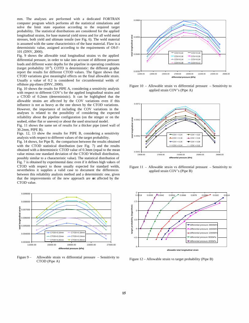
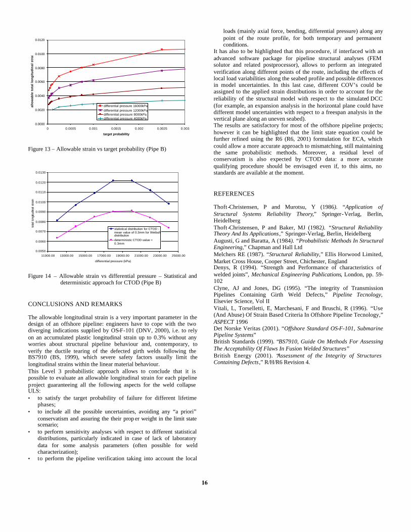
mm. The analyses are performed with a dedicated FORTRAN computer program which performs all the statistical simulations and solve the limit state equation according to the required target probability. The statistical distributions are considered for the applied longitudinal strains, for base material yield stress and for all weld metal stresses, both yield and ultimate tensile (see Fig. 6). The weld material is assumed with the same characteristics of the base material. Flaw is a deterministic value, assigned according to the requirements of OS-F-101 (DNV, 2000). Fig. 9 shows the allowable total longitudinal strains vs the applied differential pressure, in order to take into account of different pressure loads and different water depths for the pipeline in operating conditions (target probability 10-4). COTD is deterministic: the different graphs report the results for different CTOD values. The figure shows that CTOD variations give meaningful effects on the final allowable strain. Usually a value of 0.2 is considered for circumferential welds of offshore pip elines (DNV, 2000). Fig. 10 shows the results for PIPE A, considering a sensitivity analysis with respect to different COV’s for the applied longitudinal strains and a CTOD of 0.2mm (deterministic). It can be highlighted that the allowable strains are affected by the COV variations even if this influence is not as heavy as the one shown by the CTOD variations. However, the importance of including the COV variations in the analyses is related to the possibility of considering the expected reliability about the pipeline configuration (on the stinger or on the seabed, either flat or uneven) or about the used structural model. Fig. 11 shows the same set of results for a thicker pipe (steel wall of 30.2mm, PIPE B). Figs. 12, 13 show the results for PIPE B, considering a sensitivity analysis with respect to different values of the target probability. Fig. 14 shows, for Pipe B, the comparison between the results obtained with the CTOD statistical distribution (see Fig. 7) and the results obtained with a deterministic CTOD value of 0.3mm (equal to the mean value minus one standard deviation of the CTOD Weibull distribution, possibly similar to a characteristic value). The statistical distribution of Fig. 7 is obtained by experimental data: even if it defines high values of CTOD with respect to those usually expected for standard welds, nevertheless it supplies a valid case to document the differences between this reliability analysis method and a deterministic one, given that the improvements of the new approach are not affected by the CTOD value.

0.003000

0.004000

0.005000

0.006000

0.007000

0.008000

0.009000

11000.00 15000.00 19000.00 23000.00 27000.00

differential pressure (kPa)

tota

l lon

gitu

dina

l str

ain

CTOD=0.16mm CTOD=0.18mm



Figure 9 – Allowable strain vs differential pressure – Sensitivity to CTOD (Pipe A)

0.0039

0.0049

0.0059

0.0069

11000.00 13000.00 15000.00 17000.00 19000.00 21000.00 23000.00 25000.00


tota

l lo

ng

itu

din

al s

trai

n

COV=0.22 COV=0.18

COV=0.16 COV=0.26

COV=0.14 COV=0.24

COV=0.28 COV=0.12

Figure 10 – Allowable strain vs differential pressure – Sensitivity to applied strain COV’s (Pipe A)

0.0042

0.0052

0.0062

0.0072

13000.00 17000.00 21000.00 25000.00 29000.00


tota

l lo

ng

itu

din

al s

trai

nCOV = 0.24 COV = 0.22

COV = 0.18 COV = 0.16

COV = 0.26 COV = 0.28

COV = 0.14 COV = 0.12

Figure 11 – Allowable strain vs differential pressure – Sensitivity to applied strain COV’s (Pipe B)

-5

-4.5

-4

-3.5

-3

-2.5

-20.0018 0.0030 0.0042 0.0054 0.0066 0.0078 0.0090 0.0102 0.0114

allowable total longitudinal strain

targ

et p

rob

abil

ity

(lo

gar

ith

mic

)

differential pressure 28000kPa





Figure 12 – Allowable strain vs target probability (Pipe B)

15

0.0000

0.0020

0.0040

0.0060

0.0080

0.0100

0.0120

0 0.0005 0.001 0.0015 0.002 0.0025 0.003

target probability

allo

wab

le t

ota

l lo

ng

itu

din

al s

trai

n

differential pressure 16000kPadifferential pressure 12000kPadifferential pressure 8000kPadifferential pressure 4000kPa

Figure 13 – Allowable strain vs target probability (Pipe B)

0.0050

0.0060

0.0070

0.0080

0.0090

0.0100

0.0110

0.0120

0.0130

11000.00 13000.00 15000.00 17000.00 19000.00 21000.00 23000.00 25000.00


tota

l lon

gitu

dina

l stra

in

statistical distribution for CTOD -mean value of 0.3mm for Weibulldistributiondeterministic CTOD value =0.3mm

Figure 14 – Allowable strain vs differential pressure – Statistical and deterministic approach for CTOD (Pipe B)

CONCLUSIONS AND REMARKS The allowable longitudinal strain is a very important parameter in the design of an offshore pipeline: engineers have to cope with the two diverging indications supplied by OS-F-101 (DNV, 2000), i.e. to rely on an accumulated plastic longitudinal strain up to 0.3% without any worries about structural pipeline behaviour and, contemporary, to verify the ductile tearing of the defected girth welds following the BS7910 (BS, 1999), which severe safety factors usually limit the longitudinal strains within the linear material behaviour. This Level 3 probabilistic approach allows to conclude that it is possible to evaluate an allowable longitudinal strain for each pipeline project guaranteeing all the following aspects for the weld collapse ULS: • to satisfy the target probability of failure for different lifetime

phases; • to include all the possible uncertainties, avoiding any “a priori”

conservatism and assuring the their prop er weight in the limit state scenario;

• to perform sensitivity analyses with respect to different statistical distributions, particularly indicated in case of lack of laboratory data for some analysis parameters (often possible for weld characterization);

• to perform the pipeline verification taking into account the local

loads (mainly axial force, bending, differential pressure) along any point of the route profile, for both temporary and permanent conditions.

It has also to be highlighted that this procedure, if interfaced with an advanced software package for pipeline structural analyses (FEM solutor and related postprocessor), allows to perform an integrated verification along different points of the route, including the effects of local load variabilities along the seabed profile and possible differences in model uncertainties. In this last case, different COV’s could be assigned to the applied strain distributions in order to account for the reliability of the structural model with respect to the simulated DCC (for example, an expansion analysis in the horizontal plane could have different model uncertainties with respect to a freespan analysis in the vertical plane along an uneven seabed). The results are satisfactory for most of the offshore pipeline projects; however it can be highlighted that the limit state equation could be further refined using the R6 (R6, 2001) formulation for ECA, which could allow a more accurate approach to mismatching, still maintaining the same probabilistic methods. Moreover, a residual level of conservatism is also expected by CTOD data: a more accurate qualifying procedure should be envisaged even if, to this aims, no standards are available at the moment. REFERENCES Thoft -Christensen, P and Murotsu, Y (1986). “Application of Structural Systems Reliability Theory,” Springer-Verlag, Berlin, Heidelberg Thoft -Christensen, P and Baker, MJ (1982). “Structural Reliability Theory And Its Applications ,” Springer-Verlag, Berlin, Heidelberg Augusti, G and Baratta, A (1984). “Probabilistic Methods In Structural Engineering,” Chapman and Hall Ltd Melchers RE (1987). “Structural Reliability,” Ellis Horwood Limited, Market Cross House, Cooper Street, Chichester, England Denys, R (1994). “Strength and Performance of characteristics of welded joints”, Mechanical Engineering Publications, London, pp. 59-102 Clyne, AJ and Jones, DG (1995). “The integrity of Transmission Pipelines Containing Girth Weld Defects,” Pipeline Tecnology, Elsevier Science, Vol II Vitali, L, Torselletti, E, Marchesani, F and Bruschi, R (1996). “Use (And Abuse) Of Strain Based Criteria In Offshore Pipeline Tecnology,” ASPECT 1996 Det Norske Veritas (2001). “Offshore Standard OS-F-101, Submarine Pipeline Systems” British Standards (1999). “BS7910, Guide On Methods For Assessing The Acceptability Of Flaws In Fusion Welded Structures” British Energy (2001). “Assessment of the Integrity of Structures Containing Defects ,” R/H/R6 Revision 4.

16

structural reliability approach to strain based design of offshore pipelines

Documents