reliability and availability modeling in practice
TRANSCRIPT

Reliability and Availability Modeling in Practice
IFIP 7.3 Performance Conference -- TutorialNov. 2, 2020
1

IFIP 7.3 Performance Conference 2020
Students may get a certificate for participation in this Tutorial
You need to fill in a google form:
https://docs.google.com/forms/d/e/1FAIpQLSe9Fgh5rdxcP9RLPMktHUHrGXZlMGKuxKC_7JICedzQWjrVyw/viewform
2

Tutorial Objective
To provide an overview and state of the art of analytic methods for reliability and availability assessment
To provide real-life examples that show the use of analytic methods in practice
To provide current challenges faced in such modeling projects
Ref: Trivedi & Bobbio, Reliability and Availability: Modeling, Analysis, Applications, Cambridge University Press, 2017
3

Tutorial Outline
Introduction Reliability and Availability Models Model Types in Use Illustrated through several real examples
Conclusions References
4
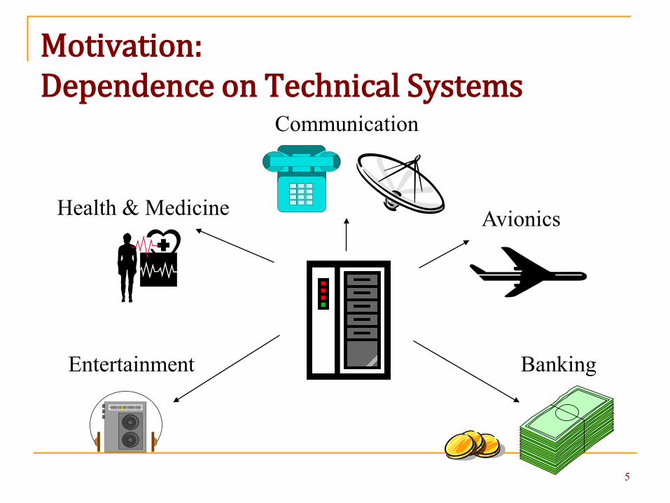
Health & Medicine
Communication
Avionics
Entertainment Banking
Motivation: Dependence on Technical Systems
5

Example Failures from High Tech companies
Mar. 2015 , Gmail was down for 4 hours and 40 min.
Mar. 2015, Down for 3 hours affecting Europe and US
Sept. 2015, AWS DynamoDB down for 4 hours impacting among others Netflix, AirBnB, Tinder
Dec. 2015, Microsoft Office 365 and Azure down for 2 hours
Mar. 2015, Apple ITunes, App Stores long 0utage: 12 hours
6

More examples of real failures
Feb. 2017 Amazon S3 service outage (almost 6 hours)
Jul. 2017 - Google Cloud Storage service outage (3 hours and 14 min.) - API low-level software defect
Jul. 2017 - Microsoft Azure service outage (4 hours) –Load Balancer Software bug
7

Very Recent Examples
In Commercial aircrafts (Boeing 737 Max software problem) Ethiopian Airlines Flight, March 2019,
149 people died Lion Air Flight crash, Oct. 2018,
189 people died

Need Methods
That reduce the occurrence of system failures and reduce downtime due to these failures (contributed by hardware, software and humans)
For System Reliability/Availability assessment and bottleneck detection during: Design phase Certification phase Operational phase
9

Introduction
10
Basic Definitions

Need for a new term
Reliability is often used in a generic sense as an umbrella term.
Reliability is also used as a precisely defined mathematical function.
To remove the confusion, IFIP WG 10.4 proposed Dependability as an umbrella term and Reliability is to be used as a well-defined mathematical function.
11

Dependability– An umbrella term
Trustworthiness of a system such that reliance can justifiably be placed on the service it delivers
Dependability
AttributesAvailabilityReliabilitySafetyMaintainability
Fault PreventionFault RemovalFault ToleranceFault Forecasting
Means
ThreatsFaultsErrorsFailures
12

Difference between reliability and availability
13
reliability refers to failure-free operation during an entire interval,
availability refers to failure-free operation at a given instant of time.
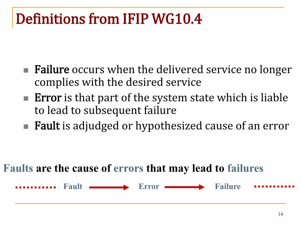
Definitions from IFIP WG10.4
Failure occurs when the delivered service no longer complies with the desired service
Error is that part of the system state which is liable to lead to subsequent failure
Fault is adjudged or hypothesized cause of an error
Faults are the cause of errors that may lead to failuresFault Error Failure
14

A Classification of Faults
Hardware vs. Software vs. Human Hardware: Permanent, Intermittent, Transient Network: Node vs. Link Software: Bohrbugs, Mandelbugs, Heisenbugs, Aging-
related bugs

Failure Classification
Omission failures (Send/receive failures) Crash failures Infinite loop
Response or Value failures Timing failures
Early Late (aka performance failure or dynamic failures)
Safe vs. Unsafe failure Breach of confidentiality or breach of integrity or loss of use

Basic Definitions
One shot Reliability R:
When is this applicable?
Reliability R(t) :X : Time to failure of a system (TTF), or lifetime random variableF(t): distribution function of system lifetime
Reliability is the complementary distribution function of TTF
( ) ( ) ( )tFtXPtR −=>= 1
17

Basic Definitions
Mean Time To system Failure:
where f(t): density function of system lifetime
[ ] ( ) ( )∫∫∞∞
===00
dttRdtttfXEMTTF
Make a clear distinction between TTF, R(t) and MTTF
18

Basic Definitions
Availability
Operating and providingrequired functions
Failed andbeing restored
1
0
Operating and providingrequired functions
System Failure and Restoration ProcessI(t) is the indicator function
I(t)
19

Basic Definitions
Instantaneous Availability A(t):
From the figure in the last slide, the availability at time tbecomes:
This is sometimes called point-wise availability,instantaneous availability, or transient availability. A(t)can be asked for at any point t in time
A(t) = P (system working at t)
A(t)=P(I(t)=1)
20

Basic Definitions
Interval reliability measure introduced by Barlow and Hunter in 1961, combines availability A(t) and reliability R(τ) : Available when needed (at time t) & as long as needed (for τ time units)
Interval reliability further developed in: Trivedi & Bobbio, Reliability and Availability: Modeling, Analysis,
Applications, Cambridge University Press, 2017
Wang & Trivedi, Modeling User-Perceived Service Reliability based User-Behavior Graphs, IJRQS, 2011
Trivedi, Wang & Hunt, Computing the number of calls dropped due to failures, ISSRE2010
Mondal, Yin, Muppala, Alonso, Trivedi, Defects per Million Computation in Service-Oriented Environments, IEEE Trans. on Services Comp., 2015
21
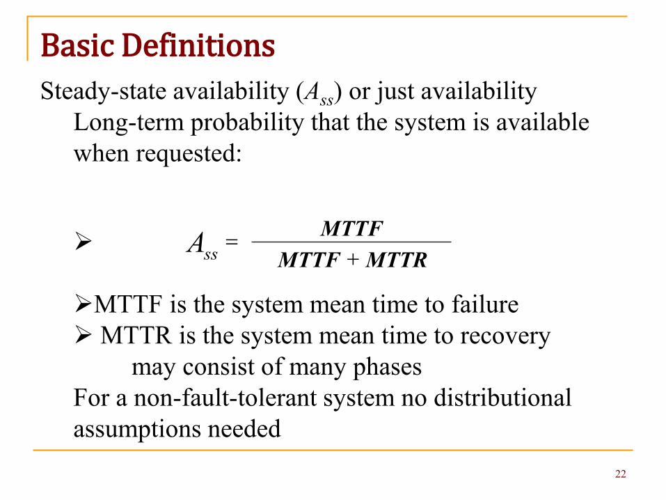
Basic DefinitionsSteady-state availability (Ass) or just availability
Long-term probability that the system is available when requested:
MTTF is the system mean time to failureMTTR is the system mean time to recovery
may consist of many phasesFor a non-fault-tolerant system no distributional assumptions needed
MTTRMTTFMTTF
+=
ssA
22

Basic Definitions
Steady-state availability (Ass) or just availability Long-term probability that the system is available when requested (also applies to a fault-tolerant system):
MTTF is the “equivalent” system mean time to failure, a complex combination of component MTTFsMTTR is the “equivalent” system mean time to recovery
MTTRMTTFMTTF
+=ssA
23

Basic Definitions
Downtime in minutes per year In industry, steady-state (un)availability is usually
presented in terms of annual (steady-state) downtime.
Downtime = 8760×60 ×(1- Ass) minutes.
It is also common to define the availability in terms of number of nines
5 NINES (Ass = 0.99999) 5.26 minutes annual downtime4 NINES (Ass = 0.9999) 52.56 minutes annual downtime
24

Number of Nines– Reality Check
49% of Fortune 500 companies experience at least 1.6 hours of downtime per week
Approx. 80 hours/year=4800 minutes/year
Ass=(8760-80)/8760=0.9908
That is, between 2 NINES and 3 NINES!
This study combines planned and unplanned downtime
25

Failures & Downtime Lead to
A Loss of Reputation A Loss of Revenue Possible Loss of Life
26

That reduce system failures and reduce downtime due to these failures (contributed by hardware, software and humans)
System Reliability/Availability assessment and bottleneck detection methods can be used: To compare alternative designs/architectures Find bottlenecks, answer what if questions, design optimization
and conduct trade-off studies At certification time At design verification/testing time Configuration selection phase Operational phase for system tuning/on-line control
Need Methods
27

Methods to Improve Dependability
Fault Avoidance Employ high reliability components
Fault Removal Careful Testing to remove faults
Fault Tolerance Utilize Redundancy
Fault Forecasting Predict failures and use for preventive maintenance
28

Methods Overview (Redundancy)
Redundancy
Coding
Time
Use of Multiple Redundant Components, that is,
more than required for the performance needs29

Methods Overview (Redundancy)
Time
Retry
Restart
Checkpoint/restart
Multiple components
ParallelIdentical
Non-identical
k of nIdentical
Non-identical
Standby
Cold
Warm
Hot
CodingHamming
CRC
30
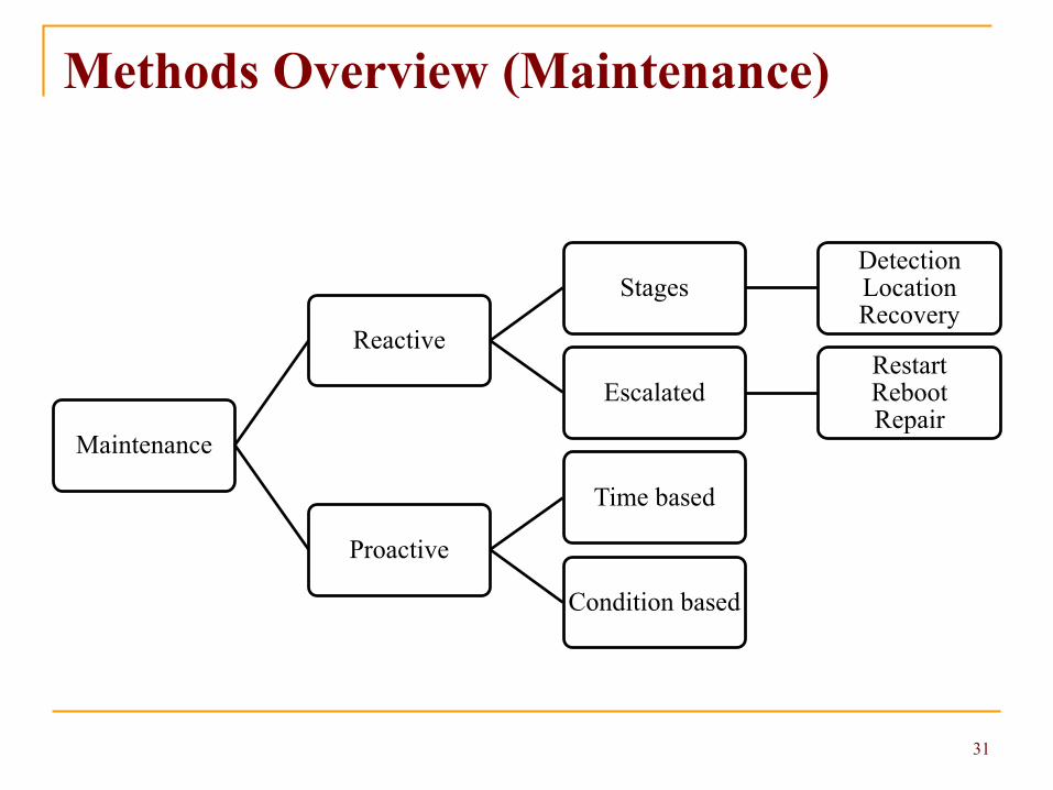
Methods Overview (Maintenance)
Maintenance
Reactive
StagesDetectionLocationRecovery
EscalatedRestartRebootRepair
Proactive
Time based
Condition based
31

That reduce system failures and reduce downtime due to these failures (contributed by hardware, software and humans)
System Reliability/Availability assessment and bottleneck detection methods can be used: To compare alternative designs/architectures Find bottlenecks, answer what if questions, design optimization
and conduct trade-off studies At certification time At design verification/testing time Configuration selection phase Operational phase for system tuning/on-line control
Need Methods
32

Quantitative Assessment approaches
Black-box or Data-driven(measurement data + statistical inference):
The system is treated as a monolithic whole, without explicitly taking its internal structure into account
Very expensive especially for ultra-reliable systems ALT can help reduce the cost
Generally applicable to small systems that are not very highly reliable
Not feasible for system under design/development
33

Quantitative Assessment approaches White-box (or Model-driven): When no data is available for the system as a whole Probability Model (e.g., RBD, Ftree, Markov chain)
constructed based on the known internal structure of system – its components, their characteristics and interactions between components
Derive the behavior of ensembles (combinations of components to form a system or combinations of multiple systems to form a system of systems) from first principles
Used to analyze a system with many interacting and interdependent components
Need input parameters for components and subsystems34
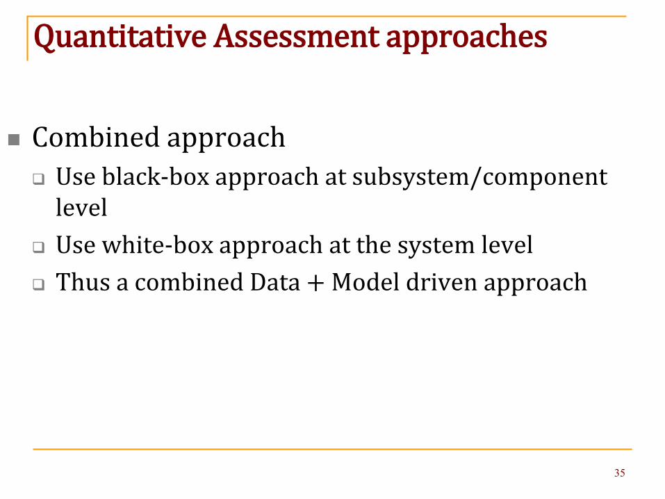
Quantitative Assessment approaches
Combined approach Use black-box approach at subsystem/component
level Use white-box approach at the system level Thus a combined Data + Model driven approach
35

Two Types of Uncertainty
Aleatory (irreducible) Randomness of event occurrences in the real system
captured by various distributions in the Probability Model (e.g., RBD, Fault tree, Markov chain)
Epistemic (reducible) Introduced due to finite sample size in estimating
parameters to be input to the Probability Model Propagating epistemic uncertainty through a
Probability Model is a topic that will not be covered in this tutorial – can be a subject of another tutorial!
36

Outline
Introduction and Motivation Reliability and Availability Models Conclusions References
37

Overview of Assessment Methods
Numerical solution via a tool
Closed-formsolution
Model-driven
Discrete-event simulation
Hybrid
Analytic methodsNumerical solutionof analytic modelsnot as well utilized;unnecessarily excessiveuse of simulation
Quantitative Assessment
Data-driven Error/Failure/Recovery data analytics
38

Analytic Methods Taxonomy
Hierarchical composition
Fixed point iterative methods
Analytic methods
Non-state-space methods
State-space methods
Model-driven
Discrete-event simulation
Hybrid
Analytic Methods
Quantitative Assessment
Data-driven
39

Non-State-Space Methods : taxonomy
Non-state space methods
SP reliability block diagrams (RBD)
Fault trees
Fault trees with repeated events
Non-SP reliability block diagrams (relgraph)
Extensions such as multi-state components/systems, phased-mission systems etc.
40

Cisco & Juniper Routers
RBD of Cisco 12000 GSR
RBD of Juniper M20 K. Trivedi, “Availability Analysis of Cisco GSR 12000 and Juniper M20/M40” Cisco Internal report, 2000.Red colored block means a sub-model.
41

Modeling High Availability Systems: Sun Microsystems
Top level RBD consists of all the subsystems joined by series, parallel and k/n blocks.Red color means a sub-model.
Trivedi et al., Modeling High Availability Systems, PRDC’06 Conference, Dec. 2006, Riverside, CA
Sun Microsystems
42

Series-Parallel RBDs
System reliability (availability) formulas : Assuming statistical Independence of failures (and repairs) Reliabilities (availabilities) multiply for blocks in series
Un-reliabilities (un-availabilities) multiply for blocks in parallel
Blocks in k-out-of-n have a simple formula Identical case Rk|n= ∑𝑗𝑗=𝑘𝑘𝑛𝑛 𝑛𝑛
𝑗𝑗 𝑅𝑅𝑗𝑗(1 − 𝑅𝑅𝑛𝑛−𝑗𝑗
Non-identical case
>=
=
⋅+⋅−= −−−
ijRR
RRRRR
ij
n
nknnknnk
when ,01
)1(
|
|0
1|11||
43
∏=
=n
iis RR
1

Fault Trees
Fault Tree is a pessimist’s model as opposed to RBD that can be considered optimists’ models
Components are represented as leaves or terminal nodes
Internal nodes are logic gates and Root node indicates system failure
Components or subsystems in series are connected with OR gates
Components or subsystems in parallel are connected with AND gates
Failure of a component or subsystem causes the corresponding input to the gate to become TRUE
Whenever the output of the topmost gate (root node) is TRUE, the system is considered failed
44
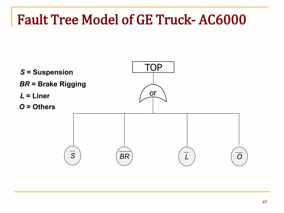
Fault Tree Model of GE Truck- AC6000
TOPS = SuspensionBR = Brake RiggingL = LinerO = Others
S OLBR
45

Fault Tree Model of GE Equipment Ventilation System
Fault Tree with Repeated events; inverted triangle indicates such events
46

47

Software Package SHARPE
SHARPE: Symbolic-Hierarchical Automated Reliability and Performance Evaluator
Stochastic Modeling tool installed at over 1000 Sites; companies and universities
Ported to most architectures and operating systems Used for Education, Research, Engineering Practice Users: Boeing, 3Com, EMC, AT & T, Alcatel-Lucent, IBM,
NEC, Motorola, Siemens, GE, HP, Raytheon, Honda,… http://sharpe.pratt.duke.edu/ It is the core of Boeing’s internal tool called IRAP
A Fool with a Tool is still a fool
48

Fault trees
Major characteristics: Fault trees without repeated events can be solved in polynomial
time Fault trees with repeated events -Theoretical complexity:
exponential in number of components
Use Factoring (conditioning) [In SHARPE use factor on and bdd off]
Find all minimal cut-sets & then use Sum of Disjoint products (SDP) to compute reliability [In SHARPE use factor off and bdd off]
Use BDD (Binary Decision Diagram) approach [In SHARPE use bdd on]
In practice, can solve fault trees with thousands of components
49

Solution time for Very Large Fault trees
50
Such large models can be solved because of independence assumption – non-states-space models
Fault Trees (Continued)
Extensions to Fault-trees include a variety of different gate
types: NOT, EXOR, Priority AND, cold spare gate,
functional dependency gate, sequence enforcing gate, etc.
Some of these are “static” while others are “dynamic”
gates
51

Reliability Graph (relgraph)
Consists of a set of nodes and edges
Edges represent components that can fail
Source and target (sink) nodes
System fails when no path from source to sink
A non-series-parallel RBD
S-t connectedness or network reliability problem
52

Relgraphs
Solution methods for Relgraph Find all minpaths followed by SDP (Sum of Disjoint
Products) BDD (Binary Decision Diagrams)-based method Factoring or conditioning Monte Carlo method
The first two methods have been implemented in our SHARPE software package
53

Avionics
Reliability analysis of each major subsystem of a commercial airplane needs to be carried out and presented to Federal Aviation Administration (FAA) for certification
Real world example from Boeing Commercial Airplane Company
55
Reliability Analysis of Boeing 787
Most of the subsystems are improved or modified versions of subsystems used in earlier planes Models are also modified version of the earlier
models Occasionally there is an entirely new subsystem
Model needs to be done from scratch Current Return Network in Boeing 787 is one such
example Several of my former students are in the Boeing
Reliability Engineering group
56

Reliability Analysis of Boeing 787
Current Return Network Subsystem Modeled as a Reliability Graph Consists of a set of nodes and edges Edges represent components that can fail Source and target nodes System fails when no path from source to
target Compute probability of a path from source to
target
57

Reliability Analysis of Boeing 787
A2
A4
A5
A1
A11
A13
A14
A7
A8
A9
A6
A10
A3B3
B4
B6
B1
B13
B14
B15
B8
B9
B10
B7
B11
B2
B12
A12
B5
B16
C1
C3
C4
C5
C2
C6
D3
D5
D7
D1
D16
D17
D19
D9
D12
D13
D8
D14
D2
D15
D4
D18
D6
D10
D20
D11E6
E7
E8
E5
E1
E2
E3
E4
E10
E11
E12
E9
E14
E13
target
F1
F8
F3
F2F4
F5
F6
F9
F7
F10
source
Current Return Network Modeled as a Reliability Graph
58

Reliability Analysis of Boeing 787 (cont’d)
Solution methods implemented in our SHARPE software package for relgraph Find all minpaths followed by SDP (Sum of Disjoint
Products) BDD (Binary Decision Diagrams)-based method
Boeing tried to use SHARPE for this problem but …
59

Reliability Analysis of Boeing 787 (cont’d)
A2
A4
A5
A1
A11
A13
A14
A7
A8
A9
A6
A10
A3B3
B4
B6
B1
B13
B14
B15
B8
B9
B10
B7
B11
B2
B12
A12
B5
B16
C1
C3
C4
C5
C2
C6
D3
D5
D7
D1
D16
D17
D19
D9
D12
D13
D8
D14
D2
D15
D4
D18
D6
D10
D20
D11E6
E7
E8
E5
E1
E2
E3
E4
E10
E11
E12
E9
E14
E13
target
F1
F8
F3
F2F4
F5
F6
F9
F7
F10
source
Too many minpaths
Idea: Compute bounds instead of exact reliability Lower bound by taking a subset of minpaths Upper bound by taking a subset of mincuts
60

Reliability Analysis of Boeing 787 (cont’d)
Our Approach : Developed a new efficient algorithm for (un)reliability bounds computation and incorporated in SHARPE
• 2011 patent for the algorithm jointly with Boeing/Duke • “Fast computation of bounds for two-terminal network reliability”, EJOR 2014• Satisfying FAA that SHARPE development used DO-178 B software standard
was the hardest part• As per A.V. Ramesh (Boeing), this algorithm (and SHARPE) are always used
for modeling CRN subsystem in other Boeing commercial aircraft
61

RBD->Relgraph->ftree
Series-parallel RBD and Fault trees without repeated event are equivalent
Relgraph is more powerful than RBD since non-series-parallel behavior can be accommodated
Fault trees with repeated event are more powerful than relgraphs
Most scalable method is the bounding algorithm for relgraphs; this needs to be extended to fault trees
62

Power-hierarchy of modeling formalisms
State space
Non-State space
63

Non-state-space Methods (cont’d) Non-state-space methods are easy to use and have relatively fast
algorithms for system reliability, system availability, system MTTF & tofind bottlenecks assuming stochastic independence between systemcomponents Series-parallel composition algorithm Factoring (conditioning) algorithms All minpaths followed by Sum of Disjoint Products (SDP) algorithm Binary Decision Diagrams (BDD) based algorithms Bounding algorithm for relgraphs
All of the above implemented in SHARPE
Failure/Repair Dependencies are often present; RBDs, relgraphs,FTREEs cannot easily handle these (e.g., shared repair, warm/coldspares, imperfect coverage, non-zero switching time, travel time ofrepair person, reliability with repair).
64

Statistical Dependence
The independence assumption is often unrealistic
65
Dependencies in the failure process are load dependencies, functional dependencies, cascading failures common cause failures Coincident (or near-coincident) faults
Dependencies in the repair process deferred maintenance shared repair facilities.
R. Fricks and K. Trivedi, “Modeling failure dependencies in reliability analysis using stochastic Petri nets,” in Proc. European Simulation Multi-Conference (ESM ’97), 1997.

State-space methods : Markov chains
To model complex interactions between components, need to use paradigms like Markov chains or more generally state space models.
Many examples of dependencies among system components have been observed in practice and captured by continuous-time Markov chains (CTMCs).
Extension to Markov reward models makes computation of measures of interest relatively easy.
66
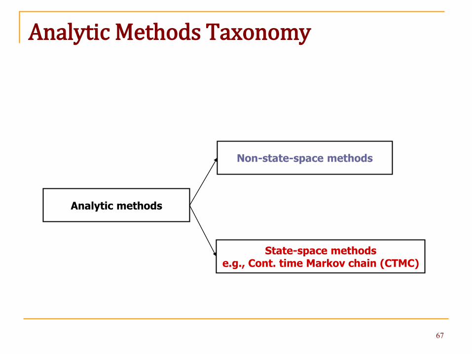
Analytic Methods Taxonomy
Analytic methods
Non-state-space methods
State-space methodse.g., Cont. time Markov chain (CTMC)
67

Markov model of SIP on IBM WebSphere
A CTMC availability model of the Linux OS
UP DN DWλOS
µOS
RPαsp
bOSβOS
(1-bOS)βOSDT
δOS
Detection delay, imperfect coverage, two-levels of recovery modeled
How can you turn this into a reliability model?
68

A CTMC Reliability model of the Linux OS
69
A reliability model will have one or more absorbing statesAn availability model will have no absorbing states
An absorbing state

SHARPE Input file for the Linux Modelecho Linux OS Availability Modelmarkov LinuxOS1 2 los2 3 dos3 1 bos*beta3 4 (1-bos)*beta4 5 asp5 1 mosend
* Parameter values in per hrbind los 1/4000dos 1beta 6bos 0.9asp 1/2mos 1end
echo Steady-state availability equal to probability of state UP
expr prob (LinuxOS,1)
end
70

SHARPE Output file for the Linux Model
Linux OS Availability Model
Steady-state availability equal to probability of state UP
prob (LinuxOS,1): 9.99633468e-001
71

SHARPE Input file for the Linux Reliability Model (state 4 absorbing)echo Linux OS Reliability Modelmarkov LinuxOS1 2 los2 3 dos3 1 bos*beta3 4 (1-bos)*betaend* initial state probabilities1 1.02 0.03 0.04 0.0end
* Parameter valuesbind los 1/4000dos 1beta 6bos 0.9asp 1/2mos 1end
echo Reliability at times 0 thru 10000 in steps of 2000 equal to probability of state 1func rel(t) tvalue(t;LinuxOS,1)loop t,0, 10000, 2000expr rel(t)endend
72

SHARPE Input file for the Linux Reliability Model (state 4 absorbing)
Linux OS Reliability ModelReliability vs time equal to probability of state 1
at time tSystem reliability at times 0 thru 10000 in steps of 2000
t=0.000000rel(t): 1.00000000e+000
t=2000.000000rel(t): 9.50987909e-001
t=4000.000000rel(t): 9.04617746e-001
t=6000.000000rel(t): 8.60508971e-001
t=8000.000000rel(t): 8.18551046e-001
t=10000.000000rel(t): 7.78639141e-001
73

Markov (CTMC) Availability model of App Server
Application server and proxy server (with escalated levels of recovery)
Delay and imperfect coverage in each step of detection/recovery modeled
UA UR UB(1-r)ρm
rρmqρa
(1-q)ρa
bβm
RE(1-b)βm
µ
UOUPγ eδ2
1D
eδ2dδ1
(1-e)δ2
UN
δm
1N
(1-d)δ1
(1-e)δ2
2N (1-d)δ1
(1-e)δ2
eδ2 dδ1
Failure detection By WLM By Node Agent Manual detection
Recovery Node Agent
Auto process restart
Manual recovery Process restart Node reboot Repair
74

CTMC with Infinitesimal Generator matrix Q Efficient/Scalable algorithms are known & are
implemented in software packages SHAREPE, SPNP for: Steady-state behavior:
Transient behavior:
Cumulative Transient behavior:
Also derivatives of the probabilities with respect to parameters – parametric sensitivity functions are computed 75
1,0 == ∑i
iQ ππ
)0(,)()( πππ givenQtdt
td=
dL(t)/dt = L(t) Q + π (0) L(t): integrals of state probability vector

State-Space methods taxonomy
Can relax the assumption of exponential distributions
(discrete) State space models
Markovian models
non-Markovian models
discrete-time Markov chains (DTMC)
continuous-time Markov chains (CTMC)
Markov reward models (MRM)
Semi-Markov process (SMP)
Markov regenerative process
Non-Homogeneous Markov
Phase-Type Expansion
76

Should I Use Markov (CTMC) Models?
+ Model Fault-Tolerance and Recovery/Repair
+ Model Dependencies
+ Model Contention for Resources and concurrency (performance)
+ Generalize to Markov Reward Models for Degradable systems
+ Can relax exponential assumption – SMP, MRGP, NHCTMC, PH
+ Performance, Availability, Performability, Survivability, Resilience Modeling Possible
- Large State Space
77

Markov Models Modeling inter-dependence among components
Simple model types such as RBD, Ftree, etc. do not suffice –need to use Markov and other state space model types
State space explosion problem
78

Problems with Markov (or State Space) Models and their solutions State space explosion or the model
largeness problem or scalability problem Stochastic Petri nets and related formalisms
(stochastic process algebras) for ease of specification and automated generation/solution of underlying Markov model ---
This is called Largeness Tolerance
79

Scalable Model for IaaS Cloud Availability and Downtime
Ref: Ghosh, Longo, Frattini, Russo, Trivedi,“Scalable Analytics for IaaS Cloud Availability,”
IEEE Trans. Cloud Comput., 2014
80

Three Pools of Physical Machines (PMs)To reduce power usage costs, physical machines are divided into three pools [IBM Research Cloud]
Hot pool (high performance & high power usage) Warm pool (medium performance & power usage)Cold pool (lowest performance & power usage)
Similar grouping of PMs is recommended by Intel*
*Source: http://www.intel.com/content/dam/www/public/us/en/documents/guides/lenovo-think-server-smart-grid-technology-cloud-builders-guide.pdf
81

System Operation Details
Failure/Repair (Availability): PMs may fail and get repaired.A minimum number of operational hot PMs are
required for the system to function. PMs in other pools may be temporarily assigned to the
hot pool to maintain system operation (migration).Upon repair, PMs migrate back to their original poolMigration creates dependence among pools
82

Analytic model Markov model (CTMC) is too large to construct by hand. We use a high-level formalism of stochastic Petri net (the
flavor known as stochastic reward net (SRN)). SRN models can be automatically converted into underlying
Markov (reward) model and solved for the measures of interest such as DT (downtime), steady-state (instantaneous, interval) availability, reliability, derivatives of these measures --- all numerically by forming and solving underlying equations
Analytic-numeric solution as opposed to discrete-event simulation
Ref: Ciardo, Blakemore, Chimento, Muppala, Trivedi, “Automated generation and analysis of Markov reward models using stochastic reward nets,” Linear Algebra, Markov Chains, and Queueing Models, Springer, 1993
83

Monolithic Stochastic Reward Net Model
84
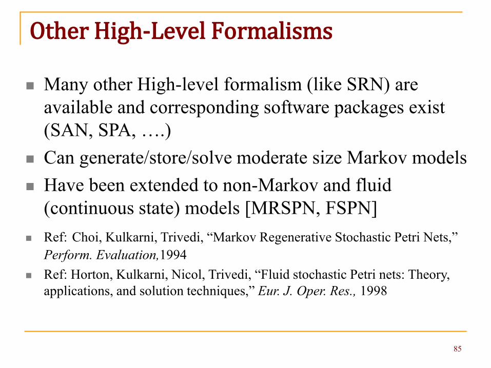
Other High-Level Formalisms
Many other High-level formalism (like SRN) are available and corresponding software packages exist (SAN, SPA, ….)
Can generate/store/solve moderate size Markov models Have been extended to non-Markov and fluid
(continuous state) models [MRSPN, FSPN] Ref: Choi, Kulkarni, Trivedi, “Markov Regenerative Stochastic Petri Nets,”
Perform. Evaluation,1994 Ref: Horton, Kulkarni, Nicol, Trivedi, “Fluid stochastic Petri nets: Theory,
applications, and solution techniques,” Eur. J. Oper. Res., 1998
85

Monolithic ModelMonolithic SRN model is automatically translated into CTMC or Markov Reward ModelHowever the model not scalable as state-space size of this model is extremely large#PMs per pool #states #non-zero matrix entries
3 10, 272 59, 560
4 67,075 453, 970
5 334,948 2, 526, 920
6 1,371,436 11, 220, 964
7 4,816,252 41, 980, 324
8 Memory overflow Memory overflow
10 - -
86

Problems with Markov (or State Space) Models and their solutions
State space explosion or the largeness problem Stochastic Petri nets and related formalisms for easy
specification and automated generation/solution of underlying Markov model --- Largeness Tolerance
Use hierarchical (Multilevel) model composition Largeness Avoidance e.g. Upper level : FT or RBD, lower level: Markov chains Many practical examples of the use of hierarchical
models exist Can also use state truncation
87

Analytic Modeling Taxonomy
Hierarchical compositionTo avoid largeness
Analytic models
Non-state-space methodsEfficiency, simplicity
State-space methodsDependency capture
88

State Space Explosion Number of components in systems can be hundreds,
nay thousands! Number of states in a Markov model will be a
gazillion! State space explosion can be avoided by decomposing
system into subsystems, modeling each subsystem separately and then composing sub-model results together – SHARPE facilitates this
Use state-space methods for those subsystems that require them, and use simple non-state-space methods (RBD, Ftree) for the more “well-behaved” parts of the system
89

Largeness Avoidance Main reason for hierarchical (or multilevel) models: avoid
generating/solving large monolithic models; that is for tractability
In SHARPE we can mix and match different paradigms and to arbitrary levels
Can choose the “right” paradigm for each subsystem Note that some tools/approaches use hierarchy merely for
specification and a monolithic model is constructed by the tool We are advocating hierarchy not only for specification but also
for solution Hierarchy does not always mean an approximation Most practical problems I have solved have 2 or more levels
with the top level being RBD/ftree and Markov models at the lowest level
90

Availability Analysis: SUN Microsystems
Carrier-Grade High Availability Software Platform Model taking into account hardware component
failures, software component failures and varioustypes of recovery
Hierarchical model composition – Markov chainsat the lower-level, RBD at the top level
Ref: Trivedi, Vasireddy, Trindade, Nathan, Castro, “Modeling HighAvailability Systems,” Proc. PRDC 2006.
91

Sun Microsystems – overall model hierarchy
…
92
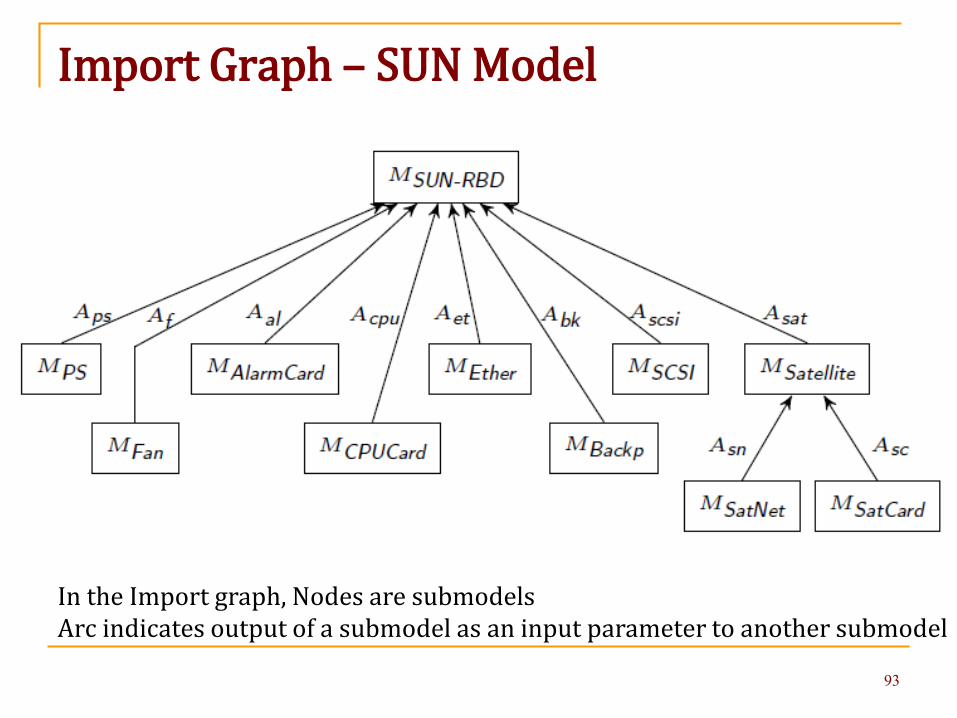
Import Graph – SUN Model
93
In the Import graph, Nodes are submodelsArc indicates output of a submodel as an input parameter to another submodel

High-Availability SIP System Real problem from IBM
SIP: Session Initiation Protocol
Hardware platform: IBM Blade Center
Software platform: IBM WebSphere
A Telco (potential) customer asked IBM for models to quantify this product
IBM asked me to lead the modeling project
To quantify system (steady-state) availability Ref: Trivedi, Wang, Hunt, Rindos, Smith, Vashaw, “Availability Modeling of SIP Protocol on IBM WebSphere,” PRDC 2008
To quantify a user-oriented metric called DPM Ref: Trivedi, Wang & Hunt. “Computing the number of calls dropped due to failures,” ISSRE2010 94

Architecture of SIP on IBM WebSphere
Replication domain Nodes
1 A, D2 A, E3 B, F4 B, D5 C, E6 C, F
AS: WebSphere Appl. Server (WAS)
95

Architecture of SIP on IBM WebSphere
96
Hardware configuration: Two BladeCenter chassis; 4 blades (nodes) on each chassis (1 chassis
would have been sufficient from the performance perspective)
Software configuration: 2 copies of SIP/Proxy servers (1 sufficient for performance)
12 copies of WAS (6 sufficient for performance)
Each WAS instance forms a redundancy pair (replication domain) with WAS installed on another node on a different chassis
The system has both, hardware redundancy and software redundancy

Design diversity Recovery block N-version programming ……
Classical Techniques
Expensive not used much in practice!
Design diversity
Yet there are stringent
requirements for failure-free operation
Challenge: Affordable Software Fault Tolerance
97
Software Fault Tolerance:
A possible answer: Environmental Diversity

Software Redundancy Identical copies of SIP proxy used as backups (hot spares)
Identical copies of WebSphere Applications Server (WAS) used as
backups (hot spares)
Type of software redundancy – (not design diversity) but replication
of identical software copies
Normal recovery after a software failure – uses time redundancy
Restart software, reboot node or fail-over to a software replica; only
when all else fails, a “software repair” is invoked
98
SIP Application Server on IBM WebSphere

Have been known to help in dealing with hardware transients
RQ: Do they help in dealing with failures caused by software bugs?
If yes, why?
Retry
Restart
Reboot!
1 2
3
99
Software Fault Tolerance: New Thinking

Failover to an identical software replica(that is not a diverse version)
Does it help?
If yes,why?
Thirty years ago this would be considered crazy!
100
Software Fault Tolerance: New Thinking

Software fault classification
Bohrbug (BOH) := A fault that is easily isolated and that manifests consistently under a well-defined set of conditions, because its activation and error propagation lack complexity.
Non-Aging related Mandelbug (NAM) := A fault whose activation depends on the environment besides the workload. Environment refers to other applications concurrently running, interactions with OS and hardware
Aging related bug (ARB) := A fault that leads to the accumulation of errors either inside the running application or in its system-context environment, resulting in an increased failure rate and/or degraded performance.
101Ref:. Grottke, Trivedi, “Fighting Bugs: Remove, Retry, Replicate and Rejuvenate,” IEEE Computer, 2007
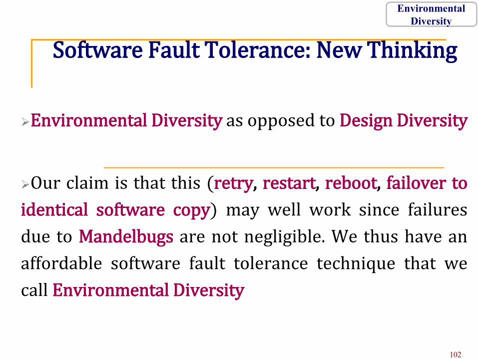
Software Fault Tolerance: New Thinking
Environmental Diversity as opposed to Design Diversity
Our claim is that this (retry, restart, reboot, failover toidentical software copy) may well work since failuresdue to Mandelbugs are not negligible. We thus have anaffordable software fault tolerance technique that wecall Environmental Diversity
102
Environmental Diversity

Back to the Availability Model
Failures
Physical failures Software failure
Power faults OS
Memory faultsNIC faults
Cooling faults
Blade faults
midplane faults
Network faults
CPU faultsbase faults
Application
I/O (RAID) faults
WAS Proxy
112 components (hardware and software)
103

Availability model of SIP on IBM WebSphere Single monolithic Markov model will have extraordinarily
large number of states – we use a multi-level approach
Subsystems modeled using Markov chains to capture dependence within
Fault tree used at higher levels as independence across subsystems can be reasonably assumed
This is an example of hierarchical composition A single monolithic model is not constructed/stored/solved Each submodel is built and solved separately and results are
propagated up to the higher-level model Our software package SHARPE facilitates such hierarchical
model composition104

Availability model of SIP on IBM WebSphere
SIP top level of the availability model
AS6
6C BSC CM1
AS5
5C BSC CM1
AS4
4B BSB CM1
AS3
3B BSB CM1
AS2
2A BSA CM1
AS1
1A BSA CM1
AS12
6F BSF CM2
AS11
3F BSF CM2
AS10
5E BSE CM2
AS9
2E BSE CM2
AS8
4D BSD CM2
AS7
1D BSD CM2
App servers
System Failure
PX1
P1 BSG CM1
PX2
P2 BSH CM2
proxy
system
k of 12
iX: ith appserver on node XPi: ith proxy serverBSX: node X hardwareCMi: chassis i hardware
105

CM
MP Cool Pwr
CM Failure
Chassis failure
BS
Base CPU Mem RAID OSeth
eth1 eth2
nic1 nic2esw1 esw2
BS Failure
Blade server failure
A circle as a leaf node is a basic eventAn inverted triangle is a shared eventA square indicates a submodel
Availability model of SIP on IBM WebSphere
Availability models of a Blade Server and Common Blade Center Hardware
106

Availability model of SIP on IBM WebSphere
Markov Availability models of subsystems
UP U1
DN
RP
cmp⋅λmp
(1-cmp)⋅λmp
αsp
µmp
αsp
midplane model Cooling subsystem model
UP U1 RP
DN
DW2λc
λc
αsp
µc
λc
µ2c
αsp
107
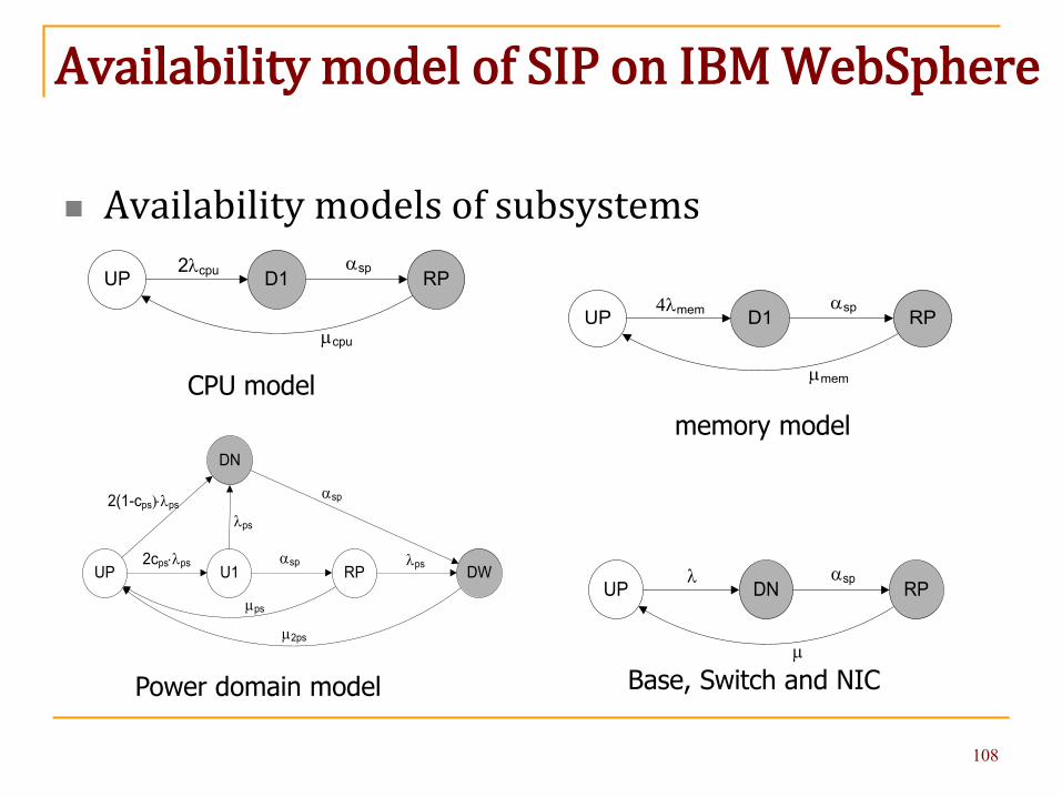
Availability model of SIP on IBM WebSphere
Availability models of subsystems
UP U1
DN
RP DW2cps⋅λps αsp
µps
λps
µ2ps
2(1-cps)⋅λpsαsp
λps
UP D1 RP2λcpu αsp
µcpu
UP D1 RP4λmem αsp
µmem
Power domain model
CPU model memory model
Base, Switch and NIC
UP DN RPλ αsp
µ
108
RAID model
OS model
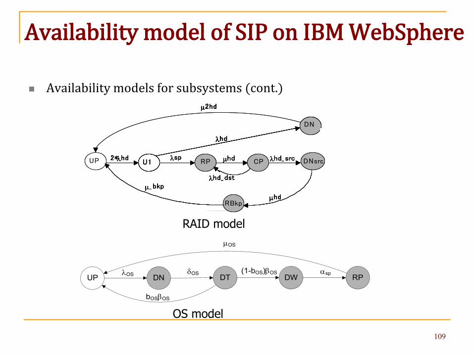
Availability model of SIP on IBM WebSphere
Availability models for subsystems (cont.)
UP DN DWλOS
µOS
RPαsp
bOSβOS
(1-bOS)βOSDT
δOS
µ2hd
UP U1 RP CP
DN
RBkp
µ_ bkp
µhd
λhd
λsp2*λhd µhd λhd_ src
λhd_ dst
DNsrc
µ2hd
UP U1 RP CP
DN
RBkp
µ_ bkp
µhd
λhd
λsp2*λhd µhd λhd_ src
λhd_ dst
DNsrc
µ2hd
UP U1 RP CP
DN
RBkp
µ_ bkp
µhd
λhd
λsp2*λhd µhd λhd_ src
λhd_ dst
DNsrc
µ2hd
UP U1 RP CP
DN
RBkp
µ_ bkp
µhd
λhd
λsp2*λhd µhd λhd_ src
λhd_ dst
DNsrc
µ2hd
UP U1 RP CP
DN
RBkp
µ_ bkp
µhd
λhd
λsp2*λhd µhd λhd_ src
λhd_ dst
DNsrc
µ2hd
UP U1 RP CP
DN
RBkp
µ_ bkp
µhd
λhd
λsp2*λhd µhd λhd_ src
λhd_ dst
DNsrc
109

Markov Availability model WebSphere AP Server
UA UR UB(1-r)ρm
rρmqρa
(1-q)ρa
bβm
RE(1-b)βm
µ
UOUPγ eδ2
1D
eδ2dδ1
(1-e)δ2
UN
δm
1N
(1-d)δ1
(1-e)δ2
2N (1-d)δ1
(1-e)δ2
eδ2 dδ1
Failure detection By WLM By Node Agent Manual detection
Recovery Node Agent
Auto process restart Manual recovery
Process restart Node reboot Repair
• Application server and proxy server (with escalated levels of recovery)• Delay and imperfect coverage in each step of recovery modeled• Use of restart, failover to an identical replica or reboot as a method of
recovery after a software failure
110

Hierarchical Composition
CM
MP Cool Pwr
CM Failure
BS
Base CPU Mem RAID OSeth
eth1 eth2
nic1 nic2esw1 esw2
BS Failure
UA UR UB(1-r)ρm
rρmqρa
(1-q)ρa
bβm
RE(1-b)βm
µ
UOUPγ eδ2
1D
eδ2dδ1
(1-e)δ2
UN
δm
1N
(1-d)δ1
(1-e)δ2
2N (1-d)δ1
(1-e)δ2
eδ2 dδ1
UP U1
DN
RP DW2cps⋅λps αsp
µps
λps
µ2ps
2(1-cps)⋅λpsαsp
λps
AS6
6C BS C CM 1
AS 5
5C BS C CM 1
AS 4
4B BS B CM 1
AS 3
3B BS B CM 1
AS2
2A BS A CM 1
AS1
1A BS A CM 1
AS 12
6F BS F CM 2
AS 11
3F BS F CM 2
AS 10
5E BS E CM 2
AS9
2E BS E CM 2
AS 8
4D BS D CM 2
AS7
1D BS D CM 2
App servers
System Failure
PX1
P1 BS G CM 1
PX 2
P2 BS H CM 2
proxy
system
k of 12 AS1
1A BSA CM1
A single monolithic Markov model will have too many states
111

Model Parameterization Types of parameters
Hardware component failure rates Software component failure rates Detection, restart, reboot, repair delays Imperfect coverages for each of the above recovery phases
The parameter values obtained from Field data for hardware component failure rates High availability testing for detection/restart/reboot delays Agreed upon assumptions for other parameters
Uncertainty in parameter values (assumed value or based on limited test data) Sensitivity analysis w.r.t. that parameter performed
112

Para
met
ers f
or th
e H
ardw
are
Com
pone
nts
113

Para
met
ers f
or th
e so
ftw
are
com
pone
nts
114

System and subsystem downtime (min/year)
115
Downtime at different levels of AS redundancy (k-1) Downtime of individual components

Availability model of SIP on IBM WebSphere (contributions)
Developed a very comprehensive availability model Hardware and software failures Hardware and Software failure-detection delays Software Failover delay Escalated levels of recovery
Automated and manual restart, reboot, repair Imperfect coverage (detection, failover, restart, reboot)
Many of the parameters collected from experiments, some obtained from tables; few of them assumed
Detailed sensitivity analysis to find bottlenecks and give feedback to designers
Developed a new method for calculating DPM (defects per million) Taking into account interaction between call flow and failure/recovery Retry of messages (this model will be published in the future)
This model was responsible for the sale of the system by IBM
116

Import graph for SIP Availability Model
117

Hierarchical Composition
Many more examples of such models can be found in the book (Trivedi & Bobbio, Reliability and Availability: Modeling, Analysis, Applications, Cambridge University Press, 2017) and other papers Availability Models Reliability Models Performance Models Performability Models Survivability Models Dynamic Fault Tree Models
118

Hierarchical Composition Matrix-Level vs. Model-Level vs. System-Level Decomposition Multi-level modeling formalism -- meta-modeling language? What kinds of quantities to pass between sub-models? Exact vs. approximate solution If approximate, bounding/estimating errors of approximation? Import graph
Acyclic Cyclic Fixed-point iteration
119

Analytic Modeling Taxonomy
Hierarchical modelsLargeness avoidance
Analytic models
Combinatorial modelsEfficiency, simplicity
State-space modelsDependency capture
Fixed point iterationNearly independent
120

Return to the SIP Availability Model
We ignored one dependence assuming its effect will be negligible
Two App servers share a blade server node
121

Architecture of SIP on IBM WebSphere
Replication domain Nodes
1 A, D2 A, E3 B, F4 B, D5 C, E6 C, F
AS: WebSphere Appl. Server (WAS)
122

Return to the SIP Availability Model
Two App servers share a blade server node If one App server needs reboot its OS or
repair of the blade is needed, it affects the other app server on the same blade – a forced dependence
We ignored this dependence earlier We now account for this dependence
123

Two app server CTMCs run nearly independently
124

Two app server CTMCs run nearly independently
But need to be synchronized at state UBsince when one app server needs to be rebooted, the other is forced to be rebooted
Similarly the two need to be synchronized at states RE since when one app server blade needed to be repaired, the other is to repair
Need to combine the two CTMCs
125

Two Synchronized app servers
Combined Markov model (CTMC) is too large to construct by hand.
We use a high-level formalism of stochastic Petri net (the flavor known as stochastic reward net (SRN)).
SRNs extend other SPN formalisms by adding variable cardinality arcs, transition priorities, guard functions and the ability to specify reward rates at the net level
SRN models can be automatically converted into underlying Markov (reward) model and solved for the measures of interest such as DT (downtime) and many more
126

In order to model the synchronization
We use an SRN model to show two synchronized CTMCs and solve the SRN model using SHARPE software package
We start by first converting single app server CTMC to an SRN
127
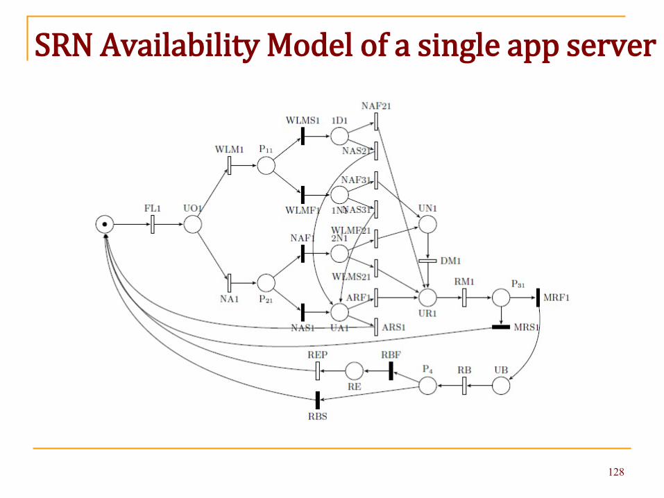
SRN Availability Model of a single app server
128

In order to model the synchronization
We use an SRN model to show two synchronized CTMCs and solve the SRN model using SHARPE
Dotted arcs are variable cardinality arcs that flush the places of any token they may have
129

SRN Availability Model of two synchronized app servers
130

Two synchronized app servers model
131
We used an SRN model to capture two synchronized CTMCs and solve the SRN model using SHARPE
Underlying reachability graph has 65 vanishing markings and 66 tangible markings – so the CTMC generated from this SRN has 66 states
Note that if two CTMCs were independent then the combined composed CTMC will have the cross-product state space with 10*10=100 states
But 8 out of 10 states of each CTMC are independent while 2 states are common or shared states. Hence the resulting number of states is 8*8+2=66

CTMC approximation
132
Then we develop a simple approximate CTMC in which we have added a transition (shown as dotted arcs) from each of the states, UP, UO, 1N, 2N, 1D, UA, UN and UR to state UB at rate x as shown in the next slide
Now each app server CTMC model can be considered independent for the overall SIP availability model

Modified CTMC to account for forced reboot
133

Fixed-Point Iteration
134
Since x is an input parameter for the CTMC, πUR is a function of x, thus, we have a fixed-point problem:
Rate x= πUR (x)*(1-r) * ϱm
We initialize x so that x0=0.0001*(1-r) * ϱm
We solve iteratively using successive substitution: xi+1= πUR (xi)*(1-r) * ϱm

Fixed-Point Iteration
135
It took only 3 iterations to converge to a fixed point
App server steady state availability computed with the exact composed CTMC and with the fixed-point iteration approximation are both 0.999844145
The effect of this dependency is negligible as the steady state availability of the app server without the dependence is 0.999845429 while with the dependence it is 0.999844145

Scalable Model for IaaS Cloud Availability and Downtime
Ref: Ghosh, Longo, Frattini, Russo, Trivedi,“Scalable Analytics for IaaS Cloud Availability,”
IEEE Trans. Cloud Comput., 2014
136

Monolithic SRN Model
137

Monolithic ModelMonolithic SRN model is automatically translated into CTMC or Markov Reward ModelHowever the model not scalable as state-space size of this model is extremely large
#PMs per pool #states #non-zero matrix entries
3 10, 272 59, 560
4 67,075 453, 970
5 334,948 2, 526, 920
6 1,371,436 11, 220, 964
7 4,816,252 41, 980, 324
8 Memory overflow Memory overflow
10 - -
138

Decompose into Interacting Sub-models
SRN sub-model for hot pool
SRN sub-model for warm poolSRN sub-model for cold pool
139

Import graph and model outputs
Model outputs: mean number of PMs in each pool (E[#Ph], E[#Pw], and E[#Pc]) Downtime in minutes per year
140

Many questions
Existence of Fixed Point (easy): IEEE TCC 2014 (In a more general setting: Mainkar & Trivedi paper in IEEE-TSE, 1996)
Uniqueness (some cases) Rate of convergence Accuracy Scalability
141

Monolithic vs. interacting sub-models
#states, #non-zero entries
142
Steps for system availability modeling
List all possible component level failures (hardware, software) List of all failure detectors & match with failure types List all recovery mechanisms & match with failure types Allocation of software modules to hardware units Formulate the model Face validation and verification of the model Parameterization of the model (tables, websites, experiments) Solve the model (using SHARPE, SPNP or similar software
packages) to detect bottlenecks, sensitivity analysis, suggest parameters to be monitored more accurately
What-if analysis to suggest improvements Validate the model
143

Outline
Introduction and Motivation Reliability and Availability Models Conclusions References
144
System Reliability/Availability Models
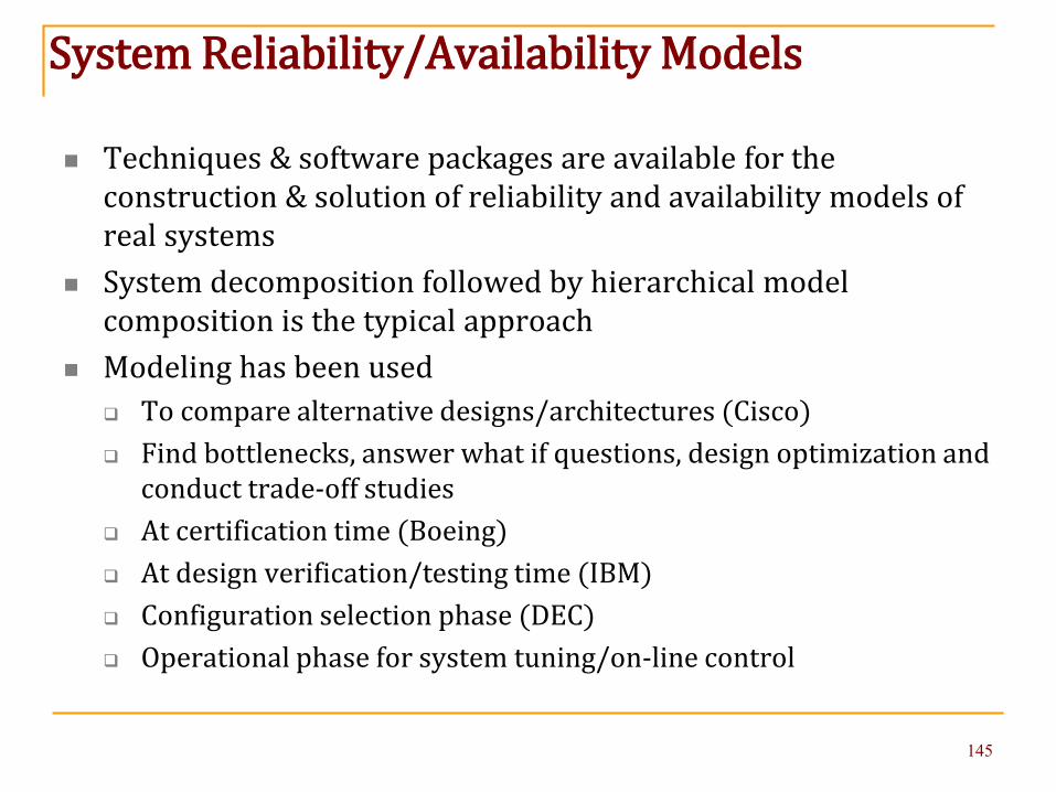
Techniques & software packages are available for the construction & solution of reliability and availability models of real systems
System decomposition followed by hierarchical model composition is the typical approach
Modeling has been used To compare alternative designs/architectures (Cisco) Find bottlenecks, answer what if questions, design optimization and
conduct trade-off studies At certification time (Boeing) At design verification/testing time (IBM) Configuration selection phase (DEC) Operational phase for system tuning/on-line control
145

System Reliability/Availability Models Model Types in Use
Non-state-Space: Reliability Block Diagram, Fault tree, Reliability graph
State-space: Markov models & stochastic Petri nets, Semi-Markov, Markov regenerative and non-homogeneous Markov models
Hierarchical composition Top level is usually an RBD or a fault tree Bottom level models are usually Markov chains
Fixed-point iterative Solution types
Analytic closed-form Analytic numerical (using a software package) Simulative
Software packages SHARPE or similar tools are used to construct and solve such models
Structural as well as parametric assumptions means that numbers produced should be taken with a grain of salt
146
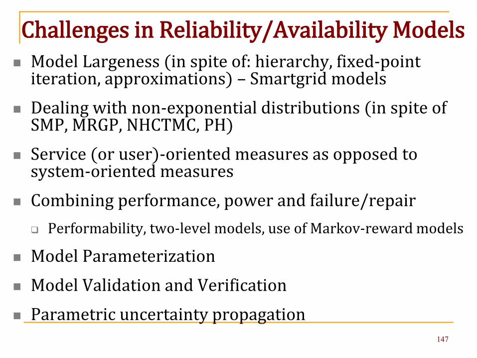
Challenges in Reliability/Availability Models Model Largeness (in spite of: hierarchy, fixed-point
iteration, approximations) – Smartgrid models Dealing with non-exponential distributions (in spite of
SMP, MRGP, NHCTMC, PH) Service (or user)-oriented measures as opposed to
system-oriented measures Combining performance, power and failure/repair
Performability, two-level models, use of Markov-reward models
Model Parameterization Model Validation and Verification Parametric uncertainty propagation
147

Challenges in Reliability/Availability Models
Model Verification and Validation Verification checked by someone else, check logical flows, cross-check using alternative solutions (e.g. alternative
analytic/simulation) Validation Face validation, Input-Output validation, Validation of model assumptions
148

Model Parameterization Hardware/Software Configuration parameters Hardware component MTTFs Software component MTTFs
OS, IBM Application, customer software, third party Hardware/Software Failover times Restart/Reboot times Coverage (Success) probabilities
Detection, location, restart, reconfiguration, repair Repair time
Hot swap, multiple component at once, DOA (dead on arrival), shared/not shared, field service travel time, preventive vs. corrective
Uncertainty propagation: Dealing with not only Aleatory (built into the system models) but also epistemic (parametric) uncertainty
149

Message to Young Researchers Pick a real problem rather than one from literature
whenever possible There should be plenty of real problems in Industry Keep an open mind Ask questions and Listen carefully
It is possible to write scholarly articles based on work done on real problems
Use software packages [e.g., SHARPE, SPNP] whenever applicable [as opposed writing your own code to generate and solve models]
150

Outline of the book: Reliability and Availability Engineering
Part I – Introduction (Chapters 1:3)
Part II - Non-state-space models (Chapters 4:8)
Part III - State-space Models with Exponential Distributions (Chapters 9:12)
Part IV - State-space Models with Non-Exponential Distributions (Chapters 13:15)
Part V - Multi-Level Models (Chapters 16:17)
Part VI - Case Studies (Chapter 18)
151

Outline of the book: Reliability and Availability Engineering
152

Outline
Introduction and Motivation Reliability and Availability Models Conclusions References
153

Selected References Trivedi, Probability and Statistics with Reliability, Queuing, and Computer Science
Applications. John Wiley, 2nd edition, 2001; revised paperback, 2016 Tomek & Trivedi, Fixed-Point Iteration in Availability Modeling, Informatik-Fachberichte, Dal
Cin (ed.), Springer-Verlag, Berlin, 1991 Mainkar & Trivedi, Sufficient Conditions for Existence of a Fixed Point in Stochastic Reward
Net-Based Iterative Models, IEEE TSE, 1996 Trivedi, Vasireddy, Trindade, Nathan, Castro, “Modeling High Availability Systems,” PRDC
2006 Trivedi & Bobbio, Reliability and Availability: Modeling, Analysis, Applications, Cambridge
University Press, 2017 Trivedi, Wang, Hunt, Rindos, Smith, Vashaw, “Availability Modeling of SIP Protocol on IBM
WebSphere,” PRDC 2008 Smith, Trivedi, Tomek, Ackaret, Availability analysis of blade server systems, IBM Sys. J., 2008. Trivedi & Sahner, SHARPE at the Age of Twenty two, ACM SIGMETRICS, Performance
Evaluation Review, 2008 Trivedi, Wang & Hunt. “Computing the number of calls dropped due to failures,” ISSRE2010 Mishra, Trivedi & Some. "Uncertainty Analysis of the Remote Exploration and
Experimentation System", AIAA Journal of Spacecraft and Rockets, 2012 Ghosh, Longo, Frattini, Russo & Trivedi, “Scalable Analytics for IaaS Cloud Availability”, IEEE
Trans. on Cloud Computing, 2014 Malhotra, Trivedi, “Power-Hierarchy of Dependability -Model Types,” IEEE-TR, 1994
154

Thank you!
155

Contact Information and more sources
Kishor Trivedi: [email protected]/profile/Kishor_Trivedi2
Andrea Bobbio: [email protected]
156