release 0.0.0 matthew vernacchia

proptools DocumentationRelease 0.0.0

Matthew Vernacchia

Sep 22, 2019

Contents

1 Tutorials 31.1 Nozzle Flow . . . . . . . . . . . . . . . . . . . . . . . . . . . . . . . . . . . . . . . . . . . . . . . 31.2 Solid-Propellant Rocket Motors . . . . . . . . . . . . . . . . . . . . . . . . . . . . . . . . . . . . . 191.3 Electric Propulsion Basics . . . . . . . . . . . . . . . . . . . . . . . . . . . . . . . . . . . . . . . . 29

2 Package contents 352.1 proptools . . . . . . . . . . . . . . . . . . . . . . . . . . . . . . . . . . . . . . . . . . . . . . . . . 35

Bibliography 59

Python Module Index 61

Index 63

i

proptools Documentation, Release 0.0.0

Proptools is a Python package for preliminary design of rocket propulsion systems.

Proptools provides implementations of equations for nozzle flow, turbo-machinery and rocket structures. The projectaims to cover most of the commonly used equations in Rocket Propulsion Elements by George Sutton and OscarBiblarz and Modern Engineering for Design of Liquid-Propellant Rocket Engines by Dieter Huzel and David Huang.

Proptools can be used as a desktop calculator:

>> from proptools import nozzle>> p_c = 10e6; p_e = 100e3; gamma = 1.2; m_molar = 20e-3; T_c = 3000.>> C_f = nozzle.thrust_coef(p_c, p_e, gamma)>> c_star = nozzle.c_star(gamma, m_molar, T_c)>> I_sp = C_f * c_star / nozzle.g>> print "The engine's ideal sea level specific impulse is {:.1f} seconds.".format(I_→˓sp)The engine's ideal sea level specific impulse is 288.7 seconds.

Proptools can also be used as a library in other propulsion design and analysis software. It is distributed under a MITLicense and can be used in commercial projects.

Contents 1

https://github.com/mvernacc/proptools/blob/master/LICENSE

https://github.com/mvernacc/proptools/blob/master/LICENSE


2 Contents

CHAPTER 1

Tutorials

1.1 Nozzle Flow

Nozzle flow theory can predict the thrust and specific impulse of a rocket engine. The following example predicts theperformance of an engine which operates at chamber pressure of 10 MPa, chamber temperature of 3000 K, and has100 mm diameter nozzle throat.

"""Estimate specific impulse, thrust and mass flow."""from math import pifrom proptools import nozzle

# Declare engine design parametersp_c = 10e6 # Chamber pressure [units: pascal]p_e = 100e3 # Exit pressure [units: pascal]gamma = 1.2 # Exhaust heat capacity ratio [units: dimensionless]m_molar = 20e-3 # Exhaust molar mass [units: kilogram mole**1]T_c = 3000. # Chamber temperature [units: kelvin]A_t = pi * (0.1 / 2)**2 # Throat area [units: meter**2]

# Predict engine performanceC_f = nozzle.thrust_coef(p_c, p_e, gamma) # Thrust coefficient [units:→˓dimensionless]c_star = nozzle.c_star(gamma, m_molar, T_c) # Characteristic velocity [units:→˓meter second**-1]I_sp = C_f * c_star / nozzle.g # Specific impulse [units: second]F = A_t * p_c * C_f # Thrust [units: newton]m_dot = A_t * p_c / c_star # Propellant mass flow [units: kilogram second**-1]

print 'Specific impulse = {:.1f} s'.format(I_sp)print 'Thrust = {:.1f} kN'.format(F * 1e-3)print 'Mass flow = {:.1f} kg s**-1'.format(m_dot)

Output:

3


Specific impulse = 288.7 s

Thrust = 129.2 kN

Mass flow = 45.6 kg s**-1

The rest of this page derives the nozzle flow theory, and demonstrates other features of proptools.nozzle.

1.1.1 Ideal Nozzle Flow

The purpose of a rocket is to generate thrust by expelling mass at high velocity. The rocket nozzle is a flow devicewhich accelerates gas to high velocity before it is expelled from the vehicle. The nozzle accelerates the gas byconverting some of the gas’s thermal energy into kinetic energy.

Ideal nozzle flow is a simplified model of the aero- and thermo-dynamic behavior of fluid in a nozzle. The idealmodel allows us to write algebraic relations between an engine’s geometry and operating conditions (e.g. throat area,chamber pressure, chamber temperature) and its performance (e.g. thrust and specific impulse). These equations arefundamental tools for the preliminary design of rocket propulsion systems.

The assumptions of the ideal model are:

1. The fluid flowing through the nozzle is gaseous.

2. The gas is homogeneous, obeys the ideal gas law, and is calorically perfect. Its molar mass (ℳ) and heatcapacities (𝑐𝑝, 𝑐𝑣) are constant throughout the fluid, and do not vary with temperature.

3. There is no heat transfer to or from the gas. Therefore, the flow is adiabatic. The specific enthalpy ℎ is constantthroughout the nozzle.

4. There are no viscous effects or shocks within the gas or at its boundaries. Therefore, the flow is reversible. Ifthe flow is both adiabatic and reversible, it is isentropic: the specific entropy 𝑠 is constant throughout the nozzle.

5. The flow is steady; 𝑑𝑑𝑡 = 0.

6. The flow is quasi one dimensional. The flow state varies only in the axial direction of the nozzle.

7. The flow velocity is axially directed.

8. The flow does not react in the nozzle. The chemical equilibrium established in the combustion chamber doesnot change as the gas flows through the nozzle. This assumption is known as “frozen flow”.

These assumptions are usually acceptably accurate for preliminary design work. Most rocket engines perform within1% to 6% of the ideal model predictions [RPE].

1.1.2 Isentropic Relations

Under the assumption of isentropic flow and calorically perfect gas, there are several useful relations between fluidstates. These relations depend on the heat capacity ratio, 𝛾 = 𝑐𝑝/𝑐𝑣 . Consider two gas states, 1 and 2, which areisentropically related (𝑠1 = 𝑠2). The states’ pressure, temperature and density ratios are related:

𝑝1𝑝2

=

(︂𝜌1𝜌2

)︂𝛾

=

(︂𝑇1

𝑇2

)︂ 𝛾𝛾−1

4 Chapter 1. Tutorials


Stagnation state

Now consider the relation between static and stagnation states in a moving fluid. The stagnation state is the state amoving fluid would reach if it were isentropically decelerated to zero velocity. The stagnation enthalpy ℎ0 is the sumof the static enthalpy and the specific kinetic energy:

ℎ0 = ℎ +1

2𝑣2

For a calorically perfect gas, 𝑇 = ℎ/𝑐𝑝, and the stagnation temperature is:

𝑇0 = 𝑇 +𝑣2

2𝑐𝑝

It is helpful to write the fluid properties in terms of the Mach number 𝑀 , instead of the velocity. Mach number is thevelocity normalized by the local speed of sound, 𝑎 =

√𝛾𝑅𝑇 . In terms of Mach number, the stagnation temperature

is:

𝑇0 = 𝑇

(︂1 +

𝛾 − 1

2𝑀2

)︂Because the static and stagnation states are isentropically related, 𝑝0

𝑝 =(︀𝑇0

𝑇

)︀ 𝛾𝛾−1 . Therefore, the stagnation pressure

is:

𝑝0 = 𝑝

(︂1 +

𝛾 − 1

2𝑀2

)︂ 𝛾𝛾−1

Use proptools to plot the stagnation state variables against Mach number:

"""Plot isentropic relations."""import numpy as npfrom matplotlib import pyplot as pltfrom proptools import isentropic

M = np.logspace(-1, 1)gamma = 1.2

plt.loglog(M, 1 / isentropic.stag_temperature_ratio(M, gamma), label='$T / T_0$')plt.loglog(M, 1 / isentropic.stag_pressure_ratio(M, gamma), label='$p / p_0$')plt.loglog(M, 1 / isentropic.stag_density_ratio(M, gamma), label='$\\rho / \\rho_0$')plt.xlabel('Mach number [-]')plt.ylabel('Static / stagnation [-]')plt.title('Isentropic flow relations for $\gamma={:.2f}$'.format(gamma))plt.xlim(0.1, 10)plt.ylim([1e-3, 1.1])plt.axvline(x=1, color='grey', linestyle=':')plt.legend(loc='lower left')plt.show()

Exit velocity

The exit velocity of the exhaust gas is the fundamental measure of efficiency for rocket propulsion systems, as therocket equation shows. We can now show a basic relation between the exit velocity and the combustion conditions ofthe rocket. First, use the conservation of energy to relate the velocity at any two points in the flow:

𝑣2 =√︁

2(ℎ1 − ℎ2) + 𝑣21

1.1. Nozzle Flow 5

https://en.wikipedia.org/wiki/Tsiolkovsky_rocket_equation


10 1 100 101

Mach number [-]

10 3

10 2

10 1

100

Stat

ic / s

tagn

atio

n [-]

Isentropic flow relations for = 1.20

T/T0p/p0/ 0



We can replace the enthalpy difference with an expression of the pressures and temperatures, using the isentropicrelations.

𝑣2 =

⎯⎸⎸⎷ 2𝛾

𝛾 − 1𝑅𝑇1

(︃1 −

(︂𝑝2𝑝1

)︂ 𝛾−1𝛾

)︃+ 𝑣21

Set state 1 to be the conditions in the combustion chamber: 𝑇1 = 𝑇𝑐, 𝑝1 = 𝑝𝑐, 𝑣1 ≈ 0. Set state 2 to be the state at thenozzle exit: 𝑝2 = 𝑝𝑒, 𝑣2 = 𝑣𝑒. This gives the exit velocity:

𝑣𝑒 =

⎯⎸⎸⎷ 2𝛾

𝛾 − 1𝑅𝑇𝑐

(︃1 −

(︂𝑝𝑒𝑝𝑐

)︂ 𝛾−1𝛾

)︃

=

⎯⎸⎸⎷ 2𝛾

𝛾 − 1ℛ 𝑇𝑐

ℳ

(︃1 −


)︂ 𝛾−1𝛾

)︃

where ℛ = 8.314 J mol -1 K -1 is the universal gas constant and ℳ is the molar mass of the exhaust gas. Temperatureand molar mass have the most significant effect on exit velocity. To maximize exit velocity, a rocket should burn pro-pellants which yield a high flame temperature and low molar mass exhaust. This is why many rockets burn hydrogenand oxygen: they yield a high flame temperature, and the exhaust (mostly H2 and H2O) is of low molar mass.

The pressure ratio 𝑝𝑒/𝑝𝑐 is usually quite small. As the pressure ratio goes to zero, the exit vleocity approaches itsmaximum for a given 𝑇𝑐,ℳ and 𝛾.

𝑝𝑒𝑝𝑐

→ 0 ⇒ 1 −(︂𝑝𝑒𝑝𝑐

)︂ 𝛾−1𝛾

→ 1

If 𝑝𝑒 ≪ 𝑝𝑐, the pressures have a weak effect on exit velocity.

The heat capacity ratio 𝛾 has a weak effect on exit velocity. Decreasing 𝛾 increases exit velocity.

Use proptools to find the exit velocity of the example engine:

"""Estimate exit velocity."""from proptools import isentropic

# Declare engine design parametersp_c = 10e6 # Chamber pressure [units: pascal]p_e = 100e3 # Exit pressure [units: pascal]gamma = 1.2 # Exhaust heat capacity ratio [units: dimensionless]m_molar = 20e-3 # Exhaust molar mass [units: kilogram mole**1]T_c = 3000. # Chamber temperature [units: kelvin]

# Compute the exit velocityv_e = isentropic.velocity(v_1=0, p_1=p_c, T_1=T_c, p_2=p_e, gamma=gamma, m_molar=m_→˓molar)

print 'Exit velocity = {:.0f} m s**-1'.format(v_e)

Exit velocity = 2832 m s**-1

1.1.3 Mach-Area Relation

Using the isentropic relations, we can find how the Mach number of the flow varies with the cross sectional area of thenozzle. This allows the design of a nozzle geometry which will accelerate the flow the high speeds needed for rocketpropulsion.

1.1. Nozzle Flow 7


Start with the conservation of mass. Because the flow is quasi- one dimensional, the mass flow through every cross-section of the nozzle must be the same:

�̇� = 𝐴𝑣𝜌 = const

where 𝐴 is the cross-sectional area of the nozzle flow passage (normal to the flow axis). To conserve mass, the ratioof areas between any two points along the nozzle axis must be:

𝐴1

𝐴2=

𝑣2𝜌2𝑣1𝜌1

Use the isentropic relations to write the velocity and density in terms of Mach number, and simplify:

𝐴1

𝐴2=

𝑀2

𝑀1

(︃1 + 𝛾−1

2 𝑀21

1 + 𝛾−12 𝑀2

2

)︃ 𝛾+12(𝛾−1)

We can use proptools to plot Mach-Area relation. Let 𝑀2 = 1 and plot 𝐴1/𝐴2 vs 𝑀1:

"""Plot the Mach-Area relation."""import numpy as npfrom matplotlib import pyplot as pltfrom proptools import nozzle

M_1 = np.linspace(0.1, 10) # Mach number [units: dimensionless]gamma = 1.2 # Exhaust heat capacity ratio [units: dimensionless]

area_ratio = nozzle.area_from_mach(M_1, gamma)

plt.loglog(M_1, area_ratio)plt.xlabel('Mach number $M_1$ [-]')plt.ylabel('Area ratio $A_1 / A_2$ [-]')plt.title('Mach-Area relation for $M_2 = 1$')plt.ylim([1, 1e3])plt.show()

We see that the nozzle area has a minimum at 𝑀 = 1. At subsonic speeds, Mach number increases as the area isdecreased. At supersonic speeds (𝑀 > 1), Mach number increases as area increases. For a flow passage to accelerategas from subsonic to supersonic speeds, it must first decrease in area, then increase in area. Therefore, most rocketnozzles have a convergent-divergent shape. Larger expansions of the divergent section lead to higher exit Machnumbers.

1.1.4 Choked Flow

The station of minimum area in a converging-diverging nozzle is known as the nozzle throat. If the pressure ratioacross the nozzle is at least:

𝑝𝑐𝑝𝑒

>

(︂𝛾 + 1

2

)︂ 𝛾𝛾−1

∼ 1.8

then the flow at the throat will be sonic (𝑀 = 1) and the flow in the diverging section will be supersonic. The velocityat the throat is:

𝑣𝑡 =√︀𝛾𝑅𝑇𝑡 =

√︂2𝛾

𝛾 + 1𝑅𝑇𝑐

The mass flow at the sonic throat (i.e. through the nozzle) is:

�̇� = 𝐴𝑡𝑣𝑡𝜌𝑡 = 𝐴𝑡𝑝𝑐𝛾√𝛾𝑅𝑇𝑐

(︂2

𝛾 + 1

)︂ 𝛾+12(𝛾−1)



10 1 100 101

Mach number M1 [-]

100

101

102

103

Area

ratio

A1/A

2 [-]

Mach-Area relation for M2 = 1

1.1. Nozzle Flow 9


Fig. 1: The typical converging-diverging shape of rocket nozzles is shown in this cutaway of the Thiokol C-1 engine.Image credit: Smithsonian Institution, National Air and Space Museum


https://airandspace.si.edu/collection-objects/rocket-engine-liquid-fuel-radiamic-cutaway-also-designated-c-1


Notice that the mass flow does not depend on the exit pressure. If the exit pressure is sufficiently low to produce sonicflow at the throat, the nozzle is choked and further decreases in exit pressure will not alter the mass flow. Increasingthe chamber pressure increases the density at the throat, and therefore will increase the mass flow which can “fitthrough” the throat. Increasing the chamber temperature increases the throat velocity but decreases the density by alarger amount; the net effect is to decrease mass flow as 1/

√𝑇𝑐.

Use proptools to compute the mass flow of the example engine:

"""Check that the nozzle is choked and find the mass flow."""from math import pifrom proptools import nozzle

# Declare engine design parametersp_c = 10e6 # Chamber pressure [units: pascal]p_e = 100e3 # Exit pressure [units: pascal]gamma = 1.2 # Exhaust heat capacity ratio [units: dimensionless]m_molar = 20e-3 # Exhaust molar mass [units: kilogram mole**1]T_c = 3000. # Chamber temperature [units: kelvin]A_t = pi * (0.1 / 2)**2 # Throat area [units: meter**2]

# Check chokingif nozzle.is_choked(p_c, p_e, gamma):

print 'The flow is choked'

# Compute the mass flow [units: kilogram second**-1]m_dot = nozzle.mass_flow(A_t, p_c, T_c, gamma, m_molar)

print 'Mass flow = {:.1f} kg s**-1'.format(m_dot)

The flow is choked

Mass flow = 45.6 kg s**-1

1.1.5 Thrust

The thrust force of a rocket engine is equal to the momentum flow out of the nozzle plus a pressure force at the nozzleexit:

𝐹 = �̇�𝑣𝑒 + (𝑝𝑒 − 𝑝𝑎)𝐴𝑒

where 𝑝𝑎 is the ambient pressure and 𝐴𝑒 is the nozzle exit area. We can rewrite this in terms of the chamber pressure:

𝐹 = 𝐴𝑡𝑝𝑐

⎯⎸⎸⎷ 2𝛾2

𝛾 − 1

(︂2

𝛾 + 1

)︂ 𝛾+1𝛾−1

(︃1 −


)︂ 𝛾−1𝛾

)︃+ (𝑝𝑒 − 𝑝𝑎)𝐴𝑒

Note that thrust depends only on 𝛾 and the nozzle pressures and areas; not chamber temperature.

Use proptools to plot thrust versus chamber pressure for the example engine:

"""Plot thrust vs chmaber pressure."""

import numpy as npfrom matplotlib import pyplot as pltfrom proptools import nozzle

(continues on next page)

1.1. Nozzle Flow 11


(continued from previous page)

p_c = np.linspace(1e6, 20e6) # Chamber pressure [units: pascal]p_e = 100e3 # Exit pressure [units: pascal]p_a = 100e3 # Ambient pressure [units: pascal]gamma = 1.2 # Exhaust heat capacity ratio [units: dimensionless]A_t = np.pi * (0.1 / 2)**2 # Throat area [units: meter**2]

# Compute thrust [units: newton]F = nozzle.thrust(A_t, p_c, p_e, gamma)

plt.plot(p_c * 1e-6, F * 1e-3)plt.xlabel('Chamber pressure $p_c$ [MPa]')plt.ylabel('Thrust $F$ [kN]')plt.title('Thrust vs chamber pressure at $p_e = p_a = {:.0f}$ kPa'.format(p_e * 1e-3))plt.show()

2.5 5.0 7.5 10.0 12.5 15.0 17.5 20.0Chamber pressure pc [MPa]

0

50

100

150

200

250

Thru

st F

[kN]

Thrust vs chamber pressure at pe = pa = 100 kPa

Note that thrust is almost linear in chamber pressure.

We can also explore the variation of thrust with ambient pressure for fixed 𝑝𝑐, 𝑝𝑒:

"""Plot thrust vs ambient pressure."""import numpy as npfrom matplotlib import pyplot as pltimport skaero.atmosphere.coesa as atmo





from proptools import nozzle

p_c = 10e6 # Chamber pressure [units: pascal]p_e = 100e3 # Exit pressure [units: pascal]p_a = np.linspace(0, 100e3) # Ambient pressure [units: pascal]gamma = 1.2 # Exhaust heat capacity ratio [units: dimensionless]A_t = np.pi * (0.1 / 2)**2 # Throat area [units: meter**2]

# Compute thrust [units: newton]F = nozzle.thrust(A_t, p_c, p_e, gamma,

p_a=p_a, er=nozzle.er_from_p(p_c, p_e, gamma))

ax1 = plt.subplot(111)plt.plot(p_a * 1e-3, F * 1e-3)plt.xlabel('Ambient pressure $p_a$ [kPa]')plt.ylabel('Thrust $F$ [kN]')plt.suptitle('Thrust vs ambient pressure at $p_c = {:.0f}$ MPa, $p_e = {:.0f}$ kPa'.→˓format(

p_c *1e-6, p_e * 1e-3))

# Add altitude on second axisylim = plt.ylim()ax2 = ax1.twiny()new_tick_locations = np.array([100, 75, 50, 25, 1])ax2.set_xlim(ax1.get_xlim())ax2.set_xticks(new_tick_locations)

def tick_function(p):"""Map atmospheric pressure [units: kilopascal] to altitude [units: kilometer]."""h_table = np.linspace(84e3, 0) # altitude [units: meter]p_table = atmo.pressure(h_table) # atmo pressure [units: pascal]return np.interp(p * 1e3, p_table, h_table) * 1e-3

ax2.set_xticklabels(['{:.0f}'.format(h) for h in tick_function(new_tick_locations)])ax2.set_xlabel('Altitude [km]')ax2.tick_params(axis='y', direction='in', pad=-25)plt.subplots_adjust(top=0.8)plt.show()

1.1.6 Thrust coefficient

We can normalize thrust by 𝐴𝑡𝑝𝑐 to give a non-dimensional measure of nozzle efficiency, which is independent ofengine size or power level. This is the thrust coefficient, 𝐶𝐹 :

𝐶𝐹 ≡ 𝐹

𝐴𝑡𝑝𝑐

For an ideal nozzle, the thrust coefficient is:

𝐶𝐹 =

⎯⎸⎸⎷ 2𝛾2

𝛾 − 1

(︂2

𝛾 + 1

)︂ 𝛾+1𝛾−1

(︃1 −


)︂ 𝛾−1𝛾

)︃+

𝑝𝑒 − 𝑝𝑎𝑝𝑐

𝐴𝑒

𝐴𝑡

Note that 𝐶𝐹 is independent of the combustion temperature or the engine size. It depends only on the heat capacityratio, nozzle pressures, and expansion ratio (𝐴𝑒/𝐴𝑡). Therefore, 𝐶𝐹 is a figure of merit for the nozzle expansion

1.1. Nozzle Flow 13


process. It can be used to compare the efficiency of different nozzle designs on different engines. Values of 𝐶𝐹 aregenerally between 0.8 and 2.2, with higher values indicating better nozzle performance.

1.1.7 Expansion Ratio

The expansion ratio is an important design parameter which affects nozzle efficiency. It is the ratio of exit area tothroat area:

𝜖 ≡ 𝐴𝑒

𝐴𝑡

The expansion ratio appears directly in the equation for thrust coefficient. The expansion ratio also allows the nozzledesigner to set the exit pressure. The relation between expansion ratio and pressure ratio can be found from massconservation and the isentropic relations:

𝜖 =𝐴𝑒

𝐴𝑡=

𝜌𝑡𝑣𝑡𝜌𝑒𝑣𝑒

=

⎛⎝(︂𝛾 + 1

2

)︂ 1𝛾−1


)︂ 1𝛾

⎯⎸⎸⎷𝛾 + 1

𝛾 − 1

(︃1 −


)︂ 𝛾−1𝛾

)︃⎞⎠−1

This relation is implemented in proptools:

"""Compute the expansion ratio for a given pressure ratio."""from proptools import nozzle

p_c = 10e6 # Chamber pressure [units: pascal]p_e = 100e3 # Exit pressure [units: pascal]gamma = 1.2 # Exhaust heat capacity ratio [units: dimensionless]

# Solve for the expansion ratio [units: dimensionless]exp_ratio = nozzle.er_from_p(p_c, p_e, gamma)

print 'Expansion ratio = {:.1f}'.format(exp_ratio)

Expansion ratio = 11.9

We can also solve the inverse problem:

"""Compute the pressure ratio from a given expansion ratio."""from scipy.optimize import fsolvefrom proptools import nozzle

p_c = 10e6 # Chamber pressure [units: pascal]gamma = 1.2 # Exhaust heat capacity ratio [units: dimensionless]exp_ratio = 11.9 # Expansion ratio [units: dimensionless]

# Solve for the exit pressure [units: pascal].p_e = p_c * nozzle.pressure_from_er(exp_ratio, gamma)

print 'Exit pressure = {:.0f} kPa'.format(p_e * 1e-3)

Exit pressure = 100 kPa



Let us plot the effect of expansion ratio on thrust coefficient:

"""Effect of expansion ratio on thrust coefficient."""import numpy as npfrom matplotlib import pyplot as pltfrom proptools import nozzle

p_c = 10e6 # Chamber pressure [units: pascal]p_a = 100e3 # Ambient pressure [units: pascal]gamma = 1.2 # Exhaust heat capacity ratio [units: dimensionless]p_e = np.linspace(0.4 * p_a, 2 * p_a) # Exit pressure [units: pascal]

# Compute the expansion ratio and thrust coefficient for each p_eexp_ratio = nozzle.er_from_p(p_c, p_e, gamma)C_F = nozzle.thrust_coef(p_c, p_e, gamma, p_a=p_a, er=exp_ratio)

# Compute the matched (p_e = p_a) expansion ratioexp_ratio_matched = nozzle.er_from_p(p_c, p_a, gamma)

plt.plot(exp_ratio, C_F)plt.axvline(x=exp_ratio_matched, color='grey')plt.annotate('matched $p_e = p_a$, $\epsilon = {:.1f}$'.format(exp_ratio_matched),

xy=(exp_ratio_matched - 0.7, 1.62),xytext=(exp_ratio_matched - 0.7, 1.62),color='black',fontsize=10,rotation=90)

plt.xlabel('Expansion ratio $\\epsilon = A_e / A_t$ [-]')plt.ylabel('Thrust coefficient $C_F$ [-]')plt.title('$C_F$ vs expansion ratio at $p_c = {:.0f}$ MPa, $p_a = {:.0f}$ kPa'.format(

p_c *1e-6, p_a * 1e-3))plt.show()

The thrust coefficient is maximized at the matched expansion condition, where 𝑝𝑒 = 𝑝𝑎. Therefore, nozzle designersselect the expansion ratio based on the ambient pressure which the engine is expected to operate in. Small expansionratios are used for space launch boosters or tactical missiles, which operate at low altitudes (high ambient pressure).Large expansion ratios are used for second stage or orbital maneuvering engines, which operate in the vacuum ofspace.

The following plot shows 𝐶𝐹 vs altitude for our example engine with two different nozzles: a small nozzle suited toa first stage application (blue curve) and a large nozzle for a second stage (orange curve). Compare these curves tothe performance of a hypothetical matched nozzle, which expands to 𝑝𝑒 = 𝑝𝑎 at every altitude. The fixed-expansionnozzles perform well at their design altitude, but have lower 𝐶𝐹 than a matched nozzle at all other altitudes.

"""Plot C_F vs altitude."""import numpy as npfrom matplotlib import pyplot as pltimport skaero.atmosphere.coesa as atmofrom proptools import nozzle

p_c = 10e6 # Chamber pressure [units: pascal]gamma = 1.2 # Exhaust heat capacity ratio [units: dimensionless]p_e_1 = 100e3 # Nozzle exit pressure, 1st stage [units: pascal]exp_ratio_1 = nozzle.er_from_p(p_c, p_e_1, gamma) # Nozzle expansion ratio [units:→˓dimensionless]p_e_2 = 15e3 # Nozzle exit pressure, 2nd stage [units: pascal]exp_ratio_2 = nozzle.er_from_p(p_c, p_e_2, gamma) # Nozzle expansion ratio [units:→˓dimensionless] (continues on next page)

1.1. Nozzle Flow 15


7.5 10.0 12.5 15.0 17.5 20.0 22.5Expansion ratio = Ae/At [-]

1.60

1.61

1.62

1.63

1.64

Thru

st c

oeffi

cient

CF [

-]

mat

ched

pe

=p a

, =

11.9

CF vs expansion ratio at pc = 10 MPa, pa = 100 kPa



Fig. 2: This illustration shows two variants of an engine family, one designed for a first stage booster (left) and theother for a second stage (right). The first stage (e.g. sea level) engine has a smaller expansion ratio than the secondstage (e.g. vacuum) engine. Image credit: shadowmage.

1.1. Nozzle Flow 17

https://forum.kerbalspaceprogram.com/index.php?/profile/138730-shadowmage/



alt = np.linspace(0, 84e3) # Altitude [units: meter]p_a = atmo.pressure(alt) # Ambient pressure [units: pascal]

# Compute the thrust coeffieicient of the fixed-area nozzle, 1st stage [units:→˓dimensionless]C_F_fixed_1 = nozzle.thrust_coef(p_c, p_e_1, gamma, p_a=p_a, er=exp_ratio_1)

# Compute the thrust coeffieicient of the fixed-area nozzle, 2nd stage [units:→˓dimensionless]C_F_fixed_2 = nozzle.thrust_coef(p_c, p_e_2, gamma, p_a=p_a, er=exp_ratio_2)

# Compute the thrust coeffieicient of a variable-area matched nozzle [units:→˓dimensionless]C_F_matched = nozzle.thrust_coef(p_c, p_a, gamma)

plt.plot(alt * 1e-3, C_F_fixed_1, label='1st stage $\\epsilon_1 = {:.1f}$'.format(exp_→˓ratio_1))plt.plot(alt[0.4 * p_a < p_e_2] * 1e-3, C_F_fixed_2[0.4 * p_a < p_e_2],

label='2nd stage $\\epsilon_2 = {:.1f}$'.format(exp_ratio_2))plt.plot(alt * 1e-3, C_F_matched, label='matched', color='grey', linestyle=':')plt.xlabel('Altitude [km]')plt.ylabel('Thrust coefficient $C_F$ [-]')plt.title('Effect of altitude on nozzle performance')plt.legend()plt.show()

1.1.8 Characteristic velocity

We can define another performance parameter which captures the effects of the combustion gas which is supplied tothe nozzle. This is the characteristic velocity, 𝑐*:

𝑐* ≡ 𝐴𝑡𝑝𝑐�̇�

For an ideal rocket, the characteristic velocity is:

𝑐* =

√𝛾𝑅𝑇𝑐

𝛾

(︂𝛾 + 1

2

)︂ 𝛾+12(𝛾−1)

The characteristic velocity depends only on the exhaust properties (𝛾,𝑅) and the combustion temperature. It is there-fore a figure of merit for the combustion process and propellants. 𝑐* is independent of the nozzle expansion process.

The ideal 𝑐* of the example engine is:

"""Ideal characteristic velocity."""from proptools import nozzle

gamma = 1.2 # Exhaust heat capacity ratio [units: dimensionless]m_molar = 20e-3 # Exhaust molar mass [units: kilogram mole**1]T_c = 3000. # Chamber temperature [units: kelvin]

# Compute the characteristic velocity [units: meter second**-1]c_star = nozzle.c_star(gamma, m_molar, T_c)

print 'Ideal characteristic velocity = {:.0f} m s**-1'.format(c_star)



Ideal characteristic velocity = 1722 m s**-1

1.1.9 Specific Impulse

Finally, we arrive at specific impulse, the most important performance parameter of a rocket engine. The specificimpulse is the ratio of thrust to the rate of propellant consumption:

𝐼𝑠𝑝 ≡ 𝐹

�̇�𝑔0

For historical reasons, specific impulse is normalized by the constant 𝑔0 = 9.807 m s -2 , and has units of seconds. Foran ideal rocket at matched exit pressure, 𝐼𝑠𝑝 = 𝑣2/𝑔0.

The specific impulse measures the “fuel efficiency” of a rocket engine. The specific impulse and propellant massfraction together determine the delta-v capability of a rocket.

Specific impulse is the product of the thrust coefficient and the characteristic velocity. The overall efficiency of theengine (𝐼𝑠𝑝) depends on both the combustion gas (𝑐*) and the efficiency of the nozzle expansion process (𝐶𝐹 ).

𝐼𝑠𝑝 =𝑐*𝐶𝐹

𝑔0

1.2 Solid-Propellant Rocket Motors

Solid propellant rocket motors store propellant as a solid grain within the combustion chamber. When the motor isignited, the surfaces of the propellant grain burn and produce hot gas, which is expelled from the chamber through anozzle to produce thrust.

However, in most solid rocket motors, no mechanism exists to control the chamber pressure and thrust during flight.Rather, the chamber pressure of a solid rocket motor arises from an equilibrium between exhaust generation fromcombustion and exhaust discharge through the nozzle.

The rest of this page reviews the fundamentals solid propellants, and demonstrates the use of proptools.solidto predict the performance of a solid rocket motor.

1.2.1 Applications of Solid Rocket Motors

Compared to liquid-propellant rocket engines, solid propellant motors are mechanically simpler, require less supportequipment and time to prepare for launch, and can be stored for long times loaded and ready for launch. Therefore,solid motors are preferred for most military applications, which may need to be fired from mobile launchers (e.g.tactical missiles) or be quickly ready for launch after many years of storage (e.g. strategic missiles). The mechanicalsimplicity of solid motors is also favors their use in some space-launch applications.

1.2.2 Propellant Ingredients

Chemical requirements of solid propellants

A solid propellant contains both fuel and oxidizer mixed together. This is different from most other combustion sys-tems, where the fuel and oxidizer are only mixed just before combustion (e.g. internal combustion engines, torches,liquid bi-propellant rocket engines). This poses a chemistry challenge: the propellant ingredients must react ener-getically with each other, but also be safely stored and handled while mixed together. Clearly, a formulation which

1.2. Solid-Propellant Rocket Motors 19


spontaneously ignites during mixing has no practical value as a storable solid propellant. A propellant must also notignite when exposed to mechanical shock, heat or electrostatic discharges during handling. A propellant which isresistant to these accidental ignition sources is said to have low sensitivity. In chemical terms, low sensitivity roughlyrequires that the combustion reaction have high activation energy.

A further difference between solid rocket motors and most other combustion devices is that the motor contains all itspropellant in the combustion chamber, rather than gradually injecting it as it is to be burned. This means that the rateof propellant consumption is not governed by a throttle or injector, but by the chemical dynamics of the combustionreaction. The propellant must burn at a stable and predictable rate. Ingredient sets which react very quickly may beuseful as explosives, but not as propellants.

In summary, the choice of ingredients must produce a solid propellant which:

1. stores a large amount of chemical potential energy, and reacts to provide hot gas for propulsion

2. is resistant to accidental ignition during production, storage and handling

3. burns at a stable and predictable rate

Ammonium perchlorate composite propellant

Ammonium perchlorate composite propellant (APCP) is the most-used solid propellant composition in space launchapplications (e.g. the Space Shuttle’s Reusable Solid Rocket Motor, Orbital ATK’s Star motor series). APCP isenergetic (up to ~270 seconds of specific impulse), is resistant to accidental ignition, and will burn stably in a properlydesigned motor.

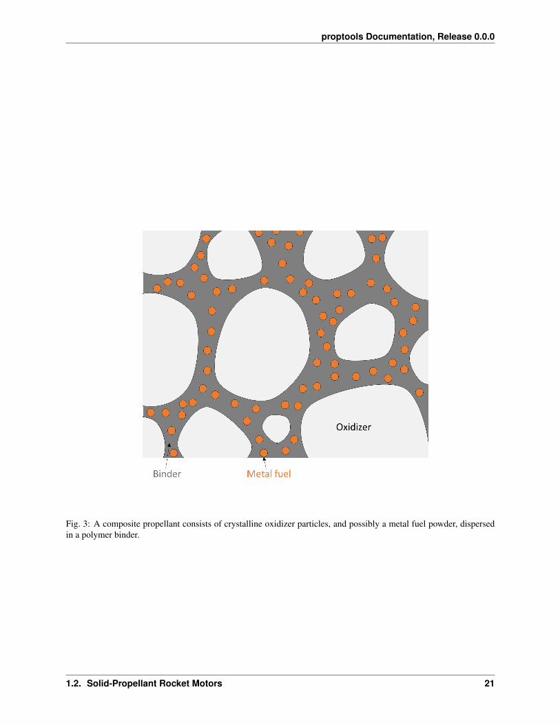
APCP contains a solid oxidizer (ammonium perchlorate) and (optionally) a powdered metal fuel, held together by arubber-like binder. Ammonium perchlorate is a crystalline solid, which divided into small particles (10 to 500 𝜇m)and dispersed though the propellant. During combustion, the ammonium perchlorate decomposes to produce a gasrich in oxidizing species. A polymer matrix, the binder, binds the oxidizer particles together, giving the propellantmechanical strength. The binder serves as a fuel, giving off hydrocarbon vapors during combustion. Additional fuelmay be added as hot-burning metal powder dispersed in the binder.

1.2.3 Combustion Process

The combustion process of a composite propellant has many steps, and the flame structure is complex. Although thepropellant is a solid, important reactions, including combustion of the fuel with the oxidizer, occur in the gas phase.A set of flames hover over the surface of the burning propellant. These flames transfer heat to the propellant surface,causing its solid components to decompose into gases. The gaseous decomposition products contain fuel vapor andoxidizing species, which supply the flames with reactants.

Importantly, the combustion process contains a feedback loop. Heat from the flames vaporizes the surface, and vaporfrom the surface provides fuel and oxidizer to the flames. The rate at which this process proceeds depends on chemicalkinetics, mass transfer, and heat transfer within the combustion zone. Importantly, the feedback rate depends onpressure. As we will see in the next section, the rate of propellant combustion determines the chamber pressure andthrust of a solid rocket motor.

Effect of pressure on burn rate

The flame structure described above causes the propellant to burn faster at higher pressures. At higher pressures, thegas phase is denser, causing reactions and diffusion to proceed more quickly. This moves the flame structure closer tothe surface. The closer flames and denser conducing medium enhance heat transfer to the surface, which drives moredecomposition, increasing the burn rate.



Fig. 3: A composite propellant consists of crystalline oxidizer particles, and possibly a metal fuel powder, dispersedin a polymer binder.



Fig. 4: The typical flame structure of composite propellant combustion. Heat from the flames decomposes the ammo-nium perchlorate and binder, which in turn supply oxidizing (AP) and fuel (binder) gases to the flames.



Although this dependence is complicated, it can be empirically described by Vieille’s Law, which relates the burn rate𝑟 to the chamber pressure 𝑝𝑐 via two parameters:

𝑟 = 𝑎(𝑝𝑐)𝑛

𝑟 is the rate at which the surface regresses, and has units of velocity. 𝑎 is the burn rate coefficient, which has unitsof [velocity (pressure) -n]. 𝑛 is the unitless burn rate exponent. The model parameters 𝑎, 𝑛 must be determined bycombustion experiments on the propellant.

1.2.4 Motor Internal Ballistics

The study of propellant combustion and fluid dynamics within a rocket motor is called internal ballistics. Internalballistics can be used to estimate the chamber pressure and thrust of a motor.

Equilibrium chamber pressure

The operating chamber pressure of a solid motor is set by an equilibrium between exhaust generation from combustionand exhaust discharge through the nozzle. The chamber pressure of a solid rocket motor is related to the mass ofcombustion gas in the chamber by the Ideal Gas Law:

𝑝𝑐 = 𝑚𝑅𝑇𝑐1

𝑉𝑐

where 𝑅 is the specific gas constant of the combustion gases in the chamber, 𝑇𝑐 is their temperature, and 𝑉𝑐 is thechamber volume. Gas mass is added to the chamber by burning propellant, and mass flows out of the chamber throughthe nozzle. The rate of change of the chamber gas mass is:

𝑑𝑚

𝑑𝑡= �̇�𝑐𝑜𝑚𝑏𝑢𝑠𝑡𝑖𝑜𝑛 − �̇�𝑛𝑜𝑧𝑧𝑙𝑒

Ideal nozzle theory relates the mass flow through the nozzle to the chamber pressure and the Characteristic velocity:

�̇�𝑛𝑜𝑧𝑧𝑙𝑒 =𝑝𝑐𝐴𝑡

𝑐*

The rate of gas addition from combustion is:

�̇�𝑐𝑜𝑚𝑏𝑢𝑠𝑡𝑖𝑜𝑛 = 𝐴𝑏𝜌𝑠𝑟(𝑝𝑐)

where :math:’A_b’ is the burn area of the propellant, 𝜌𝑠 is the density of the solid propellant, and 𝑟(𝑝𝑐) is the burn rate(a function of chamber pressure).

At the equilibrium chamber pressure where the inflow and outflow rates are equal:

𝑑𝑚

𝑑𝑡= �̇�𝑐𝑜𝑚𝑏𝑢𝑠𝑡𝑖𝑜𝑛 − �̇�𝑛𝑜𝑧𝑧𝑙𝑒 = 0

𝐴𝑏𝜌𝑠𝑟(𝑝𝑐) =𝑝𝑐𝐴𝑡

𝑐*

𝑝𝑐 =𝐴𝑏

𝐴𝑡𝜌𝑠𝑐

*𝑟(𝑝𝑐)

= 𝐾𝜌𝑠𝑐*𝑟(𝑝𝑐)

where 𝐾 ≡ 𝐴𝑏

𝐴𝑡is ratio of burn area to throat area. If the propellant burn rate is well-modeled by Vieille’s Law, the

equilibrium chamber pressure can be solved for in closed form:

𝑝𝑐 = (𝐾𝜌𝑠𝑐*𝑎)

11−𝑛

Consider an example motor. The motor burns a relatively slow-burning propellant with the following properties:



• Burn rate exponent of 0.5, and a burn rate of 2.54 mm s -1 at 6.9 MPa

• Exhaust ratio of specific heats of 1.26

• Characteristic velocity of 1209 m s -1

• Solid density of 1510 kg m -3

The motor has a burn area of 1.25 m 2, and a throat area of 839 mm 2 (diameter of 33 mm).

Plot the combustion and nozzle mass flow rates versus pressure:

"""Illustrate the chamber pressure equilibrium of a solid rocket motor."""

from matplotlib import pyplot as pltimport numpy as np

p_c = np.linspace(1e6, 10e6) # Chamber pressure [units: pascal].

# Propellant propertiesgamma = 1.26 # Exhaust gas ratio of specific heats [units: dimensionless].rho_solid = 1510. # Solid propellant density [units: kilogram meter**-3].n = 0.5 # Propellant burn rate exponent [units: dimensionless].a = 2.54e-3 * (6.9e6)**(-n) # Burn rate coefficient, such that the propellant# burns at 2.54 mm s**-1 at 6.9 MPa [units: meter second**-1 pascal**-n].c_star = 1209. # Characteristic velocity [units: meter second**-1].

# Motor geometryA_t = 839e-6 # Throat area [units: meter**2].A_b = 1.25 # Burn area [units: meter**2].

# Compute the nozzle mass flow rate at each chamber pressure.# [units: kilogram second**-1].m_dot_nozzle = p_c * A_t / c_star

# Compute the combustion mass addition rate at each chamber pressure.# [units: kilogram second**-1].m_dot_combustion = A_b * rho_solid * a * p_c**n

# Plot the mass ratesplt.plot(p_c * 1e-6, m_dot_nozzle, label='Nozzle')plt.plot(p_c * 1e-6, m_dot_combustion, label='Combustion')plt.xlabel('Chamber pressure [MPa]')plt.ylabel('Mass rate [kg / s]')

# Find where the mass rates are equal (e.g. the equilibrium).i_equil = np.argmin(abs(m_dot_combustion - m_dot_nozzle))m_dot_equil = m_dot_nozzle[i_equil]p_c_equil = p_c[i_equil]

# Plot the equilibrium point.plt.scatter(p_c_equil * 1e-6, m_dot_equil, marker='o', color='black', label=→˓'Equilibrium')plt.axvline(x=p_c_equil * 1e-6, color='grey', linestyle='--')

plt.title('Chamber pressure: stable equilibrium, $n =$ {:.1f}'.format(n))plt.legend()plt.show()

The nozzle and combustion mass flow rates are equal at 6.9 MPa: this is the equilibrium pressure of the motor. This



2 4 6 8 10Chamber pressure [MPa]

1

2

3

4

5

6

7

Mas

s rat

e [k

g / s

]

Chamber pressure: stable equilibrium, n = 0.5NozzleCombustionEquilibrium



equilibrium is stable:

• At lower pressures, the combustion mass addition rate is higher than the nozzle outflow rate, so the mass of gasin the chamber will increase and the pressure will rise to the equilibrium value.

• At higher pressures, the combustion mass addition rate is lower than the nozzle outflow rate, so the mass of gasin the chamber will decrease and the pressure will fall to the equilibrium value.

In general, a stable equilibrium pressure will exist for propellants with 𝑛 < 1 (i.e. burn rate is sub-linear in pressure).

We can use proptools to quickly find the chamber pressure and thrust of the example motor:

"""Find the chamber pressure and thrust of a solid rocket motor."""from proptools import solid, nozzle


# Motor geometryA_t = 839e-6 # Throat area [units: meter**2].A_b = 1.25 # Burn area [units: meter**2].

# Nozzle exit pressure [units: pascal].p_e = 101e3

# Compute the chamber pressure [units: pascal].p_c = solid.chamber_pressure(A_b / A_t, a, n, rho_solid, c_star)

# Compute the sea level thrust [units: newton].F = nozzle.thrust(A_t, p_c, p_e, gamma)

print 'Chamber pressure = {:.1f} MPa'.format(p_c * 1e-6)print 'Thrust (sea level) = {:.1f} kN'.format(F * 1e-3)

Chamber pressure = 6.9 MPa

Thrust (sea level) = 9.1 kN

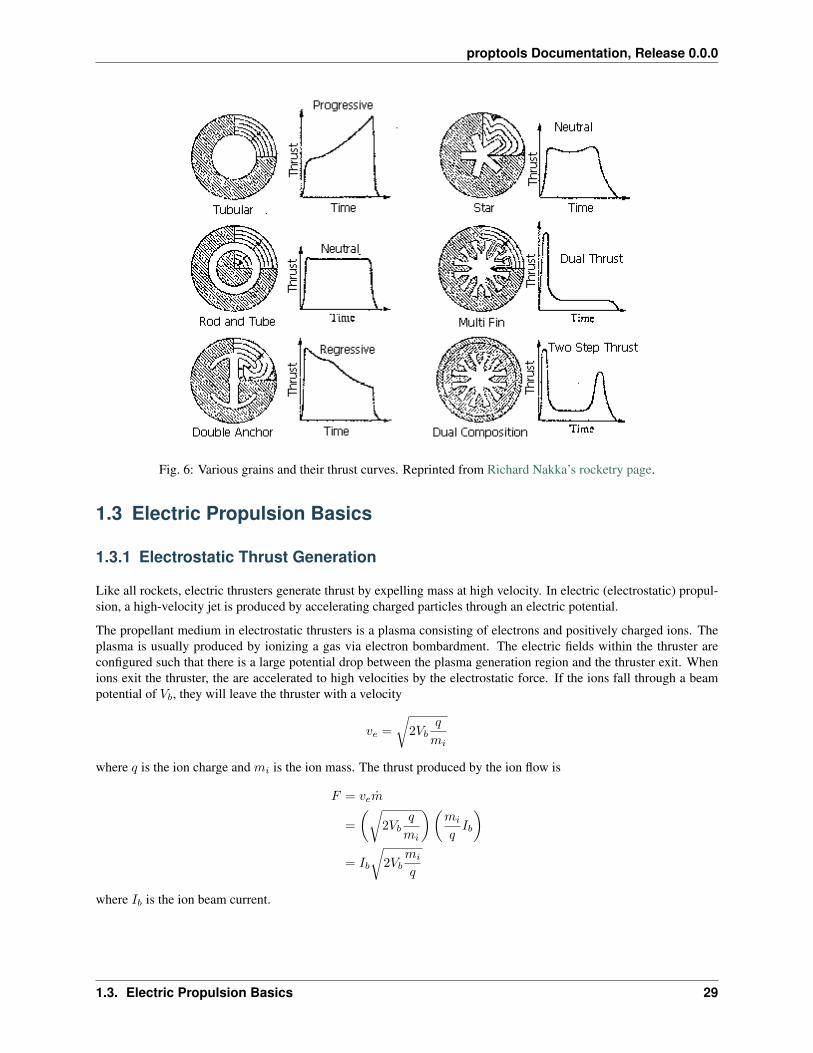
Burn area evolution and thrust curves

In most propellant grain geometries, the burn area of the propellant grain changes as the flame front advances andpropellant is consumed. This change in burn area causes the chamber pressure and thrust to change during the burn.The variation of thrust (or chamber pressure) with time is called a thrust curve. Thrust curves are classified as regressive(decreasing with time), neutral or progressive (increasing with time).

If we know how the burn area 𝐴𝑏 varies with the flame front progress distance 𝑥, we can use proptools to predictthe thrust curve. For example, consider a cylindrical propellant with a hollow circular core. The core radius 𝑟𝑖𝑛 is 0.15m, the outer radius 𝑟𝑜𝑢𝑡 is 0.20 m, and the length 𝐿 is 1.0 m. The burn area is given by:

𝐴𝑏(𝑥) = 2𝜋(𝑟𝑖𝑛 + 𝑥)𝐿



Fig. 5: Dimensions of the example cylindrical propellant grain.

Assume that the propellant properties are the same as in the previous example. The nozzle throat area is still 839 mm2, and the nozzle expansion area ratio is 8.

"""Plot the thrust curve of a solid rocket motor with a cylindrical propellant grain."→˓""

from matplotlib import pyplot as pltimport numpy as npfrom proptools import solid

# Grain geometry (Clinder with circular port)r_in = 0.15 # Grain inner radius [units: meter].r_out = 0.20 # Grain outer radius [units: meter].length = 1.0 # Grain length [units: meter].


# Nozzle geometryA_t = 839e-6 # Throat area [units: meter**2].A_e = 8 * A_t # Exit area [units: meter**2].p_a = 101e3 # Ambeint pressure during motor firing [units: pascal].

# Burning surface evolutionx = np.linspace(0, r_out - r_in) # Flame front progress steps [units: meter].A_b = 2 * np.pi * (r_in + x) * length # Burn area at each flame progress step→˓[units: meter**2].

# Compute thrust curve.t, p_c, F = solid.thrust_curve(A_b, x, A_t, A_e, p_a, a, n, rho_solid, c_star, gamma)

# Plot results.ax1 = plt.subplot(2, 1, 1)





plt.plot(t, p_c * 1e-6)plt.ylabel('Chamber pressure [MPa]')

ax2 = plt.subplot(2, 1, 2)plt.plot(t, F * 1e-3)plt.ylabel('Thrust, sea level [kN]')plt.xlabel('Time [s]')plt.setp(ax1.get_xticklabels(), visible=False)

plt.tight_layout()plt.subplots_adjust(hspace=0)plt.show()

4.0

4.5

5.0

5.5

6.0

6.5

7.0

Cham

ber p

ress

ure

[MPa

]

0 5 10 15 20Time [s]

5

6

7

8

9

Thru

st, s

ea le

vel [

kN]

Note that the pressure and thrust increase with time (the thrust curve is progressive). This grain has a progressivethrust curve because the burn area increases with 𝑥 as the flame front moves outward from the initial core.

Solid motor designers have devised a wide variety of grain geometries to achieve different thrust curves.



Fig. 6: Various grains and their thrust curves. Reprinted from Richard Nakka’s rocketry page.

1.3 Electric Propulsion Basics

1.3.1 Electrostatic Thrust Generation

Like all rockets, electric thrusters generate thrust by expelling mass at high velocity. In electric (electrostatic) propul-sion, a high-velocity jet is produced by accelerating charged particles through an electric potential.

The propellant medium in electrostatic thrusters is a plasma consisting of electrons and positively charged ions. Theplasma is usually produced by ionizing a gas via electron bombardment. The electric fields within the thruster areconfigured such that there is a large potential drop between the plasma generation region and the thruster exit. Whenions exit the thruster, the are accelerated to high velocities by the electrostatic force. If the ions fall through a beampotential of 𝑉𝑏, they will leave the thruster with a velocity

𝑣𝑒 =

√︂2𝑉𝑏

𝑞

𝑚𝑖

where 𝑞 is the ion charge and 𝑚𝑖 is the ion mass. The thrust produced by the ion flow is

𝐹 = 𝑣𝑒�̇�

=

(︂√︂2𝑉𝑏

𝑞

𝑚𝑖

)︂(︂𝑚𝑖

𝑞𝐼𝑏

)︂= 𝐼𝑏

√︂2𝑉𝑏

𝑚𝑖

𝑞

where 𝐼𝑏 is the ion beam current.

1.3. Electric Propulsion Basics 29

https://www.nakka-rocketry.net


The ideal specific impulse of an electrostatic thruster is:

𝐼𝑠𝑝 =𝑣𝑒𝑔0

=1

𝑔0

√︂2𝑉𝑏

𝑞

𝑚𝑖

As an example, use proptools to compute the thrust and specific impulse of singly charged Xenon ions with abeam voltage of 1000 V and a beam current of 1 A:

"""Example electric propulsion thrust and specific impulse calculation."""from proptools import electric, constants

V_b = 1000. # Beam voltage [units: volt].I_b = 1. # Beam current [units: ampere].F = electric.thrust(I_b, V_b, electric.m_Xe)I_sp = electric.specific_impulse(V_b, electric.m_Xe)m_dot = F / (I_sp * constants.g)print 'Thrust = {:.1f} mN'.format(F * 1e3)print 'Specific Impulse = {:.0f} s'.format(I_sp)print 'Mass flow = {:.2f} mg s^-1'.format(m_dot * 1e6)

Thrust = 52.2 mN

Specific Impulse = 3336 s

Mass flow = 1.59 mg s^-1

This example illustrates the typical performance of electric propulsion systems: low thrust, high specific impulse, andlow mass flow.

1.3.2 Advantages over Chemical Propulsion

Electric propulsion is appealing because it enables higher specific impulse than chemical propulsion. The specificimpulse of a chemical rocket depends on velocity to which a nozzle flow can be accelerated. This velocity is limitedby the finite energy content of the working gas. In contrast, the particles leaving an electric thruster can be acceleratedto very high velocities if sufficient electrical power is available.

In a chemical rocket, the kinetic energy of the exhaust gas is supplied by thermal energy released in a combustionreaction. For example, in the stoichiometric combustion of H2 and O2 releases an energy per particle of 4.01 × 10−19

J, or 2.5 eV. If all of the released energy were converted into kinetic energy of the exhaust jet, the maximum possibleexhaust velocity would be:

𝑣𝑒 =

√︃2

𝐸

𝑚𝐻2𝑂= 5175 ms−1

corresponding to a maximum specific impulse of about 530 s. In practice, the most efficient flight engines have specificimpulses of 450 to 500 s.

With electric propulsion, much higher energies per particle are possible. If we accelerate (singly) charged particlesthrough a potential of 1000 V, the jet kinetic energy will be 1000 eV per ion. This is 400 times more energy per particlethan is possible with chemical propulsion (or, for similar particle masses, 20 times higher specific impulse). Specificimpulse in excess of 10,000 s is feasible with electric propulsion.



1.3.3 Power and Efficiency

In an electric thruster, the energy to accelerate the particles in the jet must be supplied by an external source. Typicallysolar panels supply this electrical power, but some future concepts might use nuclear reactors. The available powerlimits the thrust and specific impulse of an electric thruster.

The kinetic power of the jet is given by:

𝑃𝑗𝑒𝑡 =𝐹 2

2�̇�

where �̇� is the jet mass flow. Increasing thrust with increasing mass flow (i.e. increasing 𝐼𝑠𝑝) will increase the kineticpower of the jet.

The power input required by the thruster (𝑃𝑖𝑛) is somewhat higher than the jet power. The ratio of the jet and inputpower is the total efficiency of the thruster, 𝜂𝑇 :

𝜂𝑇 ≡ 𝑃𝑗𝑒𝑡

𝑃𝑖𝑛

The total efficiency depends on several factors:

1. Thrust losses due to beam divergence. This loss is proportional to the cosine of the average beam divergencehalf-angle.

2. Thrust losses due to doubly charged ions in the beam. This loss is a function of the doubles-to-singles currentratio, 𝐼++/𝐼+

3. Thrust losses due to propellant gas escaping the thruster without being ionized. The fraction of the propellantmass flow which is ionized and enters the beam is the mass utilization efficiency, 𝜂𝑚.

4. Electrical losses incurred in ion generation, power conversion, and powering auxiliary thruster components.These losses are captured by the electrical efficiency, 𝜂𝑒 = 𝐼𝑏𝑉𝑏

𝑃𝑖𝑛

Use proptools to compute the efficiency and required power of the example thruster. Assume that the beamdivergence is cos(10𝑥𝑏0), the double ion current fraction is 10%, the mass utilization efficiency is 90%, and theelectrical efficiency is 85%:

"""Example electric propulsion power calculation."""import numpy as npfrom proptools import electric

F = 52.2e-3 # Thrust [units: newton].m_dot = 1.59e-6 # Mass flow [units: kilogram second**-1].

# Compute the jet power [units: watt].P_jet = electric.jet_power(F, m_dot)

# Compute the total efficiency [units: dimensionless].eta_T = electric.total_efficiency(

divergence_correction=np.cos(np.deg2rad(10)),double_fraction=0.1,mass_utilization=0.9,electrical_efficiency=0.85)

# Compute the input power [units: watt].P_in = P_jet / eta_T

print 'Jet power = {:.0f} W'.format(P_jet)print 'Total efficiency = {:.3f}'.format(eta_T)print 'Input power = {:.0f} W'.format(P_in)



Jet power = 857 W

Total efficiency = 0.703

Input power = 1219 W

The overall efficiency of the thruster is about 70%. The required input power could be supplied by a few square metersof solar panels (at 1 AU from the sun).

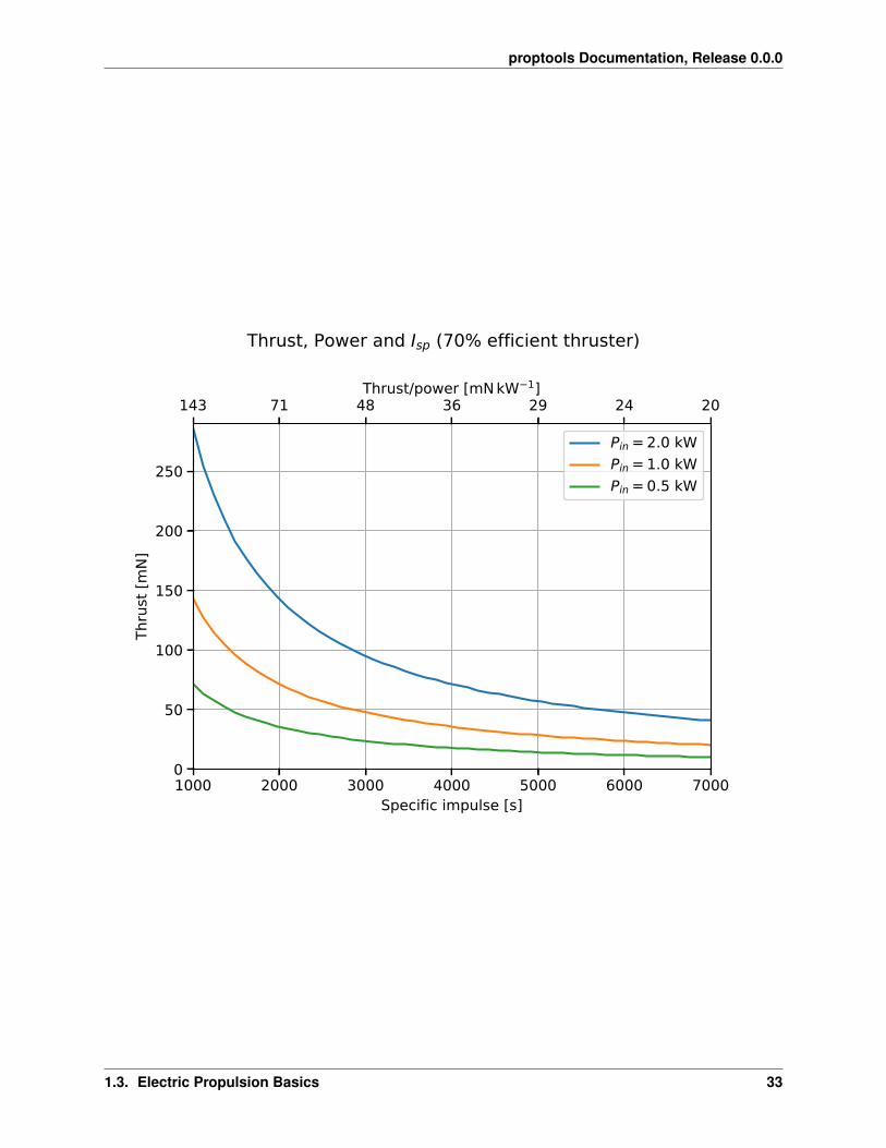
The power, thrust, and specific impulse of a thruster are related by:

𝐹

𝑃𝑖𝑛=

2𝜂𝑇𝑔0𝐼𝑠𝑝

Thus, for a power-constrained system the propulsion designer faces a trade-off between thrust and specific impulse.

"""Plot the thrust, power, Isp trade-off."""from matplotlib import pyplot as pltimport numpy as npfrom proptools import electric

eta_T = 0.7 # Total efficiency [units: dimensionless].I_sp = np.linspace(1e3, 7e3) # Specific impulse [units: second].

ax1 = plt.subplot(111)for P_in in [2e3, 1e3, 500]:

T = P_in * electric.thrust_per_power(I_sp, eta_T)plt.plot(I_sp, T * 1e3, label='$P_{{in}} = {:.1f}$ kW'.format(P_in * 1e-3))

plt.xlim([1e3, 7e3])plt.ylim([0, 290])plt.xlabel('Specific impulse [s]')plt.ylabel('Thrust [mN]')plt.legend()plt.suptitle('Thrust, Power and $I_{sp}$ (70% efficient thruster)')plt.grid(True)

# Add thrust/power on second axis.ax2 = ax1.twiny()new_tick_locations = ax1.get_xticks()ax2.set_xlim(ax1.get_xlim())ax2.set_xticks(new_tick_locations)ax2.set_xticklabels(['{:.0f}'.format(tp * 1e6)

for tp in electric.thrust_per_power(new_tick_locations, eta_T)])ax2.set_xlabel('Thrust/power [$\\mathrm{mN \\, kW^{-1}}$]')ax2.tick_params(axis='y', direction='in', pad=-25)plt.subplots_adjust(top=0.8)

plt.show()

1.3.4 Optimal Specific Impulse

For electrically propelled spacecraft, there is an optimal specific impulse which will maximize the payload massfraction of a given mission. While increasing specific impulse decreases the required propellant mass, it also increasesthe required power at a particular thrust level, which increases the mass of the power supply. The optimal specificimpulse minimizes the combined mass of the propellant and power supply.



1000 2000 3000 4000 5000 6000 7000Specific impulse [s]

0

50

100

150

200

250

Thru

st [m

N]

Pin = 2.0 kWPin = 1.0 kWPin = 0.5 kW

143 71 48 36 29 24 20Thrust/power [mN kW 1]

Thrust, Power and Isp (70% efficient thruster)



The optimal specific impulse depends on several factors:

1. The mission thrust duration, 𝑡𝑚. Longer thrust durations reduce the required thrust (if the same total impulse or∆𝑣 is to be delivered), and therefore reduce the power and power supply mass at a given 𝐼𝑠𝑝. Therefore, longerthrust durations increase the optimal 𝐼𝑠𝑝.

2. The specific mass of the power supply, 𝛼. This is the ratio of power supply mass to power, and is typically 20 to200 kg kW -1 for solar-electric systems. The specific impulse optimization assumes that power supply mass islinear with respect to power. Increasing the specific mass reduces the optimal 𝐼𝑠𝑝.

3. The total efficiency of the thruster.

4. The ∆𝑣 of the mission. Higher ∆𝑣 (in a fixed time window) requires more thrust, and therefore leads to a loweroptimal 𝐼𝑠𝑝.

Consider an example mission to circularize the orbit of a geostationary satellite launched onto a elliptical transferorbit. Assume that the low-thrust circularization maneuver requires a ∆𝑣 of 2 km s -1 over 100 days. The thruster is70% efficient and the power supply specific mass is 50 kg kW -1:

"""Example calculation of optimal specific impulse for an electrically propelled→˓spacecraft."""from proptools import electric

dv = 2e3 # Delta-v [units: meter second**-1].t_m = 100 * 24 * 60 * 60 # Thrust duration [units: second].eta_T = 0.7 # Total efficiency [units: dimensionless].specific_mass = 50e-3 # Specific mass of poower supply [units: kilogram watt**-1].I_sp = electric.optimal_isp_delta_v(dv, eta_T, t_m, specific_mass)

print 'Optimal specific impulse = {:.0f} s'.format(I_sp)

Optimal specific impulse = 1482 s

For the mathematical details of specific impulse optimization, see [Lozano].


CHAPTER 2

Package contents

2.1 proptools

2.1.1 proptools package

Submodules

proptools.constants module

Physical Constants.

Matt Vernacchia proptools 2016 Apr 15

proptools.isentropic module

Isentropic relations.

See Isentropic Relations for a physical explaination of the isentropic relations.

stag_temperature_ratio(M, gamma) Stagnation temperature / static temperature ratio.stag_pressure_ratio(M, gamma) Stagnation pressure / static pressure ratio.stag_density_ratio(M, gamma) Stagnation density / static density ratio.velocity(v_1, p_1, T_1, p_2, gamma, m_molar) Velocity relation between two points in an isentropic

flow.

proptools.isentropic.stag_density_ratio(M, gamma)Stagnation density / static density ratio.

Parameters

• M (scalar) – Mach number [units: dimensionless].

35


• gamma (scalar) – Heat capacity ratio [units: dimensionless].

Returns the stagnation density ratio 𝜌0/𝜌 [units: dimensionless].

Return type scalar

proptools.isentropic.stag_pressure_ratio(M, gamma)Stagnation pressure / static pressure ratio.

Parameters



Returns the stagnation pressure ratio 𝑝0/𝑝 [units: dimensionless].

Return type scalar

proptools.isentropic.stag_temperature_ratio(M, gamma)Stagnation temperature / static temperature ratio.

Parameters



Returns the stagnation temperature ratio 𝑇0/𝑇 [units: dimensionless].

Return type scalar

proptools.isentropic.velocity(v_1, p_1, T_1, p_2, gamma, m_molar)Velocity relation between two points in an isentropic flow.

Given the velocity, pressure, and temperature at station 1 and the pressure at station 2, find the velocity at station2. See Rocket Propulsion Elements, 8th edition, equation 3-15b.

Parameters

• v_1 (scalar) – Velocity at station 1 [units: meter second**-1].

• p_1 (scalar) – Pressure at station 1 [units: pascal].

• T_1 (scalar) – Temperature at station 1 [units kelvin].

• p_2 (scalar) – Pressure at station 2 [units: pascal].

• gamma (scalar) – Gas ratio of specific heats [units: dimensionless].

• m_molar (scalar) – Gas mean molar mass [units: kilogram mole**-1].

Returns velocity at station 2 [units: meter second**-1].

Return type scalar

proptools.electric package

Electric propulsion design tools.

m_Xe float(x) -> floating point numberm_Kr float(x) -> floating point numberthrust(I_b, V_b, m_ion) Thrust of an electric thruster.jet_power(F, m_dot) Jet power of a rocket propulsion device.

Continued on next page

36 Chapter 2. Package contents


Table 2 – continued from previous pagedouble_ion_thrust_correction(double_fraction)Doubly-charged ion thrust correction factor.specific_impulse(V_b, m_ion[, . . . ]) Specific impulse of an electric thruster.total_efficiency([divergence_correction, . . . ]) Total efficiency of an electric thruster.thrust_per_power(I_sp[, total_efficiency]) Thrust/power ratio of an electric thruster.stuhlinger_velocity(total_efficiency, t_m, . . . ) Stuhlinger velocity, a characteristic velocity for electric

propulsion missions.optimal_isp_thrust_time(total_efficiency,. . . )

Optimal specific impulse for constant thrust / fixed timemission.

optimal_isp_delta_v(dv, total_efficiency, . . . ) Optimal specific impulse for a fixed ∆𝑣 mission.

proptools.electric.double_ion_thrust_correction(double_fraction)Doubly-charged ion thrust correction factor.

Compute the thrust correction factor for the presence of doubly charged ions in the beam. This factor is denotedas 𝛼 in Goebel and Katz.

Reference: Goebel and Katz, equation 2.3-14.

Parameters double_fraction (scalar in [0, 1]) – The doubly-charged ion currentover the singly-charged ion current, 𝐼++/𝐼+ [units: dimensionless].

Returns The thrust correction factor, 𝛼 [units: dimensionless].

Return type scalar in (0, 1]

proptools.electric.jet_power(F, m_dot)Jet power of a rocket propulsion device.

Compute the kinetic power of the jet for a given thrust level and mass flow.


Parameters

• F (scalar) – Thrust force [units: newton].

• m_dot (scalar) – Jet mass flow rate [units: kilogram second**-1].

Returns jet power [units: watt].

Return type scalar

proptools.electric.optimal_isp_delta_v(dv, total_efficiency, t_m, specific_mass, dis-charge_loss=None, m_ion=None)

Optimal specific impulse for a fixed ∆𝑣 mission.

The dependence of efficiency on specific impulse can optionally be included in the optimization. Ifdischarge_loss and m_ion are not provided, then the total efficiency 𝜂𝑇 has a constant value of thegiven total_efficiency. If discharge_loss and m_ion are provided, 𝜂𝑇 is assumed to vary withspecific impulse as:

𝜂𝑇 =𝜂𝑇,0

1+(𝑣𝐿/𝐼𝑠𝑝𝑔)2

where 𝜂𝑇,0 is the given value of total_efficiency, and 𝑣𝐿 is the loss velocity:

𝑣𝐿 =√︀

2𝑞𝑉𝑑/𝑚𝑖

where 𝑉𝑑 is the discharge loss and 𝑚𝑖 is the ion mass.

Reference: Lozano 16.522 notes, equation 3-13.

Parameters

2.1. proptools 37

https://ocw.mit.edu/courses/aeronautics-and-astronautics/16-522-space-propulsion-spring-2015/lecture-notes/MIT16_522S15_Lecture3-4.pdf


• total_efficiency (scalar in (0, 1]) – The total efficiency of the thruster[units: dimensionless].

• t_m – mission thrust duration [units: second].

• specific_mass – specific mass (per unit power) of the thruster and power system [units:kilogram watt**1].

• discharge_loss (scalar, optional) – The discharge loss per ion [units: volt].

• m_ion (scalar, optional) – Ion mass [units: kilogram].

Returns Optimal specific impulse [units: second].

Return type scalar

proptools.electric.optimal_isp_thrust_time(total_efficiency, t_m, specific_mass)Optimal specific impulse for constant thrust / fixed time mission.


Parameters



• specific_mass (scalar) – specific mass (per unit power) of the thruster and powersystem [units: kilogram watt**1].

Returns Optimal specific impulse [units: second].

Return type scalar

proptools.electric.specific_impulse(V_b, m_ion, divergence_correction=1, dou-ble_fraction=1, mass_utilization=1)

Specific impulse of an electric thruster.

If only V_b and m_ion are provided, the ideal specific impulse will be computed. Ifdivergence_correction, double_fraction, or mass_utilization are provided, the specificimpulse will be reduced by the corresponding efficiency factors.


Parameters

• V_b (scalar) – Beam voltage [units: volt].

• m_ion (scalar) – Ion mass [units: kilogram].

• divergence_correction (scalar in (0, 1])) – Thrust correction factor forbeam divergence [units: dimensionless].

• double_fraction (scalar in [0, 1]) – The doubly-charged ion current over thesingly-charged ion current, 𝐼++/𝐼+ [units: dimensionless].

• mass_utilization (scalar in (0, 1])) – Mass utilization efficiency [units: di-mensionless].

Returns the specific impulse [units: second].

Return type scalar

proptools.electric.stuhlinger_velocity(total_efficiency, t_m, specific_mass)Stuhlinger velocity, a characteristic velocity for electric propulsion missions.




The Stuhlinger velocity is a characteristic velocity for electric propulsion missions, and is used in calculation ofoptimal specific impulse. It is defined as:

𝑣𝑐ℎ ≡√︁

2𝜂𝑇 𝑡𝑚𝛼

where 𝜂𝑇 is the thruster total efficiency, 𝑡𝑚 is the mission thrust duration, and 𝛼 is the propulsion and powersystem specific mass.

The Stuhlinger velocity is also an approximate upper limit for the ∆𝑣 capability of an electric propulsion space-craft.


Parameters



• specific_mass – specific mass (per unit power) of the thruster and power system [units:kilogram watt**1].

Returns Stuhlinger velocity [units: meter second**-1].

Return type scalar

proptools.electric.thrust(I_b, V_b, m_ion)Thrust of an electric thruster.

Compute the ideal thrust of an electric thruster from the beam current and voltage, assuming singly charged ionsand no beam divergence.


Parameters

• I_b (scalar) – Beam current [units: ampere].

• V_b (scalar) – Beam voltage [units: volt].

• m_ion (scalar) – Ion mass [units: kilogram].

Returns Thrust force [units: newton].

Return type scalar

proptools.electric.thrust_per_power(I_sp, total_efficiency=1)Thrust/power ratio of an electric thruster.


Parameters

• I_sp (scalar) – Specific impulse [units:second].


Returns Thrust force per unit power input [units: newton watt**-1].

Return type scalar

proptools.electric.total_efficiency(divergence_correction=1, double_fraction=1,mass_utilization=1, electrical_efficiency=1)

Total efficiency of an electric thruster.

The total efficiency is defined as the ratio of jet power to input power:

2.1. proptools 39



𝜂𝑇 ≡ 𝑃𝑗𝑒𝑡

𝑃𝑖𝑛


Parameters

• divergence_correction (scalar in (0, 1])) – Thrust correction factor forbeam divergence [units: dimensionless].

• double_fraction (scalar in [0, 1]) – The doubly-charged ion current over thesingly-charged ion current, 𝐼++/𝐼+ [units: dimensionless].

• mass_utilization (scalar in (0, 1])) – Mass utilization efficiency [units: di-mensionless].

• electrical_efficiency (scalar in (0, 1])) – Electrical efficiency [units:dimensionless].

Returns Total efficiency [units: dimensionless].

Return type scalar

proptools.isentropic_test module

Unit test for isentropic relations.

class proptools.isentropic_test.TestStagDesnityRatio(methodName=’runTest’)Bases: unittest.case.TestCase

Unit tests for isentropic.stag_density_ratio

test_sonic()Check the ratio when Mach=1.

test_still()Check that the ratio is 1 when Mach=0.

class proptools.isentropic_test.TestStagPressureRatio(methodName=’runTest’)Bases: unittest.case.TestCase

Unit tests for isentropic.stag_pressure_ratio



class proptools.isentropic_test.TestStagTemperatureRatio(methodName=’runTest’)Bases: unittest.case.TestCase

Unit tests for isentropic.stag_temperature_ratio



class proptools.isentropic_test.TestVelocity(methodName=’runTest’)Bases: unittest.case.TestCase

Unit tests for isentropic.velocity.



test_equal_pressure()Test that the velocity is the same if the pressure is the same.

test_rpe_3_2()Test against example problem 3-2 from Rocket Propulsion Elements.

proptools.nonsimple_comp_flow module

Non-simple compressible flow.

Calculate quasi-1D compressible flow properties with varying area, friction, and heat addition. “One-dimensionalcompressible flows of calorically perfect gases in which only a single driving potential is present are called simpleflows” [1]. This module implements a numerical solution for non-simple flows, i.e. flows with multiple drivingpotentials.

References

[1] L. Pekker, “One-Dimensional Compressible Flow in Variable Area Duct with Heat Addition,” AirForce Research Laboratory, Edwards, CA, Rep. AFRL-RZ-ED-JA-2010-303, 2010. Online:http://www.dtic.mil/dtic/tr/fulltext/u2/a524450.pdf.

[2] A. Bandyopadhyay and A. Majumdar, “Modeling of Compressible Flow with Friction and Heat Transferusing the Generalized Fluid System Simulation Program (GFSSP),” Thermal Fluid Analysis Workshop,Cleveland, OH, 2007. Online: https://tfaws.nasa.gov/TFAWS07/Proceedings/TFAWS07-1016.pdf

[3] J. D. Anderson, Modern Compressible Flow with Historical Perspective, 2nd ed. New York, NY: McGraw-Hill, 1990.

Matt Vernacchia proptools 2016 Oct 3

proptools.nonsimple_comp_flow.differential(x, state, mdot, c_p, gamma, f_f, f_q, f_A)Differential equation for Mach number in non-simple duct flow.

Note: This method will not be accurate (and may divide by zero) for flows which contain a region at Mach 1,e.g. a choked convergent-divergent nozzle.

Parameters

• state (2-vector) – Stagnation temperature [units: kelvin], Mach number [units: none].

• x (scalar) – Distance from the duct inlet [units: meter].

• mdot (scalar) – The mass flow through the duct [units: kilogram second**-1].

• c_p (scalar) – Fluid heat capacity at constant pressure [units: joule kilogram**-1kelvin**-1].

• gamma (scalar) – Fluid ratio of specific heats [units: none].

• f_f (function mapping scalar->scalar) – The Fanning friction factor as afunction of distance from the inlet [units: none].

• f_q (function mapping scalar->scalar) – The heat transfer into the fluid perunit wall area as a function of distance from the inlet [units: joule meter**-2].

• f_A (function mapping scalar->scalar) – The duct area as a function of dis-tance from the inlet [units: meter**2].

Returns d state / dx

proptools.nonsimple_comp_flow.main()

2.1. proptools 41

http://www.dtic.mil/dtic/tr/fulltext/u2/a524450.pdf

https://tfaws.nasa.gov/TFAWS07/Proceedings/TFAWS07-1016.pdf


proptools.nonsimple_comp_flow.solve_nonsimple(x, M_in, T_o_in, mdot, c_p, gamma, f_f,f_q, f_A)

Solve a non-simple flow case

Parameters

• state (2-vector) – Stagnation temperature [units: kelvin], Mach number [units: none].

• x (array) – Distances from the duct inlet at which to return solution [units: meter].

• T_o_in (scalar) – Inlet stagnation temperature [units: kelvin].

• M_in (scalar) – Inlet Mach number [units: none].

• mdot (scalar) – The mass flow through the duct [units: kilogram second**-1].

• c_p (scalar) – Fluid heat capacity at constant pressure [units: joule kilogram**-1kelvin**-1].

• gamma (scalar) – Fluid ratio of specific heats [units: none].

• f_f (function mapping scalar->scalar) – The Fanning friction factor as afunction of distance from the inlet [units: none].

• f_q (function mapping scalar->scalar) – The heat transfer into the fluid perunit wall area as a function of distance from the inlet [units: joule meter**-2].

• f_A (function mapping scalar->scalar) – The duct area as a function of dis-tance from the inlet [units: meter**2].

Returns

The stagnation temperature at each station in x [units: none]. M (array of length len(x)): TheMach number at each station in x [units: none]. choked (boolean): True if the flow chokes atM=1 in the duct. M and T_o for x past the

choke point will be nan. Choking can cause shocks or upstream effects which this modeldoes not capture; therefore results for choked scenarios may not be accurate.

Return type T_o (array of length len(x))

proptools.nozzle module

Nozzle flow calculations.

thrust_coef(p_c, p_e, gamma[, p_a, er]) Nozzle thrust coefficient, 𝐶𝐹 .c_star(gamma, m_molar, T_c) Characteristic velocity, 𝑐*.er_from_p(p_c, p_e, gamma) Find the nozzle expansion ratio from the chamber and

exit pressures.throat_area(m_dot, p_c, T_c, gamma, m_molar) Find the nozzle throat area.mass_flow(A_t, p_c, T_c, gamma, m_molar) Find the mass flow through a choked nozzle.thrust(A_t, p_c, p_e, gamma[, p_a, er]) Nozzle thrust force.mach_from_er(er, gamma) Find the exit Mach number from the area expansion ra-

tio.mach_from_pr(p_c, p_e, gamma) Find the exit Mach number from the pressure ratio.is_choked(p_c, p_e, gamma) Determine whether the nozzle flow is choked.mach_from_area_subsonic(area_ratio, gamma) Find the Mach number as a function of area ratio for

subsonic flow.area_from_mach(M, gamma) Find the area ratio for a given Mach number.

Continued on next page



Table 3 – continued from previous pagepressure_from_er(er, gamma) Find the exit/chamber pressure ratio from the nozzle ex-

pansion ratio.

proptools.nozzle.area_from_mach(M, gamma)Find the area ratio for a given Mach number.

For isentropic nozzle flow, a station where the Mach number is 𝑀 will have an area 𝐴. This function returnsthat area, normalized by the area of the nozzle throat 𝐴𝑡. See Mach-Area Relation for a physical description ofthe Mach-Area relation.

Reference: Rocket Propulsion Elements, 8th Edition, Equation 3-14.

Parameters


• gamma (scalar) – Ratio of specific heats [units: dimensionless].

Returns Area ratio 𝐴/𝐴𝑡.

Return type scalar

proptools.nozzle.c_star(gamma, m_molar, T_c)Characteristic velocity, 𝑐*.

The characteristic velocity is a figure of merit for the propellants and combustion process. See Characteristicvelocity for a description of the physical meaning of the characteristic velocity.

Reference: Equation 1-32a in Huzel and Huang.

Parameters

• gamma (scalar) – Exhaust gas ratio of specific heats [units: dimensionless].

• m_molar (scalar) – Exhaust gas mean molar mass [units: kilogram mole**-1].

• T_c (scalar) – Nozzle stagnation temperature [units: kelvin].

Returns The characteristic velocity [units: meter second**-1].

Return type scalar

proptools.nozzle.er_from_p(p_c, p_e, gamma)Find the nozzle expansion ratio from the chamber and exit pressures.

See Expansion Ratio for a physical description of the expansion ratio.

Reference: Rocket Propulsion Elements, 8th Edition, Equation 3-25

Parameters

• p_c (scalar) – Nozzle stagnation chamber pressure [units: pascal].

• p_e (scalar) – Nozzle exit static pressure [units: pascal].


Returns Expansion ratio 𝜖 = 𝐴𝑒/𝐴𝑡 [units: dimensionless]

Return type scalar

proptools.nozzle.is_choked(p_c, p_e, gamma)Determine whether the nozzle flow is choked.

See Choked Flow for details.


2.1. proptools 43


Parameters




Returns True if flow is choked, false otherwise.

Return type bool

proptools.nozzle.mach_from_area_subsonic(area_ratio, gamma)Find the Mach number as a function of area ratio for subsonic flow.

Parameters

• area_ratio (scalar) – Area / throat area [units: dimensionless].

• gamma (scalar) – Ratio of specific heats [units: dimensionless].

Returns Mach number of the flow in a passage with area = area_ratio * (throatarea).

Return type scalar

proptools.nozzle.mach_from_er(er, gamma)Find the exit Mach number from the area expansion ratio.

Reference: J. Majdalani and B. A. Maickie, http://maji.utsi.edu/publications/pdf/HT02_11.pdf

Parameters

• er (scalar) – Nozzle area expansion ratio, A_e / A_t [units: dimensionless].


Returns The exit Mach number [units: dimensionless].

Return type scalar

proptools.nozzle.mach_from_pr(p_c, p_e, gamma)Find the exit Mach number from the pressure ratio.

Parameters




Returns Exit Mach number [units: dimensionless].

Return type scalar

proptools.nozzle.mass_flow(A_t, p_c, T_c, gamma, m_molar)Find the mass flow through a choked nozzle.

Given gas stagnation conditions and a throat area, find the mass flow through a choked nozzle. See Choked Flowfor details.


Parameters

• A_t (scalar) – Nozzle throat area [units: meter**2].



http://maji.utsi.edu/publications/pdf/HT02_11.pdf





Returns Mass flow rate �̇� [units: kilogram second**-1].

Return type scalar

proptools.nozzle.pressure_from_er(er, gamma)Find the exit/chamber pressure ratio from the nozzle expansion ratio.

See Expansion Ratio for a physical description of the expansion ratio.


Parameters

• er (scalar) – Expansion ratio 𝜖 = 𝐴𝑒/𝐴𝑡 [units: dimensionless].


Returns Pressure ratio 𝑝𝑒/𝑝𝑐 [units: dimensionless].

Return type scalar

proptools.nozzle.throat_area(m_dot, p_c, T_c, gamma, m_molar)Find the nozzle throat area.

Given gas stagnation conditions and a mass flow rate, find the required throat area of a choked nozzle. SeeChoked Flow for details.


Parameters

• m_dot (scalar) – Propellant mass flow rate [units: kilogram second**-1].





Returns Throat area [units: meter**2].

Return type scalar

proptools.nozzle.thrust(A_t, p_c, p_e, gamma, p_a=None, er=None)Nozzle thrust force.

Parameters





• p_a (scalar, optional) – Ambient pressure [units: pascal]. If None, then p_a = p_e.

• er (scalar, optional) – Nozzle area expansion ratio [units: dimensionless]. If None,then p_a = p_e.

Returns Thrust force [units: newton].

2.1. proptools 45


Return type scalar

proptools.nozzle.thrust_coef(p_c, p_e, gamma, p_a=None, er=None)Nozzle thrust coefficient, 𝐶𝐹 .

The thrust coefficient is a figure of merit for the nozzle expansion process. See Thrust coefficient for a descriptionof the physical meaning of the thrust coefficient.

Reference: Equation 1-33a in Huzel and Huang.

Parameters




• p_a (scalar, optional) – Ambient pressure [units: pascal]. If None, then p_a = p_e.

• er (scalar, optional) – Nozzle area expansion ratio [units: dimensionless]. If None,then p_a = p_e.

Returns The thrust coefficient, 𝐶𝐹 [units: dimensionless].

Return type scalar

proptools.nozzle_test module

Unit tests for nozzle flow.

class proptools.nozzle_test.PressureFromEr(methodName=’runTest’)Bases: unittest.case.TestCase

Unit tests for nozzle.pressure_from_er and nozzle.er_from_p

test_inverse()Test that pressure_from_er is the inverse of area_from_mach.


class proptools.nozzle_test.TestCStar(methodName=’runTest’)Bases: unittest.case.TestCase

Unit tests for nozzle.c_star.

test_hh_1_3()Test against example problem 1-3 from Huzel and Huang.

class proptools.nozzle_test.TestMachArea(methodName=’runTest’)Bases: unittest.case.TestCase

Unit tests for nozzle.area_from_mach.

test_gamma_sonic()Test that the sonic area ratio is 1, across range of gamma.

test_inverse()Test that mach_from_area_subsonic is the inverse of area_from_mach.

class proptools.nozzle_test.TestMachFormEr(methodName=’runTest’)Bases: unittest.case.TestCase

Unit tests for nozzle.mach_from_er.



test_hh_1_12()Test mach_from_er against H&H figure 1-12

class proptools.nozzle_test.TestMachFromPr(methodName=’runTest’)Bases: unittest.case.TestCase

Unit tests for nozzle.mach_from_pr.

test_rpe_3_1()Test mach_from_pr against RPE figure 3-1.

class proptools.nozzle_test.TestMassFlow(methodName=’runTest’)Bases: unittest.case.TestCase

Unit tests for nozzle.mass_flow.


class proptools.nozzle_test.TestThrust(methodName=’runTest’)Bases: unittest.case.TestCase

Unit tests for nozzle.thrust.


class proptools.nozzle_test.TestThrustCoef(methodName=’runTest’)Bases: unittest.case.TestCase

Unit tests for nozzle.thrust_coef.

test_hh_1_3()Test against example problem 1-3 from Huzel and Huang.

proptools.solid module

Solid rocket motor equations.

chamber_pressure(K, a, n, rho_solid, c_star) Chamber pressure due to solid propellant combustion.burn_area_ratio(p_c, a, n, rho_solid, c_star) Get the burn area ratio, given chamber pressure and pro-

pellant properties.burn_and_throat_area(F, p_c, p_e, a, n, . . . ) Given thrust and chamber pressure, and propellant prop-

erties, find the burn area and throat area.thrust_curve(A_b, x, A_t, A_e, p_a, a, n, . . . ) Thrust vs time curve for a solid rocket motor.

proptools.solid.burn_and_throat_area(F, p_c, p_e, a, n, rho_solid, c_star, gamma)Given thrust and chamber pressure, and propellant properties, find the burn area and throat area.

Assumes that the exit pressure is matched (𝑝𝑒 = 𝑝𝑎).

Parameters

• F (scalar) – Thrust force [units: newton].

• p_c (scalar) – Chamber pressure [units: pascal].

• p_e (scalar) – Nozzle exit pressure [units: pascal].

• a (scalar) – Propellant burn rate coefficient [units: meter second**-1 pascal**-n].

• n (scalar) – Propellant burn rate exponent [units: none].

2.1. proptools 47


• rho_solid (scalar) – Solid propellant density [units: kilogram meter**-3].

• c_star (scalar) – Propellant combustion characteristic velocity [units: meter second**-1].


Returns

tuple containing:

A_b (scalar): Burn area [units: meter**2].

A_t (scalar): Throat area [units: meter**2].

Return type tuple

proptools.solid.burn_area_ratio(p_c, a, n, rho_solid, c_star)Get the burn area ratio, given chamber pressure and propellant properties.

Reference: Equation 12-6 in Rocket Propulsion Elements, 8th edition.

Parameters

• p_c (scalar) – Chamber pressure [units: pascal].





Returns Ratio of burning area to throat area, 𝐾 = 𝐴𝑏/𝐴𝑡 [units: dimensionless].

Return type scalar

proptools.solid.chamber_pressure(K, a, n, rho_solid, c_star)Chamber pressure due to solid propellant combustion.

Reference: Equation 12-6 in Rocket Propulsion Elements, 8th edition.

Parameters

• K (scalar) – Ratio of burning area to throat area, 𝐴𝑏/𝐴𝑡 [units: dimensionless].


• n (scalar) – Propellant burn rate exponent [units: dimensionless].



Returns Chamber pressure [units: pascal].

Return type scalar

proptools.solid.thrust_curve(A_b, x, A_t, A_e, p_a, a, n, rho_solid, c_star, gamma)Thrust vs time curve for a solid rocket motor.

Given information about the evolution of the burning surface of the propellant grain, this function predicts thetime-varying thrust of a solid rocket motor.



The evolution of the burning surface is described by two lists, A_b and x. Each element in the lists describesa step in the (discretized) evolution of the burning surface. x[i] is the distance which the flame front mustprogress (normal to the burning surface) to reach step i. A_b[i] is the burn area at step i.

Parameters

• A_b (list) – Burn area at each step [units: meter**-2].

• x (list) – flame front progress distance at each step [units: meter].


• A_e (scalar) – Nozzle exit area [units: meter**2].

• p_a (scalar) – Ambient pressure during motor firing [units: pascal].






Returns

tuple containing:

t (list): time at each step [units: second].

p_c (list): Chamber pressure at each step [units: pascal].

F (list): Thrust at each step [units: newton].

Return type tuple

proptools.tank_structure module

Tank structure calculations.

Matt Vernacchia proptools 2015 April 17

proptools.tank_structure.cr_ex_press_cylinder(a, t_c, l_c, E, v)Critical external pressure difference to buckle a cylindrical tank section.

Implements eqn 8-12 in Huzel and Huang.

Parameters

• a – Tank radius [units: meter].

• t_c – Tank wall thickness [units: meter].

• l_c – Cylinder length [units: meter].

• E – Wall material modulus of elasticity [units: pascal].

• v – Wall material Poisson’s ratio [units: none].

Returns pascal].

Return type Critical external pressure for buckling [units

2.1. proptools 49


proptools.tank_structure.cr_ex_press_ellipse_end(a, b, t, E, C_b=0.05)Critical external pressure difference to buckle a ellipsoidal tank end.


Parameters


• a – Semiminor axis [units: meter].

• t – Wall thickness [units: meter].


• Cb – Buckling coefficient [units: none].

Returns pascal].


proptools.tank_structure.cr_ex_press_sphere(a, t, E, v)Critical external pressure difference to buckle a spherical tank.


Parameters




• v – Wall material Poisson’s ratio [units: none].

Returns pascal].


proptools.tank_structure.cr_ex_press_sphere_end(a, t, E)Critical external pressure difference to buckle a spherical tank end.


Parameters




Returns pascal].


proptools.tank_structure.crown_thickness(p_t, R, stress, weld_eff)Crown thickness of a spherical or ellipsoidal tank end.

Implements eqn 8-16 from Huzel and Huang. The crown is the center of the tank end, see figure 8-6 in Huzeland Huang.

Parameters

• p_t – Tank internal pressure (less the ambient pressure) [units: pascal].

• R – Crown radius [units: meter].

• stress – Max allowable stress in thank wall material [units: pascal].



• weld_eff – Weld efficiency, scalar in [0, 1] [units: none].

Returns meter].

Return type crown thickness [units

proptools.tank_structure.cylinder_mass(a, t_c, l_c, rho)Mass of a cylindrical tank section.

Parameters


• t_c – Tank wall thickness [units: meter].


• rho – Tank material density [units: kilogram meter**-3].

Returns mass of spherical tank [kilogram].

proptools.tank_structure.cylinder_thickness(p_t, a, stress, weld_eff)Thickness of a cylindrical tank section.

Implements eqn 8-28 from Huzel and Huang.

Parameters





Returns meter].

Return type cylinder thickness [units

proptools.tank_structure.cylinder_volume(a, l_c)Volume enclosed by a cylindrical tank section.

Parameters



Returns meter**3].

Return type tank volume [units

proptools.tank_structure.ellipse_design_factor(ellipse_ratio)Get the ellipse design factor K for an ellipse ratio.

Implements eqn bs-16 in Huzel and Huang.

Parameters ellipse_ratio – Ratio of major and minor axes of ellipse end [units: none].

Returns none].

Return type ellipse design factor K for ellipsoidal end stress calculations [units

proptools.tank_structure.ellipse_mass(a, b, t, rho)Mass of a ellipsoidal tank.

Parameters


2.1. proptools 51


• b – Tank semimajor axis [units: meter].

• t – Tank wall thickness [units: meter].


Returns mass of ellipsoidal tank [kilogram].

proptools.tank_structure.ellipse_volume(a, b)Volume enclosed by a ellipsoidal tank.

Parameters

• a – Tank radius (semimajor axis) [units: meter].


Returns meter**3].


proptools.tank_structure.knuckle_factor(ellipse_ratio)Get the knuckle factor K for an ellipse ratio.

Implements the “Envelope Curve for K for Combined Stress” curve from figure 8-7 in Huzel and Huang.

Parameters ellipse_ratio – Ratio of major and minor axes of ellipse end [units: none].

Returns none].

Return type knuckle factor K for ellipsoidal end stress calculations [units

proptools.tank_structure.knuckle_thickness(p_t, a, b, stress, weld_eff)Knuckle thickness of a ellipsoidal tank end.

Implements eqn 8-15 from Huzel and Huang. The knuckle is the transition from the cylindrical section to thetank end, see figure 8-6 in Huzel and Huang.

Parameters






Returns meter].

Return type knuckle thickness [units

proptools.tank_structure.max_axial_load(p_t, a, t_c, l_c, E)Maximum compressive axial load that a cylindrical section can support.


Parameters



• t_c – Cylinder wall thickness [units: meter].





Returns newtons].

Return type Critical compressive axial load [units

proptools.tank_structure.sphere_mass(a, t, rho)Mass of a spherical tank.

Parameters


• t – Tank wall thickness [units: meter].


Returns mass of spherical tank [kilogram].

proptools.tank_structure.sphere_thickness(p_t, a, stress, weld_eff)Thickness of a spherical tank.


Parameters





Returns meter].

Return type sphere thickness [units

proptools.tank_structure.sphere_volume(a)Volume enclosed by a spherical tank.

Parameters a – Tank radius [units: meter].

Returns meter**3].


proptools.tank_structure_test module

class proptools.tank_structure_test.TestStringMethods(methodName=’runTest’)Bases: unittest.case.TestCase

test_sample_8_3()

test_sample_8_4()

proptools.turbopump module

Nozzle flow calculations.

Matt Vernacchia proptools 2016 Apr 3

proptools.turbopump.dp2head(dp, rho)Convert pump pressure rise to US-units head.

Parameters

2.1. proptools 53


• dp – Pump pressure rise [units: pascal].

• rho – density [units: kilogram meter**-3].

Returns feet].

Return type pump head [units

proptools.turbopump.gg_dump_isp(p_o, p_te, p_ne, T_o, eta, gamma, c_p, m_molar)Get the specific impulse of a Gas Generator turbine exhaust dump.

Parameters

• p_o – turbine inlet stagnation pressure [units: pascal].

• p_te – turbine exit pressure [units: pascal].

• p_ne – Dump nozzle exit pressure [units: pascal].

• T_o – turbine inlet stagnation temperature [units: kelvin].

• eta – turbine efficiency.

• gamma – working gas ratio of specific heats [units: none].

• c_p – working gas heat capacity at const pressure [units: joule kilogram**-1 kelvin**-1].

• m_molar – working gas molar mass [units: kilogram mole**-1].

proptools.turbopump.gpm2m_dot(gpm, rho)Convert gallons per minute to mass flow.

Parameters

• gpm – Volume flow [gallon minute**-1].


Returns mass flow [units: kilogram second**-1].

Return type m_dot

proptools.turbopump.m_dot2gpm(m_dot, rho)Convert mass flow to gallons per minute.

Parameters

• m_dot – mass flow [units: kilogram second**-1].


Returns Volume flow [gallon minute**-1].

proptools.turbopump.pump_efficiency(dp, m_dot, rho, N)Pump efficiency estimate.

Based on figure 6-23 in Huzel and Huang.

Parameters


• m_dot – Pump mass flow [units: kilogram second**-1].

• rho – Density of pumped fluid [units: kilogram meter**-3].

• N – Pump rotation speed [radian second**-1].

Returns none].



Return type pump efficiency [units

proptools.turbopump.pump_efficiency_demo()

proptools.turbopump.pump_power(dp, m_dot, rho, eta)Get the input drive power for a pump.

Parameters




• eta – Pump efficiency [units: none].

Returns watt].

Return type The shaft power required to drive the pump [units

proptools.turbopump.pump_specific_speed_us(dp, m_dot, rho, N)Pump specific speed N_s in US units.

Parameters




• N – Pump rotation speed [radian second**-1].

Returns rpm gallon**0.5 minute**-0.5 feet**-0.75)].

Return type N_s [units

proptools.turbopump.radsec2rpm(radsec)Convert radian second**-1 to rpm.

proptools.turbopump.rpm2radsec(rpm)Convert rpm to radian second**-1.

proptools.turbopump.ssi_turbine_efficiency(uco)Efficiency of a single-stage impulse turbine.

Data from 10-9 in Rocket Propulsion Elements.

Parameters uco – Velocity ratio u / c_o [units: none].

Returns none].

Return type turbine efficiency [units

proptools.turbopump.trubine_power(p_o, p_e, m_dot, T_o, eta, gamma, c_p)Get the output drive power for a turbine.

Parameters

• p_o – Turbine inlet stagnation pressure [units: same as p_e].

• p_e – Turbine exit pressure [units: same as p_o].

• m_dot – Turbine working gas mass flow [units: kilogram second**-1].

• T_o – Turbine inlet stagnation temperature [units: kelvin].

• gamma – Turbine working gas ratio of specific heats [units: none].

2.1. proptools 55



Returns watt].

Return type The shaft power produced by the turbine [units

proptools.turbopump.turbine_efficiency_demo()

proptools.turbopump.turbine_enthalpy(p_o, p_e, T_o, gamma, c_p)Get the specific enthalpy drop for a turbine.

Parameters






Returns joule kilogram**-1].

Return type The specific enthalpy drop across the turbine [units

proptools.turbopump.turbine_exit_temperature(p_o, p_te, T_o, eta, gamma, c_p)Get the turbine exit temperature.

Parameters

• p_o – turbine inlet stagnation pressure [units: pascal].

• p_te – turbine exit pressure [units: pascal].

• T_o – turbine inlet stagnation temperature [units: kelvin].

• eta – turbine efficiency.

• gamma – working gas ratio of specific heats [units: none].


proptools.turbopump.turbine_spout_velocity(p_o, p_e, T_o, gamma, c_p)Get the theoretical spouting velocity for a turbine.

Parameters






Returns mater second**-1].

Return type The theoretical spouting velocity c_o of the turbine [units

proptools.turbopump_test module

class proptools.turbopump_test.TestStringMethods(methodName=’runTest’)Bases: unittest.case.TestCase



test_gpm_m_dot_inverse()

test_m_dot2gpm()

test_rpm_radsec_inverse()

test_sample61()

proptools.units module

Unit conversions.

proptools.units.inch2meter(x)

proptools.units.kilogram2lbm(x)

proptools.units.lbf2newton(x)

proptools.units.lbm2kilogram(x)

proptools.units.meter2inch(x)

proptools.units.newton2lbf(x)

proptools.units.pascal2psi(x)

proptools.units.psi2pascal(x)

Module contents

• genindex

2.1. proptools 57

Bibliography

[RPE] G. P. Sutton and O. Biblarz, Rocket Propulsion Elements, Hoboken: John Wiley & Sons, 2010.

[Lozano] P. Lozano, 16.522 Lecture Notes, Lecture 3-4 Mission Analysis for Electric Propulsion. Online:https://ocw.mit.edu/courses/aeronautics-and-astronautics/16-522-space-propulsion-spring-2015/lecture-notes/MIT16_522S15_Lecture3-4.pdf

59




60 Bibliography

Python Module Index

pproptools, 57proptools.constants, 35proptools.electric, 36proptools.isentropic, 35proptools.isentropic_test, 40proptools.nonsimple_comp_flow, 41proptools.nozzle, 42proptools.nozzle_test, 46proptools.solid, 47proptools.tank_structure, 49proptools.tank_structure_test, 53proptools.turbopump, 53proptools.turbopump_test, 56proptools.units, 57

61


62 Python Module Index

Index

Aarea_from_mach() (in module proptools.nozzle), 43

Bburn_and_throat_area() (in module prop-

tools.solid), 47burn_area_ratio() (in module proptools.solid), 48

Cc_star() (in module proptools.nozzle), 43chamber_pressure() (in module proptools.solid),

48cr_ex_press_cylinder() (in module prop-

tools.tank_structure), 49cr_ex_press_ellipse_end() (in module prop-

tools.tank_structure), 49cr_ex_press_sphere() (in module prop-

tools.tank_structure), 50cr_ex_press_sphere_end() (in module prop-

tools.tank_structure), 50crown_thickness() (in module prop-

tools.tank_structure), 50cylinder_mass() (in module prop-

tools.tank_structure), 51cylinder_thickness() (in module prop-

tools.tank_structure), 51cylinder_volume() (in module prop-

tools.tank_structure), 51

Ddifferential() (in module prop-

tools.nonsimple_comp_flow), 41double_ion_thrust_correction() (in module

proptools.electric), 37dp2head() (in module proptools.turbopump), 53

Eellipse_design_factor() (in module prop-


ellipse_mass() (in module prop-tools.tank_structure), 51

ellipse_volume() (in module prop-tools.tank_structure), 52

er_from_p() (in module proptools.nozzle), 43

Ggg_dump_isp() (in module proptools.turbopump), 54gpm2m_dot() (in module proptools.turbopump), 54

Iinch2meter() (in module proptools.units), 57is_choked() (in module proptools.nozzle), 43

Jjet_power() (in module proptools.electric), 37

Kkilogram2lbm() (in module proptools.units), 57knuckle_factor() (in module prop-

tools.tank_structure), 52knuckle_thickness() (in module prop-


Llbf2newton() (in module proptools.units), 57lbm2kilogram() (in module proptools.units), 57

Mm_dot2gpm() (in module proptools.turbopump), 54mach_from_area_subsonic() (in module prop-

tools.nozzle), 44mach_from_er() (in module proptools.nozzle), 44mach_from_pr() (in module proptools.nozzle), 44main() (in module proptools.nonsimple_comp_flow),

41mass_flow() (in module proptools.nozzle), 44max_axial_load() (in module prop-


63


meter2inch() (in module proptools.units), 57

Nnewton2lbf() (in module proptools.units), 57

Ooptimal_isp_delta_v() (in module prop-

tools.electric), 37optimal_isp_thrust_time() (in module prop-

tools.electric), 38

Ppascal2psi() (in module proptools.units), 57pressure_from_er() (in module proptools.nozzle),

45PressureFromEr (class in proptools.nozzle_test), 46proptools (module), 57proptools.constants (module), 35proptools.electric (module), 36proptools.isentropic (module), 35proptools.isentropic_test (module), 40proptools.nonsimple_comp_flow (module), 41proptools.nozzle (module), 42proptools.nozzle_test (module), 46proptools.solid (module), 47proptools.tank_structure (module), 49proptools.tank_structure_test (module), 53proptools.turbopump (module), 53proptools.turbopump_test (module), 56proptools.units (module), 57psi2pascal() (in module proptools.units), 57pump_efficiency() (in module prop-

tools.turbopump), 54pump_efficiency_demo() (in module prop-

tools.turbopump), 55pump_power() (in module proptools.turbopump), 55pump_specific_speed_us() (in module prop-

tools.turbopump), 55

Rradsec2rpm() (in module proptools.turbopump), 55rpm2radsec() (in module proptools.turbopump), 55

Ssolve_nonsimple() (in module prop-

tools.nonsimple_comp_flow), 41specific_impulse() (in module prop-

tools.electric), 38sphere_mass() (in module proptools.tank_structure),

53sphere_thickness() (in module prop-

tools.tank_structure), 53sphere_volume() (in module prop-


ssi_turbine_efficiency() (in module prop-tools.turbopump), 55

stag_density_ratio() (in module prop-tools.isentropic), 35

stag_pressure_ratio() (in module prop-tools.isentropic), 36

stag_temperature_ratio() (in module prop-tools.isentropic), 36

stuhlinger_velocity() (in module prop-tools.electric), 38

Ttest_equal_pressure() (prop-

tools.isentropic_test.TestVelocity method),40

test_gamma_sonic() (prop-tools.nozzle_test.TestMachArea method),46

test_gpm_m_dot_inverse() (prop-tools.turbopump_test.TestStringMethodsmethod), 56

test_hh_1_12() (prop-tools.nozzle_test.TestMachFormEr method),46

test_hh_1_3() (proptools.nozzle_test.TestCStarmethod), 46

test_hh_1_3() (prop-tools.nozzle_test.TestThrustCoef method),47

test_inverse() (prop-tools.nozzle_test.PressureFromEr method),46

test_inverse() (prop-tools.nozzle_test.TestMachArea method),46

test_m_dot2gpm() (prop-tools.turbopump_test.TestStringMethodsmethod), 57

test_rpe_3_1() (prop-tools.nozzle_test.TestMachFromPr method),47

test_rpe_3_2() (prop-tools.isentropic_test.TestVelocity method),41

test_rpe_3_3() (prop-tools.nozzle_test.PressureFromEr method),46

test_rpe_3_3() (prop-tools.nozzle_test.TestMassFlow method),47

test_rpe_3_3() (proptools.nozzle_test.TestThrustmethod), 47

test_rpm_radsec_inverse() (prop-tools.turbopump_test.TestStringMethods

64 Index


method), 57test_sample61() (prop-

tools.turbopump_test.TestStringMethodsmethod), 57

test_sample_8_3() (prop-tools.tank_structure_test.TestStringMethodsmethod), 53

test_sample_8_4() (prop-tools.tank_structure_test.TestStringMethodsmethod), 53

test_sonic() (prop-tools.isentropic_test.TestStagDesnityRatiomethod), 40

test_sonic() (prop-tools.isentropic_test.TestStagPressureRatiomethod), 40

test_sonic() (prop-tools.isentropic_test.TestStagTemperatureRatiomethod), 40

test_still() (prop-tools.isentropic_test.TestStagDesnityRatiomethod), 40

test_still() (prop-tools.isentropic_test.TestStagPressureRatiomethod), 40

test_still() (prop-tools.isentropic_test.TestStagTemperatureRatiomethod), 40

TestCStar (class in proptools.nozzle_test), 46TestMachArea (class in proptools.nozzle_test), 46TestMachFormEr (class in proptools.nozzle_test), 46TestMachFromPr (class in proptools.nozzle_test), 47TestMassFlow (class in proptools.nozzle_test), 47TestStagDesnityRatio (class in prop-

tools.isentropic_test), 40TestStagPressureRatio (class in prop-

tools.isentropic_test), 40TestStagTemperatureRatio (class in prop-

tools.isentropic_test), 40TestStringMethods (class in prop-

tools.tank_structure_test), 53TestStringMethods (class in prop-

tools.turbopump_test), 56TestThrust (class in proptools.nozzle_test), 47TestThrustCoef (class in proptools.nozzle_test), 47TestVelocity (class in proptools.isentropic_test), 40throat_area() (in module proptools.nozzle), 45thrust() (in module proptools.electric), 39thrust() (in module proptools.nozzle), 45thrust_coef() (in module proptools.nozzle), 46thrust_curve() (in module proptools.solid), 48thrust_per_power() (in module prop-

tools.electric), 39total_efficiency() (in module prop-

tools.electric), 39trubine_power() (in module proptools.turbopump),

55turbine_efficiency_demo() (in module prop-

tools.turbopump), 56turbine_enthalpy() (in module prop-

tools.turbopump), 56turbine_exit_temperature() (in module prop-

tools.turbopump), 56turbine_spout_velocity() (in module prop-

tools.turbopump), 56

Vvelocity() (in module proptools.isentropic), 36

Index 65

release 0.0.0 matthew vernacchia

Documents