ACTAUNIVERSITATIS

UPSALIENSISUPPSALA

2017

Digital Comprehensive Summaries of Uppsala Dissertationsfrom the Faculty of Science and Technology 1558

Relativistic theory of laser-inducedmagnetization dynamics

RITWIK MONDAL

ISSN 1651-6214ISBN 978-91-513-0070-2urn:nbn:se:uu:diva-315247

Dissertation presented at Uppsala University to be publicly examined in Polhemsalen,Lägerhyddsvägen 1, Uppsala, Friday, 27 October 2017 at 13:15 for the degree of Doctor ofPhilosophy. The examination will be conducted in English. Faculty examiner: Professor Paul-Antoine Hervieux (Université de Strasbourg).

AbstractMondal, R. 2017. Relativistic theory of laser-induced magnetization dynamics. DigitalComprehensive Summaries of Uppsala Dissertations from the Faculty of Science andTechnology 1558. 115 pp. Uppsala: Acta Universitatis Upsaliensis. ISBN 978-91-513-0070-2.

Ultrafast dynamical processes in magnetic systems have become the subject of intense researchduring the last two decades, initiated by the pioneering discovery of femtosecond laser-induceddemagnetization in nickel. In this thesis, we develop theory for fast and ultrafast magnetizationdynamics. In particular, we build relativistic theory to explain the magnetization dynamicsobserved at short timescales in pump-probe magneto-optical experiments and compute fromfirst-principles the coherent laser-induced magnetization.

In the developed relativistic theory, we start from the fundamental Dirac-Kohn-Shamequation that includes all relativistic effects related to spin and orbital magnetism as well asthe magnetic exchange interaction and any external electromagnetic field. As it describes bothparticle and antiparticle, a separation between them is sought because we focus on low-energyexcitations within the particle system. Doing so, we derive the extended Pauli Hamiltonian thatcaptures all relativistic contributions in first order; the most significant one is the full spin-orbit interaction (gauge invariant and Hermitian). Noteworthy, we find that this relativisticframework explains a wide range of dynamical magnetic phenomena. To mention, (i) weshow that the phenomenological Landau-Lifshitz-Gilbert equation of spin dynamics can berigorously obtained from the Dirac-Kohn-Sham equation and we derive an exact expression forthe tensorial Gilbert damping. (ii) We derive, from the gauge-invariant part of the spin-orbitinteraction, the existence of a relativistic interaction that linearly couples the angular momentumof the electromagnetic field and the electron spin. We show this spin-photon interaction toprovide the previously unknown origin of the angular magneto-electric coupling, to explaincoherent ultrafast magnetism, and to lead to a new torque, the optical spin-orbit torque. (iii)We derive a definite description of magnetic inertia (spin nutation) in ultrafast magnetizationdynamics and show that it is a higher-order spin-orbit effect. (iv) We develop a unified theoryof magnetization dynamics that includes spin currents and show that the nonrelativistic spincurrents naturally lead to the current-induced spin-transfer torques, whereas the relativistic spincurrents lead to spin-orbit torques. (v) Using the relativistic framework together with ab initiomagneto-optical calculations we show that relativistic laser-induced spin-flip transitions do notexplain the measured large laser-induced demagnetization.

Employing the ab initio relativistic framework, we calculate the amount of magnetizationthat can be imparted in a material by means of circularly polarized light – the so-called inverseFaraday effect. We show the existence of both spin and orbital induced magnetizations, whichsurprisingly reveal a different behavior. We establish that the laser-induced magnetizationis antisymmetric in the light’s helicity for nonmagnets, antiferromagnets and paramagnets;however, it is only asymmetric for ferromagnets.

Keywords: Relativistic quantum electrodynamics, magneto-optics, spin-orbit coupling,ultrafast demagnetization, inverse Faraday effect, magnetic inertia, Gilbert damping

Ritwik Mondal, Department of Physics and Astronomy, Materials Theory, Box 516, UppsalaUniversity, SE-751 20 Uppsala, Sweden.

© Ritwik Mondal 2017

ISSN 1651-6214ISBN 978-91-513-0070-2urn:nbn:se:uu:diva-315247 (http://urn.kb.se/resolve?urn=urn:nbn:se:uu:diva-315247)

Dedicated to my parents

List of papers

This thesis is based on the following papers, which are referred to in the textby their Roman numerals.

I Ab initio investigation of light-induced relativistic spin-flip effects

in magneto-optics

Ritwik Mondal, Marco Berritta, Karel Carva, Peter M. OppeneerPhys. Rev. B 91, 174415 (2015)

II Relativistic interaction Hamiltonian coupling the angular

momentum of light and the electron spin

Ritwik Mondal, Marco Berritta, Charles Paillard, Surendra Singh,Brahim Dkhil, Peter M. Oppeneer, Laurent BellaichePhys. Rev. B 92, 100402(R) (2015) - editor’s suggestion

III New relativistic Hamiltonian: the Angular MagnetoElectric

coupling (invited paper)Charles Paillard, Ritwik Mondal, Marco Berritta, Brahim Dkhil,Surendra Singh, Peter M. Oppeneer, Laurent BellaicheProc. SPIE 9931, 99312E (2016)

IV Relativistic theory of spin relaxation mechanisms in the

Landau-Lifshitz-Gilbert equation of spin dynamics

Ritwik Mondal, Marco Berritta, Peter M. OppeneerPhys. Rev. B 94, 144419 (2016)

V Ab initio Theory of Coherent Laser-Induced Magnetization in

Metals

Marco Berritta, Ritwik Mondal, Karel Carva, Peter M. OppeneerPhys. Rev. Lett. 117, 137203 (2016)

VI Signatures of relativistic spin-light coupling in magneto-optical

pump-probe experiments

Ritwik Mondal, Marco Berritta, Peter M. OppeneerJ. Phys.: Condens. Matter 29, 194002 (2017) - JPhys+ News Views

VII Relativistic theory of magnetic inertia in ultrafast spin dynamics

Ritwik Mondal, Marco Berritta, Ashis K. Nandy, Peter M. OppeneerPhys. Rev. B 96, 024425 (2017) - editor’s suggestion

VIII Unified relativistic theory of magnetization dynamics with

spin-current tensors

Ritwik Mondal, Marco Berritta, Peter M. OppeneerPreprint (2017)

Articles which are co-authored by me but those are not included in thisthesis

IX Magnetization switching of FePt nanoparticle recording medium

by femtosecond laser pulses

R. John, M. Berritta, D. Hinzke, C. Müller, T. Santos, H. Ulrichs, P.Nieves, J.Walowski, R. Mondal, O. Chubykalo-Fesenko, J. McCord, P.M. Oppeneer, U. Nowak, M. MünzenbergSci. Rep. 7, 4114 (2017)

Reprints were made with permission from the publishers.

Comments on my own contribution

In all the papers where I am the first author (Paper I, II, IV, VI, VII, VIII), Ihad the main responsibility for carrying out the work. I carried out all the an-alytical calculations presented, discussed with the other co-authors, and wrotethe initial manuscript of those papers. Paper III is an extended version of PaperII, and there I was mostly involved in the original derivation and the correc-tion of the manuscript. For Paper V, I was involved in all the discussions andcontributed to the analysis of the calculations.

Contents

Part I: Introduction . . . . . . . . . . . . . . . . . . . . . . . . . . . . . . . . . . . . . . . . . . . . . . . . . . . . . . . . . . . . . . . . . . . . . . . . . . . . . . . . . . . . . . . . . . . . . 9

1 Introduction . . . . . . . . . . . . . . . . . . . . . . . . . . . . . . . . . . . . . . . . . . . . . . . . . . . . . . . . . . . . . . . . . . . . . . . . . . . . . . . . . . . . . . . . . . . . . . . . 11

Part II: Summary of the results . . . . . . . . . . . . . . . . . . . . . . . . . . . . . . . . . . . . . . . . . . . . . . . . . . . . . . . . . . . . . . . . . . . . . . . 17

2 Relativistic Hamiltonian Formulation . . . . . . . . . . . . . . . . . . . . . . . . . . . . . . . . . . . . . . . . . . . . . . . . . . . . . . 192.1 Introduction . . . . . . . . . . . . . . . . . . . . . . . . . . . . . . . . . . . . . . . . . . . . . . . . . . . . . . . . . . . . . . . . . . . . . . . . . . . . . . . . . . . . 192.2 Dirac theory . . . . . . . . . . . . . . . . . . . . . . . . . . . . . . . . . . . . . . . . . . . . . . . . . . . . . . . . . . . . . . . . . . . . . . . . . . . . . . . . . . . . 20

2.2.1 Towards the Dirac equation . . . . . . . . . . . . . . . . . . . . . . . . . . . . . . . . . . . . . . . . . . . . 202.2.2 Nonrelativistic limit . . . . . . . . . . . . . . . . . . . . . . . . . . . . . . . . . . . . . . . . . . . . . . . . . . . . . . . . . 21

2.3 Foldy-Wouthuysen transformation . . . . . . . . . . . . . . . . . . . . . . . . . . . . . . . . . . . . . . . . . . . . . . . . 232.3.1 Characteristic features . . . . . . . . . . . . . . . . . . . . . . . . . . . . . . . . . . . . . . . . . . . . . . . . . . . . . 242.3.2 Original FW transformation . . . . . . . . . . . . . . . . . . . . . . . . . . . . . . . . . . . . . . . . . . . . 242.3.3 Time-independent FW transformation . . . . . . . . . . . . . . . . . . . . . . . . . . . 252.3.4 Time-dependent FW transformation . . . . . . . . . . . . . . . . . . . . . . . . . . . . . . 27

2.4 Corrections to the FW transformation . . . . . . . . . . . . . . . . . . . . . . . . . . . . . . . . . . . . . . . . . . 322.4.1 Eriksen’s method . . . . . . . . . . . . . . . . . . . . . . . . . . . . . . . . . . . . . . . . . . . . . . . . . . . . . . . . . . . . . 332.4.2 Other methods . . . . . . . . . . . . . . . . . . . . . . . . . . . . . . . . . . . . . . . . . . . . . . . . . . . . . . . . . . . . . . . . . . 35

2.5 FW transformation for a magnetic solid in an electromagneticfield . . . . . . . . . . . . . . . . . . . . . . . . . . . . . . . . . . . . . . . . . . . . . . . . . . . . . . . . . . . . . . . . . . . . . . . . . . . . . . . . . . . . . . . . . . . . . . . . . 382.5.1 Pauli Hamiltonian . . . . . . . . . . . . . . . . . . . . . . . . . . . . . . . . . . . . . . . . . . . . . . . . . . . . . . . . . . . . 392.5.2 Relativistic mass correction . . . . . . . . . . . . . . . . . . . . . . . . . . . . . . . . . . . . . . . . . . . . 402.5.3 Darwin term . . . . . . . . . . . . . . . . . . . . . . . . . . . . . . . . . . . . . . . . . . . . . . . . . . . . . . . . . . . . . . . . . . . . . 412.5.4 Spin-orbit and spin-photon coupling . . . . . . . . . . . . . . . . . . . . . . . . . . . . . . 412.5.5 Relativistic corrections to the exchange field . . . . . . . . . . . . . . . . 422.5.6 Higher-order spin-orbit coupling . . . . . . . . . . . . . . . . . . . . . . . . . . . . . . . . . . . . 43

3 Magnetization Dynamics: Precession, Damping, Nutation, Torque . . . . . . 453.1 Introduction . . . . . . . . . . . . . . . . . . . . . . . . . . . . . . . . . . . . . . . . . . . . . . . . . . . . . . . . . . . . . . . . . . . . . . . . . . . . . . . . . . . . 453.2 Magnetic moment . . . . . . . . . . . . . . . . . . . . . . . . . . . . . . . . . . . . . . . . . . . . . . . . . . . . . . . . . . . . . . . . . . . . . . . . . . 453.3 Magnetization . . . . . . . . . . . . . . . . . . . . . . . . . . . . . . . . . . . . . . . . . . . . . . . . . . . . . . . . . . . . . . . . . . . . . . . . . . . . . . . . . 483.4 Magnetization dynamics . . . . . . . . . . . . . . . . . . . . . . . . . . . . . . . . . . . . . . . . . . . . . . . . . . . . . . . . . . . . . . . . 49

3.4.1 Our approach towards magnetization dynamics . . . . . . . . . . . . 513.5 Precession . . . . . . . . . . . . . . . . . . . . . . . . . . . . . . . . . . . . . . . . . . . . . . . . . . . . . . . . . . . . . . . . . . . . . . . . . . . . . . . . . . . . . . . 533.6 Damping . . . . . . . . . . . . . . . . . . . . . . . . . . . . . . . . . . . . . . . . . . . . . . . . . . . . . . . . . . . . . . . . . . . . . . . . . . . . . . . . . . . . . . . . . 54

3.6.1 Our theory . . . . . . . . . . . . . . . . . . . . . . . . . . . . . . . . . . . . . . . . . . . . . . . . . . . . . . . . . . . . . . . . . . . . . . . . 54

3.6.2 Torque-torque correlation model . . . . . . . . . . . . . . . . . . . . . . . . . . . . . . . . . . . . 563.6.3 Comparison of our theory and torque-torque

correlation model . . . . . . . . . . . . . . . . . . . . . . . . . . . . . . . . . . . . . . . . . . . . . . . . . . . . . . . . . . . . . 583.6.4 Field-derivative torque . . . . . . . . . . . . . . . . . . . . . . . . . . . . . . . . . . . . . . . . . . . . . . . . . . . . 583.6.5 Optical spin-orbit torque . . . . . . . . . . . . . . . . . . . . . . . . . . . . . . . . . . . . . . . . . . . . . . . . . 60

3.7 Nutation . . . . . . . . . . . . . . . . . . . . . . . . . . . . . . . . . . . . . . . . . . . . . . . . . . . . . . . . . . . . . . . . . . . . . . . . . . . . . . . . . . . . . . . . . . 613.7.1 Comparison of Gilbert damping parameter and inertia

parameter . . . . . . . . . . . . . . . . . . . . . . . . . . . . . . . . . . . . . . . . . . . . . . . . . . . . . . . . . . . . . . . . . . . . . . . . . . 633.8 Spin currents . . . . . . . . . . . . . . . . . . . . . . . . . . . . . . . . . . . . . . . . . . . . . . . . . . . . . . . . . . . . . . . . . . . . . . . . . . . . . . . . . . . 64

4 Relativistic Effects in Ultrafast Magnetism . . . . . . . . . . . . . . . . . . . . . . . . . . . . . . . . . . . . . . . . . . . . . 674.1 Introduction . . . . . . . . . . . . . . . . . . . . . . . . . . . . . . . . . . . . . . . . . . . . . . . . . . . . . . . . . . . . . . . . . . . . . . . . . . . . . . . . . . . . 674.2 Mechanisms of ultrafast demagnetization . . . . . . . . . . . . . . . . . . . . . . . . . . . . . . . . . . . . 68

4.2.1 Direct spin-photon coupling . . . . . . . . . . . . . . . . . . . . . . . . . . . . . . . . . . . . . . . . . . . 684.2.2 Electron-electron interaction . . . . . . . . . . . . . . . . . . . . . . . . . . . . . . . . . . . . . . . . . . . 694.2.3 Electron-phonon interaction . . . . . . . . . . . . . . . . . . . . . . . . . . . . . . . . . . . . . . . . . . . 694.2.4 Superdiffusive spin transport . . . . . . . . . . . . . . . . . . . . . . . . . . . . . . . . . . . . . . . . . . 704.2.5 Spin-orbit coupling and excitation . . . . . . . . . . . . . . . . . . . . . . . . . . . . . . . . . 704.2.6 Relativistic spin-flip processes . . . . . . . . . . . . . . . . . . . . . . . . . . . . . . . . . . . . . . . 71

4.3 Relativistic magneto-optics . . . . . . . . . . . . . . . . . . . . . . . . . . . . . . . . . . . . . . . . . . . . . . . . . . . . . . . . . . . 724.3.1 Relativistic spin-flip effects in ultrafast

demagnetization . . . . . . . . . . . . . . . . . . . . . . . . . . . . . . . . . . . . . . . . . . . . . . . . . . . . . . . . . . . . . . . 734.4 Coherent ultrafast magnetism . . . . . . . . . . . . . . . . . . . . . . . . . . . . . . . . . . . . . . . . . . . . . . . . . . . . . . . . 75

4.4.1 Induced optomagnetic field . . . . . . . . . . . . . . . . . . . . . . . . . . . . . . . . . . . . . . . . . . . . . 77

5 Inverse Faraday Effect . . . . . . . . . . . . . . . . . . . . . . . . . . . . . . . . . . . . . . . . . . . . . . . . . . . . . . . . . . . . . . . . . . . . . . . . . . . . . . . 815.1 Introduction . . . . . . . . . . . . . . . . . . . . . . . . . . . . . . . . . . . . . . . . . . . . . . . . . . . . . . . . . . . . . . . . . . . . . . . . . . . . . . . . . . . . 815.2 Classical description . . . . . . . . . . . . . . . . . . . . . . . . . . . . . . . . . . . . . . . . . . . . . . . . . . . . . . . . . . . . . . . . . . . . . . 815.3 Quantum description . . . . . . . . . . . . . . . . . . . . . . . . . . . . . . . . . . . . . . . . . . . . . . . . . . . . . . . . . . . . . . . . . . . . . . 83

5.3.1 Ab initio calculations . . . . . . . . . . . . . . . . . . . . . . . . . . . . . . . . . . . . . . . . . . . . . . . . . . . . . . . 865.4 Angular magneto-electric coupling . . . . . . . . . . . . . . . . . . . . . . . . . . . . . . . . . . . . . . . . . . . . . . . 91

5.4.1 Microscopic derivation . . . . . . . . . . . . . . . . . . . . . . . . . . . . . . . . . . . . . . . . . . . . . . . . . . . . 935.5 Relativistic contributions to the inverse Faraday effect . . . . . . . . . . . . . . . 94

6 Summary and Outlook . . . . . . . . . . . . . . . . . . . . . . . . . . . . . . . . . . . . . . . . . . . . . . . . . . . . . . . . . . . . . . . . . . . . . . . . . . . . . . 97

7 Relativistisk teori om ljus-spinnsamverkan och inverteradFaradayeffekt (Svensk sammanfattning) . . . . . . . . . . . . . . . . . . . . . . . . . . . . . . . . . . . . . . . . . . . . . . . 101

8 Acknowledgements . . . . . . . . . . . . . . . . . . . . . . . . . . . . . . . . . . . . . . . . . . . . . . . . . . . . . . . . . . . . . . . . . . . . . . . . . . . . . . . . . 103

References . . . . . . . . . . . . . . . . . . . . . . . . . . . . . . . . . . . . . . . . . . . . . . . . . . . . . . . . . . . . . . . . . . . . . . . . . . . . . . . . . . . . . . . . . . . . . . . . . . . . . . 105

Appendix A: FW operator from the Eriksen operator . . . . . . . . . . . . . . . . . . . . . . . . . . . . . . . . . 115

Part I:Introduction

1. Introduction

The ever increasing amount of human-made digital information requires noveltechnological solutions that can be summarized in two main keywords smallerand faster. Smaller refers to the area of a magnetic bit, which needs to beminimal to achieve high-density information storage, while faster refers to thespeed with which huge data amounts can be processed. Early data storagedevices were slow, large in size, expensive and had a small storage capacity.For example, the first computer hard disk drives in 1956 used 50 discs eachof 24 inches, however, the total data storage was only up to 5 MB [1]. Overthe last few decades data storage technology has been proceeding according toMoore’s law prediction which states that the area of a single storage elementdecreases by a factor of two in every 18 months [2].

In electronic storage devices the information storage is commonly manipu-lated by an electric current, which, due to unavoidable resistivity losses, causesJoule heating and thus puts a limit on achieving smaller devices. Conversely,magnetic storage devices are non-volatile and based on fundamentally differ-ent principles. The latter exploit the magnetic “spin”, which can be viewed asa small vector that is either pointing up or down just like in logic bits (“one”and “zero”). In order to record digital data, one has then to reverse the spinfrom up to down or vice-versa. Now the important, open question is: howfast can the spins be reversed efficiently? One possible way is to use a mag-netic field pulse in the opposite direction of the spins alignment [3, 4]. Itis known that the fastest reversal can be obtained by the precession of spins,where the angular precession frequency, the Larmor frequency, is proportionalto the magnitude of the magnetic field [5–8]. If the magnetic field is infinitelystrong, the switching will be quickest, however, restricted to the magnetic fieldpulse duration. It has been shown that if the magnetic field pulse width is lessthan 2 picoseconds (ps), the precession leads to unwanted non-deterministicspin switching [9] which effectively sets an upper limit to the reachable speedof controllable magnetization reversal.

Another route to achieve fast switching could be to use optical laser pulsesinstead of magnetic field pulses, because laser pulses are the fastest man-madeevents that can have pulse durations of femtoseconds (fs) down to attoseconds(10−18 s) [10]. Other important properties of contemporary laser sources are:monochromaticity (single frequency), coherency (no phase separation), andcollimation (do not diverge over long distances). The very first observation to-wards ultrafast modification of magnetic information was done in 1996, whenBeaurepaire and co-workers used femtosecond laser pulses and demonstrated

11

laser-induced ultrafast demagnetization within a timescale of less than a ps inferromagnetic nickel [11]. They used a 60 fs laser pulse on an about 20 nmthick nickel sample and measured the magneto-optical Kerr effect (MOKE)signal in a pump-probe ultrafast spectroscopy set-up. Their observation indi-cated that it could be possible to manipulate magnetization with femtosecondlaser pulses at previously unthought, short timescales. Their discovery initi-ated moreover the birth of a new branch of solid-state physics, that of ultra-fast magnetism, which has since then emerged as a burgeoning field of muchcurrent interest. Thenceforth many groups have begun to probe the ultrafastmagnetization dynamics using ultrashort laser pulse sources. Additionally,the understanding of the fundamental mechanism of ultrafast laser-induceddemagnetization has become a topic of intense debates. A few importantquestions that have been raised in the on-going discussion can be summa-rized as: magnetism or optics or opto-magnetism? [12–21]. At the same timethe microscopic channel that can provide an ultrafast transfer of spin angu-lar momentum has been hotly debated [22–26]. Understandably, the outcomeof this debate can have far-reaching consequences for the development of thenext-generation ultrafast storage devices.

When the magnetic material is irradiated with a laser pulse, the absorp-tion of laser light by the electron system leads to the rapid increase of theelectron temperature, after which the received energy dissipates into the otheravailable degrees of freedom of the system (e.g., the lattice and spins). There-fore the laser-induced magnetization changes can be of thermal origin, whichlimits reaching faster recording because a cooling time is required to reachagain the initial values of the system’s parameters [27]. Also, heating acts asa non-deterministic process on the magnetization direction. A possible ultra-fast, non-thermal and all-optical manipulation of spins was shown by Kimelet al. in 2005 [28], who used circularly polarized laser pulses to excite and co-herently control the spin dynamics in a magnetic insulator. In particular theydeduced that circularly polarized light pulses of 200 fs could act as the equiv-alent of a magnetic field pulse with strength of the order of 5 Tesla, by meansof a special non-linear effect, the inverse Faraday effect (IFE). A basic viewon this is that, since the circularly polarized light carries angular momentum,the interaction between the light’s angular momentum and spins would inducean effective magnetic field, which is opposite for right- and left-circular polar-izations of the laser beam. After this first observation the helicity of light hasbecome an important tool for opto-magnetic recording, as one could employone helicity to write deterministically a magnetization direction and erase itwith the opposite helicity, giving birth to an emerging new research field, thatof All-Optical Helicity-Dependent Switching (AO-HDS) [29–33].

Laser-induced demagnetization and switching have become topics of in-tense discussions, because of their importance for potential applications infuture memory devices. Also, in spite of the numerous experimental observa-tions the underlying fundamental processes are not yet understood properly,

12

leaving many open questions yet to be answered. For example, how doesthe angular momentum of light interact with the electron spin? What is themagnitude of the effective induced magnetic field by the light? How does theelectromagnetic field of the laser light govern the magnetization dynamics onfast and ultrafast timescales? What is the dissipation channel that leads tothe removal of spin angular momentum on sub-picosecond timescales? Whatare the ruling parameters that determine the strength of the dynamical pro-cesses? What are the relevant expressions of these parameters? Are these abinitio calculable? Are these microscopic parameters related to a quantity thatis experimentally measurable? To answer these aforementioned questions issometimes phenomenologically possible, however, their understanding from afundamental theory is largely missing. For example, phenomenologically theIFE was thought to induce a magnetic field [28], yet it is not completely un-derstood whether the IFE induces a magnetic field or magnetization. If it is aninduced magnetization, is it only the spins that contribute or also laser-inducedorbital magnetic effects to be considered, too?

A further, related field of current interest is that of magnetization dynam-ics [34–36]. Traditionally, the time-evolution of a magnetization distributionin a small volume element is described by the phenomenological Landau-Lifshitz equation [37–40], which forms the foundation of contemporary mi-cromagnetic simulations. The Landau-Lifshitz equation, and its extension,the Landau-Lifshitz-Gilbert equation, which typically are valid on nanosecondtimescales, describe the Larmor precession of the local magnetization aroundan effective magnetic field as well as the slow damping of the magnetizationuntil it is aligned along the magnetic field vector. Although both equations areextensively used for spin dynamics simulations, they are nevertheless purelyphenomenological, i.e., without an existing derivation from fundamental prin-ciples. Similarly, the important Gilbert damping parameter is often consideredto be of relativistic microscopic origin, however, this has not been proven ex-plicitly from relativistic theory and it is not yet unambiguously establishedwhat the microscopic expression for the Gilbert damping is. Furthermore,there has recently been interest in magnetic inertial dynamics that might con-tribute to ultrafast deterministic switching [41]. The effect of magnetic inertiacan be phenomenologically introduced as a torque due to a second-order time-derivative of the magnetization [41, 42]. In spite of potential applications ofinertia, the fundamental origin of magnetic inertial dynamics and the corre-sponding expression for the inertia parameter are still unknown.

On a similar note, additional terms have recently been added to the Landau-Lifshitz-Gilbert equation to capture phenomenologically the effects of spintransport [43–45]. In typical magnetic metallic heterostructures that are usedin magnetic random-access memories (MRAM) there are nonmagnetic metal-lic layers and ferromagnetic layers [46–48]. The spins of the electrons in thenon-ferromagnet are randomly oriented whereas the spins in the ferromagnetpoint overall in the same direction. When an electric current is applied to

13

the metallic heterostructure, electrons from the non-ferromagnet enter into theferromagnet and can become spin-polarized during the transfer and thus gen-erate a spin-polarized current flow. The interaction of the spin-polarized cur-rent with the ferromagnetic magnetization of a further layer provides a spin-transfer torque which can be employed to switch the magnetization of this“free” layer [49–51]. Another spin torque which has recently drawn muchattention is the spin-orbit torque, where a relativistic effect, the spin Halleffect, generates a spin accumulation in a nonmagnetic layer that can theninfluence the orientation of the magnetization of an adjacent ferromagneticlayer [45, 52–54]. The various spin torques play obviously paramount roles innanoscale spintronic devices [55–58]. It has recently been shown that laser-induced spin currents can be used, too, to manipulate ultrafast the magnetiza-tion in metallic heterostructures [59–61]. In spite of these recent successes, theorigin of spin torques from a fundamental theoretical framework is missing inthe literature.

Along the same line of reasoning, a phenomenologically predicted cou-pling of the angular momentum density of light and the magnetic momentcould explain several interesting phenomena [62]. This coupling, called angu-lar magneto-electric coupling, is based on the understanding that in the pres-ence of a ferro-toroidic order in a multiferroic material, the toroidic dipolemoment (moment of magnetization, expressed as TTT = 1

2∫

rrr×MMM drrr with mag-netization MMM and position rrr) can be controlled by crossed electric and magneticfields [63]. Such a coupling term has been suggested to be important for theanomalous Hall effect, planar Hall effect, and anisotropic magnetoresistancein ferromagnets [64, 65]. However, the mere existence of such coupling termfrom fundamental principles has not yet been shown.

This thesisIn the present thesis we establish the missing fundamental origins of severalabove-mentioned effects and equations from the Dirac theory, specifically,from the Dirac-Kohn-Sham framework. The reason for this is that the Diracequation is both compact and foundational, as it contains all the informationneeded to describe a relativistic particle (and antiparticle) with spin- 1

2 . As wetreat in particular magnetic materials, we also include the effect of the mag-netic exchange interaction as an effective Kohn-Sham mean field. Althoughthis might appear as an approximation the underlying Density-Functional The-ory (DFT) [66–69] in fact provides a formally exact mapping of the groundstate of the correlated many-particle problem onto that of a single particlemoving in an effective mean field. To account for the light-induced relativisticeffects in a magnetic solid we consider the effect of the laser light (an electro-magnetic field) through the change in momentum by means of the so-calledminimal coupling. The considered Dirac-Kohn-Sham Hamiltonian is a 4× 4

14

matrix describing both the particles and antiparticles; to examine in detail itslow-energy excitations, however, the separation of particles and antiparticles ismandatory for any given momentum [70]. The Foldy-Wouthuysen transforma-tion has been a successful way to achieve this [71], however, it was previouslyonly done without accounting for the exchange field. Performing the Foldy-Wouthuysen transformation we derive a Hamiltonian which describes the rel-ativistic particles with spin- 1

2 and has terms similar to those of the nonrela-tivistic Pauli Hamiltonian, but includes as well all the relativistic corrections.The most important first order relativistic correction is the spin-orbit coupling,which, in its full form, is shown to be gauge invariant and Hermitian. Theother derived relativistic corrections include the Darwin term (independent ofspin), the relativistic mass correction and previously unknown relativistic cor-rections to the exchange interaction. The higher-order relativistic correctionterms give higher-order contributions to the spin-orbit coupling, which, as weshow, also play an interesting role for spin dynamics on ultrafast timescales.

Once we have performed the Foldy-Wouthuysen transformation and de-rived all terms, relativistic and nonrelativistic, of the effective single-particleHamiltonian, we proceed to investigate their effects in, and their contribu-tions to, ultrafast magneto-optics, magnetization dynamics on fast and ultra-fast timescale, spin torques, the inverse Faraday effect, and the relativisticspin-photon, or angular magneto-electric coupling. Therefore, the sequenceof the topics addressed in this thesis is as follows:

Chapter 2 discusses the most general relativistic quantum formulation,starting from the Dirac equation. The separation of particle and antiparticleis discussed extensively within the Foldy-Wouthuysen transformation. Thediscrepancies of the present transformation and other methods are pointed outand discussed in detail. To this end, we treat the Dirac-Kohn-Sham Hamilto-nian for the magnetic system of our interest and we derive the extended PauliHamiltonian with relativistic corrections up to the second order in the smallquantity 1

c4 , where c is the speed of light in vacuum.Chapter 3 discusses magnetization dynamics in the most general relativis-

tic formulation. Within the Heisenberg picture, the dynamical equation ofmotion of a local magnetization (or spin) is derived from the Hamiltonianobtained in Chapter 2. In particular, we focus on the origin of the Gilbertdamping parameter and derive, within the Dirac-Kohn-Sham theory, an exactnew expression for tensorial Gilbert damping, which can easily be calculatedin an ab initio framework. The Gilbert damping tensor is shown to contain,in general, an isotropic Heisenberg-like contribution, an anisotropic Ising-likecontribution, and a chiral, or Dzyaloshinskii-Moriya-like contribution. In ad-dition, we show that the magnetic inertial dynamics originates from a higherorder contribution to the spin-orbit coupling, and that it is therefore expectedto play a role only at ultrashort timescales. Utilizing the same platform, wederive the exact spin current contributions that arise from the nonrelativistic

15

and relativistic Hamiltonians as well as the spin torques generated by them ina generalized theory for magnetization dynamics and spin transport.

Chapter 4 deals with the effects that the derived relativistic Hamiltonianterms have on laser-induced ultrafast demagnetization processes. We start withdiscussing the various proposed mechanisms for ultrafast laser-induced de-magnetization, where one of these is that demagnetization is due to relativisticlaser-induced spin-flip processes. We implement the derived ultra-relativisticterms in the conductivity tensor in a Kubo linear-response theory formula-tion and quantify the difference in the optical conductivity and MOKE spectrawhile treating the nonrelativistic as well as all the relativistic terms. Moreover,we discuss the role of relativistic effects in coherent ultrafast magnetism andshow that the newly derived relativistic spin-photon coupling can explain themeasured coherent ultrafast magnetism [22].

Chapter 5 discusses the theoretical understanding of the inverse Faradayeffect. We start with a classical description, followed by the quantum de-scription. Within the latter description, we calculate the laser-imparted orbitaland spin magnetizations for a wide range of materials (nonmagnetic, ferro-magnetic, synthetic antiferromagnetic) within an ab initio framework. To endwith, we discuss the spin-photon or angular magneto-electric coupling. First,we establish a new relativistic Hamiltonian which describes the coupling ofthe light’s angular momentum to the electron’s spin, and thereby, to the mag-netic moment. We show, furthermore, that the newly derived Hamiltonian cancontribute as well to the inverse Faraday effect.

These main chapters will be followed by further chapters as summary andoutlook, a summary in Swedish (populärvetenskaplig sammanfattning på sven-ska) and acknowledgements.

16

Part II:Summary of the results

2. Relativistic Hamiltonian Formulation

2.1 IntroductionQuantum theory has been the key to understand the fundamental propertiesand dynamics of subatomic particles e.g., electrons, protons, neutrons etc.The fundamental description of quantum physics starts with the Schrödingerequation [72, 73] which describes a nonrelativistic quantum particle very ef-ficiently. It is effectively a single particle theory and the corresponding wavefunction bears all the information of that particle. However, there are fewdiscrepancies in the Schrödinger description: (a) In the quantum nature of aparticle, the concept of “spin” was missing in the Schrödinger equation. (b)As the atomic number increases in the periodic table, the nuclear diameter isno longer negligible and the approximation of potential as 1/r, the Coulombpotential, is not valid anymore. (c) If the particle velocity is comparable tothe speed of light, c, relativity comes into play. (d) Schrödinger theory is notLorentz covariant as it involves different orders of space and time derivatives.(e) Creation and annihilation of particles are not allowed in the Schrödingertheory as the integration of probability density of the particle all over the spaceis unity.

Thereafter, Gordon [74] and Klein [75] attempted to derive a relativis-tic wave equation to describe a relativistic particle where the difficulties areeliminated, if not all. The obvious choice was to use the relativistic energy-momentum relation E2 = p2c2 +m2c4, where ppp is the particle momentum,m and E define the mass and the energy of the particle, for a Lorentz co-variant theory [76–78]. Then the classical energy and momentum operatorsare replaced by the their corresponding quantum operator as E → ih ∂

∂ t andppp→−ih∇∇∇ and thus we obtain the Klein-Gordon (KG) equation(

∂μ∂ μ +(mc

h

)2)

ψ = 0 , (2.1)

for a four-component wave function, ψ , and four-component space-time po-sition operator rμ = (r0 = ct,rrr) with the definition ∂μ = ∂

∂ rμ . The free par-ticle solution of the KG equation takes the form of plane waves, ei(Et−ppp·rrr)/h,thus both positive and negative energies are involved as E =±

√p2c2 +m2c4.

This essentially leads to the transition of particles from positive to low-lyingnegative energy states. As the KG equation contains the second-order time-derivative, the corresponding probability density is not positive definite (see

19

the book by J. J. Sakurai [79] or by P. Strange [70] for details), rather fora strong potential the KG probability density can become negative which isabsurd. Moreover, once again the concept of particle “spin” was not takeninto account in the KG relativistic theory. In accordance with the Schrödingerand the KG theory, therefore, we have to look for a relativistic equation withfirst order time-derivative yet including the spin. In 1928 Dirac [80] derivedsuch an equation and in 1930 he re-explained the positive and negative energystates in the KG theory will be occupied by the particles and antiparticles re-spectively [81] such that the creation and annihilation of particles are allowed- which is the main theme in many-particle theory.

2.2 Dirac theoryThe KG theory was interpreted properly by Dirac. However to include the par-ticle spin, the search for a new relativistic equation led to the Dirac equation[80, 82] which is first order in the time-derivative and according to Lorentz co-variance the spatial derivative has to be first-order as well. The main objectiveof Dirac was to derive a equation that describes electrons i.e., spin- 1

2 particles.

2.2.1 Towards the Dirac equationDirac considered once again the relativistic energy relation and put it in adifferent form to obtain a first-order time-derivative

Eψ =√

p2c2 +m2c4 ψ . (2.2)

As the right-hand side should also be first order in space-derivative and themomentum operator is exactly the one that fulfills this condition, Dirac sug-gested to write the equation as

ih∂ψ∂ t

=[c(α1 px +α2 py +α3 pz)+βmc2]ψ , (2.3)

where α and β are the Dirac variables. At this point, the forms of αi and βare not known, however, they can not be scalar quantities as it would violateKG theory [83]. They can not be functions of time, t or position as all pointsin the space-time are equivalent [80]. To satisfy the KG equation the characterof the Dirac matrices can be revealed as

α2i = β 2 = 1 ,

αiβ +βαi = {αi,β}+ = 0 ,αiα j +α jαi = {αi,α j}+ = 2δi j . (2.4)

20

The condition that the Hamiltonian has to be Hermitian leads to the fact thatαi and β must be Hermitian. To construct the 4× 4 matrix representation ofthe Dirac equation, Dirac introduced Pauli spin matrices as

ααα =

⎛⎝ 0 σσσ

σσσ 0

⎞⎠ β =

⎛⎝ I2 0

0 −I2

⎞⎠ . (2.5)

Here the vectors are represented by the bold characters. σσσ are the 2×2 Paulispin matrices, I2 represents the 2× 2 unit matrix. Finally, the Dirac equationis written in the appropriate form

ih∂ψ∂ t

=(cααα · ppp+βmc2)ψ , (2.6)

with ψ as a four-component Dirac bi-spinor. Now we look at the success of theDirac equation by solving the discrepancies as we stated in the beginning ofthe chapter. The effect of quantum spin has been included through Pauli matri-ces. It describes the relativistic particle. It is Lorentz covariant as is demandedfrom special relativity. As the Dirac equation is similar to the Schrödingerequation, the probability density is always positive definite. In the presenceof an electromagnetic (EM) field, the momentum of the Dirac particle (elec-tron) will be changed by the minimal coupling (gauge-invariant substitution)as ppp→ ppp−eAAA, where AAA(rrr, t) is the vector potential and e < 0 is the electroniccharge.

2.2.2 Nonrelativistic limitEven though Dirac equation describes a relativistic particle with spin effi-ciently, in the nonrelativistic limit it should converge to the Schrödinger equa-tion. For a spin- 1

2 Dirac particle, the four-component wave function can bewritten in the two-component wave function

ψ(rrr, t) =

⎛⎝ Ξ(rrr, t)

ξ (rrr, t)

⎞⎠ . (2.7)

The upper two-components Ξ define the positive energy solutions (spin-up andspin-down) and the lower two-components ξ are for negative energy solutions.Therefore, the 4× 4 Dirac equation essentially becomes two coupled 2× 2equations as

ih∂Ξ(rrr, t)

∂ t= cσσσ · pppξ (rrr, t)+mc2Ξ(rrr, t) , (2.8)

ih∂ξ (rrr, t)

∂ t= cσσσ · pppΞ(rrr, t)−mc2ξ (rrr, t) . (2.9)

21

For a free particle at rest, we have two decoupled first order differential equa-tions, which can be solved easily. However, when the particle is in mo-tion (momentum), the positive and negative energy solutions are coupled. Inthe nonrelativistic limit (c → ∞) the upper components, Ξ are considered as“large” and the lower components, ξ as “small”. In this case as the rest energy,mc2 is the largest energy, the free particle Dirac solutions are given as

ψ(rrr, t)≈ e−imc2

h tψ(rrr) . (2.10)

This follows for the small components as

ih∂ξ (rrr, t)

∂ t≈ mc2ξ (rrr, t) . (2.11)

Insert this equation back in Eq. (2.9), the lower components are approximatedas

ξ (rrr, t) =cσσσ · ppp2mc2 Ξ(rrr, t) . (2.12)

Putting this back in Eq. (2.8) to get the equation for the upper componentsgives

ih∂Ξ(rrr, t)

∂ t=

12m

σσσ · pppσσσ · pppΞ(rrr, t)+mc2Ξ(rrr, t) . (2.13)

Here we use the Dirac identity: (σσσ ·aaa)(σσσ ·bbb) = aaa ·bbb+ iσσσ ·(aaa×bbb), for any twovectors aaa and bbb. At the end we obtain

ih∂Ξ(rrr, t)

∂ t=

p2

2mΞ(rrr, t)+mc2Ξ(rrr, t) . (2.14)

This is an interesting result as in the nonrelativistic limit, the Dirac equationtakes the form of the Schrödinger equation which is expected. However, a newrest-mass energy, mc2 is introduced. Thus, to describe electrons, we have toredefine the energy and now in the Dirac Hamiltonian, we will use the shiftin rest-mass energy as (β − 1)mc2 [84]. By doing so we do not lose anyinformation about electrons, just that the energy levels are shifted.

Until now, we have not discussed the effect of a potential on a relativisticDirac Particle. A significant difference is noticed between the Schrödingerand the Dirac theory when a particle is not free, e.g., the particle moves underthe influence of an EM field. As we have pointed out before, the momentumwill go through minimal coupling, thus Eq. (2.13) will be re-written as

ih∂Ξ(rrr, t)

∂ t=

12m

σσσ · (ppp− eAAA) σσσ · (ppp− eAAA) Ξ(rrr, t) . (2.15)

Note that the rest-mass energy term is dropped for obvious reasons. Using asimilar formalism, and the exact form of the Dirac equation in the presence of

22

a EM field, the nonrelativistic limit can be expressed as

ih∂Ξ(rrr, t)

∂ t=

[(ppp− eAAA)2

2m− eh

2mσσσ ·BBB

]Ξ(rrr, t) . (2.16)

Here, the associated magnetic field BBB = ∇∇∇×AAA. This equation is called thenonrelativistic Schrödinger-Pauli equation while in the Schrödinger descrip-tion only the first term of Eq. (2.16) is obtained. The second term in Eq. (2.16)describes the interaction of the electron’s spin with the external field, whichis known as the Zeeman coupling. We will come back to it later in a detaileddiscussion in section (2.5.1).

To summarize, in the nonrelativistic limit, the momentum of a particle be-comes small compared to the rest-mass energy, then, the upper two-componentsof the Dirac bi-spinor describe the Pauli theory in the lowest order. However,this is not valid anymore for any given momentum of the particle. Moreover,when we go beyond the lowest order approximation, the Hamiltonian terms(e.g., spin-orbit coupling) associated with the upper components become non-Hermitian [71, 85]. Furthermore, in the Dirac theory the momentum operatoris mcααα while in the Pauli theory the momentum operator is ppp in the lowest or-der. As the Pauli spin matrices do not commute with each other, different com-ponents of the momentum operator in the Dirac theory can not be measuredsimultaneously. In contrast, different components of momentum do commutein the Pauli theory and they can be measured at the same time [71]. These dis-crepancies create a question mark of converting four-components Dirac theoryto two-components Pauli theory. In what follows, Foldy and Wouthuysen in1950 provided a way out in separating two-components from four-components[71]. In this context, we also mention that an alternative route towards achiev-ing the nonrelativistic limit, using exact operations, was employed by Kraft etal. [86]

2.3 Foldy-Wouthuysen transformationSeparating the particles (upper two-components) from antiparticles (lower two-components) is not assured in the Dirac equation because they are coupled bythe off-diagonal components of the 4× 4 Dirac Hamiltonian. However, theFoldy-Wouthuysen (FW) transformation provides us with a sufficient tool toseparate the particles from antiparticles for any given momentum. Note thatfor any given momentum we can not use the notation of “large” and “small”components as we had done in the nonrelativistic limit. The essential idea ofFW transformation is to find a new representation of the Dirac theory wherethe off-diagonal i.e., the odd operators become negligible so that the upper andlower two-components can be separated. The FW transformation has exten-sively been used in condensed matter physics [87–90], optics [91–93], quan-

23

tum field theory [94], and many others including electrodynamics [95] andgravity [96].

2.3.1 Characteristic featuresThe general features of the FW transformation are discussed in the following[70, 71, 97, 98]:◦ It is a unitary and canonical transformation of the Dirac Hamiltonian.◦ It transforms the four-component Dirac equation into two decoupled

two-component equations. First two-components (upper) describe posi-tive energy states and the other two-components (lower) describe nega-tive energy states.

◦ For a free Dirac particle, the FW transformation is exact. Otherwise, thetransformation must be achieved by an infinite sequence of transforma-tions.

◦ For a Dirac particle in the presence of any external field, the transforma-tion is not exact. The associated field has to be sufficiently weak to havefinite numbers of terms in the sequences of transformations. For strongfields, the FW transformation is of doubtful value as the series will bepoorly convergent to incorporate higher order terms.

◦ In the nonrelativistic limit, the first part of the FW transformed Hamil-tonian resembles Pauli Hamiltonian and the rest can be identified as therelativistic corrections of the order 1/c2 or more.

2.3.2 Original FW transformationThe Dirac Hamiltonian for a relativistic particle is given as [80]

H = (β −1)mc2 +O +E . (2.17)

The second term in the Hamiltonian is odd as it contains only the off-diagonalcomponents in the matrix representation and E represents all the even termsi.e., the diagonal components. Although, the Hamiltonian described in Eq.(2.6) does not have even terms because of being a free particle, but as soon asthe Dirac particle experiences an external field, the even terms will be impor-tant. We will discuss this further in Sec. 2.5. We have deliberately used theshifted energy in order to describe electrons within the Pauli theory [99].

Investigating the commutation relation between the operators β and O , it isobserved that they anticommute with each other i.e., βO = −Oβ . However,β and E commute with each other i.e., βE = E β .

Now, we seek for such a transformation that makes the odd parts smallerand smaller as we move up higher orders. In a consequence, the transformationdecouples the upper and lower components of the Dirac bispinor, ψ . Follow-ing a unitary and canonical transformation, the transformation of the bispinor

24

takes the form ψ ′(rrr, t) = eiUFWψ(rrr, t) with the operator UFW which has to beHermitian [71]. By doing so, we note that the probability density remains thesame |ψ(rrr, t)|2 = |ψ ′(rrr, t)|2. UFW represents the unitary operator which has tobe chosen suitably. In general, UFW can be time-dependent as is the case forour formalism through the presence of the magnetic vector potential AAA(rrr, t).Following the Dirac equation in Eq. (2.6) we can write down

ih∂ψ∂ t

= H ψ . (2.18)

The left-hand and right-hand sides can be expanded using the transformedbispinor as

ihe−iUFW∂ψ ′

∂ t+ ih

∂e−iUFW

∂ tψ ′ = H e−iUFWψ ′

⇒ ihe−iUFW∂ψ ′

∂ t=

(H e−iUFW− ih

∂e−iUFW

∂ t

)ψ ′ . (2.19)

Multiplying both sides by eiUFW from the left-hand side and using the propertyof unitary operators, we arrive at

ih∂ψ ′

∂ t= eiUFW

(H e−iUFW− ih

∂e−iUFW

∂ t

)ψ ′

=

[eiUFW

(H − ih

∂∂ t

)e−iUFW + ih

∂∂ t

]ψ ′

≡ HFWψ ′ . (2.20)

Thus, the FW transformed Hamiltonian takes the form [71, 95, 100]:

HFW = eiUFW

(H − ih

∂∂ t

)e−iUFW + ih

∂∂ t

, (2.21)

or

HFW = eiUFWH e−iUFW− ih eiUFW∂e−iUFW

∂ t. (2.22)

This can be expanded in a series which will involve the commutators of UFWand the terms present in the considered Dirac Hamiltonian.

2.3.3 Time-independent FW transformationAs seen in the previous section, there are time-derivatives involved in the fi-nally transformed Hamiltonian in Eq. (2.21) or (2.22). Hence, it is obvious thatfor a time-independent FW (TIFW) transformation, one only works with theexpansion of the first term in Hamiltonian (2.22). This is the case for a par-ticle where the particle does not experience any time-dependent fields (e.g.,

25

see Refs. [70, 98] for more details). In fact, for a free particle, it is possibleto find an exact transformation [98], otherwise one has to work with the se-ries expansion in powers of 1/m. However, it is possible to find an exact FWtransformation for new classes of external fields those are static [101–103].

For TIFW transformation, the unitary operator has to be chosen in a waysuch that the following condition is satisfied [71, 101, 104]

HFW = eiUFWHD e−iUFW = β√

m2c4 + p2c2 , (2.23)

where HD = βmc2 + cααα · ppp is the free particle Dirac Hamiltonian. A fewsimple algebraic steps will result in the obvious choice of the operator [101]

UFW =− i2|p|β ααα · ppp tan−1

( |p|mc

). (2.24)

It should be noted that the derived UFW is odd as it contains ααα matrices whichare Hermitian and most importantly time-independent. Consequently, we get

e±iUFW = e±1

2|p|β ααα·ppp tan−1( |p|

mc

)= cosφ ± βααα · ppp

|p| sinφ , (2.25)

where φ = 12 tan−1

( |p|mc

). It is easy to prove that this operation is, indeed,

unitary by evaluating eiUFWe−iUFW = 1. The last equation (2.25) involves the

expansion of eβ ααα·ppp|p| φ and the use of following properties,

(βααα · ppp|p|

)n

=−1 ∀ n ∈ even (2.26)

=−βααα · ppp|p| ∀ n ∈ odd . (2.27)

One can easily prove that the Eriksen condition is satisfied [101] for an exactTIFW transformation for spin 1/2 particles,

βeiUFW = β(

cosφ +βααα · ppp|p| sinφ

)

=

(cosφ − βααα · ppp

|p| sinφ)

β = e−iUFWβ . (2.28)

26

Using the FW transformation in Eq. (2.22) if one evaluates the Hamiltonian,the subsequent steps will be as follows,

HFW = eiUFW(βmc2 + cααα · ppp)(cosφ − βααα · ppp

|p| sinφ)

= eiUFW

(cosφ +

βααα · ppp|p| sinφ

)(βmc2 + cααα · ppp)

=

(cos2φ +

βααα · ppp|p| sin2φ

)(βmc2 + cααα · ppp)

= βmc2(

cos2φ +|p|mc

sin2φ)+ cααα · ppp

(cos2φ − mc

|p| sin2φ).

(2.29)

Note that, the second term is odd here. Since the original idea was to removethe odd terms in the transformation, the required condition to eliminate secondterm is

tan2φ =|p|mc

. (2.30)

This follows to find the corresponding sin2φ and cos2φ which take the value

sin2φ =|p|c√

p2c2 +m2c4and cos2φ =

mc2√p2c2 +m2c4

, (2.31)

and thus the transformed Hamiltonian will take the form

HFW = βmc2

(mc2 + p2

m√p2c2 +m2c4

)= β

√p2c2 +m2c4 . (2.32)

Finally, the Hamiltonian is diagonalized with the energy of the KG equation.Due to the presence of Dirac matrices β in the final energy, the Hamiltonian isfour-component - two components for the positive energy of +

√p2c2 +m2c4

and the other two for the negative energy of −√

p2c2 +m2c4.

2.3.4 Time-dependent FW transformationWhen time-varying fields are involved in the description a Dirac particle, thetime-dependent FW (TDFW) transformation is introduced. The fields are usu-ally taken as weak fields such that the kinetic and potential energies are smallerthan 2mc2 and the fields act as a perturbation. However, if the fields are strong,the positive and negative energies can be equivalent to 2mc2. Therefore, forstrong fields the separation of positive and negative energy states are not guar-anteed [71] and we encounter the so called “Klein Paradox” [105].

27

Such a transformation is not exact and thus, we have to rely on the seriesexpansion in powers of 1/m. For a TDFW transformation one has to keep thesecond term in Eq. (2.21) for obvious reasons. Expanding the time-dependentpart and using the Baker-Campbell-Hausdorff (BCH) formula [106–108], oneobtains a series of commutators as

eiUFW

(H − ih

∂∂ t

)e−iUFW = H − ih

∂∂ t

+ i[UFW,H − ih

∂∂ t

]

+i2

2!

[UFW,

[UFW,H − ih

∂∂ t

]]+

i3

3!

[UFW,

[UFW,

[UFW,H − ih

∂∂ t

]]]+ .... . (2.33)

From Eq. (2.21), the transformed Hamiltonian can be expressed as a series ofcommutators as following,

HFW = H + i[UFW,H − ih

∂∂ t

]+

i2

2!

[UFW,

[UFW,H − ih

∂∂ t

]]

+i3

3!

[UFW,

[UFW,

[UFW,H − ih

∂∂ t

]]]+ .... . (2.34)

Essentially, the FW transformation leads the Dirac equation towards the non-relativistic Pauli Hamiltonian plus all the higher order relativistic corrections.Following the operator given in Eq. (2.24), tan−1

( |p|mc

)is expanded in a Tay-

lor series and only the first term is retained which is |p|mc . Thus, the unitary

operator will be expressed as

UFW =− i2mc2 β (cααα · ppp)≡− i

2mc2 βO . (2.35)

This choice of operator is justified because it is Hermitian and also the Eriksencondition is satisfied as β and O anticommute [101].

Now, we have to evaluate commutators in Eq. (2.34) by using the operatorfrom Eq. (2.35) and the appropriate form of the Dirac Hamiltonian in Eq.(2.17). These commutators will generate higher order terms in 1/m. We havealready seen before that the kinetic and the Zeeman terms are of the order 1/mwithin Pauli theory (see Eq. (2.16)). In what follows, we will restrict ourselvesup to the second order of relativistic correction i.e., we evaluate all the termsup to the order 1/m3. We mention that more higher order terms will only beimportant for stronger fields [71, 95, 109–113].

♣ First transformation

We consider the Dirac Hamiltonian in Eq. (2.17) and thus it is obvious thatboth the terms E and ih ∂

∂ t transform in a similar way. In the following, weconsider the definition F = E − ih ∂

∂ t [100]. With these considerations, we

28

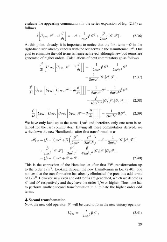
evaluate the appearing commutators in the series expansion of Eq. (2.34) asfollows

i[UFW,H − ih

∂∂ t

]=−O +

1mc2 βO2 +

β2mc2 [O,F ] . (2.36)

At this point, already, it is important to notice that the first term −O in theright-hand side already cancels with the odd terms in the Hamiltonian H . Ourgoal to eliminate the odd terms is hence achieved, although new odd terms aregenerated of higher orders. Calculations of next commutators go as follows

i2

2!

[UFW,

[UFW,H − ih

∂∂ t

]]=− 1

2mc2 βO2− 12m2c4 O3

− 18m2c4 [O, [O,F ]] , (2.37)

i3

3!

[UFW,

[UFW,

[UFW,H − ih

∂∂ t

]]]=

16m2c4 O3− 1

6m3c6 βO4

− β48m3c6 [O, [O, [O,F ]]] , (2.38)

i4

4!

[UFW,

[UFW,

[UFW,

[UFW,H − ih

∂∂ t

]]]]=

124m3c6 βO4 . (2.39)

We have only kept up to the terms 1/m3 and therefore, only one term is re-tained for the last commutator. Having all these commutators derived, wewrite down the new Hamiltonian after first transformation as

HFW = (β −�)mc2 +β(

O2

2mc2 −O4

8m3c6

)+E − 1

8m2c4 [O, [O,F ]]

+β

2mc2 [O,F ]− O3

3m2c4 −β

48m3c6 [O, [O, [O,F ]]]

= (β −�)mc2 +E ′+O ′ . (2.40)

This is the expression of the Hamiltonian after first FW transformation upto the order 1/m3. Looking through the new Hamiltonian in Eq. (2.40), onenotices that the transformation has already eliminated the previous odd termsof 1/m0. However, new even and odd terms are generated, which we denote asE ′ and O ′ respectively and they have the order 1/m or higher. Thus, one hasto perform another second transformation to eliminate the higher order oddterms.

♣ Second transformation

Now, the new odd operator, O ′ will be used to form the new unitary operator

U ′FW =− i

2mc2 βO ′ , (2.41)

29

where the odd operators are collected from Eq. (2.40) as

O ′ =β

2mc2 [O,F ]− O3

3m2c4 −β

48m3c6 [O, [O, [O,F ]]] . (2.42)

Following the similar prescription, after the second transformation the Hamil-tonian becomes

H ′FW = HFW + i

[U ′

FW,HFW− ih∂∂ t

]+

i2

2!

[U ′

FW,

[U ′

FW,HFW− ih∂∂ t

]]

+i3

3!

[U ′

FW,

[U ′

FW,

[U ′

FW,HFW− ih∂∂ t

]]]+ .... . (2.43)

With the help of the new unitary operator in Eq. (2.41) and the first transformedHamiltonian in Eq. (2.40), we have to evaluate the further commutators thatare involved in the second transformation i.e., Eq. (2.43). We keep the termsonly up to the order 1/m3, while the higher order terms have been dropped.Considering that, the commutators can be evaluated as

i[U ′

FW,HFW− ih∂∂ t

]

=− β2mc2 [O,F ]+

13m2c4 O3 +

β48m3c6 [O, [O, [O,F ]]]

− β8m3c6

{[O,F ] ,O2}− i

6m4c8 O5− β4m3c6 [O,F ]2

+1

4m2c4 [[O,F ] ,F ]− β6m3c6

[O3,F

], (2.44)

i2

2!

[U ′

FW,

[U ′

FW,HFW− ih∂∂ t

]]=

β8m3c6 [O,F ]2 . (2.45)

The higher order commutators have the order of 1/m4 or more and therefore,those are not taken into consideration further. After the second transformation,the new transformed Hamiltonian is written as

H ′FW = (β −�)mc2 +β

(O2

2mc2 −O4

8m3c6

)+E − 1

8m2c4 [O, [O,F ]]

− β8m3c6 [O,F ]2− β

8m3c6

{[O,F ] ,O2}+ 1

4m2c4 [[O,F ] ,F ]

− β6m3c6

[O3,F

]= (β −�)mc2 +E ′′+O ′′ . (2.46)

Note that, the odd terms have been eliminated up to the order 1/m2 in theabove Hamiltonian. However, by doing so, the new odd terms have been gen-erated and those are of higher orders i.e., 1/m3 or more. The newly generatedeven and odd terms are denoted as E ′ and O ′.

30

♣ Third transformation

Following the same procedure, a new odd operator O ′′ is formed so that thecorresponding unitary operator is given by

U ′′FW =− i

2mc2 βO ′′ , (2.47)

where the odd operator can be expressed as,

O ′′ =− β8m3c6

{[O,F ] ,O2}+ 1

4m2c4 [[O,F ] ,F ]− β6m3c6

[O3,F

].

(2.48)

Notice that the newly formed odd operator has already the order 1/m3 or more.This indicates that less commutators have to be evaluated as we restrict theseries only up to 1/m3. In fact, only the following commutator will contributeas,

i[U ′′

FW,H ′FW− ih

∂∂ t

]

=β

8m3c6

{[O,F ] ,O2}− 1

4m2c4 [[O,F ] ,F ]+β

6m3c6

[O3,F

]+

β8m3c6 [[[O,F ] ,F ] ,F ] . (2.49)

The evaluation of the other commutators results in the terms of order 1/m4 ormore and those are dropped. The newly transformed Hamiltonian is given as

H ′′FW = (β −�)mc2 +β

(O2

2mc2 −O4

8m3c6

)+E − 1

8m2c4 [O, [O,F ]]

− β8m3c6 [O,F ]2 +

β8m3c6 [[[O,F ] ,F ] ,F ]

= (β −�)mc2 +E ′′′+O ′′′ . (2.50)

At this point, one can notice that only the last term in the Hamiltonian of Eq.(2.50) is odd, all the rest have already been transformed to be even.

♣ Fourth transformation

A further transformation is needed as we see that the new odd operator, O ′′′ isformed. The new unitary operator is given as

U ′′′FW =− i

2mc2 βO ′′′ , (2.51)

with

O ′′′ =β

8m3c6 [[[O,F ] ,F ] ,F ] . (2.52)

31

The commutator that contributes, is evaluated as,

i[U ′′′

FW,H ′′FW− ih

∂∂ t

]=− β

8m3c6 [[[O,F ] ,F ] ,F ] , (2.53)

that is odd. Notice that, this term exactly cancels with the existing odd term inEq. (2.50). Hence, the final transformed Hamiltonian will be given as

H ′′′FW = (β −�)mc2 +β

(O2

2mc2 −O4

8m3c6

)+E − 1

8m2c4 [O, [O,F ]]

− β8m3c6 [O,F ]2 . (2.54)

This is the correct form of the FW transformed Hamiltonian up to the order1/m3 and we see that all the terms are even. The odd operators up to the sameorder are eliminated, in addition, the higher orders are neglected. This gives asemirelativistic expression where the zeroth order Hamiltonian reveals exactlythe Schrödinger Hamiltonian. Comparing with the Dirac Hamiltonian for acrystal, O = cααα · ppp and E = V , the crystal potential, the second and fourthterm of Eq. (2.54) lead to the kinetic and potential energies of the Schrödingerequation.

This method of the FW transformed Hamiltonian was proposed by using“step-by-step” transformations or an iterative method and calculating the com-mutators. Although Foldy and Wouthuysen took the weak fields into account,the higher orders are of doubtful value. In fact, they derived only the first or-der relativistic correction terms i.e., up to the terms 1/m2 for spin-1

2 particlestrictly [71]. The calculations of second and higher order terms do not deriveall the necessary relativistic correction terms. Therefore, a correction in FWtransformation is needed. We mention that, in 1954, Case generalized the ideaof FW transformation and extended it to include particles with integral spin aswell as arbitrary half-integral spin [114]. Furthermore, the FW operators havebeen found for any arbitrary spin and it has been a research topic of currentinterest [115–117].

In the next section, we provide other methods to recover the correctionterms in higher order expansion of FW transformation.

2.4 Corrections to the FW transformationThe fact that the original FW transformation is based on a series expansion to-wards a semirelativistic Hamiltonian, renders the higher order terms of doubt-ful value. Furthermore, the original method fails when the relativistic correc-tions i.e., the higher orders diverge. Note that the exponential operator eiUFW

in each step of the FW transformation should have the property that it is oddand Hermitian [101, 118].

32

2.4.1 Eriksen’s methodIn 1958, Eriksen developed a general form of the unitary operator, UFW andsubsequently the FW transformation which is single step, not “step-by-step”.Within Eriksen’s method, the FW transformation can uniquely be defined if theexponential operator eiUFW is odd and Hermitian [101, 118]. These conditionsare equivalent to

βeiUFW = e−iUFWβ . (2.55)

Eriksen found an operator which is non-exponential in contrast to the originalFW transformation. The search for such an operator which commutes withH and it has eigenvalues either +1 or −1, results in a sign operator λ inthe following way λ = H√

H 2 . Thereby, the operator βλ or λβ are unitary

given the fact that λ 2 = 1. The operator 1+ βλ has the property that for βmatrix elements equal to 1 or -1, the operator cancels either the lower or uppercomponents of the Dirac spinor. Instead of an exponential operator, Eriksenproposed the following operator for an exact FW transformation [100, 101]

eiUFW = SFW =1+βλ√

2+βλ +λβ. (2.56)

It is appealing to test the convergence of the operator. Let us consider aneigenfunction, uδ of βλ such that βλuδ = eiδ uδ . From the left multiplyingwith e−iδ λβ in both the sides results in e−iδ uδ = λβuδ . Taking the sum ofboth we get

(βλ +λβ )uδ =(

eiδ + e−iδ)

uδ = 2cosδ uδ . (2.57)

The denominator in the Eriksen operator in Eq. (2.56) becomes

(2+βλ +λβ )uδ = 2(1+ cosδ )uδ . (2.58)

The convergence condition will be given by 2+ 2cosδ > 0 or cosδ > −1.A few other properties of the operator has to be noted: S2

FW = βλ , S†FW =

λβSFW and then SFWS†FW = 1. Once the Eriksen operator is constructed, it is

interesting to see whether the original FW transformation operator is achieved(see Appendix A for details).

The Eriksen operator for the FW transformation can be used for a particlewith any spin [100]. The FW transformation within Eriksen’s method will begiven as following for the time-independent case [101],

H ErikFW = SFWH S†

FW . (2.59)

Note that this transformation is not iterative because it does not involve theexponential operators, unlike the original FW transformation.

33

♣ Free Dirac particle

For a free Dirac particle, the following Eriksen operator is derived

λ =βmc2 +O√m2c4 +O2

, (2.60)

with the fact that E = 0 and O = cααα · ppp. Since, β and λH commute with eachother and λH = H λ , we get (1+βλ )H = H (1+λβ ). This implies thatH S†

FW = SFWH and the Eriksen condition is satisfied. The transformation inthis case is rather easy and will be given as

H ErikFW = SFWH S†

FW = S2FWH = βλH = β

√m2c4 +O2 . (2.61)

This result is exactly the same as the result presented in Sec. 2.3.3. Again, itis important to note that Eriksen’s method is not “step-by-step”, rather it is asingle transformation.

♣ Dirac particle in a potential

When a Dirac Particle experiences a potential then E �= 0. Thus, we have tocalculate the λ operator carefully, and that involves the determination of

√H 2

in the denominator. The latter will be written as√

H 2 =√

m2c4 +O2 +E 2 +2βmc2E +{O,E }

= βmc2

√1+

O2 +E 2 +2βmc2E +{O,E }m2c4 . (2.62)

Now this has to be expanded in a Taylor series and the transformation willhave the relativistic correction terms in the powers of O/m and E /m. The an-alytic expansion is non-trivial and rather cumbersome. However, by using ananalytic computer program E. de Vries and J. E. Jonker derived all the correctrelativistic terms up to the order 1/c8 [85]. To include the time dependency,one works with F = E − ih ∂

∂ t instead of E and finally the results up to theorder 1/m3 will be given in a compact form as [85, 100, 110]

H ErikFW = (β −�)mc2 +β

(O2

2mc2 −O4

8m3c6

)+E − 1

8m2c4 [O, [O,F ]]

+β

16m3c6 {O, [[O,F ] ,F ]} . (2.63)

Again, this approach does not need any subsequent iterations. Let us verifythe two Hamiltonians - one obtained by the original FW transformation inEq. (2.54) and the other obtained by Eriksen’s method in Eq. (2.63). All theHamiltonian terms are the same in both cases except the last term which hasthe order 1/m3c6. This proves that the original FW transformation does not

34

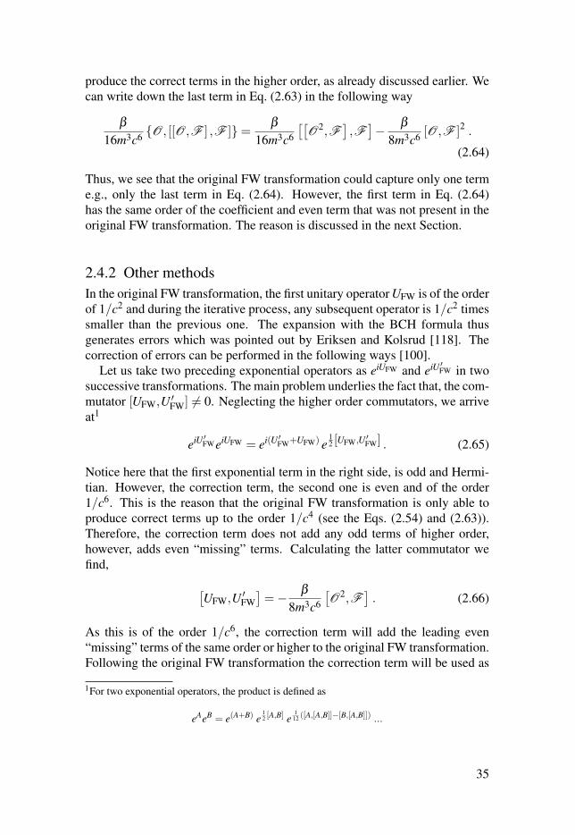
produce the correct terms in the higher order, as already discussed earlier. Wecan write down the last term in Eq. (2.63) in the following way

β16m3c6 {O, [[O,F ] ,F ]}= β

16m3c6

[[O2,F

],F

]− β8m3c6 [O,F ]2 .

(2.64)

Thus, we see that the original FW transformation could capture only one terme.g., only the last term in Eq. (2.64). However, the first term in Eq. (2.64)has the same order of the coefficient and even term that was not present in theoriginal FW transformation. The reason is discussed in the next Section.

2.4.2 Other methodsIn the original FW transformation, the first unitary operator UFW is of the orderof 1/c2 and during the iterative process, any subsequent operator is 1/c2 timessmaller than the previous one. The expansion with the BCH formula thusgenerates errors which was pointed out by Eriksen and Kolsrud [118]. Thecorrection of errors can be performed in the following ways [100].

Let us take two preceding exponential operators as eiUFW and eiU ′FW in twosuccessive transformations. The main problem underlies the fact that, the com-mutator [UFW,U ′

FW] �= 0. Neglecting the higher order commutators, we arriveat1

eiU ′FWeiUFW = ei(U ′FW+UFW) e12 [UFW,U ′FW] . (2.65)

Notice here that the first exponential term in the right side, is odd and Hermi-tian. However, the correction term, the second one is even and of the order1/c6. This is the reason that the original FW transformation is only able toproduce correct terms up to the order 1/c4 (see the Eqs. (2.54) and (2.63)).Therefore, the correction term does not add any odd terms of higher order,however, adds even “missing” terms. Calculating the latter commutator wefind,

[UFW,U ′

FW]=− β

8m3c6

[O2,F

]. (2.66)

As this is of the order 1/c6, the correction term will add the leading even“missing” terms of the same order or higher to the original FW transformation.Following the original FW transformation the correction term will be used as

1For two exponential operators, the product is defined as

eAeB = e(A+B) e12 [A,B] e

112 ([A,[A,B]]−[B,[A,B]]) ...

35

following:

H corrFW = e

12 [UFW,U ′FW]

(H ′′′

FW− ih∂∂ t

)e−

12 [UFW,U ′FW] + ih

∂∂ t

= H ′′′FW−

[12[UFW,U ′

FW],

(H ′′′

FW− ih∂∂ t

)]. (2.67)

Thus, the leading order correction will be the given by the commutator,[12[UFW,U ′

FW],E − ih

∂∂ t

]=− β

16m3c6

[[O2,F

],F

]. (2.68)

This is exactly the “missing” even term, that was not obtained by the originalFW transformation (see Eq. 2.64). Hence, we have shown that up to an order1/c6, the Eriksen method and the corrected FW method result in the sametransformed Hamiltonian i.e.,

H corrFW = H Erik

FW . (2.69)

For the higher orders, one needs to take into account the other commutatorsfor corrections e.g., [UFW,(U ′

FW +U ′′FW)] (see Ref. [100] for details).

To summarize, the original iterative method proposed by Foldy and Wouthuy-sen [71] does not produce all the correct even terms in higher order and there-fore it is not trustworthy. The fact that the different unitary operators do notcommute with each other leads to the “missing” even terms in the original FWtransformation. The correct FW transformation can be achieved by two meth-ods that are described above. One of them is to consider the corrected evenoperator in each iterative process that will produce the missing even terms inthe first place. On the other hand, Eriksen’s method is not iterative rather a sin-gle step towards the direct FW transformation and can capture all the higherorder even relativistic terms. However, the Eriksen method cannot be used inpractical purposes because it involves the square root of different Dirac ma-trices (see Eqs. (2.56), (2.62)). Thus, the most applied methods are based onthe correction of the FW transformation and the use of exponential operators.The intermediate operators in the successive transformations are odd and Her-mitian in the FW transformation. However, the correction operators are evenand Hermitian, and compensate with the “missing” terms in the original FWtransformation. Let us also mention that the series obtained by semirelativisticmethods diverge when p > mc [100, 111, 117].

Once we have all the relativistic correction terms to the nonrelativistic Pauli-Schrödinger Hamiltonian, we apply those terms in more physical (e.g., mag-netic) systems in the next Section.

36

♣ Summary of FW transformationThe unitary operators and the corresponding Hamiltonians in each steps of theoriginal TDFW transformation are given below (these are in agreement withRef. [100]):

UFW =− i2mc2 βO

HFW = (β −�)mc2 +β(

O2

2mc2 −O4

8m3c6

)+E − 1

8m2c4 [O, [O,F ]]

+β

2mc2 [O,F ]− O3

3m2c4 −β

48m3c6 [O, [O, [O,F ]]]

U ′FW =− i

4m2c4 [O,F ]+iβ

6m3c6 O3 +i

96m4c8 [O, [O, [O,F ]]]

H ′FW = (β −�)mc2 +β

(O2

2mc2 −O4

8m3c6

)+E − 1

8m2c4 [O, [O,F ]]

− β8m3c6 [O,F ]2− β

8m3c6

{[O,F ] ,O2}+ 1

4m2c4 [[O,F ] ,F ]

− β6m3c6

[O3,F

]U ′′

FW =i

16m4c8

{[O,F ] ,O2}− iβ

8m3c6 [[O,F ] ,F ]+i

12m4c8

[O3,F

]H ′′

FW = (β −�)mc2 +β(

O2

2mc2 −O4

8m3c6

)+E − 1

8m2c4 [O, [O,F ]]

− β8m3c6 [O,F ]2 +

β8m3c6 [[[O,F ] ,F ] ,F ]

U ′′′FW =− i

16m4c8 [[[O,F ] ,F ] ,F ]

H ′′′FW = (β −�)mc2 +β

(O2

2mc2 −O4

8m3c6

)+E − 1

8m2c4 [O, [O,F ]]

− β8m3c6 [O,F ]2

H ErikFW = (β −�)mc2 +β

(O2

2mc2 −O4

8m3c6

)+E − 1

8m2c4 [O, [O,F ]]

+β

16m3c6 {O, [[O,F ] ,F ]}= H corr

FW

37

2.5 FW transformation for a magnetic solid in anelectromagnetic field

We have already pointed out that the free particle Dirac Hamiltonian is givenby the Eq. (2.6). Such a theory has been used to describe the ground stateproperties of any system by using the concept of particle density, n(rrr) in DFT[66, 67]. To describe a relativistic particle within relativistic DFT, the Dirac-Kohn-Sham (DKS) Hamiltonian is written as [70, 119, 120]

H KSD = cααα · (ppp− eAAAeff)+βmc2 +Veff , (2.70)

where the effective scalar and vector potentials are the functions of externalpotentials, exchange-correlation energies [121]. To account for the magneticsolids, the magnetic exchange interaction is of particular interest as the ex-change interaction can give rise to an exchange field of the order of 103 T.The magnetic exchange interaction arises due to the Pauli exclusion principlewhich says that two electrons with same spin cannot have the same ‘position’in a specific orbital. The exchange interaction is responsible for the differenttypes of spontaneous ordering of atomic magnetic moments occurring in mag-netic solids e.g., ferromagnetism, antiferromagnetism and ferrimagnetism.

The detailed discussion of different exchange interactions are beyond thescope of this thesis, however, we stress the point that the corresponding ex-change field, BBBxc is different from the one of usual Maxwell’s fields, or inother words, BBBxc does not obey the Maxwell’s equations [122]. The reasonis because BBBxc couples only to the spin degrees of freedom, not to the otherdegrees of freedom [122]. Thus, this field is not a proper magnetic field andcannot be included as a vector potential, AAAxc. Instead, we have to treat theeffect of exchange field in a separate term within the DKS Hamiltonian asfollows [123, 124]

HDKS = cααα · (ppp− eAAA)+(β −�)mc2 +V + eΦ−μBβΣΣΣ ·BBBxc . (2.71)

The electromagnetic field is taken care by the vector potential as minimal cou-pling and scalar potential energy eΦ, V defines the unpolarized crystal po-tential and the exchange field is separately accounted. Now, following thedescription of the FW transformation, the Hamiltonian in Eq. (2.71) containsodd terms and even terms. The Dirac matrices ααα have off-diagonal elementsin the matrix formalism and therefore, they form odd operators and β containsdiagonal elements constructing even operators. Following Eq. (2.71), the oddand even operators can be written as below

O = cααα · (ppp− eAAA) , (2.72)E =V + eΦ−μBβΣΣΣ ·BBBxc . (2.73)

Therefore, the Hamiltonian can be expressed as in the form of Eq. (2.17).As the vector potential, AAA(rrr, t) depends on time, a TDFW transformation is

38

performed for the separation of particles from antiparticles. The next step willbe to substitute these odd and even operators in Eq. (2.63) and calculate theHamiltonian. The corrected FW transformation gives the Hamiltonian termsdiscussed further below, which describe spin- 1

2 particles.Putting together all the derived Hamiltonian terms, we write down the ex-

tended Pauli Hamiltonian including the relativistic effects up to an order of1/c4:

H extn.Pauli =

=(ppp− eAAA)2

2m+V + eΦ−μB σσσ · (BBB+BBBxc

)︸ ︷︷ ︸

Pauli Hamiltonian

− (ppp− eAAA)4

8m3c2︸ ︷︷ ︸mass correction

+eh

8m3c2

{(ppp− eAAA)2 ,σσσ ·BBB}︸ ︷︷ ︸

indirect field−spin coupling

− eh2

8m2c2 ∇∇∇ ·EEE tot︸ ︷︷ ︸Darwin term

− eh8m2c2 σσσ ·

[EEE tot× (ppp− eAAA)− (ppp− eAAA)×EEE tot

]︸ ︷︷ ︸

spin−orbit and spin−photon coupling

+μB

8m2c2 σσσ ·BBBxccorr +

iμB

4m2c2 [(ppp×BBBxc) · (ppp− eAAA)]︸ ︷︷ ︸relativistic corrections to the exchange field

− ieh2

16m3c4 σσσ · [∂tEEE tot× (ppp− eAAA)+(ppp− eAAA)×∂tEEE tot]︸ ︷︷ ︸higher−order spin−orbit coupling

(2.74)

These relativistic Hamiltonian terms seems to be complicated, however,their physical meanings are immediately explained.

2.5.1 Pauli HamiltonianThe second and fourth terms in Eq. (2.63) constitute the nonrelativistic PauliHamiltonian, however, yet including the magnetic exchange field. The PauliHamiltonian is written as,

HP =(ppp− eAAA)2

2m+V + eΦ−μB σσσ ·BBB−μB σσσ ·BBBxc, (2.75)

where the external magnetic field is given by BBB = ∇∇∇×AAA and μB = eh2m , defines

the Bohr magneton. The last two terms of the Pauli Hamiltonian explains theZeeman coupling with the external magnetic field and exchange field respec-

39

tively. We choose for simplicity a gauge such that

AAA =BBB× rrr

2, (2.76)

which fulfills the Coulomb gauge (∇∇∇ ·AAA = 0) for the uniform magnetic field2.It is important to note that with this Pauli Hamiltonian one can show how thedifferent magnetic contributions arise. Incorporating the gauge choice, thePauli Hamiltonian can be rewritten as

HP =

(p2

2m+V

)+ eΦ− e

mBBB · (LLL+gSSS)+

e2

8m(BBB× rrr)2− e

mSSS ·BBBxc , (2.77)

with g the Landé g-factor, which is approximately 2 for spin degrees of free-dom. The spin angular momentum is represented by SSS = h

2 σσσ and the orbitalangular momentum is defined by LLL = rrr× ppp. The first term of Eq. (2.77) is ob-viously the unperturbed Hamiltonian - the Schrödinger terms, the third term isthe dominant perturbation - the paramagnetic contribution and the fourth termis recognized as the diamagnetic contribution [125].

Note that, the external magnetic field couples to both the spin and the orbitalangular momentum operators, as it should be. However, the exchange fieldonly couples to the spin degrees of freedom as discussed earlier.

2.5.2 Relativistic mass correctionThe very first relativistic correction appears in the form of relativistic masscorrection that is derived from the third term of Eq. (2.63) as

HRMC =−(ppp− eAAA)4

8m3c2 . (2.78)

In the same context, we note that in special relativity, the mass correctionarises from the relativistic momentum-energy relation in Eq. (2.2) such as

E = mc2(

1+p2

m2c2

) 12

≈ mc2 +p2

2m− p4

8m3c2 . (2.79)

As the relativistic mass correction does not concern us about the electron spin,this will not be considered in our discussions in this thesis which will mostlyfocus on the magnetic systems. The expansion of third term of Eq. (2.63)includes two more terms but those belong to the indirect field-spin coupling[90]. The spin dependent indirect field-spin coupling term is derived as

Hindirect =eh

8m3c2

{(ppp− eAAA)2 ,σσσ ·BBB} . (2.80)

2 ∇∇∇×AAA = 12 ∇∇∇× (BBB× rrr) = 1

2 [BBB(∇∇∇ · rrr)− rrr(∇∇∇ ·BBB)+(rrr ·∇∇∇)BBB− (BBB ·∇∇∇)rrr] = 12 [3BBB−BBB] = BBB

∇∇∇ ·AAA = 12 ∇∇∇ · (BBB× rrr) = (∇∇∇×BBB) · rrr−BBB · (∇∇∇× rrr) = 0

40

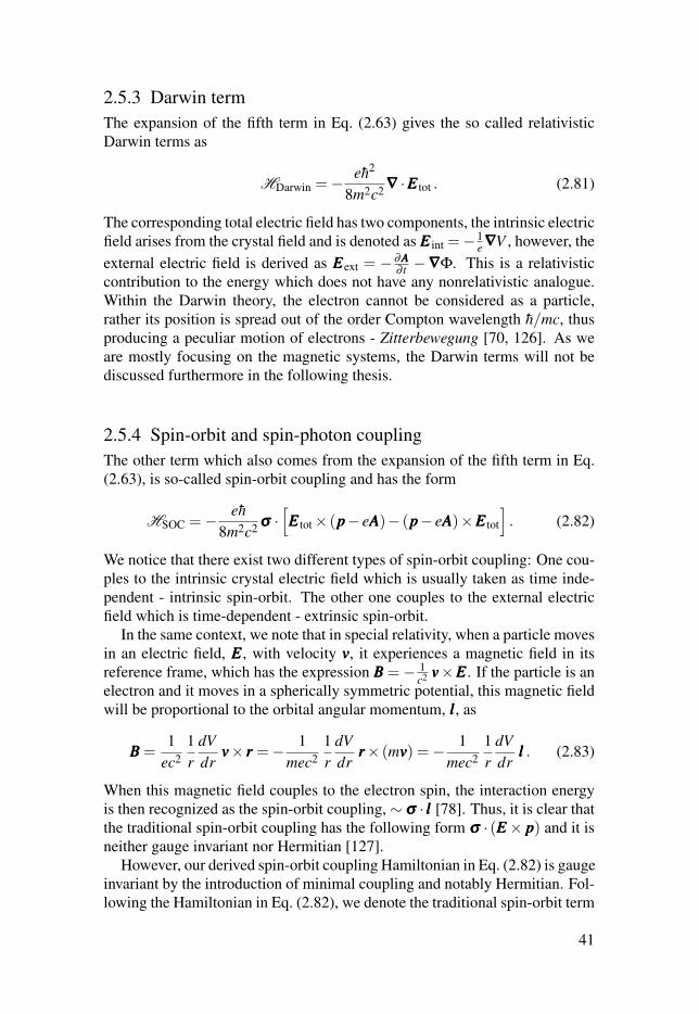
2.5.3 Darwin termThe expansion of the fifth term in Eq. (2.63) gives the so called relativisticDarwin terms as

HDarwin =− eh2

8m2c2 ∇∇∇ ·EEE tot . (2.81)

The corresponding total electric field has two components, the intrinsic electricfield arises from the crystal field and is denoted as EEE int =−1

e ∇∇∇V , however, theexternal electric field is derived as EEEext = −∂AAA

∂ t −∇∇∇Φ. This is a relativisticcontribution to the energy which does not have any nonrelativistic analogue.Within the Darwin theory, the electron cannot be considered as a particle,rather its position is spread out of the order Compton wavelength h/mc, thusproducing a peculiar motion of electrons - Zitterbewegung [70, 126]. As weare mostly focusing on the magnetic systems, the Darwin terms will not bediscussed furthermore in the following thesis.

2.5.4 Spin-orbit and spin-photon couplingThe other term which also comes from the expansion of the fifth term in Eq.(2.63), is so-called spin-orbit coupling and has the form

HSOC =− eh8m2c2 σσσ ·

[EEE tot× (ppp− eAAA)− (ppp− eAAA)×EEE tot

]. (2.82)

We notice that there exist two different types of spin-orbit coupling: One cou-ples to the intrinsic crystal electric field which is usually taken as time inde-pendent - intrinsic spin-orbit. The other one couples to the external electricfield which is time-dependent - extrinsic spin-orbit.

In the same context, we note that in special relativity, when a particle movesin an electric field, EEE, with velocity vvv, it experiences a magnetic field in itsreference frame, which has the expression BBB =− 1

c2 vvv×EEE. If the particle is anelectron and it moves in a spherically symmetric potential, this magnetic fieldwill be proportional to the orbital angular momentum, lll, as

BBB =1

ec21r

dVdr

vvv× rrr =− 1mec2

1r

dVdr

rrr× (mvvv) =− 1mec2

1r

dVdr

lll . (2.83)

When this magnetic field couples to the electron spin, the interaction energyis then recognized as the spin-orbit coupling, ∼ σσσ · lll [78]. Thus, it is clear thatthe traditional spin-orbit coupling has the following form σσσ · (EEE× ppp) and it isneither gauge invariant nor Hermitian [127].

However, our derived spin-orbit coupling Hamiltonian in Eq. (2.82) is gaugeinvariant by the introduction of minimal coupling and notably Hermitian. Fol-lowing the Hamiltonian in Eq. (2.82), we denote the traditional spin-orbit term

41

as σσσ · (EEE tot× ppp), however, the spin-photon coupling as σσσ · (EEE tot×AAA). Alter-natively, we mention that such spin-orbit coupling terms can also be derivedusing Møller’s idea in special relativity together with the Schrödinger Hamil-tonian [128].

Throughout this thesis, we will show that the relativistic spin-orbit and spin-photon coupling is very much important in explaining many complex physicalphenomena in condensed matter magnetic systems.

2.5.5 Relativistic corrections to the exchange fieldThe fifth term in Eq. (2.63) also provides the derivation of relativistic correc-tions to the exchange field while considering the exchange field as the eventerms in the FW transformation. These terms can be written as3

HRCXC =μB

8m2c2 σσσ ·{[

p2BBBxc]+2(pppBBBxc)·(ppp− eAAA)+2(ppp ·BBBxc)(ppp− eAAA)

+4[BBBxc·(ppp− eAAA)](ppp− eAAA)}+

iμB

4m2c2 [(ppp×BBBxc) · (ppp− eAAA)] . (2.84)

The terms within {} can be recognized as the effective Zeeman-like field dueto the exchange field which are relativistic corrections, they can be written as

BBBxccorr =

[p2BBBxc

]+2(pppBBBxc)·(ppp− eAAA)+2(ppp ·BBBxc)(ppp− eAAA)

+4[BBBxc·(ppp− eAAA)](ppp− eAAA) . (2.85)

These terms can be explained as the spin-orbit coupling due to the exchangefield. This is more apparent with the substitution of momentum operatorsin the Eq. (2.84) as radial and angular parts: ppp = eeer pr − rrr×LLL

r , where pr =−ih∂/∂ r is the radial part of the momentum operator and eeer is the unit radialvector. As the exchange fields are usually very strong for magnetic systems(ferromagnets), their relativistic corrections cannot be ignored at all.

Apart from the last term in Eq. (2.84), as pointed out, the rest can be writtentogether to form an effective exchange correction field as BBBxc

corr and the samecan be re-written as

HRCXC =μB

8m2c2 σσσ ·BBBxccorr +

iμB

4m2c2 [(ppp×BBBxc) · (ppp− eAAA)] . (2.86)

Notice that, these terms contain all the informations of the interaction amongthe spins, the electromagnetic fields and the exchange fields. We also state thatthe inclusion of BBBxc in the Dirac equation is not the same as the inclusion in the

3The following vector identity is used for any three vectors aaa, bbb and ccc

(σσσ ·aaa)(σσσ ·bbb)(σσσ · ccc) = (σσσ ·aaa)(bbb · ccc)+(aaa ·bbb)(σσσ · ccc)−aaa(σσσ ·bbb) · ccc+ i(aaa×bbb) · ccc

42

Pauli equation. There have been attempts to derive the relativistic correctionterms of exchange fields, however, only a component of the exchange fieldwas used [86]. Here, in our derivation, we use a general exchange field anduse the corrected FW transformation to obtain the relativistic correction terms- this has not been done before.

2.5.6 Higher-order spin-orbit couplingThe last term of Eq. (2.63) is a higher order in the transformation as it is ofthe order 1/c6. The expansion of the last term gives the Hamiltonian which isrecognized as the higher order spin-orbit coupling that takes the form,

H higherSOC =− ieh2

16m3c4 σσσ · [∂tEEE tot× (ppp− eAAA)+(ppp− eAAA)×∂tEEE tot] . (2.87)

Note that, the difference between Eq. (2.82) and Eq. (2.87) are: (i) the latteris 1

c2 times smaller than the usual spin-orbit coupling Hamiltonian and (ii)a first-order time-derivative of the electric field is present in the latter onewhile no time-derivative is involved in the usual spin-orbit coupling. But it isinteresting that both of them have similar formulation and they are Hermitianand gauge invariant. The intrinsic electric field is time independent, thus, theircontributions will be zero in the higher-order spin-orbit coupling, restrictingto the external electric field which only contributes. These higher order spin-orbit coupling have not often been discussed in the literature but they can havemuch importance as well [90]. We note that, the expansion of the last term inEq. (2.63) further gives another term which is spin independent and thus wedo not intend to it include here [90].

To summarize, we have used the DKS Hamiltonian in an electromagneticenvironment, however, treated the exchange field separately. Using the cor-rected FW transformation, we have derived the extended Pauli Hamiltonianthat includes all the relativistic correction terms up to an order 1/c4. In thenext chapters, we will describe how these derived terms contribute to manyphysical phenomena in magnetic systems.

43

3. Magnetization Dynamics: Precession,Damping, Nutation, Torque

3.1 IntroductionMagnetism was known since ancient ages; it was probably the ancient Greekswho first reflected upon the unusual properties of magnetite (iron ore) [129]. Itwas used in devices, for example the most common use were the compasses innavigation. Despite of being used in the ancient times, the fundamental originof magnetism in a material was mysterious and concealed. In the middle of19th century James Clerk Maxwell compiled the theory of electromagnetism,which was the greatest step in explaining the electricity and magnetism [78].In particular, the Maxwell equations establish a relationship between the elec-tric systems (charge density and electric field) and the magnetic systems (cur-rent density and magnetic field) and they describe how the change of electricfield produces a magnetic field and vice-versa. These equations provide thecornerstone for understanding electromagnetic phenomena and are even heav-ily used today [130].

Although magnetism and electricity can be expressed through the Maxwellequations, the origin of spontaneous magnetism (presence of magnetic fieldwithout any application of an electric field) in some materials cannot be un-derstood from the Maxwell equations. To this end, the analysis of magnetismfrom a quantum theory is required. Here, in the following, first the classi-cal theory of magnetic moment is given, followed by the quantum theory andtheory of magnetic ordering.

3.2 Magnetic momentIn the classical theory of electromagnetism, when a charged particle movesin a current loop, it produces a magnetic dipole moment. The magnitude ofthe moment is proportional to the amount of current and the area of the loop.Similarly, when the electron orbits around a nucleus (atom), it gives rise toan angular momentum. The Einstein-de Haas effect1 could explain that mag-netism is related to angular momentum, specifically, the magnetic moment isproportional to the angular momentum of the orbiting electron as

μμμe =e

2mLLL . (3.1)

1A freely unmagnetized suspended rod starts to rotate to compensate the angular momentumwhen a magnetic field is induced in it.

45

The orbital angular momentum of the electron is LLL = rrr× ppp and due to thenegative electronic charge, e = −|e|, the magnetic moment and the angularmomentum are antiparallel to each other [125].

However, the classical explanation of arising magnetic moment is not suf-ficient, because of the following reasoning. The partition function (describesthe statistical properties e.g., energy, entropy etc. of a system under thermo-dynamic equilibrium) of N classical particles each of charge q can be writtenas

Z =

∫ ∫...∫

Exp[− E{rrri, pppi}

kBT

]drrr1drrr2...drrrN d ppp1d ppp1...d pppN , (3.2)

where E{rrri, pppi} is the energy associated to the N charged particles with posi-tions and momentum rrri and pppi respectively. When a magnetic field (definedby the vector potential AAA(rrr, t)) is applied to the system, the momentum getschanged by pppi → (pppi− eAAA) (see the end of Sec. 2.2.1). Therefore the freeenergy of the system, F =−kBT logZ is not a function of magnetic field. Thecorresponding magnetization is MMM = −∂F/∂HHH is then expected to be zero,which indicates that considering the ensemble of classical charged particles,one cannot explain the spontaneous magnetization of materials. The afore-mentioned statement is known as Bohr van-Leeuwen theorem. The theoremjustifies that the magnetic properties of materials can be properly accountedonly when we go beyond classical physics, into quantum mechanics.

The intrinsic property of an electron is spin, a purely quantum mechani-cal concept. The electrons not only move in an orbit around the nucleus, butalso precess around their own axes, leading to the origin of spin angular mo-mentum. For electrons, the spin quantum number, s takes the value 1

2 and thespin algebra is connected to the Pauli spin matrices σσσ = (σx, σy, σz) in spinorspace. The spin angular momentum is then denoted by SSS = h

2 σσσ . Similar to Eq.(3.1), the spin moment is expressed as

μμμs = ge

2mSSS , (3.3)

where g≈ 2, is the Landé g-factor for electrons.The values of any component of spin angular momentum are discrete and

can take only one of the 2s+ 1 values, provided that the normal componentis determined by the quantum number ms = ±1

2 (corresponding to spin upand spin down). This is in accordance with the orbital angular momentumwhich can also take any of 2l + 1 values, where the orbital quantum numberis l and the z-components are determined by ml = ±l,±(l − 1) and so on.The magnitude of the total spin angular momentum for atoms with severalelectrons is found as S = ∑ms, while the orbital angular momentum is L =

∑ml . The total magnetic moment is then the sum of the orbital contributionand the spin contribution.

For determining the total moments of electrons on atoms the filling of elec-tron shells is important. These values of the moment and angular momentum

46

Figure 3.1. Hund’s rules for the electrons in a d orbital. S, L and J represent the spin,orbital and total angular momentum, respectively. A d orbital can contain a maximumof 10 electrons. According to the Hund’s rule, the filling of electrons in the availableshells dictates the angular momentum in the ground state configuration.

can be calculated from the ground of the electronic configuration of an atom.The ground state can be obtained from the Hund’s rules that have three mainstatements:(a) Maximize S: this means the spin up electrons will be arranged first in theavailable shells and then the spin down, or the other way around. For ex-ample, if there are two electrons, the total spin angular momentum will beS = 1/2+1/2 = 1. The blue plot in Fig. 3.1 refers to such an arrangement ford orbital (l = 2).(b) Maximize L: this means once S is maximized, the choice of l has to besuch that L is maximized. For example, a d orbital has the z-component ofangular momentum as ml =±2,±1,0 and therefore for two electrons the val-ues of ml is chosen as +2 and +1 so that the total orbital angular momentumis L = 2+ 1 = 3. The red plot in Fig. 3.1 refers to such an arrangement forelectrons filling the d orbital.(c) Maximize J: this means if the shell is more than half-filled, the total angu-lar momentum is taken as J = L+ S, otherwise, the total angular momentumcan be calculated as J = L−S. For example, the d orbital can have maximumof 10 electrons, therefore the availability of two electrons follows the less thanhalf filled arrangement. The total angular momentum will be J = 3− 1 = 2.The green plot in Fig. 3.1 refers to such an arrangement for the d orbital.

Therefore, using the Hund’s rules, one can conclude that the partially filledshells give rise to nonzero magnetic moment in the ground state and thus canexplain the origin of magnetism.

47

♣Magnetic ordering

Depending on the orientation of the magnetic moments, the magnetic sys-tems can be classified into mainly three classes: ferromagnet, antiferromagnetand ferrimagnet. The ferromagnetic order is obtained when the magnetic mo-ments are aligned in parallel to each other, producing a finite (nonzero) valueof net magnetization. The antiparallel alignment of the magnetic momentsgives rise to the antiferromagnetic orders resulting a net zero magnetization.The ferrimagnetic order arises when the magnetic moments are antiparallel toeach other but the magnitude of the magnetic moments are not equal. As aconsequence, the net magnetization is nonzero. Apart from these three usualmagnetic ordering, there exist many complex orders such as the noncollinearmagnetic moments.

Microscopically, the ordered magnetic structure is the result of correlationamong the direction of electrons (spins). This correlation is due to the fact thatthe space symmetry of the wave function depends on the magnitude of the re-sultant spin of the system of electrons. Thus, different values of the energy ofthe system in general correspond to wave functions with different space sym-metry. This effect is called exchange effect and the dependence of energy onthe magnitude of spins i.e., the dependence of energy on the symmetry proper-ties of the wave functions, is referred to as being due to the exchange interac-tions. The exchange interaction is mainly responsible for the long-range orderin a ordered magnetic structure. The exchange interaction can be modeled bythe Hamiltonian following the simple Heisenberg prescription [125, 131].

3.3 MagnetizationThe magnetization is defined by the magnetic moment per unit volume. There-fore, one must take the expectation value of the total magnetic moment μμμ as[131]

MMM =∫

ψ�μμμψ ∏i

drrri , (3.4)

where ψ is a many-body wave function. But, the main problem lies with thefact that the exact many-body wave function is never known for a particularsystem. To approximate it, one introduces a set of eigenfunctions of the sys-tem so that the wave function can be written in a superposition of the eigenfunctions (φk) of the system as ψ(rrr1,rrr2, ...,rrrN , t) = ∑k ak(t)φk(rrr1,rrr2, ...,rrrN).The magnetization can then be recast as

MMM(rrr, t) = ∑k,k′

a�k(t)ak′(t)μμμkk′ , (3.5)

where μμμkk′ defines the magnetic moment matrix elements. Finally, taking atime-average and realizing the fact that the statistical density matrix ρkk′ =

48

a�k(t)ak′(t), the magnetization of the entire system becomes

MMM = Tr [ρμμμ] . (3.6)

However, if one is interested in defining a magnetization at the point rrr, wehave to introduce the magnetic moment density as follows

μμμ(rrr) =12 ∑

j

[μμμ j δ (rrr− rrr j)+δ (rrr− rrr j)μμμ j

]. (3.7)

For the orbital moment, as it is a function of position and momentum opera-tor, the symmetrized expression has been used. But, for the spin moment, thesymmetric product is not mandatory because the spin moment and the den-sity operator commute with each other. Note that, the δ -function defines thedensity operator which has the dimension of inverse volume. For a strong fer-romagnet, the orbital moment is usually quenched because of the cubic crystalfield and the magnetization is largely given by the spin moment only. Thus,throughout the dynamics, we consider the spin moments, the orbital momentsare ignored. However, it is important to note that a full magnetization de-scription, including orbital and spin contributions, is necessary to describe thedynamics for other systems (e.g., lanthanides). We write the magnetization as

MMM(rrr, t) =gμB

h ∑j

Tr [ρ SSS j δ (rrr− rrr j)] , (3.8)

where μB is the Bohr magneton which serves as a unit of the magnetic mo-ment. Once the magnetization is defined for a system, the magnetization dy-namics can be analyzed appropriately.

3.4 Magnetization dynamicsThe time evolution of a magnetization element has been successfully describedwithin the phenomenological Landau-Lifshitz (LL) equation of motion [37].The corresponding dynamics involves a precession of the magnetization vectoraround an effective field and a subsequent transverse relaxation of magnetiza-tion that is called damping. Because of the form of the transverse damping, themagnitude of the magnetization does not change during the LL dynamics. Theproposed phenomenological LL equation for a magnetization element, MMM(rrr, t)(magnetic moment per unit volume at each point) is defined as

∂MMM∂ t

=−γMMM×HHHeff−λMMM× (MMM×HHHeff) , (3.9)

where γ is the gyromagnetic ratio, HHHeff is the effective magnetic field andλ is the scalar isotropic damping parameter that dictates the rate at which

49

M

Heff

M ×Heff

M × ∂M∂tPrecession

Damping

Figure 3.2. Magnetization dynamics has been schematically depicted. The red ar-row shows the magnetization vector. It precesses around the effective field and thedamping curves are shown in red color as well.

the z-magnetization direction is dissipated. The effective field includes theexternally applied field, demagnetizing field, magnetocrystalline anisotropy,spin-spin exchange interaction etc. [132, 133].

However, to include the effect of large (anomalous) damping for real fer-romagnets, Gilbert modified the preexisting LL equation, accounting for theGilbert damping parameter α in the Landau-Lifshitz-Gilbert (LLG) dynamics[38–40]

∂MMM∂ t

=−γ ′MMM×HHHeff +αMMM× ∂MMM∂ t

. (3.10)

This LLG equation of motion can be re-written in the form of LL dynamicsand both the LL and LLG equations are shown to be mathematically equivalentto each other with the fact that γ = γ ′/(1+α2M2) and λ = αγ ′/(1+α2M2).The corresponding two dynamics (precession and transverse damping) areschematically depicted in the Fig. 3.2. Originally the damping parameterswere attributed to the relativistic origins and predicted to be scalar quantities[37].

For practical purposes, the extension to the LLG equation has been useful todescribe several other dynamical effects. For example, to include the effect ofmagnetic inertia (spin nutation), the LLG equations have been extended withan inertia term. Nutation means a continuous change of the precession angleof the magnetization vector while it precesses around an effective field. Thiseffect has been predicted to be observed in ultrashort timescales i.e., sub-ps[134, 135]. While the Gilbert damping effect enters into the LLG equationas a first order time-derivative of the magnetization, the nutation dynamics hasbeen related to the second order time-derivative of the magnetization [42, 135].

50

Another extension of the LLG equation is to include the effect of spin cur-rents, which naturally appear in the spin continuity equation [43, 44]. Thesespin currents can be of nonrelativistic and of relativistic origin. By includ-ing the effect of spin currents in the extended LLG equation, it is possibleto describe phenomenologically the current induced phenomena such as spin-transfer torque, spin-orbit torque etc.

The derivations of the LLG equations and their extension have been purelyphenomenological and lack the footing obtained from a fundamental equation.Here, in the below, we provide the origin of all the dynamical motions fromthe DKS theory and the extended Pauli Hamiltonian that has been derived inChapter 2. Before proceeding to the details of magnetization dynamics, wepoint out that using the the Hamiltonian in Eq. (2.74), it is possible to derivethe single Dirac particle spin dynamics (see paper VII for details).

3.4.1 Our approach towards magnetization dynamicsTo find the magnetization dynamics, it is important to define the magnetizationproperly. In this regard, we note that the magnetization is defined for a many-body Hamiltonian in Eq. (3.8). However, as our starting point is the DKSHamiltonian which is a single particle theory, one cannot use the definition inEq. (3.8). Instead, the definition of magnetization for a single particle theorycan be written as the expectation value of the spin density

MMM(rrr, t) =gμB

hTr[ρ SSS(t)δ (rrr− rrr(t))

]. (3.11)

Next, we use the dynamical evolution of magnetization within the Heisenbergpicture where the operators are time-dependent, however, the states do notevolve in time. Thus, the magnetization dynamics will be given by taking thetime-derivative in the both sides of Eq. (3.11), we arrive to

∂MMM(rrr, t)∂ t

=gμB

hTr

[ρ

∂ SSS∂ t

δ (rrr− rrr)+ρ SSS∂∂ t

δ (rrr− rrr)

]. (3.12)

In a next step, we employ the Heisenberg equation2 of motion for the timeevolutions of the operators. At the same time, we use the charge continuityequation such that ∂

∂ t δ (rrr− rrr) = −1e ∇∇∇ · jjje, where jjje being the charge current

density operator. Therefore, the same dynamics as in Eq. (3.12) can further be

2The Heisenberg equation of motion is defined for any operator A as

∂ A∂ t

=1ih

[A,H

]

51

written as

∂MMM∂ t

+1e

gμB

hTr[ρ SSS (∇∇∇ · jjje)

]=

gμB

hTr[

1ih

ρ[SSS,Hspin

]δ (rrr− rrr)

]. (3.13)

Notice that, the associated Hamiltonian on the right-hand side of the last equa-tion can, in principle, be the full extended Pauli Hamiltonian that has beenderived in Eq. (2.74). However, in practice, only the spin Hamiltonian con-tributes, otherwise the commutator vanishes. In addition, we consider that thespace derivative of the spin angular momentum is zero. This enables one towrite the Eq. (3.13) in a compact way as 3:

∂MMM∂ t

+1e

gμB

hTr[ρ ∇∇∇ · ( jjje⊗ SSS)

]=

gμB

hTr[

1ih

ρ[SSS,Hspin

]δ (rrr− rrr)

].

(3.14)

Now, we define the spin current tensor as JS = 1e

gμBh Tr

(ρ( jjje⊗ SSS)

), where ⊗

is the tensor product. In order to calculate the trace, we further employ theseparation of fast and slow variables. The orbital degrees of freedom (currentdensities) are usually the fast variables, where as the spin degrees of freedom(magnetization) are the slow variables. Now, due to the spin-orbit couplingpresent in a system, one cannot separate the fast and slow variables becauseneither the orbital nor the spin degrees of freedom are conserved. However,in this case, magnetic systems are being treated where the exchange energiesare much larger than the available relativistic spin-orbit coupling. Therefore,one can approximate the density matrix to write it in the form as: ρ = ρo⊗ρs,where ρo and ρs define the reduced density matrix for orbital and spin parts,respectively. In particular, if O define the orbital degrees of freedom and Sare for the spins, the trace in Eq. (3.14) can be approximated as followingTr(ρOS

)= Tr

(ρoO

)Tr(ρsS

). One has also to remember that, in the out-of-

equilibrium dynamics, the orbital degrees of freedom (electric motion) aremuch faster than the dynamics of spin (magnetization). With this assumption,one can write the spin current tensor as JS = 1

e ( jjje⊗MMM) [136].The associated current density has to be calculated from the Hamiltonian

in Eq. (2.74). One can notice that, as the Hamiltonian contains nonrelativisticand relativistic terms, the separation of nonrelativistic and relativistic currentdensities can be written as jjje = jjjNR

e + jjjRe . Similarly, the involved spin Hamil-

tonian in Eq. (3.14) can be written as a sum of relativistic and nonrelativistic

3For any two vectors aaa and bbb the divergence of their tensor product is expressed as

∇∇∇ · (aaa⊗bbb) = (∇∇∇ ·aaa)bbb + (aaa ·∇∇∇)bbb

52

terms. These contributions can be recovered from the Eq. (2.74) as:

H NRspin =−μB σσσ · (BBB+BBBxc) , (3.15)

H Rspin =

μB

8m2c2 σσσ ·BBBxccorr +

eh8m3c2

{(ppp− eAAA)2 ,σσσ ·BBB}

− eh8m2c2 σσσ · [EEE tot× (ppp− eAAA)− (ppp− eAAA)×EEE tot]

− ieh2

16m3c4 σσσ · [∂tEEE tot× (ppp− eAAA)+(ppp− eAAA)×∂tEEE tot] . (3.16)

Therefore, it is possible to write down the magnetization dynamics due to non-relativistic and relativistic contributions. In the following, we describe the ef-fects of the spin Hamiltonian terms and current densities in the magnetizationdynamics i.e., Eq. (3.14).

3.5 PrecessionWe have described the origin of magnetic moments in Sec. 3.2. It is alsointeresting to note that when a magnetic moment, μμμ is kept in a magnetic fieldBBB, the energy of the magnetic moment is given by E = μμμ ·BBB. This means thatthe energy will be minimized when the angle between the magnetic momentand magnetic field is zero. As a result, if the angle is nonzero, there will be atorque acting on the magnetic moment and the torque is the rate of change ofangular momentum, given by

dμμμdt

=−γ μμμ×BBB . (3.17)

Thus, the existence of precession of a magnetic moment around a magneticfield is realized. Note that, this scenario is exactly analogous to the case of aclassical symmetric spinning top [137].

In our approach of the magnetization dynamics, the precession of magne-tization derives from the Zeeman-like coupling terms in Eq. (3.15) and theircommutators with the spin momentum in Eq. (3.14). The derivations are ex-plicitly carried out in the paper IV. With an effective Zeeman field BBBeff theprecession dynamics becomes [124]

∂MMM∂ t

=−γ MMM×BBBeff . (3.18)

Using the linear relationship of magnetic induction and magnetization as BBB =μ0(HHH +MMM), the precession dynamics can be written in the conventional formas in Eq. (3.9). In addition, the relativistic counterpart of the precession isderived from the first two terms in the Hamiltonian Eq. (3.16).

It is also important to note that the intrinsic spin-orbit coupling [third termin Eq. (3.16)] also contributes to the relativistic precession for the symmetriccrystal potential (see paper IV for details).

53

3.6 DampingThe dissipation of energy during the precession of magnetization, is knownas damping. The traditional LLG damping is in the transverse direction asshown in Fig. 3.2. However, there are other types of damping effects reportedin the literature e.g., exchange relaxation of Bar’yakhtar type [132, 138, 139],longitudinal relaxation of Bloch type [140, 141]. Here, in the below, we focuson the Gilbert damping and its derivation from the DKS Hamiltonian.

3.6.1 Our theoryAlready in the original proposition of Landau and Lifshitz, they attributed thedamping processes to relativistic effects. In accordance, within our approach,the Gilbert damping derives from the relativistic external spin-orbit couplingand their commutator with the spin momentum in the right-hand side of Eq.(3.14). The explicit derivation is not provided here as it has been nicely carriedout in paper IV. Importantly, the Gilbert damping parameter that we deriveis not a scalar, rather a tensor. We mention that the original Gilbert parameterhas been proposed as a scalar. For a system driven by a harmonic (ac) field,our derived Gilbert damping dynamics and the damping parameter read as

∂MMM∂ t

= MMM×[A · ∂MMM

∂ t

], (3.19)

Ai j =− eμ0

8m2c2 ∑l,k

[〈ri pk + pkri〉−〈rl pl + plrl〉δik

]× (1+χ−1)k j . (3.20)

The details of the involved parameters are immediately described below. Wefound that the damping parameter has two main contributions:♣ Electronic: This involves the expectation value of the matrix elements

of the product of different components of position and momentum operators.This contribution is present in the first part of Eq. (3.20) within [...]. Theexpectation value can be calculated with the states from e.g., the DKS Hamil-tonian in Eq. (2.71). As provided in Appendix C of paper IV, the interbandmatrix elements can be calculated as

〈ri p j〉=− ih2m ∑

n,m,kkk

f (Enkkk)− f (Emkkk)

Enkkk−Emkkkpi

nm p jmn , (3.21)

where f (Enkkk) defines the Fermi-Dirac distribution function and Enkkk representsthe band energy. For an intraband contribution of the electronic contributions,the gradient of Fermi-Dirac distributions with respect to the band energy, hasto be taken into consideration. Importantly, these contributions can be cal-culated ab initio using Eq. (3.21). The interband and intraband contributionsof the damping parameter has been found from first principles calculationswithin the torque-torque correlation model as well [142–144]. These contri-butions reflect as a tensor, however, the off-diagonal matrix elements have

54

been found to be symmetric. Therefore, the electronic contribution provides aGilbert damping parameter as a tensor which is symmetric.♣Magnetic: This involves the magnetic susceptibility tensor, χ , for a har-

monic field. Here is the reason: for a ferromagnet with uniform magnetization,MMM, the following relation holds MMM = MMM0 +mmm(t), where the ac magnetization,mmm(t), is driven by an ac field as mmm(t) = χ · hhh(t) and MMM0 is the spontaneousmagnetization that would be present without any applied field. This linearrelationship of field and magnetization through the susceptibility, is only lim-ited to the case where hhh(t) ∼ eiωt ; so that the susceptibility depends on thefrequency of the driving field χ = χ(ω). Therefore, the presence of suscepti-bility is only valid for the excitation field hhh(t) which is a single harmonic. Fora general time-dependent field, the LLG equation will have additional torques.We will come back to it in Sec. 3.6.4. Nonetheless, the susceptibility tensorcan be calculated from e.g., the spin-spin response function. Different ex-pressions of χ have been discussed in the context of Gilbert damping tensor[145–147]. These expressions would be suitable for the ab initio calculationsof χ from a DFT framework. From Eq. (3.21), we notice that the electroniccontribution is imaginary (the complex number i present in the expression).Therefore, only the imaginary part of the susceptibility will contribute to theenergy dissipations. These results are in agreement with other findings as well[148–151].

Note that, the tensorial form of the damping parameter has been foundin agreement with other recent findings [145, 149, 152–154]. However, weprovide the microscopic derivation while starting from the fundamental DKSHamiltonian [124].

Now, any tensor can be decomposed in a symmetric and an antisymmet-ric part. These parts will take the form as Asym

i j = 12 (Ai j +A ji) (symmetric)

and Aantisymi j = 1

2 (Ai j−A ji) (antisymmetric) respectively. The latter can fur-ther be written as a product of a Levi-Civita tensor, εi jk, and a vector, DDD as:Aantisym

i j = εi jkDk. This contribution to the damping parameter, we recognizeas the Dzyaloshinskii-Moriya (DM) terms. However, the symmetric part canbe decomposed in two different contributions as Asym

i j = αδi j + Ii j, where αcontains the diagonal components i.e., isotropic Heisenberg-like and Ii j de-fines the Ising-like contributions. We mention here that if the Heisenberg con-tributions are such that α = 1

3 Tr(Asymi j ), the trace of Ising-like contributions

will become zero. With the aforementioned descriptions, the derived Gilbertdamping dynamics can be split into three parts as

∂MMM∂ t

= α MMM× ∂MMM∂ t

+MMM×[I · ∂MMM

∂ t

]+MMM×

[DDD× ∂MMM

∂ t

]. (3.22)

It is important here to point out that the DM terms can be expanded using theusual vector identities. Since the local magnetization length is conserved i.e.,

55

MMM ·∂MMM/∂ t = 0, the dynamics in Eq. (3.22) can be recast as

(1+MMM ·DDD)∂MMM∂ t

= α MMM× ∂MMM∂ t

+MMM×[I · ∂MMM

∂ t

]. (3.23)

Therefore, one can see that the DM-like damping parameter only contributesto the renormalization of the LLG equation. Nonetheless, the presence of DM-like damping can become important for magnetic textures (e.g., domain wallmotion, skyrmion dynamics etc.). Overall, we notice that Eq. (3.23) providesmore insight to the the LLG equation and particularly the Gilbert damping.Phenomenologically it was thought that the latter is only a scalar quantity.However, we derive that apart from the scalar and isotropic Gilbert damping(the first term in the right side of Eq. (3.23)), there exists a tensorial Gilbertdamping which is anisotropic (the second term in right side of Eq. (3.23)). Wealso point out that often for simulations of LLG equations, the LL form of thespin dynamics is sought. Thus, a transformation of LLG to LL is needed. Fora scalar damping parameter, this transformation is rather simple and straight-forward. However, the transformation is much more involved for the case ofanisotropic and tensorial Gilbert damping (see Appendix B of paper IV). Inthe context of Gilbert damping, in the following, we present one of the im-portant models that has been extensively used to evaluate the ab initio damp-ing parameter and to this end a comparison is made between our derived mi-croscopic theory and the existing theory - so called torque-torque correlationmodel.

3.6.2 Torque-torque correlation modelIn 1976, Kamberský [155] computed the damping parameter from the ac sus-ceptibility, his theory was initially called the breathing Fermi surface modeland later refined and termed torque-torque correlation model. It was suggestedthat the source of damping is a combined effect of the spin-orbit interactionand the scattering of electrons by the lattice or defects [156, 157]. The theorydescribes that the damping originates due to two processes [142]:(i) A magnon decays into an electron-hole pair.(ii) The scattering of electron and hole with the lattice.The physical arguments are described in the following: the spin-orbit torque(variation of spin-orbit energies of the states as the magnetization changes di-rection) produces a “breathing Fermi surface”, which in turn annihilates anuniform mode of spin wave (magnon) and creates an electron-hole pair. Theelectron-hole pair then travels through the lattice with scattering and eventu-ally collapses. The electron and hole go through lattice and are thought to bea single quasiparticle with a lifetime given by the electron-lattice scatteringtime, τ . If the electron and hole occupy the same band, one names it intra-band transition. However, the transition between two different bands is calledinterband.

56

The torque-torque correlation model predicts that the damping rate (thedamping parameter divided by the scattering time) can be written as [142,143],

λ = π hγ ′2

μ0∑n,m

∫ dk3

(2π)3 |Γ−nm(k)|2Wnm(k) , (3.24)

with the redefined gyromagnetic ratio γ ′ = gμ0μBh . The matrix elements Γ−nm(k)

are given as Γ−nm(k) = 〈n,k| [σ−,Hsoc] |m,k〉. This measures the transitionmatrix elements between band indices m and n by the spin-orbit torque, whereσ− = σx− iσy. The nature of the scattering events are measured by the weightof the spectral overlap integral

Wnm(k) =∫

dεη(ε)Ank(ε)Amk(ε) . (3.25)

Obviously, n �= m (n = m) determines the interband (intraband) contributions.η(ε) is the first order derivative of Fermi function with respect to energy -d f/dε . The electron spectral distribution function is represented as Ank(ε)and they follow Lorentzians profile in energy space.

The ab initio damping rates by torque-torque correlation model producesqualitatively the experimental behavior for ferromagnets e.g., iron, cobalt,nickel, however, quantitatively the calculated damping rates are off from theexperimental values [142, 143, 145, 158–161].

♣ Physical understanding of the scenario

As the magnetization precesses around an effective field, the energies of thestates change through variations in the spin-orbit coupling energy and transi-tions between the states. These two effects, (a) changing energies of the states,(b) transitions between the states, contribute to the total effective field [143].If the energy of a single electronic state is denoted by εnk and the populationof the state is ρnk, the total electronic energy of the system will be given asE = ∑nk ρnkεnk. Therefore, the effective field is calculated as the variation ofthe energy with respect to the the magnetization direction (the magnitude ofmagnetization does not change within LLG formulation, only the magnetiza-tion direction changes) as [143]

HHHeff =− 1μ0

∂E∂MMM

=− 1μ0

∑n,k

[ρnk

∂εnk

∂MMM+

∂ρnk

∂MMMεnk

]. (3.26)

The first term determines the changes of spin-orbit torque energy. Spin-orbitcoupling mainly causes the Fermi surface to swell and contract as the mag-netization precesses around. This effect is extensively called “breathing” ofthe Fermi surface. It has been also shown that the spin-orbit torque is the rea-son for intraband contributions in the Gilbert damping. On the other hand,

57

the second term refers to the transition between states when the magnetizationprecesses and accounts for changes in energy due to the transitions. This latterprocess does not change the energy of the states, but create electron-hole pairby exciting an electron from lower to upper bands. This produces a “bubbling”of individual electrons on the Fermi surface. It has also been shown that thesebubbling contributes to the interband terms of the effective field [143].

3.6.3 Comparison of our theory and torque-torque correlationmodel

Essentially, our derivation of Gilbert damping from the DKS Hamiltonianand the torque-torque correlation model, both are derived from the spin-orbitcoupling, a relativistic contribution. In fact, the matrix elements of the com-mutators between Pauli spin matrices and spin-orbit coupling Hamiltonian isconsidered in both cases, where interband and intraband contributions arepresent. However, a fundamental difference is that the torque-torque correla-tion model is phenomenologically derived but we derive the Gilbert dampingparameter from the fundamental Dirac equation. In the torque-torque model,the Gilbert dynamics is assumed and the corresponding parameter is calculatedby the commutator of spin angular momentum with the spin-orbit interactionHamiltonian, however, our theory does not assume the damping dynamics, ithas been derived from the aforementioned commutator [124]. Moreover, thetorque-torque correlation model relies on the Fermi surface based calculation,thus it is only applicable to the metals. The semiconductor or insulator sys-tems cannot be treated within this model. In contrast, our derivation does nottake into consideration of the Fermi surface, so in principle, our derivationshould equally be valid for any systems which are not metallic. It is importantto mention that our derivation does not include the spin relaxation effects dueto the the interaction with the lattice or magnons or scattering with the de-fects. Therefore, we do not anticipate the scattering time (in the torque-torquecorrelation model) within our derived theory. However, we point out that theinfluence of the electron interaction with quasiparticles can be treated by in-troducing finite relaxation time through δ , which can be used to evaluate theelectronic contribution in Eq. (3.21).

3.6.4 Field-derivative torqueSo far the discussion of Gilbert damping and its derivation has been consideredin the case when the system is driven by an ac harmonic field which is singleharmonic. In many experiments, the system is driven by a pulse (e.g., THzpulse, pulsed laser excitation) which can be nonharmonic. In those cases, theabove-mentioned Gilbert damping dynamics will not be adequate to capturethe involved physics. To be more specific, as argued before, the definition and

58

introduction of susceptibility is valid only for the ac field. Once the ac fieldis switched off, the relation between the magnetization and the magnetic fielddoes not hold anymore (see paper IV for details). For a general (nonharmonic)time-dependent field, the Gilbert damping dynamics and the damping tensorwill thus be given as follows

∂MMM∂ t

= MMM×[A ·(

∂MMM∂ t

+∂HHH∂ t

)], (3.27)

Ai j =− eμ0

8m2c2 ∑k

[〈ri p j + p jri〉−〈rk pk + pkrk〉δi j]. (3.28)

Notice that the time-dependent field generates a torque which we name - field-derivative torque (FDT). If we consider the corresponding parameter as ascalar, the FDT becomes: MMM× ∂HHH

∂ t . The existence of this torque, therefore,leads to the modification of traditional LLG equation for a nonharmonic andtime-dependent field. In particular, considering a field pulse which is initially

Figure 3.3. The possible shape of the field-derivative term (∂HHH/∂ t) for a nonharmonicfield pulse is shown.

very steep and relaxes slowly back to the initial value or a step-like field pulsefor a ultrashort time (see Fig. 3.3), the time-derivative of such a field will ini-tially be a δ -function. Therefore, this very short but large time-derivative willexert a torque which might initiate the switching. We are the first to report theexistence of this torque in the literature and it has to be studied in more de-tails to understand the underlying physics of what it might offer. For example,atomistic simulations of the LLG equation including the FDT would be veryinteresting. In this regard, we mention that, for a scalar damping parameter, α ,the LL form of magnetization dynamics including FDT adopts the form (see

59

Appendix A of paper VIII):(1+α2M2) ∂MMM

∂ t=−γ0MMM×

(HHHeff− α

γ0

∂HHH∂ t

)

− γ0 αMMM×[

MMM×(

HHHeff− αγ0

∂HHH∂ t

)]. (3.29)

Finally, we point out that any nonharmonic field can be written as the linearcombination of several harmonic fields, where the harmonic fields can haveseveral frequencies. In this case, the appearance of FDT is still valid becausethe susceptibility can only be introduced for a single harmonic field; when twoor more harmonics are present in a field, one has to treat it as a nonharmonicfield.

3.6.5 Optical spin-orbit torqueWe have already discussed that the external spin-orbit coupling is responsiblefor the Gilbert damping and field-derivative torque. However, the gauge in-variant part of the spin-orbit coupling in Eq. (2.82) is also important. This partof the Hamiltonian can be written in the form as σσσ · (EEE×AAA). Now, within theparaxial approximation, the spin angular momentum of an EM field is equalto jjjs = ε0(EEE×AAA) [113, 162]. In consequence, the corresponding interaction

Figure 3.4. Schematic illustration of the possible effect due to optical spin-orbittorque. The material magnetization is shown by the red arrow, the right and left circu-lar polarized light exerts opposite torque on the existing magnetization.

Hamiltonian can be written as σσσ · jjjs. This interaction is quite similar to theone of the usual spin-orbit coupling. However, the angular momentum of lightinteracts with the spin here [163, 164]. This implies to a new route of manip-ulating the spins with light. In the magnetization dynamics this term can bewritten within the LLG equation as (see paper IV)

∂MMM∂ t

=− e2

2m2c2ε0MMM× jjjs . (3.30)

60

This torque is called optical spin-orbit torque. Eq. (3.30) explains the torqueby the optical angular momentum acting on the electrons’ spin moment, whichhas been depicted in Fig. 3.4. The manipulation of magnetization using theoptical angular momentum has been attempted recently in experiments [32,165, 166].

3.7 NutationIn classical mechanics, when a symmetric top is spinning, it shows three dif-ferent dynamics: (a) precession, (b) nutation and (c) spinning. On top of thatif the body is not driven by a constant force, eventually the dynamics willbe damped and will come to rest after a certain time. Nutation describes thecontinuous change of the precession angle as the dynamics progresses. Thenutation arises because of the rigid-body dynamics i.e., the inertia of the body.In the same connection, when an electron spin has precession around an effec-tive field, it shows nutation [167]. This effect has been schematically shownin Fig. 3.5. The reason of this motion is known as magnetic inertia.

M

Heff

Nutation

M × ∂2M∂t2

Figure 3.5. The nutation effect has been schematically depicted. The yellow arrowshows the magnetization vector. It precesses around the effective field and the yellowcurve shows the nutation on top of the precession plane.

As mentioned before, to include the nutation dynamics, one has to ex-tend the LLG equation to incorporate a torque due to the second order time-derivative of magnetization as [42]

∂MMM∂ t

=−γ MMM×HHHeff +α MMM× ∂MMM∂ t

+ ι MMM× ∂ 2MMM∂ t2 , (3.31)

where ι is the magnetic inertia parameter which is scalar. The origin of mag-netic inertial dynamics have not been understood from a fundamental point ofview. Nonetheless, there have been efforts to simulate such a dynamics whichindicate that the effect is much prominent in shorter timescales e.g., sub-ps

61

[134, 135]. It was shown that the extension of breathing Fermi surface modelcould lead to the inertial dynamics as well [151, 168, 169]. Alongside, themagnetic inertial dynamics has been discussed in the case of slow manifoldand Hannay angle that the inertial dynamics is rather fast on top of the slowprecession dynamics and the nature of nutation angle depends on the slownessvariable [170–173]. Experimental observations of inertial dynamics have beenreported recently in Fe-Ni permalloy and Co films, confirming its importancein ultrashort timescale [174]. The possible future applications of inertial dy-namics have been illustrated by Kimel et al. [41] that when a particle doesnot have inertia, a continuous driving force is needed in order to pull it over apotential barrier and eventually to switch. In contrast, the particle with inertiadoes not need any continuous deriving force, just an ultrashort pulse is enoughto acquire adequate linear momentum for overcoming the potential barrier.Therefore, the magnetic inertia could be of great interest for switching.

Despite of so much interest and possible potential applications, the fun-damental understanding of magnetic inertial dynamics was missing until re-cently. In paper VII, we rigorously derive the corresponding dynamics start-ing from the DKS Hamiltonian and thus giving a strong fundamental origin.In particular, we find that the inertial dynamics derives from the higher-orderspin-orbit coupling (the last term in Eq. (3.16)) and its commutator with thespin angular momentum in Eq. (3.14). Similar to the Gilbert damping, for aharmonic field, the inertial dynamics can be expressed as

∂MMM∂ t

= MMM×[I · ∂ 2MMM

∂ t2

], (3.32)

where the inertia parameter, I , is a tensor given by the following expression

Ii j =γμ0h2

8m2c4

(�+χ−1

m)

i j . (3.33)

Notice that the phenomenological parameter ι and our derived parameter Ii jare fundamentally different because our derived inertia parameter is a ten-sor while the original proposition considered it as a scalar quantity. The ten-sorial behavior of this parameter was also predicted in other studies as well[150, 151]. Notably, the inertia parameter will be given by the real part of thesusceptibility because no complex number is involved in the expression of theinertia parameter. As it is shown that the magnetic inertia is a higher order rel-ativistic effect, it is expected to be significant only at the ultrashort timescale.At the same time, the magnitude of the magnetic inertia is much smaller thanthe Gilbert damping parameter because the former is a second-order relativis-tic correction (∼ 1/c4) while the latter is a first-order relativistic correction(∼ 1/c2). For a harmonic field, the inertial dynamics can be described by theEq. (3.32), however, for a nonharmonic field, the inertial dynamics will becomplicated because it will involve a second-order field-derivative torque (see

62

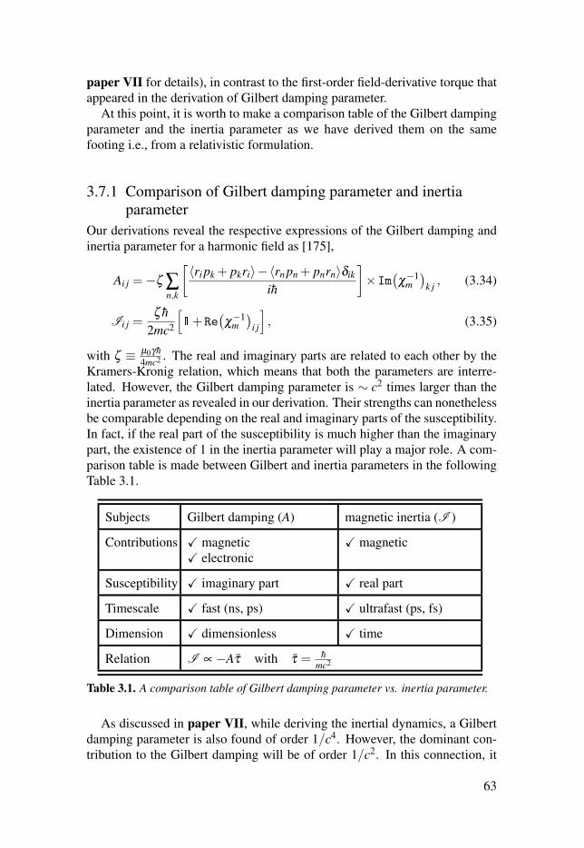
paper VII for details), in contrast to the first-order field-derivative torque thatappeared in the derivation of Gilbert damping parameter.

At this point, it is worth to make a comparison table of the Gilbert dampingparameter and the inertia parameter as we have derived them on the samefooting i.e., from a relativistic formulation.

3.7.1 Comparison of Gilbert damping parameter and inertiaparameter

Our derivations reveal the respective expressions of the Gilbert damping andinertia parameter for a harmonic field as [175],

Ai j =−ζ ∑n,k

[〈ri pk + pkri〉−〈rn pn + pnrn〉δik

ih

]×Im

(χ−1

m)

k j , (3.34)

Ii j =ζ h

2mc2

[�+Re

(χ−1

m)

i j

], (3.35)

with ζ ≡ μ0γ h4mc2 . The real and imaginary parts are related to each other by the

Kramers-Kronig relation, which means that both the parameters are interre-lated. However, the Gilbert damping parameter is ∼ c2 times larger than theinertia parameter as revealed in our derivation. Their strengths can nonethelessbe comparable depending on the real and imaginary parts of the susceptibility.In fact, if the real part of the susceptibility is much higher than the imaginarypart, the existence of 1 in the inertia parameter will play a major role. A com-parison table is made between Gilbert and inertia parameters in the followingTable 3.1.

Subjects Gilbert damping (A) magnetic inertia (I )

Contributions � magnetic� electronic

� magnetic

Susceptibility � imaginary part � real part

Timescale � fast (ns, ps) � ultrafast (ps, fs)

Dimension � dimensionless � time

Relation I ∝−Aτ with τ = hmc2

Table 3.1. A comparison table of Gilbert damping parameter vs. inertia parameter.

As discussed in paper VII, while deriving the inertial dynamics, a Gilbertdamping parameter is also found of order 1/c4. However, the dominant con-tribution to the Gilbert damping will be of order 1/c2. In this connection, it

63

is worth mentioning that the Gilbert damping parameter and inertia parametercan be seen as a series of higher orders of 1/c2. This will be visible if onederives the higher order terms in the FW transformation. The correspondingterms will have higher order time derivatives of electric and magnetic fieldwhich will then follow our derivations.

We note that the Gilbert and inertia parameters that we derive are intrinsicand applicable to a pure and isolated system. There are several other extrin-sic factors that can contribute to these parameters as well. For example, theenvironmental effects, radiation, interactions of spins with other quasiparti-cles (phonons), interfacial effects, spin pumping in magnetic multi-layers canmodify these parameters [161, 176–179].

3.8 Spin currentsSo far, in the discussions, the spin currents have not been considered. Toexplain many dynamical phenomena (e.g., domain wall motion, skyrmion dy-namics etc.) in magnetic systems, one has to incorporate the spin current terms[52]. These spin-polarized currents can induce a local torque on the magne-tization that has been proposed by Slonczewski [43] and Berger [44]. Thiseffect is called spin-transfer torque (STT) which only requires the flow of anelectrical current. This is realized in a multilayer system where the two fer-romagnetic layers are separated by a nonmagnetic layer. The possible effectof STT is pictorially described in Fig. 3.6. To account for the current-induced

Figure 3.6. Schematic diagram for STT. First, an electrical current je enters into a fer-romagnetic layer, the electrons get spin-polarized when they leave the first layer. Thisgenerated spin-polarized current then travels to the next ferromagnetic layer causing atorque to the pre-existing magnetization.

STT, the LLG equation has to be extended and these torques has been writtenas [44, 45, 136]

∂MMM∂ t

=−γ MMM×HHHeff +α MMM× ∂MMM∂ t

−bJ MMM× [MMM× ( jjje ·∇∇∇)MMM]− cJ MMM× ( jjje ·∇∇∇)MMM , (3.36)

64

where the last two terms explain the STT. bJ is termed as adiabatic STT pa-rameter, while cJ defines the nonadiabatic STT. These torques account for theaction of a spin-polarized current on the magnetization gradient.

In the theory of magnetization dynamics, these torques derive from thenonequilibrium spin density (nonequilibrium conduction electrons) which ex-erts a torque on the pre-existing local magnetization [136]. These current in-duced torques can also be derived by using a symmetry considerations [180].However, in our formalism, the corresponding continuity equation of Eq. (3.14)provides deep insight into the torques. Following the discussion of Sec. 3.4.1,one can write down the nonrelativistic magnetization dynamics as

∂MMM∂ t

∣∣∣NR

+1e

[MMM(∇∇∇ · jjjNR

e)+(

jjjNRe ·∇∇∇)MMM

]=−γ0MMM×HHHeff . (3.37)

The nonrelativistic dynamics precisely shows the precession of magnetizationand the effect of nonrelativistic current on the dynamics. Now, as there areno source or sink available in the system, the divergence of the current den-sity must go to zero, implying the second term in the left-hand side of Eq.(3.37) vanishes. The other current term in the left-hand side of Eq. (3.37)takes into account the inhomogeneous magnetization and the correspondingtorque can be written as the current induced adiabatic torque that takes theform ∼ ( jjjNR

e ·∇∇∇)MMM [45, 136, 181, 182]. Therefore, the adiabatic STT can berecovered within the nonrelativistic magnetization dynamics.

However, the relativistic magnetization dynamics shows completely differ-ent dynamical behavior. We have extensively discussed that the Gilbert damp-ing originates from the relativistic spin-orbit coupling. Alongside, there is arelativistic correction to the precession term that is coming from the intrinsicspin-orbit coupling as well. The relativistic magnetization dynamics can bewritten as

∂MMM∂ t

∣∣∣R+

1e

[MMM(∇∇∇ · jjjR

e)+(

jjjRe ·∇∇∇

)MMM]=−γ ′0MMM×HHHeff +MMM×

(A · ∂MMM

∂ t

),

(3.38)

where γ ′0 parameter corresponds to the relativistic precession, Ai j is the Gilbertdamping tensor and jjjR

e is the relativistic current density that has to be derivedfrom the relativistic Hamiltonian. The latter contains the effect of spin-orbitcoupling plus the additional contributions from the relativistic corrections tothe exchange field (see Sec. 2.5.5) as jjjR

e = jjjsoc + jjjother. The current densitydue to the spin-orbit coupling can be written as jjjsoc = κ MMM×EEE tot which de-pends on the magnetization; the parameter κ = −e/(2m2c2gμB). Using thisrelativistic current density one can see that the corresponding conductivity isproportional to the magnetization which is at the heart of the anomalous Halleffect. Moreover, if the electric field is directed in a certain direction, thecurrent points along the plane to that is perpendicular to the direction of the

65

field and magnetization. Therefore, the effect of current density due to spin-orbit coupling will be more significant in the interfaces where the spin-orbitcoupling is strong (see Fig. 3.6). Nonetheless, the effect can also be equallyvisible for a single heavy metal where the spin-orbit coupling is strong and ifit has magnetization inhomogeneity. As discussed in paper VIII, accountingthat the curl of the magnetization is zero (magnetization profile is irrotational),the relativistic magnetization dynamics in Eq. (3.38) results in

∂MMM∂ t

∣∣∣R+

κe

MMM× [(EEE tot ·∇∇∇)MMM] =−γ ′0MMM×HHHeff +MMM×(

A · ∂MMM∂ t

). (3.39)

We have not incorporated the effect of the current density due to other rela-tivistic effects than spin-orbit coupling. We know that, the electric field and thecurrent are proportional to each other through the conductivity tensor, there-fore, the torque (second term) in the left side of Eq. (3.39) can be shown toadopt the form ∼ MMM× [( jjje ·∇∇∇)MMM]. This exactly resembles to the torque ofnonadiabatic STT that has been discussed earlier. Here, the nonadiabaticityparameter comprises the strength of spin-orbit coupling and the conductivitytensor. Now, due to spin-orbit coupling, the spin-flip processes are possible,those spin-flip relaxation times can be accounted through the calculation ofconductivity tensor. Hence, we derive the current-induced STT within thespin continuity equation, while starting from the DKS Hamiltonian.

To summarize, the LLG and extended LLG terms have been derived fromthe fundamental DKS Hamiltonian. Within the magnetization dynamics, theprecession of magnetization comes from the Zeeman-like couplings betweenspins and effective field. The intrinsic spin-orbit coupling also contributes tothe relativistic precession when a spherically symmetric potential is assumed.On the other hand, the Gilbert damping derives from the extrinsic spin-orbitcoupling. The corresponding Gilbert damping parameter has been shown tohave two-fold origin: electronic and magnetic which can be calculated fromfirst principles. More importantly, the damping parameter is a tensorial quan-tity while it has been known previously to be scalar. The damping tensor hasalso been shown to contain an isotropic Heisenberg-like damping, anisotropicIsing-like damping and a chiral DM-like damping. Furthermore, for a systemdriven by nonharmonic fields, an additional torque is generated - field deriva-tive torque. This torque can become important for pulsed shaped externalfields which will exert an instantaneous but huge torque on the magnetizationthat might lead to the switching of magnetization. On the same path, we havederived the optical spin-orbit torque that accounts for the manipulation of spinsusing the angular momentum of light. We have also derived the magnetic in-ertial dynamics within an extended LLG equation and the origin of magneticinertia relates to the higher-order spin-orbit coupling. Finally, deriving thespin-currents in the spin continuity equation, we have derived the origin ofadiabatic and nonadiabatic spin transfer torques within extended LLG equa-tion.

66

4. Relativistic Effects in Ultrafast Magnetism

4.1 IntroductionThe study of magnetization dynamics is an exceedingly vast research areawith the involvement of profound physics as discussed in the previous chap-ter. However, realizing these dynamics in technological devices have beenproven to be challenging. Importantly, the unanswered question remains: howfast can the magnetization be manipulated? For example, it has been shownthat the magnetization reversal by an applied magnetic field pulse occurs ina nondeterministic way if the pulse duration is less than 2 ps [9]. Therefore,the possibility of manipulating the spins in an ultrashort timescale appears un-achievable with the application of a magnetic field pulse. The use of an opticalfield pulse (laser) is another option. The main advantage of the latter is that thecontemporary laser pulses are available in the laboratory with a wide range ofpulse durations, where the pulse width can be as low as up to a few attoseconds[10].

Recent advancements of new techniques using optical laser pulses in pump-probe experiments have made it possible to access the sub-picosecond dynam-ics. In a typical pump-probe set up, an ultrashort laser beam is split into twoseparate beams, among which, one acts as pump (higher intensity) and theother acts as probe (lower intensity). First, the pump pulse is directed towardsthe sample to excite and the probe consequently detects the modification (thathas been caused by the pump) within the sample. The pump stimulates theoptical excitations which are very short-lived, therefore, an ultrashort probepulse is needed to measure the modification of the sample. The pulse dura-tions of the pump and probe are usually kept in about a few tens of fs. Thus,the set up allows one to detect a temporal as well as a spatial resolution of thedynamics, given the fact that the probe pulse is delayed with respect to thepump pulse.

Ultrafast demagnetization was discovered more than two decades ago by E.Beaurepaire and co-workers in such a pump-probe magneto-optical Kerr effect(MOKE) experiment on a nickel (Ni) thin-film of ∼ 20 nm. In particular, asudden loss of magnetization was observed within an ultrashort timescale lessthan a ps after the laser pulse hit the sample. The magnetization response ofNi was measured in pump-probe ultrafast spectroscopy as a function of pump-probe time delay (Δt) as shown in Fig. 4.1 [11].

The above-described effects have been roughly accounted for using the phe-nomenological extension of the so-called two temperature model (electrons

67

Figure 4.1. Ultrafast demagnetization is shown. The black dots represent the experi-mental observations and the smooth line shows the follow up of the experimental datapoints. Taken with permission from Beaurepaire et al., Phys. Rev. Lett. 76, 4250(1996). Copyright c© 1996, The American Physical Society.

and lattice) including the spins. Thus the system has three different reservoirsand they evolve according to three coupled differential equations (taking intoaccount their specific heat and the transfer of energy from one to another).The solution of the equations resembles the experimentally observed electrontemperature evolution within the ultrashort timescale [11].

The experiment was followed by several others leading to a similar trend ofultrafast demagnetization [15, 17, 23, 183–185]. Among the metals, mostlythe transition metals (Fe, Co, Ni) have been extensively studied [18, 186–188]. Other systems like ferrimagnets, antiferromagnets and ferromagneticinsulators have shown much more complicated dynamics [189–192]. Manytheoretical investigations have been made till the date, however, the underlyingmechanisms are not properly understood in the ultrashort timescales as yet. Inthe following, we provide a few of the important proposed mechanisms duringultrafast demagnetization processes.

4.2 Mechanisms of ultrafast demagnetization4.2.1 Direct spin-photon couplingThe prime aspect during ultrafast demagnetization is the transfer of angularmomentum within different available degrees of freedom within a material.It has been predicted that the direct coupling of laser photons with the spinscould lead to the transfer of angular momentum from light to the magnetic

68

moments and thus to the demagnetization [16, 193]. However, the estimationson Ni reveal that the direct photo-quenching can only change the magneticmoments by 10−4 μB per Ni atom [194]. Therefore, this negligible amountof photo-quenching cannot be the reason behind the experimentally observedultrafast demagnetization [195].

4.2.2 Electron-electron interactionThe Coulomb interaction among the electrons might also be another mecha-nism of ultrafast demagnetization as the electron-electron interaction is a veryfast process [23]. Krauß et al. investigated the effect of electron-electroninteraction within Elliott-Yafet (EY) like mechanisms that was originally pro-posed for spin-lattice relaxation [196]. The ultrafast demagnetization is pos-sible in EY theory because the spin-orbit interaction does not conserve spinmomentum and any momentum dependent scattering mechanism transfers themomentum from the spins to another reservoir. It has been found that theelectron-electron EY-type scattering mechanisms are very important in ultra-fast demagnetization [197]. Model calculations have also been performed in-cluding the electron-electron and electron-phonon scatterings within the spin-resolved Boltzmann equation. The study suggests that the electron-electronscattering is required for demagnetization, while the electron-phonon scatter-ing is responsible for remagnetization [198].

4.2.3 Electron-phonon interactionSpin-flip due to EY electron-phonon scattering mechanism has been discussedas the key issue for demagnetization [199, 200]. The main idea is the transferof angular momentum from spins to the lattice. Carva and co-workers have de-veloped an ab initio theory to calculate the effect of spin-flip due to electron-phonon scattering where they have concluded that the effect is too small toexplain the amount of observed demagnetization [24, 25]. However, the ques-tion of angular momentum has not been addressed properly as the calculationswith electron-phonon scattering considers the linearly polarized phonon states(they do not carry angular momentum). This consideration assumes the lat-tice to be a perfect sink of angular momentum. In the following, we provideexplanations of the debate over the angular momentum conservation.

Angular momentum conservationAfter the fs laser pulse hits the ferromagnetic sample, the microscopic mech-anisms of the angular momentum transfer from spins to other degrees of free-dom are important and have often been debated. One way to recognize theconservation of angular momentum is that the magnetic sample is not free inthe space, but it is often mounted on a sample holder which then connects to a

69

table on the floor. Thus, the total system is isotropic as a whole and the angularmomentum is conserved, but not the angular momentum of the sample (partof the total system) [201]. One also has to note that, during demagnetizationthere are emissions of electromagnetic waves which are linearly polarized andthey carry the energy of THz regime [202, 203]. These THz waves are ableto interact with the phonon and they can be re-absorbed in the sample. There-fore the strict conservation of angular momentum during fs demagnetizationis arguable [201].

4.2.4 Superdiffusive spin transportA conceptually different approach than the usual sub-atomic interactions hasbeen employed by Battiato et al., that is called superdiffusion theory. Withinthe superdiffusive spin transport, the majority spins travel faster into the sub-strate as compared to the minority spins leading to the demagnetization in thesample [26, 204]. Experimental measurements have been performed in mag-netic multi-layered system of Au/Ni, where the Au layer was hit by the fslaser pulse generating a non-equilibrium hot electrons. Those hot electronstravel through the Au/Ni interface towards the Ni region and efficiently ex-plain the demagnetization in ferromagnet [187]. Similar experiments revealthe importance of ultrafast spin transfer current that directly indicates that thesuperdiffusive spin-transport as the key mechanism for ultrafast demagnetiza-tion [205–207]. The superdiffusion theory, however, depends critically on thecomposition of the sample [208] and it has not been the dominant effect insingle ferromagnetic thin films on insulator substrates [209].

4.2.5 Spin-orbit coupling and excitationWithin this framework, a full ab initio time-dependent DFT formalism hasbeen used to propose an explanation of the observed ultrafast demagnetiza-tion [210]. The ultrashort laser-induced demagnetization has been proposedas a two step process: (1) the laser excites a fraction of electrons, and (2) thespin-orbit coupling of the remaining localized electrons helps in spin-flip tran-sitions. Thus, the spin-orbit coupling is shown to take a fundamental role. Thelatter has been included in the Pauli Hamiltonian taking into account the vectorpotential from the laser pulse to explain the amount of observed demagnetiza-tion [211]. However, in the calculations a very short pulse has been used witha duration of ∼ 2.2 fs and a very high laser intensity (2-3 orders of magnitudehigher than experiments) has been employed. Moreover, the demagnetizationtime has been found to be very short about ∼ 20 fs in bulk Ni in comparisonto the experimentally observed time [210]. In a recent study, a comparisonis made between bulk and thin films demagnetization using ab initio TDDFT[212].

70

4.2.6 Relativistic spin-flip processesTo understand the effect of relativistic spin-flip processes in ultrafast demag-netization, a single 50 fs duration of laser pulse has been used in a pump-probeultrafast spectroscopy experiment [22]. From the experimental observations,it has been proposed that the laser field couples to magnetism in the ferro-magnetic Ni film efficiently during its propagation [22]. The mechanism isdescribed in the following: the fs laser pulse interacts coherently with thecharges and spins of the magnetic Ni thin film, inducing a demagnetization.This coherent step is followed by the incoherent step due to thermalization ofcharges and spins and their interactions with the lattice. A linear decrease ofcomplex Kerr rotation and ellipticity has been found in Ni, which was sug-gested to have its origin in relativistic quantum electrodynamics involving thespin-orbit coupling, beyond the ionic potential [22].

To verify the above-described processes, we need to use the spin densityfunctional theory with the charge and spin correlations, yet including the ef-fective exchange field terms with lowest order relativistic corrections up to1/c2 that includes the proper description of spin-orbit coupling (which wasmissing in Ref. [22]). In other words, we have to use simply the Hamiltonianin Eq. (2.74) that has been derived throughout the Chapter 2. This will bediscussed in more details in Sec. 4.3.

In connection to the previous discussion, it is worth mentioning that Voneschand Bigot used a similar Hamiltonian, however, they considered a strong statichomogeneous magnetic field, BBBM, which was given by the vector potentialAAAM = 1/2 BBBM×RRR, with RRR as the position of electrons. They also separatelyused an electric field, coming from laser EEEL and the corresponding vector po-tential AAAL [213]. Once again, we emphasize that the consideration of homoge-neous magnetic field to account for the exchange fields cannot be included asa vector potential [122]. Therefore, the minimal coupling can only be used forthe vector potential from laser light as (ppp− eAAAL). In their work, they founda significant contribution in the transition matrix elements of the interactionAAAL ·AAAM, while this interaction does not appear in our formulation derived fromthe DKS theory (see Eq. (2.74) for details).

To summarize, the fundamental processes during the ultrafast demagneti-zation in shorter timescale are still debatable and do not have any accuratedescription [21, 184, 214, 215]. It is mainly because of the fact that at theultrashort timescale, the electrons immediately become non-thermal. There-after, the electrons gets heavily excited in or out of the Fermi sea. In this situa-tion, the description of electron or spin temperatures is not strictly valid as thetemperatures are usually defined for thermalized reservoirs. Moreover, at theultrashort timescale, the classical descriptions become invalid and the quan-tum effects become prominent. Along the same line, the transfer of angularmomentum has been a long standing question during the process of ultrafastdemagnetization.

71

Despite of the debate on underlying mechanisms, one can conclude thatthere is not a single mechanism that could explain the huge magnetizationloss. It is probably the combination of several mechanisms that could explainthe experimental observation. Nonetheless, in the following, we describe theinfluence of relativistic spin-flip effects in the demagnetization processes.

4.3 Relativistic magneto-opticsMOKE is itself a relativistic effect due to its direct relation with the spin-orbitcoupling [216, 217]. To be specific, when MOKE is calculated in ab initioelectronic structure theory, the wave functions correspond to the relativisticHamiltonian that includes the spin-orbit coupling. MOKE spectra have beencalculated for uranium [86, 218] and transition metal compounds [219–223]and these have been found to be fully satisfactory. The Kerr spectra can bedirectly obtained through the diagonal and off-diagonal parts of the opticalconductivity tensor (σαβ ) by the following relation [224]

ΦK(ω) = θK(ω)+ iεK(ω) =−σxy(ω)

σxx(ω)√

1+ 4πiω σxx(ω)

, (4.1)

where θK and εK are the Kerr rotation angle and ellipticity respectively. Notethat the above expression is particularly valid for polar MOKE where the mate-rial magnetization is perpendicular to the reflection surface and parallel to theplane of incidence. These optical conductivity tensors are calculated withinKubo linear response formalism that can be expressed as a current-current ormomentum-momentum response function [224, 225]. To derive the responsefunction, the first order interaction Hamiltonian is taken into account (see Ap-pendix B of paper I). We know that the effect of an intensive laser pulse isconsidered through the vector potential, AAA(rrr, t). Now, within an uniform mag-netic field (see Eq. 2.76) and Coulomb gauge one finds rrr ·AAA = 0. A simpleformulation of its time derivative gives:

ddt

(rrr ·AAA) = 0⇒ drrrdt·AAA = rrr ·EEE

⇒ em

ΠΠΠ ·AAA = errr ·EEE . (4.2)

In this case, we only retain the transverse part of the electric field, EEE = − ∂AAA∂ t

for the choice of Coulomb gauge. The left-hand side in Eq. (4.2) defines the in-teraction Hamiltonian, which is the product of momentum operator ΠΠΠ and thevector potential [226]. Thus, we show that the first-order interaction Hamilto-nian can equally be written as the product of positions of electrons (rrri) and theelectric field acting upon them. This formulation is true for the nonrelativis-tic, semirelativistic or fully relativistic case [123]. The conductivity tensor is

72

thereafter derived from the commutators of current density and the first-orderinteraction Hamiltonian. The conductivity tensor adopts the expression of amomentum-momentum response function (see Appendix B of paper I) as

σαβ (ω) =− ie2

m2hV ∑nn′kkk

[f (εnkkk)− f (εn′kkk)

ωnn′(kkk)Πα

n′n(kkk)Πβnn′(kkk)

ω−ωnn′(kkk)+ i/τ

], (4.3)

with the optical energy hω , Fermi-Dirac distribution functions f (εnkkk) and thedifference between the band energies hωnn′(kkk) = εnkkk−εn′kkk. The involved mo-mentum operator can be taken as ΠΠΠ = ppp for the nonrelativistic case, ΠΠΠ = mcαααfor the fully relativistic case. In our case, we derive the corresponding mo-mentum operator from the Hamiltonian in Eq. (2.74) that involves the non-relativistic momentum operator plus the additional contributions coming fromthe relativistic correction and can be as expressed by

ΠΠΠ = ppp+1

4mc2

[2p2

mppp+ iσσσ × (pppV )+μB

{σσσ · (pppBBBxc)+(ppp ·BBBxc)σσσ

+2BBBxc(σσσ · ppp)+2σσσ(BBBxc · ppp)+ i(ppp×BBBxc)}]

. (4.4)

Within relativistic magneto-optics, one calculates the diagonal and off-diagonalconductivity tensors and the complex MOKE spectra of Kerr rotation and Kerrellipticity [224].

4.3.1 Relativistic spin-flip effects in ultrafast demagnetizationIn this section, we discuss the contribution of relativistic spin-flip effects dur-ing ultrafast demagnetization. We have calculated ab initio the real and imag-inary part of the conductivity tensors (diagonal and off-diagonal components)using the relativistic four component extension of the augmented sphericalwave (ASW) method [227], within local spin density approximation in DFT.To do so, we have solved numerically the DKS Hamiltonian in order to find outthe electron spinor wave function which includes the effect relativistic correc-tions e.g., spin-orbit interaction. The momentum matrix elements have beencalculated using the relativistic wave functions. The momentum operator inEq. (4.4) includes the spin-orbit coupling and thus accounts for the spin-flipeffects because the spin-orbit interaction and other relativistic effects do notconserve the spin angular momentum. To quantitatively account for the spin-flip effects, we calculate the conductivity and complex MOKE spectra of Niand Fe in the following taking into consideration the relativistic and nonrela-tivistic momentum operator. The contributions due to the relativistic spin-flipeffects can be captured by taking their difference.

As described in paper I, the calculations of conductivity spectra and com-plex MOKE overlap with each other while taking the nonrelativistic momen-tum matrix elements in contrast to the relativistic momentum matrix elements

73

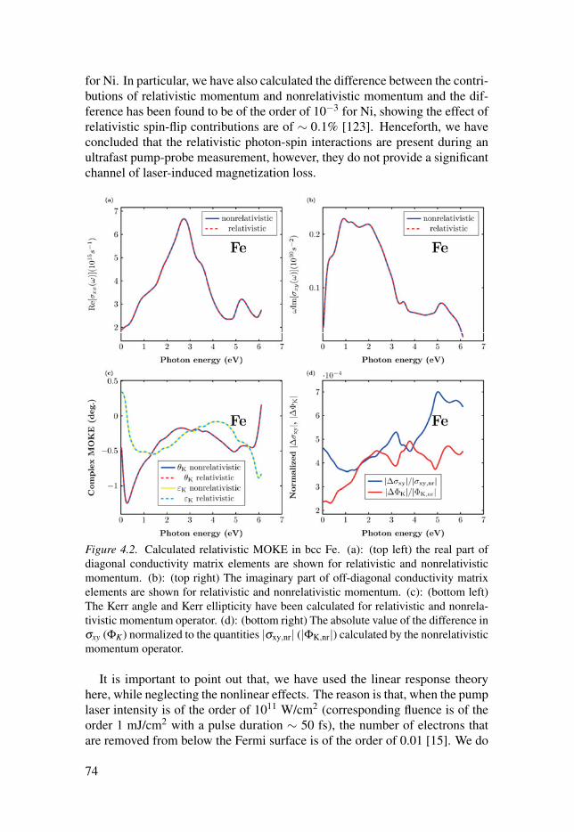
for Ni. In particular, we have also calculated the difference between the contri-butions of relativistic momentum and nonrelativistic momentum and the dif-ference has been found to be of the order of 10−3 for Ni, showing the effect ofrelativistic spin-flip contributions are of ∼ 0.1% [123]. Henceforth, we haveconcluded that the relativistic photon-spin interactions are present during anultrafast pump-probe measurement, however, they do not provide a significantchannel of laser-induced magnetization loss.

Figure 4.2. Calculated relativistic MOKE in bcc Fe. (a): (top left) the real part ofdiagonal conductivity matrix elements are shown for relativistic and nonrelativisticmomentum. (b): (top right) The imaginary part of off-diagonal conductivity matrixelements are shown for relativistic and nonrelativistic momentum. (c): (bottom left)The Kerr angle and Kerr ellipticity have been calculated for relativistic and nonrela-tivistic momentum operator. (d): (bottom right) The absolute value of the difference inσxy (ΦK) normalized to the quantities |σxy,nr| (|ΦK,nr|) calculated by the nonrelativisticmomentum operator.

It is important to point out that, we have used the linear response theoryhere, while neglecting the nonlinear effects. The reason is that, when the pumplaser intensity is of the order of 1011 W/cm2 (corresponding fluence is of theorder 1 mJ/cm2 with a pulse duration ∼ 50 fs), the number of electrons thatare removed from below the Fermi surface is of the order of 0.01 [15]. We do

74

not expect the role of additional many-body effects for such a small numberof electrons in the exited states, thus the normal linear response theory withinDFT will be reasonably enough to capture the experimental evidences. How-ever, we note that for a higher intensity (∼ 1014−1015 W/cm2), alternativelyhigher fluence (intensity per second), one has to consider nonlinear effects,beyond linear response theory [210].

In connection to the magneto-optics in Ni, we furthermore show the calcu-lated relativistic magneto-optical effects for bcc Fe in Fig. 4.2.

We find the similar conclusion for Fe as in the case of fcc Ni. It is seen fromthe plots in Fig. 4.2 that the relativistic and nonrelativistic contributions of mo-mentum matrix elements to the MOKE spectra almost overlap with each other.Additionally, we find that their normalized differences are very small and theorder is 5× 10−4(×1015 s−1) for both the conductivity response and MOKEspectra. Therefore, we conclude that the relativistic photon-spin interactionsare present (and also the relativistic spin-flips) during the magneto-optical phe-nomena, however, their contributions are negligibly small to explain the largeloss of magnetization within ultrashort timescales.

4.4 Coherent ultrafast magnetismThe ultrafast demagnetization is experimentally determined by using a pump-probe spectroscopy technique for the MOKE spectra. In this experiment, themagnetic sample is being exposed to the pump pulse and consequently themagnetization is probed by measuring the Kerr rotation angle of the outgoingprobe pulse. The intensity of the pump pulse is much higher than the probe.The differential Kerr angle in Ni is plotted against the pump-probe time-delay,τ , in the left panel of Fig. 4.3, nicely showing the behavior of ultrafast demag-netization within ∼ 250 fs range. The differential Kerr angle is defined usingthe following relation:

Δθ(τ)θ

=θ pu

pr (τ)−θ prnone

θ prnone

. (4.5)

We mention that θ pupr (τ) is measured as the Kerr rotation angle of the reflected

probe beam, once the pump has hit the sample and the angle is expressed asa function of pump-probe time delay. θ pr

none obviously determines only the re-flected probe Kerr rotation without the pump beam and thus it is not a functionof time-delay.

As shown in Fig. 4.3(a), the MOKE measurements in Ref. [22] have beencarried out with two different configuration set ups of pump and probe: (i) thepump and probe polarizations are parallel to each other i.e., θPP = 0o that hasbeen marked with red solid dots and (ii) the pump and probe polarizations areperpendicular to each other i.e., θPP = 90o that has been marked with blue hol-

75

Figure 4.3. Coherent ultrafast magnetism in Ni. (a) (left panel) The normalized dif-ferential Kerr angle is plotted against the pump-probe delay in fs for two set ups.The red data is for when the pump polarization is parallel to the probe polarizationand the blue corresponds to pump polarization being perpendicular to the probe. (b)(right panel) The difference between the two plots in the left panel is presented, whichclearly shows the coherent pump-probe contribution only. [Reproduced with permis-sion from Bigot et al., Nat. Phys. 5, 515 (2009). Copyright c© 2009, MacmillanPublishers Limited. All rights reserved.]

low dots. One can observe that the two configurations produce the same mea-surements (overlap with each other) in longer timescales showing the ultrafastdemagnetization and remagnetization, however, a non-negligible difference isobserved within first 100 fs. This is more clear from the plot in Fig. 4.3(b),showing the difference between two Kerr rotations, θ pu

pr∣∣PP=0o−θ pu

pr∣∣PP=90o as

a function of time-delay, where a dip within 100 fs is observed. Now it is ob-vious that the latter plot completely depends on the polarization of pump andprobe. This observation is known as the coherent ultrafast magnetism [22].

Already in their work, Bigot et al. [22] proposed the microscopic originto be the relativistic quantum electrodynamics, beyond spin-orbit interactioninvolving ionic potential. To account for the relativistic Hamiltonians, effortshave been made to derive the FW transformation of the Dirac Hamiltonianand finding the higher-order relativistic correction terms, that can be useful todescribe the experimental observation [90]. Under the extreme light-matterconditions, the modification of electron-electron interactions has been studiedwith the Dirac-Breit Hamiltonian and the corresponding FW transformation,where it has been shown that the electric field from the light can coherentlymodify the two electron interactions [228]. There have also been attemptsto classically model the observed coherent ultrafast experiments by using theself-consistent mean-field approximations, which includes the nonlinear ef-fects [229–233]. There, the consideration is to use the nonlinear Drude-Voigtmodel and include the effective magnetic field inside the material, togetherwith up to the third order polarization created by the bound and free charges.The total mean-field is considered as the combination of the static molecular

76

mean field (that exists without the light perturbation) and the light-inducedmean field of Weiss type. The latter includes the spin-orbit interaction of elec-tric field from light with the material spins. However, the set of electric fieldand vector potential are considered within the material as (EEEmat, AAAmat) andfrom the laser as (EEE,AAA) and different possible combination of interactionse.g., EEEmat×AAA, EEE×AAAmat etc. have been treated [233].

It should be noted that, our approach is different as we argue that the ma-terial’s magnetic field is very large (order of 103 Tesla), which comes fromthe exchange field. It has been concluded that the material’s magnetic field isabout 510 Tesla in Ref. [233]. Therefore, it is clear that AAAmat is nothing buta measure of the exchange field. We have already pointed out earlier (in Sec.2.4) that the consideration of vector potential within the material (AAAmat) as aminimal coupling, is not strictly valid for exchange field and the correspond-ing magnetic magnetic field can not be written as BBBmat = ∇∇∇×AAAmat. Instead,we have found in Eq. (2.74), a quadratic interaction term of fields from light,which is recognized as the gauge invariant part of the spin-orbit coupling. Thecorresponding Hamiltonian which we call spin-photon coupling Hamiltonian,is found to have the expression [163, 164]

Hspin−photon =e2h

4m2c2 σσσ · (EEE×AAA) , (4.6)

where the electric field is defined as EEE = −∂AAA/∂ t. Using the plane wavesolutions to the Maxwell’s equations, the corresponding Hamiltonian can bewritten as

Hspin−photon =e2h

8m2c2ωσσσ ·Re

[− i(EEE0×EEE0�)] , (4.7)

where ‘Re’ defines the real part and general elliptically polarized light fieldsare assumed as EEE0 = E0/

√2(eeex +eiηeeey) with the ellipticity parameter η . Now

in a typical pump-probe experimental set up, the above-mentioned electricfields can be due to pump or probe or both. The energies of both the pump andprobe have been accounted to have the same ω in Eq. (4.7), however, the sameexpression is not valid if the photon energies of pump and probe are different.A detailed calculation of the Hamiltonian with different frequencies of pumpand probe has been presented in paper VI. In the following, we discuss theeffect of such a Hamiltonian in explaining the coherent ultrafast magnetismthat has been observed in the experiment.

4.4.1 Induced optomagnetic fieldAs discussed in earlier Sec. 3.6.5, the Hamiltonian in Eq. (4.7) can be under-stood as the coupling of light’s angular momentum to the spin. Therefore,the Hamiltonian provides new insight to optically manipulate the spins. In

77

the same context, considering a Zeeman-like coupling as −gμBσσσ ·BBBopt, theinduced optomagnetic can be expressed as

BBBopt =e2h

8m2c2ωgμBRe[i(EEE0×EEE0�)] . (4.8)

We should note here that the electric fields involved are purely from the laserlight. To explain the origin of coherent ultrafast signals, we argue that duringthe first 100 fs, pump and probe beams interact with each other, given the factthat their pulse duration is of the order of 50 fs. Therefore, we consider all thepossible interactions between pump and probe as described by the followingterms: EEE0

pu×EEE0�pu (pump-pump), EEE0

pr×EEE0�pr (probe-probe), EEE0

pu×EEE0�pr (pump-

probe) and EEE0pr×EEE0�

pu (pump-probe) [164]. It is worth to mention here that,the pump-pump and the probe-probe interactions will only contribute if theyhave nonzero ellipticity, for linearly polarized pump and probe, their contri-bution will become zero. However, the pump-probe interaction will alwayscontribute even for linearly polarized pulses. Considering the linearly polar-ized pump and probe beams, traveling towards z-direction, if the polarizationsof pump and probe are parallel to each other (θPP = 0o); the electric fields canbe taken as, EEE0

pu = (E0pueeex,0) and EEE0

pr = (E0preeex,0). In this case, the induced op-

tomagnetic field will be zero as all the above-mentioned contributions will bezero. On the other hand, if the pump and probe polarizations are perpendicularto each other (θPP = 90o); the electric fields can be taken as, EEE0

pu = (E0pueeex,0)

and EEE0pr = (0,E0

preeey). In this case, the induced optomagnetic field will not bezero as all the pump-probe interaction contributions will be non-zero. In par-ticular, the magnitude of the optomagnetic field that we have derived has theexpression [164]:

Bopt =eh

4mc2

|E0pu||E0

pr|hω

. (4.9)

Therefore, the strength of the optomagnetic field depends on the amplitudesof the pump and probe beams. Considering the experimental values of pumpand probe electric field amplitudes, the optomagnetic field has been found tobe as large as few μT upto mT.

Along with the magnitude, we also mention that the induced optomagneticfield depends on the pump-probe delay; if the delay time is longer, the pumpand probe do not interact with each other and the corresponding optomagneticfield will be zero. A full picture involving different interactions to the inducedoptomagnetic field, is summarized in the following Table 4.1 for linearly po-larized pump and probe beams.

It is important to mention that, in pump-probe experiments, the pump canbe elliptically polarized to capture the effect of light’s helicity. This is em-ployed for helicity dependent investigations e.g., AO-HDS. For example, wecan mention the study of light-induced spin oscillations in DyFeO3 by Kimel

78

Contributions to induced optomagnetic field

Pumpbeam

Probebeam

EEE0pu×EEE0�

pu EEE0pr×EEE0�

pr EEE0pu×EEE0�

pr EEE0pr×EEE0�

pu

(E0pueeex,0) (E0

preeex,0) 0 0 0 0

(0,E0pueeey) (0,E0

preeey) 0 0 0 0

(E0pueeex,0) (0,E0

preeey) 0 0 �= 0 �= 0

(0,E0pueeey) (E0

preeex,0) 0 0 �= 0 �= 0

E0pu(eeex,eeey) E0

pr(eeex,eeey) 0 0 �= 0 �= 0

Table 4.1. All possible configurations of pump and probe for linearly polarized light.

et al. [28], where circularly polarized pump pulses have been used and probedby linear polarized light. As discussed in the last paragraph, the impact ofpump-pump interaction will become important in this case and will have largerimpact on the induced optomagnetic field because of the fact that the intensityof the pump beam is about 103 times higher than that of the probe. Such con-tributions have been listed for possible configurations of elliptically polarizedpump and linear polarized probe in Table 4.2. Considering the experimentalvalues of pump electric field amplitude, the pump-pump interaction producesan optomagnetic field of the order of few mT [164].

For elliptically polarized light, η defines the ellipticity parameter whichtakes the value η = 0 for linear polarization, while η =+π/2 and η =−π/2for right and left circular polarized light, respectively. Needless to say that,when both the pump and probe are elliptically or circularly polarized, all theabove four interactions will become non-zero and thus they all will contributeto the induced optomagnetic field.

Contributions to induced optomagnetic field

Pump beam Probebeam

EEE0pu×EEE0�

pu EEE0pr×EEE0�

pr EEE0pu×EEE0�

pr EEE0pr×EEE0�

pu

E0pu(eeex,eiηeeey) (E0

preeex,0) �= 0 0 �= 0 �= 0

E0pu(eeex,eiηeeey) (0,E0

preeey) �= 0 0 �= 0 �= 0

Table 4.2. All possible configurations of elliptically polarized pump and linearly po-larized probe light.

79

Using the experimental parameters of the pump-probe intensity, wavelength,photon energies, pulse durations, we can estimate the induced optomagneticfield numerically. We have found that the optomagnetic fields are small andrange from the order of few mT to μT depending on the pump and probe in-tensities that have been used in the experiments. Such small fields can not beneglected at all, in fact they can be very much important for thin films. For ex-ample, here we mention that a magnetic field of about 10-20 mT of magneticfield is able to switch the magnetization of a thin film [234].

To summarize, in the first part of this chapter, we have quantitatively stud-ied the effect of relativistic spin-flip processes in laser-induced ultrafast de-magnetization. We have carried out ab initio calculations of optical conduc-tivity and MOKE spectra with relativistic and nonrelativistic momentum ma-trix elements. Due to the spin-orbit coupling and other relativistic effects,the relativistic momentum should capture all the possible relativistic spin-flipprocesses. We have found that the modification of the optical conductivityand MOKE spectra due to the relativistic momentum matrix elements are verysmall (∼ 0.1%) in Ni and Fe. Therefore, we conclude that although the rela-tivistic spin-flip processes do exist during ultrafast demagnetization, they donot provide a notable channel for the huge magnetization loss that has beenobserved in the demagnetization experiments.

In the later part of the chapter, we have explained the origin of coherent ul-trafast magnetism with the help of a novel relativistic Hamiltonian which effi-ciently couples the electron’s spin to the angular momentum of light. The cor-responding Hamiltonian stems from the gauge invariant part of the spin-orbitcoupling. We have rewritten this Hamiltonian in order to explain a Zeeman-like coupling between the electron’s spin and an optically induced magneticfield which is proportional to the ellipticity and the intensity of light. Usingthe relativistic optomagnetic field expression, we have evaluated its strengthduring the interaction of pump and probe within the first 100 fs of the dy-namics. We have found that the optomagnetic field strongly depends on thepolarization of pump and probe; for linearly polarized pump and probe, ifthe polarizations are parallel to each other, the optomagnetic field becomeszero. However, if the polarizations are perpendicular to each other, the in-duced optomagnetic field becomes non-zero and it is directly proportional tothe amplitude of pump, amplitude of probe, however, inversely proportionalto the frequencies of both. For the latter case, the optomagnetic field dependson the pump-probe time delay as well. It is however worth to note that, if thetime delay is large then the interactions between pump and probe cannot beaccounted. Finally, we remark that similar optomagnetic fields can be antici-pated for the elliptically polarized laser pulses.

80

5. Inverse Faraday Effect

5.1 IntroductionThe Faraday effect (FE) is a magneto-optical phenomenon, which describesthe rotation of the plane of polarization of linearly polarized light, while itpasses through a magnetic medium [235]. If the medium does not possess anyintrinsic magnetic moment, the medium should be kept in a magnetic field.In contrast, the inverse Faraday effect (IFE) occurs when circularly polarizedlight propagates through a nonabsorbing or absorbing crystal, where it inducesa magnetic moment [236]. The induced magnetization due to the IFE changessign when the circular polarization is changed from right to left circular polar-ization. Now, as linearly polarized light can be considered as the superpositionof equal amounts of right and left circularly polarized rays, it was thought thatlinearly polarized light cannot induce IFE. However, using the orbital angularmomentum of light, it has been shown that linearly polarized light can inducea magnetization as well [237]. The IFE is observed in paramagnets [238, 239]and plasmas [240–243] with circularly polarized light. In the same context,various models for the IFE have been proposed in the last decades [244–247].However, there are many open questions. For example, it is not properly un-derstood whether the IFE induces a magnetic field or a magnetization withina material.

Here, we describe the IFE in a way that it induces a magnetic moment(magnetization), ΔMMM which is proportional to the cross product of electricfields, ∼ EEE×EEE� i.e., the intensity of the incident light. This induced magneti-zation behaves differently for nonmagnetic systems and for magnetic systemsas illustrated in Fig. 5.1. The induced magnetization can exert a torque onthe preexisting magnetization and thus can assist to the magnetization switch-ing in a magnetic material [248]. Therefore, the IFE has been instrumentalto achieve all-optical switching in the ultrafast regime [28, 29]. This showsthat the microscopic understanding of the IFE is potentially very rich. In thefollowing, we describe the classical theory of the IFE followed by its quantumdescription, however, including the effect of light absorption.

5.2 Classical descriptionThe classical description of the IFE starts with the assumption of a free elec-tron gas, neglecting their quantum effects [249]. In the free electron model,

81

Figure 5.1. A schematic view of the inverse Faraday effect. (Left) For nonmag-netic and antiferromagnetic systems, where the net magnetization is zero, the oppositelight’s helicity induce same but opposite magnetizations (ΔMMM). (Right) For magneticsystems, where there is a net magnetization, MMM present, the opposite light’s helicityinduce asymmetric magnetizations.

the collisions of the electrons with the other electrons and ions are neglected.Moreover, in the absence of any external electromagnetic field, the electronsmove freely on a straight line unless they collide with the others. While mov-ing inside the metal, the electrons can collide with each other. These collisionsare instantaneous and as a consequence, the electrons abruptly change theirvelocity and momentum. The probability of an electron having a collisionwithin a time interval dt is γdt and that does not depend on the position of theelectrons (γ is the collision rate, which takes into account the absorption oflight). The electrons are assumed to have achieved thermal equilibrium withthe surroundings after the collisions. With these assumptions, and accordingto Newton’s second law, the dynamics of the electrons can be modeled by theDrude-Lorentz theory [245, 250]

md2rrr(t)

dt2 +mγdrrr(t)

dt+mω2

0 rrr(t) = FFF(t) . (5.1)

rrr(t) denotes the instantaneous position of the electron and the electromagneticforce FFF(t) = eEEE, acting on the electron. γ accounts for energy loss processesi.e., dissipations (γ = 0 for the nonabsorbing materials) and ω0 is the angularfrequency of the electron, which represents the electrons are bound by poten-tial ω2

0 rrr(t). To obtain the IFE induced effects, the electric field is taken as cir-cular polarization EEE = E0 (sinωt eeex + cosωt eeey), with ω , the frequency of theincident light while the light is propagating towards the z-direction. The nextstep is to solve Eq. (5.1) for the position, rrr(t) and the velocity vvv(t) = drrr(t)

dt .Now, we know that for a classical magnetization in materials, the magneticmoment is proportional to the function rrr× jjj, where jjj = nevvv defines the cur-

82

rent density [251]. The induced orbital magnetization is then computed asrrr(t)× drrr(t)

dt [250]. For the asymptotic solution the induced magnetization canbe explicitly calculated and will be given as

MMMIFE =−Ne3

2m2ω

(ω2−ω20 )

2 + γ2ω2 E20 eeez , (5.2)

where N is the electron density. Note that the magnetization is induced in thesame direction of the light’s propagation. We notice that the induced mag-netization is proportional to the intensity (square of the amplitude of electricfield) of the light, as originally proposed by Pitaevskii [236]. However, theeffect of absorption was not considered in the thermodynamic description byPitaevskii. Therefore, the consideration of the parameter γ underlines the maindifference between the above-given classical Drude-Lorentz description andthe approach of Pitaevskii [250]. This is realized by the following relationbetween the parameters ruling FE (νFE) and IFE (νIFE) [250, 252]:

νIFE−νFE

νIFE +νFE=− iγω

ω2−ω20. (5.3)

These parameters are called Verdet constants for FE and IFE. As the deriva-tion by Pitaevskii [236] was based on the dissipationless media (γ = 0), theequivalence of two parameters ruling FE and IFE was concluded. In the clas-sical theory, however, only if one considers γ = 0, this equivalence is realized.The classical treatment thus provides a first step to understand the IFE whileit accounts for the light’s absorption. However, for realistic and more materialspecific calculations of the IFE, the quantum effects have to be included.

In the following, we present the quantum theory of the IFE and the imple-mentation of the theory to calculate the IFE induced parameters.

5.3 Quantum descriptionThe microscopic theory of IFE was described in the context of the possibilityof achieving ultrafast optical control of magnetism [253]. The proposal wasthat IFE is an effect stemming from a Raman-like coherent scattering mecha-nism which generates an ultrafast and efficient magnetic field. When the laserpulse hits the sample, an electron is excited to a higher quantum state. Thisleads to the transition of the electron back to an another quantum state. How-ever, if the transition is driven by an electric dipole, the spin state cannot bechanged because within the electric dipole approximation spin does not in-teract with the electromagnetic field of the laser light. On the other hand, amagnetic dipole transition allows the spin-flip due to the interaction betweenthe electron spin and the magnetic field. Therefore, first the electric dipole

83

transition followed by a magnetic transition would leave the electron in a fi-nal magnetic state that is different than the initial one. The whole process isschematically described in Fig. 5.2.

Figure 5.2. The Λ-like transitions for three level system. The laser light causes thetransition from initial state, |i〉 to a intermediate state | j〉 and then finally back to thefinal state | f 〉 which has different magnetic state from the one in initial. Adapted withpermission from Hansteen et al., Phys. Rev. B 73, 014421 (2006). Copyright c© 2006,The American Physical Society.

First, an optical excitation of hω1 initiates the transition of an electron froman initial to a higher virtual state (intermediate), with a large spin-orbit cou-pling. As the spin is not conserved, the spin-flip becomes allowed. Radiationat the energy hω2 then stimulates the relaxation of the electron back to thefinal ground state. Note that, due to a spin-flip in the intermediate state, theelectron will be in a different magnetic state. During the final transition a radi-ation of h(ω1−Ωm) energy will be released and a magnon of energy hΩm willbe created to compensate the energy. To account for the Raman-like processesand population of the different states during the IFE, an effective Hamiltonianapproach has been considered, including the electron-electron interactions andspin-orbit coupling [246, 254].

In a further study by Battiato, Barbalinardo and co-workers [204, 250, 252],they employed the second order density response of the states to the circularlypolarized light. In their work, the quantum Liouville-von Neumann equationwas solved along with the perturbation from the circularly polarized light. Theperturbation was treated as the interaction Hamiltonian V (t) = e∑i rrri · EEE =em ∑i pppi ·AAA, where rrr and ppp are the electron position and momentum operatorsrespectively, EEE and AAA define the time-varying electric field and correspondingvector potential from the light. As discussed in Ref. [204], the static part ofthe second order density matrix response, ρ [2], has been shown to contributeto the inverse Faraday effect. The induced magnetization is calculated as thecontributions from the orbital and the spin angular momentum and they are

84

evaluated as

MMMIFE = μBTr[(LLL+gSSS)ρ [2]] , (5.4)

where LLL and SSS denote the orbital and spin angular momentum operators re-spectively. The static part of the second order response has three terms andtheir complex conjugates. This means that the optically induced magnetiza-tion has three contributions which can be written as

MIFE = (Ko +KdA +KdB + c.c.)E20 , (5.5)

with E0 the amplitude of the light’s electric field. These three contributions canbe expressed in terms of the momentum and magnetization matrix elements asfollows [255]

Ko =e2

m2ω2 ∑n�=m;l

Mmn

p+nl p−lm( fm− fl)El−Em+ihΓlm−hω −

p−nl p+lm( fl− fn)En−El+ihΓnl−hω

En−Em + ihΓnm,

KdA =e2

m2ω2 ∑n,l

Mnn

(p+nl p−ln( fl− fn)

(El−En + ihΓln− hω)2 −p−nl p+ln( fn− fl)

(En−El + ihΓnl− hω)2

),

KdB =e2

m2ω2 ∑n,l

Mnn

hωp+nl p+ln( fn− fl)(ihΓln− hω)

(El−En)2 +(hΓln + ihω)2 . (5.6)

Here, pnl are the matrix elements of the momentum operator. These are calcu-lated with the relativistic electronic states |nkkk〉 corresponding to the energiesEnkkk. For shake of brevity the momentum kkk has been suppressed in Eq. (5.6).fn = f (Enkkk) are the Fermi-Dirac distribution functions. To account for theright and left circular polarization of the light, we have introduced the raisingand lowering momentum operator as ppp± = ( pppx± ipppy), remembering the factthat the light propagates towards the z-direction. The laser photon energy ishω , and the line-widths are taken into account through Γnl matrix elementsand those are taken as positive parameters, usually chosen to be state indepen-dent.

The above-mentioned expressions of the laser-induced magnetization con-tributions seems mathematically complicated, however, their physical mean-ings are immediately explained. The first term, Ko, arises from the off-diagonal components in the second order perturbed density matrix. Therefore,it includes all the possible optical transitions among different states - electronicRaman-like scattering. First the circular laser light is absorbed by the systemunder study, bringing the system into a virtual excited state. At this stage, theexcited state can couple to the other available electronic or vibrational states ofthe system and therefore finally the system reaches to a state that is differentfrom the initial one. These transitions involve the absorption and the emis-sion of light but not by the equal amount. The second and third terms, KdA

85

and KdB, arise from the diagonal components in the second order perturbeddensity matrix - electronic Rayleigh-like scattering. In these cases, upon theabsorption of light, the system reaches to an excited state. But at this stage,the excited states do not couple to the other available states of the system andconsequently, the initial and final states are the same. These transitions, thus,involve the absorption and emission of light by same amount.

Notice that, in particular, all the terms in Eq. (5.6) diverge when ω → 0 be-cause of its appearance in the the denominator. Hence, it is expected that theinduced magnetization may also diverge at ω → 0. To understand this unusualresult, it is important to keep in mind that the treated field is that inside thematerial. For metals, the reflectivity approaches 100% when ω → 0, implyingthat the field in the material is strongly reduced. While the laser-induced mag-netization is calculated, eventually it induces a corresponding optomagneticfield that can be obtained from the susceptibility of the material as HHH = MMM/χ .We note that, this approach would be valid if both induced spin and orbitalmagnetizations behave in the same way, that is, behave as a response to anapplied Zeeman field.

5.3.1 Ab initio calculationsWe have implemented these contributions to the induced magnetization in anab initio relativistic DFT framework. The effect of absorption which was ig-nored in previous theories [236, 256], is included in our calculation. The im-portant point here that we address is that, there are contributions from theorbital and the spin parts to the induced magnetization. Our configuration setup is such that the laser light travels towards the z-direction, thus for circularlypolarized light the electric field components will be in the x- and y-directions.This means that the induced magnetization will only have the z-component.Therefore, following the definition of laser-imparted magnetization in Eq.(5.4), we get

MzIFE = μBTr

[Lzρ [2]

]+2μBTr

[Szρ [2]

],

=[KL

IFE(ω)+KSIFE(ω)

] Ic. (5.7)

The laser intensity is denoted by I = cε0E20/2 and the frequency dependent

orbital and spin IFE parameters are KLIFE(ω) and KS

IFE(ω) (see paper V fordetails). In this way, the parameters KIFE(ω) have the dimension of inverseTesla.

In practice, when the circularly polarized light hits on a magnetic or non-magnetic system, depending on their magnetic ordering, the absorption ofthe light and all the possible excitations (transitions) happen differently forright and left circularly polarized light. Therefore, it is not possible to predict

86

clearly the behavior of the light-induced magnetizations for two circular polar-izations, unless they are calculated ab initio. In the following, we present abinitio calculations of the IFE which consist of the contributions of the orbital,spin and total induced magnetization in a photon energy span of 0 - 4 eV.

♣ Detail of the calculations

In particular, we calculate the given three expressions in Eq. (5.6) starting fromab initio calculations. To calculate those, we need informations of the severalparameters involved in the expressions. The momentum matrix elements (pnl)are calculated with the relativistic electronic states which are the solutionsof the DKS equation, solving the electron spinor equations for the large andsmall components numerically. The corresponding relativistic band energiesare given by En. The magnetization matrix elements are also calculated simi-larly with the relativistic electronic states. The calculations are performed withthe Fermi-Dirac distributions ( fl) taken as a heavy-side step functions becausethe current calculations do not account for temperature effects. The parameterfor the consideration of broadening or line width is taken as, hΓ = 0.03 Ry.This value has been known to give a very good description of ab initio calcu-lations of linear-order optical response of metals [224]. The polarization of theelectric field is considered for the right circularly polarized light (we denote itas σ+) as EEE = E0 (sinωt eeex + cosωt eeey). Such polarization for a ray, the wavepropagating along −z-direction corresponds to a left circular polarization (wedenote it as σ−). In general, the space and time dependent electric field hasthe following form

EEE(rrr, t) = E0 Re[i|Ψm〉ei(kz−ωt)

]. (5.8)

Here |Ψm〉 are the vectors in the x− y plane. For the right and left circularpolarization, we define those vectors as

|ΨR〉= 1√2

⎛⎝ 1

−i

⎞⎠=

1√2(eeex− ieeey) ,

|ΨL〉= 1√2

⎛⎝ 1

i

⎞⎠=

1√2(eeex + ieeey) . (5.9)

The momentum matrix elements of the contributions in Eq. (5.6) are calculatedwithin the augmented spherical wave (ASW) method with the relativistic bandenergies and wave functions. The calculations of momentum matrix elementsuse the Bessel and Hankel functions as nicely described in the Ref. [220].

♣ Results

The calculated induced magnetization is shown for σ+ and σ− and separatelyfor the contributions from orbital, spin and total magnetization.

87

Nonmagnetic metals:

-0.06

-0.03

0

0.03

0.06

σ+ (Cu)

σ- (Cu)

σ+ (Au)

σ- (Au)

0 1 2 3

-0.06

-0.03

0

0.03

0.06

KIF

E [

1/T

]

σ+ (Pt)

σ- (Pt)

0 1 2 3

Photon energy [eV]

σ+ (Pd)

σ- (Pd)

0 1 2 3 4

Cu, Au

Total Orbital Spin(x10)

Pd, Pt

Figure 5.3. Calculated different contributions to the IFE for nonmagnetic metals asa function of photon energy. (Top panels): The orbital, spin and total IFE effects areshown for Au (black and yellow dashed lines) and Cu (red and blue solid lines). (Bot-tom panels): The orbital, spin and total IFE effects are shown for Pd (black and yellowdashed lines) and Pt (red and blue solid lines). Adapted with permission from Berrittaet al., Phys. Rev. Lett. 117, 137203 (2016). Copyright c© 2016, The AmericanPhysical Society.

In Fig. 5.3, we show the IFE induced magnetization for nonmagnetic met-als (net magnetization is zero) in Cu, Au, Pd and Pt. The calculations showthe existence of finite contributions to not only the spin IFE, but also the or-bital IFE. Note that, the orbital IFE was unknown previously and also wasignored in the original work by Pitaevskii [236]. In addition, we note that themagnitude of the orbital IFE is 10 times larger than the spin IFE. However,these contributions are in the opposite directions for a particular helicity, andtherefore they compete with each other to the total IFE.

The IFE contributions are visibly materials specific. We notice that the in-duced magnetization is larger in Au than the one in Cu in both cases of orbitaland spin IFE. A similar behavior can also be concluded for the case of Pt andPd, where the induced magnetization in Pt is much higher than Pd. All to-gether, the total induced magnetization in Pd and Pt is larger than the one inCu and Au. We can anticipate the fact that the IFE induced magnetizationdiverges at ω → 0 as there are 1/ω2 in the prefactor of the set of Eqs. (5.6).More importantly, the IFE induced effects are antisymmetric in the light’s he-licity which means right circularly polarized light induces exactly the sameand opposite orbital (spin) IFE as left circular polarized light [255].

Ferromagnetic metals: Notably, the ferromagnetic metals show a completelydifferent behavior for the induced IFE than the nonmagnetic metals. The cal-

88

culated induced magnetizations are shown for the 3d transition metals, namely,bcc Fe, hcp Co and fcc Ni in Fig. 5.4.

-0.01

-0.005

0

0.005

0.01

σ+

σ-

-0.02

-0.01

0

0.01

0.02

KIF

E [

1/T

]

0 1 2 3

-0.04

-0.02

0

0.02

0.04

0 1 2 3

Photon energy [eV]0 1 2 3 4

Total Orbital Spin

Fe

Co

Ni

Figure 5.4. Calculated different contributions to the IFE for ferromagnetic metals.The red dashed and blue solid lines show the contributions induced by left and rightcircularly polarized light respectively. (Top panels): The orbital, spin and total IFEeffects are shown for bcc Fe. (Middle panels): the orbital, spin and total IFE effectsare shown for hcp Co. (Bottom panels): The orbital, spin and total IFE effects areshown for fcc Ni. Adapted with permission from Berritta et al., Phys. Rev. Lett. 117,137203 (2016). Copyright c© 2016, The American Physical Society.

In the following, we analyze the obtained results for each material [255].Bcc Fe: The contribution to the spin IFE does not depend on the helicity

of the light, for right and left circularly polarized light, the spin IFE curvesfall on top of each other. However, the orbital IFE depends on the helicity ofthe circularly polarized light. The right and left circular polarization inducean orbital magnetization in the same direction, except in a span of photonenergies 2 - 4 eV. Therefore, the induced total magnetization also points in thesame direction for both helicities. Unlike the nonmagnetic metals, the spinand orbital IFE have the similar order of magnitude and they contribute to thetotal IFE.

Hcp Co: The behavior of induced spin IFE is the same as for bcc Fe, theyalmost overlap with each other for opposite light helicities. The orbital IFEshows a different scenario than bcc Fe. Except for the low energies, the rightcircularly polarized light induces orbital IFE in the opposite direction of thatinduced by the left circularly polarized light and they are asymmetric in thelight’s helicity. Unlike bcc Fe, the right circularly polarized light induces or-bital and spin IFE in the opposite direction, hence, the total induced magneti-zation is less. On the other hand, the left circular polarized light induces spin

89

and orbital IFE in the same direction, increasing the total induced magnetiza-tion.

Fcc Ni: The effect of spin IFE is effectively the same as Fe or Co. However,the orbital IFE are approximately antisymmetric in the light helicity. As seenin hcp Co, a similar behavior of spin and orbital IFE for the right and left cir-cularly polarized light are anticipated. A reason of the asymmetric behavior isthat, for ferromagnets where the net magnetization is nonzero, the time rever-sal symmetry is notably broken already and thus a full antisymmetric behavioris not expected.

Antiferromagnetic materials:

-0.01

-0.005

0

0.005

0.01

σ+

σ-

0 1 2 3

-0.004

-0.002

0

0.002

0.004

KIF

E [

1/T

]

0 1 2 3

Photon energy [eV]0 1 2 3 4

Total Orbital Spin

Fe (AFM)

Fe (no SOC)

x10

Figure 5.5. Calculated different contributions to the IFE for antiferromagnetic Feand ferromagnetic Fe without spin-orbit coupling. The red dashed and blue solid linesshow the contributions induced by left and right circularly polarized light respectively.(Top panel): The orbital, spin and total IFE effects are shown for synthetic antiferro-magnetic Fe. (Bottom panel): The orbital, spin and total IFE effects are shown for bccFe computed without spin-orbit coupling. Adapted with permission from Berritta etal., Phys. Rev. Lett. 117, 137203 (2016). Copyright c© 2016, The American PhysicalSociety.

For antiferromagnetic materials, the net magnetization is zero and onceagain the IFE is expected to have antisymmetric nature with respect to thelight’s helicity. The calculations are presented in Fig. 5.5, for synthetic anti-ferromagnetic Fe. Note that, the spin IFE is about 10 times smaller than theorbital IFE, as was also concluded in the nonmagnetic case. Similar to thenonmagnetic materials, the orbital and spin IFE is induced in opposite direc-tion for a particular helicity. Thereby, the total induced magnetization is alsoantisymmetric in the light’s helicity. In addition, antiferromagnetic Fe shows

90

an photon energy dependence that is different from that of ferromagnetic Fe[255].

To summarize, the ab initio calculations reveal that the IFE is more complexat the fundamental level than it was thought. It is found that the induced mag-netization is antisymmetric in the helicity for the magnetic system with zeronet magnetization. The same is expected for paramagnetic materials as well.However, for ferromagnetic and ferrimagnetic systems, where a net magne-tization exists, the induced magnetization is shown to be asymmetric in thehelicity of the light. Furthermore, in Fig. 5.5, the calculated IFE effects areshown without spin-orbit coupling for ferromagnetic Fe. We see that the with-out spin-orbit coupling, the spin IFE is zero irrespective of the photon energyof the light. This reveals that the spin-orbit coupling is purely responsible forthe laser-imparted magnetization in the spin components.

5.4 Angular magneto-electric couplingThere exist mainly four classes of ferroic orders in a multi-ferroic material.These are: ferroelastic, ferroelectric, ferromagnetic and ferrotoroidic orders.These can be classified in terms of the space inversion and time reversal sym-metry considerations [257]. For example, the space inversion and the timereversal symmetry is conserved for the case of ferroelastic materials becauseonly mechanical processes (stress, strain) are involved. On the other hand, fer-roelectric materials are electrically polarizable means they have spontaneouselectric polarization which comes from the charge density. Now, as the chargedensity depends on the spatial coordinates, the space inversion symmetry isbroken for ferroelectric materials, however, the time reversal symmetry is con-served. The opposite picture is realized for ferromagnetic materials. In thiscase, the the magnetism arises due to the current density which changes signunder the time reversal, however, stays invariant under space inversion. Boththe symmetries are broken for the ferrotoroidic materials, where the alignmentof the magnetic vortices gives rise to a toroidal moment. The observation offerrotoroidic order has been reported recently [258]. These different ferroicorders are pictorially classified in Fig. 5.6.

In this part of the chapter, we are mostly interested in the ferrotoroidic sys-tems and the eventual manipulation of the toroidal moments using electric andmagnetic fields. In the multipole expansion of the magnetic vector potential,the toroidal dipole moment arises from the second order term in the expansion[257]. The toroidal moment can be seen as the cross product between positionand magnetization, MMM. According to the definition, the toroidal moment hasthe following expression [257]

TTT =12

∫rrr×MMM d3r . (5.10)

91

Figure 5.6. The classification of the various ferroic orders according to space and timesymmetry considerations.

In a toroid, the current flowing perpendicular to the toroid creates the moment(see bottom-right part of Fig. 5.6). These current loops will be shifted bythe application of a magnetic field, inducing a polarization - a magnetoelectriccoupling [258]. This manipulation of the toroidal dipole moment is potentiallyimportant for technological purposes e.g., in data storage [257, 259]. Themanipulation has been studied by using a static inhomogeneous field [260],however, the crossed electric and magnetic fields (EEE ×HHH) can also be used[63]. The reason is that the crossed electric and magnetic field breaks both thetime reversal and space inversion symmetry. Therefore, both fields are neededfor manipulation of the toroidal moment. The coupling between the toroidalmoment and the crossed electric and magnetic fields leads to the introductionof a physical energy [62]

E =−12

∫ξ [rrr× (EEE×HHH)] ·MMM d3r . (5.11)

The electric and magnetic fields are considered as EEE and HHH and ξ is the mate-rial dependent strength of the coupling parameter which is unknown. Noticethat, rrr× (EEE×HHH) exactly measures the total angular momentum density of anEM field. Therefore, essentially, the above energy describes the coupling ofangular momentum of an EM field with the electron spin, however, is only putforward from a phenomenological basis and simple symmetry considerations.Nonetheless, the energy can be useful in describing many complex phenom-ena e.g., the anomalous Hall effect [64], spin current model in multiferroics[62], the planar Hall effect and anisotropic magnetoresistance [65].

As of now, the physical energy in Eq. (5.11) is very useful, however, itis phenomenologically described. On the other hand, the energy expressionvaguely resembles to the one of well-known spin-orbit coupling, but with onlythe difference that the angular momentum of light (∝ rrr× (EEE×HHH)) couples to

92

the spin. This energy has been called angular magneto-electric (AME) cou-pling energy [62].

Here, in the below we provide the microscopic derivation of the AME en-ergy in the optical regime while starting from the relativistic DKS Hamilto-nian.

5.4.1 Microscopic derivationIn paper II and paper III, we rigorously derive the physical energy of Eq.(5.11) from the gauge invariant part of the spin-orbit interaction in Eq. (2.82).Thus, we name the corresponding Hamiltonian as the spin-photon couplingthat has the expression [163]

Hspin−photon =e2h

4m2c2 σσσ · (EEE×AAA) (5.12)

Note that, here in contrast to the AME consideration in Eq. (5.11) with staticapplied fields, we consider general time-dependent photon fields. As alreadydiscussed in Chapter 2, there are two electric fields present, the internal andexternal. Therefore, the spin-photon coupling Hamiltonian can be split in anintrinsic part, caused by the microscopic field generated by the crystal poten-tial (EEE int =−1

e ∇∇∇V ), and an extrinsic part that is linked to the external electricfield (EEEext =−∂AAA/∂ t) such that EEE = EEE int +EEEext. Now, within a material, theinternal electric field will be changed by the perturbation from the externalfield. Within the linear response framework, we write

EEE int = EEE0int + γ ·EEEext , (5.13)

with EEE0int, the internal electric field which exists even without applying any

field and γ is a material linear response to the applied field. The parameter γis usually a tensor, however, for a cubic system can be considered as a scalarquantity. With this simplification, the Hamiltonian in Eq. (5.12) can be ex-pressed in two terms:

Hspin−photon =e2h

4m2c2 σσσ · (EEE0int×AAA)+

e2h(1+ γ)4m2c2 σσσ · (EEEext×AAA) . (5.14)

The first term, here, can be dropped because the microscopic field does notexist in the bulk of a solid when it is averaged over an unit cell. Therefore, weproceed while taking the second term into account.

We point out that, the derivation of the Eq. (5.11) from the second term ofEq. (5.14) is based on several strong assumptions. First, the magnetic field isassumed to be uniform that is taken into account through the choice of gauge asAAA = BBB×rrr/2. This is because we assume that the skin depth of the applied EMfield is much larger than the thickness of the system being studied. Second,

93

the results are derived within the Coulomb gauge that means ∇∇∇ · AAA = 0, inaccordance with the Maxwell equations. With the choice of gauge, we insertthe vector potential in second term of Eq. (5.14) and taking its expectationvalue results in

EAME =ξ2

∫MMM · [EEEext× (BBB× rrr)] drrr , (5.15)

where ξ is a material dependent parameter which can be realized due to thefact that ξ ∝ (1+ γ). Third, we have used a linear proportional relationshipbetween the magnetization and magnetic field. As we stressed in Chapter 3,this is typically not true in ferromagnets, where only a small component ofthe magnetization, the induced magnetization, is proportional to the appliedmagnetic field, in contrast to the spontaneous magnetization existing even atzero field. Nonetheless, we expand the expression in Eq. (5.15) and use theproportionality relationship in the second term of the expansion to interchangeBBB and MMM so that we get [163]

EAME =ξ2

∫ [(MMM ·BBB)(rrr ·EEEext)− (MMM ·EEEext)(BBB · rrr)

]drrr

=−ξ2

∫MMM · [rrr× (EEEext×BBB)] drrr . (5.16)

Noticeably, this is exactly the physical energy of the phenomenologically pro-posed AME coupling (see Eq. (5.11)) [62]. We thus provide the microscopicderivation of manipulation of magnetization by the angular momentum oflight; it straightforwardly derives from the DKS Hamiltonian, in particular,from the gauge invariant part of the spin-orbit coupling - the spin-photon cou-pling.

As there are assumptions involved in the derived AME energy in Eq. (5.16),this expression is not general. Instead, we use, in the following, the generalspin-photon coupling Hamiltonian of Eq. (5.12) and discuss how it derives therelativistic correction to the IFE.

5.5 Relativistic contributions to the inverse Faradayeffect

In the discussions of earlier sections (Sec. 5.3), the IFE has been attributedto the second order density response to the circularly polarized light. Theinteraction Hamiltonian of light and electrons that derives IFE is taken as non-relativistic as ppp ·AAA. In this way, the IFE induces a magnetization in a material.On a different note, the essence of IFE was thought to reside on the inducedoptomagnetic field [28, 30, 261]. The latter defines the IFE in a magnetic ma-terial as an effective Zeeman field - optomagnetic field as BBBopt ·MMMi, acting on

94

the atomic spin moment MMMi with conserved length (see the discussion of op-tomagnetic field in the Sec. 4.4.1). As the IFE is a quadratic response of theapplied electric field, the corresponding Hamiltonian has the following form[30]

HIFE = ζ Re[i(EEE×EEE�)

] ·σσσ , (5.17)

where ζ is a material dependent parameter. If the electric fields are taken asthe plane wave solutions of the Maxwell equations i.e., EEE = EEE0ei(kkk·rrr−ωt), onlythe amplitude of the electric field contributes to the IFE induced optomagneticfield. Comparing with the Zeeman field, the optomagnetic field (BBBopt) will beproportional to the real part of the crossed electric field amplitudes such thatthe Eq. (5.17) can be written in the form: HIFE =− ζ

gμBBBBopt ·σσσ .

Here, in the following, we show that the spin-photon coupling Hamiltoniannaturally derives the relativistic optomagnetic field of IFE. We use the trans-verse part of the electric field EEE =−∂AAA/∂ t, such that the vector potential canbe calculated with

AAA =−Re[

iω

EEE0ei(kkk·rrr−ωt)]. (5.18)

Using these considerations, the second term of the spin-photon coupling Hamil-tonian in Eq. (5.14) takes the form

Hspin−photon =−e2h(1+ γ)4m2c2ω

σσσ ·Re [i(EEE0×EEE�0)] . (5.19)

The derived Hamiltonian thus provides precisely the energy related to the IFE(see Eq. 5.17). Considering that the IFE induces a relativistic optomagneticfield, the latter will be given by [163]

BBBopt =e2h(1+ γ)

4m2c2ωgμBRe [i(EEE0×EEE�

0)] . (5.20)

We see that the relativistic optomagnetic field is material dependent and strong-ly depends (inversely proportional) on the angular frequency of the incidentlight, however, linearly proportional to the intensity of the light. Note that,a similar optomagnetic field has been used to describe the coherent ultra-fast magnetism in pump-probe spectroscopy in ultrashort timescales (see Sec.4.4.1). In particular, if we consider an elliptically polarized light of amplitudeE0 and ellipticity parameter η so that

EEE0 =E0√

2

(eeex + eiηeeey

), (5.21)

the magnitude of the induced optomagnetic field in Eq. (5.20) takes the simplerform in terms of the intensity of light I = cε0E2

0/2 and ellipticity as

Bopt =e2h(1+ γ)

4m2c3ε0ωgμBsinη I . (5.22)

95

Again, we point out that as the incoming light has the electric field compo-nents in the x- and y-directions, the optomagnetic field will be induced in thez-direction. This way, the induced field is zero for linearly polarized wave be-cause η = 0 or π leads to sinη = 0. For circularly polarized light (η =±π/2),the induced optomagnetic field is maximal (sinη =±1). The magnitude of theinduced field is equal but opposite for the case of right (η = +π/2) and left(η =−π/2) circularly polarized light, for the same intensity and same angularfrequency. Now, the linearly polarized light is a combination of equal amountsof right and left circularly polarized light and thus the effective induced fieldwill be zero for the linear polarization.

In order to estimate the strength of the induced relativistic optomagneticfields, we use the experimentally used values of the intensity and wavelengthof the contemporary laser source which are largely available. We considercircularly polarized light of intensity I = 10 GW/cm2 and wavelength centeredabout 800 nm (angular frequency, ω = 2.35×1015 Hz). The magnitude of theIFE induced field in this case will be Bopt = 8×(1+γ)sinη μT. For circularlypolarized light and in the limit γ → 0 (no screening response of the system tothe applied field) the relativistic optomagnetic field is of the order of 8 μT.However, this value is the lowest determined in the zero response limit, and itwill be increased once we include the response of the system. As discussedtowards the end of paper II and paper III, the value of γ would possibly behigh leading to an induced optomagnetic field of mT up to Tesla. Lastly, westress that the induced field strongly depends on the intensity of the incominglight and more intense light would induce higher optomagnetic fields.

To summarize, the gauge invariant part of the spin-orbit coupling i.e., thespin-photon coupling Hamiltonian has been shown to explain the microscopicorigin of the phenomenologically predicted the angular magneto-electric cou-pling. The latter coupling defines the interaction of angular momentum ofa EM field and the electron spin. The spin-photon coupling Hamiltonianhas been overlooked for many years, however, we show that this relativisticcoupling could explain many important physical phenomena. Although, thederivation involves mainly two assumptions, the true origin of the AME cou-pling energy is revealed. Nonetheless, the spin-photon coupling derives fromthe DKS Hamiltonian and it is exact. Later, considering elliptically polarizedlight, we show that this spin-photon coupling leads to a Zeeman-like field,which in turn defines the physical energy behind the explanation of the rel-ativistic correction to the IFE. As we have discussed in the first part of thischapter that main IFE is a different effect, this relativistic spin-photon cou-pling only serves as a relativistic contribution to the IFE. Although, the mainIFE is described as the induced magnetization, whereas in this way, the IFEcorrection has been described as an induced optomagnetic field. Finally, wealso comment that the strength of the optomagnetic field strongly depends onthe intensity and frequency of the incident light and the material’s response tothe light.

96

6. Summary and Outlook

Relativistic quantum mechanics has been the main cornerstone of physics thatcan describe massive particles propagating at any velocities, limited only byto the velocity of light. Relativistic theories have been proven to be very muchuseful in describing many complex phenomena in high-energy physics, par-ticle physics, and atomic physics. Throughout this thesis, it has been shownthat relativistic theories are equally important in condensed matter physics aswell. In particular, we have investigated the relativistic effects within a generalmagnetic system excited by an electromagnetic field pulse.

To elucidate the relativistic effects in magnetic systems, we have consideredthe Dirac-Kohn-Sham Hamiltonian which efficiently describes the particle andantiparticle simultaneously. We have included a spin-polarized Kohn-Shampotential to account for the magnetic exchange interactions. In the low en-ergy excitation, the separation between particle and antiparticle is necessarybecause only the particles can be described within the extended Pauli Hamil-tonian. This separation is realized by the so called Foldy-Wouthuysen trans-formation that is exact for a free Dirac particle. However, if the relativisticparticle experiences a time-dependent field, this separation is not exact andthe transformed Hamiltonian needs further corrections. Nonetheless, using acorrected FW transformation, the true form of the extended Pauli Hamiltonianis revealed up to an order of 1/c4. The latter Hamiltonian includes the nonrel-ativistic Schrödinger-Pauli Hamiltonian and other relativistic corrections (e.g.,relativistic mass correction, Darwin terms, spin-orbit coupling, relativistic cor-rections to exchange field, higher-order spin-orbit coupling). These relativisticcorrection terms bear plenty of enlightenment in the area of laser-induced rel-ativistic magnetization dynamics.

We have extensively derived the Landau-Lifshitz and Landau-Lifshitz-Gilbertmagnetization dynamics from the extended Pauli Hamiltonian. As we focus onthe spin dynamics, the spin Hamiltonian is taken into account in this case. Ourresults reveal: the Zeeman-like coupling with the external field and exchangefield gives the magnetization Larmor precession. The intrinsic spin-orbit cou-pling contributes to the relativistic correction to the precession. Furthermore,for a system driven by a harmonic external field, the extrinsic spin-orbit cou-pling exactly provides the Gilbert damping but here the damping parameter is atensor. Along with the isotropic Gilbert damping, we have shown the existenceof anisotropic Ising-like and chiral Dzyaloshinskii-Moriya-like damping. Onthe other hand, for a system driven by nonharmonic fields, the Gilbert dampingalone is not adequate to describe the dynamics; we have derived the existence

97

of the field-derivative torque that might lead to the switching of magnetizationwhen a sharp ultrashort laser pulse is employed. Moreover, we have derivedan additional torque - the optical spin-orbit torque which suggests new ways tomanipulate spins using the angular momentum of light. From the higher-orderspin-orbit coupling, we derive the magnetic inertial dynamics that could besignificant at the ultrashort timescales. We have made a comparison betweenthe derived Gilbert damping parameter and inertia parameter; they scale withthe imaginary and real part of the magnetic susceptibility, respectively. How-ever, the inertia parameter is in general much smaller than the Gilbert damping(by 1/c2). We have derived the spin-current tensors within our description andwe have established the adiabatic and nonadiabatic spin-transfer torques in ourextended magnetization dynamics. In particular, we show that the adiabaticspin-transfer torque of Berger form arises within the nonrelativistic magneti-zation dynamics, however, the nonadiabatic spin-transfer torque derives fromthe relativistic magnetization dynamics.

Using the relativistic momentum operator, we have calculated ab initio therelativistic magneto-optical Kerr rotation and ellipticity of Ni and Fe, and theresults underline that the relativistic spin-flip effects can modify the complexKerr spectra by only ∼ 0.1%. This small amount of modification does not ex-plain towards the huge loss of magnetization in an ultrafast demagnetizationexperiment. However, using the relativistic spin-photon coupling, we haveexplained the origin of the experimentally observed coherent ultrafast mag-netism that depends on the polarization of light.

In the last part of the thesis, we have presented the coherent laser-impartedmagnetization (inverse Faraday effect) in metals using a second order density-matrix response. The latter includes the Raman-like and Rayleigh-like scatter-ing matrix elements. Our ab initio calculations show that the inverse Faradayeffect is much more complex than it was earlier described in the literature.For nonmagnetic metals, we find that the induced magnetization is exactly an-tisymmetric in the light’s helicity. However, the imparted magnetization inspins is very much smaller than that in orbitals. The total induced magnetiza-tion thus resembles to the orbital inverse Faraday effect. On the other hand, weshow that for ferromagnetic metals, the spin inverse Faraday effect does notdepend on the helicity of light. However, the induced orbital magnetization isasymmetric in the light’s helicity, therefore, the total induced magnetization isasymmetric. Also, antiferromagnetic materials show a similar behavior to thatof nonmagnetic case.

In a future work, the magnetization dynamics including the field-derivativetorque and optical spin-orbit torque has to be explored in more detail in orderobtain a better understanding of its physical importance. As in the experi-ments of ultrafast magnetization dynamics, often an ultrashort laser pulse isused, this field-derivative torque might be interesting for switching applica-tions. On the other hand, there have recently been attempts to experimen-tally manipulate the spins in a material using the light’s angular momentum

98

that leads to first experimental evidences for the optical spin-orbit torque. Atthe same time, the tensorial Gilbert damping has to be implemented withinthe atomistic spin dynamics simulation to elucidate the underlying physics ofanisotropic damping and chiral, Dzyaloshinskii-Moriya damping. The lattercan become useful in the case of magnetic texture dynamics e.g., domain-wallmotion. The anisotropic damping can be realized in a ferromagnetic resonanceexperiment because when the magnetization vector rotates around a field, thedirection of magnetization continuously changes which serves as anisotropy tothe damping. The anisotropic damping can have importance for the skyrmiondynamics as well on the size and velocity of skyrmions [262]. It has to benoted that as we have done, it is possible to show that the Gilbert dampingparameter can be expressed as a series of higher-order relativistic terms. Torealize that, one has to evaluate the higher-order relativistic corrections andderive the magnetization dynamics taking into account those terms. As theGilbert damping parameter is notably relativistic, the higher-order terms willbe smaller and they will have less impact. Nonetheless, it is important to knowthe exact expression for the Gilbert damping parameter.

In our formulations of the Landau-Lifshitz-Gilbert magnetization dynam-ics, we have not considered the orbital contributions, only the spin dynamicshas been accounted. However, the orbital angular momentum too contributesto the magnetization of the material. Therefore, another aspect is to includethe orbital contributions in the magnetization dynamics; this is very importantfor the materials where the spin-orbit coupling is strong. In particular, onecan obtain the spin and orbital angular momentum dynamics with the Hamil-tonian which we have derived, in the form of Heisenberg operator dynamics.In the components form, one then has to solve six first-order differential equa-tions which are coupled to each other. Then the transfer of angular momentumfrom spins to orbitals, and to lattice will become clearer from such relativistictheory. In this way one achieves the complete spin and orbital angular momen-tum dynamicswithin the Dirac-Kohn-Sham theory, which would be sufficientto describe the involved many-particle interactions.

99

7. Relativistisk teori om ljus-spinnsamverkanoch inverterad Faradayeffekt (Svensksammanfattning)

Ljuset (solen) är den huvudsakliga källan av energi i vårt dagliga liv. I termerav klassisk- och kvantfysik, har ljus våg-partikeldualistisk natur som betyderatt ljuset består av många partiklar (fotoner) och att flödet av fotoner bildar enelektromagnetisk våg. Varje elektron bär med sig ett enskilt energikvanta ochdärför har ljuset en energi som är proportionell till inversen av våglängden avljusvågen. Fastän fotonen är en partikel utan massa, är det också känt att ljusetbär på en rörelsemängd i form av spinn och bandelar. Å andra sidan, är materiauppbyggt av atomer (kärnor) och subatomära partiklar (elektroner). EnligtBohrmodellen, rör sig elektronerna runt atomerna i bestämda omloppsbanoroch de har energi och bär på ett moment i form av spinn och bankvanttalockså.

När ljuset samverkar med materian, kan energin hos ljuset absorberas avelektronerna och de exciteras till en högre energinivå, “till slut” kommer elek-tronerna avge energikvanta (strålning) och hoppa ner till en lägre energinivå.Det här hör samman med många olika fenomen som beror på intensiteten hosdet infallande ljuset, om intensiteten är hög (t.ex. röntgenstrålning) kommer deinnersta elektronerna bli exciterade och relativistiska effekter gör sig gällande.De relativistiska effekterna blir mer avgörande när spinnet hos elektronernakopplar med frihetsgraderna från bankvanttalen - spinn-bankoppling.

I den här avhandlingens härleder vi möjliga relativistiska effekter underljusets samverkan med materian och hur de påverkar de dynamiska processerna.För att undersöka den relativistiska ljus-materiesamverkan startar vi från enDirac-Kohn-Sham-Hamiltonian. Eftersom den beskriver både partikel- ochantipartikelteorin samt deras samverkan inom energiexcitationer med låg en-ergi, vill vi gärna sortera ut partiklarna från antipartiklarna. Vi använder ossav en transformation, en så kallad Foldy-Wouthuysentranformation, för attkoppla loss partikelvågfunktionen från antipartikelversionen. Partiklarna kanbeskrivas med den härledda utökade Pauli-Hamiltonianen, vilken innehålleralla möjliga relativistiska korrigeringar av första ordningen och den mest be-tydelsefulla är den totala spinn-bankopplingen (gaugeinvariant och Hermitsk).De relativistiska effekterna är: masskorrigering, Darwinterm, spinn-bankopp-ling (gaugeinvariant och Hermitsk), högre ordningens spinn-bankoppling ochrelativistiska korrigeringstermer för utbytessamverkan (de här är nyheter ochhärledda för första gången). I stort sätt är spinn-bankopplingen av tvåtyper:

101

den ena är den vanliga spinn-bankopplingen av elektroner som beror på deninterna potentialen, den andra uppstår när rörelsemängden hos ljuset kopplarmed det elektroniska spinnet. Vi såg, intressant nog, att de här relativistiskatermerna täcker upp en stor del av fysikaliska fenomen.

Den relativistiska spinn-bankopplingen (Hermitsk) ger oss en inblick i ur-sprunget till Gilbertdämpning i snabb Landau-Lifshitz-Gilbertmagnetiserings-dynamik; vi härleder den exakta Gilbertdämpningsparametern från Dirac-Kohn-Shamekvationen. Vi kommer fram till att Gilbertdämpningsparametern är entensor, vilken förklarar uppkomsten av topografisk dämpning. Vi härlederockså förekomsten av det nya och tidigare förbisedda fältderiverade momentet,vilket kanske kan spela en stor roll för magnetisk omkopplingsmekanism drive-n av en optisk puls.

Den gaugeinvarianta delen av spinn-bankopplingen förklarar det okändaursprunget till den relativistiska kopplingen mellan spinn och ljus. Den till-hörande relativistiska Hamiltonianen har visat sig vara samverkan mellan rörel-semängden hos ljuset och elektronspinnet. Dessutom visar vi också att densistnämnda samverkan kan ses som det verkande magnetiska fältet från laser-pulsen. De verkande fälten har undersökts i olika konfigureringar av pump-probeundersökningsutrustningar i ultrasnabba avmagnetiseringsexperiment.Genom att göra så, har vi visat att den här samverkan förklarar den koherentaultrasnabba magnetismen i den femtosekundslånga avmagnetiseringen. Föru-tom det kan det verkande fältet från ljuset ses utöva ett moment på spinnen -det optiska spinn-banmomentet.

Högre ordningens spinn-bansamverkan härleds och de förklarar uppkom-sten av spinnutation (magnetisk tröghetsdämpning) i ultrasnabb magnetism-dynamik. Den tillhörande Gilbertdämpningsparametern och tröghetsparame-tern är tensorer och de proportionella med de respektive imaginära och reelladelarna av susceptibilitetstensorn i ett harmoniskt fält.

I fortsatta studier behandlas spinnströmmar inom utökad magnetismdynam-ik och vi ser att ickerelativistiska spinnströmmar naturligt leder till strömin-ducerade spinnförflyttningsmomenten, medan de relativistiska spinnströmmar-na (p.g.a. spinn-bansamverkan) leder till de fältinducerade momenten - spinn-banmomenten. De här spinn-banmomenten verkar väldigt lovande för att drivaswitchningen hos magnetismdynamiken.

Med ab-initio-beräkningar har vi beräknat storleken på laserinducerad mag-netisering i flera klasser av magnetiska material med hjälp av cirkulärpolaris-erat ljus - den så kallade inverterade Faradayeffekten (inverse Faraday effect,IFE). Vi beräknar den inducerade magnetiseringen med frihetsgrader från bådebankvanttal och spinnkvanttal, vilket konstigt nog visar på olika resultat. Viser att magnetiseringen inducerad av IFE är antisymmetrisk i ljusets helicitetför ickemagneter, antiferromagneter och paramagneter, men helt osymmetriskför ferromagneter.

102

8. Acknowledgements

The whole thesis work would not have been possible if I had not come acrossremarkable and motivating persons like you!

First and foremost, I am really fortunate to have my supervisor Prof. PeterM. Oppeneer. Thank you for giving me the opportunity to work in the fieldwhere you are the expert. The help that you have provided during my 4.5years of stay in Uppsala is invaluable and cannot be described in words. Ilearned a lot from you but still an apprentice. You had (have) always timefor any discussions, whenever I knocked at your office even if it was late inthe evening. Thank you for your valuable comments on improving this thesis.Thank you Maria for providing me the shelter for the first days in Uppsala, thesuper delicious food and all those amazing Christmas dinners! The first dayswere quite difficult for me and you both have been very helpful, whenever Ineeded. A mere “thank you” is not enough for you.

Marco Berritta, you are an awesome collaborator and friend, I learned a lotof physics and mathematics from you. I always appreciate your long and “yesand no” explanations about everything - thank you very much. Thank youKarel Carva for helping me with the initial code learning and fruitful collab-orations. To all our “ultrafast magnetism and superconductivity” group mem-bers - Peter Oppeneer, Pablo Maldonado, Alex Aperis, Marco Berritta, AshisK. Nandy, Ulrike Ritzmann, thank you for the usual Thursday group meetingsthat we have had and also the Friday afternoon meetings in the beginning ofmy PhD, when we spent almost 3-4 hours discussing physics. Those meetingsand discussions helped me to grow my knowledge towards a better researcher.Thank you Prof. Laurent Bellaiche and Dr. Charles Paillard for bringing infruitful collaborations. Thank you Dr. Jan Rusz for a helpful discussion dur-ing our meetings. This thesis is much improved only because of the thesischecking committee members: Tanumoy, Sudip, Ulrike, Peter thank you verymuch for your time and effort to make sure that this thesis is readable. Thankyou Soumyajyoti for your help with the design of the cover page of this thesis.

To my teaching colleagues Jonathan, Kostas, Anna, Samara and Vivekthank you very much for making my life easier during the teaching sessionsand the corrections of the reports/presentations. I enjoyed teaching with youand special thanks to Kostas (my long time teaching partner) for all the funnydiscussions during the spring school, the pedagogic course and all the lunches.Thank you John Wärnå for your extensive effort and keenness for the Swedishtranslation. To my nicest office-mates Marco and Robert, it is nice that weshared the “best office” in the world, even though we never discovered what

103

was inside the “safe”. To Robert, Kostas, Marco, Alekos, John, Jonathan thankyou for all the bowling nights and the coffee times. Each and every mem-bers of materials theory division have been amazing, thank you for providingsuch a friendly environment. Thank you to our running group, Soumyajyoti-da (the inspiration), Somnath-da (the motivator and Indian elite in Sweden),Vivek (the energy booster at the final), Pralay-da (the believer), that I couldthink of running a half-marathon and actually crossed the finish line. ToSudip-da, a friend and philosopher in Uppsala, thank you for your motiva-tion in science and the never-ending discussions during lunch and dinner ses-sions. To the Indian Bengali community - Biplab-da, Suparna-di, Sumanta-da, Soumyajyoti-da, Sudip-da, Shreemoyee-di, Swarup-da, Mala, Eheshan-da,Anjum-di, Somnath-da, Soma-di, Khusi, Pralay-da, Anik-da, Antara, Ashis-da, Tanumoy-da, Madhumita-di, Rudra-da, Kathakali, Souvik-da, Amitava,Vivek, Nishant, Rahuly (surely I am missing some names here) thank you verymuch for creating such a wonderful homely environment in Uppsala throughall the gatherings, celebrations and of course mouth-watering authentic Indianfood (how can I forget that?). Special thanks to Sumanta-da, Soumyajyoti-da,Sudip-da, Amitava, Vivek for the weekdays lunch, weekend parties, sponta-neous dinner plans and the trips to amazing places.

Time to acknowledge the persons, who are not in Uppsala, but still moti-vated me and have been with me along my journey. Arnab Rudra, a big thankyou for the great friendship we have, and hope to continue forever, our latenight skype chat helped me a lot during tough times. Arnab, Sudipto, Sanjoy-da, Mouli, Ankit, Raj, at times your skype presence and the laugh made mylife easier in Uppsala. To my dearest RKMV-Physics friends, I will cherish allthe reunions that we had and hopefully we will continue doing it (at least oncein a year), just to have the fun, laugh and leg-pulling each other.

Nothing was possible for me without the constant support and motivationof my parents (baba, maa) and my brother (dada). I am standing here, at thisstage, is only because of your encouragement, care and love throughout mystudies. I do not dare to thank you, I always love you.

This thesis work has been supported by the European Community’s SeventhFramework Programme (FP7/2007-2013) under grant agreement No. 281043,FEMTOSPIN, the Swedish Research Council (VR), the Knut and Alice Wal-lenberg Foundation (Contract No. 2015.0060), the European Union’s Hori-zon2020 Research and Innovation Programme under grant agreement No. 737709(FEMTOTERABYTE, http://www.physics.gu.se/femtoterabyte), and the SwedishNational Infrastructure for Computing (SNIC).

104

References

[1] “IBM 350 disk storage unit,” https://www-03.ibm.com/ibm/history/exhibits/storage/storage_350.html.

[2] G. E. Moore, Electronics 38, 8 (1965).[3] C. H. Back, D. Weller, J. Heidmann, D. Mauri, D. Guarisco, E. L. Garwin,

and H. C. Siegmann, Phys. Rev. Lett. 81, 3251 (1998).[4] H. C. Siegmann, E. L. Garwin, C. Y. Prescott, J. Heidmann, D. Mauri,

D. Weller, R. Allenspach, and W. Weber, J. Magn. Magn. Mater. 151, L8(1995).

[5] T. Gerrits, H. A. M. van den Berg, J. Hohlfeld, L. Bar, and Th. Rasing, Nature418, 509 (2002).

[6] T. Gerrits, H. A. M. van den Berg, J. Hohlfeld, O. Gielkens, K. J. Veenstra,L. Bar, and Th. Rasing, IEEE Trans. Magn. 38, 2484 (2002).

[7] B. Hillebrands and K. Ounadjela, Spin Dynamics in Confined MagneticStructures II, Physics and Astronomy Online Library (Springer, 2003).

[8] H. W. Schumacher, C. Chappert, P. Crozat, R. C. Sousa, P. P. Freitas, J. Miltat,J. Fassbender, and B. Hillebrands, Phys. Rev. Lett. 90, 017201 (2003).

[9] I. Tudosa, C. Stamm, A. B. Kashuba, F. King, H. C. Siegmann, J. Stöhr, G. Ju,B. Lu, and D. Weller, Nature 428, 831 (2004).

[10] G. Ndabashimiye, S. Ghimire, M. Wu, D. A. Browne, K. J. Schafer, M. B.Gaarde, and D. A. Reis, Nature 534, 520 (2016).

[11] E. Beaurepaire, J.-C. Merle, A. Daunois, and J.-Y. Bigot, Phys. Rev. Lett. 76,4250 (1996).

[12] J. Hohlfeld, E. Matthias, R. Knorren, and K. H. Bennemann, Phys. Rev. Lett.78, 4861 (1997).

[13] A. Scholl, L. Baumgarten, R. Jacquemin, and W. Eberhardt, Phys. Rev. Lett.79, 5146 (1997).

[14] G. Ju, A. V. Nurmikko, R. F. C. Farrow, R. F. Marks, M. J. Carey, and B. A.Gurney, Phys. Rev. Lett. 82, 3705 (1999).

[15] B. Koopmans, M. van Kampen, J. T. Kohlhepp, and W. J. M. de Jonge, Phys.Rev. Lett. 85, 844 (2000).

[16] G. P. Zhang and W. Hübner, Phys. Rev. Lett. 85, 3025 (2000).[17] H.-S. Rhie, H. A. Dürr, and W. Eberhardt, Phys. Rev. Lett. 90, 247201 (2003).[18] P. M. Oppeneer and A. Liebsch, J. Phys.: Condens. Matter 16, 5519 (2004).[19] T. Ogasawara, K. Ohgushi, Y. Tomioka, K. S. Takahashi, H. Okamoto,

M. Kawasaki, and Y. Tokura, Phys. Rev. Lett. 94, 087202 (2005).[20] G. Zhang, W. Hübner, E. Beaurepaire, and J.-Y. Bigot, “Laser-induced

ultrafast demagnetization: Femtomagnetism, a new frontier?” in SpinDynamics in Confined Magnetic Structures I, edited by B. Hillebrands andK. Ounadjela (Springer Berlin Heidelberg, Berlin, Heidelberg, 2002) pp.245–289.

105

[21] J. Stöhr and H. C. Siegmann, “Ultrafast magnetization dynamics,” inMagnetism: From Fundamentals to Nanoscale Dynamics (Springer-VerlagBerlin Heidelberg, 2006).

[22] J.-Y. Bigot, M. Vomir, and E. Beaurepaire, Nat. Phys. 5, 515 (2009).[23] B. Koopmans, G. Malinowski, F. Dalla Longa, D. Steiauf, M. Fähnle, T. Roth,

M. Cinchetti, and M. Aeschlimann, Nat. Mater. 9, 259 (2010).[24] K. Carva, M. Battiato, and P. M. Oppeneer, Phys. Rev. Lett. 107, 207201

(2011).[25] K. Carva, M. Battiato, D. Legut, and P. M. Oppeneer, Phys. Rev. B 87, 184425

(2013).[26] M. Battiato, K. Carva, and P. M. Oppeneer, Phys. Rev. Lett. 105, 027203

(2010).[27] J. Hohlfeld, T. Gerrits, M. Bilderbeek, Th. Rasing, H. Awano, and N. Ohta,

Phys. Rev. B 65, 012413 (2001).[28] A. V. Kimel, A. Kirilyuk, P. A. Usachev, R. V. Pisarev, A. M. Balbashov, and

Th. Rasing, Nature 435, 655 (2005).[29] C. D. Stanciu, F. Hansteen, A. V. Kimel, A. Kirilyuk, A. Tsukamoto, A. Itoh,

and Th. Rasing, Phys. Rev. Lett. 99, 047601 (2007).[30] K. Vahaplar, A. M. Kalashnikova, A. V. Kimel, S. Gerlach, D. Hinzke,

U. Nowak, R. Chantrell, A. Tsukamoto, A. Itoh, A. Kirilyuk, and Th. Rasing,Phys. Rev. B 85, 104402 (2012).

[31] S. Mangin, M. Gottwald, C.-H. Lambert, D. Steil, V. Uhlír, L. Pang, M. Hehn,S. Alebrand, M. Cinchetti, G. Malinowski, Y. Fainman, M. Aeschlimann, andE. E. Fullerton, Nat. Mater. 13, 286 (2014).

[32] C.-H. Lambert, S. Mangin, B. S. D. C. S. Varaprasad, Y. K. Takahashi,M. Hehn, M. Cinchetti, G. Malinowski, K. Hono, Y. Fainman,M. Aeschlimann, and E. E. Fullerton, Science 345, 1403 (2014).

[33] A. Kirilyuk, A. V. Kimel, and Th. Rasing, Rev. Mod. Phys. 82, 2731 (2010).[34] W. Brown, Micromagnetics, Interscience tracts on physics and astronomy

(Interscience Publishers, 1963).[35] O. Chubykalo-Fesenko, U. Nowak, R. W. Chantrell, and D. Garanin, Phys.

Rev. B 74, 094436 (2006).[36] U. Atxitia, O. Chubykalo-Fesenko, R. W. Chantrell, U. Nowak, and A. Rebei,

Phys. Rev. Lett. 102, 057203 (2009).[37] L. D. Landau and E. M. Lifshitz, Phys. Z. Sowjetunion 8, 101 (1935).[38] T. L. Gilbert, Ph.D. thesis, Illinois Institute of Technology, Chicago, 1956.[39] T. L. Gilbert and J. M. Kelly, in American Institute of Electrical Engineers

(New York, October 1955) pp. 253–263.[40] T. L. Gilbert, IEEE Trans. Magn. 40, 3443 (2004).[41] A. V. Kimel, B. A. Ivanov, R. V. Pisarev, P. A. Usachev, A. Kirilyuk, and

Th. Rasing, Nat. Phys. 5, 727 (2009).[42] M.-C. Ciornei, J. M. Rubí, and J.-E. Wegrowe, Phys. Rev. B 83, 020410

(2011).[43] J. C. Slonczewski, J. Magn. Magn. Mater. 159, L1 (1996).[44] L. Berger, Phys. Rev. B 54, 9353 (1996).[45] D. C. Ralph and M. D. Stiles, J. Magn. Magn. Mater. 320, 1190 (2008).[46] C. Chappert, A. Fert, and F. N. Van Dau, Nat. Mater. 6, 813 (2007).

106

[47] J. Åkerman, Science 308, 508 (2005).[48] S. S. P. Parkin, C. Kaiser, A. Panchula, P. M. Rice, B. Hughes, M. Samant,

and S.-H. Yang, Nat. Mater. 3, 862 (2004).[49] Z. Diao, Z. Li, S. Wang, Y. Ding, A. Panchula, E. Chen, L.-C. Wang, and

Y. Huai, J. Phys.: Condens. Matter 19, 165209 (2007).[50] L. Liu, C.-F. Pai, Y. Li, H. W. Tseng, D. C. Ralph, and R. A. Buhrman,

Science 336, 555 (2012).[51] M. Gajek, J. J. Nowak, J. Z. Sun, P. L. Trouilloud, E. J. O’Sullivan, D. W.

Abraham, M. C. Gaidis, G. Hu, S. Brown, Y. Zhu, R. P. Robertazzi, W. J.Gallagher, and D. C. Worledge, Appl. Phys. Lett. 100, 132408 (2012).

[52] P. Gambardella and I. M. Miron, Phil. Trans. Roy. Soc. London A 369, 3175(2011).

[53] C. Ciccarelli, L. Anderson, V. Tshitoyan, A. J. Ferguson, F. Gerhard, C. Gould,L. W. Molenkamp, J. Gayles, J. Železný, L. Šmejkal, Z. Yuan, J. Sinova,F. Freimuth, and T. Jungwirth, Nat. Phys. 12, 855 (2016).

[54] H. Kurebayashi, J. Sinova, D. Fang, A. C. Irvine, T. D. Skinner, J. Wunderlich,V. Novák, R. P. Campion, B. L. Gallagher, E. K. Vehstedt, L. P. Zârbo,K. Výborný, A. J. Ferguson, and T. Jungwirth, Nat. Nano. 9, 211 (2014).

[55] Z. Li and S. Zhang, Phys. Rev. B 68, 024404 (2003).[56] K. Xia, P. J. Kelly, G. E. W. Bauer, A. Brataas, and I. Turek, Phys. Rev. B 65,

220401 (2002).[57] N. Locatelli, V. Cros, and J. Grollier, Nat. Mater. 13, 11 (2014).[58] A. N. Slavin and I. N. Krivorotov, Spin-torque devices, US patent (2010).[59] A. J. Schellekens and B. Koopmans, Phys. Rev. Lett. 110, 217204 (2013).[60] R. R. J. C. de Wit, Ph.D. thesis, Technische Universiteit Eindhoven (TUE),

Eindhoven, 2013.[61] Y. Fan, P. Upadhyaya, X. Kou, M. Lang, S. Takei, Z. Wang, J. Tang, L. He,

L.-T. Chang, M. Montazeri, G. Yu, W. Jiang, T. Nie, R. N. Schwartz,Y. Tserkovnyak, and K. L. Wang, Nat. Mater. 13, 699 (2014).

[62] A. Raeliarijaona, S. Singh, H. Fu, and L. Bellaiche, Phys. Rev. Lett. 110,137205 (2013).

[63] M. Baum, K. Schmalzl, P. Steffens, A. Hiess, L. P. Regnault, M. Meven,P. Becker, L. Bohatý, and M. Braden, Phys. Rev. B 88, 024414 (2013).

[64] L. Bellaiche, W. Ren, and S. Singh, Phys. Rev. B 88, 161102 (2013).[65] R. Walter, M. Viret, S. Singh, and L. Bellaiche, J. Phys.: Condens. Matter 26,

432201 (2014).[66] P. Hohenberg and W. Kohn, Phys. Rev. 136, B864 (1964).[67] W. Kohn and L. J. Sham, Phys. Rev. 140, A1133 (1965).[68] G. Vignale and M. Rasolt, Phys. Rev. Lett. 59, 2360 (1987).[69] J. P. Perdew, J. A. Chevary, S. H. Vosko, K. A. Jackson, M. R. Pederson, D. J.

Singh, and C. Fiolhais, Phys. Rev. B 46, 6671 (1992).[70] P. Strange, Relativistic Quantum Mechanics: With Applications in Condensed

Matter and Atomic Physics (Cambridge University Press, 1998).[71] L. L. Foldy and S. A. Wouthuysen, Phys. Rev. 78, 29 (1950).[72] E. Schrödinger, Ann. Physik 384, 489 (1926).[73] E. Schrödinger, Ann. Physik 81, 109 (1926).[74] W. Gordon, Z. Physik 40, 117 (1926).

107

[75] O. Klein, Z. Physik 41, 407 (1927).[76] C. Møller, The Theory of Relativity, 2nd ed. (Oxford University Press, 1972).[77] S. Weinberg, Gravitation and cosmology: principles and applications of the

general theory of relativity (Wiley, 1972).[78] J. D. Jackson, Classical electrodynamics (John Wiley & Sons, Inc., 1975).[79] J. J. Sakurai, Advanced Quantum Mechanics, Addison-Wesley series in

advanced physics (Pearson Education, 1967).[80] P. A. M. Dirac, Proc. Roy. Soc. (London) A117, 610 (1928).[81] P. A. M. Dirac, Proc. Roy. Soc. (London) A126, 360 (1930).[82] P. A. M. Dirac, Proc. Roy. Soc. (London) A118, 351 (1928).[83] J. D. Bjorken and S. D. Drell, Relativistic quantum mechanics, International

series in pure and applied physics (McGraw-Hill, 1964).[84] M. Reiher and A. Wolf, Relativistic Quantum Chemistry: The Fundamental

Theory of Molecular Science (Wiley, 2009).[85] E. de Vries and J. Jonker, Nucl. Phys. B 6, 213 (1968).[86] T. Kraft, P. M. Oppeneer, V. N. Antonov, and H. Eschrig, Phys. Rev. B 52,

3561 (1995).[87] K. Y. Bliokh, Europhys. Lett. 72, 7 (2005).[88] P. Gosselin, A. Bérard, and H. Mohrbach, Euro. Phys. J. B 58, 137 (2007).[89] P. Gosselin, A. Bérard, H. Mohrbach, and S. Ghosh, Euro. Phys. J. C 59, 883

(2009).[90] Y. Hinschberger and P.-A. Hervieux, Phys. Lett. A 376, 813 (2012).[91] R. Jagannathan, Phys. Rev. A 42, 6674 (1990).[92] S. A. Khan, Optik - International Journal for Light and Electron Optics 117,

481 (2006).[93] F. A. Reuse, Electrodynamique et Optique Quantiques, Ph.D. thesis, Presses

Polytechniques et Universitaires Romandes, Lausanne (2007).[94] V. P. Neznamov, Phys. Part. Nucl. 37, 86 (2006).[95] A. J. Silenko, J. Math. Phys. 44, 2952 (2003).[96] A. J. Silenko and O. V. Teryaev, Phys. Rev. D 71, 064016 (2005).[97] W. Greiner, Relativistic quantum mechanics. Wave equations (Springer, Berlin,

2000).[98] F. Schwabl, R. Hilton, and A. Lahee, Advanced Quantum Mechanics,

Advanced Texts in Physics Series (Springer Berlin Heidelberg, 2008).[99] M.-F. Li, T. Ariizumi, and S. Suzuki, J. Phys. Soc. Jpn. 76, 054702 (2007).

[100] A. J. Silenko, Phys. Rev. A 93, 022108 (2016).[101] E. Eriksen, Phys. Rev. 111, 1011 (1958).[102] A. G. Nikitin, J. Phys. A: Math. Gen. 31, 3297 (1998).[103] G. Murguía and A. Raya, J. Phys. A: Math. Theor. 43, 402005 (2010).[104] L. L. Foldy, Phys. Rev. 87, 688 (1952).[105] O. Klein, Z. Physik 53, 157 (1929).[106] F. Hausdorff, Ber. Verh. Kgl. Sächs. Ges. Wiss. Leipzig. Math.-phys. Kl. 58,

106 (1906).[107] J. Campbell, Proc. Lond. Math. Soc. 28, 381 (1897).[108] H. Baker, Proc. Lond. Math. Soc. 34, 347 (1902).[109] A. J. Silenko, Phys. Rev. A 77, 012116 (2008).[110] A. Y. Silenko, Theor. Math. Phys. 176, 987 (2013).

108

[111] A. J. Silenko, Phys. Rev. A 91, 022103 (2015).[112] H. Bauke, S. Ahrens, and R. Grobe, Phys. Rev. A 90, 052101 (2014).[113] H. Bauke, S. Ahrens, C. H. Keitel, and R. Grobe, New J. Phys. 16, 103028

(2014).[114] K. M. Case, Phys. Rev. 95, 1323 (1954).[115] D. L. Pursey, Nucl. Phys. 53, 174 (1964).[116] R. F. Guertin, Ann. Phys. 91, 386 (1975).[117] A. J. Silenko, Phys. Rev. A 94, 032104 (2016).[118] E. Eriksen and M. Korlsrud, Nuovo Cimento Suppl. 18, 1 (1960).[119] A. H. MacDonald and S. H. Vosko, J. Phys. C: Solid State Phys. 12, 2977

(1979).[120] R. M. Dreizler and E. K. U. Gross, Density Functional Theory

(Springer-Verlag, Berlin and Heidelberg, 1990).[121] A. Crépieux and P. Bruno, Phys. Rev. B 64, 094434 (2001).[122] H. Eschrig and V. D. P. Servedio, J. Comput. Chem. 20, 23 (1999).[123] R. Mondal, M. Berritta, K. Carva, and P. M. Oppeneer, Phys. Rev. B 91,

174415 (2015).[124] R. Mondal, M. Berritta, and P. M. Oppeneer, Phys. Rev. B 94, 144419 (2016).[125] S. Blundell, Magnetism in Condensed Matter (Oxford University Press,

Oxford, 2001).[126] C. G. Darwin, Proc. Roy. Soc. (London) A118, 654 (1928).[127] C. Paillard, R. Mondal, M. Berritta, B. Dkhil, S. Singh, P. M. Oppeneer, and

L. Bellaiche, Proc. SPIE 9931, 99312E (2016).[128] R. F. O’Connell, J. Phys. A: Math. Theor. 50, 085306 (2017).[129] D. C. Mattis, “History of magnetism,” in The Theory of Magnetism I: Statics

and Dynamics (Springer Berlin Heidelberg, Berlin, Heidelberg, 1981) pp.1–38.

[130] B. Mahon, Nat. Photon. 9, 2 (2015).[131] R. M. White, Quantum Theory of Magnetism: Magnetic Properties of

Materials (Springer, Heidelberg, 2007).[132] V. G. Bar’yakhtar, Sov. Phys. JETP 60, 863 (1984).[133] M. Lakshmanan, Phil. Trans. Roy. Soc. London A 369, 1280 (2011).[134] D. Böttcher and J. Henk, Phys. Rev. B 86, 020404 (2012).[135] M.-C. Ciornei, Ph.D. thesis, Ecole Polytechnique, Universidad de Barcelona,

2010.[136] S. Zhang and Z. Li, Phys. Rev. Lett. 93, 127204 (2004).[137] L. D. Landau and E. M. Lifshitz, Mechanics, Volume 1 of A Course of

Theoretical Physics (Pergamon Press, 1969).[138] V. G. Bar’yakhtar, in Frontiers in Magnetism of Reduced Dimension Systems

(Springer, 1998) pp. 63–94.[139] V. G. Bar’yakhtar and A. G. Danilevich, Low Temp. Phys. 39, 993 (2013).[140] F. Bloch, Phys. Rev. 70, 460 (1946).[141] D. A. Garanin, Phys. Rev. B 55, 3050 (1997).[142] K. Gilmore, Y. U. Idzerda, and M. D. Stiles, Phys. Rev. Lett. 99, 027204

(2007).[143] K. Gilmore, Ph.D. thesis, Montana State University, 2007.

109

[144] K. Gilmore, Y. U. Idzerda, and M. D. Stiles, J. Appl. Phys. 103, 07D303(2008).

[145] I. Garate and A. H. MacDonald, Phys. Rev. B 79, 064403 (2009).[146] Y. Tserkovnyak, G. A. Fiete, and B. I. Halperin, Appl. Phys. Lett. 84, 5234

(2004).[147] E. M. Hankiewicz, G. Vignale, and Y. Tserkovnyak, Phys. Rev. B 78, 020404

(2008).[148] A. Sakuma, J. Appl. Phys. 117, 013912 (2015).[149] M. Fähnle and C. Illg, J. Phys.: Condens. Matter 23, 493201 (2011).[150] S. Bhattacharjee, L. Nordström, and J. Fransson, Phys. Rev. Lett. 108, 057204

(2012).[151] D. Thonig, O. Eriksson, and M. Pereiro, Sci. Rep. 7, 931 (2017).[152] D. Steiauf and M. Fähnle, Phys. Rev. B 72, 064450 (2005).[153] K. Gilmore, M. D. Stiles, J. Seib, D. Steiauf, and M. Fähnle, Phys. Rev. B 81,

174414 (2010).[154] H. Ebert, S. Mankovsky, D. Ködderitzsch, and P. J. Kelly, Phys. Rev. Lett.

107, 066603 (2011).[155] V. Kamberský, Czech. J. Phys. B 26, 1366 (1976).[156] V. Kamberský, Can. J. Phys. 48, 2906 (1970).[157] V. Korenman and R. E. Prange, Phys. Rev. B 6, 2769 (1972).[158] J. Kuneš and V. Kamberský, Phys. Rev. B 65, 212411 (2002).[159] V. Kamberský, Phys. Rev. B 76, 134416 (2007).[160] I. Garate and A. H. MacDonald, Phys. Rev. B 79, 064404 (2009).[161] M. A. W. Schoen, D. Thonig, M. L. Schneider, T. J. Silva, H. T. Nembach,

O. Eriksson, O. Karis, and J. M. Shaw, Nat. Phys. 12, 839 (2016).[162] S. M. Barnett, J. Mod. Opt. 57, 1339 (2010).[163] R. Mondal, M. Berritta, C. Paillard, S. Singh, B. Dkhil, P. M. Oppeneer, and

L. Bellaiche, Phys. Rev. B 92, 100402(R) (2015).[164] R. Mondal, M. Berritta, and P. M. Oppeneer, J. Phys.: Condens. Matter 29,

194002 (2017).[165] N. Tesarová, P. Nemec, E. Rozkotová, J. Zemen, T. Janda, D. Butkovicová,

F. Trojánek, K. Olejnik, V. Novák, P. Maly, and T. Jungwirth, Nat. Photon. 7,492 (2013).

[166] G.-M. Choi, A. Schleife, and D. G. Cahill, Nat. Comm. 8, 15085 (2017).[167] K. Wago, D. Botkin, C. S. Yannoni, and D. Rugar, Phys. Rev. B 57, 1108

(1998).[168] M. Fähnle, D. Steiauf, and C. Illg, Phys. Rev. B 84, 172403 (2011).[169] M. Fähnle, D. Steiauf, and C. Illg, Phys. Rev. B 88, 219905(E) (2013).[170] E. Olive, Y. Lansac, M. Meyer, M. Hayoun, and J.-E. Wegrowe, J. Appl. Phys.

117, 213904 (2015).[171] J.-E. Wegrowe and M.-C. Ciornei, Am. J. Phys. 80, 607 (2012).[172] J.-E. Wegrowe and E. Olive, J. Phys.: Condens. Matter 28, 106001 (2016).[173] M. V. Berry and P. Shukla, Eur. J. Phys. 32, 115 (2011).[174] Y. Li, A.-L. Barra, S. Auffret, U. Ebels, and W. E. Bailey, Phys. Rev. B 92,

140413 (2015).[175] R. Mondal, M. Berritta, A. K. Nandy, and P. M. Oppeneer, Phys. Rev. B 96,

024425 (2017).

110

[176] Y. Tserkovnyak, A. Brataas, and G. E. W. Bauer, Phys. Rev. Lett. 88, 117601(2002).

[177] A. Kapelrud and A. Brataas, Phys. Rev. Lett. 111, 097602 (2013).[178] T. Taniguchi and H. Imamura, Phys. Rev. B 76, 092402 (2007).[179] E. Barati, M. Cinal, D. M. Edwards, and A. Umerski, Phys. Rev. B 90, 014420

(2014).[180] E. van der Bijl and R. A. Duine, Phys. Rev. B 86, 094406 (2012).[181] K. Nomura and D. Kurebayashi, Phys. Rev. Lett. 115, 127201 (2015).[182] K.-W. Kim, K.-J. Lee, H.-W. Lee, and M. D. Stiles, Phys. Rev. B 92, 224426

(2015).[183] C. Stamm, T. Kachel, N. Pontius, R. Mitzner, T. Quast, K. Holldack, S. Khan,

C. Lupulescu, E. F. Aziz, M. Wietstruk, H. A. Dürr, and W. Eberhardt, Nat.Mater. 6, 740 (2007).

[184] A. V. Kimel, A. Kirilyuk, and Th. Rasing, Laser Photon. Rev. 1, 275 (2007).[185] E. Carpene, E. Mancini, C. Dallera, M. Brenna, E. Puppin, and S. De Silvestri,

Phys. Rev. B 78 (2008).[186] A. Weber, F. Pressacco, S. Günther, E. Mancini, P. M. Oppeneer, and C. H.

Back, Phys. Rev. B 84, 132412 (2011).[187] A. Eschenlohr, M. Battiato, P. Maldonado, N. Pontius, T. Kachel, K. Holldack,

R. Mitzner, A. Föhlisch, P. M. Oppeneer, and C. Stamm, Nat. Mater. 12, 332(2013).

[188] M. Cinchetti, M. Sánchez Albaneda, D. Hoffmann, T. Roth, J.-P. Wüstenberg,M. Krauß, O. Andreyev, H. C. Schneider, M. Bauer, and M. Aeschlimann,Phys. Rev. Lett. 97, 177201 (2006).

[189] T. A. Ostler, J. Barker, R. F. L. Evans, R. W. Chantrell, U. Atxitia,O. Chubykalo-Fesenko, S. El Moussaoui, L. Le Guyader, E. Mengotti, L. J.Heyderman, F. Nolting, A. Tsukamoto, A. Itoh, D. Afanasiev, B. A. Ivanov,A. M. Kalashnikova, K. Vahaplar, J. Mentink, A. Kirilyuk, Th. Rasing, andA. V. Kimel, Nat. Comm. 3, 666 (2012).

[190] C. E. Graves, A. H. Reid, T. Wang, B. Wu, S. de Jong, K. Vahaplar, I. Radu,D. P. Bernstein, M. Messerschmidt, L. Müller, R. Coffee, M. Bionta, S. W.Epp, R. Hartmann, N. Kimmel, G. Hauser, A. Hartmann, P. Holl, H. Gorke,J. H. Mentink, A. Tsukamoto, A. Fognini, J. J. Turner, W. F. Schlotter,D. Rolles, H. Soltau, L. Strüder, Y. Acremann, A. V. Kimel, A. Kirilyuk,Th. Rasing, J. Stöhr, A. O. Scherz, and H. A. Dürr, Nat. Mater. 12, 293 (2013).

[191] M. Fiebig, N. P. Duong, T. Satoh, B. B. V. Aken, K. Miyano, Y. Tomioka, andY. Tokura, J. Phys. D: Appl. Phys. 41, 164005 (2008).

[192] F. Boschini, M. Mansurova, G. Mussler, J. Kampmeier, D. Grützmacher,L. Braun, F. Katmis, J. S. Moodera, C. Dallera, E. Carpene, C. Franz,M. Czerner, C. Heiliger, T. Kampfrath, and M. Münzenberg, Sci. Rep. 5,15304 (2015).

[193] G. P. Zhang, W. Hubner, G. Lefkidis, Y. Bai, and T. F. George, Nat. Phys. 5,499 (2009).

[194] B. Koopmans, M. van Kampen, and W. J. M. de Jonge, J. Phys.: Condens.Matter 15, S723 (2003).

[195] C. Illg, M. Haag, and M. Fähnle, Phys. Rev. B 88, 214404 (2013).

111

[196] M. Krauß, T. Roth, S. Alebrand, D. Steil, M. Cinchetti, M. Aeschlimann, andH. C. Schneider, Phys. Rev. B 80, 180407(R) (2009).

[197] D. Steil, S. Alebrand, T. Roth, M. Krauß, T. Kubota, M. Oogane, Y. Ando,H. C. Schneider, M. Aeschlimann, and M. Cinchetti, Phys. Rev. Lett. 105,217202 (2010).

[198] B. Y. Mueller, T. Roth, M. Cinchetti, M. Aeschlimann, and B. Rethfeld, NewJ. Phys. 13, 123010 (2011).

[199] R. J. Elliott, Phys. Rev. 96, 266 (1954).[200] Y. Yafet, in Solid State Physics, Vol. 14, edited by F. Seitz and D. Turnbull

(Academic, New York, 1963) pp. 1–98.[201] M. Fähnle, M. Haag, and C. Illg, J. Magn. Magn. Mater. 347, 45 (2013).[202] E. Beaurepaire, G. M. Turner, S. M. Harrel, M. C. Beard, J.-Y. Bigot, and

C. A. Schmuttenmaer, Appl. Phys. Lett. 84, 3465 (2004).[203] T. J. Huisman, R. V. Mikhaylovskiy, A. Tsukamoto, Th. Rasing, and A. V.

Kimel, Phys. Rev. B 92, 104419 (2015).[204] M. Battiato, K. Carva, and P. M. Oppeneer, Phys. Rev. B 86, 024404 (2012).[205] T. Kampfrath, M. Battiato, P. Maldonado, G. Eilers, J. Notzold, S. Mahrlein,

V. Zbarsky, F. Freimuth, Y. Mokrousov, S. Blügel, M. Wolf, I. Radu, P. M.Oppeneer, and M. Münzenberg, Nat. Nano. 8, 256 (2013).

[206] D. Rudolf, C. La-O-Vorakiat, M. Battiato, R. Adam, J. M. Shaw, E. Turgut,P. Maldonado, S. Mathias, P. Grychtol, H. T. Nembach, T. J. Silva,M. Aeschlimann, H. C. Kapteyn, M. M. Murnane, C. M. Schneider, and P. M.Oppeneer, Nat. Comm. 3, 1037 (2012).

[207] A. Melnikov, I. Razdolski, T. O. Wehling, E. T. Papaioannou, V. Roddatis,P. Fumagalli, O. Aktsipetrov, A. I. Lichtenstein, and U. Bovensiepen, Phys.Rev. Lett. 107, 076601 (2011).

[208] E. Turgut, C. La-O-Vorakiat, J. M. Shaw, P. Grychtol, H. T. Nembach,D. Rudolf, R. Adam, M. Aeschlimann, C. M. Schneider, T. J. Silva, M. M.Murnane, H. C. Kapteyn, and S. Mathias, Phys. Rev. Lett. 110, 197201 (2013).

[209] A. J. Schellekens, W. Verhoeven, T. N. Vader, and B. Koopmans, Appl. Phys.Lett. 102, 252408 (2013).

[210] K. Krieger, J. K. Dewhurst, P. Elliott, S. Sharma, and E. K. U. Gross, J. Chem.Theory Comput. 11, 4870 (2015).

[211] P. Elliott, K. Krieger, J. K. Dewhurst, S. Sharma, and E. K. U. Gross, New J.Phys. 18, 013014 (2016).

[212] K. Krieger, P. Elliott, T. Müller, N. Singh, J. K. Dewhurst, E. K. U. Gross, andS. Sharma, J. Phys.: Condens. Matter 29, 224001 (2017).

[213] H. Vonesch and J.-Y. Bigot, Phys. Rev. B 85, 180407 (2012).[214] J.-Y. Bigot and M. Vomir, Ann. Phys. 525, 2 (2013).[215] J.-Y. Bigot, W. Hübner, Th. Rasing, and R. Chantrell, Ultrafast Magnetism I:

Proceedings of the International Conference UMC 2013 Strasbourg, France,October 28th - November 1st, 2013, Springer Proceedings in Physics (SpringerInternational Publishing, 2014).

[216] P. N. Argyres, Phys. Rev. 97, 334 (1955).[217] P. M. Oppeneer, J. Sticht, T. Maurer, and J. Kübler, Z. Physik B 88, 309

(1992).

112

[218] V. N. Antonov, B. N. Harmon, A. N. Yaresko, and A. Y. Perlov, Phys. Rev. B59, 14571 (1999).

[219] H. Ebert, Physica B: Condens. Matter 161, 175 (1990).[220] P. M. Oppeneer, T. Maurer, J. Sticht, and J. Kübler, Phys. Rev. B 45, 10924

(1992).[221] P. M. Oppeneer, V. N. Antonov, T. Kraft, H. Eschrig, A. N. Yaresko, and A. Y.

Perlov, Solid State Commun. 94, 255 (1995).[222] I. Osterloh, P. M. Oppeneer, J. Sticht, and J. Kubler, J. Phys.: Condens. Matter

6, 285 (1994).[223] M.-F. Li, T. Ariizumi, and S. Suzuki, J. Phys. Soc. Jpn. 76, 054702 (2007).[224] P. M. Oppeneer, in Handbook of Magnetic Materials, Vol. 13, edited by

K. H. J. Buschow (Elsevier, Amsterdam, 2001) pp. 229–422.[225] R. Kubo, J. Phys. Soc. Jpn. 12, 570 (1957).[226] L. D. Landau and E. M. Lifshitz, Quantum Mechanics: Non-Relativistic

Theory, 3rd ed., Vol. 3 (Butterworth-Heinemann, Oxford, 1981).[227] A. R. Williams, J. Kübler, and C. D. Gelatt, Phys. Rev. B 19, 6094 (1979).[228] Y. Hinschberger and P.-A. Hervieux, Phys. Lett. A 379, 2261 (2015).[229] A. Dixit, Y. Hinschberger, J. Zamanian, G. Manfredi, and P.-A. Hervieux,

Phys. Rev. A 88, 032117 (2013).[230] Y. Hinschberger and P.-A. Hervieux, Phys. Rev. B 88, 134413 (2013).[231] Y. Hinschberger, A. Dixit, G. Manfredi, and P.-A. Hervieux, Phys. Rev. A 91,

012101 (2015).[232] Y. Hinschberger, G. Manfredi, and P.-A. Hervieux, Phys. Rev. A 93, 042117

(2016).[233] Y. Hinschberger and P.-A. Hervieux, J. Appl. Phys. 118, 243902 (2015).[234] G. Gubbiotti, L. Albini, G. Carlotti, M. G. Pini, P. Politi, A. Rettori,

P. Vavassori, M. Ciria, K. Ha, and R. C. O’Handley, J. Appl. Phys. 89, 7386(2001).

[235] M. Faraday, T. Martin, and Roy. Inst. of Great Britain, Faraday’s diary: beingthe various philosophical notes of experimental investigation made by MichaelFaraday, during the years 1820-1862 and bequeathed by him to the RoyalInstitution of Great Britain (G. Bell and Sons. Ltd., 1936).

[236] L. P. Pitaevskii, Sov. Phys. JETP 12, 1008 (1961).[237] S. Ali, J. R. Davies, and J. T. Mendonca, Phys. Rev. Lett. 105, 035001 (2010).[238] J. P. van der Ziel, P. S. Pershan, and L. D. Malmstrom, Phys. Rev. Lett. 15,

190 (1965).[239] P. S. Pershan, J. P. van der Ziel, and L. D. Malmstrom, Phys. Rev. 143, 574

(1966).[240] J. Deschamps, M. Fitaire, and M. Lagoutte, Phys. Rev. Lett. 25, 1330 (1970).[241] Y. Horovitz, S. Eliezer, A. Ludmirsky, Z. Henis, E. Moshe, R. Shpitalnik, and

B. Arad, Phys. Rev. Lett. 78, 1707 (1997).[242] Y. Horovitz, S. Eliezer, Z. Henis, Y. Paiss, E. Moshe, A. Ludmirsky,

M. Werdiger, B. Arad, and A. Zigler, Phys. Lett. A 246, 329 (1998).[243] Z. Najmudin, M. Tatarakis, A. Pukhov, E. L. Clark, R. J. Clarke, A. E. Dangor,

J. Faure, V. Malka, D. Neely, M. I. K. Santala, and K. Krushelnick, Phys. Rev.Lett. 87, 215004 (2001).

[244] R. Hertel, J. Mag. Magn. Mater. 303, L1 (2006).

113

[245] H.-L. Zhang, Y.-Z. Wang, and X.-J. Chen, J. Mag. Magn. Mater. 321, L73(2009).

[246] D. Popova, A. Bringer, and S. Blügel, Phys. Rev. B 84, 214421 (2011).[247] S. R. Woodford, Phys. Rev. B 79, 212412 (2009).[248] R. John, M. Berritta, D. Hinzke, C. Müller, T. Santos, H. Ulrichs, P. Nieves,

J. Walowski, R. Mondal, O. Chubykalo-Fesenko, J. McCord, P. M. Oppeneer,U. Nowak, and M. Münzenberg, Sci. Rep. 7, 4114 (2017).

[249] N. W. Ashcroft and N. D. Mermin, Solid state physics, Science: Physics(Saunders College, 1976).

[250] M. Battiato, G. Barbalinardo, and P. M. Oppeneer, Phys. Rev. B 89, 014413(2014).

[251] L. D. Landau, L. P. Pitaevskii, and E. M. Lifshitz, Electrodynamics ofContinuous Media, 2nd ed. (Elsevier, Oxford, 1984).

[252] G. Barbalinardo, Quantum theory of the inverse Faraday effect for ultrafastmagneto-optics, Masters thesis, Uppsala University, Uppsala (2011).

[253] F. Hansteen, A. V. Kimel, A. Kirilyuk, and Th. Rasing, Phys. Rev. B 73,014421 (2006).

[254] D. Popova, A. Bringer, and S. Blügel, Phys. Rev. B 85, 094419 (2012).[255] M. Berritta, R. Mondal, K. Carva, and P. M. Oppeneer, Phys. Rev. Lett. 117,

137203 (2016).[256] A. R. Khorsand, M. Savoini, A. Kirilyuk, A. V. Kimel, A. Tsukamoto, A. Itoh,

and Th. Rasing, Phys. Rev. Lett. 108, 127205 (2012).[257] N. A. Spaldin, M. Fiebig, and M. Mostovoy, J. Phys.: Condens. Matter 20,

434203 (2008).[258] B. B. Van Aken, J.-P. Rivera, H. Schmid, and M. Fiebig, Nature 449, 702

(2007).[259] N. Papasimakis, V. A. Fedotov, V. Savinov, T. A. Raybould, and N. I.

Zheludev, Nat. Mater. 15, 263 (2016).[260] S. Prosandeev, I. Ponomareva, I. Kornev, I. Naumov, and L. Bellaiche, Phys.

Rev. Lett. 96, 237601 (2006).[261] A. Kirilyuk, A. V. Kimel, and Th. Rasing, Rep. Prog. Phys. 76, 026501 (2013).[262] K. M. D. Hals and A. Brataas, Phys. Rev. B 89, 064426 (2014).

114

Appendix A.FW operator from the Eriksen operator

Here, we provide derivation steps that lead to obtaining the original FW oper-ator while starting from the Eriksen operator. From Eqs. (2.55) and (2.56) onehas

eiUFW = cosUFW + isinUFW =1+βλ√

2+βλ +λβ, (8.1)

e−iUFW = cosUFW− isinUFW =1+λβ√

2+βλ +λβ. (8.2)

Thus, by adding and subtracting the last two equations, and the correspondingtangent function can be expressed by

2cosUFW =√

2+βλ +λβ , 2isinUFW =βλ −λβ√

2+βλ +λβ, (8.3)

tanUFW =− i(βλ −λβ )2+βλ +λβ

. (8.4)

Now, with the Hamiltonian expressed in Eq. (2.17), one derives

βλ −λβ =2βO√H 2

, βλ +λβ =2(mc2 +βE

)√

H 2. (8.5)

With these two expressions we write Eq. (8.4) in the following way

tanUFW =− iβO√H 2 +mc2 +βE

. (8.6)

In the nonrelativistic limit, mc2 is the highest energy and within the approxi-mation

√H 2 ≈ mc2, we arrive at

tanUFW =− iβO

2mc2 . (8.7)

Thus, within the approximation and expansion of tan−1 series keeping onlythe lowest order term, one obtains exactly the same original FW operator

UFW =− iβO

2mc2 . (8.8)

We observe that the Eriksen operator is more general and robust for FW trans-formation and within the approximation, the original FW operator is obtained.

115

Acta Universitatis UpsaliensisDigital Comprehensive Summaries of Uppsala Dissertationsfrom the Faculty of Science and Technology 1558

Editor: The Dean of the Faculty of Science and Technology

A doctoral dissertation from the Faculty of Science andTechnology, Uppsala University, is usually a summary of anumber of papers. A few copies of the complete dissertationare kept at major Swedish research libraries, while thesummary alone is distributed internationally throughthe series Digital Comprehensive Summaries of UppsalaDissertations from the Faculty of Science and Technology.(Prior to January, 2005, the series was published under thetitle “Comprehensive Summaries of Uppsala Dissertationsfrom the Faculty of Science and Technology”.)

Distribution: publications.uu.seurn:nbn:se:uu:diva-315247

ACTAUNIVERSITATIS

UPSALIENSISUPPSALA

2017