Mathematical Foundations of the Relativistic Theory of Quantum Gravity

Fran De Aquino

Maranhao State University, Physics Department, S.Luis/MA, Brazil. Copyright © 2008-2011 by Fran De Aquino. All Rights Reserved

Abstract: Starting from the action function, we have derived a theoretical background that leads to the quantization of gravity and the deduction of a correlation between the gravitational and the inertial masses, which depends on the kinetic momentum of the particle. We show that the strong equivalence principle is reaffirmed and, consequently, Einstein's equations are preserved. In fact, such equations are deduced here directly from this new approach to Gravitation. Moreover, we have obtained a generalized equation for the inertial forces, which incorporates the Mach's principle into Gravitation. Also, we have deduced the equation of Entropy; the Hamiltonian for a particle in an electromagnetic field and the reciprocal fine structure constant directly from this new approach. It was also possible to deduce the expression of the Casimir force and to explain the Inflation Period and the Missing Matter, without assuming existence of vacuum fluctuations. This new approach to Gravitation will allow us to understand some crucial matters in Cosmology. Key words: Quantum Gravity, Quantum Cosmology, Unified Field. PACs: 04.60.-m; 98.80.Qc; 04.50. +h Contents 1. Introduction 3 2. Theory 3 Generalization of Relativistic Time 4 Quantization of Space, Mass and Gravity 6 Quantization of Velocity 7 Quantization of Time 7 Correlation Between Gravitational and Inertial Masses 8 Generalization of Lorentz's Force 12 Gravity Control by means of the Angular Velocity 13 Gravitoelectromagnetic fields and gravitational shielding effect 14 Gravitational Effects produced by ELF radiation upon electric current 26 Magnetic Fields affect gravitational mass and the momentum 27 Gravitational Motor 28 Gravitational mass and Earthquakes 28 The Strong Equivalence Principle 30

2

Incorporation of the Mach's Principle into Gravitation Theory 30 Deduction of the Equations of General Relativity 30 Gravitons: Gravitational Forces are also Gauge forces 31 Deduction of Entropy Equation starting from the Gravity Theory 31 Unification of the Electromagnetic and Gravitational Fields 32 Elementary Quantum of Matter and Continuous Universal Fluid 34 The Casimir Force is a gravitational effect related to the Uncertainty Principle 35 The Shape of the Universe and Maximum speed of Tachyons 36 The expanding Universe is accelerating and not slowing down 38 Gravitational and Inertial Masses of the Photon 39 What causes the fundamental particles to have masses? 40 Electron’s Imaginary Masses 41 Transitions to the Imaginary space-time 44 Explanation for red-shift anomalies 50 Superparticles (hypermassive Higgs bosons) and Big-Bang 51 Deduction of Reciprocal Fine Structure Constant and the Uncertainty Principle 53 Dark Matter, Dark Energy and Inflation Period 53 The Origin of the Universe 59 Solution for the Black Hole Information Paradox 61 A Creator’s need 63 The Origin of Gravity and Genesis of the Gravitational Energy 64 Explanation for the anomalous acceleration of Pioneer 10 66 New type of interaction 68 Appendix A 71 Allais effect explained 71 Appendix B 74 References 75

3

1. INTRODUCTION Quantum Gravity was originally studied, by Dirac and others, as the problem of quantizing General Relativity. This approach presents many difficulties, detailed by Isham [1]. In the 1970's, physicists tried an even more conventional approach: simplifying Einstein's equations by assuming that they are almost linear, and then applying the standard methods of quantum field theory to the thus oversimplified equations. But this method, too, failed. In the 1980's a very different approach, known as string theory, became popular. Thus far, there are many enthusiasts of string theory. But the mathematical difficulties in string theory are formidable, and it is far from clear that they will be resolved any time soon. At the end of 1997, Isham [2] pointed out several "Structural Problems Facing Quantum Gravity Theory". At the beginning of this new century, the problem of quantizing the gravitational field was still open. In this work, we propose a new approach to Quantum Gravity. Starting from the generalization of the action function we have derived a theoretical background that leads to the quantization of gravity. Einstein's General Relativity equations are deduced directly from this theory of Quantum Gravity. Also, this theory leads to a complete description of the Electromagnetic Field, providing a consistent unification of gravity with electromagnetism. 2. THEORY We start with the action for a free-particle that, as we know, is given by

∫−=b

adsS α

where α is a quantity which characterizes the particle. In Relativistic Mechanics, the action can be written in the following form [3]:

dtcVcLdtSt

t

t

t∫ ∫ −−== 2

1

2

1

221α

where 221 cVcL −−= α

is the Lagrange's function. In Classical Mechanics, the Lagrange's function for a free-particle is, as we know, given by: where V is the speed of the particle and is a quantity hypothetically [

2aVL =

a 4] given by:

2ma =where is the mass of the particle. However, there is no distinction about the kind of mass (if gravitational mass, , or inertial mass ) neither about its sign

m

gm im( )± .

The correlation between and aα can be established based on the fact that, on the limit , the relativistic expression for

∞→cL must be

reduced to the classic expression .The result [2aVL = 5] is: cVL 22α= .

Therefore, if mcac =2=α , we obtain . Now, we must decide if 2aVL =

gmm = or imm = . We will see in this work that the definition of includes

. Thus, the right option is , i.e., gm

im gm.ma g 2=

Consequently, cmg=α and the generalized expression for the action of a free-particle will have the following form:

( )1∫−=b

ag dscmS

or

4

( )21 2222

1

dtcVcmSt

t g −−= ∫where the Lagrange's function is

( )31 222 .cVcmL g −−=

The integral dtcVcmSt

t g222 12

1−= ∫ ,

preceded by the plus sign, cannot have a minimum. Thus, the integrand of Eq.(2) must be always positive. Therefore, if , then necessarily

; if , then . The possibility of is based on the well-known equation

0>gm0>t 0<gm 0<t

0<t22

0 1 cVtt −±= of Einstein's Theory. Thus if the gravitational mass of a particle is positive, then t is also positive and, therefore, given by

220 1 cVtt −+= . This leads to the

well-known relativistic prediction that the particle goes to the future, if

. However, if the gravitational mass of the particle is negative, then

is negative and given by

cV →

t22

0 1 cVtt −−= . In this case, the prediction is that the particle goes to the past, if . Consequently,

is the necessary condition for the particle to go to the past. Further on, a correlation between the gravitational and the inertial masses will be derived, which contains the possibility of .

cV →0<gm

0<gm The Lorentz's transforms follow the same rule for and 0>gm 0<gm ,

i.e., the sign before 221 cV− will be when and if ( )+ 0>gm ( )− 0<gm .

The momentum, as we know, is the vector VLp

rr∂∂= .Thus, from

Eq.(3) we obtain

VMcV

Vmp g

g rr

r=

−±=

221The sign in the equation above will be used when and the

( )+0>gm ( )−

sign if 0<gm . Consequently, we will express the momentum in the following form

pr

( )41 22

VMcV

Vmp g

g rr

r=

−=

The derivative dtpdr is the inertial force which acts on the particle. If the force is perpendicular to the speed, we have

iF

( )51 22 dt

Vd

cV

mF g

i

rr

−=

However, if the force and the speed have the same direction, we find that

( )( )6

12

3

22 dtVd

cV

mF g

i

rr

−=

From Mechanics [6], we know that LVp −⋅

rr denotes the energy of the particle. Thus, we can write

( )71

2

22

2

cMcV

cmLVpE g

gg =

−=−⋅=

rr

Note that is not null forgE 0=V , but that it has the finite value

( )8200 cmE gg =

Equation (7) can be rewritten in the following form:

( ) ( )9

1

1

0

2

22

22

2

22

22

ii

gKii

i

g

E

ii

ii

g

gg

gg

Emm

EEmm

cmcV

cmcm

mm

cmcV

cmcmE

Ki

=+=

=

⎥⎥⎥⎥⎥

⎦

⎤

⎢⎢⎢⎢⎢

⎣

⎡

⎟⎟

⎠

⎞

⎜⎜

⎝

⎛−

−+=

=−−

−=

444 3444 21

By analogy to Eq. (8), into the equation above, is the inertial energy at rest. Thus,

200 cmE ii =

Kiii EEE += 0 is the total inertial energy, where is the kinetic KiE

5

inertial energy. From Eqs. (7) and (9) we thus obtain

( )101

2

22

20 .cM

cV

cmE i

ii =

−=

For small velocities , we obtain

( cV << )

( )112212

0 VmcmE iii +≈where we recognize the classical expression for the inertial kinetic energy of the particle. The expression for the gravitational kinetic energy, , is easily deduced by comparing Eq.(7) with Eq.(9). The result is

KgE

( )12.Emm

E Kii

gKg =

In the presented picture, we can say that the gravity, , in a gravitational field produced by a particle of gravitational mass , depends on the particle's gravitational energy, (given by Eq.(7)), because we can write

gr

gM

gE

( )1322

2

22 cr

cMG

cr

EGg gg −=−=

Due to rg ∂Φ∂= , the expression of the relativistic gravitational potential,

, is given by Φ

221 cVr

Gmr

GM gg

−−=−=Φ

Then, it follows that

2222 11 cVcVr

Gmr

GM gg

−=

−−=−=Φ

φ

where rGmg−=φ . Then we get

22222 11 cVr

Gm

cVrrg

−=

−∂

∂=

∂Φ∂ φ

whence we conclude that

222 1 cVr

Gmr

g

−=

∂Φ∂

By definition, the gravitational potential energy per unit of gravitational mass of a particle inside a gravitational field is equal to the gravitational potential of the field. Thus, we can write that

Φ

( )gmrU′

=Φ

Then, it follows that

( )222 1 cVr

mmG

rm

rrUF gg

gg−

′−=

∂Φ∂′−=

∂∂

−=

If and0>gm 0<′gm , or and 0<gm

0>′gm the force will be repulsive; the force will never be null due to the existence of a minimum value for (see Eq. (24)). However, if

gm0<gm

and 0<′gm , or and 0>gm 0>′gm the force will be attractive. Just for ig mm = and we obtain the Newton's attraction law.

ig mm ′=′

On the other hand, as we know, the gravitational force is conservative. Thus, gravitational energy, in agreement with the energy conservation law, can be expressed by the decrease of the inertial energy, i.e.,

( )14ig EE ΔΔ −=This equation expresses the fact that a decrease of gravitational energy corresponds to an increase of the inertial energy. Therefore, a variation iEΔ in

yields a variation iE ig EE ΔΔ −= in . Thus

gE

iii EEE Δ+= 0 ; igggg EEEEE ΔΔ −=+= 00

and ( )1500 igig EEEE +=+

Comparison between (7) and (10) shows that 00 ig EE = , i.e., 00 ig mm = . Consequently, we have

6

( )162 000 iigig EEEEE =+=+

However Kiii EEE += 0 .Thus, (16) becomes ( )170 .EEE Kiig −=

Note the symmetry in the equations of and .Substitution of iE gE Kiii EEE −=0

into (17) yields ( )182 Kigi EEE =−

Squaring the Eqs.(4) and (7) and comparing the result, we find the following correlation between gravitational energy and momentum :

( )192222

2

.cmpcE

gg +=

The energy expressed as a function of the momentum is, as we know, called Hamiltonian or Hamilton's function:

( )20222 .cmpcH gg += Let us now consider the problem of quantization of gravity. Clearly there is something unsatisfactory about the whole notion of quantization. It is important to bear in mind that the quantization process is a series of rules-of-thumb rather than a well-defined algorithm, and contains many ambiguities. In fact, for electromagnetism we find that there are (at least) two different approaches to quantization and that while they appear to give the same theory they may lead us to very different quantum theories of gravity. Here we will follow a new theoretical strategy: It is known that starting from the Schrödinger equation we may obtain the well-known expression for the energy of a particle in periodic motion inside a cubical box of edge length L [ 7 ]. The result now is

( )21,...3,2,18 2

22== n

LmhnEg

n

Note that the term 22 8 Lmh g (energy)

will be minimum for where is the maximum edge length of a cubical box whose maximum diameter

maxLL = maxL

( )223maxmax Ld =is equal to the maximum length scale of the Universe.

The minimum energy of a particle is obviously its inertial energy at rest

. Therefore we can write 22 cmcm ig =

22

22

8cm

Lmhn

gmaxg

=

Then from the equation above it follows that

( )238max

g cLnhm ±=

whence we see that there is a minimum value for given by gm

( ) ( )248max

ming cLhm ±=

The relativistic gravitational mass

( ) 21221 −

−= cVmM gg , defined in the Eqs.(4), shows that

( ) ( ) ( )25minmin gg mM = The box normalization leads to the conclusion that the propagation number

λπ2== kkr

is restricted to the

values Lnk π2= . This is deduced assuming an arbitrarily large but finite cubical box of volume [3L 8]. Thus, we have

λnL =From this equation, we conclude that

min

maxmax

Ln

λ=

and minminminmin nL λλ ==

Since 1=minn . Therefore, we can write that

( )26minmaxmax LnL =From this equation, we thus conclude that

( )27minnLL =or

( )28n

LL max=

Multiplying (27) and (28) by 3 and reminding that 3Ld = , we obtain

7

( )29n

ddorndd max

min ==

Equations above show that the length (and therefore the space) is quantized. By analogy to (23) we can also conclude that

( ) ( )308min

maxmax

cLhn

M g =

since the relativistic gravitational mass,

( ) 21221 −

−= cVmM gg , is just a

multiple of . gm Equation (26) tells us that

maxmaxmin nLL = . Thus, Eq.(30) can be rewritten as follows

( ) ( )318

2

max

maxmax cL

hnM g =

Comparison of (31) with (24) shows that ( ) ( ) ( )32min

2maxmax gg mnM =

which leads to following conclusion that ( ) ( )33min

2gg mnM =

This equation shows that the gravitational mass is quantized. Substitution of (33) into (13) leads to quantization of gravity, i.e.,

( )

( )( )34min

4

2max

min22

gnnr

Gmn

rGM

g gg

=

=⎟⎟⎠

⎞⎜⎜⎝

⎛==

From the Hubble's law, it follows that ( )2maxmaxmax dH~lH~V ==

( )2minminmin dH~lH~V ==whence

min

max

min

max

dd

VV

=

Equations (29) tell us that maxminmax ndd = . Thus the equation

above gives

( )35max

maxmin n

VV =

which leads to following conclusion

( )36n

VV max=

this equation shows that velocity is also quantized.

From this equation one concludes that we can have or maxVV =

2maxVV = , but there is nothing in between. This shows clearly that cannot be equal to c (speed of light in vacuum). Thus, it follows that

maxV

( )

( )( )

...........................................

..........................

max

max

max

max

max

max

max

numberbigaisnwhere

nVVnnTardyonsnVVnn

cnVVnn

nVVnn

TachyonsVVnVVnVVn

x

xx

xx

xx

xx

2211

11

3322

1

+=+=

+=+=

←===−−−−−−−−−−−−−−−−−−−−−−−−

−=−=

==

==

==

Then is the speed upper limit of the Tardyons and also the speed lower limit of the Tachyons. Obviously, this limit is always the same in all inertial frames. Therefore can be used as a reference speed, to which we may compare any speed , as occurs for the relativistic

factor

c

c

V221 cV− . Thus, in this factor,

does not refer to maximum propagation speed of the interactions such as some authors suggest; is just a speed limit which remains the same in any inertial frame.

c

c

The temporal coordinate of space-time is now ( is then obtained when ).

Substitution of into this

equation yields

0xtVx max=0 ctx =0

cVmax →

( lH~nnVVmax == )( )( )lxH~nVxt max

00 1== .

On the other hand, since lH~V = and nVV max= we can write that

nH~Vl max1−= .Thus ( ) ( ) maxtH~ntH~lx ==0 .

Therefore, we can finally write

( )( ) ( )371 0 ntlxH~nt max== which shows the quantization of time.

8

From Eqs. (27) and (37) we can easily conclude that the spacetime is not continuous it is quantized. Now, let us go back to Eq. (20) which will be called the gravitational Hamiltonian to distinguish it from the inertial Hamiltonian : iH

( )38220

2 .cmpcH ii +=Consequently, Eq. (18) can be rewritten in the following form:

( )392 igi HHH Δ=−

where iHΔ is the variation on the inertial Hamiltonian or inertial kinetic energy. A momentum variation pΔ yields a variation iHΔ given by:

( ) ( )40420

22420

22 cmcpcmcppH iii +−+Δ+=Δ By considering that the particle is initially at rest ( . Then, Eqs. (20),

(38) and (39) give respectively: ,

and

)0=p2cmH gg =

20cmH ii =

20

2

0

11 cmcm

pH ii

i ⎥⎥

⎦

⎤

⎢⎢

⎣

⎡−⎟⎟

⎠

⎞⎜⎜⎝

⎛ Δ+=Δ

By substituting , and into Eq.(39), we get

gH iH iHΔ

( )41112 0

2

00 .i

iig m

cmpmm

⎥⎥

⎦

⎤

⎢⎢

⎣

⎡−⎟⎟

⎠

⎞⎜⎜⎝

⎛ Δ+−=

This is the general expression of the correlation between the gravitational and inertial mass. Note that for ( )250cmp i>Δ , the value of becomes negative.

gm

Equation (41) shows that

decreases of for an increase of

. Thus, starting from (4) we obtain

gm

gmΔ

pΔ

( )( )21 cV

Vmmpp gg

−

Δ−=Δ+

By considering that the particle is initially at rest , the equation above gives ( 0=p

( )( )21 cV

Vmmp gg

−

Δ−=Δ

From the Eq.(16) we obtain: ( ) iiiiiiig EEEEEEEE ΔΔ −=+−=−= 0000 22

However, Eq.(14) tells us that gi EE ΔΔ =− ;

what leads to gig EEE Δ+= 0 or gig mmm Δ+= 0 . Thus, in the expression of pΔ we can replace ( )gg mm Δ− for , i.e, 0im

( )20

1 cV

Vmp i

−=Δ

We can therefore write

( )( )42

1 20 cV

cVcm

p

i −=

Δ

By substitution of the expression above into Eq. (41), we thus obtain:

( ) ( )43112 022

021

iig mcVmm ⎥⎦⎤

⎢⎣⎡ −−−=

−

For 0=V we obtain .Then, 0ig mm =

( ) ( )minmin 0ig mm =

Substitution of into the quantized

expression of (Eq. (33)) gives (mingm )

)

gM

( )min02

ig mnM = where is the elementary quantum of inertial mass to be determined.

(min0im

For 0=V , the relativistic

expression 221 cVmM gg −= becomes

00 ggg mMM == . However, Eq. (43) shows

that 00 ig mm = . Thus, the quantized

expression of reduces to gM

( )min02

0 ii mnm =In order to define the inertial quantum number, we will change n in the expression above for . Thus we have in

( ) ( )44min02

0 iii mnm =

)

9

which shows the quantization of inertial mass; is the inertial quantum number. in We will change in the quantized expression of for in order to define the gravitational quantum number. Thus, we have

ngM gn

( ) ( )amnM igg 440

2min=

Finally, by substituting given by Eq. (43) into the relativistic expression of , we readily obtain

gm

gM

( ) ( )451121

21

22

22

ii

gg

McVMcV

mM

⎥⎦⎤

⎢⎣⎡ −−−=

=−

=

−

By expanding in power series and neglecting infinitesimals, we arrive at:

( )4612

2

ig McVM ⎟

⎟⎠

⎞⎜⎜⎝

⎛−=

Thus, the well-known expression for the simple pendulum period, ( )( )glMMT giπ2= , can be rewritten in the following form:

cVforc

VglT <<⎟

⎟⎠

⎞⎜⎜⎝

⎛+=

2

2

212π

Now, it is possible to learn why Newton’s experiments using simple penduli do not find any difference between and . The reason is due to the fact that, in the case of penduli, the ratio

gM iM

22 2cV is less than , which is much smaller than the accuracy of the mentioned experiments.

1710−

Newton’s experiments have been improved upon (one part in 60,000) by Friedrich Wilhelm Bessel (1784–1846). In 1890, Eötvos confirmed Newton’s results with accuracy of one part in . Posteriorly, Eötvos experiment has been repeated with accuracy of one part in

. In 1963, the experiment was repeated with an even greater accuracy, one part in . The result was the same previously obtained.

710

910

1110

In all these experiments, the ratio 22 2cV is less than , which is much

smaller than the accuracy of obtained in the previous more precise experiment.

1710−

1110−

Then, we arrive at the conclusion that all these experiments say nothing in regard to the relativistic behavior of masses in relative motion. Let us now consider a planet in the Sun’s gravitational field to which, in the absence of external forces, we apply Lagrange’s equations. We arrive at the well-known equation:

h=

=−⎟⎠⎞

⎜⎝⎛+⎟

⎠⎞

⎜⎝⎛

dtdr

rGM

dtdr

dtdr i

ϕ

ϕ

2

22

2 2E

where is the inertial mass of the Sun. The term

iMaGM i−=E , as we know, is

called the energy constant; is the semiaxis major of the Kepler-ellipse described by the planet around the Sun.

a

By replacing into the differential equation above for the expression given by Eq. (46), and expanding in power series, neglecting infinitesimals, we arrive, at:

iM

⎟⎟⎠

⎞⎜⎜⎝

⎛+=−⎟

⎠⎞

⎜⎝⎛+⎟

⎠⎞

⎜⎝⎛

2

222

2 22

cV

rGM

rGM

dtdr

dtdr gg Eϕ

Since ( )dtdrrV ϕω == , we get

2

2

22

2 22⎟⎠⎞

⎜⎝⎛+=−⎟

⎠⎞

⎜⎝⎛+⎟

⎠⎞

⎜⎝⎛

dtd

c

rGMr

GMdtdr

dtdr gg ϕϕ E

which is the Einsteinian equation of the planetary motion. Multiplying this equation by ( )2ϕddt and remembering that

( ) 242 hrddt =ϕ , we obtain

22

3

2

42

2 22

c

rGMrGMrrddr gg ++⎟

⎟⎠

⎞⎜⎜⎝

⎛=+⎟⎟

⎠

⎞⎜⎜⎝

⎛

hhE

ϕ

Making ur 1= and multiplying both

members of the equation by , we get 4u

10

2

3

222

2 22

c

uGMuGMu

ddu gg ++=+⎟⎟

⎠

⎞⎜⎜⎝

⎛

hhE

ϕThis leads to the following expression

⎟⎟⎠

⎞⎜⎜⎝

⎛+=+ 2

22

22

2 31cuGM

ud

ud g hhϕ

In the absence of term 2223 cuh , the integration of the equation should be immediate, leading to π2 period. In order to obtain the value of the perturbation we can use any of the well-known methods, which lead to an angleϕ , for two successive perihelions, given by

22

2262

hc

MG g+π

Calculating per century, in the case of Mercury, we arrive at an angle of 43” for the perihelion advance. This result is the best theoretical proof of the accuracy of Eq. (45). Now consider a relativistic particle inside a gravitational field. The condition for it to escape from the gravitational field is that its inertial kinetic energy becomes equal to the absolute value of the gravitational energy of the field, which is given by

( )221 cVr

mGmrU gg

−

′−=

By substituting and given by Eq. (43) into this expression, and assuming that the velocity V of the particle that creates the field is small , we get

gm gm′

( cV << )

( )⎥⎥

⎦

⎤

⎢⎢

⎣

⎡

⎟⎟⎟

⎠

⎞

⎜⎜⎜

⎝

⎛−

′−−

′−= 1

1

12122

00

cVrmGm

rU ii

Due to the fact that the velocity V ′ of particle inside the field is relativistic, then its inertial kinetic energy is given by

( ) 2022

200 1

1

1 cmcV

cmME iiiKi ′⎟⎟⎟

⎠

⎞

⎜⎜⎜

⎝

⎛−

′−=′−′=′

Thus, by making ( )rUEKi =′ we obtain

⎥⎥⎥

⎦

⎤

⎢⎢⎢

⎣

⎡

⎟⎟⎟

⎠

⎞

⎜⎜⎜

⎝

⎛−

′−−−=

⎟⎟⎟

⎠

⎞

⎜⎜⎜

⎝

⎛−

′−1

1

12111

1222

022 cVrc

Gm

cVi

By multiplying both members of this equation by 221 cV ′− the result is

⎟⎠⎞⎜

⎝⎛ −′−−=⎟

⎠⎞⎜

⎝⎛ ′−− 21311 22

2022 cV

rcGm

cV i

For cV =′ we obtain

rcGmi

202

1 =

whence

202

cGm

r i=

Thus, we see that there is a limit at 2

02 cGmr i= . This is the called Schwzarzschilds’ radius, which defines the called event horizon of a Black-hole. In the beginning of this article, it was shown that, besides the inertial kinetic energy , there is also the gravitational kinetic energy , which in agreement with Eq. (12), is expressed by

KiE

KgE

Kii

gKg E

mm

E =

Thus, we can write that

222

11

1 cmcV

Emm

E gKii

gKg ′⎟

⎟

⎠

⎞

⎜⎜

⎝

⎛−

−=′

′

′=′

By multiplying both members of this equation by rGmi0−=φ , we can write that

2

0

2

22

0

1cm

Gmrc

cVr

mGmE g

i

giKg ′−⎟

⎟⎠

⎞⎜⎜⎝

⎛−

−

′−=′

As we have shown, in the case of photons ( )cV =′ we have

rcGmi

202

1 =

Thus, the expression of becomes KgE ′

222

0

1cm

cVr

mGmE g

giKg ′−

−

′=′

If the energy of the photon is much less than the energy of the relativistic gravitational field, the equation above can be rewritten in the following form

2cmg′

11

22

0

1 cVr

mGmE gi

Kg−

′=′

Substitution of the expression of KgE ′ into this expression gives

2202

22 11

1

1

cVr

GmccV

i

−=⎟

⎟

⎠

⎞

⎜⎜

⎝

⎛−

−

which simplifies to

22022 111

crcGmcV i φ

+=−=−

For this expression gives cV <<

rGm

V i02 2=

By substituting this expression of into the equation of

2Vg , obtained at the

beginning of this work, where we replace by because in the case

of , the result is gm 0im 0ig mm ≅

cV <<

20

20

21 rcGmr

Gmr

gi

i

−=

∂Φ∂

=

Note that for 202 cGmr i= there occurs a

singularity, ∞→g .

Substitution of 222 11 ccV φ+=− into the well-known expression below

221 cVtT −=which expresses the relativistic correlation between own time (T) and universal time (t), gives

⎟⎠

⎞⎜⎝

⎛+=

21

ctT φ

It is known from the Optics that the frequency of a wave, measured in units of universal time, remains constant during its propagation, and that it can be expressed by means of the following relation:

t∂∂

=ψω0

where dtdψ is the derivative of the eikonal ψ with respect to the time. On the other hand, the frequency of the wave measured in units of own time is given by

T∂∂

=ψω

Thus, we conclude that

Tt

∂∂

=0ω

ω

whence we obtain

⎟⎠

⎞⎜⎝

⎛ +==

20 1

1

cTt

φωω

By expanding in power series, neglecting infinitesimals, we arrive at:

⎟⎠

⎞⎜⎝

⎛−=

20 1cφωω

In this way, if a light ray with a frequency 0ω is emitted from a point where the

gravitational potential is 1φ , it will have a frequency 1ω . Upon reaching a point where the gravitational potential is 2φ its frequency will be 2ω . Then, according to equation above, it follows that

⎟⎠

⎞⎜⎝

⎛−=⎟

⎠

⎞⎜⎝

⎛−=

22

0221

01 11c

andc

φωω

φωω

Thus, from point 1 to point 2 the frequency will be shifted in the interval 21 ωωω −=Δ , given by

⎟⎠

⎞⎜⎝

⎛ −=Δ 2

120

cφφ

ωω

If 0<Δω , ( )21 φφ > , the shift occurs in the direction of the decreasing frequencies (red-shift). If 0>Δω , ( 21 )φφ < the blue-shift occurs. Let us now consider another consequence of the existence of correlation between and . gM iM Lorentz's force is usually written in the following form:

BVqEqdtdrrrr

×+=pwhere 22

0 1 cVVmi −=rrp . However,

Eq.(4) tells us that 221 cVVmp g −=r

. Therefore, the expressions above must be corrected by multiplying its members by 0ig mm ,i.e.,

pcV

Vm

cV

Vmmm

mm gi

i

g

i

g rrr

r=

−=

−=

2222

0

00 11p

and

12

( )00

pi

g

i

g

mm

BVqEqmm

dtd

dtpd rrrrr

×+=⎟⎟⎠

⎞⎜⎜⎝

⎛=

That is now the general expression for Lorentz's force. Note that it depends on . gm When the force is perpendicular to the speed, Eq. (5) gives

( ) 221 cVdtVdmdtpd g −=rr

.By comparing with Eq.(46), we thus obtain

( )( ) BVqEqdtVdcVmi

rrrr×+=− 22

0 1 Note that this equation is the expression of an inertial force. Starting from this equation, well-known experiments have been carried out in order to verify the relativistic expression: 221 cVmi − . In general, the momentum variation pΔ is expressed by tFp ΔΔ = where is the applied force during a time interval

FtΔ .

Note that there is no restriction concerning the nature of the force , i.e., it can be mechanical, electromagnetic, etc.

F

For example, we can look on the momentum variation pΔ as due to absorption or emission of electromagnetic energy by the particle (by means of radiation and/or by means of Lorentz's force upon the charge of the particle). In the case of radiation (any type), pΔ can be obtained as follows. It is known that the radiation pressure ,

, upon an area of a volume dP dxdydA =

dxdydzd =V of a particle( the incident radiation normal to the surface )is equal to the energy absorbed per unit volume

dA dU( )VddU .i.e.,

( )47dAdzdU

dxdydzdU

ddUdP ===V

Substitution of ( is the speed of radiation) into the equation above gives

vdtdz = v

( ) ( )48v

dDvdAdtdU

ddUdP ===V

Since we can write: dFdPdA =

( )49v

dUdFdt =

However we know that dtdpdF= , then

( )50v

dUdp =

From Eq. (48), it follows that

( )51vdDddPddU VV ==

Substitution into (50) yields

( )522vdDddp V

=

or

∫ ∫∫ =Dp

dDdv

dp0 020

1 V VΔ

whence

( )532vDp V

=Δ

This expression is general for all types of waves including non-electromagnetic waves such as sound waves. In this case, in Eq.(53), will be the speed of sound in the medium and the intensity of the sound radiation.

vD

In the case of electromagnetic waves, the Electrodynamics tells us that

will be given by v

( ) ⎟⎠⎞⎜

⎝⎛ ++

===

112

2ωεσμεκ

ω

rrr

cdtdzv

where is the real part of the

propagation vector rk

kr

; ir ikkkk +==r

;

ε , μ and σ, are the electromagnetic characteristics of the medium in which the incident (or emitted) radiation is propagating ( 0εεε r= where rε is the relative dielectric permittivity and

;mF /10854.8 120

−×=ε 0μμμ r= where

rμ is the relative magnetic permeability and ; m/H7

0 104 −×= πμ σ is the electrical conductivity). For an atom inside a body, the incident (or emitted) radiation on this atom will be propagating inside the body, and consequently, σ=σbody, ε=εbody, μ=μbody. It is then evident that the index of refraction vcnr = will be given by

13

( ) ( )54112

2 ⎟⎠⎞⎜

⎝⎛ ++== ωεσμε rr

r vcn

On the other hand, from Eq. (50) follows that

rncU

cc

vUp =⎟

⎠⎞

⎜⎝⎛=Δ

Substitution into Eq. (41) yields

( )551121 0

2

20

iri

g mncm

Um⎪⎭

⎪⎬⎫

⎪⎩

⎪⎨⎧

⎥⎥

⎦

⎤

⎢⎢

⎣

⎡−⎟⎟

⎠

⎞⎜⎜⎝

⎛+−=

If the body is also rotating, with an angular speed ω around its central axis, then it acquires an additional energy equal to its rotational energy ( )2

21 ωIEk = . Since this is an increase

in the internal energy of the body, and this energy is basically electromagnetic, we can assume that , such as U , corresponds to an amount of electromagnetic energy absorbed by the body. Thus, we can consider as an increase in the electromagnetic energy absorbed by the body. Consequently, in this case, we must replace in Eq. (55) for ( )

kE

kE

kEU =ΔU

U UU Δ+ . If UU Δ<< , the Eq. (55) reduces to

0

2

20

21

2121 i

i

rg m

cmnI

m⎪⎭

⎪⎬

⎫

⎪⎩

⎪⎨

⎧

⎥⎥⎥

⎦

⎤

⎢⎢⎢

⎣

⎡−⎟

⎟⎠

⎞⎜⎜⎝

⎛+−≅

ω

For ωεσ << , Eq. (54) shows that

rrr vcn με== and fcnr πμσ 42= in the case of ωεσ >> . In this case, if the body is a Mumetal disk ( )17 .101.2;100000,105 −×== mSgaussatr σμ

with radius R , ( )202

1 RmI i= , the equation above shows that the gravitational mass of the disk is

( ) ( )diskidiskg mf

Rm 0

4413 11012.1121

⎪⎭

⎪⎬⎫

⎪⎩

⎪⎨⎧

⎥⎥⎦

⎤

⎢⎢⎣

⎡−×+−≅ − ω

Note that the effect of the electromagnetic radiation applied upon the disk is highly relevant, because in the absence of this radiation the index of refraction, present in equations above, becomes equal to 1. Under these circumstances, the possibility of strongly

reducing the gravitational mass of the disk practically disappears. In addition, the equation above shows that, in practice, the frequency of the radiation cannot be high, and that extremely-low frequencies (ELF) are most appropriated. Thus, if the frequency of the electromagnetic radiation applied upon the disk is

f

Hzf 1.0= (See Fig. I (a)) and the radius of the disk is , and its angular speed

mR 15.0=

( )rpmsrad 000,100~/1005.1 4×=ω , the result is

( ) ( )diskidiskg mm 06.2−≅ This shows that the gravitational mass of a body can also be controlled by means of its angular velocity. In order to satisfy the condition

UU Δ<< , we must have dtUddtdU Δ<< , where dtdUPr = is the radiation power. By integrating this expression, we get fPU r 2= . Thus we can conclude that, for UU Δ<< , we must have

2212 ωIfPr << , i.e.,

fIPr2ω<<

By dividing both members of the expression above by the area , we obtain

24 rS π=

2

2

4 rfIDr

πω

<<

Therefore, this is the necessary condition in order to obtain . In the case of the Mumetal disk, we must have

UU Δ<<

( )225 /10 mwattsrDr << From Electrodynamics, we know that a radiation with frequency f propagating within a material with electromagnetic characteristics ε, μ and σ has the amplitudes of its waves attenuated by e−1=0.37 (37%) when it penetrates a distance z, given by *

( ) ⎟⎠⎞⎜

⎝⎛ −+

=11

1

22

1 ωεσεμωz

*Quevedo, C. P. (1978) Eletromagnetismo

McGraw-Hill, p.269-270.

14

For ωεσ >> , the equation above reduces to

σπμfz 1

=

In the case of the Mumetal subjected to an ELF radiation with frequency

, the value is . Obviously, the thickness of the Mumetal disk must be less than this value.

Hzf 1.0= mmz 07.1=

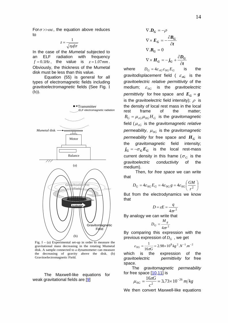
Equation (55) is general for all types of electromagnetic fields including gravitoelectromagnetic fields (See Fig. I (b)).

Acceleration

Gravitoelectric Field

Gravitomagnetic Field

Fig. I – (a) Experimental set-up in order to measure thegravitational mass decreasing in the rotating Mumetal disk. A sample connected to a dynamometer can measurethe decreasing of gravity above the disk. (b)Gravitoelectromagnetic Field.

(b)

(a)

Transmitter ELF electromagnetic radiation

Mumetal disk

Motor

Balance

The Maxwell-like equations for weak gravitational fields are [9]

tD

jH

Bt

BE

D

GGG

G

GG

G

∂∂

+−=×∇

=∇∂

∂−=×∇

−=∇

0.

. ρ

where GGrGG ED 04 εε= is the gravitodisplacement field ( rGε is the gravitoelectric relative permittivity of the medium; G0ε is the gravitoelectric permittivity for free space and gEG = is the gravitoelectric field intensity); ρ is the density of local rest mass in the local rest frame of the matter;

GGrGG HB 0μμ= is the gravitomagnetic field ( rGμ is the gravitomagnetic relative permeability, G0μ is the gravitomagnetic permeability for free space and is the gravitomagnetic field intensity;

GH

GGG Ej σ−= is the local rest-mass current density in this frame ( Gσ is the gravitoelectric conductivity of the medium). Then, for free space we can write that

⎟⎠

⎞⎜⎝

⎛=== 2000 444r

GMgED GGGGG εεε

But from the electrodynamics we know that

24 rqED

πε ==

By analogy we can write that

24 r

MD g

Gπ

=

By comparing this expression with the previous expression of , we get GD

21280 ..1098.2

161 −−×== mNkg

GG πε

which is the expression of the gravitoelectric permittivity for free space. The gravitomagnetic permeability for free space [10,11] is

kgmc

GG

2620 1073316 −×== .πμ

We then convert Maxwell-like equations

15

for weak gravity into a wave equation for free space in the standard way. We conclude that the speed of Gravitational Waves in free space is

cvGG

==00

1με

This means that both electromagnetic and gravitational plane waves propagate at the free space with the same speed. Thus, the impedance for free space is

cGc

HE

Z GGGG

GG

πμεμ 16000 ====

and the Poynting-like vector is GG HESrrr

×=For a plane wave propagating in the vacuum, we have GGG HZE = . Then, it follows that

20

22222

32221

iG

GG

hG

chZ

EZ

Sπωω

===rrr

which is the power per unit area of a harmonic plane wave of angular frequencyω . In classical electrodynamics the density of energy in an electromagnetic field, , has the following expression eW

202

1202

1 HEW rre μμεε +=In analogy with this expression we define the energy density in a gravitoelectromagnetic field, , as follows

GW

202

1202

1GGrGGGrGG HEW μμεε +=

For free space we obtain 1== rGrG εμ

200 1 cGG με =

cHE GGG 0μ=and

GGG HB 0μ=Thus, we can rewrite the equation of as follows

GW

G

G

G

GGG

GG

BBBc

cW

0

22

002

1222

021 1

μμμ

μ=⎟

⎟⎠

⎞⎜⎜⎝

⎛+⎟

⎟⎠

⎞⎜⎜⎝

⎛=

Since VGG WU = , (V is the volume of the particle) and for free space we can write (55) in the following form

1=rn

( )amc

B

mc

Wm

iG

G

iG

g

551121

1121

0

2

20

2

0

2

2

⎪⎭

⎪⎬⎫

⎪⎩

⎪⎨⎧

⎥⎥⎥

⎦

⎤

⎢⎢⎢

⎣

⎡−⎟⎟

⎠

⎞⎜⎜⎝

⎛+−=

⎪⎭

⎪⎬

⎫

⎪⎩

⎪⎨

⎧

⎥⎥⎥

⎦

⎤

⎢⎢⎢

⎣

⎡

−⎟⎟

⎠

⎞

⎜⎜

⎝

⎛+−=

ρμ

ρ

where V0im=ρ . This equation shows how the gravitational mass of a particle is altered by a gravitomagnetic field. A gravitomagnetic field, according to Einstein's theory of general relativity, arises from moving matter (matter current) just as an ordinary magnetic field arises from moving charges. The Earth rotation is the source of a very weak gravitomagnetic field given by

1140 1016

−−≈⎟⎠⎞

⎜⎝⎛−= srad

rMB

Earth

GEarthG .,

ωπ

μ

Perhaps ultra-fast rotating stars can generate very strong gravitomagnetic fields, which can make the gravitational mass of particles inside and near the star negative. According to (55a) this will occur if ρμ GG cB 0061.> . Usually, however, gravitomagnetic fields produced by normal matter are very weak. Recently Tajmar, M. et al., [12] have proposed that in addition to the London moment, ,

(LB

( ) ωω 1110112 −×≅−= .** emBL ; and

are the Cooper-pair mass and charge respectively), a rotating superconductor should exhibit also a large gravitomagnetic field, , to explain an apparent mass increase of Niobium Cooper-pairs discovered by Tate et al[

*m*e

GB

13,14]. According to Tajmar and Matos [15], in the case of coherent matter,

is given by: where GB

202 grGcGB λμωρ−= cρ

is the mass density of coherent matter and grλ is the graviphoton wavelength.

By choosing grλ proportional to the local

density of coherent matter, cρ . i.e.,

16

cGgr

gr

cmρμ

λ 021

=⎟⎟⎠

⎞⎜⎜⎝

⎛=

h

we obtain

ω

ρμμωρλμωρ

2

1220

02

0

−=

=⎟⎟⎠

⎞⎜⎜⎝

⎛−=−=

cGGcgrGcGB

and the graviphoton mass, , is grmcm cGgr hρμ0=

Note that if we take the case of no local sources of coherent matter ( )0=cρ , the graviphoton mass will be zero. However, graviphoton will have non-zero mass inside coherent matter ( )0≠cρ . This can be interpreted as a consequence of the graviphoton gaining mass inside the superconductor via the Higgs mechanism due to the breaking of gauge symmetry. It is important to note that the minus sign in the expression for can be understood as due to the change from the normal to the coherent state of matter, i.e., a switch between real and imaginary values for the particles inside the material when going from the normal to the coherent state of matter. Consequently, in this case the variable U in (55) must be replaced by and not by only. Thus we obtain

GB

GiU GU

( )bmncm

Um ir

i

Gg 551121 0

2

20 ⎪⎭

⎪⎬⎫

⎪⎩

⎪⎨⎧

⎥⎥

⎦

⎤

⎢⎢

⎣

⎡−⎟⎟

⎠

⎞⎜⎜⎝

⎛−−=

Since VGG WU = , we can write (55b) for , in the following form 1=rn

( )cmc

B

mc

Wm

icG

G

ic

Gg

551121

1121

0

2

20

2

0

2

2

⎪⎭

⎪⎬⎫

⎪⎩

⎪⎨⎧

⎥⎥

⎦

⎤

⎢⎢

⎣

⎡−⎟⎟

⎠

⎞⎜⎜⎝

⎛−−=

⎪⎭

⎪⎬⎫

⎪⎩

⎪⎨⎧

⎥⎥

⎦

⎤

⎢⎢

⎣

⎡−⎟⎟

⎠

⎞⎜⎜⎝

⎛−−=

ρμ

ρ

where V0ic m=ρ is the local density of coherent matter. Note the different sign (inside the square root) with respect to (55a).

By means of (55c) it is possible to check the changes in the gravitational mass of the coherent part of a given material (e.g. the Cooper-pair fluid). Thus for the electrons of the Cooper-pairs we have

ieeie

ieeG

ie

ieeG

Giege

mm

mc

m

mc

Bmm

χ

ρμω

ρμ

+=

=⎥⎥⎥

⎦

⎤

⎢⎢⎢

⎣

⎡

⎟⎟⎠

⎞⎜⎜⎝

⎛−−+=

=⎥⎥⎥

⎦

⎤

⎢⎢⎢

⎣

⎡

⎟⎟⎠

⎞⎜⎜⎝

⎛−−+=

2

20

2

2

20

2

4112

112

where eρ is the mass density of the electrons. In order to check the changes in the gravitational mass of neutrons and protons (non-coherent part) inside the superconductor, we must use Eq. (55a) and [Tajmar and

Matos, op.cit.]. Due to ,

that expression of can be rewritten in the following form

202 grGGB λωρμ−=

120 =grcG λρμ

GB

( )cgrGGB ρρωλωρμ 22 20 −=−=

Thus we have

( )

innin

innG

cnin

innG

Gingn

mm

mc

m

mc

Bmm

χ

ρμρρω

ρμ

−=

=⎥⎥⎥

⎦

⎤

⎢⎢⎢

⎣

⎡−⎟

⎟⎠

⎞⎜⎜⎝

⎛+−=

=⎥⎥⎥

⎦

⎤

⎢⎢⎢

⎣

⎡−⎟

⎟⎠

⎞⎜⎜⎝

⎛+−=

14

12

112

2

20

22

2

20

2

( )

ippip

ippG

cpip

ippG

Gipgp

mm

mc

m

mc

Bmm

χ

ρμ

ρρω

ρμ

−=

⎥⎥⎥

⎦

⎤

⎢⎢⎢

⎣

⎡

−⎟⎟

⎠

⎞

⎜⎜

⎝

⎛+−=

=⎥⎥⎥

⎦

⎤

⎢⎢⎢

⎣

⎡−

⎟⎟

⎠

⎞

⎜⎜

⎝

⎛+−=

14

12

112

2

20

22

2

20

2

=

17

where nρ and pρ are the mass density of neutrons and protons respectively. In Tajmar’s experiment, induced accelerations fields outside the superconductor in the order of gμ100 , at

angular velocities of about were observed.

1500 −srad .

Starting from ( ) rGmg initialg= we

can write that ( )( ) rmmGgg ginitialg Δ+=Δ+ .

Then we get rmGg gΔ=Δ . For

( ) rGmgg initialgηη ==Δ it follows that

( ) iinitialgg mmm ηη ==Δ . Therefore a variation of gg η=Δ corresponds to a gravitational mass variation 0ig mm η=Δ .

Thus corresponds to

ggg 4101100 −×=≈Δ μ

04101 ig mm −×≈Δ

On the other hand, the total gravitational mass of a particle can be expressed by

( ) ( )( )

( )( )

( ) 2

2

2

2

2

cENmNmNmNm

cENmNmNmN

cENmNmNmN

cENmmN

mmNmmN

cENmNmNmNm

pieeeipppinnni

pieeeipppinnn

pieeippinn

pieeiee

ippippinninn

pgeegppgnng

Δ+++−=

=Δ+++−

−Δ+++=

=Δ+−+

+−+−

=Δ+++=

χχχ

χχχ

χ

χχ

where EΔ is the interaction energy; , , are the number of neutrons, protons and electrons respectively. Since and

nN pN eN

ipin mm ≅

pn ρρ ≅ it follows that pn χχ ≅ and

consequently the expression of reduces to

gm

( ) ( )dcENmNmNmm pieeeipppig 552 2

0 Δ++−≅ χχ Assuming that ipppieee mNmN χχ 2<< and

ipppp mNcEN χ22 <<Δ Eq. (55d) reduces to

( )emmmNmm ipiipppig 5520 χχ −=−≅ or

00 ipigg mmmm χ−=−=Δ By comparing this expression with

which has been obtained from Tajmar’s experiment, we conclude that at angular velocities

we have

ig mm 4101 −×≈Δ

1500 −≈ srad .ω4101 −×≈pχ

From the expression of we get gpm

( )⎥⎥⎥

⎦

⎤

⎢⎢⎢

⎣

⎡

−⎟⎟

⎠

⎞

⎜⎜

⎝

⎛+=

=⎥⎥⎥

⎦

⎤

⎢⎢⎢

⎣

⎡−

⎟⎟

⎠

⎞

⎜⎜

⎝

⎛+=

14

12

112

2

20

22

2

20

2

c

cB

pG

cp

pG

Gp

ρμ

ρρω

ρμχ

where pVpp m=ρ is the mass density of the protons. In order to calculate pV we need to know the type of space (metric) inside the proton. It is known that there are just 3 types of space: the space of positive curvature, the space of negative curvature and the space of null curvature. The negative type is obviously excluded since the volume of the proton is finite. On the other hand, the space of null curvature is also excluded since the space inside the proton is strongly curved by its enormous mass density. Thus we can conclude that inside the proton the space has positive curvature. Consequently, the volume of the proton, pV , will be expressed by the 3-dimensional space that corresponds to a hypersphere in a 4-dimentional space, i.e., pV will be the space of positive curvature the volume of which is [16]

3222

0 0 0

3 2 pp rdddr πφθχθχππ π

== ∫ ∫ ∫ sinsinpV

In the case of Earth, for example, pEarth ρρ << . Consequently the

curvature of the space inside the Earth is approximately null (space approximately flat). Then

334

EarthEarth rV π≅ .

For we then get mrp151041 −×= .

18

316103 mkgmp

p /×≅=pV

ρ

Starting from the London moment it is easy to see that by precisely measuring the magnetic field and the angular velocity of the superconductor, one can calculate the mass of the Cooper-pairs. This has been done for both classical and high-Tc superconductors [17-20]. In the experiment with the highest precision to date, Tate et al, op.cit., reported a disagreement between the theoretically predicted Cooper-pair mass in Niobium of 99999202 .mm e

* = and its experimental value of ( )210000841. , where is the electron mass. This anomaly was actively discussed in the literature without any apparent solution [

em

21-24]. If we consider that the apparent mass increase from Tate’s measurements results from an increase in the gravitational mass of the

Cooper-pairs due to , then we can write

*gm

GB

( )

***

**

*****

*

**

.

.

.

ii

ii

iginitialggg

i

g

e

g

mm

mm

mmmmm

m

mm

m

χ=×+=

=−=

=−=−=Δ

==

−410840

0000841

00008412

where . 410840 −×= .*χ From (55c) we can write that

***

**

**

ii

iG

ig

mm

mc

mm

χ

ρμω

+=

=⎥⎥⎥

⎦

⎤

⎢⎢⎢

⎣

⎡

⎟⎟⎠

⎞⎜⎜⎝

⎛−−+=

2

20

24112

where is the Cooper-pair mass density.

*ρ

Consequently we can write

42

20

2108404112 −×=

⎥⎥⎥

⎦

⎤

⎢⎢⎢

⎣

⎡

⎟⎟⎠

⎞⎜⎜⎝

⎛−−= .*

*

cG ρμωχ

From this equation we then obtain

316103 mkg /* ×≅ρNote that . *ρρ ≅p

Now we can calculate the graviphoton mass, , inside the Cooper-pairs fluid (coherent part of the superconductor) as

grm

kgcm Ggr

520 104 −×≅= h*ρμ

Outside the coherent matter ( )0=cρ the graviphoton mass will be zero ( )00 == cm cGgr hρμ .

Substitution of pρ , *ρρ =c and

into the expression of

1500 −≈ srad.ω

pχ gives

4101 −×≈pχ

Compare this value with that one obtained from the Tajmar experiment. Therefore, the decrease in the gravitational mass of the superconductor, expressed by (55e), is

SCiSCi

SCipSCiSCg

mm

mmm

,,

,,,

410−−≅

−≅ χ

This corresponds to a decrease of the order of in respect to the initial gravitational mass of the superconductor. However, we must also consider the gravitational shielding effect, produced by this decrease of in the gravitational mass of the particles inside the superconductor (see Fig. II). Therefore, the total weight decrease in the superconductor will be much greater than . According to Podkletnov experiment [

%210−

%210 −≈

%210−

25] it can reach up to 1% of the total weight of the superconductor at 16523 −srad .. ( )rpm5000 . In this experiment a slight decrease (up to

%1≈ ) in the weight of samples hung above the disk (rotating at 5000rpm) was

19

observed. A smaller effect on the order of has been observed when the disk is not rotating. The percentage of weight decrease is the same for samples of different masses and chemical compounds. The effect does not seem to diminish with increases in elevation above the disk. There appears to be a “shielding cylinder” over the disk that extends upwards for at least 3 meters. No weight reduction has been observed under the disk.

%.10

It is easy to see that the decrease in the weight of samples hung above the disk (inside the “shielding cylinder” over the disk) in the Podkletnov experiment, is also a consequence of the Gravitational Shielding Effect showed in Fig. II. In order to explain the Gravitational Shielding Effect, we start with the gravitational field,

μ̂2RGM

g g−=r

, produced by a particle

with gravitational mass, . The

gravitational flux,gM

gφ , through a spherical

surface, with area and radius S R , concentric with the mass , is given by

gM

( ) gg

SSg

GMRR

GM

SgdSgSdg

ππ

φ

44 22 ==

==== ∫∫rr

Note that the flux gφ does not depend on the radius R of the surface , i.e., it is the same through any surface concentric with the mass .

S

gM Now consider a particle with gravitational mass, , placed into the

gravitational field produced by . According to Eq. (41), we can have

gm′

gM

10 −=′′ ig mm , 00 ≅′′ ig mm †, 10 =′′ ig mm , etc. In the first case, the gravity † The quantization of the gravitational mass (Eq.(33)) shows that for n = 1 the gravitational mass is not zero but equal to mg(min).Although the gravitational mass of a particle is never null, Eq.(41) shows that it can be turned very close to zero.

acceleration, g ′ , upon the particle gm′ ,

is μ̂2RGM

gg g+=−=′r . This means that

in this case, the gravitational flux, gφ ′ ,

through the particle will be given by gm′

gg gSSg φφ −=−=′=′ , i.e., it will be symmetric in respect to the flux when

0ig mm ′=′ (third case). In the second case

( )0≅′gm , the intensity of the

gravitational force between and will be very close to zero. This is equivalent to say that the gravity acceleration upon the particle with mass

gm′ gM

gm′ will be 0≅′g . Consequently we can

write that 0≅′=′ Sggφ . It is easy to see that there is a correlation between

0ig mm ′′ and gg φφ′ , i.e., _ If 10 −=′′ ig mm ⇒ 1−=′ gg φφ _ If 10 =′′ ig mm ⇒ 1=′ gg φφ _ If 00 ≅′′ ig mm ⇒ 0≅′ gg φφ Just a simple algebraic form contains the requisites mentioned above, the correlation

0i

g

g

g

mm

′

′=

′

φφ

By making χ=′′ 0ig mm we get

gg φχφ =′ This is the expression of the gravitational flux through gm′ . It explains the Gravitational Shielding Effect presented in Fig. II. As gSg =φ and Sgg ′=′φ , we obtain

gg χ=′ This is the gravity acceleration inside gm′ . Figure II (b) shows the gravitational shielding effect produced by two particles at the same direction. In this case, the

20

gravity acceleration inside and above the second particle will be ifg2χ 12 ig mm = . These particles are representative of any material particles or material substance (solid, liquid, gas, plasma, electrons flux, etc.), whose gravitational mass have been reduced by the factor χ . Thus, above the substance, the gravity acceleration is reduced at the same proportion

g ′

0ig mm=χ , and,

consequently, gg χ=′ , where is the gravity acceleration below the substance.

g

Figure III shows an experimental set-up in order to check the factor χ above a high-speed electrons flux. As we have shown (Eq. 43), the gravitational mass of a particle decreases with the increase of the velocity V of the particle. Since the theory says that the factor χ is given by the correlation

0ig mm then, in the case of an electrons

flux, we will have that iege mm=χ where

as function of the velocity V is given by Eq. (43). Thus, we can write that

gem

⎪⎭

⎪⎬⎫

⎪⎩

⎪⎨⎧

⎥⎥⎦

⎤

⎢⎢⎣

⎡−

−−== 1

1

12122 cVm

m

ie

geχ

Therefore, if we know the velocity V of the electrons we can calculate χ . ( is the electron mass at rest).

iem

When an electron penetrates the electric field (see Fig. III) an electric

force,yE

yE EeFrr

−= , will act upon the

electron. The direction of will be

contrary to the direction ofEFr

yEr

. The

magnetic force which acts upon the

electron, due to the magnetic fieldBFr

Br

, is and will be opposite to μ̂eVBFB =

rEFr

because the electron charge is negative. By adjusting conveniently B we can make EB FF

rr= . Under these

circumstances in which the total force is zero, the spot produced by the electrons

flux on the surface α returns from O′ to and is detected by the

galvanometerG . That is, there is no deflection for the cathodic rays. Then it follows that

O

yeEeVB = since EB FFrr

= .

Then, we get

BE

V y=

This gives a measure of the velocity of the electrons. Thus, by means of the experimental set-up, shown in Fig. III, we can easily obtain the velocity V of the electrons below the body β , in order to calculate the theoretical value of χ . The experimental value of χ can be obtained by dividing the weight, gmg ′P =′β β of

the body β for a voltage drop V~ across the anode and cathode, by its weight, gPβ mgβ= , when the voltage

V~ is zero, i.e.,

gg

PP ′

=′

=β

βχ

According to Eq. (4), the gravitational mass, , is defined by gM

221 cV

mM g

g−

=

While Eq. (43) defines by means of the following expression

gm

0221

1

121 ig mcV

m⎪⎭

⎪⎬⎫

⎪⎩

⎪⎨⎧

⎥⎥⎦

⎤

⎢⎢⎣

⎡−

−−=

In order to check the gravitational mass of the electrons it is necessary to know the pressure produced by the electrons flux. Thus, we have put a piezoelectric sensor in the bottom of the glass tube as shown in Fig. III. The electrons flux radiated from the cathode is accelerated by the anode1 and strikes on the piezoelectric sensor yielding a pressure

P

P which is measured by means of the sensor.

21

Fig. I I – The Gravitational Shielding effect.

(a)

mg = mi mg < mi mg < 0

(b)

g′ < g due to the gravitational shielding effect produced by mg 1

Particle 1 mg 1

Particle 2 mg 2

mg 1 = x mi 1 ; x < 1

g′

g

P2 = mg 2 g′ = mg 2 ( x g )

P1 = mg 1 g = x mi 1 g

g g g

g′ < g g g′ < 0

22

Let us now deduce the correlation between P and . geM When the electrons flux strikes the sensor, the electrons transfer to it a momentum . Since

VMnqnQ geeee ==

VFdtFQ 2=Δ= , we conclude that

⎟⎟⎠

⎞⎜⎜⎝

⎛=

ege n

FV

dM 2

2

The amount of electrons, , is given by

enSdne ρ= where ρ is the amount of

electrons per unit of volume (electrons/m

3); is the cross-section

of the electrons flux and the distance between cathode and anode.

Sd

In order to calculate we will start from the Langmuir-Child law and the Ohm vectorial law, respectively given by

en

dVJ

23~

α= and VJ cρ= , ( )ec ρρ =

where is the thermoionic current density;

J23

1610332 −−−×= VmA ...α is the called Child’s constant; V~ is the voltage drop across the anode and cathode electrodes, and V is the velocity of the electrons. By comparing the Langmuir-Child law with the Ohm vectorial law we obtain

VedV

2

23~αρ =

Thus, we can write that

edVSVne

23~α

=

and

PVV

edM ge ⎟⎟⎠

⎞⎜⎜⎝

⎛=

23

22~α

Where SFP = , is the pressure to be measured by the piezoelectric sensor. In the experimental set-up the total force acting on the

piezoelectric sensor is the resultant of all the forces produced by each electrons flux that passes through each hole of area in the grid of the anode 1, and is given by

F

φF

φS

( ) 23

22VVM

ednS

PSnnFF ge~

⎟⎟⎠

⎞⎜⎜⎝

⎛=== φ

φφ

α

where is the number of holes in the grid. By means of the piezoelectric sensor we can measure and consequently obtain .

n

FgeM

We can use the equation above to evaluate the magnitude of the force to be measured by the piezoelectric sensor. First, we will find the expression of V as a function of

F

V~ since the electrons speed V depends on the voltage V~ . We will start from Eq. (46) which is the general expression for Lorentz’s force, i.e.,

( )0i

g

mm

BVqEqdtpd rrrr

×+=

When the force and the speed have the same direction Eq. (6) gives

( ) dtVd

cV

mdtpd g

rr

23

221−=

By comparing these expressions we obtain

( )BVqEq

dtVd

cV

mirrr

r

×+=− 2

322

0

1In the case of electrons accelerated by a sole electric field , the equation above gives

( 0=B )

( )ieie mVecV

mEe

dtVda

~21 22−==rr

r

Therefore, the velocity V of the electrons in the experimental set-up is

( )iemVecVadV~212 4

322−==

From Eq. (43) we conclude that

23

Dynamometer (D)

Fig. III – Experimental set-up in order to check the factor χ above a high-speed electrons flux. The set-up may also check the velocities and the gravitational masses of the electrons.

G

- +

V~

B+ yV~

−

Eyy

O’

⋅

α + γ

↓iG

R

F e V e O

+ −

Anode 1 Filaments Cathode Anode 2 Piezoelectric sensor

β d Collimators g’= χ g ↓g Grid d Collimators

24

0≅gem when . Substitution

of this value of V into equation above givesV

cV 7450.≅

KV1479.~ ≅ . This is the voltage drop necessary to be applied across the anode and cathode electrodes in order to obtain 0≅gem . Since the equation above can be used to evaluate the velocity V of the electrons flux for a givenV~ , then we can use the obtained value of V to evaluate the intensity of B

rin order to

produce yeEeVB = in the experimental set-up. Then by adjusting B we can check when the electrons flux is detected by the galvanometer . In this case, as we have already seen, , and the velocity of the electrons flux is calculated by means of the expression

GyeEeVB =

BEV y= . Substitution of into the expressions of and

, respectively given by V gem

geM

iege mcV

m⎪⎭

⎪⎬⎫

⎪⎩

⎪⎨⎧

⎥⎥⎦

⎤

⎢⎢⎣

⎡−

−−= 1

1

12122

and

221 cV

mM ge

ge−

=

yields the corresponding values of and which can be compared

with the values obtained in the experimental set-up:

gem geM

( )

⎟⎟⎠

⎞⎜⎜⎝

⎛=

′==

φ

ββ

α

χ

nSed

VV

FM

mPPmm

ge

ieiege

22~ 2

3

where and are measured by the dynamometer and is measured by the piezoelectric sensor.

βP′ βPD F

If we have and 2160 mnS .≅φ

md 080.= in the experimental set-up then it follows that

23

1410821 VVMF ge~. ×=

By varying V~ from 10KV up to 500KV we note that the maximum value for

occurs when F KVV 7344.~ ≅ . Under these circumstances, and cV 70.≅

iege mM 280.≅ . Thus the maximum value for is F

gfNF 19091 ≅≅ .max

Consequently, for KVV 500=max~ , the

piezoelectric sensor must satisfy the following characteristics:

− Capacity 200gf − Readability 0.001gf Let us now return to the explanation for the findings of Podkletnov’s experiment. Next, we will explain the decrease of 0.1% in the weight of the superconductor when the disk is only levitating but not rotating. Equation (55) shows how the gravitational mass is altered by electromagnetic fields. The expression of for rn

ωεσ >> can be obtained from (54), in the form

( )564

2

fc

vcnr π

μσ==

Substitution of (56) into (55) leads to

0

2

14

121 ii

g mcm

Uf

m⎪⎭

⎪⎬⎫

⎪⎩

⎪⎨⎧

⎥⎥

⎦

⎤

⎢⎢

⎣

⎡−⎟⎟

⎠

⎞⎜⎜⎝

⎛+−=

πμσ

This equation shows that atoms of ferromagnetic materials with very-high μ can have gravitational masses strongly reduced by means of Extremely Low Frequency (ELF) electromagnetic radiation. It also shows that atoms of superconducting

25

materials (due to very-high σ ) can also have its gravitational masses strongly reduced by means of ELF electromagnetic radiation. Alternatively, we may put Eq.(55) as a function of the power density ( or intensity ), , of the radiation. The integration of (51) gives

D

vDU V= . Thus, we can write (55) in the following form:

( )571121 0

2

3

2

ir

g mcDn

m⎪⎭

⎪⎬⎫

⎪⎩

⎪⎨⎧

⎥⎥

⎦

⎤

⎢⎢

⎣

⎡−⎟⎟

⎠

⎞⎜⎜⎝

⎛+−=

ρ

where V0im=ρ . For ωεσ >> , will be given by (56) and consequently (57) becomes

rn

( )5814

121 0

2

ig mcf

Dm⎪⎭

⎪⎬⎫

⎪⎩

⎪⎨⎧

⎥⎥

⎦

⎤

⎢⎢

⎣

⎡−⎟⎟

⎠

⎞⎜⎜⎝

⎛+−=

ρπμσ

In the case of Thermal radiation, it is common to relate the energy of photons to temperature, T, through the relation,

Thf κ≈

where is the Boltzmann’s constant. On the other hand it is known that

KJ °×= − /. 2310381κ

4TD Bσ=

where 42810675 KmwattsB °×= − /.σis the Stefan-Boltzmann’s constant. Thus we can rewrite (58) in the following form

( )amc

hTm i

Bg 581

4121 0

23

⎪⎭

⎪⎬

⎫

⎪⎩

⎪⎨

⎧

⎥⎥⎥

⎦

⎤

⎢⎢⎢

⎣

⎡−⎟

⎟⎠

⎞⎜⎜⎝

⎛+−=

πκρμσσ

Starting from this equation, we can evaluate the effect of the thermal radiation upon the gravitational mass of the Copper-pair fluid, . Below the transition temperature, ,

CPfluidgm ,

cT( 50.<cTT ) the conductivity of the superconducting materials is usually larger than [mS /2210 26]. On the

other hand the transition temperature, for high critical temperature (HTC) superconducting materials, is in the order of . Thus (58a) gives K210

( )bmm CPfluidiCPfluid

CPfluidg 58110~121 ,2

9

,⎪⎭

⎪⎬⎫

⎪⎩

⎪⎨⎧

⎥⎥⎦

⎤

⎢⎢⎣

⎡−+−=

−

ρ

Assuming that the number of Copper-pairs per unit volume is [

32610 −≈ mN27] we can write that

3410 mkgNmCPfluid /* −≈=ρSubstitution of this value into (58b) yields

CPfluidiCPfluidiCPfluidg mmm ,,, 1.0−=

This means that the gravitational masses of the electrons are decreased of ~10%. This corresponds to a decrease in the gravitational mass of the superconductor given by

( )( )

999976.0

9.02

2

2

2

2

2

,

,

=

=⎟⎟⎠

⎞⎜⎜⎝

⎛

Δ+++

Δ+++=

=⎟⎟⎠

⎞⎜⎜⎝

⎛

Δ+++

Δ+++=

=Δ+++

Δ+++=

cEmmmcEmmm

cEmmmcEmmm

cEmmmNcEmmmN

mm

inipie

inipie

inipie

gngpge

inipie

gngpge

SCi

SCg

Where EΔ is the interaction energy. Therefore, a decrease of ( ) 51099997601 −≈− . , i.e., approximately

in respect to the initial gravitational mass of the superconductor, due to the local thermal radiation only. However, here we must also consider the gravitational shielding effect produced, in this case, by the decrease of in the gravitational mass of the particles inside the superconductor (see Fig. II). Therefore the total weight decrease in the superconductor will

%310−

%310 −≈

26

be much greater than . This can explain the smaller effect on the order of observed in the Podkletnov measurements when the disk is not rotating.

%310 −≈

%.10

Let us now consider an electric current I through a conductor subjected to electromagnetic radiation with power density and frequency .

Df

Under these circumstances the gravitational mass of the electrons of the conductor, according to Eq. (58), is given by

gem

ege mcf

Dm⎪⎭

⎪⎬⎫

⎪⎩

⎪⎨⎧

⎥⎥

⎦

⎤

⎢⎢

⎣

⎡−⎟⎟

⎠

⎞⎜⎜⎝

⎛+−= 1

4121

2

ρπμσ

where . kg.me3110119 −×=

Note that if the radiation upon the conductor has extremely-low frequency (ELF radiation) then can be strongly reduced. For example, if , and the conductor is made of copper (

gem

Hzf 610−≈ 2510 m/WD ≈

0μμ ≅ ; and) then

m/S. 71085 ×=σ38900 m/kg=ρ

14

≈⎟⎟⎠

⎞⎜⎜⎝

⎛cf

Dρπ

μσ

and consequently . ege m.m 10≈ According to Eq. (6) the force upon each free electron is given by

( )Ee

dtVd

cV

mF ge

e

rr

r=

−=

23221

where E is the applied electric field. Therefore, the decrease of produces an increase in the velocity

of the free electrons and consequently the drift velocity is also increased. It is known that the density of electric current through a conductor [

gem

VdV

J28] is given by

deVJrr

Δ=where eΔ is the density of the free electric charges ( For cooper conductors ). Therefore increasing produces an increase in the electric current

3101031 m/C.e ×=Δ

dVI .

Thus if is reduced 10 times gem( )ege m.m 10≈ the drift velocity is increased 10 times as well as the electric current. Thus we conclude that strong fluxes of ELF radiation upon electric/electronic circuits can suddenly increase the electric currents and consequently damage these circuits.

dV

Since the orbital electrons moment of inertia is given by ( ) 2

jjii rmI Σ= , where refers to inertial mass and not to gravitational mass, then the momentum

im

ωiIL = of the conductor orbital electrons are not affected by the ELF radiation. Consequently, this radiation just affects the conductor’s free electrons velocities. Similarly, in the case of superconducting materials, the momentum, ωiIL = , of the orbital electrons are not affected by the gravitomagnetic fields. The vector ( )vUD rr

V= , which we may define from (48), has the same direction of the propagation vector k

r

and evidently corresponds to the Poynting vector. Then can be replaced by

Dr

HErr

× .Thus we can write ( ) ( )[ ] ( ) 2

21

21

21

21 1 EvvEEBEEHD μμμ ==== .

For ωεσ >> Eq. (54) tells us that μσπfv 4= . Consequently, we obtain

μπσf

ED4

221=

This expression refers to the instantaneous values of and D E . The average value for 2E is equal to

22

1mE because E varies sinusoidaly

27

( is the maximum value for mE E ). Substitution of the expression of into (58) gives

D

( )amE

fcm ig 591

44121 02

23

2⎪⎭

⎪⎬⎫

⎪⎩

⎪⎨⎧

⎥⎥

⎦

⎤

⎢⎢

⎣

⎡−⎟⎟

⎠

⎞⎜⎜⎝

⎛+−=

ρπσμ

Since 2mrms EE = and 2212

mEE = we can write the equation above in the following form

( )amE

fcm i

rmsg 591

44121 02

23

2⎪⎭

⎪⎬⎫

⎪⎩

⎪⎨⎧

⎥⎥

⎦

⎤

⎢⎢

⎣

⎡−⎟⎟

⎠

⎞⎜⎜⎝

⎛+−=

ρπσμ

Note that for extremely-low frequencies the value of in this equation becomes highly expressive.

3−f

Since equation (59a) can also be put as a function of

vBE =B ,

i.e.,

( )bmBcf

m ig 5914

121 02

4

2⎪⎭

⎪⎬⎫

⎪⎩

⎪⎨⎧

⎥⎥⎦

⎤

⎢⎢⎣

⎡−⎟⎟

⎠

⎞⎜⎜⎝

⎛+−=

ρμπσ

For conducting materials with ; m/S710≈σ 1=rμ ;

the expression (59b) gives

3310 m/kg≈ρ

04

12

110121 ig mBf

m⎪⎭

⎪⎬⎫

⎪⎩

⎪⎨⎧

⎥⎥⎦

⎤

⎢⎢⎣

⎡−⎟⎟

⎠

⎞⎜⎜⎝

⎛ ≈+−=

−

This equation shows that the decreasing in the gravitational mass of these conductors can become experimentally detectable for example, starting from 100Teslas at 10mHz. One can then conclude that an interesting situation arises when a body penetrates a magnetic field in the direction of its center. The gravitational mass of the body decreases progressively. This is due to the intensity increase of the magnetic field upon the body while it penetrates the field. In order to understand this phenomenon we might, based on (43), think of the inertial mass as being formed by two parts: one positive and another negative. Thus, when the body

penetrates the magnetic field, its negative inertial mass increases, but its total inertial mass decreases, i.e., although there is an increase of inertial mass, the total inertial mass (which is equivalent to gravitational mass) will be reduced. On the other hand, Eq.(4) shows that the velocity of the body must increase as consequence of the gravitational mass decreasing since the momentum is conserved. Consider for example a spacecraft with velocity and gravitational mass . If is reduced to then the velocity becomes

sV

gM gM gm

( ) sggs VmMV =′

In addition, Eqs. 5 and 6 tell us that the inertial forces depend on . Only in the particular case of

gm

0ig mm = the expressions (5) and (6) reduce to the well-known Newtonian expression . Consequently, one can conclude that the inertial effects on the spacecraft will also be reduced due to the decreasing of its gravitational mass. Obviously this leads to a new concept of aerospace flight.

amF i 0=

Now consider an electric current ftsinii π20= through a conductor. Since the current density, Jr

, is expressed by ESddiJrrr

σ== , then we can write that

( ) ftsinSiSiE πσσ 20== . Substitution of this equation into (59a) gives

( )cmftfSc

im ig 591264

121 04

34223

40

⎪⎭

⎪⎬⎫

⎪⎩

⎪⎨⎧

⎥⎥⎦

⎤

⎢⎢⎣

⎡−+−= π

σρπμ sin

If the conductor is a supermalloy rod ( )mm40011 ×× then 000100,r =μ (initial); ; and . Substitution of these values into the equation above yields the following expression for the

38770 m/kg=ρ m/S. 61061 ×=σ26101 mS −×=

28

gravitational mass of the supermalloy rod

( ) ( ) ( )smismg mftfim⎭⎬⎫

⎩⎨⎧

⎥⎦⎤

⎢⎣⎡ −×+−= − 12sin1071.5121 434

012 π

Some oscillators like the HP3325A (Op.002 High Voltage Output) can generate sinusoidal voltages with extremely-low frequencies down to

and amplitude up to 20V (into

Hzf 6101 −×=Ω50 load). The maximum

output current is . ppA.080 Thus, for ( )ppA.A.i 0800400 =

and the equation above shows that the gravitational mass of the rod becomes negative at

Hz.f 610252 −×<

22 ππ =ft ; for at Hz.f 61071 −×≅h.s.ft 8401047141 5 ≅×== it shows

that . ( ) ( )smismg mm −≅ This leads to the idea of the Gravitational Motor. See in Fig. IV a type of gravitational motor (Rotational Gravitational Motor) based on the possibility of gravity control on a ferromagnetic wire. It is important to realize that this is not the unique way of decreasing the gravitational mass of a body. It was noted earlier that the expression (53) is general for all types of waves including non-electromagnetic waves like sound waves for example. In this case, the velocity v in (53) will be the speed of sound in the body and the intensity of the sound radiation. Thus from (53) we can write that

D

2cvD

cmD

cmp

ii ρΔ

==V

It can easily be shown that wherevAfD 2222 ρπ= 22 vPA πρλ= ;

A and P are respectively the amplitude and maximum pressure variation of the sound wave. Therefore we readily obtain

32

2

0 2 cvP

cmp

i ρ=

Δ

Substitution of this expression into (41) gives

( )6012

121 0

2

32

2

ig mcv

Pm⎪⎭

⎪⎬

⎫

⎪⎩

⎪⎨

⎧

⎥⎥⎥

⎦

⎤

⎢⎢⎢

⎣

⎡−⎟

⎟⎠

⎞⎜⎜⎝

⎛+−=

ρ

This expression shows that in the case of sound waves the decreasing of gravitational mass is relevant for very strong pressures only. It is known that in the nucleus of the Earth the pressure can reach values greater than . The equation above tells us that sound waves produced by pressure variations of this magnitude can cause strong decreasing of the gravitational mass at the surroundings of the point where the sound waves were generated. This obviously must cause an abrupt decreasing of the pressure at this place since pressure = weight /area = m

21310 m/N

gg/area). Consequently a local instability will be produced due to the opposite internal pressure. The conclusion is that this effect may cause Earthquakes. Consider a sphere of radius r around the point where the sound waves were generated (at depth; the Earth's radius is ). If the maximum pressure, at the explosion place ( sphere of radius ), is and the pressure at the distance is

km,0001≈km,3786

0r21310 m/NPmax ≈

kmr 10=( ) 292

0 10 m/NPrrP maxmin ≈= then we can consider that in the sphere

21110 m/NPPP minmax ≈= .Thus assuming

and we can calculate the variation of gravitational mass in the sphere by means of the equation of , i.e.,

s/mv 310≈ 3310 m/kg≈ρ

gm

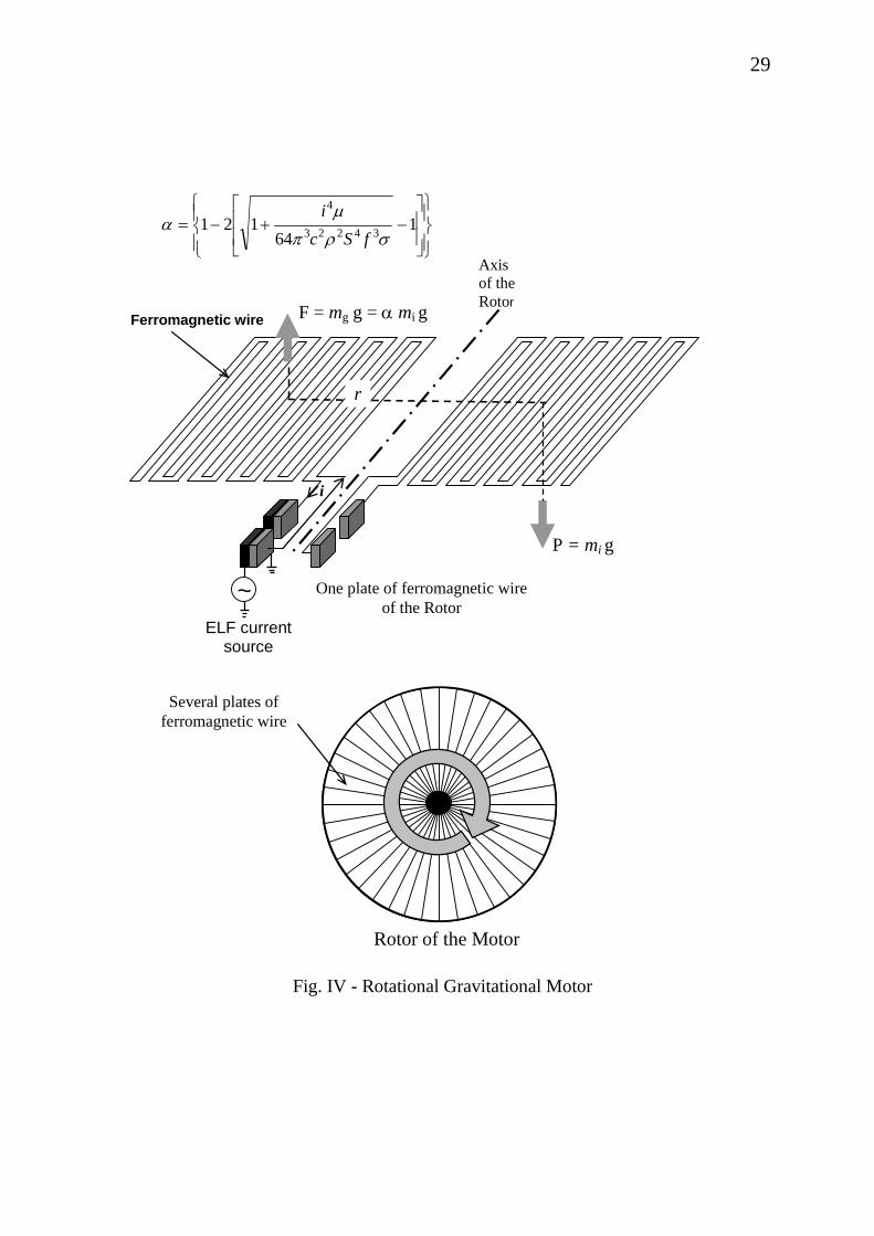
29

Fig. IV - Rotational Gravitational Motor

One plate of ferromagnetic wireof the Rotor

~

Axis of the Rotor

r

F = mg g = α mi g Ferromagnetic wire

P = mi g

i

Several plates of ferromagnetic wire

Rotor of the Motor

⎪⎭

⎪⎬⎫

⎪⎩

⎪⎨⎧

⎥⎥

⎦

⎤

⎢⎢

⎣

⎡−+−= 1

64121 34223

4

σρπμ

αfSc

i

ELF current source

30

( )

kgVcv

P

mcv

Pm

mmm

ii

ginitialgg

112

32

2

0

2

32

2

0

1012

12

12

121

≈⎥⎥

⎦

⎤

⎢⎢

⎣

⎡−⎟⎟

⎠

⎞⎜⎜⎝

⎛+=

=⎪⎭

⎪⎬⎫

⎪⎩

⎪⎨⎧

⎥⎥

⎦

⎤

⎢⎢

⎣

⎡−⎟⎟

⎠

⎞⎜⎜⎝

⎛+−−=

=−=Δ

ρρ

ρ

The transitory loss of this great amount of gravitational mass may evidently produce a strong pressure variation and consequently a strong Earthquake. Finally, we can evaluate the energy necessary to generate those sound waves. From (48) we can write

. Thus, the released power is

21610 m/WvPD maxmax ≈=

( ) WrDP max212

00 104 ≈= π and the energy EΔ released at the time interval tΔ must be tPE ΔΔ 0= . Assuming we readily obtain st 310−≈Δ

MegatonsjoulestPE 4180 1010 ≈≈= ΔΔ

This is the amount of energy released by an earthquake of magnitude 9

), i.e.,( 9=sM ( ) joules.E sM. 184415 1010741 ≅×= + . The maximum magnitude in the Richter scale is 12. Note that the sole releasing of this energy at 1000km depth (without the effect of gravitational mass decreasing) cannot produce an Earthquake, since the sound waves reach 1km depth with pressures less than 10N/cm2. Let us now return to the Theory. The equivalence between frames of non-inertial reference and gravitational fields assumed ig mm ≡ because the inertial forces were given by amF ii

rr= , while the equivalent

gravitational forces, by gmF ggrr

= . Thus, to satisfy the equivalence ( and ga rr

≡ gi FF ≡r

) it was necessary that . Now, the inertial

force,

ig mm ≡

iFr

, is given by Eq.(6), and from Eq.(13) we can obtain the gravitational force, gF

r. Thus, gi FF

rr≡

leads to

( )

( ) ( )( )61

11

111

23

23

23

22222

2222222

cV

mg

cV

m

r

mG

cV

m

cVr

mGa

cV

m

ggg

ggg

−≡

−⎟⎟⎠

⎞⎜⎜⎝

⎛′

′≡

≡−⎟

⎠⎞⎜

⎝⎛ −′

′≡

−

r

r

whence results ( )62ga rr

≡Consequently, the equivalence is evident, and therefore Einstein's equations from the General Relativity continue obviously valid. The new expression for (Eqs. (5) and (6)) shows that the inertial forces are proportional to the gravitational mass, . This means that these forces result from the gravitational interaction between the particle and the other gravitational masses of the Universe, just as Mach’s principle predicts. Therefore the new expression for the inertial forces incorporates the Mach’s principle into Gravitation Theory, and furthermore reveals that the inertial effects upon a particle can be reduced because, as we have seen, the gravitational mass may be reduced. When the nonrelativistic equation for inertial forces,

iF

gm

0ig mm =

amF girr

= , reduces to

amF iirr

0= . This is the well-known Newton's second law for motion. In Einstein's Special Relativity Theory the motion of a free-particle is described by means of 0=Sδ [29]. Now based on Eq. (1), 0=Sδ will be given by the following expression

( )63.0∫ =−= dscmS g δδ

which also describes the motion of the particle inside the gravitational

31

field. Thus, Einstein's equations from the General Relativity can be derived starting from ( ) 0=+ gm SSδ , where

and refer to the action of the gravitational field and the action of the matter, respectively [

gS mS

30]. gS The variations δ and mSδ can

be written as follows [31]:

( ) ( )6416 2

13

Ω−−= ∫ dggRgRG

cS ikikikg δ

πδ

( )6521

Ω−−= ∫ dggTc

S ikikm δδ

where is the Ricci's tensor; the metric tensor and the matter's energy-momentum tensor:

ikR ikg

ikT

( ) ( )66ikkigik PgPT ++= μμε

where P is the pressure and is now, the density of gravitational energy, , of the particle;

2cgg ρε =

gE gρ is then the density of gravitational mass of the particle, i.e., at the volume unit.

gM

Substitution of (64) and (65) into 0=+ gm SS δδ yields

( ) 016 4

821

3

=−−−∫ Ωδπ

π dggTRgRG

c ikikc

Gikik

whence, ( )6704

821 =⎟

⎠⎞⎜

⎝⎛ −− ikc

Gikik TRgR π

because the ikgδ are arbitrary. Equations (67) in the following form

( )6848

21

ikcG

ikik TRgR π=−

or ( )69.4

821 k

icGk

iki TRgR πδ =−

are the Einstein's equations from the General Relativity. It is known that these equations are only valid if the spacetime is continuous. We have shown at the beginning of this work that the spacetime is not continuous it is quantized. However, the spacetime can be considered approximately “continuous” when the quantum

number is very large (Classical limit). Therefore, just under these circumstances the Einstein's equations from the General Relativity can be used in order to “classicalize” the quantum theory by means of approximated description of the spacetime.

n

Later on we will show that the length of Eq. (29) is given by mind

( ) ( )7010~~ 343min

21

mcGklkd planck−≈== h

(See Eq. (100)). On the other hand, we will find in the Eq. (129) the length scale of the initial Universe, i.e.,

. Thus, from the Eq. (29) we get:

mdinitial1410−≈

203414min 101010 ≈== −−ddn initial

this is the quantum number of the spacetime at initial instant. That quantum number is sufficiently large for the spacetime to be considered approximately “continuous” starting from the beginning of the Universe. Therefore Einstein's equations can be used even at the Initial Universe. Now, it is easy to conclude why the attempt to quantize gravity starting from the General Relativity was a bad theoretical strategy. Since the gravitational interaction can be repulsive, besides attractive, such as the electromagnetic interaction, then the graviton must have spin 1 (called graviphoton) and not 2. Consequently, the gravitational forces are also gauge forces because they are yielded by the exchange of the so-called "virtual" quanta of spin 1, such as the electromagnetic forces and the weak and strong nuclear forces. Let us now deduce the Entropy Differential Equation starting from Eq. (55). Comparison of Eqs. (55) and (41) shows that pcUnr Δ= . For small velocities, i.e., ( )cV << , we have

. Under these 20cmUn ir <<

32

circumstances, the development of Eq. (55) in power of ( )2

0cmUn ir gives

( )710

2

20

0 ii

rig m

cmUn

mm ⎟⎟⎠

⎞⎜⎜⎝

⎛−=

In the particular case of thermal radiation, it is usual to relate the energy of the photons to the temperature, through the relationship

kTh ≈ν where KJ.k 2310381 −×= is the Boltzmann's constant. Thus, in that case, the energy absorbed by the particle will be kThU ηνη ≈= , where η is a particle-dependent absorption/emission coefficient. Therefore, Eq.(71) may be rewritten in the following form:

( )72020

22

20 ii

rig m

mT

ckn

mm⎥⎥⎦

⎤

⎢⎢⎣

⎡⎟⎠

⎞⎜⎝

⎛−=η

For electrons at T=300K, we have

172

22

2 10−≈⎟⎠⎞

⎜⎝⎛

e

r

mT

ckn η

Comparing (72) with (18), we obtain

( )7321

0

22

.i

rKi m

Tc

knE ⎟⎠

⎞⎜⎝

⎛=η

The derivative of with respect to temperature T is

KiE

( ) ( ) (7402

irKi mTckn

TE

η=∂

∂ )Thus,

( ) ( )752

0

2

cmkTn

TE

Ti

rKi η=

∂∂

Substitution of into (75) gives

0iiKi EEE −=

( ) ( )7620

20

cmkTn

TE

TE

Ti

rii η=⎟

⎠

⎞⎜⎝

⎛∂

∂+

∂∂

By comparing the Eqs.(76) and (73) and considering that 00 =∂∂ TEi because does not depend on 0iE T , the Eq.(76) reduces to

( ) ( )772 Kii ETET =∂∂ However, Eq.(18) shows that

giKi EEE −=2 .Therefore Eq.(77) becomes ( ) ( )78TETEE iig ∂∂−=

Here, we can identify the energy with the free-energy of the system-F and with the internal energy of the system-U. Thus we can write the Eq.(78) in the following form:

iE

gE

( ) ( )79TFTFU ∂∂−=This is the well-known equation of Thermodynamics. On the other hand, remembering that UQ ∂+∂=∂ τ (1st

principle of Thermodynamics) and ( )80TSUF −=

(Helmholtz's function), we can easily obtain from (79), the following equation

( )81.STQ ∂+∂=∂ τFor isolated systems, 0=∂τ , we have

( )82STQ ∂=∂which is the well-known Entropy Differential Equation. Let us now consider the Eq.(55) in the ultra-relativistic case where the inertial energy of the particle is much larger than its inertial energy at rest . Comparison of (4) and (10) leads to

2cME ii =2

0cmi

2cVEp i=Δ which, in the ultra-relativistic case, gives

cMcEcVEp iii ≅≅= 2Δ . On the other hand, comparison of (55) and (41) shows that pcUnr Δ= . Thus

. Consequently, Eq.(55) reduces to

20

2 cmcMpcUn iir >>≅Δ=

( )832 2

0 cUnmm rig −=

Therefore, the action for such particle, in agreement with the Eq.(2), is

33

( )[ ( )84121

12

1

2

1

2

1

2

1

22222

2222

222

∫

∫

∫

−+−−=

=−+−=

=−−=

t

t ri

t

t ri

t

t g

.dtcVUncVcm

dtcVccUnm

dtcVcmS

]The integrant function is the Lagrangean, i.e.,

( )85121 222220 cVUncVcmL ri −+−−=

Starting from the Lagrangean we can find the Hamiltonian of the particle, by means of the well-known general formula:

( ) .LVLVH −∂∂=The result is

( ) ( )861

24

1 22

22

22

20 .

⎥⎥⎦

⎤

⎢⎢⎣

⎡

−

−+

−=

cV

cVUncV

cmH r

i

The second term on the right hand side of Eq.(86) results from the particle's interaction with the electromagnetic field. Note the similarity between the obtained Hamiltonian and the well-known Hamiltonian for the particle in an electromagnetic field [32]:

( )871 2220 .ϕQcVcmH i +−=

in which is the electric charge and Qϕ , the field's scalar potential. The quantity ϕQ expresses, as we know, the particle's interaction with the electromagnetic field in the same way as the second term on the right hand side of the Eq. (86). It is therefore evident that it is the same quantity, expressed by different variables. Thus, we can conclude that, in ultra-high energy conditions ( )2

02 cmcMUn iir >≅ , the gravitational

and electromagnetic fields can be described by the same Hamiltonian, i.e., in these circumstances they are unified ! It is known that starting from that Hamiltonian we may obtain a

complete description of the electromagnetic field. This means that from the present theory for gravity we can also derive the equations of the electromagnetic field. Due to the second term on the right hand side of Eq.(86) can be written as follows

2cMpcUn ir ≅= Δ

( )

( )

2200

2

22

22

22

22

144

1

24

1

24

cVr

QQR

QQQ

cMcV

cV

cV

cVpc

i

−

′=

′==

=⎥⎥⎦

⎤

⎢⎢⎣

⎡

−

−=

=⎥⎥⎦

⎤

⎢⎢⎣

⎡

−

−

πεπεϕ

Δ

whence

( )r

QQcMcV i0

222

424

πε′

=−

The factor ( )24 22 −cV becomes equal to 2 in the ultra-relativistic case, then it follows that

( )884

20

2

rQQcM i πε

′=

From (44), we know that there is a minimum value for given by iM

( ) ( )minimini mM = . Eq.(43) shows that

)( ) (minmin 0ig mm = and Eq.(23) gives

( ) maxmaxming cdhcLhm 838 ±=±= . Thus we can write

( ) ( ) ( )89830 maxminmin cdhmM ii ±==

According to (88) the value is correlated to

( )22 cM mini

( ) maxminmin rQrQQ 02

0 44 πεπε =′ , i.e.,

( ) ( )9024

2

0

2

cMr

Qmini

max

min =πε

where is the minimum electric charge in the Universe ( therefore equal to minimum electric charge of the quarks, i.e.,

minQ

e31 ); is the

maximum distance between and maxr

QQ′ , which should be equal to the so-

34

called "diameter", , of the visible

Universe ( where is obtained from the Hubble's law for , i.e.,

). Thus, from (90) we readily obtain

cd

cc ld 2= clcV =

1−= H~clc

( )

( )( )91

96

24

31

120

0

e

dH~hc

ddhcQ

max

maxcmin

=

==

==

−πε

πε

whence we find m.d max

301043 ×=This will be the maximum "diameter" that the Universe will reach. Consequently, Eq.(89) tells us that the elementary quantum of matter is

( ) kgcdhmi73

0 109383 −×±=±= .maxmin

This is, therefore, the smallest indivisible particle of matter. Considering that, the inertial mass of the Observable Universe is

kgGHcMU53

03 102 ≅= and that its volume

is ( ) 379303

4334 10 mHcRV UU ≅== ππ ,

where is the Hubble constant, we can conclude that the number of these particles in the Observable Universe is

1180 1075.1 −−×= sH

( )particles

mM

ni

UU

125

min010≅=

By dividing this number by , we get UV346 /10 mparticles

Vn

U

U ≅

Obviously, the dimensions of the smallest indivisible particle of matter depend on its state of compression. In free space, for example, its volume is

UU nV . Consequently, its “radius” is

mnR UU153 10−≅ .

If particles with diameter N φ fill

all space of then . Thus, if

then the number of particles, with this diameter, necessary to fill all is . Since the number of smallest indivisible particles of

matter in the Universe is

31m 13 =φN

m1510−≅φ

31m particlesN 4510≅

346 /10 mparticlesVn UU ≅ we can conclude that these particles fill all space in the Universe, by forming a Continuous3 Universal Medium or Continuous Universal Fluid (CUF), the density of which is

( ) 327min0 /10 mkgV

mn

U

iUCUF

−≅=ρ

Note that this density is much smaller than the density of the Intergalactic Medium ( )326 /10 mkgIGM

−≅ρ . The extremely-low density of the Continuous Universal Fluid shows that its local gravitational mass can be strongly affected by electromagnetic fields (including gravitoelectromagnetic fields), pressure, etc. (See Eqs. 57, 58, 59a, 59b, 55a, 55c and 60). The density of this fluid is clearly not uniform along the Universe, since it can be strongly compressed in several regions (galaxies, stars, blackholes, planets, etc). At the normal state (free space), the mentioned fluid is invisible. However, at super compressed state it can become visible by giving origin to the known matter since matter, as we have seen, is quantized and consequently, formed by an integer number of elementary quantum of matter with mass . Inside the proton, for example, there are

( )min0im

( )45

min0 10≅= ipp mmn elementary quanta of matter at supercompressed state, with volume pproton nV and “radius”

mnR pp303 10−≅ .

Therefore, the solidification of the matter is just a transitory state of this Universal Fluid, which can back to the primitive state when the cohesion conditions disappear. Let us now study another aspect of the present theory. By combination of gravity and the uncertainty principle we will derive the expression for the Casimir force. An uncertainty imΔ in produces an uncertainty

impΔ in and p

3 At very small scale.

35

therefore an uncertainty gmΔ in , which according to Eq.(41) , is given by

gm

( )921122

ii

ig mcm

pmm ΔΔΔΔΔ

⎥⎥

⎦

⎤

⎢⎢

⎣

⎡−⎟⎟

⎠

⎞⎜⎜⎝

⎛+−=

From the uncertainty principle for position and momentum, we know that the product of the uncertainties of the simultaneously measurable values of the corresponding position and momentum components is at least of the magnitude order of , i.e.,

h

h~rpΔΔSubstitution of r~p ΔΔ h into (92) yields

( )931122

ii

ig mr

cmmm Δ

ΔΔ

ΔΔ⎥⎥

⎦

⎤

⎢⎢

⎣

⎡−⎟

⎠

⎞⎜⎝

⎛+−=h

Therefore if

( )94cm

riΔ

Δ h<<

then the expression (93) reduces to:

( )952rc

mg ΔΔ h

−≅

Note that gmΔ does not depend on . gm

Consequently, the uncertainty FΔ in the gravitational

force 2rmGmF gg ′−= , will be given by

( )

( ) ( )( )962

322

2

⎟⎠⎞

⎜⎝⎛

⎥⎦

⎤⎢⎣

⎡−=

=′

−=

cG

rhc

r

rmm

GF gg

h

ΔΔπ

ΔΔΔ

Δ

The amount ( ) m.cG 353 106112

1 −×=h is called the Planck length, ,( the length scale on which quantum fluctuations of the metric of the space time are expected to be of order unity). Thus, we can write the expression of

planckl

FΔ as follows

( )

( )

( )( )97

480

960480

2

40

224

24

rhcA

lr

hc

lr

hcF

planck

planck

Δπ

πΔπ

ΔπΔ

⎟⎠⎞

⎜⎝⎛−=

=⎥⎦

⎤⎢⎣

⎡⎟⎠⎞

⎜⎝⎛

⎟⎠⎞

⎜⎝⎛−=

=⎟⎠⎞

⎜⎝⎛−=

or

( )98480 4

00 r

hcAF ⎟⎠⎞

⎜⎝⎛−=

π

which is the expression of the Casimir force for ( ) 22

0 960 plancklAA π== . This suggests that is an elementary area related to the existence of a minimum length

0A

planckmin lk~d = what is in accordance with the quantization of space (29) and which points out to the existence of . mind It can be easily shown that the minimum area related to is the area of an equilateral triangle of side length ,i.e.,

mind

mind

( ) ( ) 22432

43

planckminmin lk~dA ==On the other hand, the maximum area related to is the area of a sphere of radius ,i.e.,

mind

mind222planckminmax lk~dA ππ ==

Thus, the elementary area ( )99222

0 planckAminA lk~dA δδ ==

must have a value between and , i.e.,

minA

maxAπδ << A4

3

The previous assumption that ( ) 22

0 960 plancklA π= shows that 22 960 πδ =k~A what means that

91465 .k~. <<Therefore we conclude that

( )10010 34 .mlk~d planckmin−≈=

The esimaln − area after is 0A

36

( ) ( )101022 AnndA minA ==δ

It can also be easily shown that the minimum volume related to is the volume of a regular tetrahedron of edge length , i.e.,

mind

mind

( ) ( ) 3312

2312

2planckminmin lk~d ==Ω

The maximum volume is the volume of a sphere of radius , i.e., mind

( ) ( ) 333

433

4planckminmax lk~d ππΩ ==

Thus, the elementary volume 333

0 planckVminV lk~d δδΩ == must have a value between minΩ and maxΩ , i.e.,

( ) 34

122 πδ << V

On the other hand, the volume after

esimaln −0Ω is

( ) .n,...,,,nnnd maxminV 321033 === ΩδΩ

The existence of given by (26), i.e.,

maxn

( ) 6430 101043 ≈×=

===

planck

minmaxminmaxmax

lk~.

ddLLn

shows that the Universe must have a finite volume whose value at the present stage is

( ) 3330

3pVminVminpUpUp ddddn δδΩΩ ===

where is the present length scale of the Universe. In addition as

pd

( ) 34

122 πδ << V we conclude that the

Universe must have a polyhedral space topology with volume between the volume of a regular tetrahedron of edge length and the volume of the sphere of diameter .

pd

pd A recent analysis of astronomical data suggests not only that the Universe is finite, but also that it has a dodecahedral space topology [33,34], what is in strong accordance with the previous theoretical predictions. From (22) and (26) we have that .dndL minmaxmaxmax 33 == Since (100) gives and

we conclude that . From the Hubble's law and (22) we have that

mdmin3410−≅ 6410≅maxn

mLmax3010≅

( ) ( ) maxmaxmaxmax LH~dH~lH~V 232 ===

where 1181071 −−×= s.H~ . Therefore we obtain

smV /max1210≅ .

This is the speed upper limit imposed by the quantization of velocity (Eq. 36). It is known that the speed upper limit for real particles is equal to c . However, also it is known that imaginary particles can have velocities greater than (Tachyons). Thus, we conclude that

is the speed upper limit for imaginary particles in our ordinary space-time. Later on, we will see that also exists a speed upper limit to the imaginary particles in the imaginary space-time.

c

maxV

Now, multiplying Eq. (98) (the expression of ) by we obtain 0F 2n

( )102480480 44

02

02

rhcA

rhcAnFnF ⎟

⎠⎞

⎜⎝⎛−=⎟⎟

⎠

⎞⎜⎜⎝

⎛−==

ππ

This is the general expression of the Casimir force. Thus, we conclude that the Casimir effect is just a gravitational effect related to the uncertainty principle. Note that Eq. (102) arises only when imΔ and im′Δ satisfy Eq.(94). If only imΔ satisfies Eq.(94), i.e.,

rcmi ΔΔ h<< but rcmi ΔΔ h>>′ then

gmΔ and gm′Δ will be respectively given by

igg mmandrcm ΔΔΔΔ ≅′−≅ h2 Consequently, the expression (96) becomes

37

( ) ( )

( )( )10343

4

2

323

⎟⎠⎞

⎜⎝⎛ ′

=

=⎟⎟⎠

⎞⎜⎜⎝

⎛ ′=⎟

⎠⎞

⎜⎝⎛ ′

=

cEG

rhc

ccmG

rhc

cmG

rhcF ii

πΔ

Δ

πΔ

ΔπΔ

ΔΔ

However, from the uncertainty principle for energy and time we know that

( )104t~E ΔΔ h

Therefore, we can write the expression (103) in the following form:

( )

( )( )1051

1

23

33

⎟⎠⎞

⎜⎝⎛

′=

=⎟⎠⎞

⎜⎝⎛

′⎟⎠⎞

⎜⎝⎛=

ctl

rhc

ctcG

rhcF

planck ΔπΔ

ΔπΔΔ h

From the General Relativity Theory we know that 00gcdtdr −= . If the field is weak then 2

00 21 cg φ−−= and ( ) ( )222 11 crGmcdtccdtdr −=+= φ .

For 122 <<crGm we obtain cdtdr ≅ . Thus, if then rddr ′= tddt ′= . This means that we can change ( )ct ′Δ by ( r)Δ into (105). The result is

( )

( )

( )40

224

24

960

480480

1

021

rhcA

lr

hc

lr

hcF

A

planck

planck

Δπ

πΔπ

πΔΔ

⎟⎠⎞

⎜⎝⎛=

=⎟⎠⎞

⎜⎝⎛

⎟⎠⎞

⎜⎝⎛=

=⎟⎠⎞

⎜⎝⎛=

43421

or

40

0 960 rhcAF ⎟

⎠⎞

⎜⎝⎛=

π

whence

( )106960 4r

hcAF ⎟⎟

⎠

⎞⎜⎜⎝

⎛=

π

Now, the Casimir force is repulsive, and its intensity is half of the intensity previously obtained (102). Consider the case when both imΔ and im′Δ do not satisfy Eq.(94), and

rcmrcm

i

i

ΔΔΔΔ

h

h

>>′>>

In this case, ig mm ΔΔ ≅ and

ig mm ′≅′ ΔΔ . Thus,

( )( )( )

( )( )( ) ( )

( )

( ) ( )402

24

24

22232

2

4

2

22

2

1920960

1920

21

1

rhcAl

rhc

lr

hctcr

hccG

rt

cG

rcEcEG

rmmGF

planck

planck

ii

Δπ

πΔπ

Δπ

ΔΔΔΔ

ΔΔΔ

ΔΔΔΔ

⎟⎠⎞

⎜⎝⎛−=⎟

⎠⎞

⎜⎝⎛

⎟⎠⎞

⎜⎝⎛−=

=⎟⎠⎞

⎜⎝⎛−=

=⎟⎠⎞

⎜⎝⎛

⎟⎠⎞

⎜⎝⎛−=⎟

⎠⎞

⎜⎝⎛−=

=′

−=′

−=

hh

whence

( )1071920 4r

hcAF ⎟⎟

⎠

⎞⎜⎜⎝

⎛−=

π

The force will be attractive and its intensity will be the fourth part of the intensity given by the first expression (102) for the Casimir force. We can also use this theory to explain some relevant cosmological phenomena. For example, the recent discovery that the cosmic expansion of the Universe may be accelerating, and not decelerating as many cosmologists had anticipated [35]. We start from Eq. (6) which shows that the inertial forces, iF

r,

whose action on a particle, in the case of force and speed with same direction, is given by

( )a

cV

mF g

irr

23221 −

=

Substitution of given by (43) into the expression above gives

gm

( ) ( )am

cVcVF ii

rr022222 1

2

1

32

3 ⎟⎟

⎠

⎞

⎜⎜

⎝

⎛

−−

−=

whence we conclude that a particle with rest inertial mass, , subjected

to a force, 0im

iFr

, acquires an acceleration ar given by

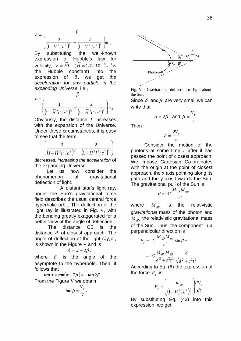
38

( ) ( ) 022222 12

1

32

3 i

i

mcVcV

Fa

⎟⎟

⎠

⎞

⎜⎜

⎝

⎛

−−

−

=r

r

By substituting the well-known expression of Hubble’s law for velocity, , ( is the Hubble constant) into the expression of , we get the acceleration for any particle in the expanding Universe, i.e.,

lHV ~= 1181071 −−×= sH .~

ar

( ) ( ) 02222222 ~1

2~1

32

3 i

i

mclHclH

Fa

⎟⎟

⎠

⎞

⎜⎜

⎝

⎛

−−

−

=

rr

Obviously, the distance l increases with the expansion of the Universe. Under these circumstances, it is easy to see that the term

( ) ( ) ⎟⎟

⎠

⎞

⎜⎜

⎝

⎛

−−

−2222222 ~1

2~1

32

3

clHclHdecreases, increasing the acceleration of the expanding Universe. Let us now consider the phenomenon of gravitational deflection of light. A distant star’s light ray, under the Sun’s gravitational force field describes the usual central force hyperbolic orbit. The deflection of the light ray is illustrated in Fig. V, with the bending greatly exaggerated for a better view of the angle of deflection. The distance CS is the distance of closest approach. The angle of deflection of the light ray,

dδ ,

is shown in the Figure V and is .βπδ 2−=

where β is the angle of the asymptote to the hyperbole. Then, it follows that

( ) ββπδ 22 tantantan −=−=From the Figure V we obtain

.tanc

Vy=β

δ Fig. V – Gravitational deflection of light about the Sun.

S C β β

Photons

Since δ and β are very small we can write that

βδ 2= and c

Vy=β

Then

cVy2

=δ

Consider the motion of the photons at some time after it has passed the point of closest approach. We impose Cartesian Co-ordinates with the origin at the point of closest approach, the x axis pointing along its path and the y axis towards the Sun. The gravitational pull of the Sun is

t

2r

MMGP gpgS−=

where is the relativistic gravitational mass of the photon and

the relativistic gravitational mass of the Sun. Thus, the component in a perpendicular direction is

gpM

gSM

222222

2 sin

tcd

dtcd

MMG

r

MMGF

gpgS

gpgSy

++−=

=−= β

According to Eq. (6) the expression of the force is yF

( ) dtdV

cV

mF y

y

gpy ⎟⎟

⎟

⎠

⎞

⎜⎜⎜

⎝

⎛

−=

23

221By substituting Eq. (43) into this expression, we get

39

( ) ( ) dtdV

McVcV

F yip

yyy ⎟⎟

⎟

⎠

⎞

⎜⎜⎜

⎝

⎛

−−

−=

23

22221

21

3

For , we can write this expression in the following form

cVy <<

( )dtdVMF yipy = . This force acts on the photons for a time causing an increase in the transverse velocity

t

dtMF

dVip

yy =

Thus the component of transverse velocity acquired after passing the point of closest approach is

( )( )

⎟⎟⎠

⎞⎜⎜⎝

⎛−=⎟

⎟⎠

⎞⎜⎜⎝

⎛−=

=+

−= ∫

ip

gpgS

ip

gpgS

gS

ip

gpy

mm

dcGM

MM

dcGM

dttcd

GMdMM

V23

222

Since the angle of deflection δ is given by

cVy2

2 == βδ

we readily obtain

⎟⎟⎠

⎞⎜⎜⎝

⎛−==

ip

gpgSy

mm

dc

GMcV

2

22δ

If 2=ipgp mm , the expression above gives

dc

GM gS2

4−=δ

As we know, this is the correct formula indicated by the experimental results. Equation (4) says that

ipip

gp mcm

pm⎪⎭

⎪⎬

⎫

⎪⎩

⎪⎨

⎧

⎥⎥⎥

⎦

⎤

⎢⎢⎢

⎣

⎡−⎟

⎟⎠

⎞⎜⎜⎝

⎛ Δ+−= 1121

2

Since 2=ipgp mm then, by making λhp =Δ into the equation above we

get

ichfmip ⎟

⎠

⎞⎜⎝

⎛+= 232

Due to 2=ipgp mm we get

ichfmgp ⎟

⎠

⎞⎜⎝

⎛+= 234

This means that the gravitational and inertial masses of the photon are imaginaries, and invariants with respect to speed of photon, i.e.

ipip mM = and .On the other hand, we can write that

gpgp mM =

( ) ( ) ichfmmm imaginaryiprealipip ⎟

⎠

⎞⎜⎝

⎛=+= 232

and

( ) ( ) ichfmmm imaginarygprealgpgp ⎟

⎠⎞

⎜⎝⎛=+= 23

4

This means that we must have ( ) ( ) 0== realgprealip mm

The phenomenon of gravitational deflection of light about the Sun shows that the gravitational interaction between the Sun and the photons is attractive. Thus, due to the gravitational force between the Sun and a photon can be expressed by

( ) ( )2rmMGF imaginarygpSung−= , where

) is a quantity positive and imaginary, we conclude that the force

(imaginarygpm

F will only be attractive if the matter ( ) has negative imaginary gravitational mass.

(SungM )

The Eq. (41) shows that if the inertial mass of a particle is null then its gravitational mass is given by

cpmg Δ±= 2 where pΔ is the momentum variation due to the energy absorbed by the particle. If the energy of the particle is invariant, then 0=Δp and, consequently, its gravitational mass will also be null. This is the case of the photons, i.e., they have an invariant energy and a momentum hf

λh . As they cannot absorb additional energy, the variation in the momentum will be null ( )0=Δp and, therefore, their gravitational masses will also be null. However, if the energy of the particle is not invariant (it is able to absorb energy) then the absorbed energy will transfer the amount of motion

40

(momentum) to the particle, and consequently its gravitational mass will be increased. This means that the motion generates gravitational mass. On the other hand, if the gravitational mass of a particle is null then its inertial mass, according to Eq. (41), will be given by

cpmi

Δ±=

52

From Eqs. (4) and (7) we get

VcpV

cE

p g Δ⎟⎠⎞

⎜⎝⎛=Δ⎟⎟

⎠

⎞⎜⎜⎝

⎛=Δ 0

2

Thus we have

Vcp

mg Δ⎟⎠

⎞⎜⎝

⎛±=

202

and Vcp

mi Δ⎟⎟⎠

⎞⎜⎜⎝

⎛±=

20

52

Note that, like the gravitational mass, the inertial mass is also directly related to the motion, i.e., it is also generated by the motion. Thus, we can conclude that is the motion, or rather, the velocity is what makes the two types of mass. In this picture, the fundamental particles can be considered as immaterial vortex of velocity; it is the velocity of these vortexes that causes the fundamental particles to have masses. That is, there exists not matter in the usual sense; but just motion. Thus, the difference between matter and energy just consists of the diversity of the motion direction; rotating, closed in itself, in the matter; ondulatory, with open cycle, in the energy (See Fig. VI). Under this context, the Higgs mechanism† appears as a process, by which the velocity of an immaterial vortex can be increased or decreased by

imaginaryip

)

† The Standard Model is the name given to the current theory of fundamental particles and how they interact. This theory includes: Strong interaction and a combined theory of weak and electromagnetic interaction, known as electroweak theory. One part of the Standard Model is not yet well established. What causes the fundamental particles to have masses? The simplest idea is called the Higgs mechanism. This mechanism involves one additional particle, called the Higgs boson, and one additional force type, mediated by exchanges of this boson.

making the vortex (particle) gain or lose mass. If real motion is what makes real mass then, by analogy, we can say that imaginary mass is made by imaginary motion. This is not only a simple generalization of the process based on the theory of the imaginary functions, but also a fundamental conclusion related to the concept of imaginary mass that, as it will be shown, provides a coherent explanation for the materialization of the fundamental particles, in the beginning of the Universe. It is known that the simultaneous disappearance of a pair (electron/positron) liberates an amount of energy, , under the form of two photons with frequency , in such a way that

( )2

02 cm realei

f

( ) hfcm realei 22 20 =

Since the photon has imaginary masses associated to it, the phenomenon of transformation of the energy into suggests that the imaginary

energy of the photon, m , comes from the transformation of imaginary energy of the electron,

, just as the real energy of the photon, , results from the transformation of real energy of the electron, i.e.,

( )2

02 cm realei

hf2

( )2c

(2

0 cm imaginaryei

hf

( ) ( )

( ) hfcm

cmcm

imaginarypi

realeiimaginaryei

22

222

0

20

20

+=

=+

Then, it follows that

( ) ( )imaginaryipimaginaryei mm −=0 The sign (-) in the equation above, is due to the imaginary mass of the photon to be positive, on the contrary of the imaginary gravitational mass of the matter, which is negative, as we have already seen.

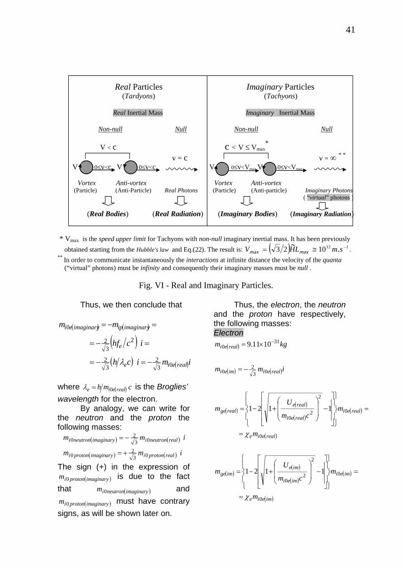
41

Real Particles Imaginary Particles (Tardyons) (Tachyons)

Real Inertial Mass Imaginary Inertial Mass

Non-null Null Non-null Null V < c c < V ≤ Vmax

* v = c v = ∞ * * V 0≤v<c V 0≤v<c V 0≤v<Vmax V 0≤v<Vmax Vortex Anti-vortex Vortex Anti-vortex (Particle) (Anti-Particle) Real Photons (Particle) (Anti-particle) Imaginary Photons ( “virtual” photons )

(Real Bodies) (Real Radiation) (Imaginary Bodies) (Imaginary Radiation) * Vmax is the speed upper limit for Tachyons with non-null imaginary inertial mass. It has been previously obtained starting from the Hubble's law and Eq.(22). The result is: ( ) 1121023 −≅= smLHV .~

maxmax . ** In order to communicate instantaneously the interactions at infinite distance the velocity of the quanta (“virtual” photons) must be infinity and consequently their imaginary masses must be null .

Fig. VI - Real and Imaginary Particles.

Thus, we then conclude that

( ) ( )

( )( ) ( )imich

ichf

mm

realeie

e

imaginaryipimaginaryei

032

32

23

2

0

−=−=

=−=

=−=

λ

where ( ) cmh realeie 0=λ is the Broglies’ wavelength for the electron. By analogy, we can write for the neutron and the proton the following masses:

( ) ( )

( ) ( ) imm

imm

realprotoniimaginaryprotoni

realneutroniimaginaryneutroni

032

0

032

0

+=

−=

The sign (+) in the expression of is due to the fact

that and must have contrary

signs, as will be shown later on.

(imaginaryprotonim 0

Thus, the electron, the neutron and the proton have respectively, the following masses: Electron

( )

( ) ( )

( )( )

( )( )

( )

( )( )

( )( )

( )imeie

imeiimei

imeimge

realeie

realeirealei

realerealge

realeiimei

realei

m

mcm

Um

m

mcm

Um

imm

kgm

0

0

2

20

0

0

2

20

032

0

310

1121

1121

1011.9

χ

χ

=

=⎪⎭

⎪⎬

⎫

⎪⎩

⎪⎨

⎧

⎥⎥⎥

⎦

⎤

⎢⎢⎢

⎣

⎡

−⎟⎟

⎠

⎞

⎜⎜

⎝

⎛+−=

=

=⎪⎭

⎪⎬

⎫

⎪⎩

⎪⎨

⎧

⎥⎥⎥

⎦

⎤

⎢⎢⎢

⎣

⎡

−⎟⎟

⎠

⎞

⎜⎜

⎝

⎛+−=

−=

×= −

)

)

)

(imaginaryneutronim 0

(imaginaryprotonim 0

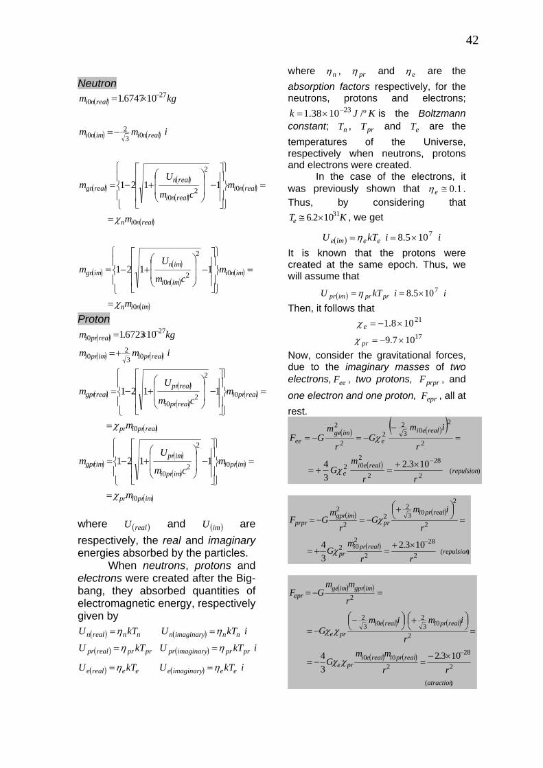
42

Neutron

( )

( ) ( )

( )( )

( )( )

( )

( )( )

( )( )

( )imnin

imniimni

imnimgn

realnin

realnirealni

realnrealgn

realniimni

realni

m

mcm

Um

m

mcm

Um

imm

kgm

0

0

2

20

0

0

2

20

032

0

270

1121

1121

106747.1

χ

χ

=

=⎪⎭

⎪⎬

⎫

⎪⎩

⎪⎨

⎧

⎥⎥⎥

⎦

⎤

⎢⎢⎢

⎣

⎡

−⎟⎟

⎠

⎞

⎜⎜

⎝

⎛+−=

=

=⎪⎭

⎪⎬

⎫

⎪⎩

⎪⎨

⎧

⎥⎥⎥

⎦

⎤

⎢⎢⎢

⎣

⎡

−⎟⎟

⎠

⎞

⎜⎜

⎝

⎛+−=

−=

×= −

Proton ( )

( ) ( )

( )( )

( )( )

( )

( )( )

( )( )

( )impripr

impriimpri

imprimgpr

realpripr

realprirealpri

realprrealgpr

realpriimpri

realpri

m

mcm

Um

m

mcm

Um

imm

kgm

0

0

2

20

0

0

2

20

032

0

270

1121

1121

106723.1

χ

χ

=

=⎪⎭

⎪⎬

⎫

⎪⎩

⎪⎨

⎧

⎥⎥⎥

⎦

⎤

⎢⎢⎢

⎣

⎡

−⎟⎟

⎠

⎞

⎜⎜

⎝

⎛+−=

=

=⎪⎭

⎪⎬

⎫

⎪⎩

⎪⎨

⎧

⎥⎥⎥

⎦

⎤

⎢⎢⎢

⎣

⎡

−⎟⎟

⎠

⎞

⎜⎜

⎝

⎛+−=

+=

×= −

)

where and are respectively, the real and imaginary energies absorbed by the particles.

(realU ( )imU

When neutrons, protons and electrons were created after the Big-bang, they absorbed quantities of electromagnetic energy, respectively given by

( ) ( )

( ) ( )

( ) ( ) ikTUkTU

ikTUkTU

ikTUkTU

eeimaginaryeeereale

prprimaginaryprprprrealpr

nnimaginarynnnrealn

ηη

ηη

ηη

==

==

==

where nη , prη and eη are the absorption factors respectively, for the neutrons, protons and electrons;

is the Boltzmann constant; , and are the temperatures of the Universe, respectively when neutrons, protons and electrons were created.

KJk /º1038.1 23−×=nT prT eT

In the case of the electrons, it was previously shown that 1.0≅eη . Thus, by considering that

, we get KTe31102.6 ×≅

( ) iikTU eeime7105.8 ×==η

It is known that the protons were created at the same epoch. Thus, we will assume that

( ) iikTU prprimpr7105.8 ×==η

Then, it follows that 21108.1 ×−=eχ17107.9 ×−=prχ

Now, consider the gravitational forces, due to the imaginary masses of two electrons, , two protons, , and one electron and one proton, , all at rest.

eeF prprF

eprF

( ) ( )( )

( ))(

2

28

2

202

2

203

22

2

2

103.234

repulsionrealei

e

realeie

imgeee

rr

mG

r

imG

r

mGF

−×+=+=

=−

−=−=

χ

χ

( ) ( )

( ))(2

28

2

202

2

2

032

22

2

103.234

repulsionrealpri

pr

realpripr

imgprprpr

rr

mG

r

imG

r

mGF

−×+=+=

=⎟⎠⎞⎜

⎝⎛+

−=−=

χ

χ

( ) ( )

( ) ( )

( ) ( )

)(

2

28

200

2

032

032

2

103.234

atraction

realprirealeipre

realprirealeipre

imgprimgeepr

rr

mmG

r

imimG

r

mmGF

−×−=−=

=⎟⎠⎞⎜

⎝⎛+⎟

⎠⎞⎜

⎝⎛−

−=

=−=

χχ

χχ

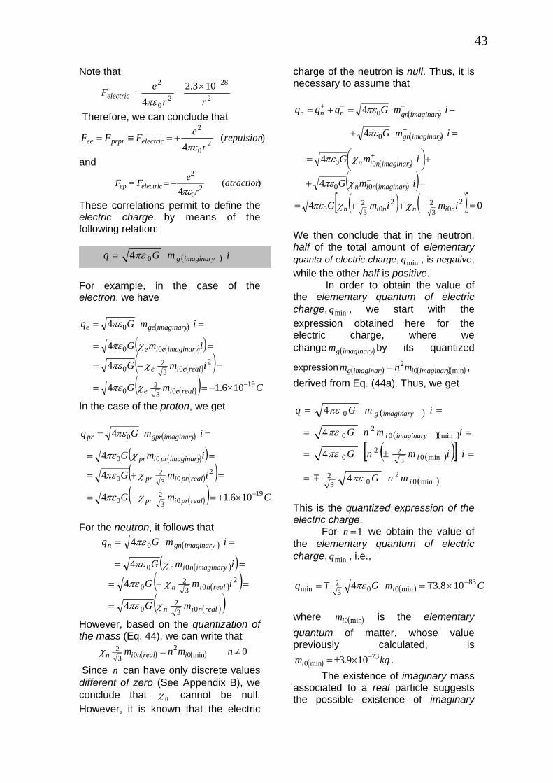
43

Note that

2

28

20

2 103.24 rr

eFelectric

−×==

πε Therefore, we can conclude that

)(4 2

0

2repulsion

reFFF electricprpree

πε+=≡=

and

)(4 2

0

2atraction

reFF electricep πε

−=≡

These correlations permit to define the electric charge by means of the following relation:

( ) imGq imaginaryg04πε=

For example, in the case of the electron, we have

( )

( )( )( )( )

( )( ) CmG

imG

imG

imGq

realeie

realeie

imaginaryeie

imaginarygee

1903

20

203

20

00

0

106.14

4

4

4

−×−==

=−=

==

==

χπε

χπε

χπε

πε

In the case of the proton, we get

( )

( )( )( )( )( )( ) CmG

imG

imG

imGq

realpripr

realpripr

imaginarypripr

imaginarygprpr

1903

20

203

20

00

0

106.14

4

4

4

−×+=−=

=+=

==

==

χπε

χπε

χπε

πε

For the neutron, it follows that

( )

( )( )( )( )

( )( )realnin

realnin

imaginarynin

imaginarygnn

mG

imG

imG

imGq

032

0

203

20

00

0

4

4

4

4

χπε

χπε

χπε

πε

=

=−=

==

==

However, based on the quantization of the mass (Eq. 44), we can write that

( ) ( ) 0min02

032 ≠= nmnm irealninχ

Since can have only discrete values different of zero (See Appendix B), we conclude that

n

nχ cannot be null. However, it is known that the electric

charge of the neutron is null. Thus, it is necessary to assume that

( )

( )

( )

( )( )( ) ( )[ ] 04

4

4

4

4

203

2203

20

00

00

0

0

=−++=

=+

+⎟⎠⎞⎜

⎝⎛=

=+

+=+=

−

+

−

+−+

imimG

imG

imG

imG

imGqqq

ninnin

imaginarynin

imaginarynin

imaginarygn

imaginarygnnnn

χχπε

χπε

χπε

πε

πε

We then conclude that in the neutron, half of the total amount of elementary quanta of electric charge, , is negative, while the other half is positive.

minq

In order to obtain the value of the elementary quantum of electric charge, , we start with the expression obtained here for the electric charge, where we change by its quantized

expression ,derived from Eq. (44a). Thus, we get

minq

(imaginarygm )

)( ) ( )(min02

imaginaryiimaginaryg mnm =

( )

( )( )

( )( )[ ]( )min0

203

2

min0322

0

min02

0

0

4

4

4

4

i

i

imaginaryi

imaginaryg

mnG

iimnG

imnG

imGq

πε

πε

πε

πε

m=

=±=

==

==

This is the quantized expression of the electric charge. For 1=n we obtain the value of the elementary quantum of electric charge, , i.e., minq

( ) CmGq i83

min0032

min 108.34 −×== mm πε

where is the elementary quantum of matter, whose value previously calculated, is

.

(min0im )

( ) kgmi73

min0 109.3 −×±=

The existence of imaginary mass associated to a real particle suggests the possible existence of imaginary

44

particles with imaginary masses in Nature. In this case, the concept of wave associated to a particle (De Broglie’s waves) would also be applied to the imaginary particles. Then, by analogy, the imaginary wave associated to an imaginary particle with imaginary masses and would be described by the following expressions

ψim ψgm

ψψ

ψψ

ωh

rh

r

=

=

E

kp

Henceforth, for the sake of simplicity, we will use the Greek letterψ to stand for the word imaginary; is the momentum carried by the

ψpr

ψ wave and

its energy; ψE ψψ λπ2=kr

is the

propagation number and ψλ the

wavelength of the ψ wave; ψψ πω f2= is the cyclical frequency. According to Eq. (4), the momentum is ψpr

VMp g

rrψψ =

where is the velocity of the V ψ particle. By comparing the expressions of

we get ψpr

VMh

gψψλ =

It is known that the variable quantity which characterizes the De Broglie’s waves is called wave function, usually indicated by symbol . The wave function associated with a material particle describes the dynamic state of the particle: its value at a particular point x, y, z, t is related to the probability of finding the particle in that place and instant. Although does not have a physical interpretation, its square (or

Ψ

Ψ

2Ψ Ψ *Ψ ) calculated for a particular point x, y, z, t is proportional to the probability of finding the particle in that place and instant. Since is proportional to the probability of finding the particle described by Ψ , the integral of

2ΨP

2Ψ on

the whole space must be finite − inasmuch as the particle is somewhere. On the other hand, if

02 =Ψ∫+∞

∞−Vd

the interpretation is that the particle will not exist. However, if

( )1082 ∞=Ψ∫+∞

∞−Vd

The particle will be everywhere simultaneously. In Quantum Mechanics, the wave function Ψ corresponds, as we know, to the displacement y of the undulatory motion of a rope. However, Ψ , as opposed to y , is not a measurable quantity and can, hence, be a complex quantity. For this reason, it is assumed that Ψ is described in the

directionx − by ( )( )pxEthie −−Ψ=Ψ π2

0

This is the expression of the wave function for a free particle, with total energy E and momentum , moving in the direction

pr

x+ . As to the imaginary particle, the imaginary particle wave function will be denoted by ψΨ and, by analogy the expression of Ψ , will be expressed by:

( )( )xptEhie ψψπψψ

−−Ψ=Ψ 20

Therefore, the general expression of the wave function for a free particle can be written in the following form

( )( ) ( ) ( )( )

( )( )xptEhi

xptEhireal

e

e realreal

ψψπψ

π

−−

−−

Ψ+

+Ψ=Ψ2

0

20

It is known that the uncertainty principle can also be written as a function of EΔ (uncertainty in the energy) and tΔ (uncertainty in the time), i.e.,

h≥ΔΔ tE. This expression shows that a variation of energy EΔ , during a

45

time interval , can only be detected if

tΔEt Δ≥Δ h . Consequently,

a variation of energy EΔ , during a time interval Et Δ<Δ h , cannot be experimentally detected. This is a limitation imposed by Nature and not by our equipments. Thus, a quantum of energy

that varies during a time interval

hfE =ΔEcft Δ<==Δ hλ1 (wave

period) cannot be experimentally detected. This is an imaginary photon or a “virtual” photon. Now, consider a particle with energy . The DeBroglie’s gravitational and inertial wavelengths are respectively

2cM g

cMh gg =λ and cMh ii =λ . In Quantum Mechanics,

particles of matter and quanta of radiation are described by means of wave packet (DeBroglie’s waves) with average wavelength iλ . Therefore, we can say that during a time interval ct iλ=Δ , a quantum of energy varies. According to the uncertainty principle, the particle will be detected if

2cME g=Δ

Et Δ≥Δ h , i.e., if 2cMc gi h≥λ or πλλ 2gi ≥ . This condition is usually satisfied when . In this case, ig MM = ig λλ = and obviously, πλλ 2ii > . However, when decreases gM gλ increases and πλ 2g can become bigger than

iλ , making the particle non-detectable or imaginary. According to Eqs. (7) and (41) we can write in the following form:

gM

iig

g McV

m

cV

mM χ

χ=

−=

−=

2222 11

where

( )⎭⎬⎫

⎩⎨⎧

⎥⎦⎤

⎢⎣⎡ −Δ+−= 1121 2

0cmp iχ

Since the condition to make the particle imaginary is

πλ

λ2

gi <

and

πχλ

χπλ

22i

ig

g

cMcM===

hh

Then we get

159.021

=<π

χ

However, χ can be positive or negative ( 159.0+<χ or 159.0−>χ ).This means that when

15901590 .. +<<− χ the particle becomes imaginary. Under these circumstances, we can say that the particle made a transition to the imaginary space-time. Note that, when a particle becomes imaginary, its gravitational and inertial masses also become imaginary. However, the factor

( ) ( )imaginaryiimaginaryg MM=χ remains real because

( )

( )real

MM

iMiM

MM

i

g

i

g

imaginaryi

imaginaryg ====χ

46

χ +0.159 ∞≤≤ V0 Imaginary Body 0 Imaginary Space-time “Virtual” Photons ( ∞=V ) −0.159 Fig. VII – Travel in the imaginary space-time. Similarly to the “virtual” photons, imaginary bodies can have infinite speed in the imaginary space-time.

Ordinary Space-time cV <≤0

Body

Ordinary Space-time

Real Photons ( cV = )

47

Real particle Real particle Δt1 ΔE

Δt2 c (speed upper limit)

Δt3

Imaginary Space-time Ordinary Space-time

Δt3

Δt2 Vmax

(speed upper limit)

ΔE Δt1

Imaginary particle Imaginary particle Fig. VIII – “Virtual” Transitions – (a) “Virtual” Transitions of a real particle to the imaginary space-time. The speed upper limit for real particle in the imaginary space-time is c. (b) - “Virtual” Transitions of an imaginary particle to the ordinary space-time. The speed upper limit for imaginary particle in the ordinary space-time is 11210 −≈ smV .max

Note that to occur a “virtual” transition it is necessary thatΔt=Δt1+ Δt2+ Δt3 <ℏ/ΔE Thus, even at principle, it will be impossible to determine any variation of energy in the particle (uncertainty principle).

(a)

(b)

48

Thus, if the gravitational mass of the particle is reduced by means of the absorption of an amount of electromagnetic energy U , for example, we have

( )⎭⎬⎫

⎩⎨⎧

⎥⎦⎤

⎢⎣⎡ −+−== 1121

220cmU

MM

ii

gχ

This shows that the energyU of the electromagnetic field remains acting on the imaginary particle. In practice, this means that electromagnetic fields act on imaginary particles. The gravity acceleration on a imaginary particle (due to the rest of the imaginary Universe) are given by

.,...,,, njgg jj 321==′ χ where ( ) ( )imaginaryiimaginaryg MM=χ

and ( )2jimaginarygjj rGmg −= . Thus,

the gravitational forces acting on the particle are given by

( )

( ) ( )( )( ) .22

2

jgjgjgjg

jimaginarygjimaginaryg

jimaginaryggj

rmGMriGmiM

rGmM

gMF

χχ

χ

+=−=

=−=

=′=

Note that these forces are real. Remind that, the Mach’s principle says that the inertial effects upon a particle are consequence of the gravitational interaction of the particle with the rest of the Universe. Then we can conclude that the inertial forces upon an imaginary particle are also real. Equation (7) shows that , in the case of imaginary particles, the relativistic mass is

( )( )

11

1

2222

22

−=

−=

=−

=

cV

im

cVi

imcV

mM

gg

imaginarygimaginaryg

This expression shows that imaginary particles can have velocities greater than in our ordinary space-time (Tachyons). The quantization of velocity (Eq. 36) shows that there is a speed upper limit . As we have already calculated previously, , (Eq.102).

V c

cV >max11210 −≈ smV .max

Note that this is the speed upper limit for imaginary particles in our ordinary space-time not in the imaginary space-time (Fig.7) because the infinite speed of the “virtual” quanta of the interactions shows that imaginary particles can have infinite speed in the imaginary space-time. While the speed upper limit for imaginary particles in the ordinary space-time is

, the speed upper limit for real particles in the imaginary space-time is c , because the relativistic expression of the mass shows that the velocity of real particles cannot be larger than c in any space-time. The uncertainty principle permits that particles make “virtual” transitions, during a time interval

11210 −≈ smV .max

tΔ , if Et Δ<Δ h . The “virtual” transition of mesons emitted from nucleons that do not change of mass, during a time interval

2cmt πh<Δ , is a well-known example of “virtual” transition of particles. During a “virtual” transition of a real particle, the speed upper limit in the imaginary space-time is c , while the speed upper limit for an imaginary particle

49

in the our ordinary space-time is . (See Fig. 8). 11210 −≈ smV .max

There is a crucial cosmological problem to be solved: the problem of the hidden mass. Most theories predict that the amount of known matter, detectable and available in the universe, is only about 1/100 to 1/10 of the amount needed to close the universe. That is, to achieve the density sufficient to close-up the universe by maintaining the gravitational curvature (escape velocity equal to the speed of light) at the outer boundary. Eq. (43) may solve this problem. We will start by substituting the expression of Hubble's law for velocity, lH~V = , into Eq.(43). The expression obtained shows that particles which are at distances

( )( ) m.H~cll 260 103135 ×=== have

quasi null gravitational mass ) ; beyond this distance,

the particles have negative gravitational mass. Therefore, there are two well-defined regions in the Universe; the region of the bodies with positive gravitational masses and the region of the bodies with negative gravitational mass. The total gravitational mass of the first region, in accordance with Eq.(45), will be given by

(mingg mm =

1221

111

1i

iig m

cVmMM ≅

−=≅

where is the total inertial mass of the bodies of the mentioned region;

1im

cV <<1 is the average velocity of the bodies at region 1. The total gravitational mass of the second region is

2222

2 11

121 ig McV

M ⎟⎟

⎠

⎞

⎜⎜

⎝

⎛−

−−=

where 2V is the average velocity

of the bodies ; 22

222 1 cVmM ii −= and is the total inertial mass of the bodies of region 2.

2im

Now consider that from Eq.(7), we can write

22

ccME

ggg ρξ ===VV

where ξ is the energy density of matter. Note that the expression of ξ only reduces to the well-known expression , where 2cρ ρ is the sum of the inertial masses per volume unit, when . Therefore, in the derivation of the well-known difference

ig mm =

2

38

HG U ~−

ρπ

which gives the sign of the curvature of the Universe [36], we must use

instead of .The result obviously is

2cgUρξ = 2cUρξ =

( )1093

8 2H~G gU −

ρπ

where

( )11021

U

gg

U

gUgU

MMMVV+

==ρ

gUM and UV are respectively the total gravitational mass and the volume of the Universe. Substitution of and into expression (110) gives

1gM 2gM

U

iiiU

gU

mmcVcV

m

V

⎥⎥

⎦

⎤

⎢⎢

⎣

⎡−

−−

−+

=

22222

222

12

1

3

ρ

where 21 iiiU mmm += is the total inertial mass of the Universe. The volume 1V of the region 1 and the volume 2V of the region 2, are respectively given by

50

132

230

21 22 VVV −== clandl ππ

where m.H~clc

261081 ×== is the so-called "radius" of the visible Universe. Moreover, 111 Vii m=ρ and

222 Vii m=ρ . Due to the hypothesis of the uniform distribution of matter in the space, it follows that

21 ii ρρ = .Thus, we can write

3803

0

2

1

2

1 .ll

mm

ci

i =⎟⎟⎠

⎞⎜⎜⎝

⎛==

VV

Similarly,

1

1

2

2

VVVii

U

iU mmm==

Therefore,

iUiUc

iUU

i m.mll

mm 62013

022 =

⎥⎥⎦

⎤

⎢⎢⎣

⎡⎟⎟⎠

⎞⎜⎜⎝

⎛−==

VV

and . iUi m.m 3801 =Substitution of into the expression of

2im

gUρ yields

U

iUiU

gU

mcVcV

m

V

6201

241

1

86122

222

2

...−

−−

−+

=ρ

Due to cV ≅2 , we conclude that the term between bracket is much larger than . The amount is the mass of matter in the universe (1/10 to 1/100 of the amount needed to close the Universe).

iUm10 iUm

Consequently, the total mass

iUiU mcVcV

m 6201

241

1

86122

222

2

...−

−−

−+

must be sufficient to close the Universe. There is another cosmological problem to be solved: the problem of

the anomalies in the spectral red-shift of certain galaxies and stars. Several observers have noticed red-shift values that cannot be explained by the Doppler-Fizeau effect or by the Einstein effect (the gravitational spectrum shift, supplied by Einstein's theory). This is the case of the so-called Stefan's quintet (a set of five galaxies which were discovered in 1877), whose galaxies are located at approximately the same distance from the Earth, according to very reliable and precise measuring methods. But, when the velocities of the galaxies are measured by its red-shifts, the velocity of one of them is much larger than the velocity of the others. Similar observations have been made on the Virgo constellation and spiral galaxies. Also the Sun presents a red-shift greater than the predicted value by the Einstein effect. It seems that some of these anomalies can be explained if we consider the Eq.(45) in the calculation of the gravitational mass of the point of emission. The expression of the gravitational spectrum shift was previously obtained in this work. It is the same supplied by Einstein's theory [37], and is given by

( )111021122

0212

21

ω

ωφ φωωω

c

rGmrGmc

gg +−=

=−

=−=Δ

where 1ω is the frequency of the light at the point of emission ; 2ω is the frequency at the point of observation; 1φ and 2φ are respectively, the Newtonian gravitational potentials at the point of emission and at the point of observation.

51

In Einstein theory, this expression has been deduced from

00gtT −= [38] which correlates own time (real time), t , with the temporal coordinate x0 of the space-time ( cxt 0= ). When the gravitational field is weak, the temporal component of the metric tensor is given by

2[

00g

21 c/goo φ−−= 39].Thus, we readily obtain

( )11221 2rcGmtT g−=

This is the same equation that we have obtained previously in this work. Curiously, this equation tell us that we can have when ; and for . In addition, if

tT < 0>gmtT > 0<gm

Grcmg 22= , i.e., if 22 cGmr g= (Schwarzschild radius) we obtain

0=T .

Let us now consider the well-known process of stars' gravitational contraction. It is known that the destination of the star is directly correlated to its mass. If the star's mass is less than 1.4M (Schemberg-Chandrasekhar's limit), it becomes a white dwarf. If its mass exceeds that limit, the pressure produced by the degenerate state of the matter no longer counterbalances the gravitational pressure, and the star's contraction continues. Afterwards there occurs the reactions between protons and electrons (capture of electrons), where neutrons and anti-neutrinos are produced.

The contraction continues until the system regains stability (when the pressure produced by the neutrons is sufficient to stop the gravitational collapse). Such systems are called neutron stars.

There is also a critical mass for the stable configuration of neutron stars. This limit has not

been fully defined as yet, but it is known that it is located between 1.8M and 2.4M . Thus, if the mass of the star exceeds 2.4M , the contraction will continue. According to Hawking [40] collapsed objects cannot have mass less than kg.Gc 810114 −×=h . This means that, with the progressing of the compression, the neutrons cluster must become a cluster of superparticles where the minimal inertial mass of the superparticle is

( ) ( )1131011 8 .kg.m spi−×=

Symmetry is a fundamental attribute of the Universe that enables an investigator to study particular aspects of physical systems by themselves. For example, the assumption that space is homogeneous and isotropic is based on Symmetry Principle. Also here, by symmetry, we can assume that there are only superparticles with mass in the cluster of superparticles.

( ) kg.m spi81011 −×=

Based on the mass-energy of the superparticles ( ~1018 GeV ) we can say that they belong to a putative class of particles with mass-energy beyond the supermassive Higgs bosons ( the so-called X bosons). It is known that the GUT's theories predict an entirely new force mediated by a new type of boson, called simply X (or X boson ). The X bosons carry both electromagnetic and color charge, in order to ensure proper conservation of those charges in any interactions. The X bosons must be extremely massive, with mass-energy in the unification range of about 1016 GeV. If we assume the superparticles are not hypermassive Higgs bosons then the possibility of the neutrons cluster become a

52

Higgs bosons cluster before becoming a superparticles cluster must be considered. On the other hand, the fact that superparticles must be so massive also means that it is not possible to create them in any conceivable particle accelerator that could be built. They can exist as free particles only at a very early stage of the Big Bang from which the universe emerged. Let us now imagine the Universe coming back to the past. There will be an instant in which it will be similar to a neutrons cluster, such as the stars at the final state of gravitational contraction. Thus, with the progressing of the compression, the neutrons cluster becomes a superparticles cluster. Obviously, this only can occur before 10-23s (after the Big-Bang). The temperature T of the Universe at the 10-43s< t < 10-23s period can be calculated by means of the well-known expression[41]:

( ) ( )1141010 212322 −−≈ tT

Thus at (at the first spontaneous breaking of symmetry) the temperature was (∼10

st 4310 −≅

KT 3210≈19GeV).Therefore, we can

assume that the absorbed electromagnetic energy by each superparticle, before , was

(see Eqs.(71) and (72)). By comparing with

, we conclude that . Therefore, the

unification condition

st 4310 −≅JkTU 9101×>=η

( ) Jcm spi82 109×≅

( )cmU spi>

( )22 cmcMUn iir >≅ is satisfied. This means that, before

,the gravitational and electromagnetic interactions were unified.

st 4310 −≅

From the unification condition ( )2cMUn ir ≅ , we may conclude that

the superparticles' relativistic inertial mass is ( )spiM

( ) ( )11510 822 kg

ckTn

cUn

M rrspi

−≈=≅η

Comparing with the superparticles' inertial mass at rest (113), we conclude that

( ) ( ) ( )1161011 8kg.mM spispi−×=≈

From Eqs.(83) and (115), we obtain the superparticle's gravitational mass at rest:

( ) ( ) ( )

( ) ( )117

2

2ckTn

M

Mmm

rspi

spispispg

η−≅−≅

≅−=

Consequently, the superparticle's relativistic gravitational mass, is

( )( )

( )1181

1

222

22

cVc

kTncV

mM

r

spgspg

−=

=−

=

η

Thus, the gravitational forces between two superparticles , according to (13), is given by:

( ) ( )

( )

( )( ) ( )119212

25

2

2122112

μκη

μ

ˆrcTn

cG

mM

ˆrMM

GFF

rspi

spi

'spgspg

h

h

rr

⎥⎥

⎦

⎤

⎢⎢

⎣

⎡⎟⎠⎞

⎜⎝⎛

⎟⎟⎠

⎞⎜⎜⎝

⎛=

=−=−=

Due to the unification of the gravitational and electromagnetic interactions at that period, we have

53

( ) ( )

( )

( )( )

( )1204 2

0

2

2122

5

2

2122112

re

ˆrcT

cG

mM

ˆrMM

GFF

spi

spi

'spgspg

πε

μηκ

μ

=

=⎥⎥

⎦

⎤

⎢⎢

⎣

⎡⎟⎠⎞

⎜⎝⎛

⎟⎟⎠

⎞⎜⎜⎝

⎛=

==−=

h

h

rr

From the equation above we can write

( )

( )( ) ( )121

4 0

22

5

2

πεηκ ecT

cG

mM

spi

spi =⎥⎥

⎦

⎤

⎢⎢

⎣

⎡⎟⎠⎞

⎜⎝⎛

⎟⎟⎠

⎞⎜⎜⎝

⎛h

h

Now assuming that

( )

( )( ) (1222

5

2

ψηκ =⎟⎠⎞

⎜⎝⎛

⎟⎟⎠

⎞⎜⎜⎝

⎛T

cG

mM

spi

spi

h)

the Eq. (121) can be rewritten in the following form:

( )123137

14 0

2

==c

ehπε

ψ

which is the well-known reciprocal fine structure constant. For the Eq.(122) gives

KT 3210=

( )

( )( ) ( )124

10012

5

2

≈⎟⎠⎞

⎜⎝⎛

⎟⎟⎠

⎞⎜⎜⎝

⎛= Tn

cG

mM

rspi

spi κηψh

This value has the same order of magnitude as the exact value(1/137) of the reciprocal fine structure constant. From equation (120) we can write:

( ) ( ) ( )125hr

r =⎟⎟⎠

⎞⎜⎜⎝

⎛r

rcMM

G'

spgspg

ψ

The term between parentheses has the same dimensions as the linear momentum . Thus, (125) tells us that

pr

( )126.rp hrr

=⋅A component of the momentum of a particle cannot be precisely specified without loss of all knowledge of the corresponding

component of its position at that time ,i.e., a particle cannot be precisely located in a particular direction without loss of all knowledge of its momentum component in that direction . This means that in intermediate cases the product of the uncertainties of the simultaneously measurable values of corresponding position and momentum components is at least of the magnitude order of , h

( )127h≥r.p ΔΔ This relation, directly obtained here from the Unified Theory, is the well-known relation of the Uncertainty Principle for position and momentum. According to Eq.(83), the gravitational mass of the superparticles at the center of the cluster becomes negative when

( )spir mckTn >22η , i.e., when

( ) .102

322

Kkn

cmTT

r

spicritical ≈=>

η According to Eq. (114) this temperature corresponds to . With the progressing of the compression, more superparticles into the center will have negative gravitational mass. Consequently, there will be a critical point in which the repulsive gravitational forces between the superparticles with negative gravitational masses and the superparticles with positive gravitational masses will be so strong that an explosion will occur. This is the event that we call the Big Bang.

stc4310−≈

Now, starting from the Big Bang to the present time. Immediately after the Big Bang, the superparticles' decompression

54

begins. The gravitational mass of the most central superparticle will only be positive when the temperature becomes smaller than the critical temperature, . At the maximum state of compression (exactly at the Big Bang) the volumes of the superparticles were equal to the elementary volume and the volume of the Universe was

where was the initial length scale of the Universe. At this very moment the average density of the Universe was equal to the average density of the superparticles, thus we can write

KTcritical3210≈

30 mindVδ=Ω

( ) 33initialVminV dnd δδΩ == initiald

( )

( )( )128

3

spi

Ui

min

initial

mM

dd

=⎟⎟⎠

⎞⎜⎜⎝

⎛

where is the inertial mass of the Universe. It has already been shown that

( ) kgM Ui5310≈

.mlk~d planckmin3410−≈= Then, from

Eq.(128), we obtain:

( )12910 14mdinitial−≈

After the Big Bang the Universe expands itself from up to (when the temperature decrease reaches the critical temperature , and the gravity becomes attractive). Thus, it expands by , under effect of the repulsive gravity

initiald

crd

KTcritical3210≈

initialcr dd −

( )( ) ( )[ ] ( ) ( )[

during a period of time .Thus,

stc4310−≈

( ) ( ) ( ) ( ) ( )1302221

cinitialcr

Uicinitialcr t

ddGM

tgdd χ==−

The Eq.(83), gives

( )

( ) ( ) ( )22

21

21

cmkTn

cmUn

m

m

spi

r

spi

r

spi

spg ηχ −=−==

Calculations by Carr, B.J [41], indicate that it would seem reasonable to suppose that the fraction of initial primordial black hole mass ultimately converted into photons is about . This means that we can take

11.0

11.0=η

Thus, the amount , where is the total inertial mass of the Universe, expresses the total amount of inertial energy converted into photons at the initial instant of the Universe(Primordial Photons).

2cMiUη

iUM

It was previously shown that photons and also the matter have imaginary gravitational masses associated to them. The matter has negative imaginary gravitational mass, while the photons have positive imaginary gravitational mass, given by

( ) ( ) ichfMM imaginaryipimaginarygp ⎟

⎠

⎞⎜⎝

⎛+== 2342

]( ) ( ) ( ) ( )

( ) ( ) ( )

initialcr

Ui

initialcr

Uispi

initialcr

Uispg

initialcr

UiUg

crUiinitialUg

minmax

ddGM

ddMmG

ddMmG

ddMMG

dMGdMG

ggg

χχ 22

22

221

212

21

21

==

===

==

==

∑

∑

where is the imaginary inertial mass of the photons.

)(imaginaryipM

Then, from the above we can conclude that, at the initial instant of the Universe, an amount of imaginary gravitational mass,

, which was associated to the fraction of the matter transformed into photons, has been converted into imaginary gravitational mass of the primordial

totalimaginarygmM )(

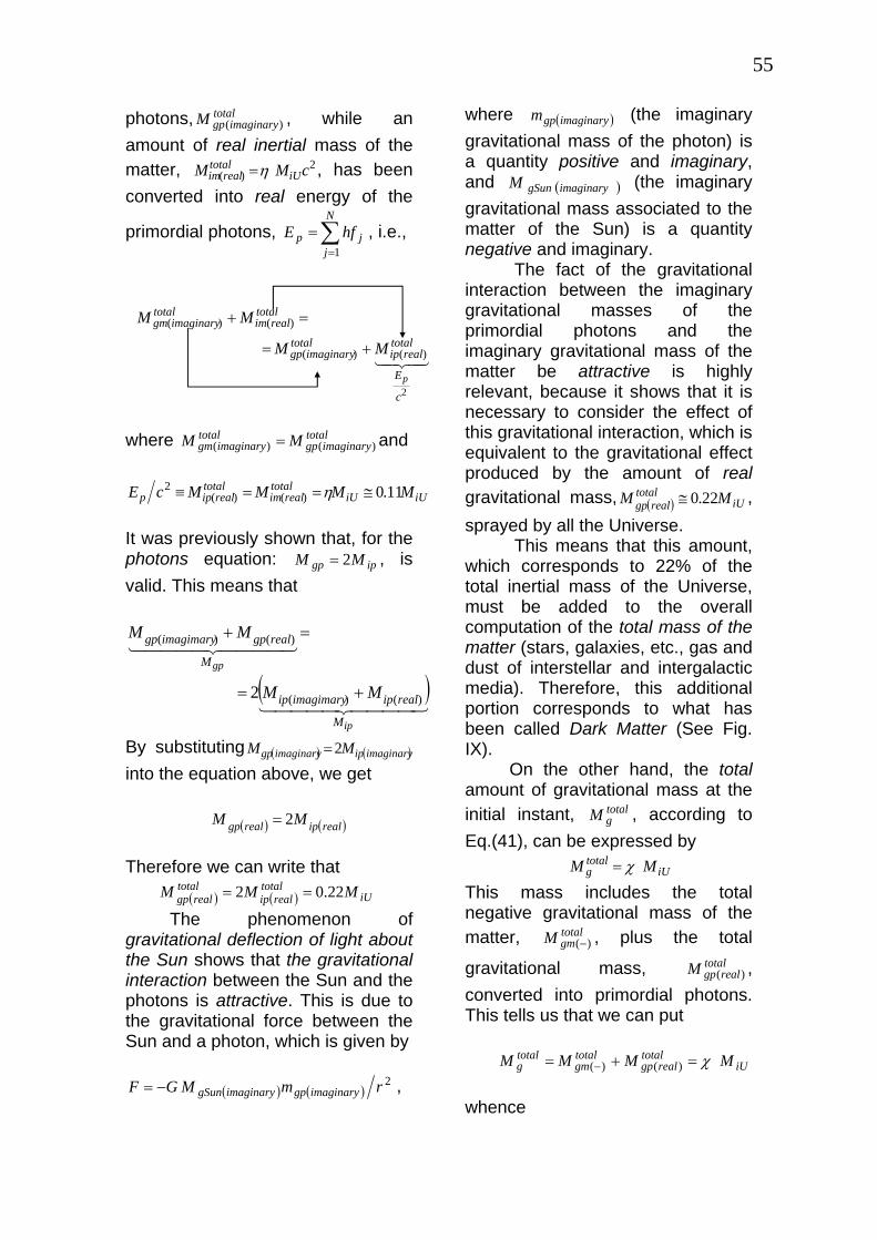
55

photons, , while an amount of real inertial mass of the matter, , has been converted into real energy of the

primordial photons, , i.e.,

totalimaginarygpM )(

2)( cMM iU

totalrealim η=

∑=

=N

jjp hfE

1

43421

2

)()(

)()(

c

E

totalrealip

totalimaginarygp

totalrealim

totalimaginarygm

p

MM

MM

+=

=+

where and total

imaginarygptotal

imaginarygm MM )()( =

iUiU

totalrealim

totalrealipp MMMMcE 11.0)()(

2 ≅==≡ η

It was previously shown that, for the photons equation: , is valid. This means that

ipgp MM 2=

(44444444 21

4444 34444 21

ip

gp

M

realipimagimaryip

M

realgpimagimarygp

MM

MM

)()(

)()(

2 +=

=+

)3

By substituting into the equation above, we get

( ) ( )imaginaryipimaginarygp MM 2=

( ) ( )realiprealgp MM 2=

Therefore we can write that

( ) ( ) iUtotal

realiptotal

realgp MMM 22.02 ==

The phenomenon of gravitational deflection of light about the Sun shows that the gravitational interaction between the Sun and the photons is attractive. This is due to the gravitational force between the Sun and a photon, which is given by

( ) ( )2rmMGF imaginarygpimaginarygSun−= ,

where (the imaginary gravitational mass of the photon) is a quantity positive and imaginary, and (the imaginary gravitational mass associated to the matter of the Sun) is a quantity negative and imaginary.

(imaginarygpm )

)(imaginarygSunM

The fact of the gravitational interaction between the imaginary gravitational masses of the primordial photons and the imaginary gravitational mass of the matter be attractive is highly relevant, because it shows that it is necessary to consider the effect of this gravitational interaction, which is equivalent to the gravitational effect produced by the amount of real gravitational mass, , sprayed by all the Universe.

( ) iUtotal

realgp MM 22.0≅

This means that this amount, which corresponds to 22% of the total inertial mass of the Universe, must be added to the overall computation of the total mass of the matter (stars, galaxies, etc., gas and dust of interstellar and intergalactic media). Therefore, this additional portion corresponds to what has been called Dark Matter (See Fig. IX). On the other hand, the total amount of gravitational mass at the initial instant, , according to Eq.(41), can be expressed by

totalgM

iUtotalg MM χ=

This mass includes the total negative gravitational mass of the matter, , plus the total

gravitational mass, , converted into primordial photons. This tells us that we can put

totalgmM )(−

totalrealgpM )(

iU

totalrealgp

totalgm

totalg MMMM χ=+= − )()(

whence

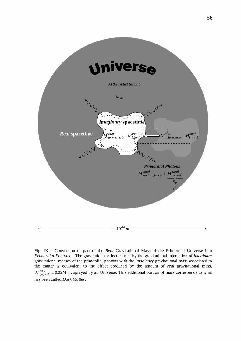
56

Fig. IX – Conversion of part of the Real Gravitational Mass of the Primordial Universe into Primordial Photons. The gravitational effect caused by the gravitational interaction of imaginarygravitational masses of the primordial photons with the imaginary gravitational mass associated to the matter is equivalent to the effect produced by the amount of real gravitational mass,

( ) iUtotal

realgp MM 22.0≅ , sprayed by all Universe. This additional portion of mass corresponds to what has been called Dark Matter.

∼ 10-14 m

Real spacetime

Imaginary spacetime

( ) ( )totalip

totalgp realimaginary MM + ( ) ( )

totalim

totalgm realimaginary MM +

At the Initial Instant

iUM

Primordial Photons

( ) ( )43421

2c

E

totalip

totalgp

p

realimaginary MM +

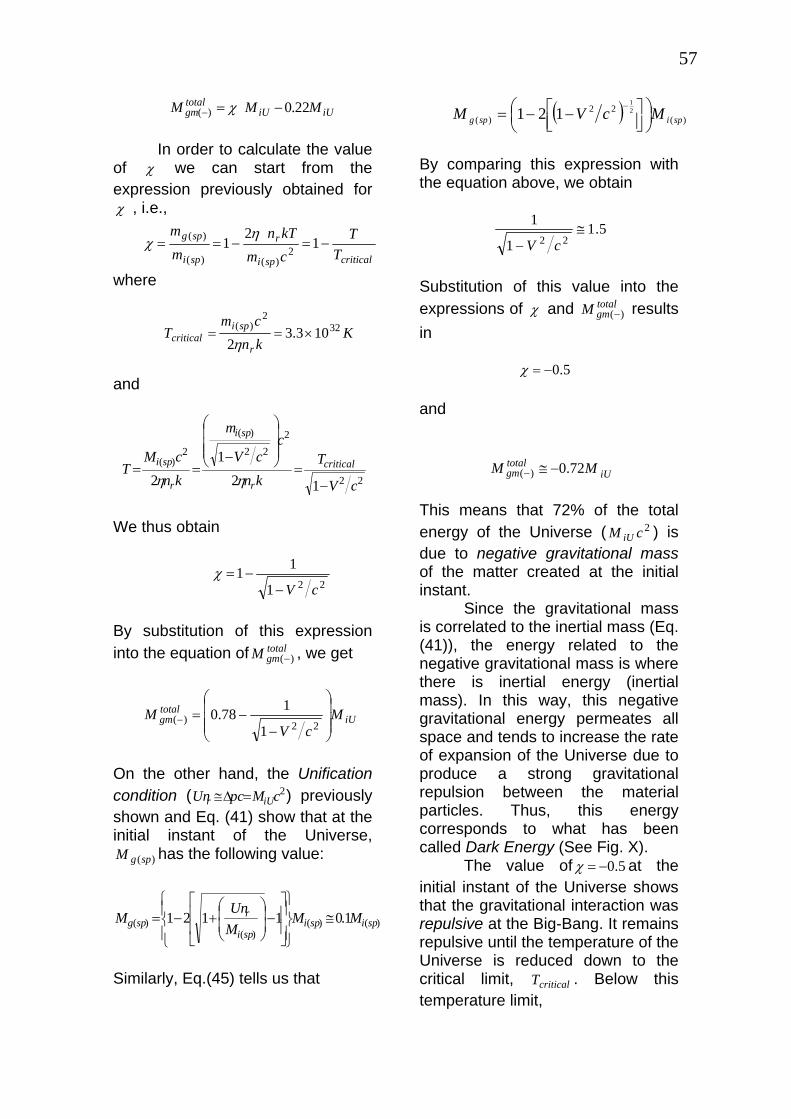
57

iUiUtotalgm MMM 22.0)( −=− χ

In order to calculate the value of χ we can start from the expression previously obtained for χ , i.e.,

criticalspi

r

spi

spg

TT

cmkTn

mm

−=−== 12

1 2)()(

)( ηχ

where

Kkncm

Tr

spicritical

322

)( 103.32

×==η

and

22

222

)(

2)(

121

2 cV

Tkn

ccV

m

kncM

T critical

r

spi

r

spi

−=

⎟⎟⎟

⎠

⎞

⎜⎜⎜

⎝

⎛

−==

ηη

We thus obtain

221

11cV−

−=χ

By substitution of this expression into the equation of , we get total

gmM )(−

iUtotalgm M

cVM

⎟⎟⎟

⎠

⎞

⎜⎜⎜

⎝

⎛

−−=− 22)(

1

178.0

On the other hand, the Unification condition ( ) previously shown and Eq. (41) show that at the initial instant of the Universe,

has the following value:

2cMpcUn iUr =Δ≅

)(spgM

)()()(

)( 1.01121 spispispi

rspg MM

MUn

M ≅⎪⎭

⎪⎬⎫

⎪⎩

⎪⎨⎧

⎥⎥

⎦

⎤

⎢⎢

⎣

⎡−⎟

⎟⎠

⎞⎜⎜⎝

⎛+−=

Similarly, Eq.(45) tells us that

( ) )(22

)(21

121 spispg McVM ⎟⎠⎞⎜

⎝⎛

⎥⎦⎤

⎢⎣⎡ −−=

−

By comparing this expression with the equation above, we obtain

5.11

122

≅− cV

Substitution of this value into the expressions of χ and results in

totalgmM )(−

5.0−=χ

and

iU

totalgm MM 72.0)( −≅−

This means that 72% of the total energy of the Universe ( ) is due to negative gravitational mass of the matter created at the initial instant.

2cM iU

Since the gravitational mass is correlated to the inertial mass (Eq. (41)), the energy related to the negative gravitational mass is where there is inertial energy (inertial mass). In this way, this negative gravitational energy permeates all space and tends to increase the rate of expansion of the Universe due to produce a strong gravitational repulsion between the material particles. Thus, this energy corresponds to what has been called Dark Energy (See Fig. X). The value of 5.0−=χ at the initial instant of the Universe shows that the gravitational interaction was repulsive at the Big-Bang. It remains repulsive until the temperature of the Universe is reduced down to the critical limit, . Below this temperature limit,

criticalT

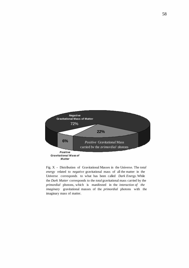
58

72%

6%

22%

Negative Gravitational Mass of Matter

PositiveGravitational M ass of

M atter

Fig. X - Distribution of Gravitational Masses in the Universe. The total energy related to negative gravitational mass of all the matter in the Universe corresponds to what has been called Dark Energy. While the Dark Matter corresponds to the total gravitational mass carried by the primordial photons, which is manifested in the interaction of the imaginary gravitational masses of the primordial photons with the imaginary mass of matter.

Positive Gravitational Mass carried by the primordial photons

59

the attractive component of the gravitational interaction became greater than the repulsive component, making attractive the resultant gravitational interaction. Therefore, at the beginning of the Universe – before the temperature decreased down to , there occurred an expansion of the Universe that was exponential in time rather than a normal power-law expansion. Thus, there was an evident Inflation Period during the beginning of the expansion of the Universe (See Fig. XI).

criticalT

With the progressing of the decompression the superparticles cluster becomes a neutrons cluster. This means that the neutrons are created without its antiparticle, the antineutron. Thus, this solves the matter/antimatter dilemma that is unresolved in many cosmologies. Now a question: How did the primordial superparticles appear at the beginning of the Universe? It is a proven quantum fact that a wave function may collapse, and that, at this moment, all the possibilities that it describes are suddenly expressed in reality. This means that, through this process, particles can be suddenly materialized. The materialization of the primordial superparticles into a critical volume denotes knowledge of what would happen with the Universe starting from that initial condition, a fact that points towards the existence of a Creator. It was shown previously the possible existence of imaginary particles with imaginary masses in Nature. These particles can be associated with real particles, such as in case of the photons and electrons, as we have shown, or they can be associated with others imaginary particles by constituting the

imaginary bodies. Just as the real particles constitute the real bodies. The idea that we make about a consciousness is basically that of an imaginary body containing psychic energy and intrinsic knowledge. We can relate psychic energy with psychic mass (psychic mass= psychic energy/c2). Thus, by analogy with the real bodies the psychic bodies would be constituted by psychic particles with psychic mass. Consequently, the psychic particles that constitute a consciousness would be equivalent to imaginary particles, and the psychic mass , ,of the psychic particles would be equivalent to the imaginary mass, i.e.,

Ψm

( ) ( )131imaginaryimm =Ψ

Thus, the imaginary masses associated to the photons and electrons would be elementary psyche actually, i.e.,

( )

( )1323

22 i

chf

mm photonimaginaryiphoton

⎟⎠

⎞⎜⎝

⎛=

==Ψ

( )

( ) ( )133032

232

im

ic

hf

mm

electronreali

electron

electronimaginaryielectron

−=

=⎟⎟⎠

⎞⎜⎜⎝

⎛−=

==Ψ

The idea that electrons have elementary psyche associated to themselves is not new. It comes from the pre-Socratic period. By proposing the existence of psyche associated with matter, we are adopting what is called panpsychic posture. Panpsychism dates back to the pre-Socratic period;

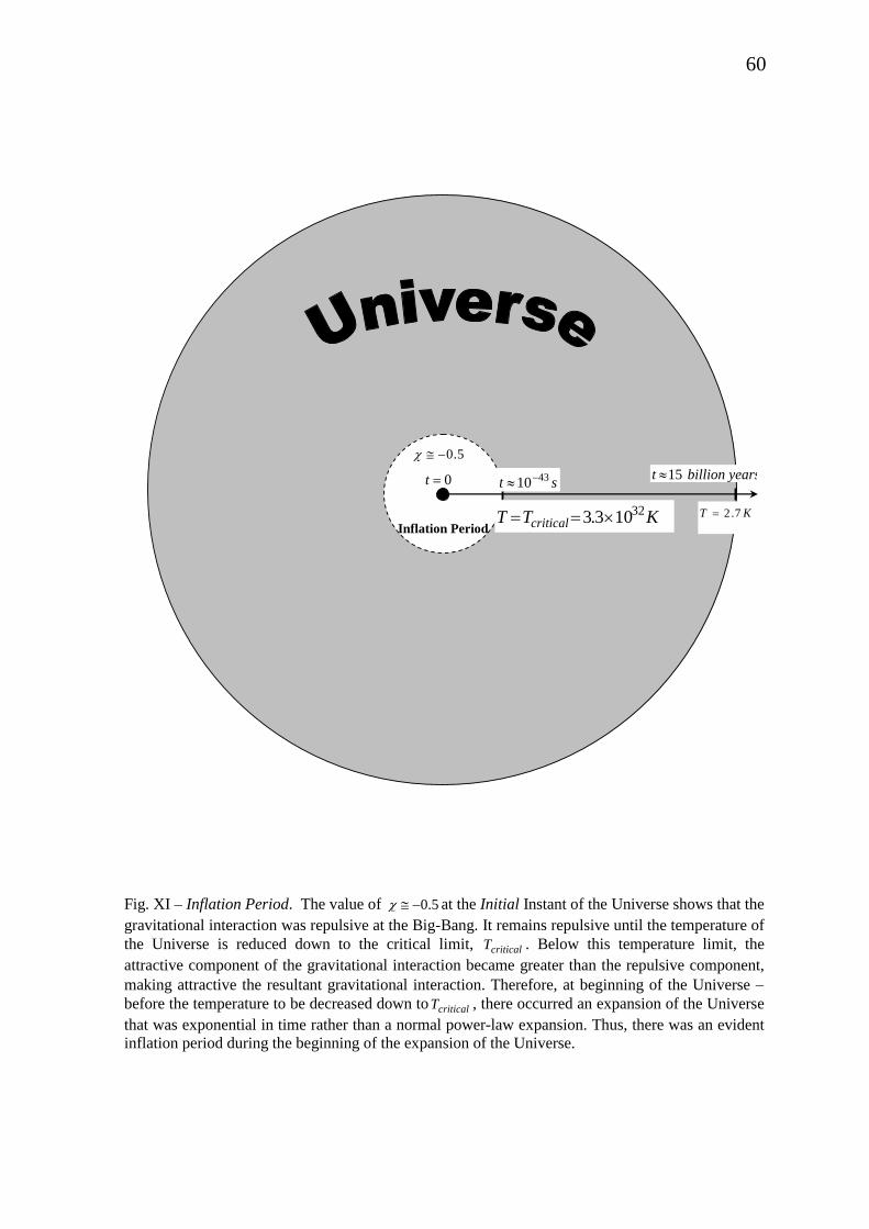
60

Fig. XI – Inflation Period. The value of 5.0−≅χ at the Initial Instant of the Universe shows that the gravitational interaction was repulsive at the Big-Bang. It remains repulsive until the temperature of the Universe is reduced down to the critical limit, criticalT . Below this temperature limit, the attractive component of the gravitational interaction became greater than the repulsive component, making attractive the resultant gravitational interaction. Therefore, at beginning of the Universe −before the temperature to be decreased down to criticalT , there occurred an expansion of the Universe that was exponential in time rather than a normal power-law expansion. Thus, there was an evident inflation period during the beginning of the expansion of the Universe.

0=t st 4310−≈

KTT critical32103.3 ×==

Inflation PeriodKT 7.2=

st 4310−≈ st 4310−≈ st 4310−≈ st 4310−≈ st 4310−≈ yearsbilliont 15≈

5.0−≅χ

61

remnants of organized panpsychism may be found in the Uno of Parmenides or in Heracleitus’s Divine Flow. The scholars of Miletus’s school were called hylozoists, that is, “those who believe that matter is alive”. More recently, we will find the panpsychistic thought in Spinoza, Whitehead and Teilhard de Chardin, among others. The latter one admitted the existence of proto-conscious properties at the elementary particles’ level. We can find experimental evidences of the existence of psyche associated to electron in an experiment similar to that commonly used to show the wave duality of light. (Fig. XII). One merely substitutes an electron ray (fine electron beam) for the light ray. Just as in the experiment mentioned above, the ray which goes through the holes is detected as a wave if a wave detector is used (it is then observed that the interference pattern left on the detector screen is analogous with that produced by the light ray), and as a particle if a particle detector is used. Since the electrons are detected on the other side of the metal sheet, it becomes obvious then that they passed through the holes. On the other hand, it is also evident that when they approached the holes, they had to decide which one of them to go through. How can an electron “decide” which hole to go through? Where there is “choice”, isn’t there also psyche, by definition? The existence of psyche mass associated to material particles can solve the black hole information

paradox ‡ if we assume that any information placed into a black hole is saved into the psyche mass associated to the black hole and after - during the evaporation of the black hole, carried by the psyche masses associated to the evaporated particles (Hawking radiation). Thus, if the material entering the black hole is a pure quantum state, the transformation of that state into the mixed state of Hawking radiation does not destroy information about the original quantum state because the psyche mass does not lose any structure of the original quantum state in the transformation. In this way, when information goes into a black hole it is not destroyed and might escape from the black hole during its evaporation. The idea of psyche mass associated to a black hole leads to conclusion that there has been a psyche mass associated to the Initial Universe.

‡ In 1975, Stephen Hawking showed that black holes eventually evaporate releasing particles containing no information (Hawking radiation). It was soon realized that this prediction created an information loss. From the no hair theorem one would expect the Hawking radiation to be completely independent of the material entering the black hole. However, if the material entering the black hole were a pure quantum state, the transformation of that state into the mixed state of Hawking radiation would destroy information about the original quantum state. This violates Liouville's theorem and presents a physical paradox. It is a contentious subject for science since it violated a commonly assumed tenet of science—that information cannot be destroyed.

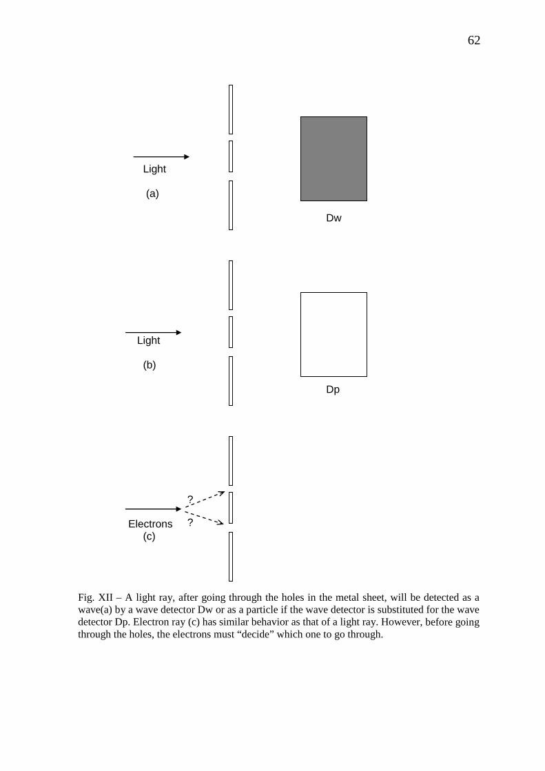
62

Light (a) Dw Light (b) Dp ? Electrons (c) Fig. XII – A light ray, after going through the holes in the metal sheet, will be detected as awave(a) by a wave detector Dw or as a particle if the wave detector is substituted for the wavedetector Dp. Electron ray (c) has similar behavior as that of a light ray. However, before going through the holes, the electrons must “decide” which one to go through.

?

63

If the primordial superparticles that have been materialized at the beginning of the Universe came from the collapse of a primordial wave function, then the psychic form described by this wave function must have been generated in a consciousness with a psychic mass much greater than that needed to materialize the Universe (material and psychic). This giant consciousness, in its turn, would not only be the greatest of all consciences in the Universe but also the substratum of everything that exists and, obviously, everything that exists would be entirely contained within it, including all the spacetime. Thus, if the consciousness we refer to contains all the space, its volume is necessarily infinite, consequently having an infinite psychic mass. This means that it contains all the existing psychic mass and, therefore, any other consciousness that exists will be contained in it. Hence, we may conclude that It is the Supreme Consciousness and that there is no other equal to It: It is unique. Since the Supreme Consciousness also contains all time; past, present and future, then, for It the time does not flow as it flows for us. Within this framework, when we talk about the Creation of the Universe, the use of the verb “to create” means that “something that was not” came into being, thus presupposing the concept of time flow. For the Supreme Consciousness, however, the instant of Creation is mixed up with all other times, consequently there being no “before” or “after” the Creation and, thus, the following question is not justifiable: “What did the Supreme Consciousness do before Creation?”

On the other hand, we may also infer, from the above that the existence of the Supreme Consciousness has no defined limit (beginning and end), what confers upon It the unique characteristic of uncreated and eternal. If the Supreme Consciousness is eternal, Its wave function shall never collapse (will never be null). Thus, for having an infinite psychic mass, the value of will be always infinite and, hence, we may write that

SCΨ

2SCΨ

∞=Ψ∫+∞

∞−dVSC

2

By comparing this equation with Eq. (108) derived from Quantum Mechanics, we conclude that the Supreme Consciousness is simultaneously everywhere, i.e., It is omnipresent. Since the Supreme Consciousness contains all consciences, it is expected that It also contain all the knowledge. Therefore, It is also omniscient. Consequently, It knows how to formulate well-defined mental images with psychic masses sufficient for its contents to materialize. In this way, It can materialize everything It wishes (omnipotence). All these characteristics of the Supreme Consciousness (infinite, unique, uncreated, eternal, omnipresent, omniscient and omnipotent) coincide with those traditionally ascribed to God by most religions. It was shown in this work that the “virtual” quanta of the gravitational interaction must have spin 1 and not 2, and that they are “virtual” photons (graviphotons) with zero mass outside the coherent matter. Inside the coherent matter the graviphoton mass is non-zero. Therefore, the gravitational forces are also gauge forces, because they are yielded by the

64exchange of "virtual" quanta of spin 1, such as the electromagnetic forces and the weak and strong nuclear forces. Thus, the gravitational forces are produced by the exchange of “virtual” photons. Consequently, this is precisely the origin of the gravity. Newton’s theory of gravity does not explain why objects attract one another; it simply models this observation. Also Einstein’s theory does not explain the origin of gravity. Einstein’s theory of gravity only describes gravity with more precision than Newton’s theory does. Besides, there is nothing in both theories explaining the origin of the energy that produces the gravitational forces. Earth’s gravity attracts all objects on the surface of our planet. This has been going on for well over 4.5 billions years, yet no known energy source is being converted to support this tremendous ongoing energy expenditure. Also is the enormous continuous energy expended by Earth’s gravitational field for maintaining the Moon in its orbit - millennium after millennium. In spite of the ongoing energy expended by Earth’s gravitational field to hold objects down on surface and the Moon in orbit, why the energy of the field never diminishes in strength or drains its energy source? Is this energy expenditure balanced by a conversion of energy from an unknown energy source? The energy necessary to support the effort expended by the gravitational forces is well-known and given by

W

F

rmM

GFdrW ggr−== ∫∞

According to the principle of energy conservation, this energy expenditure must be balanced by a conversion of energy from another energy type.

The Uncertainty Principle tells us that, due to the occurrence of exchange of graviphotons in a time interval Et Δ<Δ h (where EΔ is the energy of the graviphoton), the energy variation EΔ cannot be detected in the system gg mM − . Since the total energy

is the sum of the energy of the graviphotons, i.e., W n

nEEEW Δ++Δ+Δ= ...21 , then the energy W cannot be detected as well. However, as we know it can be converted into another type of energy, for example, in rotational kinetic energy, as in the hydroelectric plants, or in the Gravitational Motor, as shown in this work. It is known that a quantum of energy hfE =Δ which varies during a time interval Ecft Δ<==Δ hλ1 (wave period) cannot be experimentally detected. This is an imaginary photon or a “virtual” photon. Thus, the graviphotons are imaginary photons, i.e., the energies of the graviphotons are imaginaries energies and therefore the energy

iEΔ

nEEEW Δ++Δ+Δ= ...21 is also an imaginary energy. Consequently, it belongs to the imaginary space-time. According to Eq. (131), imaginary energy is equal to psychic energy. Consequently, the imaginary space-time is, in fact, the psychic space-time, which contains the Supreme Consciousness. Since the Supreme Consciousness has infinite psychic mass, then the psychic space-time has infinite psychic energy. This is highly relevant, because it confers to the psychic space-time the characteristic of unlimited source of energy. This can be easily confirmed by the fact that, in spite of the enormous amount of energy expended by Earth’s gravitational field to hold objects down on the surface of the planet and maintain the Moon in its orbit, the energy of Earth’s gravitational field

65never diminishes in strength or drains its energy source. If an experiment involves a large number of identical particles, all described by the same wave function

, real density of mass Ψ ρ of these particles in x, y, z, t is proportional to the corresponding value (2Ψ 2Ψ is known as density of probability. If Ψ is complex then . Thus,

). Similarly, in the case of psychic particles, the density of psychic mass,

*ΨΨ=Ψ 2

*.ΨΨ=Ψ∝ 2ρ

Ψρ , in x, y, z, will be expressed by . It is known that is always real and positive while

*ΨΨΨΨ ΨΨ=Ψ∝ 2ρ

2ΨΨ

VmΨΨ =ρ is an imaginary quantity. Thus, as the modulus of an imaginary number is always real and positive, we can transform the proportion , in equality in the following form:

2ΨΨ Ψ∝ρ

( )1342

ΨΨ =Ψ ρk where is a proportionality constant (real and positive) to be determined.

k

In Quantum Mechanics we have studied the Superpositon Principle, which affirms that, if a particle (or system of particles) is in a dynamic state represented by a wave function

and may also be in another dynamic state described by

1Ψ

2Ψ then, the general dynamic state of the particle may be described by Ψ , where is a linear combination(superposition)of and

Ψ1Ψ 2Ψ ,

i.e., ( )1352211 Ψ+Ψ=Ψ cc

Complex constants and respectively indicates the percentage of dynamic state, represented by and in the formation of the general dynamic state described by

1c 2c

1Ψ 2ΨΨ .

In the case of psychic particles (psychic bodies, consciousness, etc.),

by analogy, if , ,..., 1 2 nΨΨΨ ΨΨ Ψ refer to the different dynamic states the psychic particle assume, then its general dynamic state may be described by the wave function ΨΨ , given by:

( )1362211 nnccc ΨΨΨΨ Ψ++Ψ+Ψ=Ψ ... The state of superposition of wave functions is, therefore, common for both psychic and material particles. In the case of material particles, it can be verified, for instance, when an electron changes from one orbit to another. Before effecting the transition to another energy level, the electron carries out “virtual transitions” [42]. A kind of relationship with other electrons before performing the real transition. During this relationship period, its wave function remains “scattered” by a wide region of the space [43] thus superposing the wave functions of the other electrons. In this relationship the electrons mutually influence one another, with the possibility of intertwining their wave functions††. When this happens, there occurs the so-called Phase Relationship according to quantum-mechanics concept. In the electrons “virtual” transition mentioned before, the “listing” of all the possibilities of the electrons is described, as we know, by Schrödinger’s wave equation. Otherwise, it is general for material particles. By analogy, in the case of psychic particles, we may say that the “listing” of all the possibilities of the psyches involved in the relationship will be described by Schrödinger’s equation – for psychic case, i.e.,

†† Since the electrons are simultaneously waves and particles, their wave aspects will interfere with each other; besides superposition, there is also the possibility of occurrence of intertwining of their wave functions.

66

(13702

22 =Ψ+Ψ∇ Ψ

ΨΨ

h

p )

Because the wave functions are capable of intertwining themselves, the quantum systems may “penetrate” each other, thus establishing an internal relationship where all of them are affected by the relationship, no longer being isolated systems but becoming an integrated part of a larger system. This type of internal relationship, which exists only in quantum systems, was called Relational Holism [44]. The equation of quantization of mass (33), in the generalized form, leads us to the following expression:

( ) ( )( )min02

imagynaryiimaginaryi mnm =

Thus, we can also conclude that the psychic mass is also quantized, due to

(Eq. 131), i.e., (imaginaryimm =Ψ )

( ) ( )1382minΨΨ = mnm

where

( ) ( )( ) ( )139min03

2

2min3

2min

im

ichfm

reali−=

=−=Ψ

It was shown that the minimum quantum of real inertial mass in the Universe, , is given by: ( )min0 realim

( )

( )140109.3

8373

maxmin0

kg

cdhm reali

−×±=

=±=

By analogy to Eqs. (132) and (133), the expressions of the psychic masses associated to the proton and the neutron are respectively given by:

( )

( )( ) ( )14103

2

23

2

im

ichf

mm

protonreali

proton

protonimaginaryiproton

+=

=+=

==Ψ

( )

( )( ) ( )14203

2

23

2

im

ichf

mm

neutronreali

neutron

neutronimaginaryineutron

−=

=−=

==Ψ

The imaginary gravitational masses of the atoms must be much smaller than their real gravitational masses. On the contrary, the weight of the bodies would be very different of the observed values. This fact shows that and must have contrary signs. In this way, the imaginary gravitational mass of an atom can be expressed by means of the following expression

( )protonimaginaryim ( )neutronimaginaryim

( ) ( ) ic

EmmmNm pneatomimaginaryi ⎟⎠

⎞⎜⎝

⎛ Δ+−±= 2

where, EΔ , is the interaction energy. By comparing this expression with the following expression

( ) ⎟⎠

⎞⎜⎝

⎛ Δ+++=

2cEmmmNm npeatomreali

Thus, ( ) ( )atomrealiatomimaginaryi mm <<

Now consider a monatomic body with real mass and imaginary mass

. Then we have (realiM )

)(imaginaryiM

( )

( )

( )

( )

( )

( )i

cEmmm

cEmmm

cE

cEmmmn

icE

cEmmmn

cE

m

ciE

m

MM

npe

pne

anpe

apne

aatomreali

aatomimaginaryi

reali

imaginaryi

⎟⎟⎟⎟

⎠

⎞

⎜⎜⎜⎜

⎝

⎛

Δ+++

Δ+−±

≅

≅⎟⎠

⎞⎜⎝

⎛ Δ+

Δ+++

⎟⎠

⎞⎜⎝

⎛ Δ+

Δ+−±

=

=⎟⎠

⎞⎜⎝

⎛ Δ+Σ

⎟⎠

⎞⎜⎝

⎛ Δ+Σ

=

2

2

22

22

2

2

Since EEa Δ<<Δ . The intensity of the gravitational forces between and an (imaginarygM )

67

)

imaginary particle with mass , both at rest, is given by (imaginarygm

( ) ( )

( )( ) ( )

2

2

2

2

r

imiMG

cEmmm

cEmmm

rmMGF

realireali

npe

pne

imaginaryiimaginaryi

⎟⎟⎟⎟

⎠

⎞

⎜⎜⎜⎜

⎝

⎛

Δ+++

Δ+−±

≅

==

Therefore, the total gravity is

( )( )

( )( )2

2

2

2

r

MG

cEmmm

cEmmm

r

MGgg

reali

npe

pne

realiimaginaryreal

⎟⎟⎟⎟

⎠

⎞

⎜⎜⎜⎜

⎝

⎛

Δ+++

Δ+−±

−

−−=Δ+

Thus, the imaginary gravitational mass of a body produces an excess of gravity acceleration, , given by gΔ

( )( )2

2

2

r

MG

cEmmm

cEmmm

g reali

npe

pne

⎟⎟⎟⎟

⎠

⎞

⎜⎜⎜⎜

⎝

⎛

Δ+++

Δ+−±

≅Δ

In the case of soft atoms we can consider . Thus, in this case we obtain

joulesE 13102 −×≅Δ

( )1431062

4

r

MGg i−×≅Δ

In the case of the Sun, for example, there is an excess of gravity acceleration, due to its imaginary gravitational mass, given by

( )2

4106r

MGg iS−×≅Δ

At a distance from the Sun of the value of is mr 13100.1 ×= gΔ

210 .108 −−×≅Δ smg

Experiments in the pioneer 10 spacecraft, at a distance from the Sun of about 67 AU or [mr 13100.1 ×= 45], measured an excess acceleration towards the Sun of

210 .1033.174.8 −−×±=Δ smg Note that the general expression for the gravity acceleration of the Sun is

( )2

41061r

MGg iS−×≈+=

Therefore, in the case of the gravitational deflection of light about the Sun, the new expression for the deflection of the light is

( ) ( )1444

10612

4

dcGM iS−×≈+=δ

Thus, the increase inδ due to the excess acceleration towards the Sun can be considered negligible. Similarly to the collapse of the real wave function, the collapse of the psychic wave function must suddenly also express in reality all the possibilities described by it. This is, therefore, a point of decision in which there occurs the compelling need of realization of the psychic form. Thus, this is moment in which the content of the psychic form realizes itself in the space-time. For an observer in space-time, something is real when it is in the form of matter or radiation. Therefore, the content of the psychic form may realize itself in space-time exclusively under the form of radiation, that is, it does not materialize. This must occur when the Materialization Condition is not satisfied, i.e., when the content of the psychic form is undefined (impossible to be defined by its own psychic) or it does not contain enough psychic mass to materialize‡‡ the respective psychic contents. Nevertheless, in both cases, there must always be a production of “virtual” photons to convey the psychic interaction to the other psychic particles, according to the quantum field theory, only through this type of quanta will interaction be conveyed, ‡‡ By this we mean not only materialization proper but also the movement of matter to realize its psychic content (including radiation).

68

since it has an infinite reach and may be either attractive or repulsive, just as electromagnetic interaction which, as we know, is conveyed by the exchange of “virtual” photons. If electrons, protons and neutrons have psychic mass, then we can infer that the psychic mass of the atoms are Phase Condensates§§. In the case of the molecules the situation is similar. More molecular mass means more atoms and consequently, more psychic mass. In this case the phase condensate also becomes more structured because the great amount of elementary psyches inside the condensate requires, by stability reasons, a better distribution of them. Thus, in the case of molecules with very large molecular masses (macromolecules) it is possible that their psychic masses already constitute the most organized shape of a Phase Condensate, called Bose-Einstein Condensate***. The fundamental characteristic of a Bose-Einstein condensate is, as we know, that the various parts making up the condensed system not only behave as a whole but also become a whole, i.e., in the psychic case, the various consciousnesses of the system become a single consciousness with psychic mass equal to the sum of the psychic masses of all the consciousness of the condensate. This obviously, increases the available

§§ Ice and NaCl crystals are common examples of imprecisely-structured phase condensates. Lasers, super fluids, superconductors and magnets are examples of phase condensates more structured. *** Several authors have suggested the possibility of the Bose-Einstein condensate occurring in the brain, and that it might be the physical base of memory, although they have not been able to find a suitable mechanism to underpin such a hypothesis. Evidences of the existence of Bose-Einstein condensates in living tissues abound (Popp, F.A Experientia, Vol. 44, p.576-585; Inaba, H., New Scientist, May89, p.41; Rattermeyer, M and Popp, F. A. Naturwissenschaften, Vol.68, Nº5, p.577.)

knowledge in the system since it is proportional to the psychic mass of the consciousness. This unity confers an individual character to this type of consciousness. For this reason, from now on they will be called Individual Material Consciousness. We can derive from the above that most bodies do not possess individual material consciousness. In an iron rod, for instance, the cluster of elementary psyches in the iron molecules does not constitute Bose-Einstein condensate; therefore, the iron rod does not have an individual consciousness. Its consciousness is consequently, much more simple and constitutes just a phase condensate imprecisely structured made by the consciousness of the iron atoms. The existence of consciousnesses in the atoms is revealed in the molecular formation, where atoms with strong mutual affinity (their consciousnesses) combine to form molecules. It is the case, for instance of the water molecules, in which two Hydrogen atoms join an Oxygen atom. Well, how come the combination between these atoms is always the same: the same grouping and the same invariable proportion? In the case of molecular combinations the phenomenon repeats itself. Thus, the chemical substances either mutually attract or repel themselves, carrying out specific motions for this reason. It is the so-called Chemical Affinity. This phenomenon certainly results from a specific interaction between the consciousnesses. From now on, it will be called Psychic Interaction. Mutual Affinity is a dimensionless psychic quantity with which we are familiar and of which we have perfect understanding as to its meaning. The degree of Mutual Affinity, A , in the case of two consciousnesses, respectively described by 1ΨΨ and , must be 2ΨΨ

69correlated to and 2

1ΨΨ 22ΨΨ †††. Only a

simple algebraic form fills the requirements of interchange of the indices, the product

( )145

..

1,22,1

21

22

22

21

AAA ===

=ΨΨ=ΨΨ ΨΨΨΨ

In the above expression, A is due to

the product will be always positive. From equations (143) and (134) we get

22

21 ΨΨ ΨΨ .

( )146

.

2

2

1

12

2122

22

1

Vm

Vm

k

kA

ΨΨ

ΨΨΨΨ

=

==ΨΨ= ρρ

The psychic interaction can be described starting from the psychic mass because the psychic mass is the source of the psychic field. Basically, the psychic mass is gravitational mass,

. In this way, the equations of the gravitational interaction are also applied to the Psychic Interaction. However, due to the psychic mass, , to be an imaginary quantity, it is necessary to put

(imaginarygmm ≡Ψ )

Ψm

Ψm into the mentioned equations in order to homogenize them, because as we know, the module of an imaginary number is always real and positive. Thus, based on gravity theory, we can write the equation of the psychic field in nonrelativistic Mechanics.

( )1474 Ψ=ΔΦ ρπG

††† Quantum Mechanics tells us that do not have a physical interpretation or a simple meaning and also it cannot be experimentally observed. However such restriction does not apply to , which is known as density of probability and represents the probability of finding the body, described by the wave function , in the point x, y, z at the moment t. A large value of means a strong possibility to find the body, while a small value of

means a weak possibility to find the body.

Ψ

2Ψ

Ψ2Ψ

2Ψ

It is similar to the equation of the gravitational field, with the difference that now instead of the density of gravitational mass we have the density of psychic mass. Then, we can write the general solution of Eq. (147), in the following form:

( )1482∫ Ψ−=Φr

dVG

ρ

This equation expresses, with nonrelativistic approximation, the potential of the psychic field of any distribution of psychic mass. Particularly, for the potential of the field of only one particle with psychic mass , we get: 1Ψm

( )1491

rmG Ψ−=Φ

Then the force produced by this field upon another particle with psychic mass is 2Ψm

( )150221

22112

rmm

G

rmFF

ΨΨ

ΨΨΨ

−=

=∂Φ∂

−=−=rr

By comparing equations (150) and (146) we obtain

( )1512221

2112 rkVVAGFF −=−= ΨΨ

rr

In the vectorial form the above equation is written as follows

( )1522221

2112 μ̂rkVVGAFF −=−= ΨΨ

rr

Versor μ̂ has the direction of the line connecting the mass centers (psychic mass) of both particles and oriented from to . 1Ψm 2Ψm In general, we may distinguish and quantify two types of mutual affinity: positive and negative (aversion). The occurrence of the first type is synonym of psychic attraction, (as in the case of the atoms in the water molecule) while the aversion is synonym of repulsion. In fact, Eq. (152) shows that the forces and 12ΨF

r21ΨF

r are

70attractive, if A is positive (expressing positive mutual affinity between the two psychic bodies), and repulsive if A is negative (expressing negative mutual affinity between the two psychic bodies). Contrary to the interaction of the matter, where the opposites attract themselves here, the opposites repel themselves. A method and device to obtain images of psychic bodies have been previously proposed [46]. By means of this device, whose operation is based on the gravitational interaction and the piezoelectric effect, it will be possible to observe psychic bodies. Expression (146) can be rewritten in the following form:

( )1532

2

1

12

Vm

Vm

kA ΨΨ=

The psychic masses and are imaginary quantities. However, the product is a real quantity. One can then conclude from the previous expression that the degree of mutual affinity between two consciousnesses depends basically on the densities of their psychic masses, and that:

1Ψm 2Ψm

21 ΨΨ mm .

1) If and then (positive mutual affinity

between them)

01 >Ψm 02 >Ψm0>A

2) If and then (positive mutual affinity

between them)

01 <Ψm 02 <Ψm0>A

3) If and then (negative mutual affinity

between them)

01 >Ψm 02 <Ψm0<A

4) If and then (negative mutual affinity

between them)

01 <Ψm 02 >Ψm0<A

In this relationship, as occurs in the case of material particles (“virtual” transition of the electrons previously mentioned), the consciousnesses interact mutually, intertwining or not their wave functions. When this happens, there occurs the so-called Phase Relationship according to quantum-mechanics concept.

Otherwise a Trivial Relationship takes place. The psychic forces such as the gravitational forces, must be very weak when we consider the interaction between two particles. However, in spite of the subtleties, those forces stimulate the relationship of the consciousnesses with themselves and with the Universe (Eq.152). From all the preceding, we perceive that Psychic Interaction – unified with matter interactions, constitutes a single Law which links things and beings together and, in a network of continuous relations and exchanges, governs the Universe both in its material and psychic aspects. We can also observe that in the interactions the same principle reappears always identical. This unity of principle is the most evident expression of monism in the Universe.

71 APPENDIX A: Allais effect explained A Foucault-type pendulum slightly increases its period of oscillation at sites experiencing a solar eclipse, as compared with any other time. This effect was first observed by Allais [47] over 40 years ago. Also Saxl and Allen [48], using a torsion pendulum, have observed the phenomenon. Recently, an anomalous eclipse effect on gravimeters has become well-established [49], while some of the pendulum experiments have not. Here, we will show that the Allais gravity and pendulum effects during solar eclipses result from a shielding effect of the Sun’s gravity when the Moon is between the Sun and the Earth. The interplanetary medium includes interplanetary dust, cosmic rays and hot plasma from the solar wind. Its density is inversely proportional to the squared distance from the Sun, decreasing as this distance increases. Near the Earth-Moon system, this density is very low, with values about 3/5 cmprotons ( )321103.8 mkg−× . However, this density is highly variable. It can be increased up to

3/100~ cmprotons ( )319107.1 mgk−× [50]. The atmosphere of the Moon is very tenuous and insignificant in comparison with that of the Earth. The average daytime abundances of the elements known to be present in the lunar atmosphere, in atoms per cubic centimeter, are as follows: H <17, He 2-40x103, Na 70,K 17, Air 4x104, yielding ~8x104 total atoms per cubic centimeter ( )316 .10 −−≅ mkg [51]. According to Öpik [52], near the Moon surface, the density of the lunar atmosphere can reach values up to .The minimum possible

312 .10 −− mkgdensity of the lunar atmosphere is

in the top of the atmosphere and is essentially very close to the value of the interplanetary medium. Since the density of the interplanetary medium is very small it cannot work as gravitational shielding. However, there is a top layer in the lunar atmosphere with density

that can work as a

gravitational shielding and explain the Allais and pendulum effects. Below this layer, the density of the lunar atmosphere increases, making the effect of gravitational shielding negligible.

318 .103.1 −−×≅ mkg

During the solar eclipses, when the Moon is between the Sun and the Earth, two gravitational shieldings and , are established in the top layer of the lunar atmosphere (See Fig. 1A). In order to understand how these gravitational shieldings work (the gravitational shielding effect) see Fig. II. Thus, right after (inside the system Moon-Lunar atmosphere), the Sun’s gravity acceleration,

1Sh 2Sh

1Sh

Sgr , becomes Sgrχ where, according to Eq. (57) χ is given by

( )AcDnr 11121

2

3

2

⎪⎭

⎪⎬⎫

⎪⎩

⎪⎨⎧

⎥⎥

⎦

⎤

⎢⎢

⎣

⎡−⎟⎟

⎠

⎞⎜⎜⎝

⎛+−=

ρχ

The total density of solar radiation arriving at the top layer of the lunar atmosphere is given by

D

274 /1032.6 mWTD ×== σSince the temperature of the surface of the Sun is and

. The density of the top layer is then Eq. (1A) gives

KT 310778.5 ×=428 ..1067.5 −−−×= KmWσ

318 .103.1 −−×≅ mkgρ‡‡‡

1.1−=χ

The negative sign of χ shows that

Sgrχ , has opposite direction to Sgr . As previously showed (see Fig. II), after the second gravitational shielding ( )2Sh the gravity acceleration Sgrχ

‡‡‡ The text in red in wrong. But the value of

is correct. It is not the solar radiation that produces the phenomenon. The exact description of the phenomenon starting from the same equation (1A) is presented in the end of my paper: “Scattering of Sunlight in Lunar Exosphere Caused by Gravitational Microclusters of Lunar Dust” (2013).

1.1−=χ

72becomes . This means that Sgr2χ Sgr2χ has the same direction of Sgr . In addition, right after the lunar gravity becomes

( 2Sh )moongrχ . Therefore, the

total gravity acceleration in the Earth will be given by

( )Agggg moonS 22 rrrr χχ −−=′ ⊕

Since and

Eq. (2A), gives

23 /109.5 smg S−×≅

25 /103.3 smgmoon−×≅

( ) ( )

( ) ( )Ag

smg

gggg MoonS

3103.71

.101.7

1.11.1

4

23

2

⊕−

−−⊕

⊕

×−=

=×−≅

=−−−−=′

This decrease in g increases the period glT π2= of a paraconical pendulum (Allais effect) in about

( ) Tg

gTT 00037.1

103.71 4 =×−

=′⊕

−⊕

This corresponds to increase in the period, and is roughly the value (0.0372%) obtained by Saxl and Allen during the total solar eclipse in March 1970 [

%037.0

48]. As we have seen, the density of the interplanetary medium near the Moon is highly variable and can reach values up to 3/100~ cmprotons( )319107.1 mgk−× . When the density of the interplanetary medium increases, the top layer of the lunar atmosphere can also increase its density, by absorbing particles from the interplanetary medium due to the lunar gravitational attraction. In the case of a density increase of roughly 30% ( )318107.1 mgk−× , the value for χ becomes

4.0−=χ Consequently, we get

( ) ( )

( ) ( )Ag

smg

gggg MoonS

4107.91

.106.9

4.04.0

5

24

2

⊕−

−−⊕

⊕

×−=

=×−≅

=−−−−=′

This decrease in increases the pendulum’s period by about

g

( ) Tg

gTT 000048.1

104.91 5 =×−

=′⊕

−⊕

This corresponds to increase in the pendulum’s period. Jun’s abstract [

%0048.0

53] tells us of a relative change less than 0.005% in the pendulum’s period associated with the 1990 solar eclipse. For example, if the density of the top layer of the lunar atmosphere increase up to 318100917.2 mgk−× , the value for χ becomes

3105.1 −×−=χ Thus, we obtain

( ) ( )

( ) ( )Ag

smg

gggg MoonS

5104.61

.103.6

105.1105.1

9

28

323

⊕−

−−⊕

−−⊕

×−=

=×−≅

=×−−×−−=′

So, the total gravity acceleration in the Earth will decrease during the solar eclipses by about

⊕−× g9104.6

The size of the effect, as measured with a gravimeter, during the 1997 eclipse, was roughly [

( ) ⊕−×− g91075

54, 55]. The decrease will be even smaller forρ ≳ ×100917.2 -18kg.m-3. The lower limit now is set by Lageos satellites, which suffer an anomalous acceleration of only about , during “seasons” where the satellite experiences eclipses of the Sun by the Earth [

⊕−× g13103

56].

73

Fig. 1A – Schematic diagram of the Gravitational Shielding around the Moon – The top layer of the Moon’s atmosphere with density of the order of 10-18 kg.m-3 , produces a gravitational shieldingwhen subjected to the radiation from the Sun. Thus, the solar gravity Sgr becomes Sgrχ after the first shielding 1Sh and Sgr2χ after the second shielding 2Sh . The Moon gravity becomes Moongrχafter 2Sh . Therefore the total gravity acceleration in the Earth will be given by

moonS gggg rrrr χχ −−=′ ⊕2 .

Top layer of the Moon’s atmosphere (Gravitational Shielding)

Moon EarthSgr Moongr ⊕gr Sgr2χ Sgr2χSgrχ Moongrχ

Interplanetary medium 31910 mkg−≈

≈10−18 kg.m-3

Moongrχ

≈10−17 kg.m-3 ≈10−12 kg.m-3

Sh1 Sh2

Solar radiation

74 APPENDIX B In this appendix we will show why, in the quantized gravity equation (Eq.34), is excluded from the sequence of possible values of . Obviously, the exclusion of

0=nn0=n ,

means that the gravity can have only discrete values different of zero. Equation (33) shows that the gravitational mass is quantized and given by

( )min2

gg mnM = Since Eq. (43) leads to

( ) ( )minmin iog mm = where

( ) kgcdhmi73

maxmin0 109.383 −×±=±= is the elementary quantum of inertial mass. Then the equation for becomes gM

( ) ( )min2

min2

igg mnmnM == On the other hand, Eq. (44) shows that

( )min02

iii mnM = Thus, we can write that

( )BMMornn

MM

igii

g 122

η=⎟⎟⎠

⎞⎜⎜⎝

⎛=

where inn=η is a quantum number different of n . By multiplying both members of Eq. (1B) by 221 cV− we get

( )Bmm ig 22η= By substituting (2B) into Eq. (21) we get

( )BLm

hnLm

hnEig

n 388 22

22

2

22

η==

From this equation we can easily conclude that η cannot be zero ( )0

0→∞→ nn EorE . On the other hand, the Eq. (2B) shows that the exclusion of 0=η means the exclusion of 0=gm as a possible value for the gravitational mass. Obviously, this also means the exclusion of 0=gM (Relativistic mass). Equation (33) tells us that , thus we can conclude that the exclusion of

(min2

gg mnM = )

0=gM implies in the exclusion of since 0=n

( ) ( ) valuefinitemm ig == min0min (elementary quantum of mass). Therefore Eq. (3B) is only valid for values of and n η different of zero. Finally, from the quantized gravity equation (Eq. 34),

( )

( )min

4

2max

min22

gnnr

Gmn

rGM

g gg

=

=⎟⎟⎠

⎞⎜⎜⎝

⎛−=−=

we conclude that the exclusion of 0=n means that the gravity can have only discrete values different of zero.

75 REFERENCES [1] Isham, C. J. (1975) Quantum gravity, an Oxford Symposium, OUP. [2] Isham, C.J., (1997) "Structural Problems Facing Quantum Gravity Theory'', in M, Francaviglia, G, Longhi, L, Lusanna, and E, Sorace, eds., Proceedings of the 14th International Conference on General Relativity and Gravitation, 167-209, (World Scientific, Singapore, 1997). [3] Landau, L. and Lifchitz, E. (1969) Theorie du Champ, Ed.MIR, Moscow, Portuguese version (1974) Ed. Hemus, S.Paulo, p.35. [4] Landau, L. and Lifchitz, E. (1969) Mecanique, Ed.MIR, Moscow, 15. [5] Landau, L. and Lifchitz, E.[3], p.35. [6] Landau, L. and Lifchitz, E.[3], p.36. [7] Beiser, A. (1967) Concepts of Modern Physics, McGraw-Hill, Portuguese version (1969) Ed. Poligno, S.Paulo, p.151. [8] Schiff, L.I. (1981) Quantum Mechanics, McGraw-Hill, p.54. [9] V.B. Braginsky, C.M. Caves, and K.S.Thorne (1977) Phys. Rev. D15, 2047. [10] L.D. Landau and E.M. Lifshitz,(1951) The Classical Theory of Fields, 1st. Edition (Addison-Wesley), p.328. [11] R.L. Forward,(1961) Proc. IRE 49, 892. [12] Tajmar, M. et at., (2006) Experimental Detection of the Gravitomagnetic London Moment. gr-qc/0603033. [13] Tate, J., Cabrera, B., Felch, S.B., Anderson, J.T., (1989) Precise Determination of the Cooper-Pair Mass. Phys. Rev. Lett. 62(8), 845-848. [14] Tate, J., Cabrera, B., Felch, S.B., Anderson, J.T., (1990) Determination of the Cooper-Pair Mass in Niobium. Phys. Rev. B 42(13), 7885-7893. [15] Tajmar, M. and De Matos, C.J (2006) Local Photon and Graviton Mass and its Consequences, gr-qc/0603032. [16] Landau, L. and Lifchitz, E.[3], p.426-427. [17] Hildebrandt, A.F.,(1964) Magnetic Field of a Rotating Superconductor. Phys. Rev.Lett. 12(8), 190-191. [18] Verheijen, A.A., van Ruitenbeek, J.M., de Bruyn Ouboter, R., and de Jongh, L.J., (1990) The London Moment for High Temperature Superconductors. Physica B 165-166, 1181-1182.

[19] Verheijen, A.A., van Ruitenbeek, J.M., de Bruyn Ouboter, R., and de Jongh, L.J., (1990) Measurement of the London Moment for Two High Temperature Superconductors. Nature 345, 418-419. [20] Sanzari, M.A., Cui, H.L., and Karwacki, F., (1996) London Moment for Heavy- Fermion Superconductors. Appl. Phys. Lett., 68(26), 3802-3804. [21] Liu, M., (1998) Rotating Superconductors and the Frame-Independent London Equation. Phys. Rev. Lett. 81(15), 3223-3226. [22] Jiang, Y., and Liu, M. Rotating (2001) Superconductors and the London Moment: Thermodynamics versus Microscopics. Phys. Rev. B 63, 184506. [23] Capellmann, H., (2002) Rotating Superconductors: Ginzburg-Landau Equations.Europ. Phys. J. B 25, 25-30. [24] Berger, J., (2004) Nonlinearity of the Field Induced by a Rotating Superconducting Shell. Phys. Rev. B 70, 212502. [25] Podkletnov, E. and Nieminen, R. (1992) Physica C, 203, 441. [26] Ference Jr, M., Lemon, H.B., Stephenson, R.J., Analytical Experimental Physics, Chicago Press, Chicago, Illinois,. Portuguese version (Eletromagnetismo), Ed. Blücher, S.Paulo, Brazil, p.73. [27] Modanese, G. (1996), gr-qc/9612022, p.4 [28] Quevedo, C.P.(1978) Eletromagnetismo, McGraw-Hill, p. 102. [29] Landau, L. and Lifchitz, E.[3], p.324. [30] Landau, L. and Lifchitz, E.[3], p.357. [31] Landau, L.and Lifchitz,E.[3],p.p.358-359. [32] Landau, L. and Lifchitz, E.[3], p.64. [33] Luminet, J. at al.,(2003)Nature 425,593–595. [34] Ellis, G.F.R (2003) Nature 425, 566–567. [35] Hogan, C. et al. (1999) Surveying Space- time with Supernovae, Scientific America, vol.280, January, pp. 46-51. [36]Landau, L. and Lifchitz, E.[3], p.440-441. [37] Landau, L. and Lifchitz, E.[3], p.333. [38] Landau, L. and Lifchitz, E.[3], p.331. [39] Landau, L. and Lifchitz, E.[3], p.327. [40] Hawking, S.W (1971) MNRAS., 152, 75. [41] Carr, B.J.(1976) Astrophys.J., 206,10. [42] Bohm, D. (1951) Quantum Theory, Prentice-Hall, N.Y, p.415.

76 [43] D’Espagnat, B. The Question of Quantum Reality, Scientific American, 241,128. [44] Teller, P. Relational Holism and Quantum Mechanics, British Journal for the Philosophy of Science, 37, 71-81. [45] Anderson, J.D, et al., (2002) Study of the anomalous acceleration of Pioneer 10 and 11, Phys. Rev.D65, 082004. [46] De Aquino, F. (2007) “Gravity Control by means of Electromagnetic Field through Gas at Ultra-Low Pressure”, physics/0701091. [47] Allais, M. (1959) Acad. Sci. URSS 244,2469;245,1875(1959);245,2001 (1959);245,2170(1959);245,2467 (1959). [48] Saxl, E. and Allen, M. (1971) Phys. Rev.D3,823-825. [49] http://science.nasa.gov/newhome/headli nes/ast06aug991.htm [50] Martin, M. and Turyshev, S.G. (2004) Int. J. Mod. Phys.D13, 899-906. [51] Stern, S.A. (1999) Rev. Geophys. 37, 453 [54] Öpik, E,J (1957) The Density of the Lunar Atmosphere, Irish Astr. J., Vol4 (6), p.186. [52] Öpik, E,J (1957) The Density of the Lunar Atmosphere, Irish Astr. J., Vol4(6), p.186. [53] Jun, L., et al. (1991) Phys. Rev. D 44,2611-2613. [54] http://www.spacedaily.com/news/ china-01zi.httml [55] Wang. Q et al., (2000) Phys. Rev. D 62, 041101(R). [56] Rubincam, D. P. (1990) J. Geophys. Res., [Atmos.] 95, 4881.