1

Regulatory Discretion

and Banks’ Pursuit of “Safety in Similarity”

Ryan Stever Arcadian Asset Management

Boston, MA

and

James A. Wilcox Haas School of Business

University of California, Berkeley jwilcox@haas.berkeley.edu

Keywords: Bank capital, procyclicality, bank risk, Basel, accruals.

The authors thank Claudio Borio, Luis Dopico, Ed Kane, Pipat Luengnaruemitchai, Frank Packer, Joe Peek, Kostas Tsatsaronis and seminar participants at Berkeley, the Federal Reserve Bank of San Francisco, and Binghamton University for helpful comments on an earlier version of this paper. Any remaining errors are solely ours.

2

Regulatory Discretion and Banks’ Pursuit of “Safety in Similarity”

Abstract

We propose that individual banks’ reported loan losses and provisions for future loan losses are lower, all else equal—including their own financial statements, when the banking industry is weaker. We further hypothesize that this option of under-reporting charge-offs and provisions provides banks with incentives, when the banking industry is weaker, to cluster more, or to seek “safety in similarity.”

We provide evidence that large, individual, U.S. banks indeed tend to report both

lower charge-offs and lower provisions for loan losses, after controlling for their other determinants, when the banking industry is weaker. We also show that banks tend to be more clustered, or similar, when the banking industry is weaker. In addition, individual banks change their risk-taking to make them more similar, and change it faster, to that of banking industry averages when the banking industry is weaker. At the same time, in contrast to banks, we show that non-bank financial corporations showed virtually no tendency to cluster more as their part of the financial sector weakened.

3

“We must all hang together, or assuredly we shall all hang separately.”

Benjamin Franklin, July 4, 1776

I. Introduction and Overview

In this paper, we propose that individual banks’ reported loan losses and

provisions for future loan losses are lower, all else equal, when the banking industry is

weaker. We further hypothesize that this option of under-reporting charge-offs and

provisions provides banks with incentives, when the banking industry is weaker, to

cluster more, or to seek “safety in similarity.” We provide evidence that large, individual,

U.S. banks indeed tend to report both lower charge-offs and lower provisions for loan

losses, after controlling for their other determinants, when the banking industry is

weaker. We also show that banks tend to be more clustered, or similar, when the banking

industry is weaker. In addition, individual banks change their risk-taking to make them

more similar to that of banking industry averages when the banking industry is weaker.

We further show that, the weaker the banking industry is, the faster that individual banks

move their risk-taking toward the banking industry averages.

Bank regulations and regulators monitor the safety and soundness of individual

banks and typically the overall strength and stability of the entire banking industry. When

the industry is strong, bank regulators might be more insistent that any bank (whether

strong or weak itself) adhere to standard, accepted reporting requirements for loan

charge-offs and provisions. If an individual bank has sufficiently low equity, supervisory

action may involve closing the bank to preclude larger losses later.1

Banks may come under capital pressure either because of declines in their capital

or because of increases in required capital.2 If bank capital and/or loan loss provisions

4

and allowance requirements are revised promptly on the basis of banks’ (forward-

looking) unexpected and/or expected losses on their assets, then increases in losses in and

around recessions could raise the effective capital requirements that regulations impose

on banks, and thereby make the aggregate supply of bank loans, and thus the

macroeconomy, more pro-cyclical than otherwise.3 As discussed in Section II, there is

considerable empirical evidence for this ‘pro-cyclicality’ of bank capital rules.

In order to avoid pro-cyclicality, bank capital rule “escape clauses” have been

considered. These clauses might, for example, require banks to hold more capital during

economic expansions. The creation of such buffer stocks of capital would likely forestall

many of the declines in banks’ loan supplies that reduced capital might otherwise

provoke during an economic downturn. In addition, in order to avoid the macroeconomic

repercussions of considerable reductions in aggregate bank lending, options for reporting

discretion may be extended to banks when the banking industry is weak. Such reporting

discretion remains a possibility since most regulation (such as the provisions of Federal

Deposit Insurance Corporation (FDIC) Improvement Act) are based on the book value of

equity capital.

In light of these considerations, the first hypothesis in this study is that bank

regulators grant banks more discretion in reporting charge-offs and provisions when the

banking system is weaker than when weakness is more localized. We refer to this as our

“reporting discretion” hypothesis: All else equal, banks’ reported charge-offs and loss

provisions are lower when the (rest of the) banking industry is weaker.4

An implication of the reporting discretion hypothesis is that, all else equal, bank

regulators are more likely to close atypical banks than to close typical banks.

5

Idiosyncratic risks taken by an individual bank reduce the correlation between the

outcomes of the individual bank and the banking industry. The more idiosyncratic an

individual bank’s risks, the less likely that the banking industry would be sufficiently

weak that individual banks would be accorded reporting discretion at the same time that

the individual bank suffers enough loan losses that it would highly value reporting

discretion.

When banking is stronger, regulators are likely to be stingier with the reporting

discretion options that they confer. At those times, the value of those options to

individual banks are typically lower because of the relatively strong earnings and lower

charge-offs and provisions that are warranted by the condition of individual banks.

Individual banks are less likely to be accorded reporting discretion, the reward to being

similar is smaller, and, as a consequence, banks are likely to cluster less.

By contrast, when the banking industry is weaker, individual banks benefit more

from “safety in similarity.” By being similar to each other, individual banks increase the

odds that they are weaker and could benefit more from reporting discretion at the same

time that the banking industry is weaker. Since the value of the reporting discretion

options rise as the banking industry weakens, a similar bank would be granted reporting

discretion typically when that discretion is most valuable to the bank. Thus,

“countercyclical” reporting discretion provides banks with economic incentives to

become more similar (that is, to cluster, or herd, more) when problems in the banking

industry are more pervasive. Thus, the incentives that reporting discretion provide to

banks leads to our second hypothesis: Banks seek “safety in similarity” by clustering

more when the banking industry is weaker.

6

The safety in similarity hypothesis differs from other recent work on banks’ risk-

taking. Flannery and Rangan (2003) contended that banks increased their market and

book capital ratios in response to increased bank risk-taking (likely permitted by

deregulation) and in response to generally increased demands by regulators for banks to

hold capital. One major difference is that, while Flannery and Rangan focus on the

relations between the levels of risk and capital, we address the relations between the

industry-wide conditions of banking and the amounts of cross-bank dispersion (and types,

such as interest rate or credit) of risks. In that sense, the safety in similarity hypothesis

focuses on the response of a second moment of risk (its cross-sectional deviation) to

banking-industry-wide strength, in contrast to Flannery and Ranjan’s focus on the

response of the first moment (as measured by the mean) of bank capital to banks’ risks.

To the extent that they are connected to Flannery and Rangan (2003), our hypotheses and

results are complementary rather than contradictory.

The safety in similarity hypothesis also differs from recent work by Acharya and

Yorulmazer (2004). In contrast to our regulatory-discretion-motivated clustering by

banks when the banking industry is weaker, they hypothesize that banks tend to herd, or

cluster, more when banks are stronger.

Before presenting the statistical evidence that bears on, and quite strongly

supports, these two hypotheses in Section IV, Section II recounts historical examples and

statistical evidence of pervasive under-reporting of charge-offs and loan loss provisions

when a nation’s depositories were weaker. Section III describes the data and methods that

we use. Section IV presents our econometric evidence. Section V summarizes our

findings and presents some of their implications for banking and regulation.

7

II. Literature review

The overall thrust of the relevant, prior studies is that bank capital pressures affect

lending and economic activity and that banks have opted to exercise reporting discretion.

It is important to note that the hypotheses focus on reporting discretion in response to

industry wide capital pressures above and beyond any discretion banks may use in order

to smooth earnings. In testing the hypotheses, there are a number of explanatory

variables that describe the individual performance of each bank. As a preview, it is found

that banks smooth earnings but even after controlling for this fact, reporting discretion

tends to be more pervasive when the industry as a whole is weak1.

Forbearance in the form of reporting discretion then can relieve capital pressures

on depositories. The literature on the cyclicality and cyclical effects of bank capital

requirements sprang up soon after the considerable loan losses and capital declines of the

1980s and expanded considerably since. Ranging from Bernanke and Lown (1991) to

Pennacchi (2005a, 2005b) with numerous studies in between, many have documented the

effects in the U.S. on banks and on the economy of pressures on bank capital. Further,

Bliss et al. (2002) succinctly and usefully show that expansionary monetary policy might

well be short-circuited when banks are subject both to reserve and to capital

requirements.5 When capital requirements are binding, expansionary monetary policy

that injects bank reserves may not increase bank lending, and may even reduce it.

1 There is a long literature (for example see Basu, 1997) that supports earnings smoothing and it is not the intention of this study to ignore this phenomenon but rather control for this discretion in testing the hypotheses.

8

Our reading of the narrative and statistical evidence is that, over the past few

decades, banks and other regulated depositories, both in the U.S. and elsewhere, have

tended to under-report loan loss charge-offs and provisions when there was widespread

weakness in their national financial systems.6 Historical experiences that would seem to

involve considerable amounts of such reporting discretion include: the S&Ls in the

1980s, money-center banks during the LDC debt crises, Texas and perhaps New England

banks in the late 1980s and early 1990s, and Japanese banks since the 1990s and early

2000s.

Kane (1987, 1989), Luengnaruemitchai and Wilcox (2004), and Hanc (1998) have

argued that forbearance stemmed from the weakness of some important portion of a

nation’s depositories. Kane carefully described the incentives and responses of U.S.

S&Ls and their regulators. Luengnaruemitchai and Wilcox showed that both charge-offs

and loan loss provisions at Japanese banks during the 1990s rose (and later fell) when

banks’ (before-provision) profits rose (and later fell). Hanc made the case that

forbearance via reporting discretion was designed to bolster financial stability.

Hanc (1998), in the FDIC’s history of banking crises in the 1980s and early

1990s, concludes: “Regulators’ preference for solutions that promoted stability rather

than market discipline is apparent in the treatment of large banks (mutual savings banks,

money-center banks, Continental Illinois.) At various times and for various reasons,

regulators generally concluded that good public policy required that big banks in trouble

be shielded from the full impact of market forces …”

According to Hanc (1998), by 1982, Mexico had defaulted its debts and by the

end of 1983, more than two dozen countries were in negotiations to restructure their

9

loans. Nonetheless, Hanc avers, at least partly as a consequence of the weakened

condition of the U.S. banking system at the time, banks did not then report charge-offs

and provisions as large as would have been warranted by the restructuring:

“Following the Mexican default, U.S. banking officials did not require that large

reserves be immediately set aside for the restructured loans, apparently believing that

some large banks might have been deemed insolvent and that an economic and political

crisis might have been precipitated.” At that point, Hanc (1998) quotes William Seidman,

who served as FDIC Chairman during this period: “U.S. bank regulators, given the choice

between creating panic in the banking system or going easy on requiring our banks to set

aside reserves for Latin American debt, had chosen the latter course.”

By 1987, the aggregate capital ratio for large U.S. banks had risen by over 100

basis points from its level at the time of the Mexican loan default. As the aggregate

(before-provisions) earnings and capital ratios of large banks continued to rise through

the latter 1980s, banks recorded more charge-offs and provisions. Hanc (1998) continues,

“(s)tarting in 1987, however, the money-center banks began to recognize massive losses

on LDC loans that in some instances had been carried on the banks’ books at par for

more than a decade. … The LDC experience illustrates the high priority given to

maintaining financial market stability in the treatment of large banks. It also represents a

case of regulatory forbearance. … Regulatory forbearance also enabled money-center

banks to delay recognizing the losses and thereby avoid repercussions that might have

threatened their solvency.” Thus, once the banking industry had strengthened, banks

were accorded less reporting discretion, and, indeed, were likely required to make up for

past (in-) discretions.

10

Ioannidou (2004) presents an especially telling case that external factors affect

banks reporting. She finds that the Federal Reserve’s simultaneous roles of being banking

supervisor and central bank compromise the former, in that indicators of monetary policy

affect the Fed’s actions as banking supervisor. At the same time, however, those same

monetary policy indicators do not detectably affect the actions of the federal bank

supervisors that are not responsible for monetary policy (the OCC and the FDIC).

In contrast to the findings above and in this study, Berger et al. (2000) found

evidence that regulators were actually stricter during the credit crunch period from 1989

to 1992 and more lax during the boom period from 1993 to 1998. These results are not

necessarily inconsistent with the other studies as their methodology and sample are

different in a number of ways. Berger et al. (2000) note that the measured effects they

find are “small” with 1% or less of loans receiving harsher or easier classification. This

is important since their sample consists of over 6,000 bank observations each year while

the focus in this study is on the 30 largest banks (who are hypothesized to proxy for the

clustering banks as a failure in one of them would be more likely to cause contagion

effects than from a failure by a smaller bank). They also focus on the years 1986 to 1998

whereas our sample spans the years 1976 to 2005. Their findings indicate that regulators

may have toughened standards from 1989 to 1992 – at a time of financial stress for their

sample but in our sample equity capital actually increased during this time period, thus it

was generally not a time of ‘stress’ for the largest 30 banks. In the analysis in this study,

we allow for regulators to initially toughen standards when banks falter but hypothesize

that as the condition of the industry goes from bad to worse (equity capital begins to

tumble) regulators will begin to ease standards. There is in fact evidence presented later

11

that supports this view. While the crunch period from 1989 to 1992 may have been a

time of declining loan quality, it did not appear to be a troublesome enough period to

substantially affect equity capital at the 30 largest banks.

Accounting-based studies add to the evidence that individual banks use loan loss

provisions, charge-offs, and allowances to manage their reported amounts of regulatory

and generally-accepted earnings and capital. For instance, Ahmed et al. (1999) use the

1990 change in capital adequacy regulation to construct tests of banks’ capital and

earnings management of loan loss provisions. The authors find evidence that loan loss

provisions are used for capital management, but they do not find evidence that banks use

loan loss provisions to manage reported earnings or to signal future earnings to outsiders.

III. Data and methodology

To test the reporting discretion hypothesis, we use panel data from the financial

statements of the 30 largest U.S. banks in each year from 1976 through 2005, the period

for which Reports of Condition and Income Reports (Call Reports) are publicly available

from the Federal Reserve Bank of Chicago database. The reporting discretion hypothesis

implies that banks have and exercise more reporting discretion when the banking industry

is weaker. That implies charge-offs and provisions at each individual bank would not be a

function solely of the bank’s own conditions. Rather individual banks report charge-offs

and provisions (and thus their earnings and capital) would at least partly reflect the

overall strength of the banking industry.

To account for ‘bad’ loans (or loans in default), U.S. banks must make allowances

on their balance sheets for the expected losses incurred from such bad loans (we refer to

12

this stock of allowances as LLA). At the end of each quarter, LLA is subtracted from the

value of each bank’s loan portfolio. At the beginning of each quarter, a bank estimates

the potential losses that will be incurred from the loan portfolio and debits its loan loss

expense (provision) by an amount equal to the difference between its estimated loan

losses and the current balance of the LLA (Hasan and Wall, 2003). Thus if the provision

is high due a high estimate of loan losses, loan loss expenses will likewise be high

pushing net income lower (and therefore equity capital declines). In addition to

estimating loan losses, over a quarter a bank typically recognizes that it will not collect

the full value of some of its loans. These bad loans are then deducted from the LLA as

charge-offs and are likewise an expense on the income statement. Thus the more charge-

offs a bank makes (or in other words the more loans a bank deems unrecoverable), the

less net income that is recognized.

The above suggests that banks can affect net income (and therefore equity capital)

through discretion in loan loss accounting in two ways: charge-offs from bad loans may

not be taken as quickly as they accrue or provisions (that is the potential losses from the

existing loan portfolio) may be underestimated. The analysis of loan loss accounting by

Hasan and Wall (2006) suggests that banks may have more discretion in reporting

provisions than charge-offs. Indeed, this would agree with the results of this study which

are stronger for provisions than charge-offs. Nevertheless, results are presented for both

charge-offs and provisions, both of which, banks in theory, may have some discretion in

reporting.

We test this hypothesis with data for the largest U.S. banks with variants of

equation (1) over different sample periods and with different regression specifications:

13

∑∑∑∑==

−=

−− ⋅+⋅+⋅+⋅=k

jjj

jjtj

k j

kjtk

itj

it mOKxyy

0

1

0

1

01 πγβα

(1)

We use two measures of ity : charge-offs and loan loss provisions, each scaled by

gross loans. Subscript t denotes (end-of) year t; superscript i denotes either charge-offs or

provisions. To allow for lagged effects, we included ity lagged by one year as an

independent variable. The kjtx − variables control for the K conditions at each bank, both

contemporaneous and lagged one year.7 As control variables, we include operating

income, nonaccrual loans, allowance for loan losses, and bank capital. We define

operating income as earnings before income tax and provisions, scaled by total assets.

We scale both nonaccrual loans and the allowance for loan losses by gross loans at each

bank. Total capital at each bank includes its subordinated debt, its allowance for loan

losses, and its equity capital. We scale total capital by total (unweighted) assets.

We also included the variables “Other Banks’ Capital to Assets Ratio” ( jtOK − )

and its one-year lagged value. For each bank for each year, we calculate the values for

other banks’ capital (OK) as the sum of that year’s capital across all other (=29) large

banks in the sample divided by the sum of all 29 other banks’ assets. Because these 29

banks account on average about half of all banking industry assets, OK fairly closely

follows the aggregate capital ratio for the entire banking industry across time. Thus, OK

directly measures the capital strength of the other large banks and closely approximates

the aggregate capital ratio for all U.S. banks.

The mj variables control for the state of the economy. Various macro variables

are included for robustness. In the provision regressions the inclusion of these factors

does not affect the results. In the charge-offs regressions, the significance of the OK

14

variable is affected slightly, thus their does seem to be stronger support for the hypothesis

that provisions (as opposed to charge-offs) are more heavily used by banks when

reporting is discretionary.

We estimated equation (1) with OLS and with various panel data techniques that

use bank-specific and time dummies (macro variables must be excluded when including

time dummies). As such, these techniques deliver estimates that are less likely to be

subject to concerns that relevant variables have been omitted. Unless otherwise noted, our

results are robust to these variations in estimation techniques.

Figure 1 presents charge-offs and provisions for loan losses (both per gross loans)

and the ratio of capital to total assets, aggregated over the 30 largest U.S. banks in each

year, from 1976 through 2005. These data highlight that banking conditions were

noticeably weaker before the middle of the 1990s and have been markedly stronger since

then. For instance, until the middle of the 1990s, banks’ capital ratios were lower than

since. (Moreover, the evidence presented in section IV below suggests that the reported

capital ratios in the late 1980s may have been overstated.) After the early 1990s,

(reported) capital ratios rose markedly. (Given our evidence in section IV below that

reporting discretion was likely lower in the 1990s, the 1990s’ capital ratios were very

likely even stronger relative to those reported for the 1980s.

Absent reporting discretion, once we control for a bank’s own condition (capital,

etc.), reported charge-offs and provisions would not be expected to rise systematically

with OK, the average capital ratio at other banks. Indeed, if anything, apart from the

reporting discretion hypothesis, if OK serves as an otherwise-omitted proxy for banking

industry strength, we might expect that its coefficient would be negative, in contrast to

15

our hypothesis. To wit, a stronger banking industry would suggest that a bank would have

fewer charge-offs and provisions.

To test the safety in similarity, or bank clustering, hypothesis, we use data for the

stock prices for the 30 largest U.S. bank holding companies (BHCs) for each year from

1986 through 2003. We obtained stock price data from the Center for Research in

Security Prices (CSRP). Using the market value of U.S. equities, we computed rolling-

sample, time-series estimates of the equity betas for each large BHC for each year.8 We

then used the book-value-equity capital ratios that are provided by the Federal Reserve’s

Y-9C databases to derive estimates of the asset betas for each of the 30 largest BHCs for

each year. Next, we used those estimates to calculate the average of the asset betas across

the 30 largest BHCs for each year. We also used those estimates to calculate the

dispersion (as measured by the cross-sectional standard deviation) of BHC’s asset betas

for each year.

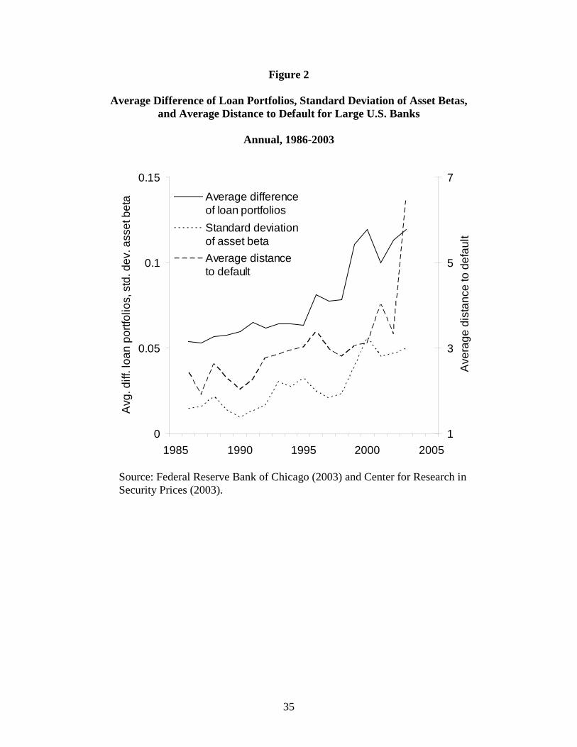
Figure 2 presents annual time-series data for 1986-2005 for the standard deviation

of the BHCs’ asset betas, the analogous cross-sectional standard deviation for BHCs’

asset volatility, and a measure of the average difference of BHCs’ loan portfolios. The

difference each year in each BHC’s loan portfolio was measured as the root mean square

of the difference between the shares of each BHC’s loan portfolio and the mean of loan

portfolio shares for each loan category across all (large) banks. (The Data Appendix,

which follows the tables below more completely defines and explains our variables and

calculations.)

For a shorter time period, Luengnaruemitchai and Wilcox (2004) compared

average capital ratios with averages and standard deviations of BHCs’ equity and asset

16

betas. They showed that lower average capital ratios are associated with (1) lower equity

betas, (2) typically less total risk taking, as measured by the average asset betas, and (3)

lower dispersion (more clustering) in risk-taking profiles across banks. By comparing

figures 1 and 2, we see that lower capital ratios are associated with more clustering, or

similarity, as measured by smaller dispersion of the asset betas. Lower capital ratios are

also associated with other measures of how much BHCs clustered.

The safety in similarity hypothesis implies that individual banks will tend to

cluster more when the banking industry generally is weaker. When the banking industry

is stronger, individual banks may maximize expected profits by adopting business

strategies and portfolios that differ more from the rest of the banking industry. When the

banking industry is weaker, individual banks have incentives, operating through reporting

discretion, to alter their risk-taking, in particular by clustering more. That is, individual

banks have incentives to converge toward the average characteristics of other banks.

“Outlier” banks then have financial motives to seek the safety of the herd, for reasons

similar to those of wildebeests, which herd together for safety on the savannah.

To more formally test whether individual banks follow the safety in similarity

hypothesis, we relate how similar a bank is to one another (here, measured by each

bank’s asset beta) to the overall strength of the banking industry (here, first measured by

the ratio of capital to assets, aggregated across the banks in our sample). In equation (2),

the first difference of the asset beta for each individual BHC i in period t ( ti,β∂ or the

difference between the current value of asset beta ( ti,β ) and its previous value ( 1, −tiβ )) is

a function of (1) the difference between the individual bank’s asset beta and the average

17

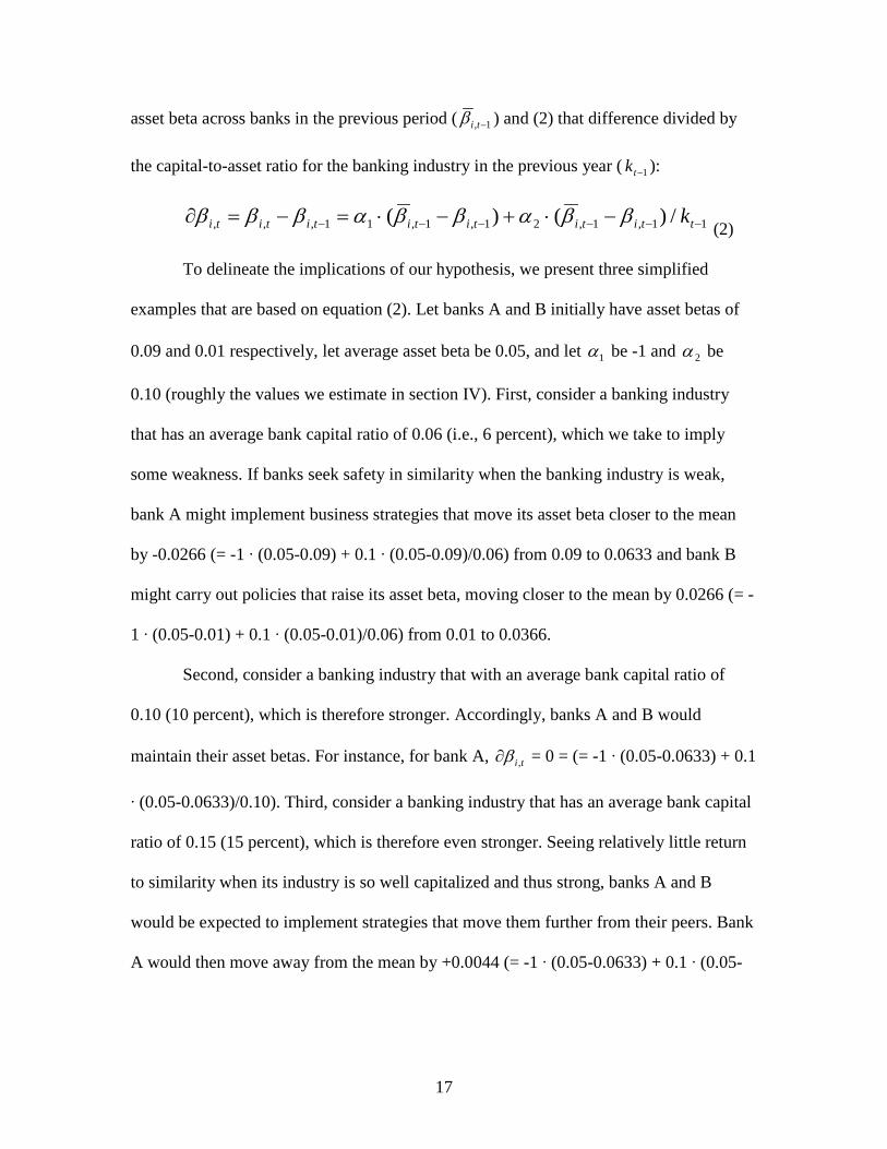
asset beta across banks in the previous period ( 1, −tiβ ) and (2) that difference divided by

the capital-to-asset ratio for the banking industry in the previous year ( 1−tk ):

11,1,21,1,11,,, /)()( −−−−−− −⋅+−⋅=−=∂ ttititititititi kββαββαβββ (2)

To delineate the implications of our hypothesis, we present three simplified

examples that are based on equation (2). Let banks A and B initially have asset betas of

0.09 and 0.01 respectively, let average asset beta be 0.05, and let 1α be -1 and 2α be

0.10 (roughly the values we estimate in section IV). First, consider a banking industry

that has an average bank capital ratio of 0.06 (i.e., 6 percent), which we take to imply

some weakness. If banks seek safety in similarity when the banking industry is weak,

bank A might implement business strategies that move its asset beta closer to the mean

by -0.0266 (= -1 ∙ (0.05-0.09) + 0.1 ∙ (0.05-0.09)/0.06) from 0.09 to 0.0633 and bank B

might carry out policies that raise its asset beta, moving closer to the mean by 0.0266 (= -

1 ∙ (0.05-0.01) + 0.1 ∙ (0.05-0.01)/0.06) from 0.01 to 0.0366.

Second, consider a banking industry that with an average bank capital ratio of

0.10 (10 percent), which is therefore stronger. Accordingly, banks A and B would

maintain their asset betas. For instance, for bank A, ti,β∂ = 0 = (= -1 ∙ (0.05-0.0633) + 0.1

∙ (0.05-0.0633)/0.10). Third, consider a banking industry that has an average bank capital

ratio of 0.15 (15 percent), which is therefore even stronger. Seeing relatively little return

to similarity when its industry is so well capitalized and thus strong, banks A and B

would be expected to implement strategies that move them further from their peers. Bank

A would then move away from the mean by +0.0044 (= -1 ∙ (0.05-0.0633) + 0.1 ∙ (0.05-

18

0.0633)/0.15) from 0.0633 to 0.0677. Bank B would also move away from the mean, but

by -0.0044 (= -1 ∙ (0.05-0.0266) + 0.1 ∙ (0.05-0.0266)/0.15) from 0.0366 to 0.0322.

We estimated equation (2) with OLS and with various panel data techniques that

included either BHC-specific dummies or year-dummies, or both. Our results were quite

robust with respect to the various estimation techniques.

Finding significantly positive coefficients for 2α implies support for the safety in

similarity hypothesis. A positive 2α implies that the weaker the banking industry (as

measured by a lower average capital ratio), the more that any individual bank changes its

strategies and portfolios in the direction of the industry averages. That is, the weaker the

industry, the more that banks clustered.

IV. Results

Tables 1 through 6 provide results that bear on the hypothesis of reporting

discretion. We present estimates based on regressions of annual charge-offs and

provisions for loan losses for the 30 largest U.S. banks for each year. We present results

for various sample periods. As noted above, we used OLS and various panel data

techniques that included either bank-specific dummies or year-dummies, or both. We

found the results to be broadly robust across those techniques, especially for the

provisions regression. We also present results for our regression specifications based on

the levels of variables and on the first-differences of each of the included variables.

In Tables 1-6, when macro controls are not included, results are presented for

regressions that included year-dummies, but do not report the coefficients and t-statistics

for the year-dummies. Data for nonaccrual loans and some other variables are not

19

available for some of the early years in the sample period. To provide estimates that do

include years before 1983 Tables 1 and 2 provide results for an abridged specification of

equation (1) that covers the entire 1978-2005 sample period. Thus, as explanatory

variables, Tables 1 and 2 include in the ‘brief’ regression each bank’s operating income,

the average capital ratio at the other 29 other banks lagged one year, and the square of

that average capital ratio. The results of an expanded regression are also included in

which each bank’s own equity capital ratio (and the square of this variable) is included as

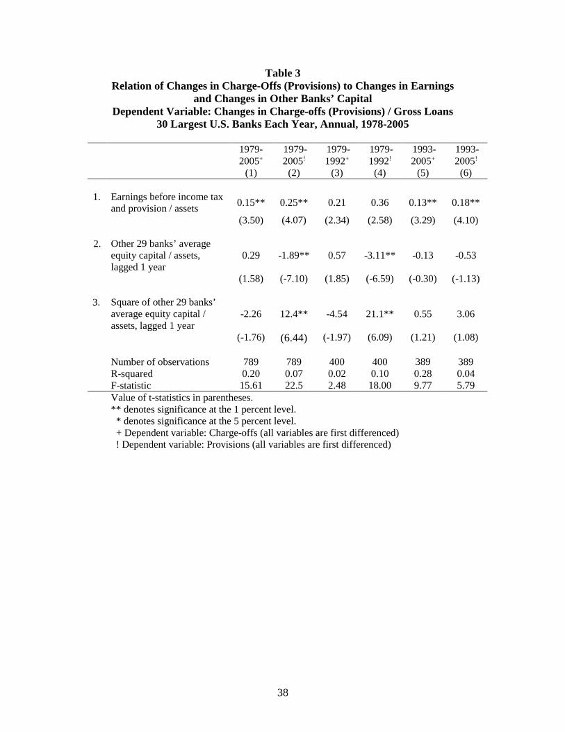
well as various macroeconomic control variables. Table 3 present the results for charge-

offs and for loan loss provisions that we obtained when we used the first-difference,

rather than the levels, specification. Table 3 contains both full (1979-2005) sample and

split (1979-1992 and 1993-2005) sample results for the first differences of charge-offs

and provisions. Tables 4 and 5 provide results for a longer specification of equation (1),

but covers only the shorter, 1985-2005 period. Table 6 contains estimated based on the

full (1979-2005) sample for the first-differenced version of the specifications for charge-

offs and for provisions.

The full-sample results in column 1 of Tables 1 and 2 generally support the

reporting discretion hypothesis. The positive and statistically very reliable (significant at

the one percent level) relation between reported charge-offs (and provisions) and

operating earnings at individual banks is consistent with lower earnings “allowing” banks

to report fewer charge-offs and provisions. On the assumption that that gross loans are

about two-thirds of bank assets, then for every extra dollar of operating income, banks

report about one-third (1/3 = 1/2 ∙ 2/3) as many charge-offs and provisions. Given that we

might expect that, absent reporting discretion, operating income might well be negatively

20

correlated with the flow of additional problem loans, the strength of this positive relation

is notable.

Moreover a positive and statistically significant coefficient (at the five percent

level) for other banks’ capital also supports the hypothesis that reporting discretion vis à

vis provisions varies inversely with the overall strength of the banking industry. On the

assumption that gross loans are about two-thirds of total bank assets, then for every extra

dollar of capital at other banks, banks reported about two-thirds (2/3=2/3*1) as much

additional provisions (and charge-offs, although this relationship is not significant in

some permutations of the model).

However, the relation between reported charge-offs (and provisions) and capital

at other banks might not be linear. Regulators, for example, might be much more

concerned about the aggregate repercussions of more charge-offs and provisions when

the banking industry is very weak. Thus, at ever lower levels of industry capital,

individual banks might respond to further declines in industry capital with ever-

increasing understatements of their own charge-offs and provisions. Conversely, at

sufficiently high levels of industry capital, individual banks might be accorded very little

reporting discretion. Thus, to investigate this possibility, we add the square of capital at

other banks in the full sample regressions. As another way to investigate the possibility of

nonlinearities, in columns 3 through 6, we present the results of regressions performed

over sub-samples that differed in their average macroeconomic and banking industry

strength.

The results for the quadratic specification are even stronger than those for the

linear specification: The coefficients for the square of other banks’ capital are significant

21

at the one percent level. The magnitudes of the coefficients for the linear and quadratic

terms imply (1) that banks respond by reporting fewer charge-offs and provisions when

other banks have less capital for capital ratios between 0 and 9 percent and (2) that the

amounts of reporting discretion, while rising very sharply as capital ratios approach zero,

dwindle to zero when the banking-industry-wide capital ratio is about 9 percent.

We also estimated the specification for four sub-periods (1978-1984, 1985-1991,

1992-1998, and 1999-2005). These sub-periods differ in their average strength of the U.S.

banking system. One notable difference is shown in Figure 1: The average bank capital

ratio was much lower before the mid-1980s and much higher after the mid-1990s. In

addition, the 1978-1984 sub-period includes high inflation, high unemployment, a

double-dip recession, but relatively few bank loan charge-offs. The 1985-1991 sub-period

also includes a recession, but is distinguished by its severe banking crisis and historically

high charge-offs. The 1992-1998 sub-period includes a long and vigorous economic

expansion, low inflation, and low charge-offs. The 1999-2005 sub-period covers the most

recent economic experience, including booms and/or busts in various asset markets, fairly

low inflation, the end of an economic expansion, a mild recession, the beginning of the

current expansion, and relatively low charge offs.

Columns 3 through 6 of Tables 1 and 2 show that the responses of reported

charge-offs and provisions to individual-bank’s operating earnings and other banks’

capital vary across sub-periods. This is what the quadratic form led us to expect. The

coefficients for operating income are roughly similar across sub-periods and are

significant at the one percent level almost always (and always at the ten percent level). In

contrast, the coefficients on other banks’ capital are much larger and more statistically

22

significant for the 1985-1991 period, which had both low aggregate capital and high

charge-offs. The coefficients for other banks’ capital are statistically weakest for the

periods with the lowest charge-offs (1978-1983) or when the memory of extremely high

charge-offs has dissipated (1999-2005). The first-difference results shown in Table 3

generally follow a similar pattern to those in Tables 1 and 2. Charge-offs and provisions

both tend to rise with banks’ reported (pre-provision) profits. Particularly for provisions,

the results in Table 3 suggested that banks tended to provision less (having factored in the

effects of other banks’ capital working through the level and squared terms, again

particularly during the pre-FDICIA period, when the banking industry was weaker.

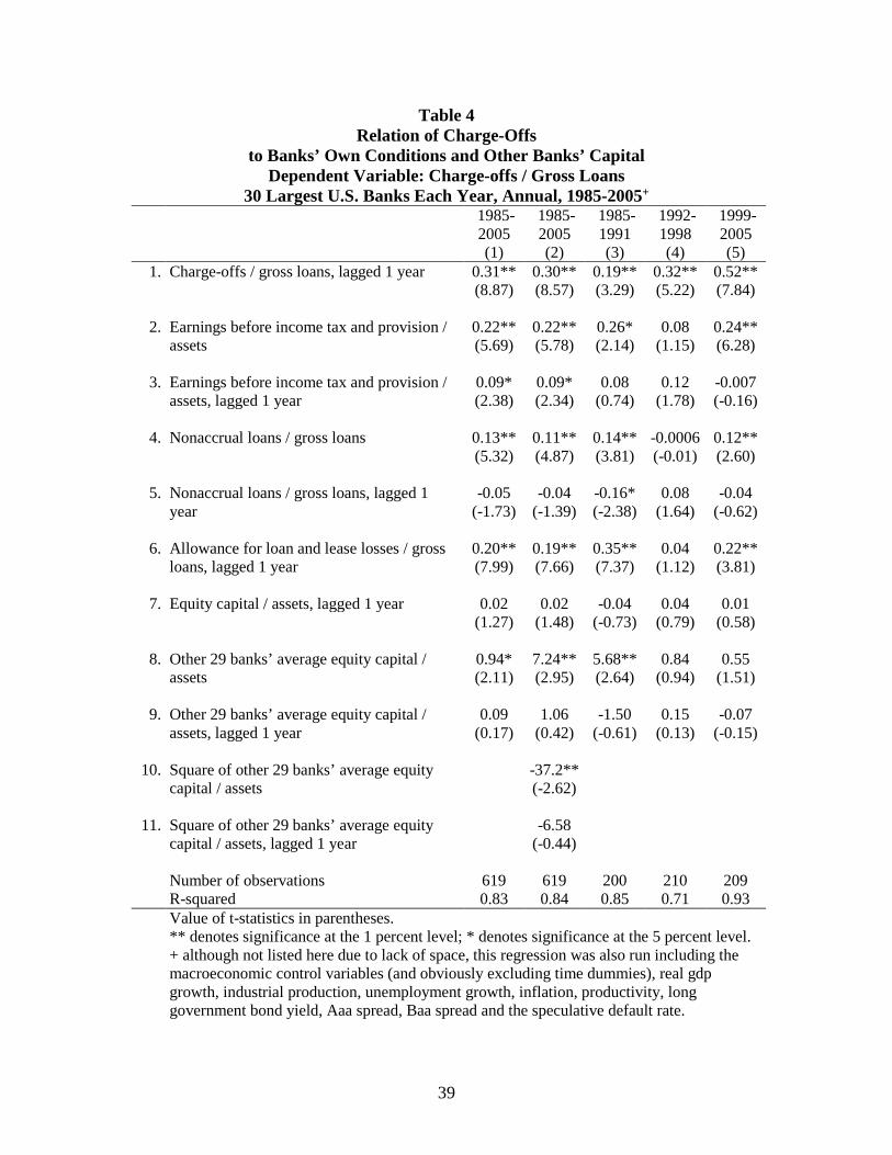
Tables 4 and 5 provide additional support for the earlier finding that, all else

equal, individual banks tend to and provision (and to a lesser degree charge-off) less

when the banking industry is weaker. Tables 4 and 5 provide the results of the full model

presented in equation (1). Thus, the same dependent variables are regressed on more

control variables for the 1985-2005 period, with macro variables excluded (column 1)

and included (Column 2). The full linear specification was also estimated over three sub-

periods (1985-1991, 1992-1998, and 1999-2005).

Our confidence in the estimated effects of capital is bolstered by the general

pattern of other coefficients. For example, in general, charge-offs and provisions are

systematically higher, all else equal, when banks’ operating incomes are higher, when

nonaccrual loans were higher, and when banks’ own loan loss allowances were higher.

The estimated coefficients on operating earnings are positive and significant for the full

sample (1985-2005) and for two of three sub-periods (1985-1991 and 1999-2005). The

estimated coefficients on loan loss allowances (lagged one-year) in the charge-off

23

equations are consistently positive and significant (except in the 1992-1998 sub-period),

indicating that larger stocks of loss reserves imply that banks later will take larger charge-

offs. In contrast, the coefficients on loan loss allowances in the provisions equations and

on lagged own-capital are largely insignificant.

We found no consistent relation between banks’ own capital and their charge-offs

and provisions. Having controlled for the own capital effect, which received only

moderate statistical endorsement, we are more confident in our estimates of the effects of

other banks’ capital.

The estimated coefficients on other banks’ capital are positive and significant (at

the five percent level) in the linear specification (columns 1 of Tables 4 and 5) and (at the

one percent level) in the quadratic equation (columns 2 of Tables 4 and 5). The

magnitudes of the capital coefficients in the quadratic specifications imply, as did Tables

1 and 2, the amounts by which banks under-report charge-offs and provisions rise sharply

as other banks’ capital ratios fall to very low levels, and that the amounts of under-

reporting dwindles to near zero at aggregate capital ratios between 9 and 10 percent. The

sub-period estimates show that the coefficients for other banks’ capital are larger and

statistically more significant for the 1985-1991 period than for the two subsequent sub-

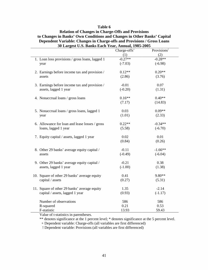
periods (1992-1998 and 1999-2005). Table 6 presents the results of estimating full-

sample, first-differenced versions of the specifications in Tables 4 and 5. Relative to the

levels specification, the first-differenced specification provided little signal that charge-

offs responded to industrywide banking strength. By contrast, column 2 shows that, even

in the first-differenced specification, the combination of the estimated coefficients on

other banks’ capital ratios in levels and squares clearly indicated that loss provisions at

24

individual banks tended to decline as the banking industry weakened. Thus, overall,

Tables 1-6 provide considerable support for the hypothesis that banks systematically

reported fewer charge-offs and provisions when the banking industry was weaker.

Tables 7-9 provide results that support the safety in similarity, or clustering,

hypothesis. Table 7 presents results based on OLS time-series regressions that use data

for annual, aggregate conditions for the top 30 BHCs for 1987-2003. As dependent

variables, we used four different measures of the extent to which banks were similar, or

clustered, in their risk-taking. Three measures are based on stock market data: the (cross-

sectional) standard deviation of equity betas, the standard deviation of asset betas, and the

standard deviation of a measure of the volatility of the market value of banks’ assets. A

fourth measure of the similarity of risk-taking at BHCs, the average difference of loan

portfolios, is based on the shares of assets allocated to various categories of loans. As

each of these dispersion measures increases, the similarity, or clustering, of BHCs

declines.

As independent variables in the regressions shown in Table 7, we use again use

measures of the strength of the banking industry. In addition to estimating the effects of

the industry-average capital-to-asset ratio (lagged one year), we alternatively use a

measure of the average distance to default (lagged one year) as a measure of strength.

We seek to determine whether BHCs (hereafter banks) are more similar when the

banking industry is weaker. In response to weakness, banks might not only cluster more,

but might also change (either up or down) the average amounts of risk that they take. To

examine whether it is empirically relevant to control for the extent to which average risk

taking changed as the banking industry weakened, we performed regressions both with

25

and without average asset beta as a variable. We report the estimated coefficients for the

average of banks’ asset betas, but note that omitting them did not much affect the size or

significance of the coefficients that measure the strength of the banking industry.

The results in Table 7 quite consistently support the safety in similarity, or

clustering, hypothesis. Regardless of whether we use the average capital ratio or the

approximation to distance to default, and regardless of which of four candidates we use to

serve as a proxy for the degree of dispersion of banks around the banking industry mean,

the coefficients on the measure of banking industry strength had consistently positive and

significant (almost always at the one percent level) estimated coefficients.

The results in Table 7 can be viewed as a first step toward documenting the casual

conclusion suggested by Figures 1 and 2 that the weaker that the U.S. banking industry

was, the greater was the clustering of individual banks’ betas. We take the lower standard

deviations of asset betas across banks to imply that banks are more clustered. The lower

are capital ratios, the lower too are the standard deviations of asset betas. Thus, the

largest U.S. banks tended to cluster more when their industry was weaker.

In Table 8, we used only data for non-BHC financial corporations, rather than

BHCs. In the absence of a regulatory reporting incentive that we argue applies to banking

firms, we would expect to find much less evidence of clustering. Table 8 uses the same

sample period and the measures of dispersion, capital, and betas that are conceptually the

same as those that we used for banks in Table 7. In short, we found very little indication

that non-BHC financial corporations tended to cluster more as their sector weakened. The

t-statistics on lagged capital ratios and on our distance-to-default measures barely reach

one. Thus, while the estimates suggest that BHCs did cluster as banking weakened, we

26

see very little indication in Table 8 that non-BHC financial corporations exhibited

similarly clustering.

The results presented in Table 9 take yet another step. The regressions in Table 9

use annual data for each of the individual BHCs to estimate the model in equation (2).

The dependent variable for the regressions in Table 9 is the year-on-year first-difference

in the asset beta for each of the top 30 BHCs for each year from 1987-2003. The key

independent variable in these regressions is the deviation of each individual BHC’s asset

beta from each year’s average asset beta, divided by each year’s average of the capital-to-

total asset ratio (lagged one year).

We used OLS and various panel data techniques, including either BHC-specific

dummies or year-dummies, or both. The results for our focus variable were fairly robust

across those specifications. In columns 1 and 2 of Table 9, we present full results for OLS

regressions. In columns 3 and 4 of Table 9, we present results for regressions that

included both BHC-specific-dummies and year-dummies. We do not report the

coefficients and t-statistics for the BHC-specific-dummies and the year-dummies.

The positive and significant coefficients in row 3 imply that individual BHCs

whose asset betas differed from the average asset beta for that year responded to lower

levels of banking industry capital by moving their strategies and portfolios closer to the

industry averages. Banks that had asset betas below the average moved them up and they

moved them up more, the lower was the aggregate capital ratio. Thus, when the banking

industry weakened, individual banks tended to cluster more.

The magnitudes of the coefficients in row 3 for columns 1 and 3 imply that the

impetus to cluster dwindles to zero by the time the aggregate capital ratio is in the range

27

of 9-11 percent. The further that capital falls, however, the more that individual banks

tend to cluster.

As an additional control, we added to the specifications used for columns 1 and 3

a variable that divided the deviation of the individual from the average asset beta by each

individual bank’s capital ratio. We present the results in columns 2 and 4 of Table 9.

While the estimated effects of this additional variable seemed quite sensitive to the

presence of dummy variables, the effects of banking industry capital on the asset betas of

individual banks was not sensitive: The effects of banking industry capital remained

sizable and significant, regardless of whether the own capital variable was included.

V. Summary and implications

In this paper we provide evidence that the largest U.S. banks have tended to report

both lower charge-offs and provisions for loan losses, after controlling for their other

determinants, when other banks were weaker. We then argued that this reporting

discretion provides banks with incentives to cluster more when the banking industry is

weaker. We then show that banks tended to be more clustered, or similar, when the

banking industry is weaker. In addition, we showed that individual banks detectably

changed their risk-taking to become more like that of other banks during periods when

the banking industry is weaker. We also showed that the weaker the banking industry is,

the more that individual banks changed their business strategies and portfolios, as

measured by their asset betas. The results based on non-BHC financial corporations

further support our perspective. Our results based on non-BHC corporations gave little or

28

no indication that they tended to cluster more as their part of the financial sector

weakened.

While the results for non-BHC corporations suggest that the banking industry is

unique in that risk dispersion decreases as the industry weakens, the results do not

exclude other interpretations (beyond banks actively seeking similarity) for this

relationship. It is plausible that the riskiness of banks and a tendency to move together

might be related due to circumstances beyond the banks’ control. For instance, one

stylized fact is that measured asset price correlations increase in times of high volatility.

However if this were the underlying cause for the relationship observed, then we might

expect that the relationship would also hold true for non-financials as well (which we do

not find). However, there maybe other reasons the relationship is specific to the banking

industry. For instance, banks may be supported by the government (or the market may

view this as being true even if it is not) when bank capital has been sufficiently depleted

by a series of negative shocks. In this case the safety net of the government may respond

to common shocks more than to individual risk factors. Thus the appearance would be

that banks cluster more in times of distress than when the industry was healthy. While

our results are consistent with one theory of bank herding behavior, we acknowledge that

other theories may be plausible given the results.

Banks typically come under capital pressure, for instance, either because large

loan losses reduce their capital or because changes in rules and regulations raise the

amounts of capital that they are required to hold. In turn, capital pressures can lead to

reductions in banks’ supply of loans. Regulatory requirements may also require capital to

rise promptly as expected loan losses rise, for example during recessions. In that case,

29

bank lending might become more procyclical than when required capital responds less to

current conditions. To reduce the procyclicality of regulatory capital requirements, some

argue for including “escape clauses.” Such clauses might, for example, require bank

capital to rise during expansions, but perhaps allow it to fall during downturns.

Likewise, discretion in banks’ reporting of charge-offs and provisions may reduce

the procyclicality of an otherwise fixed set of banking regulations. Banks may be

permitted to exercise more discretion in their reporting of charge-offs and provisions

when the banking system is weaker than when problems are more isolated. Such

discretion has the desired effect of at least temporarily preserving financial stability. As

we show, it may also encourage banks to cluster to gain “safety in similarity.” Whether

more clustering adds to financial stability is an open question.

The Prompt Corrective Action (PCA) clauses of FDICIA seek to minimize future

banking crises and deposit insurer losses. PCA generally requires that restrictions on

banks become increasingly severe as their capital ratios fall below various trigger ratios.

In part, PCA is designed to reduce both the need and opportunities for regulatory

forbearance. However, PCA and similarly triggered policies might be undermined by

reporting discretion that allows banks to report sufficiently high capital to avoid PCA’s

being triggered. The hypothesis of reporting discretion posits that underreporting of

problem loans is most likely to occur exactly at the times when banks are most likely to

otherwise trigger PCA’s restrictions. In that sense, reporting discretion has the potential

to replace “first generation” forbearance with a second generation of forbearance that

might be more difficult those who are neither bankers nor bank regulators to detect.

30

Reporting discretion could have other consequences as well. Some bank

regulators might be skeptical of being asked to manage or even being perceived as

managing, macroeconomic outcomes. Allowing banks discretion in their reporting might

(1) later reduce the discipline of banks’ credit monitoring, (2) lead ultimately to larger

average amounts of problem loans, and (3) ultimately divert credit from its most efficient

uses. As a consequence, discretion in banks’ reporting of charge-offs and loan loss

provisions might exacerbate (unexpected and expected) losses to banks and their deposit

insurers. In addition, monetary authorities may recognize that bank supervisors might

respond to contractionary monetary policy by allowing banks to exercise more discretion,

for example by permitting banks to “evergreen” or avoid charging-off loans. Inconsistent

application of such discretion by bank regulators might also confound appropriate

application of countercyclical monetary policy. To the extent that the amounts and effects

of such reporting discretion are hard to quantify and predict, monetary policy would be

that much harder to conduct.

Although we found less evidence of reporting discretion in more recent sub-

periods, reporting discretion might well emerge during future banking crises.9 In the 15

years since FDICIA was enacted, banking has been very profitable and capital ratios have

risen to their highest levels in more than a generation. Under such conditions, there is

little demand by individual banks or supply by regulators of reporting discretion. Under

such conditions, the incentives to cluster to gain “safety in similarity” would be minor.

However, should conditions change in the future, the responses of banks and their

regulators could change as well.

31

Because of the macroeconomic repercussions of banking difficulties, it may be

socially optimal that reporting discretion of the sort discussed here does emerge. If so, it

may also be preferable that it be practiced consciously and consistently so that the

policies of both private-sector banks and public-sector policymakers can better coordinate

their general policies and specific responses. Acknowledging and measuring the

magnitudes of reporting discretion that occurred in the past is a first step toward more

coherent policies in both the private and public sector.

32

References

Acharya, V.V., Yorulmazer T., 2004. Too Many to Fail – An Analysis of Time-inconsistency in Bank Closure Regulation. Unpublished Manuscript, London Business School.

Ahmed, A.S., Takeda, C., Thomas, S., 1999. Bank Loan Loss Provisions: Reexamination

of Capital Management, Earnings Management and Signaling Effects. Journal of Accounting and Economics 28, 1-25.

Allen, L., Saunders, A., 2004. Incorporating Systemic Influences into Risk

Measurements: A Survey of the Literature. Journal of Financial Services Research 26: 2, 61-192.

Basu, S., 1997. The Conservatism Principle and the Asymmetric Timeliness of Earnings.

Journal of Accounting and Economics 24, 3-37. Berger, A., Kyle, M. and J Scalise, 2000, Did U.S. Bank Supervisors Get Tougher During

the Credit Crunch? Did They Get Easier During the Banking Boom? Did it Matter to Bank Lending? In Frederic Mishkin, Ed. Prudential Supervision: What Works and What Doesn’t: University of Chicago Press.

Bernanke, B., Lown C.S., 1991. The Credit Crunch. Brookings Papers on Economic

Activity, 205-239. Bliss, R., Kaufman, G., Smith J., 2002. Explaining Bank Credit Crunches and

Procyclicality. The Federal Reserve Bank of Chicago. Chicago Fed. Letter 179. Flannery, M.J., Rangan K.P., 2003. What Caused the Bank Capital Build-Up of the

1990s? Working Paper. Department of Finance, Insurance and Real Estate Graduate School of Business, University of Florida. Green, E., Lopez, J., Wang, Z., 2001. “The Federal Reserve Banks’ Imputed Cost of

Equity Capital,” Working Paper, Federal Reserve Bank of San Francisco, San Francisco, CA.

Hanc, G., 1998. The Banking Crises of the 1980s and Early 1990s: Summary and

Implications. FDIC Banking Review, 11: 1. Hasan, Iftekhar and Larry Wall, 2003, Determinants of the Loan Loss Allowance: Some

Cross-Country Comparisons, Bank of Finland Discussion Papers. Hovakimian, A., Kane E.J., 2000. Effectiveness of Capital Regulation at U.S.

Commercial Banks, 1985 to 1994. The Journal of Finance, LV: 1.

33

Ioannidou, V.P., 2004. Does Monetary Policy Affect the Central Bank’s Role in Bank Supervision? Journal of Financial Intermediation, 14: 1, 58-85.

Kane, E. J., 1987. Dangers of Capital Forbearance: the Case of the FSLIC and Zombie

S&Ls. Contemporary Policy Issues 5, 77-83. Kane, E. J., 1989. The S&L Insurance Mess: How Did it Happen? Urban Institute Press,

Washington, D.C. Laeven, L., Majnoni G., 2003. Loan Loss Provisioning and Economic Slowdowns: Too

Much, Too Late? Journal of Financial Intermediation 12, 178-197. Luengnaruemitchai, P. Wilcox, J., 2004. Pro-cyclicality, Banks’ Reporting Discretion,

and “Safety in Similarity” in The New Basel Accord, edited by Benton E. Gup, South-Western Publishing, 151-175.

Merton, R., 1974, “On the Pricing of Corporate Debt: The Risk Structure of Interest

Rates,” Journal of Finance 29, 449-470. Pennacchi, G., 2005a. Deposit Insurance, Bank Regulation, and Financial System Risk.

Carnegie-Rochester Series Conference (Spring). Pennacchi, G., 2005b. Risk-based Capital Standards, Deposit Insurance, and

Procyclicality. Journal of Financial Intermediation 14, 432-465. Van der Heuvel, S. J., 2002. Does Bank Capital Matter for Monetary Policy? Federal

Reserve Bank of New York, Economic Policy Review (May), 259-265.

34

Figure 1

Charge-offs, Provisions, and Average Equity Capital Ratio for Large U.S. Banks

Annual, 1976-2005

Source: Federal Reserve Bank of Chicago (2005).

0

1

2

3

4

1975 1980 1985 1990 1995 2000 2005

Pro

visi

ons

and

char

ge o

ffs p

er g

ross

loan

s (%

)

2

4

6

8

10

Equ

ity p

er to

tal a

sset

s (%

)

ProvisionsCharge-offsEquity

35

Figure 2

Average Difference of Loan Portfolios, Standard Deviation of Asset Betas, and Average Distance to Default for Large U.S. Banks

Annual, 1986-2003

Source: Federal Reserve Bank of Chicago (2003) and Center for Research in Security Prices (2003).

0

0.05

0.1

0.15

1985 1990 1995 2000 2005

Avg

. diff

. loa

n po

rtfol

ios,

std

. dev

. ass

et b

eta

1

3

5

7

Ave

rage

dis

tanc

e to

def

ault

Average differenceof loan portfolios Standard deviationof asset betaAverage distanceto default

36

Table 1 Relation of Charge-Offs to Earnings and Other Banks’ Capital

Dependent Variable: Charge-offs / Gross Loans 30 Largest U.S. Banks Each Year, Annual, 1978-2005

1978-2005

1978-2005

1978-1984

1985-1991

1992-1998

1999-2005

(2) (2) (3) (4) (5) (6) 1. Constant -0.42** -0.01 -0.09 -0.37** -0.06 -0.05

(-5.08) (-0.35) (-1.17) (-3.96) (-1.01) (-1.03)

2. Earnings before income tax and provision / assets

0.44** 0.38** 0.37 0.28** 0.24** 0.52**

(18.0) (14.18) (1.96) (4.07) (3.67) (19.6)

3. Other 29 banks’ average

equity capital / assets, lagged 1 year

9.83** 0.35 2.08 7.33** 0.75 0.44

(4.78) (0.95) (1.23) (4.10) (1.03) (0.92)

4. Square of other 29 banks’

average equity capital / assets, lagged 1 year

-56.6** -5.47*

(-4.35) (-1.88)

5. Own equity capital/assets, lagged 1 year -0.45**

(-7.59)

6.

Square of own equity capital/assets lagged 1 year

2.23**

(7.15) 7. Real GDP Growth 0.00 (0.45) 8. Inflation -0.00 (-0.36) 9. Productivity -0.00 (-1.78) 10. Speculative Default Rate 0.00** (7.37) - Other macro effects+ Number of observations 829 829 210 200 210 209 R-squared 0.20 0.40 0.16 0.30 0.28 0.69 F-statistic 22.0 28.2 4.68 9.99 9.77 56.1 Value of t-statistics in parentheses.

** denotes significance at the 1 percent level. * denotes significance at the 5 percent level. + other variables tested includes industrial production, unemployment, long government bond yield, Aaa spread, and Baa spread.

37

Table 2 Relation of Loan Loss Provisions to Earnings and Other Banks’ Capital

Dependent Variable: Loan Loss Provisions / Gross Loans 30 Largest U.S. Banks Each Year, Annual, 1978-2005

1978-2005

1978-2005

1978-1984

1985-1991

1992-1998

1999-2005

(2) (2) (3) (4) (5) (6) 1. Constant -0.34** -0.05** -0.12 -0.19 -0.09 -0.06

(-3.47) (-2.58) (-1.35) (-1.62) (-1.88) (-1.26)

2. Earnings before income tax and provision / assets

0.49** 0.45** 0.88** 0.23** 0.31** 0.57**

(17.1) (13.32) (3.91) (2.63) (4.97) (19.8)

3. Other 29 banks’ average

equity capital / assets, lagged 1 year

7.49** 1.39** 2.75 3.95 1.32 0.60

(3.13) (2.96) (1.35) (1.74) (1.87) (1.13)

4. Square of other 29 banks’

average equity capital / assets, lagged 1 year

-42.0** -12.6**

(-2.77) (-3.41)

5. Own equity capital/assets, lagged 1 year -0.33**

(-4.65)

6.

Square of own equity capital/assets lagged 1 year

1.72**

(4.31) 7. Real GDP Growth 0.00** (5.12) 8. Inflation 0.00** (2.44) 9. Productivity -0.00** (-3.21) 10. Speculative Default Rate 0.00** (7.50) - Other macro effects+ Number of observations 829 829 210 200 210 209 R-squared 0.25 0.35 0.18 0.35 0.30 0.69 F-statistic 25.1 29.1 5.60 12.8 10.61 56.0 Value of t-statistics in parentheses.

** denotes significance at the 1 percent level. *denotes significance at the 5 percent level. + other variables tested includes industrial production, unemployment, long government bond yield, Aaa spread, and Baa spread.

38

Table 3 Relation of Changes in Charge-Offs (Provisions) to Changes in Earnings

and Changes in Other Banks’ Capital Dependent Variable: Changes in Charge-offs (Provisions) / Gross Loans

30 Largest U.S. Banks Each Year, Annual, 1978-2005

1979-2005+

1979-2005!

1979-1992+

1979-1992!

1993-2005+

1993-2005!

(1) (2) (3) (4) (5) (6)

1. Earnings before income tax and provision / assets 0.15** 0.25** 0.21 0.36 0.13** 0.18**

(3.50) (4.07) (2.34) (2.58) (3.29) (4.10)

Other 29 banks’ average equity capital / assets, lagged 1 year

2.

0.29 -1.89** 0.57 -3.11** -0.13 -0.53

(1.58) (-7.10) (1.85) (-6.59) (-0.30) (-1.13)

Square of other 29 banks’ average equity capital / assets, lagged 1 year

3.

-2.26 12.4** -4.54 21.1** 0.55 3.06

(-1.76) (6.44) (-1.97) (6.09) (1.21) (1.08)

Number of observations

789 789 400 400 389 389 R-squared 0.20 0.07 0.02 0.10 0.28 0.04 F-statistic 15.61 22.5 2.48 18.00 9.77 5.79 Value of t-statistics in parentheses.

** denotes significance at the 1 percent level. * denotes significance at the 5 percent level. + Dependent variable: Charge-offs (all variables are first differenced) ! Dependent variable: Provisions (all variables are first differenced)

39

Table 4 Relation of Charge-Offs

to Banks’ Own Conditions and Other Banks’ Capital Dependent Variable: Charge-offs / Gross Loans

30 Largest U.S. Banks Each Year, Annual, 1985-2005+

1985-2005

1985-2005

1985-1991

1992-1998

1999-2005

(1) (2) (3) (4) (5) 1. Charge-offs / gross loans, lagged 1 year 0.31** 0.30** 0.19** 0.32** 0.52**

(8.87) (8.57) (3.29) (5.22) (7.84)

2. Earnings before income tax and provision / assets

0.22** 0.22** 0.26* 0.08 0.24** (5.69) (5.78) (2.14) (1.15) (6.28)

3. Earnings before income tax and provision / assets, lagged 1 year

0.09* 0.09* 0.08 0.12 -0.007 (2.38) (2.34) (0.74) (1.78) (-0.16)

4. Nonaccrual loans / gross loans 0.13** 0.11** 0.14** -0.0006 0.12** (5.32) (4.87) (3.81) (-0.01) (2.60)

5. Nonaccrual loans / gross loans, lagged 1 year

-0.05 -0.04 -0.16* 0.08 -0.04 (-1.73) (-1.39) (-2.38) (1.64) (-0.62)

6. Allowance for loan and lease losses / gross loans, lagged 1 year

0.20** 0.19** 0.35** 0.04 0.22** (7.99) (7.66) (7.37) (1.12) (3.81)

7. Equity capital / assets, lagged 1 year 0.02 0.02 -0.04 0.04 0.01 (1.27) (1.48) (-0.73) (0.79) (0.58)

8. Other 29 banks’ average equity capital / assets

0.94* 7.24** 5.68** 0.84 0.55 (2.11) (2.95) (2.64) (0.94) (1.51)

9. Other 29 banks’ average equity capital / assets, lagged 1 year

0.09 1.06 -1.50 0.15 -0.07 (0.17) (0.42) (-0.61) (0.13) (-0.15)

10. Square of other 29 banks’ average equity capital / assets

-37.2** (-2.62)

11. Square of other 29 banks’ average equity capital / assets, lagged 1 year

-6.58 (-0.44) Number of observations 619 619 200 210 209 R-squared 0.83 0.84 0.85 0.71 0.93 Value of t-statistics in parentheses. ** denotes significance at the 1 percent level; * denotes significance at the 5 percent level.

+ although not listed here due to lack of space, this regression was also run including the macroeconomic control variables (and obviously excluding time dummies), real gdp growth, industrial production, unemployment growth, inflation, productivity, long government bond yield, Aaa spread, Baa spread and the speculative default rate.

40

Table 5 Relation of Loan Loss Provisions

to Banks’ Own Conditions and Other Banks’ Capital Dependent Variable: Loan Loss Provisions / Gross Loans

30 Largest U.S. Banks Each Year, Annual, 1985-2005+

1985-2005

1985-2005

1985-1991

1992-1998

1999-2005

(1) (2) (3) (4) (5) 1. Loan loss provisions / gross loans, lagged 1

year 0.33** 0.32** 0.15 0.36** 0.63**

(8.16) (7.82) (1.73) (6.15) (9.53)

2. Earnings before income tax and provision / assets

0.27** 0.29** 0.39* 0.13 0.28** (5.60) (6.03) (2.37) (1.84) (5.78)

3. Earnings before income tax and provision / assets, lagged 1 year

0.12* 0.11* -0.01 0.06 -0.01 (2.40) (2.21) (-0.08) (0.89) (-0.24)

4. Nonaccrual loans / gross loans 0.31** 0.29** 0.37** 0.06 0.35** (10.5) (9.83) (7.34) (1.15) (5.82)

5. Nonaccrual loans / gross loans, lagged 1 year

-0.19** -0.17** -0.26** 0.04 -0.34** (-4.91) (-4.35) (-2.78) (0.77) (-3.72)

6. Allowance for loan and lease losses / gross loans, lagged 1 year

-0.02 -0.02 0.03 -0.08* 0.04 (-0.48) (-0.78) (0.48) (-2.26) (0.65)

7. Equity capital / assets, lagged 1 year 0.02 0.02 0.07 0.04 -0.01 (1.04) (1.09) (0.77) (0.87) (-0.44)

8. Other 29 banks’ average equity capital / assets

1.40* 15.6** 13.0** 1.24 0.26 (2.51) (5.13) (4.47) (1.35) (0.56)

9. Other 29 banks’ average equity capital / assets, lagged 1 year

0.03 -4.59 -5.01 0.51 0.38 (0.04) (-1.47) (-1.52) (1.44) (0.65)

10. Square of other 29 banks’ average equity capital / assets

-83.5** (-4.75)

11. Square of other 29 banks’ average equity capital / assets, lagged 1 year

-27.0 (1.44) Number of observations 619 619 200 210 209 R-squared 0.80 0.81 0.83 0.64 0.91 Value of t-statistics in parentheses. ** denotes significance at the 1 percent level; * denotes significance at the 5 percent level.

+ although not listed here due to lack of space, this regression was also run including the macroeconomic control variables (and obviously excluding time dummies) real gdp growth, industrial production, unemployment growth, inflation, productivity, long government bond yield, Aaa spread, Baa spread and the speculative default rate.

41

Table 6 Relation of Changes in Charge-Offs and Provisions

to Changes in Banks’ Own Conditions and Changes in Other Banks’ Capital Dependent Variable: Changes in Charge-offs and Provisions / Gross Loans

30 Largest U.S. Banks Each Year, Annual, 1985-2005 Charge-offs+ Provisions!

(1) (2) 1. Loan loss provisions / gross loans, lagged 1

year -0.27** -0.28**

(-7.03) (-6.98)

2. Earnings before income tax and provision / assets

0.12** 0.20** (2.86) (3.76)

3. Earnings before income tax and provision / assets, lagged 1 year

-0.01 0.07 (-0.20) (1.31)

4. Nonaccrual loans / gross loans 0.16** 0.40** (7.17) (14.83)

5. Nonaccrual loans / gross loans, lagged 1 year

0.03 0.09** (1.01) (2.33)

6. Allowance for loan and lease losses / gross loans, lagged 1 year

0.22** -0.34** (5.58) (-6.70)

7. Equity capital / assets, lagged 1 year 0.02 0.01 (0.84) (0.26)

8. Other 29 banks’ average equity capital / assets

-0.11 -1.66** (-0.49) (-6.04)

9. Other 29 banks’ average equity capital / assets, lagged 1 year

-0.21 0.38 (-1.00) (1.38)

10. Square of other 29 banks’ average equity capital / assets

0.41 9.80** (0.27) (5.31)

11. Square of other 29 banks’ average equity capital / assets, lagged 1 year

1.35 -2.14 (0.93) (-1.17) Number of observations 586 586 R-squared 0.21 0.53 F-statistic 13.93 59.43 Value of t-statistics in parentheses. ** denotes significance at the 1 percent level; * denotes significance at the 5 percent level.

+ Dependent variable: Charge-offs (all variables are first differenced) ! Dependent variable: Provisions (all variables are first differenced)

42

Table 7 Relation of the Clustering of BHCs to Average BHC Strength

Dependent Variables: Average Measures of BHC Dispersion (or Clustering), Annual, 1987-2003

Standard deviation of equity beta

Standard deviation of asset beta

Standard deviation of

asset volatility

Average difference of

loan portfolios (1) (2) (3) (4) (5) (6) (7) (8)

1. Constant -0.09 0.10 -0.03 0.004 -0.03 0.01 -0.01 0.05* (-1.05) (1.54) (-2.07) (0.31) (-1.36) (0.34) (-0.40) (2.81)

2. Average capital to asset ratio, lagged 1 year

5.95** 0.95** 1.14** 1.81** (4.55) (4.52) (3.24) (6.05)

3. Average distance to default, lagged 1 year

0.46** 0.07** 0.09* 0.12** (4.11) (3.28) (2.84) (3.71)

4. Average asset beta -0.59 0.48 -0.12 0.06 -0.31 -0.10 -0.49* -0.14 (-0.76) (0.65) (-0.99) (0.44) (-1.48) (-0.50) (-2.75) (-0.63) Number of observations 17 17 17 17 17 17 17 17 R-squared 0.62 0.58 0.61 0.46 0.43 0.37 0.72 0.50 F-statistic 11.6 9.53 11.1 5.98 5.25 4.04 18.3 6.88 Value of t-statistics in parentheses. ** denotes significance at the 1 percent level; * denotes significance at the 5 percent level. The coefficients for row 3 were multiplied by one million.

43

Table 8 Relation of the Clustering of non-BHC Financials to Their Average Strength

Dependent Variables: Average Measures of non-BHC Financials Dispersion (or Clustering), Annual, 1987-2003

Standard deviation of equity beta

Standard deviation of asset beta

Standard deviation of

asset volatility (1) (2) (3) (4) (5) (6)

1. Constant 0.64 0.71 0.21 0.21 0.09 0.27 (6.78) (6.87) (4.47) (3.97) (1.46) (3.70)

2. Average capital to asset ratio, lagged 1 year

0.06 0.17 0.52* (0.19) (1.04) (2.53)

3. Average distance to default, lagged 1 year

-0.00 0.00 -0.00 (-0.45) (1.01) (-0.57)

4. Average asset beta -0.16 -0.29 0.21 0.37 -0.27 -0.27 (-1.00) (-1.01) (2.62) (2.53) (-2.55) (-1.32) Number of observations 17 17 17 17 17 17 R-squared 0.32 0.05 0.26 0.25 0.26 0.08 F-statistic 0.52 0.72 5.55 4.87 5.04 1.21 Value of t-statistics in parentheses. ** denotes significance at the 1 percent level; * denotes significance at the

5 percent level. The coefficients for row 3 were multiplied by one million.

44

Table 9 Relation of Changes in Individual BHC Risk-Profiles to Average BHC Strength

Dependent Variable: First Differences of Asset Beta 30 Largest U.S. BHCs Each Year, Annual, 1987-2003

No dummy variables

BHC and year dummy variables

(1) (2) (3) (4) 1. Constant 0.00009 0.0003 0.02 0.03

(0.97) (0.35) (0.84) (1.12)

2. Deviation of own asset beta -1.08** -0.95** -0.81 -0.74 (-6.17) (-5.27) (-1.54) (-1.43)

3. Deviation of own asset beta divided by industry-average capital to total asset ratio

0.10** 0.07** 0.09** 0.11** (7.60) (4.61) (2.87) (3.27)

4. Deviation of own asset beta divided by own capital to total asset ratio

0.02* -0.03 (2.52) (-1.47) Number of observations 498 498 498 498 R-squared 0.19 0.20 0.88 0.88 F-statistic 56.2 40.0 1.66 1.37 Value of t-statistics in parentheses. ** denotes significance at the 1 percent level; * denotes significance at the 5 percent level.

45

Data Appendix

(To be revised. Not to be published.)

We use year-end FFIEC call report data for U.S. commercial banks and year-end

Federal Reserve Y-9C data for U.S. bank holding companies (BHCs). We selected the 30

largest banks and BHCs for each year. For bank i in year t, equity capital is defined as

book equity capital (RCFD3210). Equity capital at the other 29 banks is calculated by

dividing the sum of equity capital at the other 29 banks by the sum of their total assets

(RCFD2170). Total gross loans is defined as RCFD2122. Total income tax is defined as

the sum of RCFD4302 (if missing set to zero) and the sum of RCFD4315 (if missing set

to zero). Net income is defined as RIAD4340. Loan loss provisions is defined as

RIAD4230. Thus net income before taxes and provisions is simply net income plus tax

plus loan loss provisions.

Charge-offs for each bank is net charge-offs and is defined as total charge-offs in

year t (RIAD4635) minus recoveries (RIAD4605). Allowance for loan and lease losses in

year t is defined as the end of year balance for bank i of allowance for loan lease losses

(RIAD3123 – which is calculated as the beginning of the year balance plus recoveries

plus provision for loan and lease losses plus adjustments minus charge-offs in year t).

Past due loans is defined as the sum of RCON2769, RCON3494, RCON5399,

RCONC237, RCONC239, RCON3500, RCON3503 (this sum was just RCFD1246 prior

to 2001) and the sum of RCFD5378, RCFD5381, RCFD1597, RCFD1252, RCFD1255,

RCFD2390, RCFD5460, RCFD1258, RCFD1272, RCFD3506, RCFD5613, RCFD5616,

RCFDB573, RCFD1249, RCFNB574, RCFD1250, RCFDB576, RCFD5384, RCFDB579

46

RCFD5387. If any of these variables is missing in the summation the variable is set to

zero. Non-accruing loans is defined as the sum of RCON3492, RCON3495, RCON5400,

RCONC229 RCONC230, RCON3501, RCON3504 (this sum was just RCFD1247 prior

to 2001) and the sum of RCFD5379, RCFD5382, RCFD1583, RCFD1253, RCFD1256,

RCFD5391, RCFD5461, RCFD1259, RCFD1791, RCFD3507, RCFD5614, RCFD5617,

RCFDB577, RCFD5385, RCFDB580, RCFD5388. If any of these variables is missing in

the summation the variable is set to zero.

The average difference of each BHC’s loan portfolio from the industry-average

loan portfolio for each year t is defined as:

Distance from Average Loan Portfolioi,t = ∑=

−5

1

2,,, )(

typettypetitype LoanLoan

where each Loantype is total loans in each loan category divided by total loans. The five

loan categories are commercial real estate, residential real estate, commercial and

industrial, consumer and all remaining loans.

To identify publicly-traded BHCs, we used a dataset that merges the Federal

Reserve Y-9C BHC database to the CRSP tapes. For every quarter from 1986:2 until

2003:4 a list of BHC names, their corresponding asset values and Y-9C identifier is

created from the Y-9C database. This list is then merged with a list from Compustat of

every publicly-traded company name, their assets and CUSIP identifier. If a match is

found by bank name and asset value the BHC is included in the sample as publicly-

traded. These quarterly lists are then merged with CRSP via CUSIP number using the

CRSP-Compustat merged database. The dataset has at least 339 publicly-traded BHCs at

each point in time. In order to prevent our results from being over-influenced by the huge

increase in provisions and charge-offs that took place at a very small number of very

47

large BHCs (notably Citicorp) in the summer of 1987, we omitted those BHCs from our

sample.

To measure BHC stock return characteristics, we estimated the following

measures: beta, asset beta, total stock return volatility, and equity value. Total stock

return volatility for bank i in year t is measured as the standard deviation of monthly

stock returns from July of year t-3 to July of year t. Following common industry practice,

individual monthly bank stock returns are calculated from CRSP.

Beta is estimated for each bank i in year t by regressing monthly stock returns

minus the risk free rate from July of year t-5 through July of year t on the market return

over the risk free rate for the corresponding time period (the coefficient estimate of the

market defines beta). The market is defined as the CRSP value-weighted index of all

NYSE, AMEX and NASDAQ firms. It is required that each bank i, time t observation has

at least 36 months of stock returns available, otherwise the observation is discarded.

Asset beta is simply calculated as the bank’s book equity capital divided by total assets

multiplied by the equity beta estimate.

While the CAPM is a static model, a bank’s systematic risk may change through

time. Even though betas estimated in each year have overlapping data samples we require

a new beta each year in order to capture any time variation of a bank’s systematic risk.

This leads to a modeling difficulty – it is implicitly assumed that the last five years of

data give an unbiased estimate of a bank’s beta. This requires that the beta of the bank did

not change over the last five years. Since we are estimating betas for every year this leads

to an assumption that beta is constant across all years. We follow the method used in

Green et al. (2001) by interpreting a bank’s beta as changing slowly through time and that

48

while there will be a bias in estimating beta, this bias is minimal given the fact that we

want to capture the dynamic aspects of beta through time.

An alternative approach would be to estimate beta based on observations for a

single year using daily data. The problem with this approach is that our estimates of beta

will vary significantly due to small sample estimation noise rather than due to changes in

systematic risk. Increasing the length of time that is used to estimate beta has the

advantage of less noise but the disadvantage of obscuring variation due to changes in

systematic risk. Different sample periods (10 years to 1 year) were used and the results

are robust to the frequency chosen.

To calculate BHC asset volatility, we used the Merton model. Merton models the

equity of a firm as the equity holders owning a call option on the firm’s assets with a

strike price equal to the market value of the debt. Similarly debt is modeled as the debt

holders owning a risk-free position for the face value of the debt and short a put option on

the firm’s assets with a strike price equal to the face value of the debt. Under these

assumptions, given the value of a firm’s equity, debt, equity volatility, and the risk-free

rate one can numerically solve for a firm’s implied asset volatility and total market value

(Merton, 1974). Moody’s-KMV uses this idea to calculate their EDF variable.

For each BHC i, year t observation the Y-9C reports and CRSP have data on

equity market value, the face value of debt outstanding (assumed to be equal to book

debt), the risk-free rate. Bank i, December 31 year t equity volatility is estimated using

daily stock return data from September 30, year t to December 31, year t. Using each of

these data items and the Merton model, asset volatility value and market value of assets

estimates are derived for each bank i, year t observation in the sample (these estimates are

49

used to calculate our own distance to default measure used in this study). The bank i, year

t stock data are combined with bank i, December of year t balance sheet and loan data

from the Y-9C database to complete the BHC database.

50

Endnotes

1 If an individual bank is large enough (“too big to fail,” TBTF), regulators may relax standards in order to increase the chances of the bank’s survival, to minimize disruptions to the bank’s continuing deposit and credit operations, and to avoid closing a large bank during the regulators’ tenure. TBTF may have applied during the 1980s in the U.S. to about a dozen banks. It is not clear how many (if any) banks TBTF applied to since then. TBTF may mean too big to cease operations or be liquidated. It need not preclude formal insolvency or a shotgun marriage to another institution. 2 Banks may also find their capital-to-assets ratios reduced by rapid asset growth. Our focus is on situations where banks’ capital ratios are low relative to regulatory standards due to declines in the numerator, rather and increases in the denominator of the capital ratio. 3 Henceforth, unless otherwise germane and noted, we do not distinguish between unexpected and expected losses. 4 We focus on the actions of large U.S. banks. We did not analyze how far down into the size distribution of banks such reporting discretion extends. 5 See also Van der Heuvel (2002). 6 Laeven and Majnoni (2003) provide cross-country evidence that banks may provision too little in good, rather than bad, times. 7 For allowances for loan losses and total equity capital, we included only one lagged variable and not the unlagged variable. 8 The market is defined as the CRSP value-weighted index of all NYSE, AMEX and NASDAQ firms. It is required that each bank i, time t observation has at least 36 months of stock returns available, otherwise the observation is discarded. Asset beta is simply calculated as the bank’s book equity capital divided by total assets multiplied by the equity beta estimate. 9 Hovakimian and Kane (2000) provide financial market evidence that banks still face incentives to shift risks to the public sector in the years since the passage of FDICIA.