Regional convergence clubs in Europe: Identification and

conditioning factors

Monika Bartkowska ∗ Aleksandra Riedl †

June 8, 2009

First draft, do not quote!

Abstract

A class of growth theories explains the formation of convergence clubs amongeconomies by differences in certain initial conditions. So far, it has not been testedempirically whether these initial conditions are indeed responsible for the appearanceof multiple steady state equilibria. In this paper we tackle this issue by consideringdata on 206 European regions’ per capita income from 1990 to 2005. We employa novel regression based convergence test developed by Phillips and Sul (2007) thatenables the endogenous determination of convergence clubs. As this method requirescross-section observations to be independent, we first apply a spatial filtering techniquein order to remove the spatial component from the data. Results strongly support theexistence of convergence clubs, indicating that European regions form five separategroups converging to their own steady state paths. Moreover, estimates from an or-dered probit model reveal that the level of initial conditions, such as human capitaland per capita income, plays a crucial role in determining the formation of conver-gence clubs among European regions.

Keywords: Club convergence hypothesis, conditioning factors, European regions, spa-tial filtering, log t regression test, probit model

JEL classification: C23; O40; R11

∗Institute for Economic Geography and GIScience, Vienna University of Economics and Business, Nord-bergstrasse 15,4,A 1090 Wien, Austria; monika.bartkowska@wu.ac.at†Institute for Economic Geography and GIScience, Vienna University of Economics and Business, Nord-

bergstrasse 15,4,A 1090 Wien, Austria; aleksandra.riedl@wu.ac.at

1

1 Introduction

A class of growth theories (see e.g., Azariadis and Drazen, 1990; Galor, 1996) showsthat economies that are rather similar in their structural characteristics (e.g. productiontechnology, preferences, government policies, etc.) may nevertheless converge to differentsteady state equilibria if they differ in their initial conditions. Accordingly, within a groupof similar economies, a common balanced growth path can only be expected when theirinitial conditions are in the basin of attraction of the same steady state equilibrium — aphenomenon widely referred to as the club convergence hypothesis (Galor, 1996).

In seeking to test the club convergence hypothesis a lot of effort has been devoted todevelop appropriate econometric tools. Hereby, a major problem arises, as it is hard toempirically distinguish club convergence from conditional convergence, where economieswith identical structural characteristics converge to one another independent of their initialconditions (Solow, 1956). This problem is related to the difficulty to a priori choosegrouping criteria that are not associated with steady state determinants as differences inthe latter cause equilibria to differ as well (see e.g., Islam, 2003). Recently, an increasingamount of literature has emerged that is concerned with the identification of convergenceclubs via endogenized grouping, i.e., by leaving factors unspecified that are responsible forthe appearance of multiple steady states (see e.g., Quah, 1996a; Burkhauser et al., 1999;Bernard and Durlauf, 1995; Hobijn and Franses, 2000).1 In this strand of literature thereis a basic consensus that the distribution of income per capita across economies displaysconvergence clubs rather than a common growth path. Interestingly, this phenomenondoes not apply exclusively to heterogeneous samples such as economies across differentcontinents, but has been observed in fairly integrated markets too, e.g. in Western Europe(see Corrado et al., 2005; Mora, 2005; Quah, 1996b).

Yet, even though methods of endogenous grouping can assess the existence of conver-gence clubs, they cannot offer any insights for policy makers. In particular, there has beenno attempt to empirically verify whether the observed multiple steady states can in factbe explained by theories that generate the club convergence hypothesis. Answering thisquestion might be of particular relevance for the European Union and its goal to reduceeconomic disparities across European regions. Specifically, based on the assumption thatregional redistribution is necessary to compensate for the shocks imposed by increasingeconomic integration, 35.7% of the EU budget for the years 2007-2013 will be spent oncohesion policy.

Against this background, the aim of this paper is to examine whether these initial fac-tors — brought forward by a certain class of theoretical models (e.g. Azariadis and Drazen,1990) — are the driving force behind the formation of club convergence in per capita in-comes across European NUTS 2 regions2. Our approach is most closely related to thepaper by Corrado et al. (2005) who, in a first step, endogenously determine convergence

1Basically, this has been approached by two different methods including the distribution approachbased on kernel density estimation (Quah, 1996a) and the time series approach relying on the concept ofcointegration (Hobijn and Franses, 2000; Bernard and Durlauf, 1995).

2NUTS 2 (Nomenclature of Territorial Units for Statistics) is the European classification of regionswhich serves as a basis for the redistribution of structural funds.

2

clubs in per capita income across European NUTS 1 regions by means of cointegrationtests based on the method developed by Hobijn and Franses (2000). Subsequently theyperform a multivariate cluster correlation analysis to describe the observed cluster pat-terns. Our analysis deviates from their approach in two important aspects. First, weemploy a novel regression based convergence test developed by Phillips and Sul (2007),henceforth log t test, which provides a more suitable framework for analyzing convergence(see section 2.1 and Phillips and Sul, 2007, p.1779). In particular, it allows to endogenouslyreveal a broad spectrum of transitional behavior among economies, such as convergenceto a common steady state, divergence and club convergence. As this test requires thatthe observations have to be independent across sample units, we use spatial filtering tech-niques (Getis, 1995) to remove the spatial component inherent in regional data on percapita incomes. Second, rather than describing the observed convergence clubs, we em-ploy an ordered regression model to analyze the relative importance of different growthdeterminants. This allows us to distinguish between the role of structural characteristicsand initial conditions. Amongst others, we test whether regions belonging to distinct con-vergence clubs also differ in their initial levels of human capital and per capita income, aswas put forward by Azariadis and Drazen (1990).

Employing data on per capita income of 206 NUTS 2 regions in the period from 1990to 2005, we find that European regions form five separate groups converging to their ownsteady state paths. Moreover, by controlling for the structural characteristics of regions,we show that a region’s initial level of human capital and per capita income can indeedexplain to which club it will converge. We also can confirm that differences in initialfactor endowments are responsible for the multiplicity of steady state equilibria. This isin accordance with a slightly modified version of the neoclassical growth model, as wasshown in Galor (1996).

The remainder of the paper is structured as follows. In section 2 we describe themethod used to identify convergence clubs and provide the corresponding cluster results.In section 3 we discuss the main factors explored by growth literature that potentiallydetermine the formation of convergence clubs and test their empirical relevance by meansof an ordered regression model. Section 4 concludes.

2 Club identification

2.1 A regression based convergence test

In order to analyze the transitional behavior of per capita income among European regionsover the 1990-2005 period we apply a regression based convergence test, developed byPhillips and Sul (2007). The test is based on an innovative decomposition of the variableof interest. Usually panel data are decomposed in the following way:

log yit = ϕiµt + εit (1)

3

where ϕi represents the unit characteristic component, µt the common factor and εit theerror term. In contrast, in the specification applied here, log of income per worker, log yit,has a time varying factor representation that can be derived from the conventional paneldata representation:

log yit =(ϕi +

εitµt

)µt = δitµt (2)

where δit absorbs the error term and the unit specific component and therefore representsthe idiosyncratic part that is varying over time. While the first model attempts to explainthe behavior of the individual log yit by the common factor µt and two unit characteristiccomponents, ϕi and εit, the second approach seeks to describe income per worker bymeasuring the share (δit) of the common growth path (µt) that economy i undergoes.In order to model the transition coefficients δit, a relative transition coefficient, hit, isconstructed:

hit =log yit

N−1∑N

i=1 log yit=

δit

N−1∑N

i=1 δit(3)

such that the common growth path is eliminated. Hence, hit represents the transition pathof the economy i relative to the cross-section average and has a twofold interpretation: first,it measures the individual behavior in relation to other economies, and second, describesthe relative departures of the economy i from the common growth path µt. In case ofconvergence, i.e., when all economies move towards the same transition path, hit → 1 for alli as t→∞. Then, the cross-sectional variance of hit, denoted by V 2

t = N−1∑

(hit − 1)2,converges to zero. In case of no convergence there is a number of possible outcomes, i.e., Vtmay converge to a positive number, which is typical for club convergence, remain boundedabove zero and not converge or diverge.

In order to specify the null hypothesis of convergence, Phillips and Sul (2007) modelδit in a semiparametric form:

δit = δi +σiξitL(t)tα

(4)

where δi is fixed, σi is an idiosyncratic scale parameter3, ξit is iid(0,1), L(t) is a slowlyvarying function (such that L(t)→∞ as t→∞) and α is the decay rate.

The null hypothesis of convergence can be written as:

H0 : δi = δ and α ≥ 0 (5)

and it is tested against the alternative HA : δi 6= δ for all i or α < 0. Note that underthe null hypothesis of convergence various transitional patterns of economies i and j arepossible, including temporary divergence and heterogeneity, meaning periods where δi 6=δj . Hence, the method by Phillips and Sul (2007) enables to detect convergence even incase of transitional divergence, where other methods such as stationarity tests (see e.g.Hobijn and Franses, 2000) fail. In particular, stationary time series methods are unableto detect the asymptotic comovement of two time series and therefore erroneously rejectthe convergence hypothesis. 4

3For details on regularity conditions concerning σi and ξit see Phillips and Sul (2007), pp. 1786-1787.4For details see Phillips and Sul (2007), pp. 1778-1780.

4

To test for convergence, Phillips and Sul (2007) suggest the following procedure: first,the cross-sectional variance ratio V 2

1 /V2t is constructed and the log t regression is run:

log(V 2

1

V 2t

)− 2 logL(t) = a+ b log t+ ut

for t = [rT ], [rT ] + 1, . . . , T (6)

where in general r ∈ (0, 1) and L(t) is a slowly varying function. Based on Monte Carlosimulations, Phillips and Sul (2007) suggest using L(t) = log t and r = 0.3 for sample sizesbeneath T = 50. Finally, using b = 2α, a heteroscedasticity and autocorrelation (HAC)robust one sided t-test is applied to test the inequality of the null hypothesis α ≥ 0. Thenull hypothesis of convergence is rejected if tb < −1.65 (5% significance level).

If convergence is rejected for the overall sample, the testing procedure is applied tosubgroups following a clustering mechanism test procedure suggested in Phillips and Sul(2007). The test consists of four steps, which are shortly described below (for the exactdescription see appendix A.2). First, the units are sorted in the descending order due tothe last period in the time series dimension of the panel. Then, by means of the log t testthe core group of a club and a convergence club is formed, if the tb for this group is largerthan −1.65. Next, the log t test is repeated for all the units remaining in the sample tocheck whether they converge. If not, the first three steps are applied to the remainingunits. If no convergence clubs are found, conclude that those units diverge.

2.2 Spatial filtering approach

Before applying the regression test for convergence we filter the data to eliminate thespatial components by applying the Getis’ filter (Getis, 1995; Getis and Griffith, 2002).5

As borders of the NUTS 2 regions are not equal to the borders of the economic activitiescharacteristic for every region, we expect per capita income, proxied by Gross Value Added(GVA) per worker, to exhibit spatial autocorrelation. Indeed, the Morans’ I test statisticfor the year 2005 is equal to 0.6, indicating high spatial dependence in the variable ofinterest (see e.g. Anselin, 1988).

According to Getis’ filtering procedure the spatially dependent variable — log GVAper worker — is divided into a filtered nonspatial variable and a residual spatial variable.First, distance d has to be identified for which the Gi statistic stops increasing and startsdecreasing. At this point the limit on spatial autocorrelation is assumed to have beenreached and the critical d value is found. The filtered observation has the form:

yi =yi [Wi/(n− 1)]

Gi(d)(7)

where yi is the original variable, Wi is the sum of all geographic connections wij with onesfor every connection between unit i and unit j within d (and i 6= j), n denotes the number

5Note that, before we apply the spatial filtering procedure, we first filter the data to remove the businesscycle by means of the Hodrick-Prescott smoothing filter (Hodrick and Prescott, 1997), as suggested byPhillips and Sul (2007).

5

of observations in the sample and Gi(d) is the spatial autocorrelation statistic by Getisand Ord (1992):

Gi(d) =

∑j wij(d)yj∑

j yj, i 6= j (8)

The data is filtered annually, i.e., the distances maximizing the Gi statistic vary over thetime span.

2.3 Regional convergence clubs

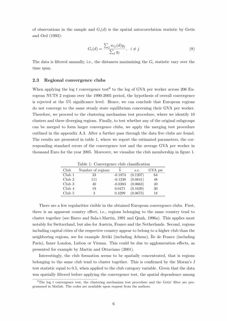
When applying the log t convergence test6 to the log of GVA per worker across 206 Eu-ropean NUTS 2 regions over the 1990-2005 period, the hypothesis of overall convergenceis rejected at the 5% significance level. Hence, we can conclude that European regionsdo not converge to the same steady state equilibrium concerning their GVA per worker.Therefore, we proceed to the clustering mechanism test procedure, where we identify 10clusters and three diverging regions. Finally, to test whether any of the original subgroupscan be merged to form larger convergence clubs, we apply the merging test procedureoutlined in the appendix A.3. After a further pass through the data five clubs are found.The results are presented in table 1, where we report the estimated parameters, the cor-responding standard errors of the convergence test and the average GVA per worker inthousand Euro for the year 2005. Moreover, we visualize the club membership in figure 1.

Table 1: Convergence club classificationClub Number of regions b s.e. GVA pwClub 1 33 -0.1874 (0.1207) 64Club 2 111 -0.1238 (0.0841) 48Club 3 40 -0.0383 (0.0663) 40Club 4 19 0.0471 (0.1639) 30Club 5 3 0.4299 (0.0673) 18

There are a few regularities visible in the obtained European convergence clubs. First,there is an apparent country effect, i.e., regions belonging to the same country tend tocluster together (see Barro and Sala-i-Martin, 1991 and Quah, 1996a). This applies mostnotably for Switzerland, but also for Austria, France and the Netherlands. Second, regionsincluding capital cities of the respective country appear to belong to a higher club than theneighboring regions, see for example Attiki (including Athens), Ile de France (includingParis), Inner London, Lisbon or Vienna. This could be due to agglomeration effects, aspresented for example by Martin and Ottaviano (2001).

Interestingly, the club formation seems to be spatially concentrated, that is regionsbelonging to the same club tend to cluster together. This is confirmed by the Moran’s Itest statistic equal to 0.5, when applied to the club category variable. Given that the datawas spatially filtered before applying the convergence test, the spatial dependence among

6The log t convergence test, the clustering mechanism test procedure and the Getis’ filter are pro-grammed in Matlab. The codes are available upon request from the authors.

6

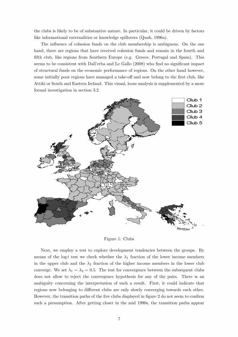
the clubs is likely to be of substantive nature. In particular, it could be driven by factorslike informational externalities or knowledge spillovers (Quah, 1996a).

The influence of cohesion funds on the club membership is ambiguous. On the onehand, there are regions that have received cohesion funds and remain in the fourth andfifth club, like regions from Southern Europe (e.g. Greece, Portugal and Spain). Thisseems to be consistent with Dall’erba and Le Gallo (2008) who find no significant impactof structural funds on the economic performance of regions. On the other hand however,some initially poor regions have managed a take-off and now belong to the first club, likeAttiki or South and Eastern Ireland. This visual, loose analysis is supplemented by a moreformal investigation in section 3.2.

Figure 1: Clubs

Next, we employ a test to explore development tendencies between the groups. Bymeans of the log t test we check whether the λ1 fraction of the lower income membersin the upper club and the λ2 fraction of the higher income members in the lower clubconverge. We set λ1 = λ2 = 0.5. The test for convergence between the subsequent clubsdoes not allow to reject the convergence hypothesis for any of the pairs. There is anambiguity concerning the interpretation of such a result. First, it could indicate thatregions now belonging to different clubs are only slowly converging towards each other.However, the transition paths of the five clubs displayed in figure 2 do not seem to confirmsuch a presumption. After getting closer in the mid 1990s, the transition paths appear

7

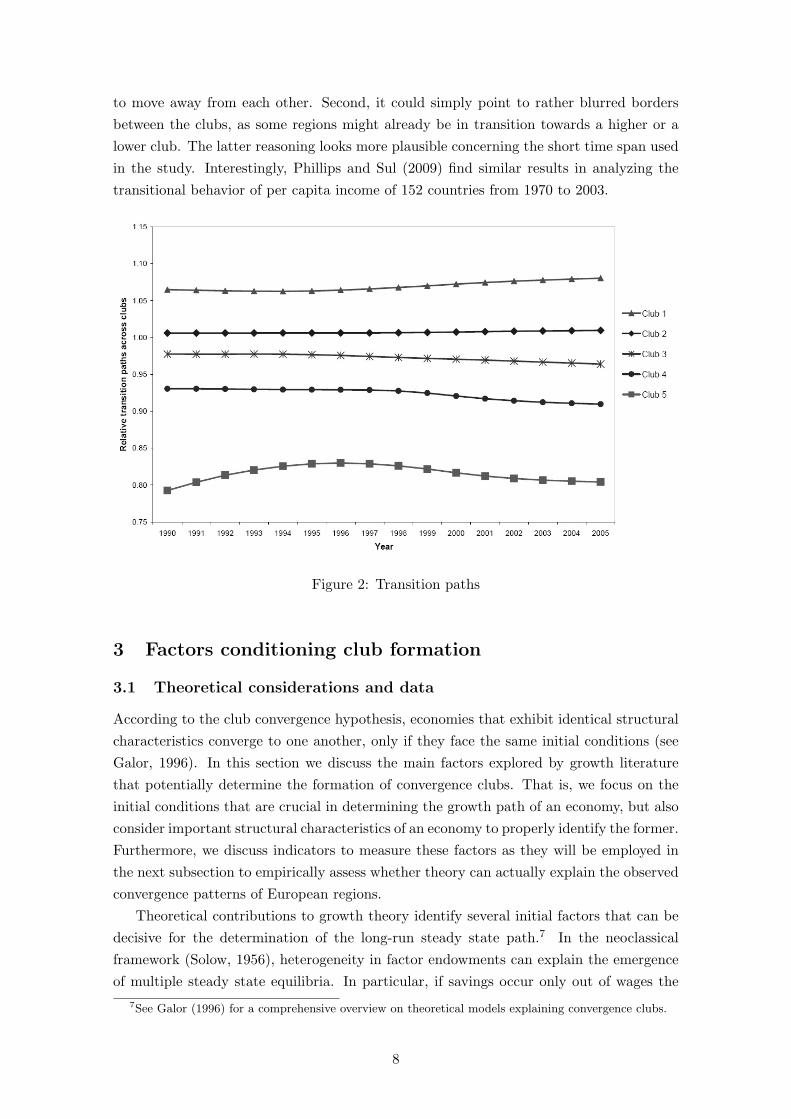
to move away from each other. Second, it could simply point to rather blurred bordersbetween the clubs, as some regions might already be in transition towards a higher or alower club. The latter reasoning looks more plausible concerning the short time span usedin the study. Interestingly, Phillips and Sul (2009) find similar results in analyzing thetransitional behavior of per capita income of 152 countries from 1970 to 2003.

Figure 2: Transition paths

3 Factors conditioning club formation

3.1 Theoretical considerations and data

According to the club convergence hypothesis, economies that exhibit identical structuralcharacteristics converge to one another, only if they face the same initial conditions (seeGalor, 1996). In this section we discuss the main factors explored by growth literaturethat potentially determine the formation of convergence clubs. That is, we focus on theinitial conditions that are crucial in determining the growth path of an economy, but alsoconsider important structural characteristics of an economy to properly identify the former.Furthermore, we discuss indicators to measure these factors as they will be employed inthe next subsection to empirically assess whether theory can actually explain the observedconvergence patterns of European regions.

Theoretical contributions to growth theory identify several initial factors that can bedecisive for the determination of the long-run steady state path.7 In the neoclassicalframework (Solow, 1956), heterogeneity in factor endowments can explain the emergenceof multiple steady state equilibria. In particular, if savings occur only out of wages the

7See Galor (1996) for a comprehensive overview on theoretical models explaining convergence clubs.

8

initial level of the capital-labor ratio can determine which steady state is approached bythe economy (Galor, 1996; Deardorff, 2001). In order to control for differences in factorendowments across regions we employ a labor force variable and use investment datato measure the capital stock of a region. Moreover, to additionally reflect the relativeimportance of factors in production across regions we proxy differences in factor intensitiesby the capital share. Table 2 provides the definition of the variables and the correspondingsources.

Azariadis and Drazen (1990) augment the neoclassical growth model by incorporatingthreshold externalities in the accumulation of human capital that can induce multiple bal-anced growth paths as stationary equilibria. Specifically, due to increasing social returnsto scale that become particularly pronounced when the stock of knowledge attains criticalmass values, the initial conditions with respect to human capital accumulation may deter-mine the growth path of an economy. In particular, the authors argue that rapid growthcan only occur with a relatively overqualified labor force, i.e., a high level of human in-vestment relative to per capita income. To test this presumption, we use the educationalattainment of the working-age population as a proxy for human capital as well as GVAper worker as a measure for per capita income.

To identify the net impact of the initial factors on the formation of convergence clubs,we consider indicators that control for an economy’s structural characteristics. A partic-ularly relevant and often considered prerequisite for a common steady state growth pathof economies is a similar production technology (see for example Galor, 1996). To controlfor differences in production technologies across regions we employ the share of high-techproduction to total service and manufacturing production by relying on the OECD classifi-cation of technology- and knowledge-intensive sectors (see also Mora, 2008). Additionally,we consider the industrial structure of a region by employing GVA in the service sector asa share of total GVA.

Quah (1996a) points to the importance of informational externalities for explainingthe club convergence phenomenon. These externalities may occur either at the state orthe neighborhood level as information is likely to flow more easily across regions thatbelong to the same state or share a border. Indeed, as already discussed in section 2.3(see also Fig.1), European regions belonging to the same country seem to form a commonconvergence club. Also, as reflected by the value of the Moran’s I statistic (i.e., 0.5, seesection 2.3), nearby regions tend to cluster together, indicating that physical location andgeographical spillovers are relevant for the convergence process of European regions. Inorder to capture this form of externality we employ two different indicators. First, we usecountry dummies to control for country membership. Second, we consider the output percapita of neighboring regions to control for geographical spillovers. The idea is that theeconomic activity of a bordering region should influence the own region’s economy andtherefore have an impact on the own regions’s convergence process. More specifically, weuse the spatial lag of GVA per worker, where we apply a contiguity weighting matrix (W )of order one, i.e., regions sharing a border are defined to be neighbors.8

8Note that the neighbor of islands is the region which is the closest in terms of geographical distance.

9

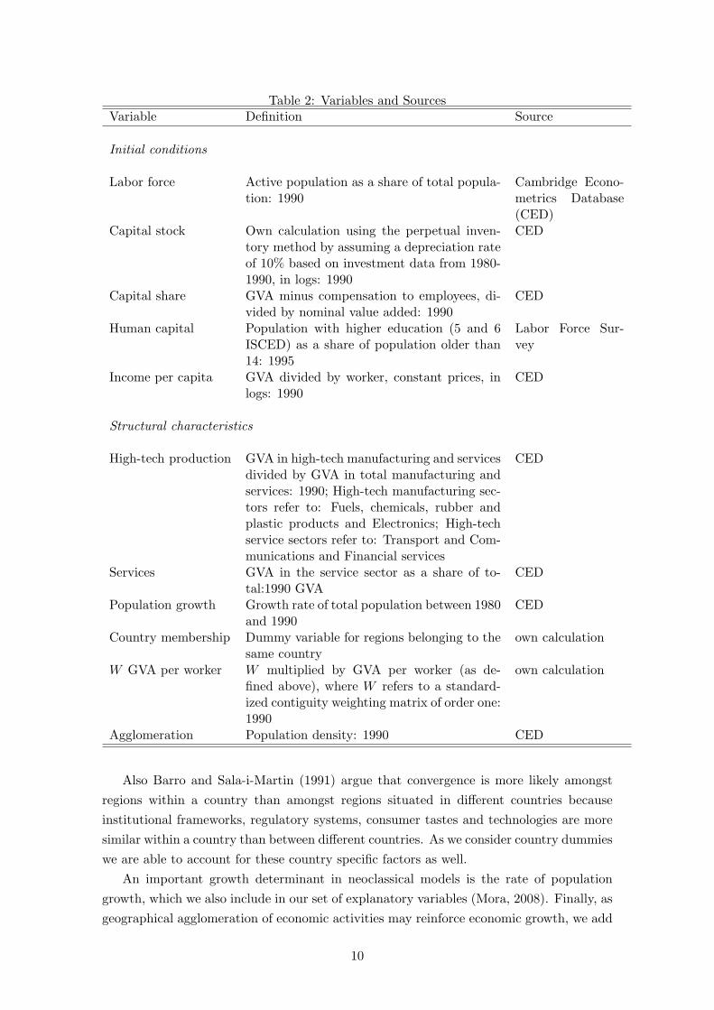
Table 2: Variables and SourcesVariable Definition Source

Initial conditions

Labor force Active population as a share of total popula-tion: 1990

Cambridge Econo-metrics Database(CED)

Capital stock Own calculation using the perpetual inven-tory method by assuming a depreciation rateof 10% based on investment data from 1980-1990, in logs: 1990

CED

Capital share GVA minus compensation to employees, di-vided by nominal value added: 1990

CED

Human capital Population with higher education (5 and 6ISCED) as a share of population older than14: 1995

Labor Force Sur-vey

Income per capita GVA divided by worker, constant prices, inlogs: 1990

CED

Structural characteristics

High-tech production GVA in high-tech manufacturing and servicesdivided by GVA in total manufacturing andservices: 1990; High-tech manufacturing sec-tors refer to: Fuels, chemicals, rubber andplastic products and Electronics; High-techservice sectors refer to: Transport and Com-munications and Financial services

CED

Services GVA in the service sector as a share of to-tal:1990 GVA

CED

Population growth Growth rate of total population between 1980and 1990

CED

Country membership Dummy variable for regions belonging to thesame country

own calculation

W GVA per worker W multiplied by GVA per worker (as de-fined above), where W refers to a standard-ized contiguity weighting matrix of order one:1990

own calculation

Agglomeration Population density: 1990 CED

Also Barro and Sala-i-Martin (1991) argue that convergence is more likely amongstregions within a country than amongst regions situated in different countries becauseinstitutional frameworks, regulatory systems, consumer tastes and technologies are moresimilar within a country than between different countries. As we consider country dummieswe are able to account for these country specific factors as well.

An important growth determinant in neoclassical models is the rate of populationgrowth, which we also include in our set of explanatory variables (Mora, 2008). Finally, asgeographical agglomeration of economic activities may reinforce economic growth, we add

10

population density to our set of explanatory variables to control for agglomerated regions(see e.g. Corrado et al., 2005; Martin and Ottaviano, 2001).

3.2 Results from an ordered probit model

In order to explain the formation of convergence clubs across European regions we employan ordered regression model, first introduced by McKelvey and Zavoina (1975). Thevariable to be explained, denoted by c, indicates the club a region belongs to accordingto the endogenized grouping procedures outlined in section 2.1. As the fifth club consistsof only three regions we pool club 4 and club 5 to one single club, such that c takes onvalues from 1 to 4. This variable can be classified as an ordinal variable since the observedclubs can be ranked according to the steady state per capita income levels of regions inthe respective club but the differences between steady state levels across clubs are notknown. For example, regions belonging to the first club move to a higher income steadystate level than regions belonging to the remaining clubs. Assuming that the membershipin a certain club is related to a continuous, latent variable y∗i that indicates a region’sindividual steady state income level, the model can be written as,

y∗i = Xiβ + εi (9)

where Xi contains the explanatory variables (in the initial period) listed in table 2 aswell as a constant term, with i = 1, ..., 206 indicating the region. The column vector βincludes the structural coefficients. As the dependent variable y∗i is unobserved, the modelcannot be estimated with OLS, but instead Maximum Likelihood (ML) techniques areapplied to compute the probabilities of observing values of c given X (ordered regressionmodel). In order to use ML, the distribution of the error term εi has to be specified. Asis convenient, we assume the errors to be normally distributed with mean 0 and variance1, such that the resulting ordered regression model can be referred to as probit model.Since the latter is non-linear in the probability outcomes, the impact of a variable onthe outcomes can be interpreted in various ways. In order to explore the effect of asingle variable on the probability of belonging to a specific club, we follow the literatureand report marginal effects on probabilities of each variable evaluated at its mean andat the mean of all the other explanatory variables. Furthermore, as we are particularlyinterested in the influence of the initial conditions on the formation of convergence clubs,we display the entire probability curve of each of the initial conditioning variables (giventhey are significant) by holding the remaining variables constant. Hence, we can observethe probabilities of belonging to a certain club depending on the level of the correspondingvariable. 9

In table 3.2 we report marginal effects for each outcome of the club variable c. Atthe bottom of the table we display the number of regions belonging to a particular club,

9For an overview on ordered probit models, see e.g., Greene (2000) and Long (1997). Estimation wasdone by using the command oprobit in Stata.

11

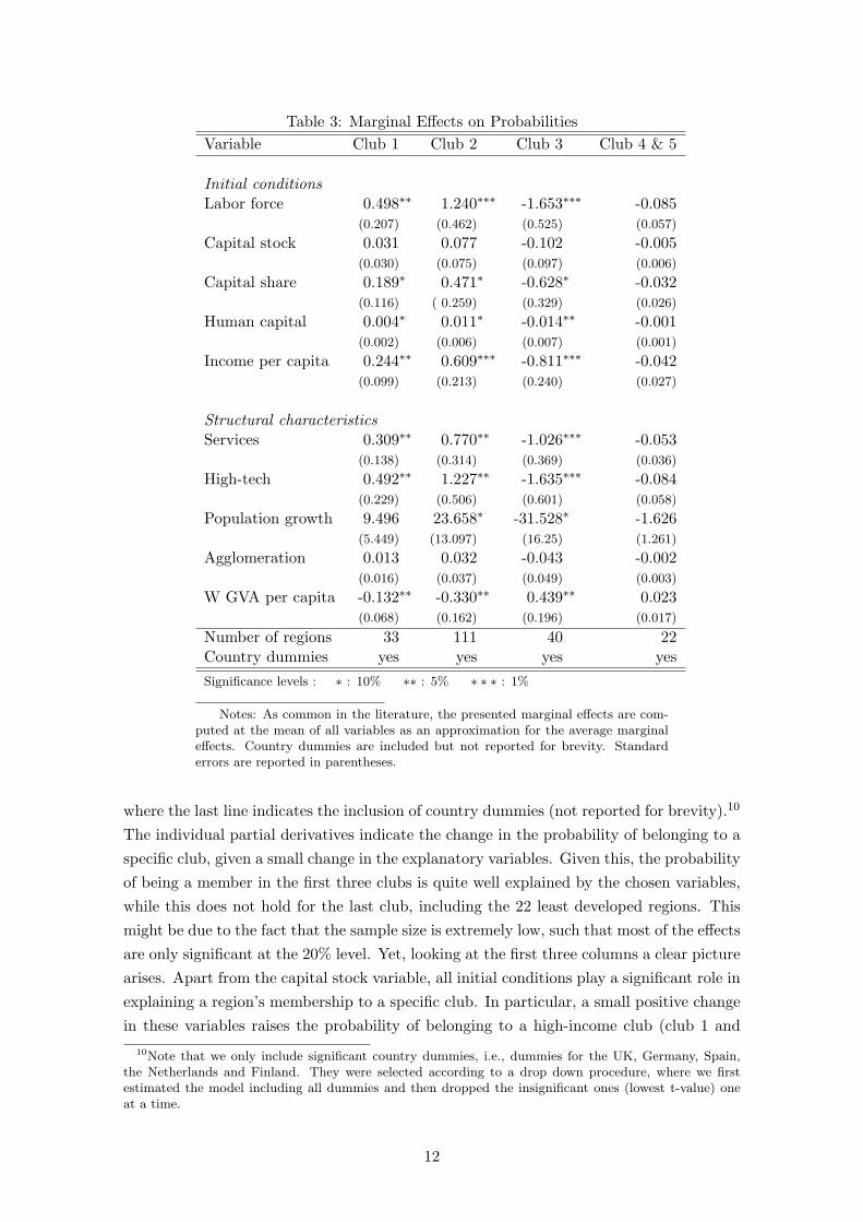
Table 3: Marginal Effects on ProbabilitiesVariable Club 1 Club 2 Club 3 Club 4 & 5

Initial conditionsLabor force 0.498∗∗ 1.240∗∗∗ -1.653∗∗∗ -0.085

(0.207) (0.462) (0.525) (0.057)

Capital stock 0.031 0.077 -0.102 -0.005(0.030) (0.075) (0.097) (0.006)

Capital share 0.189∗ 0.471∗ -0.628∗ -0.032(0.116) ( 0.259) (0.329) (0.026)

Human capital 0.004∗ 0.011∗ -0.014∗∗ -0.001(0.002) (0.006) (0.007) (0.001)

Income per capita 0.244∗∗ 0.609∗∗∗ -0.811∗∗∗ -0.042(0.099) (0.213) (0.240) (0.027)

Structural characteristicsServices 0.309∗∗ 0.770∗∗ -1.026∗∗∗ -0.053

(0.138) (0.314) (0.369) (0.036)

High-tech 0.492∗∗ 1.227∗∗ -1.635∗∗∗ -0.084(0.229) (0.506) (0.601) (0.058)

Population growth 9.496 23.658∗ -31.528∗ -1.626(5.449) (13.097) (16.25) (1.261)

Agglomeration 0.013 0.032 -0.043 -0.002(0.016) (0.037) (0.049) (0.003)

W GVA per capita -0.132∗∗ -0.330∗∗ 0.439∗∗ 0.023(0.068) (0.162) (0.196) (0.017)

Number of regions 33 111 40 22Country dummies yes yes yes yesSignificance levels : ∗ : 10% ∗∗ : 5% ∗ ∗ ∗ : 1%

Notes: As common in the literature, the presented marginal effects are com-puted at the mean of all variables as an approximation for the average marginaleffects. Country dummies are included but not reported for brevity. Standarderrors are reported in parentheses.

where the last line indicates the inclusion of country dummies (not reported for brevity).10

The individual partial derivatives indicate the change in the probability of belonging to aspecific club, given a small change in the explanatory variables. Given this, the probabilityof being a member in the first three clubs is quite well explained by the chosen variables,while this does not hold for the last club, including the 22 least developed regions. Thismight be due to the fact that the sample size is extremely low, such that most of the effectsare only significant at the 20% level. Yet, looking at the first three columns a clear picturearises. Apart from the capital stock variable, all initial conditions play a significant role inexplaining a region’s membership to a specific club. In particular, a small positive changein these variables raises the probability of belonging to a high-income club (club 1 and

10Note that we only include significant country dummies, i.e., dummies for the UK, Germany, Spain,the Netherlands and Finland. They were selected according to a drop down procedure, where we firstestimated the model including all dummies and then dropped the insignificant ones (lowest t-value) oneat a time.

12

Figure 3: Cumulative probability for inititial conditions

club 2), while it decreases the probability of belonging to a low-income club, i.e., club 3.11

Hence, we can conclude that the initial conditions explored by growth theory seem to berelevant in explaining the club formation of European NUTS 2 regions.

Concerning the partial derivatives with respect to the structural characteristics, thesame broad picture arises. Apart from agglomeration, which has an insignificant effect,population growth and both technology variables have the expected positive influence onthe probability of belonging to a high-income club. Interestingly, per worker income ofneighboring regions seems to have a counterintuitive effect on club formation. In partic-ular, an increase in a neighboring region’s income tend to reduce a region’s probabilityof belonging to club 1 and club 2, respectively. Although this is in contrast to expecta-tions, a visual inspection of the map in figure 1 supports the estimation outcome. There,it can be seen that regions belonging to club 1 (mostly metropolitan areas) and club 2are mainly surrounded by regions belonging to a club experiencing lower per worker in-come. This might be the result of backwash effects (Myrdal, 1957), i.e., regions fromhigh-income clubs withdraw resources like labor or capital from their neighbors, where thelatter consequently end up with a lower per worker income.

Finally, we explore how the probability of being a high-income (low-income) regionchanges when we vary the level of the initial conditions. Specifically, we consider eachof the significant variables, i.e., human capital, income per worker, capital share and thelabor force, holding the remaining variables constant. In figure 3 we plot the probabilities

11Note that, the sums of the estimated partial derivatives equal zero across the four clubs because thesums of the probabilities must always equal one.

13

that the outcome is less than or equal to c over the range of values of the respectivevariable, i.e., the probability of at least belonging to club c. For example, the lower line inthe graphs shows the probability of belonging to club 1 when the value of the respectivevariable is altered. In general, all four graphs show the same pattern. The first graphreveals that regions with a high initial endowment of human capital, i.e., 30% of highlyeducated inhabitants, experience a 33% higher probabilitiy (from 0.6 to 0.8) of belongingto a high-income club (club 1 and club 2) than regions with a low initial endowment ofhuman capital (4%). The effect of initial confitions on the probability of converging toclub 1 or 2, is even more pronounced when it comes to per worker income. Regions thatexperienced a low income in the initial period, say 14, 000 Euro, have a probability ofonly 0.08 to at least belong to the second income club, while regions with high per workerincomes, i.e., 67, 000 Euro, show a probabiltiy of 0.98 to converge to a high-income club.Summarizing, we can confirm that it is indeed initial conditions put forward by growththeory (e.g. Azeriadis and Drazen) that determine the path of convergence of Europeanregions’s per worker incomes.

14

4 Conclusion

[to be completed]

Acknowledgments The authors gratefully acknowledge the grant no. P19025-G11 provided

by the Austrian Science Fund (FWF). They thank Manfred M. Fischer for helpful suggestions.

15

A Appendix

A.1 Sample

Our sample includes 206 NUTS 212 regions in 17 countries, covering Austria (nine regions),Belgium (11 regions), Denmark (one region), Finland (five regions), France (22 regions),Western Germany (30 regions), Greece (13 regions), Italy (20 regions), Ireland (two re-gions), Luxembourg (one region), the Netherlands (12 regions), Norway (seven regions),Portugal (five regions), Spain (16 regions), Sweden (eight regions), Switzerland (sevenregions) and the UK (37 regions).

Austria Burgenland; Niederosterreich; Wien; Karnten; Steiermark; Oberosterreich; Salzburg;Tirol; Vorarlberg

Belgium Region de Bruxelles-Capitale/Brussels Hoofdstedelijk Gewest; Prov. Antwer-pen; Prov. Limburg (BE); Prov. Oost-Vlaanderen; Prov. Vlaams-Brabant; Prov.West-Vlaanderen; Prov. Brabant Wallon; Prov. Hainaut; Prov. Liege; Prov. Lux-embourg (BE); Prov. Namur

Denmark Danmark

Finland Ita-Suomi; Etela-Suomi; Lansi-Suomi; Pohjois-Suomi; Aland

France Ile-de-France; Champagne-Ardenne; Picardie; Haute-Normandie; Centre; Basse-Normandie; Bourgogne; Nord - Pas-de-Calais; Lorraine; Alsace; Franche-Comte;Pays de la Loire; Bretagne; Poitou-Charentes; Aquitaine; Midi-Pyrenees; Limousin;Rhone-Alpes; Auvergne; Languedoc-Roussillon; Provence-Alpes-Cote d’Azur; Corse

Germany Stuttgart; Karlsruhe; Freiburg; Tubingen; Oberbayern; Niederbayern; Oberp-falz; Oberfranken; Mittelfranken; Unterfranken; Schwaben; Bremen; Hamburg; Darm-stadt; Gieen; Kassel; Braunschweig; Hannover; Luneburg; Weser-Ems; Dusseldorf;Koln; Mnster; Detmold; Arnsberg; Koblenz; Trier; Rheinhessen-Pfalz; Saarland;Schleswig-Holstein

Greece Anatoliki Makedonia, Thraki; Kentriki Makedonia; Dytiki Makedonia; Thes-salia; Ipeiros; Ionia Nisia; Dytiki Ellada; Sterea Ellada; Peloponnisos; Attiki; VoreioAigaio; Notio Aigaio; Kriti

Italy Provincia Autonoma Bolzano/Bozen & Provincia Autonoma Trento; Piemonte;Valle d’Aosta/Vallee d’Aoste; Liguria; Lombardia; Veneto; Friuli-Venezia Giulia;Emilia-Romagna; Toscana; Umbria; Marche; Lazio; Abruzzo; Molise; Campania;Puglia; Basilicata; Calabria; Sicilia; Sardegna

Ireland Border, Midland and Western; Southern and Eastern

Luxembourg Luxembourg (Grand-Duche)12Nomenclature of Statistical Territorial Units

16

Netherlands Groningen; Friesland; Drenthe; Overijssel; Gelderland; Flevoland; Utrecht;Noord-Holland; Zuid-Holland; Zeeland; Noord-Brabant; Limburg (NL)

Norway Oslo og Akershus; Hedmark og Oppland; Sør-Østlandet; Agder og Rogaland;Vestlandet; Trøndelag; Nord-Norge

Portugal Norte; Algarve; Centro (PT); Lisboa; Alentejo

Spain Galicia; Principado de Asturias; Cantabria; Paıs Vasco; Comunidad Foral deNavarra; La Rioja; Aragon; Comunidad de Madrid; Castilla y Leon; Castilla-LaMancha; Extremadura; Cataluna; Comunidad Valenciana; Illes Balears; Andalucıa;Region de Murcia

Sweden Ostra Mellansverige; Sydsverige; Norra Mellansverige; Mellersta Norrland; OvreNorrland; Smaland med oarna; Vastsverige

Switzerland Region lemanique; Espace Mittelland; Nordwestschweiz; Zurich; Ostschweiz;Zentralschweiz; Ticino

United Kingdom Tees Valley and Durham; Northumberland and Tyne and Wear; Cum-bria; Cheshire; Greater Manchester; Lancashire; Merseyside; East Riding and NorthLincolnshire; North Yorkshire; South Yorkshire; West Yorkshire; Derbyshire andNottinghamshire; Leicestershire, Rutland and Northamptonshire; Lincolnshire; Here-fordshire, Worcestershire and Warwickshire; Shropshire and Staffordshire; West Mid-lands; East Anglia; Bedfordshire and Hertfordshire; Essex; Inner London; OuterLondon; Berkshire, Buckinghamshire and Oxfordshire; Surrey, East and West Sus-sex; Hampshire and Isle of Wight; Kent; Gloucestershire, Wiltshire and North Som-erset; Dorset and Somerset; Cornwall and Isles of Scilly; Devon; West Wales andthe Valleys; East Wales; North Eastern Scotland; Eastern Scotland; South WesternScotland; Highlands and Islands; Northern Ireland

A.2 Clustering algorithm for club convergence identification

If the null hypothesis of the overall convergence is rejected, test for club convergence shouldbe applied, as presented by Phillips and Sul (2007). It consists of the following steps:

Step 1: Cross-section ordering by final observationConvergence, also within clubs, as T →∞ is usually most evident in the final time seriesobservations. The units of the cross-section should be sorted in the descending order dueto the last period in the time series dimension of the panel. In case of significant volatilityin Xit, the sorting can be done according to the time series average over the last 1/2 or1/3 periods of the time dimension.

Step 2: Formation of core group of k∗ regionsTake the first k units (with 2 ≤ k < N) from the panel, run the log t regression. If tb forthis k units is larger than -1.65, add further units one by one and every time calculate tb

17

for the k selected units. Continue as long as the tb is increasing and larger than -1.65 (at5 % significance level). After obtaining a smaller value of tb conclude that the core groupwith k∗ = k − 1 members of a club is formed. If tb > −1.65 does not hold for the firsttwo units, drop the first unit and run the log t regression for the second and third unit.Continue until finding a pair of units with tb > −1.65. If there are no such units in thewhole sample, conclude that there are no convergence clubs in the panel.

Step 3: Sieve the data for new club membersAfter identifying the core group of a club, conduct a test for club membership of otherunits in the panel. Add one of the remaining units at a time to the k∗ members of the coregroup and run the log t regression. Repeat for all the units outside the core group. Selectunits with tb > c, with c being a critical value (c ≥ 0) and add them to the core group.Run the log t test for the whole group. If tb > −1.65, conclude that this group constitutesa convergence club. Otherwise increase the critical value for the club membership selec-tion, form a new group consisting of the core group and all the units with tb larger thanthe increased critical value, and run the log t regression. Repeat till finding tb > −1.65 forthe whole group. Then conclude that those units form a convergence club. If there areno units apart from the core group that result in tb > −1.65, conclude that a convergenceclub consists only of the core group.

Step 4: Recursive and stopping ruleForm a second group from all the units outside the convergence club, i.e., with tb < c. Runthe log t test for the whole group to check whether tb > −1.65 and the group converges. Ifnot, repeat Steps 1-3 on this group to determine whether there is a smaller subgroup thatforms a convergence clubs in the panel. If there is no k in Step 2 for which tb > −1.65,conclude that the remaining units diverge.

A.3 Test for merging

Phillips and Sul (2009) suggest the following test for merging between the groups that areformed according to the clustering algorithm described in appendix A.2: take the first andthe second group and run the log t test, if the t-statistic is larger than -1.65 (5% significancelevel) assume that both groups form a club together, repeat the test after adding the nextgroup, continue until the t-statistic indicates that the convergence hypothesis is rejected.Conclude that all the groups but the last one converge and start the test again from thegroup for which the convergence hypothesis was rejected.

18

References

Anselin, Luc 1988 Spatial Econometrics: Methods and Models. Kluwer, Dordrecht.

Azariadis, Costas, Drazen, Allan 1990. Threshold externalities in economic development.Quarterly Journal of Economic Development 105(2): 501–526.

Barro, Robert J., Sala-i-Martin, Xavier 1991. Convergence across states and regions.Brookings Papers on Economic Activity 22(1): 107–182.

Bernard, Andrew B., Durlauf, Steven N. 1995. Convergence in international output .Journal of Applied Econometrics 10(2): 97–108.

Burkhauser, Richard V., Cutts, Amy Crews, Daly, Mary C., Jenkins, Stephen P. 1999.Testing the significance of income distribution changes over the 1980s business cycle: Across-national comparison. Journal of Applied Econometrics 14(3): 253–272.

Canova, Fabio 2004. Testing for convergence clubs in income per capita: a predictivedensity approach. International Economic Review 45(1): 49–77.

Corrado, Luisa, Martin, Ron, Weeks, Melvyn 2004. Identifying and interpreting regionalconvergence clusters across Europe. Economic Journal 115(502): C133–C160.

Dall’erba, Sandy, Le Gallo, Julie 2008. Regional convergence and the impact of EuropeanStructural Funds over 1989-1999: a spatial econometric analysis. Papers in RegionalScience 87(2): 219–244.

Deardorff, Alan V. 2001. Rich and Poor Countries in Neoclassical Trade and Growth. TheEconomic Journal 111: 277–294.

Desdoigts, Alain 1999. Patterns of economic development and the formation of clubs.Journal of Economic Growth 4(3): 305–330.

Durlauf, Steven N., Johnson, Paul A. 1995. Multiple regimes and cross-country growthbehaviour. Journal of Applied Econometrics 10(4): 365–384.

Galor, Oded 1996. Convergence? Inferences from theoretical models. Economic Journal106(437): 1056–1069.

Getis, Arthur 1995. Spatial filtering in a regression framework: examples using data onurban crime, regional inequality, and government expenditures. In New Directions inSpatial Econometrics, ed. Luc Anselin and Raymond J.G.M. Florax. Springer Verlag,Berlin Heidelberg New York.

Getis, Arthur, Griffith, Daniel A. 2002. Comparative spatial filtering in regression analysis.Geographical Analysis 34(2): 130–140.

Getis, Arthur, Ord, J. Keith 1992. The analysis of spatial association by use of distancestatistics. Geographical Analysis 24(3): 189–206.

19

Greene, William H. 2000 Econometric Analysis. Prentice Hall International, Inc.

Hobijn, Bart, Franses, Philip H. 2000. Asymptotically perfect and relative convergence ofproductivity. Journal of Applied Econometrics 15(1): 59–81.

Hodrick, Rober James, Prescott, Edward C. 1997. U.S. business cycles: an empiricalinvestigation. Journal of Money, Credit and Banking 29(1): 1–16.

Islam, Nazrul 2003. What have we learnt from the convergence debate? Journal of Eco-nomic Surveys 17(3): 309–362.

Long, J. Scott 1997 Regression Models for Categorical and Limited Dependent Variables.Sage Publications, London.

Martin, Philippe, Ottaviano, Gianmarco P. I. 2001. Growth and agglomeration. Interna-tional Economic Review 42(4): 947–968.

McKelvey, Richard D., Zavoina, William 1975. A Statistical model for the analysis ofordinal level dependent variables. Journal of Mathematical Sociology 4: 103–120.

Mora, Toni 2005. Evidencing European regional convergence clubs with optimal groupingcriteria. Applied Economics Letters 12(15): 937–940.

2008. Factors conditioning the formation of European regional convergence clubs. Annalsof Regional Science 42(4): 911–927.

Myrdal, Gunnar 1957 Economic Theory and Underdeveloped Regions. Gerald Duckworth,London.

Phillips, Peter C.B., Sul, Donggyu 2007. Transition modeling and econometric convergencetests. Econometrica 75(6): 1771–1855.

forthcoming. Economic transition and growth. Journal of Applied Econometrics.

Quah, Danny 1996a. Empirics for economic growth and convergence. European EconomicReview 40: 1353–1375.

1996b. Regional convergence clusters across Europe. European Economic Review40: 951–958.

Solow, Robert M. 1956. A contribution to the theory of economic growth. Quarterly Jour-nal of Economics 70(1): 65–94.

20