Regional Assessment of Wind-Powered Desalination Opportunities in the Southwestern U.S.

Prepared for: Larry Flowers National Renewable Energy Laboratory National Wind Technology Center Prepared by: James Androwski, MS student, Department of Environmental Sciences and Policy Abe Springer, Ph.D., Department of Geology Tom Acker, Ph.D., Department of Mechanical Engineering Jan Theron, Ph.D., Department of Mechanical Engineering Grant Brummels, GIS Specialist, Sustainable Energy Solutions Group

June 28, 2007

TABLE OF CONTENTS Page Executive Summary���������������������������... ii Introduction������������������������������... 1 2. GIS Data Categories��������������������������. 1 2.1 Wind Data��������������������������� 2 2.2 Ground Water Data�����������������������.. 2 2.3 Economic Model������������������������.. 3 2.3.1 Capital Costs����������������������. 3 2.3.2 Daily Energy Costs������������������....... 3 3. Conclusions and Recommendations��������������������. 4 3.1 Map Interpretations �����������������������. 4 3.1.1 Wind Resources Map������������������� 4 3.1.2 Predicted Depth to C Aquifer Water Map����������� 4 3.1.3 Predicted TDS of C Aquifer Map��������������. 5 3.1.4 Predicted Depth to C Aquifer Water and Wind Resources Map��.. 5 3.1.5 Predicted TDS of the C Aquifer and Wind Resources Map����. 5 3.1.6 Predicted Capital Costs for a 5 MGD and a 10 MGD Desalination

Plant������������������������... 6 3.1.7 Predicted Energy Costs for a 5 MGD and a 10 MGD Desalination Plants with Co-located Wind Resources ($0.06/kWh)�����.. 6 3.1.8 Predicted Daily Energy Cost for 5 MGD and 10 MGD Desalination Plants Using Grid Electricity ($0.06/kWh and $0.11/kWh)���.. 7 3.2 Assessment of Water Volume�������������������. 7 3.3 Assessment of Report Objectives������������������ 8 3.4 Conclusions and Recommendations����������������� 9 4. References������������������������������. 10 Appendix A: Wind resources for Four Corners Region. Appendix B: Predicted depth to C Aquifer water with labeled data points. Appendix C: Predicted TDS of C Aquifer water with labeled data points. Appendix D: Predicted depth to C Aquifer with wind resources overlay. Appendix E: Predicted TDS of C Aquifer with wind resources overlay. Appendix F: Predicted capital costs for 5 MGD and 10 MGD desalination plants. Appendix G: Predicted daily energy costs using co-located wind resources. Appendix H: Predicted daily energy costs for 5 MGD and 10 MGD desalination plants using

grid electricity at $0.06/ kWh. Appendix I: Predicted daily energy costs for 5 MGD and 10 MGD desalination plants using

grid electricity at $0.11/kWh.

EXECUTIVE SUMMARY There are many areas throughout the U.S. and especially in the west where growth is significant and water resources are strained. In many of these areas, brackish or saline groundwater remains as an unused and potentially valuable resource. These water sources have been unused largely because desalination technologies have historically been energy intensive and therefore have been expensive to implement. However, as water and energy prices continue to increase, there is an opportunity for wind-powered desalination to play a role in meeting the nation�s water needs. To identify locations where wind-powered desalination might be feasible, it is important to understand the geographical distribution of available saline water resources, wind energy, and locations where water consumption is increasing while resources are limited. In this project, we applied the technique we previously developed to display critical wind/desalination related information on Geographical Information System (GIS) maps to the Coconino Aquifer (C Aquifer) of the Colorado Plateau in the Four Corners region. Relevant data sources were identified and entered into ArcGIS to create informative maps. The intended outcome of this study was to provide information sufficient to identify which communities in the region may want to give serious consideration to desalination technologies, and consider supplying the electrical needs of the desalination equipment with wind power Several regional maps were created with a focus on the C Aquifer of the Colorado Plateau: wind resources, GIS interpolated maps showing the depth to- and salinity of- the C Aquifer, and the capital costs and daily energy cost associated with desalination. The C aquifer was chosen in this study because it is known to contain brackish groundwater resources in a region where desalination may be of interest due to growing water demand and limited potable water resources. The U.S. Geological Survey (USGS) was the primary source for water resource information, and NREL for wind energy data. The wind resource map displays 50 m wind power density corresponding to wind classes 1 through 7 in the region. The GIS interpolated maps provide estimates of the spatial distribution of brackish groundwater resources. These interpolated maps were created primarily from well log data maintained in the USGS National Water Information System. The capital cost and daily energy cost maps utilize an economic model to display such costs as a function of the depth to the aquifer, the degree of salinity of the groundwater, and the desalination plant capacity. ArcGIS provides a reasonable interpolation for the depth to the C Aquifer and the TDS concentration in the aquifer were data availability is high and spatially diverse. Areas where actual well log data is unavailable or very limited should be supplemented with interpretive data from the geologic literature to provide a more reasonable interpolation. Such areas include the Hopi Reservation and the northern portion of the Navajo Reservation, and very little groundwater information is available for the C Aquifer in Utah, Colorado, or New Mexico. Good data availability and a reasonable interpolation of this data are found throughout the southern, western, and eastern portions of the study area. The communities this interpolation indicates are located near shallow, saline groundwater resources and wind resources sufficient for electrical generation include Cameron, Leupp, Winslow, Holbrook, Springerville, and Kayenta, Arizona.

ii

For future work we recommend expanding the region of focus to include other principle aquifers of the Colorado Plateau to more fully understand the potential for wind-powered desalination in a region containing stacked, independent aquifers. Other principle water-yielding aquifers in the region as identified by the USGS as containing brackish groundwater resources include the Uinta-Animas aquifer, the Mesa-Verde aquifer, and the Dakota-Glen Canyon aquifer system. We also recommend a creating a site specific conceptual design for a wind-powered desalination plant to more fully understand the costs associated with onshore desalination using wind resources and to evaluate its economic viability in the desert southwest.

iii

INTRODUCTION

Brackish or saline groundwater remains an unused but potentially valuable resource. These water sources have been unused largely because desalination technologies have historically been energy intensive to implement. However, rapid advances in renewable wind energy and desalination have provided a potentially valuable combination of these two technologies. Our previous study developed a technique to display critical wind/desalination related information of a Geographical Information System map that could be used to identify the most promising locations for the potential use of these technologies (Janecek et al., 2005). This project focuses on a regional assessment of wind-powered desalination opportunities within the C aquifer of the Four Corners region including Colorado, Utah, Arizona, and New Mexico. The C aquifer is a multi-aquifer system encompassing Pennsylvanian, Permian, and lower Triassic units of which the Coconino Sandstone and its lateral equivalents, the DeChelly Sandstone and the Glorietta Sandstone, are the principle water-bearing units (Cooley et al, 1969). This assessment includes an estimation of the volume of water available which can be used to determine the sustainability of brackish water supplies as well as an economic model to represent the costs to pump water to the surface and for the treatment of water at various dissolved solid levels. Specific task objectives included:

1. Creating GIS maps that display the potential for desalination in the region of focus, 2. Quantifying the costs of desalination through the formulation of an economic model, and 3. Implementing the economic model in GIS to create maps that display the costs of

desalination (limited capital costs and/or operation and maintenance costs). The intended outcome of this study was to provide information sufficient to identify which communities in the region may want to give serious consideration to desalination technologies, and consider supplying the electrical needs of the desalination equipment with wind power. In the sections that follow, a description is provided for the regional C aquifer depth to water and water salinity maps, the regional wind resource map, and their data sources, then a summary of recommendations and conclusions based on the findings of this research. The final section of the report documents the references used in this project.

2. GIS DATA CATAGORIES

The purpose of this section is to describe the GIS data sources required for the regional desalination map, focused on northeastern Arizona. This portion of Arizona was selected for study because it possesses many of the characteristics typical where desalination may be of interest: growing water demand, lack of abundant potable water resources, and available brackish and saline groundwater resources. Because of the limited resources available to accomplish this project, it was decided early on that the geographic scope of the region must be limited to be thorough in capturing the data required to create the map(s). These maps were created using high resolution wind data acquired from the National Renewable Energy Laboratory and groundwater properties acquired from databases maintained by the USGS and a review of available literature. Additionally, we have included other GIS information such as state and

1

county political boundaries, rivers, and road and highway locations to aid in the interpretation of the GIS maps (U.S. Geological Survey and the University of Arizona, 2005). This section also includes a description of the economic model used to predict the capital costs and the daily energy costs associated with desalinating brackish groundwater.

2.1 WIND DATA The National Renewable Energy Laboratory (NREL) has wind data at two levels of detail (Wind and Hydropower Technologies Program, 2005). The �Wind Power Class� information has been completed for each state and has relatively low detail when compared to the other data source, �Wind Power Density� information. The Wind Power Density maps have been completed for 33 states including Arizona, and have enough detail to show wind power even on ridge-tops and other geographical features. We display the Wind Power Density at 50 meters height for our GIS, but other wind power maps are available for different heights as well as for different seasons. The Wind Power Classes range from 1 to 7, where each class is a representation of a range of wind power densities or equivalent mean wind speeds at a given height (50 m above ground). These classes can serve as an indicator of a region�s wind power development potential. In general, a class 3 wind resource or better is required to develop utility-scale wind power, as would be needed for any large-scale deployment of desalination.

2.2 GROUNDWATER DATA Groundwater data were compiled from a review of numerous ground water reports containing information on the C aquifer. These data are primarily well log data providing location, depth to water, top/bottom elevations for the water-bearing units, and in some cases, water-quality data. 867 well locations were used in this study. The bulk of which (811 well locations) were provided by a numerical groundwater change model created by the USGS to model the effects of groundwater withdrawal on select tributaries of the Little Colorado River (Leake et al., 2005). The USGS has published several other papers evaluating the hydrogeology and water quality of the C aquifer which have provided additional well locations with information on depth to and salinity of the groundwater. Although much of the data are duplicated, several offered pertinent information for additional well locations. A groundwater budget and a general hydrogeologic characterization of the C aquifer were developed by Hart and others (2002) providing depth to water data at an additional 21 well locations. An evaluation of the geology and hydrology of the C aquifer near Leupp, Arizona by Hoffman and others (2005) provided 10 well locations with top/bottom elevations for the water bearing units of the C aquifer. An investigation by the USGS of the hydrogeology of the Mogollon highlands of central Arizona supplied 9 well locations with depth to water information (Parker et al., 2004). A hydrogeological evaluation of the Navajo aquifer in the Greater Aneth Oil Field in San Juan County, Utah provided 5 well locations with depth to water and water salinity data (Spangler et al., 1996). The remaining well locations were found using the online National Water Information System (NWIS) maintained by the USGS. All data acquired from these sources were cross-referenced with the USGS NWIS for the most up to date data for the wells, as well as to add any available water quality data to these locations.

2

Water salinity data on the NWIS are provided as specific conductance (SC). These values were converted to total dissolved solids (TDS) using the general conversion,

TDS = SC x 0.60 x 1000,

where specific conductance is entered in micro-Siemens per centimeter at 25°C and TDS is provided in parts per million (ppm). For the C Aquifer in northern Arizona, the multiplier in this conversion ranges between 0.60-0.80 (US Geological Survey, 2006). Thus by using the 0.60 multiplier, the calculated values reflect minimum values for TDS. 2.3 ECONOMIC MODEL The two-part economic model includes capital costs and energy costs which will be explained in the following subsections. Each of these was implemented in ArcGIS as cost multipliers for the interpolated Predicted Depth to C Aquifer Water and Predicted TDS of C Aquifer layers. 2.3.1 Capital Costs The capital cost estimates are based on the desalination plant capacity (5 and 10 MGD), salinity range, and the cost to drill and outfit a well as a function of the minimum drilling depth required to obtain water from the C Aquifer at any given location. The desalination plants considered are assumed to use reverse osmosis at 300 psi for desalination with some minimal pretreatment of the brackish water feedstock (Mace, et al., 2004). The capital costs include legal and engineering fees with a 35% contingency, but do not include land acquisition, pumping and distribution, water storage, brine disposal, or the capital costs of electrical generation equipment. The desalination plant costs are estimated as $6,062,000 for a 5 MGD desalination plant and $12,827,000 for a 10 MGD desalination plant for desalination of groundwater with a salinity range of 1,000-3,000 ppm TDS. These costs are adjusted upwards by a factor of 1.5 to estimate the additional plant costs for areas with groundwater salinity of 3,000-10,000 ppm TDS. This is a temporary estimate to be used until more accurate values can be acquired. The cost to drill and outfit a well is estimated as $550 per foot of depth to the C Aquifer (pers. Comm. Marvin Glotfelty, 2006). 2.3.2 Energy Costs The energy costs associated with this model include the cost to lift water from the aquifer to the surface and the costs of desalination as a function of plant size and water salinity. The costs of pumping water on maps showing costs to desalinate are estimated by the equation:

(flow rate x TDH x 0.746 x 24 x energy cost)/(3960 x pump efficiency x motor efficiency), where flow rate is in gallons per minute, TDH is the total dynamic head in feet, and energy cost is in $ per kilowatt-hour (pers. Comm. Marvin Glotfelty, 2006). TDH is interpreted from the Predicted Depth to C Aquifer Water map. The energy cost for wind power was estimated at $0.06/kWh. The energy costs using grid electricity were estimated at $0.06/kWh and $0.11/kWh for comparison. Pump efficiency typically ranges from 70%-82% for new equipment and motor

3

efficiency typically ranges from 85%-95% for new equipment (pers. Comm. Marvin Glotfelty, 2006). Mid-range values were used to estimate these parameters, 76% and 90% respectively. The costs of desalination are estimated using values obtained from the Texas Water Development Board (2004) for desalinating water with a salinity range of 1,000-3,000 ppm TDS. The cost of desalination for a 5 MGD plant is $0.79/1,000 gal and for a 10 MGD plant is $0.71/1,000 gal. The costs of desalinating water with a salinity range greater than 3,000 ppm TDS were not considered in this report due to the lack of data on the costs, but these should be included in subsequent work.

3. MAP INTERPRETATIONS AND CONCLUSIONS

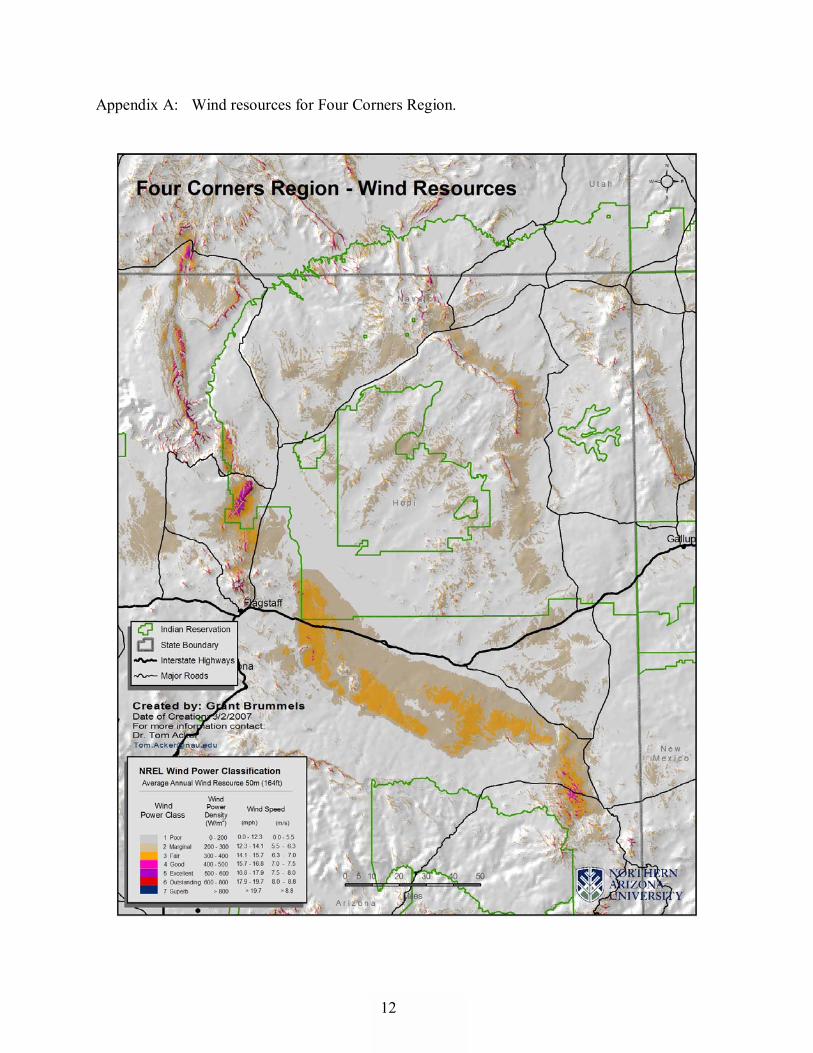
Our map interpretations, conclusions, and recommendations are addressed in the following subsections. Our estimated for water stored in the C Aquifer are addressed in subsection 3.2 � Assessment of Water Volume, and our original report objectives are addressed in subsection 3.3 � Assessment of Report Objectives. 3.1 MAP INTERPRETATIONS Eight GIS maps were produced in this study: wind resources, predicted depth to water, predicted groundwater TDS, estimated capital costs for desalination plants with 5 and 10 MGD capacities, estimated daily energy costs for both 5 and 10 MGD desalination plant capacities utilizing co-located wind resources, and estimated daily energy costs for both 5 and 10 MGD desalination plant capacities utilizing grid electricity at $0.06/kWh and $0.11/kWh. 3.1.1 Wind Resources Map Wind Power Density (50m) data from NREL corresponding to wind classes 1 through 7 were used to create this map which shows regional wind resources (Appendix A). Wind resources are generally found to be poor to marginal (wind class 1 to 2) and are unsuitable for utility-scale electrical generation with current technology. However, wind class generally increases with altitude and sharp changes in topography producing fair to excellent wind resources (wind class 3 to 5) along ridgetops and valley rims both locally and across large areas. Suitable wind fields are oriented along prominent geographical features such as northeastern rim of Black Mesa, and the Gray Mountain Uplift forming the west rim of Little Colorado River valley. The largest such field extends from northwest of Cameron, Arizona on the west rim of the Little Colorado valley southeast to Springerville, Arizona. Small, localized wind fields are found throughout the eastern end of Grand Canyon National Park, Glen Canyon Recreation Area near Page, Arizona, and northwest and southeast of Kayenta, Arizona. 3.1.2 Predicted Depth to C Aquifer Water Map The Kriging method was used in ArcGIS to interpolate the data providing depth to the C Aquifer (Appendix B). This interpolation method provides a reasonable representation of the depth to the aquifer throughout the southern, west central, and east central portions of the study area where data availability is high. These areas include the population centers of Cameron,

4

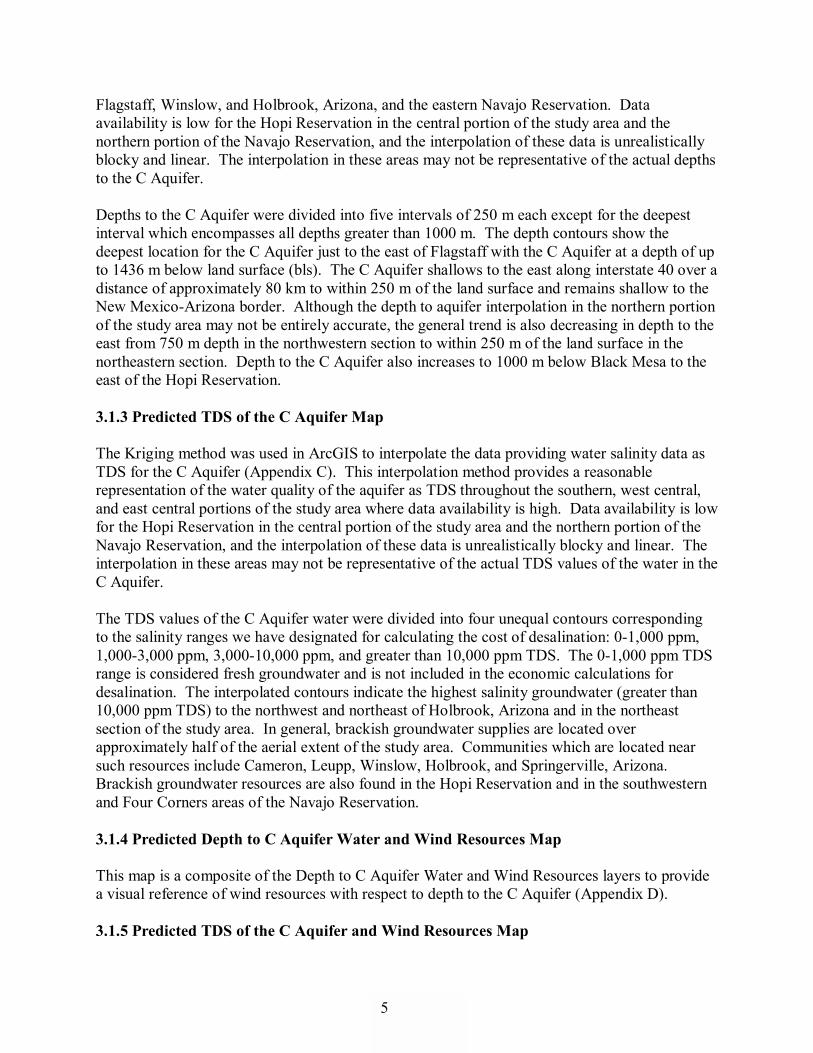
Flagstaff, Winslow, and Holbrook, Arizona, and the eastern Navajo Reservation. Data availability is low for the Hopi Reservation in the central portion of the study area and the northern portion of the Navajo Reservation, and the interpolation of these data is unrealistically blocky and linear. The interpolation in these areas may not be representative of the actual depths to the C Aquifer. Depths to the C Aquifer were divided into five intervals of 250 m each except for the deepest interval which encompasses all depths greater than 1000 m. The depth contours show the deepest location for the C Aquifer just to the east of Flagstaff with the C Aquifer at a depth of up to 1436 m below land surface (bls). The C Aquifer shallows to the east along interstate 40 over a distance of approximately 80 km to within 250 m of the land surface and remains shallow to the New Mexico-Arizona border. Although the depth to aquifer interpolation in the northern portion of the study area may not be entirely accurate, the general trend is also decreasing in depth to the east from 750 m depth in the northwestern section to within 250 m of the land surface in the northeastern section. Depth to the C Aquifer also increases to 1000 m below Black Mesa to the east of the Hopi Reservation. 3.1.3 Predicted TDS of the C Aquifer Map The Kriging method was used in ArcGIS to interpolate the data providing water salinity data as TDS for the C Aquifer (Appendix C). This interpolation method provides a reasonable representation of the water quality of the aquifer as TDS throughout the southern, west central, and east central portions of the study area where data availability is high. Data availability is low for the Hopi Reservation in the central portion of the study area and the northern portion of the Navajo Reservation, and the interpolation of these data is unrealistically blocky and linear. The interpolation in these areas may not be representative of the actual TDS values of the water in the C Aquifer. The TDS values of the C Aquifer water were divided into four unequal contours corresponding to the salinity ranges we have designated for calculating the cost of desalination: 0-1,000 ppm, 1,000-3,000 ppm, 3,000-10,000 ppm, and greater than 10,000 ppm TDS. The 0-1,000 ppm TDS range is considered fresh groundwater and is not included in the economic calculations for desalination. The interpolated contours indicate the highest salinity groundwater (greater than 10,000 ppm TDS) to the northwest and northeast of Holbrook, Arizona and in the northeast section of the study area. In general, brackish groundwater supplies are located over approximately half of the aerial extent of the study area. Communities which are located near such resources include Cameron, Leupp, Winslow, Holbrook, and Springerville, Arizona. Brackish groundwater resources are also found in the Hopi Reservation and in the southwestern and Four Corners areas of the Navajo Reservation. 3.1.4 Predicted Depth to C Aquifer Water and Wind Resources Map This map is a composite of the Depth to C Aquifer Water and Wind Resources layers to provide a visual reference of wind resources with respect to depth to the C Aquifer (Appendix D). 3.1.5 Predicted TDS of the C Aquifer and Wind Resources Map

5

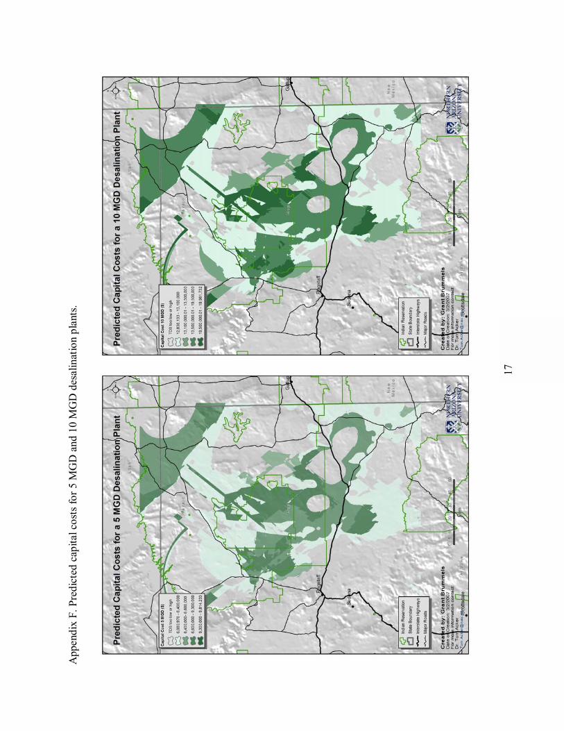
This map is a composite of the TDS of the C Aquifer and Wind Resources layers to provide a visual reference of wind resources with respect to salinity of the C Aquifer (Appendix E). 3.1.6 Predicted Capital Costs for a 5 MGD and a 10 MGD Desalination Plant These estimated capital costs are based on the desalination plant capacity (5 and 10 MGD), salinity range, and the cost to drill and outfit a well (Appendix F). The Depth to C Aquifer layer was cropped by the TDS layer to only include the salinity ranges of 1,000-3,000 ppm and 3,000-10,000 ppm TDS. All depths within this area were multiplied by estimations of the previously mentioned characteristics for capital costs as outlined in section 2.3.1. The capital costs range from $6,400,000 to $9,800,000 for the 5 MGD desalination plant and $12,800,000 to $20,000,000 for the 10 MGD desalination plant. On both maps these costs were divided into four unequal contours. The highest costs are associated with locations were groundwater is deepest and/or the most saline. Such locations include south of Winslow, Arizona, the Hopi Reservation, and the southern, western, and Four Corners areas of the Navajo Reservation. The lowest cost areas are in the central portion of the study area including Kayenta, Arizona and the northern end of the Hopi Reservation and in the southern portion of the study area near Winslow, Holbrook, and Springerville, Arizona. Although some interpretation is made for locations in the central and northern portions of the study area, these interpretations are made with only minimal confidence due to the limited data availability in these areas as described in sections 3.1.2 and 3.1.3. 3.1.7 Predicted Energy Costs for 5 MGD and 10 MGD Desalination Plants with Co-located Wind Resources ($0.06/kWh) These maps are derived by using the salinity contour for the 1,000-3,000 ppm TDS range to crop the wind resources data thereby showing only the locations which contain groundwater with 1,000-3,000 ppm TDS and wind class 3 or better (Appendix G). These locations were multiplied in ArcGIS by our Energy Costs economic model as described in section 2.3.2 to yield estimated costs associated with lifting and desalinating water from the C Aquifer using co-located wind resources. The daily energy costs predicted by this model range from $1,105-$5,120 for the 5 MGD plant and $2,209-$10,241 for a 10 MGD plant. The difference in costs between the two plants considered reflects a doubling in the amount of water being produced. The highest costs on either map are associated with the highest salinities and the greatest depths to the aquifer. On both maps these costs were divided into four unequal contours. Four areas are identified as containing both brackish groundwater and sufficient wind resources: Leupp, Arizona, south of Winslow and Holbrook, Arizona, northwest of Springerville, Arizona, and southeast of Kayenta, Arizona. There are also a scattering of isolated hilltops and ridges throughout the Navajo and Hopi reservations which may provide these resources characteristics.

6

Although some interpretation is made for locations in the central and northern portions of the study area, these interpretations are made with only minimal confidence due to the limited data availability in these areas as described in sections 3.1.2 and 3.1.3. 3.1.8 Predicted Daily Energy Cost for 5 MGD and 10 MGD Desalination Plants Using Grid Electricity ($0.06/kWh and $0.11/kWh) These maps were derived using all locations which contain groundwater with 1,000-3,000 ppm TDS and are not limited to areas with sufficient wind resources (Appendices H and I). These locations were multiplied in ArcGIS by our Energy Costs economic model as described in section 2.3.2 to yield estimated costs associated with lifting and desalinating water from the C Aquifer using grid electricity. Neither the proximity to current electrical transmission equipment nor the costs of new such equipment are considered in this report. For these purposes, it is assumed that electricity is available anywhere it may be needed. The daily energy costs predicted by this model at $0.06/kWh range from $1,377-$4,129 for the 5 MGD plant and from $2,754-$8,259 for the 10 MGD plant. The daily energy costs predicted by this model at $0.11/kWh range from $2,524 to $7,570 for the 5 MGD plant and from $5,049-$15,141 for the 10 MGD plant. The difference in costs between the two plants considered at either energy cost rate reflects a doubling in the amount of water being produced. The highest costs on all maps are associated with the highest salinities and the greatest depths to the aquifer. On all of these maps the costs were divided into four unequal contours. In general, the highest cost locations are found near the interpolated 3,000-10,000 ppm TDS contour. At many locations the cost grades from the highest to the lowest cost over a very short distance, less than 10 km. Although some interpretation is made for locations in the central and northern portions of the study area, these interpretations are made with only minimal confidence due to the limited data availability in these areas as described in sections 3.1.2 and 3.1.3. 3.2 ASSESSMENT OF WATER VOLUME Estimates for the volume of water stored in the C Aquifer are dependent on the hydrogeologic properties of the rock unit. The Coconino Sandstone is the principle water-yielding rock unit of the C Aquifer. The hydrological properties of this unit vary greatly across its extent due to varying degrees of fracturing, differences in the penetration depths of wells used in aquifer tests, and variations inherent to the unit (Leake et al., 2005). The C Aquifer contains both confined and unconfined areas, but has been determined to act as if it were unconfined or �semi-confined� in response to pumping. For the purposes of a general estimate, we assume the C Aquifer is unconfined although, it is known to be confined by the Moenkopi Formation in the northern and eastern portions of its extent. The amount of water that an unconfined aquifer can hold per unit area per unit change in hydraulic head is calculated using the equation for storativity (S). S = Sy + bSs,

7

where Sy is the specific yield, b is aquifer thickness, and Ss is the specific storage. The aquifer thickness ranges from 91 m to 637 m with an average of 119 m (Leake et al, 2005). Specific yield, 0.06, and specific storage, 6.56 x 10-6 m-1, are based on aquifer tests conducted near Leupp, Arizona (Hoffman et al, 2005). The storativity based on the average aquifer thickness is calculated at 0.0608. This unit is dimensionless, but represents the volume of water that is released (or taken into) storage per unit change in hydraulic head for a given area. If the hydraulic head change is assumed to be one meter and the unit area considered is one square meter, then the C Aquifer may yield on average 0.06 m3 of water per square meter of the aquifer for every 1 m drop in the water level. This GIS calculated 284,638 200 m x 200 m cells or an area covering 11 x 109 m2 within the C Aquifer as containing water with a salinity of 1,000-3,000 ppm TDS. This yields an estimated 692 x 106 m3 water in storage for every 1 m drop in water level. Total water in storage is estimated at 82 x 109 m3. 3.3 ASSESSMENT OF REPORT OBJECTIVES Objective 1 � Create GIS maps that display potential for desalination in region of focus: The most relevant layers in this GIS model include wind resources, depth to the C Aquifer, salinity levels, and the costs of desalination as displayed on the various maps in the Appendices. Other information such as roads, highways, cities, and state and tribal political boundaries are also included to aid in the interpretation of the maps. ArcGIS was used to interpolate the regional distribution of brackish groundwater and the depths to the C Aquifer from specific well log data, but our opinion on the degree of uncertainty in the interpolation is dependent on the spatial diversity of the data. High data availability over a large region provides a reasonable interpolation of the data, but areas with concentrated data points or no data provide only speculative information at best. The aerial extent of the study area as shown on the maps in the Appendices are thus smaller than the regional extent of the C Aquifer due to limited availability of well log data in this aquifer outside of northeastern Arizona. Additional data points will be required either from well logs or from geologic interpretations in the scientific literature to smooth the interpolation in these areas. Objective 2 � Quantify the costs of desalination through formulation of an economic model: The capital costs and daily energy costs were estimated as outlined in subsections 2.3.1 and 2.3.2. Cost values were included for 1, 5, and 10 MGD desalination plants with the capacity to desalinate water with salinity of 1,000-3,000 ppm TDS. Only a rough estimate of the costs to desalinate water with salinity greater than 3,000 ppm TDS is provided. Additional cost values are needed to better estimate the capital costs in areas where groundwater salinity is in excess of 3,000 ppm TDS. The capital costs also only consider the costs associated with well and desalination equipment and should include the capital costs associated with electrical generation where co-located wind is available or electrical transmission where wind power is not available. Objective 3 � Implement economic model in GIS to create maps that can display costs of desalination (limited capital costs and/or operation and maintenance costs): The economic model was successfully implemented in GIS to produce the Predicted Cost maps as described in subsections 3.1.6-3.1.8 and presented in the Appendices. The estimated costs are dependent on- and only as good as- the GIS interpolations for the Predicted Depth to the C Aquifer and the Predicted TDS of the C Aquifer layers. Data for these layers provided a

8

reasonable interpolation generally throughout the western, southern, and eastern portions of the study area, but require additional data as described in Assessment of Objective 1. 3.4 CONCLUSIONS AND RECOMMENDATIONS ArcGIS provides a reasonable interpolation for the depth to the C Aquifer and the TDS concentration in the aquifer were data availability is high and spatially diverse. Fortunately, this occurs near community centers, because these are the areas where groundwater exploration has been conducted. Areas where actual well log data is unavailable should be supplemented with interpretive data from the geologic literature to provide a more reasonable interpolation. Communities which are found to be located near shallow, saline groundwater resources and wind resources sufficient for electrical generation include Cameron, Leupp, Springerville, and Kayenta, Arizona. Brackish groundwater resources are also found south of Winslow and Holbrook, on the Hopi Reservation, and in the southern and Four Corners region of the Navajo Reservation. The interpolation of the groundwater resources on the Hopi Reservation and in the Four Corners region of the Navajo Reservation is speculative due to insufficient data, but the interpolation suggests that these areas should contain moderately- to highly-brackish groundwater at relatively shallow depths. While this GIS indicates these communities may wish to consider wind-powered desalination due to the proximity of resources, our judgment for warranted appraisal studies lacks the detailed community information that the communities themselves have, and therefore, we do not recommend making judgments of warranted appraisal studies using this GIS. We emphasize the purpose of this GIS is strictly to provide enough information for communities to make their own judgments whether an appraisal study is warranted. The costs associated with our economic model are still being developed and should be considered only as general estimates. We recommend creating a site specific conceptual design for a wind-powered desalination plant to more fully understand the costs associated with the integration of wind-powered electrical generation and desalination technology and to evaluate its economic feasibility. Some other questions that such a study may address are whether the electrical generation and desalination equipment should be co-located or if one could develop them in separate places and connect them through the utility grid. Also of interest is to understand if there is any potential to run desalination equipment (e.g., reverse osmosis) directly from wind energy, or if grid-quality AC electricity is required. The C Aquifer is one of several aquifers in a �stacked-aquifer system� on the Colorado Plateau such that any location of the Colorado Plateau may have access to one or more aquifers within this system. To more thoroughly understand the potential for wind-powered desalination in the southwestern U.S., we recommend expanding the region of focus in subsequent studies to include other principle water-yielding aquifers such as the Uinta-Animas aquifer, the Mesa-Verde aquifer, and the Dakota-Glen Canyon aquifer system. These aquifers have been identified by the USGS as being regional in extent and containing brackish groundwater resources. These aquifers may provide such resources where the C Aquifer of this study does not or at a lesser cost.

9

REFERENCES Bills, D. J. and M. E. Flynn, 2002, Hydrogeologic data for the Coconino Plateau and adjacent

areas, Coconino and Yavapai Counties, Arizona: US Geological Survey Open-File Report 02-265.

Cooley, M. E., J. W. Harshbarger, J. P. Akers, and W. F. Hardt, 1969, Regional hydrology of the

Navajo and Hopi Indian Reservations, Arizona, New Mexico, and Utah: US Geological Survey Professional Paper 521-A.

Glotfelty, M., 2006, personal communication, 20 October 2006. Hart, R. J., J. J. Ward, D. J. Bills, and M. E. Flynn, 2002, Generalized hydrogeology and ground-

water budget for the C aquifer, Little Colorado River Basin and parts of the Verde and Salt River Basins, Arizona and New Mexico: U.S. Geological Survey Water-Resources Investigations Report 02-4026.

Hoffman, J. P., D. J. Bills, J. V. Phillips, and K. J. Halford, 2005, Geologic, hydrologic, and

chemical data from the C aquifer near Leupp, Arizona: U.S. Geological Survey Scientific Investigation Report 2005-5280.

Janecek, J., T. Acker, A. Springer, J. Theron, M. Malone, G. Brummels, S. Martin, 2005,

Mapping approach to wind desalination opportunities in the U.S.: Northern Arizona University, Flagstaff, Arizona, unpublished.

Leake, S. A., J. P. Hoffman, and J. E. Dickinson, 2005, Numerical ground-water change model

of the C aquifer and effects of ground-water withdrawals on stream depletion in selected reaches of Clear Creek, Chevelon Creek, and the Little Colorado River, northeastern Arizona: U.S. Geological Survey Scientific Investigations Report 2005-5277.

Mace, R.E., E.S. Angle, and W.F. Mullican III, Editors, 2004, Aquifers of the Edwards Plateau:

Texas Water Development Board Report 360. Parker, J. T. C., W. C. Steinkampf, and M. E. Flynn, 2004, Hydrology of the Mogollon

Highlands of central Arizona: U.S. Geological Survey Scientific Investigations Report 2004-5294.

Spangler, L. E., D. L. Naftz, and Z. E. Peterman, 1996, Hydrology, chemical quality, and

characterization of salinity in the Navajo aquifer in and near the Greater Aneth Oil Field, San Juan County, Utah: U.S. Geological Survey Water-Resources Investigations Report 96-4155.

US Geological Survey, 2006, Correspondence with staff at Flagstaff Field Station, Flagstaff,

Arizona. U.S. Geological Survey and the University of Arizona, 2005, Southern Arizona Data Services

Program, information from website: http://sdrsnet.srnr.arizona.edu/index.php

10

Wind and Hydropower Technologies Program, 2005, Wind Power Class and Wind Power

Density GIS information from website: http://www.eere.energy.gov/windandhydro/windpoweringamerica/wind_maps.asp

11

Appendix A: Wind resources for Four Corners Region.

12

Appendix B. Predicted depth to C Aquifer water with labeled data points.

13

Appendix C: Predicted TDS of C Aquifer water with labeled data points.

14

Appendix D: Predicted depth to C Aquifer with wind resources overlay.

15

Appendix E: Predicted TDS of C Aquifer with wind resources overlay.

16

App

endi

x F.

Pre

dict

ed c

apita

l cos

ts fo

r 5 M

GD

and

10

MG

D d

esal

inat

ion

plan

ts.

17

App

endi

x G

. Pre

dict

ed d

aily

ene

rgy

cost

s of d

esal

inat

ion

usin

g co

-loca

ted

win

d re

sour

ces a

t $0.

06/k

Wh.

18

App

endi

x H

. Pre

dict

ed d

aily

ene

rgy

cost

s for

5 M

GD

and

10

MG

D d

esal

inat

ion

plan

ts u

sing

grid

ele

ctric

ity a

t $0.

06/ k

Wh.

19

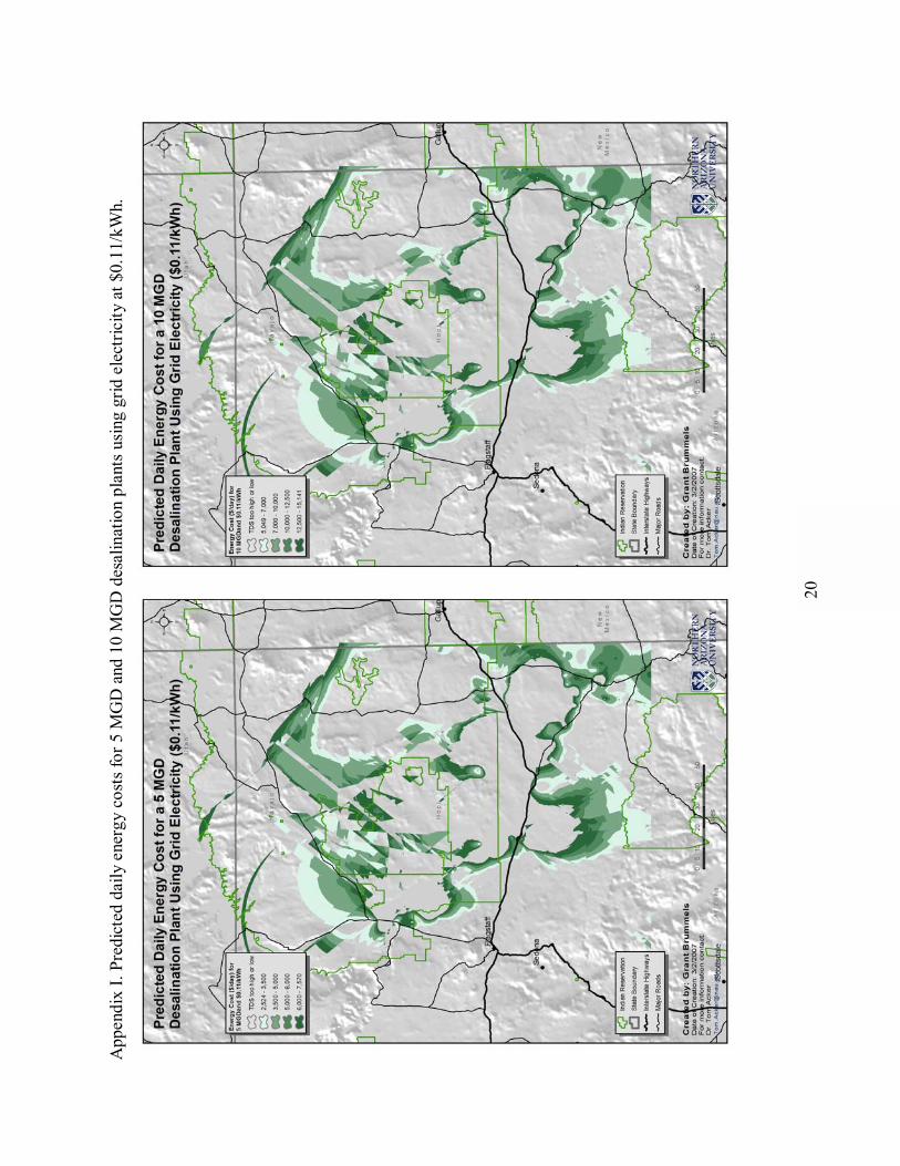
App

endi

x I.

Pred

icte

d da

ily e

nerg

y co

sts f

or 5

MG

D a

nd 1

0 M

GD

des

alin

atio

n pl

ants

usi

ng g

rid e

lect

ricity

at $

0.11

/kW

h.

20