references - springer978-1-4757-3304-4/1.pdf · empirical software engineering 1996, 1(2): 133-164....
TRANSCRIPT

REFERENCES Agarwal R, De P, Sinha AP. Comprehending Object and Process Models: An Empirical Study. IEEE Transactions on Software Engineering 1999; 25 (4): 541-555.
Alston WP. Philosophy of Social Sciences. Foundation in Philosophy Sciences. New Jersey: Prentice Hall, 1966.
Anderson VL; McLean RA. Design C?f Experiments: A Realistic Approach. New York: Marcel Dekker Inc, 1974.
Arisholm E, Sjoberg D. Empirical Assessment of Changeability. Proceedings of the ICSE '99 Workshop; 1999 May 18; Los Angeles, USA: 62-69
Basili VR, Caldiera G, Rombach HD. "The GQM approach". In the Encyclopedia of Software Engineering, Wiley, 1994.
Basili VR, Reiter RW Jr. A Controlled Experiment Quantitatively Comparing Software Development Approaches. IEEE Transactions on Software Engineering 1981; 7 (3): 299-320.
Basili VR, Selby RW. Comparing the Effectiveness of Software Testing Strategies. IEEE Transactions on Software Engineering 1987; 13 (12): 1278-1296.
Basili VR, GreenS, Laitenberger 0, Lanubile F, Shull F, Sorumgard S, Zelkowitz MY. The Empirical Investigation of Perspective-Based Reading. Empirical Software Engineering 1996, 1(2): 133-164.
Basili VR, Lanubile F, Shull F. Investigating Maintenance Processes in a Framework-Based Environment. Proceedings of the International Conference on Software Maintenance {ICSM '98); Bethesda, Maryland, IEEE Computer Society Press, 1998: 256-264.
Basili V, Shull F, Lanubile F. Building Knowledge through Families of Experiments. IEEE Transactions on Software Engineering 1999; 25 (4): 456-473.
Box G, Hunter W, Hunter J. Statistics for Experimenters. An Introduction to Design Data Analysis and Model Building. New York: John Wiley & Sons, 1978.
Briand L, El Emam K, Morasca S. On the Application of Measurement Theory in Software Engineering. Empirical Software Engineering 1996; I: 61-88.
Briand LC, El Ernam K, Freimut B, Laitenberger 0. Quantitative Evaluation of Capture-Recapture Models to Control Software Inspections. Proceedings of the Eighth International Symposium on Software Reliability Engineering 1997; Albuquerque. Los Alamitos: IEEE Comput. Soc., 1997.
Briand LC, Bunse C, Daly J W, Differding C. An Experimental Comparison of the Maintainability of Object-Oriented and Structured Design Documents. Empirical Software Engineering 1997; 2: 291-312.
Brown RW, Lennenberg EH. A Study in Language and Cognition. Journal of Abnormal and Social Psychology 1954; 49: 454-462.

360 References
Browne JC, Lee T, Werth J. Experimental Evaluation of a Reusability-Oriented Parallel Programming Environment. IEEE Transactions on Software Engineering 1990; 16 (2): 111-120.
Campbell DT, Stanley JC. Experimental and Quasi-Experiental Designs for Research. Boston MA: Boughton Mifflin Company, 1963.
Cartwright M, Shepperd MJ. An Empirical View oflnheritance. Infonnation and Software Technology 1998; 40 (14): 795-799.
Cohen D. The Secret Language of the Mind. London: Duncan Baird Publishers, 1996.
Cook TO, Campbell DT. Experimental and Quasi-Experienta/ Designs for Research. Boston MA: Boughton Mifflin Company, 1979.
Counsell S, Newson P, Harrison R. Use of Friends in C++ Software: An Empirical Investigation. Proceedings of the International Conference on Software Engineering; 1999 May 18; Los Angeles, USA: 70-74.
Cronbach U, Meehl PE. Construct validity in psychological tests. Psychological Bulletin 1955; 5: 281-303.
Daly A, Brooks A, Miller J, Roper M, Wood M. An External Replication of a Korson Experiment. Technical Report Empirical Foundations of Computer Science EFoCS-4-94, Departmet of Computer Science, University ofStrathclyde, Glasgow, 1994.
Daly A, Brooks A, Miller J, Roper M, Wood M. The Effect of Inheritance on the Maintainability of Object-Oriented Software: En Empirical Study. Proceedings of the International Conference on Software Maintenance, 1995. Los Alamitos: IEEE Comput. Soc. Press, 1995.
Duncan DB. Multiple Range and Multiple F Test. Biometrics 1955; II: 1-42.
Ebert C. Experiences with Criticality Predictions in Software Development. Proceedings of the 6th ESEC, held Jointly with the 5th ACM SIGSOFTS Symposium on the FSE; 1997 September; Zurich, Switzerland. Software Engineering Notes 1997; 22 (6): 278-293.
Ebert C. The Road to Maturity: Navigating Between Craft and Science. IEEE Software, 1997; November/December: 77-82.
Ericson KA, Simon HA. Protocol Analysis: Verbal Reports as Data. Cambridge: MIT Press, 1984.
Fenton N, Pfleeger SL, Glass RL. Science and Substance: A challenge to software engineers. IEEE Software 1994; July: 86-95.
Fenton N, Pfleeger SL. Software Metrics: A Rigorous & Practical Approach. 200 Edition. Boston, MA: PWS Publishing Company, 1997.
Fox H. The Legacy of Cold Fusion, Truth, History and Status. New Enginery News, 1997; 5 (5): 4-5.
Fusaro P, Lanubile F, Visaggio G. A Replicated Experiment to Assess Requirements Inspection Techniques. Empirical Software Engineering 1997; 2: 39-57.

Basics of Software Engineering Experimentation 361
Gibbons JD, Chakraborti S. Nonparametric statistical inference. 3n1 Edition. New York : Marcel Dekker, 1992
Glass GV, McGraw B, Smith ML. Meta-analysis in Social Research. Beverly Hills, CA: SAGE, 1981.
Harrison R, Samaraweera LG, Dobie MR, Lewis PH. Comparing programming paradigms: an evaluation of functional and object-oriented programs. Software Engineering Journall996; July: 247-254.
Hatton L. Does 00 Really Match the Way We Think?, IEEE Software 1998; May: 46-54.
Houdek F, Ernst D, Schwinn T. Comparing Structured and Object-Oriented Methods for Embedded Systems: A Controlled Experiment. Proceedings of the ICSE '99 Workshop; 1999 May 18; Los Angeles.
Judd CM, Smith ER, Kidder LH. Research Methods in Social Relations. Orlando, Florida: Harcourt Brace Jovanovich College Publishers, 1991.
Kamsties E, Lott CM. An empirical evaluation of three defect detection techniques. Technical Report International Software Engineering Research Network ISERN-95-02, Department of Computer Science University of Kaiserlautern, May 1995.
Kitchenham B. Software Metrics. Oxford: Blackwell Publishers Inc., 1996.
Korson TD, Vaishnavi UK. An empirical study ofthe effects of modularity on program modificability. Proceedings of the First Workshop on Engineering Studies of Programmers; 1986. Ablex Publishig Corporation, 1986.
Laitenberger 0, DeBaud J-M. Perspective-based reading of code documents at Robert Bosch GmbH. Information and Software Technology 1997; 39: 781-791.
Land LPW, Sauer, C, Jeffery R. Validating the Defect Detection Performance Advantage of Group Designs for Software Reviews: Report of a Laboratory Experiment Using Program Code. Proceedings of the 6th ESEC, held jointly with the 5th ACM SIGSOFTS Symposium on the FSE; 1997 September; Zurich, Switzerland. Software Engineering Notes 1997; 22 (6): 294-309.
Latour B, Woolgor D. Laboratory Life. The Construction of Schence Facts. Princenton, USA: Princenton University Press, 1986.
Lennenberg EH. Cognition in Ethnolinguistics. Language 1953; 29: 463-471.
Lewis JA, Henry SM, Kafura DG, Schulman RS. An Empirical Study of the Object-Oriented Paradigm and Software Reuse. SIGPLAN-Notices 1991; 26 (II): 184-96.
Lewis JA, Henry SM, Kafura DG, Schulman RS. On the Relationship between the Object Oriented Paradigm and Software Reuse: An Empirical Investigation. Journal of Object Oriented Programming 1992; July/ August: 35-41.
Lott CM, Rombach HD. Repeatable Software Engineering Experiments for Comparing DefectDetection Techniques. Empirical Software Engineering 1996; 1: 241-277.

362 References
Macdonald F, Miller J. A Comparison of Tool-Based and Paper-Based Software Inspections. Technical Report International Software Engineering Research Network ISERN-98-17, Department of Computer Science, University ofStrathclyde, UK, 1998.
Maibaum T. What We Teach Software Engineers in the Unviersity: Do We Take Engineering Seriosuly?. Proceedings of the ESEC/FSE, 1997. Software Engineering Notes, 1997,22 (6}: 40-50.
Matos V, Jalics P-J. An Experimental Analysis of the Performance of Fourth-Generation Tools on PCs. Communications of ACM 1989; 32 (II): 1340-1350.
Miles MB, Huberman AM. Qualitative Data Analysis, 2nd Edition. London: Sage Publications, 1994.
Miller J, Daly J, Wood M, Roper M, Brooks A. Statistical Power and its subcomponents- missing and misunderstood concepts in empirical software engineering research. Journal of Information and Software Technology, 1997; 39 (4): 285-295.
Misra SK Jalics PJ. Third-Generation versus Fourth-Generation Software Development. IEEE Software 1988; July: 8-14.
Mizuno 0, Kikuno T, lnagaki K, Takagi Y, Sakamoto K. Analyzing Effects of Cost Estimation Accuracy on Quality and Productivity. Proceedings of the 20th International Conference on Software Engineering (ICSE'98); 1998 Aprill9- 25; Kyoto. Los Alamitos: IEEE Comput. Soc, 1998.
Mizuno 0, Kikuno T. Empirical Evaluation of Review Process Improvement Activities with respect to Post-Release Failure. Proceedings of the 21th International Conference on Software Engineering (ICSE'98); 1999 May 18-22; Los Angeles. Los Alamitos: IEEE Comput. Soc, 1999.
Mohamed WE, Sadler CJ, Law D. Experimentation in Software Engineering. A New Framework. Proceedings of the First International Conference on Software Quality Management 1993; Southampton. Southampton: Comput. Mech. Publications, 1993
Montgomety DC. Design and Analysis of Experiments. New York: John Wiley & Sons, 1991.
Moore GA. Crossing the Chasm. New York: Ha~per Business, 1991.
Mu~phy GC, Walker RJ, Baniassad ELA. Evaluating Emerging Software Development Technologies: Lessons Learned from Assessing. IEEE Transactions on Software Engineering 1999; 25 (4): 438-455.
Myers GJ. A Controlled Experiment in Program Testing and Code Walkthroughs/Inspections. Communications of ACM 1978; 21 (9}: 760-768.
Myrtevil I, Stensrud E. A Controlled Experiment to Assess the Benefits of Estimating with Analogy and Regression Models. IEEE Transactions on Software Engineering 1999; 25 (4): 510-525.
Naur N, Raudell B (eds.) Software Engineering. Report on a Conference Sponsored by the NATO Science Committee, 1968 October 7 - II; Garmish. Brussels: Scientific Affairs Division NATO, 1969.
NSF. Final Report NSF Workshop on a Software Research Program For the 21st Centuty Greenbelt Macyland October 1998. Software Engineering Notes 1999; 24 (3}: 37-39.
OCDE. The Measurement of Scientific and Technical Activities. Frascati Mannual. Paris. 1970.

Basics of Software Engineering Experimentation 363
Pew! M. The Maturity of Software Engineering. IEEE Software, 1997; November: 86.
Pfleeger SL. Albert Einstein and Empirical Software Engineering. Computer 1999; October: 32-37.
Pfleeger SL. Experimental design and analysis in software engineering. Annals of Software Engineering 1995; I: 219-253.
Pierce, ChS. Collected Papers. Vol. I-IV Eds. Hartshorne Ch. and Weis P., Vol. VII-VIII De. Burks A W. Cambridge: Hardwar University Press, 1958.
PIT AC. President Information Technology Advisory Committee. Report to the President. Information Technology Research: Investing in Our Future. August 1998. http://www.hpcc.gov/ac/interim
Popper KR. The Logic of Scientific Discovery. London: Hutchinson, 1960.
Porter A, Votta LG Jr, Basili V. Comparing Detection Methods for Software Requirements Inspections: A Replicated Experiment. IEEE Transactions on Software Engineering 1995; 21(6): 563-575.
Porter A. Using Measurement-Driven Modeling to Provide Empirical Feedback to Software Developers. Journal of Systems and Software 1994; 20(3): 237--254
Porter A, Siy HP, Toman CA, Votta LG. An Experiment to Assess the Cost-Benefits of Code Inspections in Large Scale Software Development. IEEE Transactions on Software Engineering 1997; 23( 6): 329-346.
Porter A, Votta LG Jr, Basili V. Comparing Detection Methods for Software Requirements Inspections: A Replication using Professional Subjects. Empirical Software Engineering Journal 1998; 3(4): 355-379.
Rogers GFC. The Nature of Engineering. Hampshire: The Macmillan Press-Ltd, 1983.
Rombach H.D. Systematicy Software Technology Transfer. Experimental Software Engineering Issues 1992: 239-246.
Samaraweera LG, Harrison R. Evaluation of the functional and Object-Oriented Programming Paradigms: A Replicated Experiment. Software Engineering Notes 1998; 23 ( 4): 38-43.
Scanlan DA. Structured Flowcharts Outperform Pseudocode: An Experimental Comparison. IEEE Software 1989; September: 28-36
Scheffe H. The Analysis of Variance. New York: Weley, 1959
Seaman CB, Basili VR. Communication and Organization: En Empirical Study of Discussion in Inspection Meetings. IEEE Transactions on Software Engineering 1998; 24 (7): 559-572.
Searle SR. Linear Models for Unbalanced Data. New York: Wiley, 1987.
Selby RW, Basili VR, Baker FT. Cleanroom Software Development: An Empirical Evaluation. IEEE Transactions on Software 1987; 13 (9): 1027-1037.

364 References
Shneiderman B, Mayer R, McKay D, Heller P. Experimental Investigations of the Utility of Detailed Flowcharts in Programming. Communications of the ACM 1977; 20 (6): 373-381.
Shull F, Lanubile F, Basili V. Investigating Reading Techniques for Framework Learning. To be published in IEEE Transactions on Software Engineering 2000.
Speed FM, Hocking RR, Hackney OP. Methods for Analysis of Linear Models with Unbalanced Data. Journal of American Statistical Association 1978; 73: 105-112.
Tortorella M, Visaggio G. Empirical Investigation of Innovation Diffusion in a Software Process. International Journal of Software Engineering and Knowledge Engineering 1999; 9 (5): 595- 622.
Tukey JW. Comparing Individual Means in the Analysis of Variance. Biometrics 1949; 5: 99-114.
Tichy WF. On Experimental Computer Science. Proceedings of the International Workshop on Experimental Software Engineering Issues. Critical Assesment and Future Directions; 1993; Berlin. Heidelberg: Springer-Verlag, 1993.
Tichy WF, Lukowicz P, Prechelt L, Heinz EA. Experimental Evaluation in Computer Science: A Quantitative Study. Journal of Systems and Software 1995; 28: 9-18.
Tichy WF. Should Computer Scientists Experiment More? IEEE Computer 1998; May: 32-40.
Vessey I, Conger SA. Requirements Specification: Learning Object, Process and Data Methodologies. Communications of the ACM, 1994; 37 (5): 102-112.
Vincenti WG. What Engineers Know and How They Know It. Baltimore: The Johns Hopkins University Press, 1990.
Whorf BL. Language thought and reality. Cambridge, MA: The MIT Press, 1962.
Winer BJ, Brown DR, Michels KM. Statistics Principles in Experimental Design. 200Edition. New York: McGraw Hill, 1992.
Wohlin C, Runeson P, Host M, Ohlsson MC, Egnell B, Wesslen A. Experimentation in Software Engineering. An Introduction. Boston: Kluwer Academic Publishers, 2000.
Wood M, Roper M, Brooks A, Miller J. Comparing and Combining Software Defect Detection Techniques: A Replicated Empirical Study. Proceedings of the 6th ESEC, held jointly with the 5th ACM SlGSOFTS Symposium on the FSE; 1997 September; Zurich. Software Engineering Notes 1997; 22 (6): 262-277.
Yates F. The Analysis of Multiple Classification with Unequal Numbers in the Different Classes. Journal of the American Statistical Association 1934; 29: 52-66.
Zelkowitz M.V, D. Wallace. Experimental models for validating computer technology, IEEE Computer May 1998; 31 ( 5): 23-31.

ANNEXES

ANNEX 1: SOME SOFTWARE PROJECT VARIABLES
1.1. INTRODUCTION
As explained above, we suggest that the variables affecting the software project be classed as shown in Figure 1.1. Each item is further explained below. The following sections also give possible values that can be assigned to the variables related to each item (that is, possible alternatives for the variables). These values are qualitative, as this book focuses on experiments dealing with this sort of alternatives.
Variables affecting the software project
External
Internal
Problem Users Information sources Development organization Customer constraints
Process
Methods and tools Personnel Products
Figure 1.1. Classification of variables affecting the software project
The software project characteristics or variables must describe the project conditions in as much detail as possible so that the experimental units used are defmed as clearly as possible. This is necessary both for external replications to be carried out and to gain an understanding of the conditions of applicability of the results of the experimentation; that is, the locality of the generated knowledge.
1.2. PROBLEM VARIABLES
According to the Webster's dictionary, a problem is "anything required to be done". If this definition is applied to SE, a problem will correspond to user needs, that is, what users require the software system to do.
Therefore, this aspect will contain variables related to the user needs that could have an impact on the software project.
• Definition. The defmition of the problem will vary depending on whether
368 Some Software Project Variables
customers know exactly what they want or have only a vague idea of what the software should do, that is, whether they are clear about what their needs are.
• Volatility. Volatility expresses how quickly user needs might change. Problem definition and volatility may appear to be related, as poorly defmed problems are likely to lead to volatile problems. However, this is not quite true, as well-defmed problems could also be volatile if the origin of the changes is a factor other than problem defmition (e.g., users want new software features, because their needs have changed as a result of changes in their working environment).
• Problem domain. According to Webster's dictionary, a domain is "a field or sphere of activity". Thus, the domain reflects that part of the real world where the software system will operate. Examples of domains are avionics, telecommunications, business, cardiology, medicine, etc.
• Domain complexity. Some domains are more complex than others, which will influence developers' understanding of the users' problems.
• Task complexity. This reflects how difficult (conceptually) the task (which is perhaps already being performed in one way or another) to be performed by the software system is. After the domain has been understood, the task could turn out to be fairlx straightforward. This is why we suggest separating domain complexity from task complexity.
• Application type. This reflects the type of task to be performed by the software system. The task to be performed is not always domain specific. Take, for example, the development of an information management system for a hospital and for a bank. They differ basically as to the sort of information they process: one refers to the medical domain (information about patients), and the other to the business domain (information about customers).
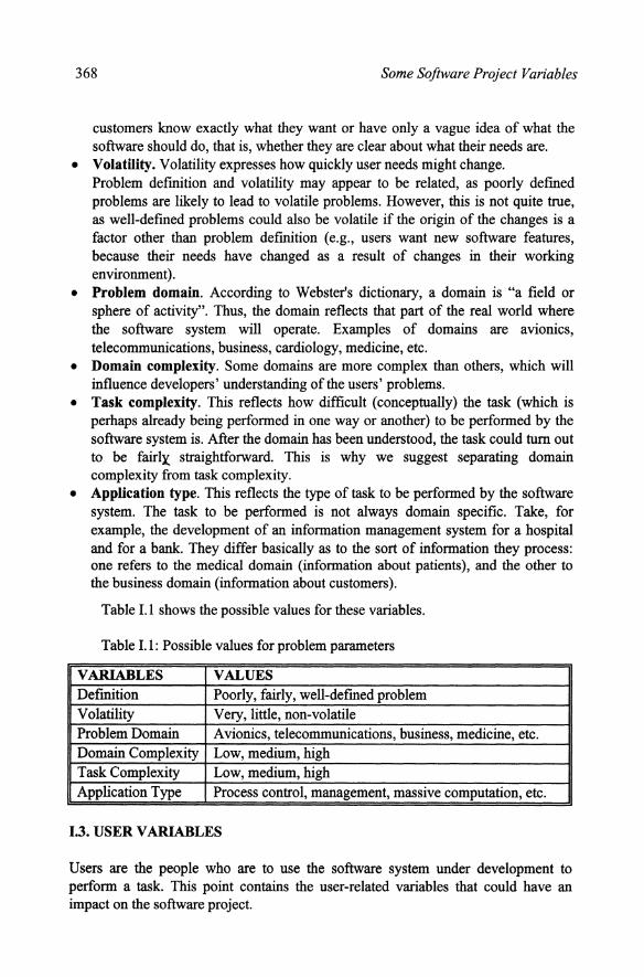
Table I. I shows the possible values for these variables.
Table I. I : Possible values for problem parameters
VARIABLES VALUES Definition Poorly, fairly, well-defmed problem Volatility Very, little, non-volatile Problem Domain Avionics, telecommunications, business, medicine, etc. Domain Complexity Low, medium, high Task Complexity Low, medium, high Application Type Process control, management, massive computation, etc.
1.3. USER VARIABLES
Users are the people who are to use the software system under development to perform a task. This point contains the user-related variables that could have an impact on the software project.

Basics of Software Engineering Experimentation 369
• Experience using computers. This refers to user experience in interacting with generic software applications, that is, commonly used applications, like word processors, operating systems, web, e-mail, etc.
• Experience using similar applications. This refers to user experience in interacting with software applications dealing with the same or similar tasks.
• Expertise in the task. This reflects how expert the user is at carrying out tasks like the one he/she will perform using the software.
Table 1.2 shows the possible values for these variables.
Table 1.2. Possible values for user variables
VARIABLES VALUES Experience using computer Novice, occasional, frequent user Experience using similar applications Novice, occasional, frequent user Expertise in the task Novice, qualified, expert
1.4. INFORMATION SOURCE VARIABLES
It will be necessary to gather the relevant information from the right sources in order to:
• understand the domain, • understand the task the software system is to perform, and • develop the system.
The characteristics of these sources of information could affect the software project as shown below:
• Type of sources. There are different sources from which the various types of information can be gathered. They range from experts in the domain and the task, literature, any similar software systems, future system users, etc.
• Availability. Availability of every information source. People may not always be available and some documents or software may have access restrictions.
• Co-operation. Willingness of the stakeholders to co-operate in software development. Irrespective of their availability, people may (or may not) be interested in co-operating on gathering information or during the software development process.
Table 1.3 shows the possible values for these variables.

370 Some Software Project Variables
Table 1.3. Possible values for infonnation sources variables
VARIABLES VALUES Type of sources Experts, literature, existing software, etc. Availability High, medium, low Co-operation High, medi~, low
1.4. DEVELOPER ORGANIZATION VARIABLES
The developer organisation will be the company, department or business unit (if the software is developed within the company) in charge of developing the software system.
Irrespective of the characteristics of the team of developers, the characteristics of the developer organisation in charge of developing the software system could also have an influence on the software project.
• Experience in problem domain. One relevant point will be whether the developer organisation as a whole has previous experience in developing software for the problem domain. The team of developers will always have somebody with experience whom they can consult if they have a problem.
• Experience in application type. Previous experience the company has in developing software that perfonns the sort of tasks in question. Again, the team of developers will always have somebody with experience whom they can consult.
• Experience with tools. Previous company experience in using the tools employed during the project. Introducing a tool that nobody in the developer organisation has ever used before is quite a different matter from introducing a tool that other people (not necessarily members of the team of developers) have used.
• Experience with methods. Previous company experience in using the methods being employed during the project. Again, introducing a method that nobody in the developer organisation has ever used before is quite a different matter from introducing a method that other people (not necessarily members of the team of developers) have used.
• Management attitude. How management feels about the tools and methods used in the project. If they are not confident about their usefulness, it will be hard (or sometimes impossible) to make them work.
• Personnel turnover. If there is a tendency for a high percentage of people to leave the company, new people are always joining, who might not be familiar with how things work at the company.
• Maturity level. Developer organisation projects are unlikely to have the same maturity level. However, the overall maturity level of the developer organisation will be significant.

Basics of Software Engineering Experimentation 371
Table 1.4 shows the possible values for these variables.
Table 1.4: Possible values for company variables
VARIABLES VALUES Experience in problem domain ~one, some, a lot Experience in application type ~one, some, a lot Experience with tools ~one, some, a lot Experience with methods ~one, some, a lot Management attitude Favourable, indifferent, unfavourable Personnel turnover High, medium, low Maturity level Initial, repeatable, defmed, managed,
optimising
1.5. CUSTOMER CONSTRAINTS
The stakeholders may impose some sort of restrictions on the fmal software system. These restrictions may vary depending on the task the software system has to perform. These include:
• Target platform. Characteristics of the target platform on which the software system is to operate. These characteristics include the description of both the hardware and the software that will interact with the software system.
• Response time constraints. Constraints the stakeholders may impose on the time it takes the software system to perform the task.
• Security constraints. Constraints the stakeholders may impose on how the software system handles the information.
• Safety constraints. Constraints the stakeholders may impose on how the software system responses could affect human beings.
• Testing constraints. Constraints the stakeholders may impose on how the testing procedure is performed when developing the system.
Table 1.5 shows the possible values for these variables.
Table 1.5: Possible values for software system variables
VARIABLES VALUES Target platform Description of hardware and software Response time constraints List of constraints Security constraints List of constraints Safety constraints List of constraints Testing constraints List of constraints
The stakeholders may also impose some sort of restrictions on the documentation

372 Some Software Project Variables
they are given along with the software system. These restrictions may vary depending on the users and the taSk the software system has to perform. They all have to be listed.
• Documentation constraints. Constraints the stakeholders may impose on the documentation they are given.
Table 1.6 shows the possible values for these parameters.
Table 1.6: Possible values for user documentation parameters.
VARIABLES VALUES Documentation constraints List of constraints
1.6. PROCESS VARIABLES
According to IEEE-Std-610, a process is a sequence of steps performed for a particular purpose. Therefore, the software process is the sequence of steps performed to develop a software system. Thus, this point contains the characteristics of the software development process that could have an impact on the software project.
• Maturity. The variables refer in this case to the maturity level of the project in question.
• Description. List of the phases and activities of which the software process will be composed, as well as their inputs and expected outputs.
• Relationships between activities. Defmition of interrelations between the phases, activities and products identified in the description.
• Life cycle. The life cycle is defined as the phases a software product goes through from when it is conceived to when it is no longer available for use. This variable reflects the type of life cycle to be followed in the project in question: waterfall, spiral, incremental, etc.
• Standards. Process and product standards to be respected during software development will have to be specified.
• Constraints. There could be constraints on the process that will affect the project, and they have to be taken into account. The constraints in a software project may vary from project to project, as they are heavily dependent on the situation. Some examples are: constraints on budget, delivery date, etc.
Table 1.7 shows the possible values for these variables.

Basics of Software Engineering Experimentation 373
Table I. 7: Possible values for process variables
VARIABLES VALUES Maturity Initial, repeatable, defmed, managed,
optimising Description ... Relationships between activities ... Life-cycle Waterfall, spiral, incremental, prototyping, etc. Constraints Budget, time, etc. Standards IEEE, PSS-5, etc.
Note that there is no parameter called risks. One might think that this is an important parameter. However, it has not been taken into account as risk encompasses (or should encompass) other parameters specified in this annex.
1.7. METHOD AND TOOL VARIABLES
A method is usually defmed as an organised approach based upon applying some technique. It has an associated technique, as well as a set of guidelines about how and when to apply the technique, when to stop applying it, when the technique is suited and how it can be evaluated.
This aspect contains variables related to methods and tools used in the development process that might have an impact on the software project.
• Methods used. Methods applied in each phase or activity of software development.
• Tools used. Tools used in each phase or activity of software development.
Table 1.8 shows the possible values for these variables.
Table 1.8: Possible values for the variables methods and tools
VARIABLES VALUES Methods Name of the methods used in each activity, etc. Tools Name of the tools used in each activity, etc.
1.8. TEAM VARIABLES
This aspect contains characteristics of the team of software developers working on the project that could have an impact on the software project.
• Size. Number of development group members. • Structuredness. Development teams are usually heterogeneous. This means that
they are composed of different sorts of people. This variable will reflect the
374 Some Software Project Variables
division of the development group by positions: Number and type of analysts, programmers, testers, quality, etc.
• Assignment. This will reflect the tasks or activities assigned to each team member.
• Level of communication. The level of communication of the group will differ depending on whether the team is located in the same building, same town, is a subcontractor, etc.
• Level of integration. This parameter will show the level of integration among the members of the group, which should ideally be high, but might not be.
• Level of excellence. Everybody is assumed to perform equally. However, irrespective of their experience, some people perform much better in practice.
• Background experience in domain. Experience of each member of the team in developing software systems in the domain in question or a similar field.
• Background experience in application type. Experience of each member of the team in developing software systems to solve the same or similar tasks.
• Knowledge of SE. Theoretical knowledge of software engineering of every member of the team.
• Experience in the software process. Each member's experience in the software process applied.
• Practical experience in SE. Each member's experience in software development.
• Experience of tools/methods. Each member's experience with the tools and methods used and similar ones.
• Experience in position. This reflects an individual's previous experience in performing project duties.
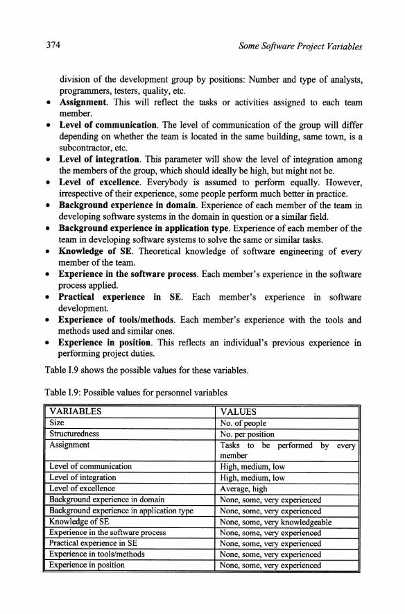
Table 1.9 shows the possible values for these variables.
Table 1.9: Possible values for personnel variables
VARIABLES VALUES Size No. of people Structuredness No. per position Assignment Tasks to be performed by every
member Level of communication High, medium, low Level of integration High, medium, low Level of excellence Average, high Background experience in domain None, some, very experienced Background experience in application type None, some, very experienced Knowledge of SE None, some, very knowledgeable Experience in the software process None, some, very experienced Practical experience in SE None, some, very experienced Experience in tools/methods None, some, very experienced Experience in position None, some, very experienced

Basics of Software Engineering Experimentation 375
1.10. PRODUCT VARIABLES
As mentioned in section 4.5.1, some characteristics of the intermediate products can affect other intermediate products, as products are developed on the basis of other products in software development. For example, variables that are used as response variables in experiments with a given intermediate product - correctness, validity or maintainability, for instance- can be said to also act as parameters in experiments involving other software products. By way of an example, requirements correctness could be a response variable for an experiment on the requirements phase and a variable influencing design in an experiment on the design phase. Therefore, suppose that we are comparing two design techniques in the latter example. In this case, specifications correctness must be fixed as a parameter if we do not intend to account for this. Thus, we will know that the conclusions of the experiment are valid concerning C correctness specifications. The other possibility is for specifications correctness to be considered in the experiment. The conclusions of such an experiment will tell us whether either of the design techniques is better, irrespective of specifications correctness (if the two factors do not interact), or which technique behaves better for each specifications correctness level (if the two factors interact).
However, these are not the only variables that will have an impact on the software project. There are others, like the architecture chosen or functionality of a module. Some of these variables are examined below. Readers are referred to section 4.4 Response Variables in SE Experiments for others. • Document legibility. The ease of reading and interpreting the information
described in the documents to be used as a basis for undertaking a given product is essential for the success of the implementation of the product in question. Thus, for example, it is essential for the documents generated during analysis to be easy for the designer to understand and the same can be said for the documents generated during design with respect to the programmer who is to use them to write the respective code.
• Size. The size of the product to be used as a basis for developing another product can have a major impact on the latter's development. Therefore, this variable should be taken into account.
• Software architecture. The software architecture describes the components of the system, their interactions, patterns used in its composition and the constraints and properties of these patterns. This would include the type of software and processing conditions.
• Module type. Modules can normally be grouped according to their main functionality for coding. For example, a software program can contain modules committed to calculation, control, input and output operations, error processing, etc.
Table 1.10 shows the possible values for these variables.

376 Some Software Project Variables
Table 1.10: Possible values for intermediate product variables
VARIABLES VALUES Document legibility None, little, a lot Size Large, medium, small Software architecture Pipes and filters, events and implicit invocation, object-
oriented organisation, multi-layer organisation, repositories, interpreters, process control.
Type of module Model calculations, user 1/0, control, error processing, help messages processing, moving data around, comments, data declaration.
Tables 1.11 and 1.12 summarise the variables explained above.
Table 4.11: External parameters for the software application domain
EXTERNAL PARAMETERS
PROBLEM STAKEHOLDERS COMPANY CUSTOMER CONSTRAINTS
USER INF SOURCES
Definition Experience using Type Experience in Target platform Volatility (stability) computers Availability problem domain Response time Problem domain Experience using Co-operation Experience in constraint Domain complexity similar apps. application type Security constraint Task complexity Expertise in the Experience with Safety constraint Application type task tools Testing constraint
Experience with Documentation methods constraints Management attitude Personnel turnover Maturity level

Basics of Software Engineering Experimentation 377
Table 4.12: Internal parameters for the software application domain
INTERNAL PARAMETERS PROCESS METHODS &TOOLS TEAM PRODUCTS Maturity Methods used Size Document legibility Description Tools used Structuredness Size Relationships Assignment Software architecture between activities Level of communication Module type Life cycle Level of integration Constraints Excellence Standards Experience in domain
Experience in appl. type Knowledge of SE Experience in sw process Practical experience in SE Tools/methods experience Experience in position

ANNEX II: SOME USEFUL LATIN SQUARES AND HOW THEY ARE USED TO BUILD
GRECO-LATIN AND HYPER-GRECO-LATIN
SQUARES
11.1. A BIT OF HISTORY
During the later years of his life, Euler wrote a voluminous report about some magic squares that are now referred to as Latin squares, because Euler chose to label their cells using Latin letters rather than using the customary Greek alphabet.
Consider the square shown in Figure II.l.(a), for example. The four Latin letters a, b, c and d are arranged in the sixteen cells of the square so that each letter appears once and only once in each row and each column. Figure ll.l(b) shows a different square, whose cells are marked with Greek letters. If these two squares are superposed, as shown in Figure II.l(c), each Latin letter is found to be associated once and only once with each Greek letter. When two or more squares can be combined in this manner, the squares are said to be orthogonal. The resulting square is then referred to as a Greco-Latin square.
a b c d a ~ e 8 aa b~ ce d8
b a d c e 8 a ~ be a8 da c~
c d a b 8 e ~ a c8 de a~ ba
d c b a ~ a 8 e d~ ca b8 ae
(a) (b) (c)
Figure 11.1. Greco-Latin squares
Anecdotally, the right-hand square can be said to solve a game of patience that was very popular during the l81h century. The aces, kings, queens and jacks of all the suits are removed from an ordinary pack of cards. The aim is to arrange them in a square so that each row and column contains the four values and the four suits.
Even in Euler's time, it was not hard to prove that there were no Greco-Latin squares of order 2. Squares of order 3, 4 and 5 were known, while a question mark hung over squares of order 6. Euler set out the problem as follows: there are six regiments on the square, each one of which has six officers, one for each of the six ranks. Can these thirty-six officers be arranged in a square formation so that each row and column contains one officer of each rank and from each regiment? Euler himself proved that the problem of the n2 officers, identical to building a GrecoLatin square of order n, could be solved provided that n was odd or "a pair of even class", that is, a multiple of four. After making several unfruitful attempts, Euler fmally stated that he had no doubt that it was impossible to fmd a complete square

380 Latin, Greco-Latin and Hyper-Greco-Latin Squares
of thirty-six cells and this also applied to n=lO, n=l4 and, generally, all orders "pairs of odd class"; that is, "pairs not divisible by four". This is Euler's famous conjecture. It can be stated more formally as follows: there is no pair of orthogonal Latin squares of order n=4k + 2, where k is any positive integer.
Tarry published a proof confmning the validity of Euler's conjecture for the order 6 in 1901.
However, Parker, from Univac, and Bose and Shrikhande, from the University of North Carolina, shattered Euler's hypothesis by discovering methods for building Greco-Latin squares of order 10, 14, 18 and 22. Pursuant to Euler's hypothesis, specialists had considered these squares out of the question for 167 years.
Sir Ronald Fisher was the first to show how the magic squares could be used in agronomic research. Consider, for example, the effects of seven chemical products on wheat growth. One of the difficulties with this sort of trials was that the fertility of the different parts of the same piece of land generally varies very unevenly. To be able to simultaneously test the seven chemical products and eliminate the bias due to the difference in land fertility, the experiment has to be planned as follows: divide the wheat field into plots that are the cells of a seven by seven square and apply the seven treatments according to a randomly selected Latin square. Taking into account this structure, a simple statistical analysis will account for the biases due to variations in land fertility.
Suppose that we now have the same experiment with seven varieties of wheat instead of just one. This fourth variable, the other three are fertility in the rows, fertility in the columns and treatment type, can be accounted for by now using a Greco-Latin square. The Greek letters specify where the different chemical products should be applied. The statistical analysis of the results is still simple.
The use of Greco-Latin squares is very well documented in experimental design in biology, medicine, etc. The plot obviously does not necessarily have to be a piece of land. It can be a cow, a patient, a form, a cage of guinea pigs, the site of an injection, a period of time or even an observer or group of observers. The GrecoLatin square is no more than a diagram of the experiment. Its rows are used to represent one variable, its columns, another and the Latin and Greek symbols, the third and fourth variables, respectively. For example, a medical researcher may want to test the effects of five different sorts of tablets, one of which is placebo, on people of five age groups, classed by five weight intervals and suffering from a complaint whose severity is rated on a scale of I to 5. The most efficient research method will be a Greco-Latin square of order 5, selected at random from the different possibilities of this order. Other variables can be taken into account by superposing more Latin squares. However, it is important to bear in mind that there will never be any more than n-1 mutually orthogonal squares for a given order n.
The history of the research that was to lead Parker, Bose and Shrikhande to discover the Greco-Latin squares of orders 10, 14, 18 and 22 dates back to 1958 with Parker's discovery that cast serious doubt on the accuracy of Euler's hypothesis. Following Parker's guidelines, Bose established some sound general rules for building Greco-Latin squares of large orders. Bose and Shrikhande then applied

Basics of Software Engineering Experimentation 381
these rules and were able to build a Greco-Latin square of order 22. This disproved Euler's conjecture, as 22 is an even number not divisible by four.
Some useful Latin and Greco-Latin squares are shown below.
11.2. 3X3 LATIN AND GRECO-LATIN SQUARES
Some 3x3 Latin squares are shown below. Remember that before executing a Latin square or similar design, we have to make sure that the design has been randomised. This can be done by randomly permuting first the rows and then the columns and fmally randomly assigning the alternatives to the letters.
3 X 3 ABc BCA CAB
ABC CAB BCA
The two designs are superposed to form a 3x3 Greco-Latin square. Using Greek letters for the second 3x3 Latin square, we get:
Aa.. Bl3 Cy By Ca. Al3 Cl3 Ay Ba..
11.3. 4X4 LATIN AND GRECO-LATIN SQUARES
Let's take a look at some 4x4 Latin squares.
4x4 ABCD BADC CDAB DCBA
ABCD DCBA BADC CDAB
ABCD CDAB DCBA BADC
These three 4x4 Latin squares can be superposed to form a Hyper-Greco-Latin square. The superposition of any two yields a Greco-Latin square.
11.4. SXS LATIN AND GRECO-LATIN SQUARES
Some 5x5 Latin squares are shown below.
5x5 ABC DE BCDEA CDEAB DE ABC EABCD
ABC DE CDEAB EABCD BCDEA DE ABC
ABC DE DEABC BCDEA EABCD CDEAB
ABC DE EABCD DE ABC CDEAB BCDEA
These 5x5 Latin squares can be superposed to form a Hyper-Greco-Latin square. Again, the superposition of any three yields a Hyper-Greco-Latin square design. Similarly, the superposition of any two yields a Greco-Latin square.

382 Latin, Greco-Latin and Hyper-Greco-Latin Squares
11.5. 6x6 LATIN SQUARES
Let's examine a 6x6 Latin square.
6x6 ABCDEF BAFECD CFBADE DCEBFA EDAFBC FEDCAB
6x6 Greco-Latin squares do not exist.
11.6. 7x7 LATIN AND GRECO-LATIN SQUARES
Two possible 7x7 Latin squares are as follows.
7x7 ABCDEFG BCDEFGA CDEFGAB DEFGABC EFGABCD FGABCDE GABCDEF
ABCDEFG CDEFGAB EFGABCD GABCDEF BCDEFGA DEFGABC FGABCDE
These two 7x7 Latin squares can be superposed to yield a Greco-Latin design.
11.7. 8X8 LATIN AND GRECO-LATIN SQUARES
Let's look at two possible 8x8 Latin squares.
8x8 ABCDEFGH BADCFEHG CDABGHEF DCBAHGFE EFGHABCD FEHGBADC GHEFCDAB HGFEDCBA
ABCDEFGH EFGHABCD BADCFEHG FEHGBADC GHEFCDAB CDABGHEF HGFEDCBA DCBAHGFE
These two 8x8 Latin squares can be superposed to yield a Greco-Latin design.
See (Box, 1978), for example, for other Latin square designs.

Basics of Software Egineering Experimentation 383
ANNEX Ill: STATISTICAL TABLES
Table III.l. Normal Distribution
z 0.00 0.01 0.02 O.o.J 0.04 0.05 0.06 0.07 O..OH 0.09
o.o 0.5000 0.4960 0.4920 0.41180 0.41140 0.4801 0.47111 0.4721 0.46111 0.4641 0.1 0.4602 0.4562 0.4522 0.44R.l 0.4443 0.4404 0.4364 0.4325 0.42116 0.4247 0.2 0.4201 0.4168 0.4129 0.4090 0.40~2 0.4013 0 .. \974 O .. W.\6 0.]1197 0.3!1~9 0.3 0.1821 0.178.\ 0.3745 03707 0 .. 11\1\9 0._11\32 0 .. 1594 ll..l557 O.JS2U O .. l4K.1 0.4 0.1446 0.3409 0.3.\72 0.33.\6 ll..l.l<lO 0.3264 O .. l12K 0 .. 11'12 0.3156 03L!I 0.5 0..10115 0.30~ 0.3015 0.29111 0.2"41\ 0.2912 0.21177 11.:!1143 tt2KIO 0.2776 0.6 !L!74J 0.2709 0.2676 0.264.1 0.2611 0.2578 0.2546 11.2514 11.2411] 0.2451 0.7 0.2420 0.23119 0.2.\58 0.2327 0.2296 0.2266 0.2236 0.22116 11.2177 0.21411 0.11 0.2119 0.2090 0.2061 0.20H 0.2005 0.1977 0.1949 0.11122 0.1894 O.IH67 0.9 0.11141 0.11114 0.17R8 0.1762 0.1736 0.1711 0.11\115 0.1660 0.11\.\5 0.11\11 1.0 0.1587 0.1~62 0.15.\9 0.151~ 0.14112 0.1469 0.1446 0.1423 0.1401 0.1.'711 1.1 O.IJ~7 O.IJ.lS 0.014 0.1292 0.1271 0.1251 0.1230 0.1210 0.1190 0.1170 1.2 0.1151 O.IIJI 0.1112 0.1091 0.1075 0.1056 0.10]11 11.1010 0.100.1 O.tl9K5 1.3 00968 O.!H51 0.0934 0.0918 0.0901 O.OK85 IHIII69 1Hlii5J llOKlX 0.08n 1.4 0.0808 0.079.\ 0.0778 0.071\4 00749 11.07.15 0.0721 0.070K ll0694 0.0681 1.5 0.0668 0.06.55 0.064.1 0.0630 0.061 K 0.0606 0.0594 0.05112 IJ.0571 0.055'1 1.6 0.0548 0.05]7 0.0526 0.0516 00505 0.()4<15 0.04115 0.0475 0.0465 0.045~
1.7 0.0446 0.04.16 0.0427 0.04111 0.(l409 0.0401 0.0392 O.OJM4 0.0375 0.0.167 1.8 0.0359 0.0.\51 0.0344 O.OJ.\6 0.0.129 0.0.122 0.0314 0.0.107 0.0301 0.0294 1.9 0.0287 0.0281 0.0274 0.0268 0.0262 0.0256 0.02~ 0.0244 0.0239 0.02.\.l 2.0 0.02211 0.0222 0.0217 0.0212 0.0207 0.0202 0.0197 0.01112 0.01811 0.01113 2.1 0.0179 0.0174 0.0170 0.0166 0.0162 O.OIS~ 0.0154 O.QI~ 0.0141\ 0.0143 2.2 0.0139 0.0136 0.0132 0.0129 0.0125 0.0122 0.0119 0.0116 0.011.1 0.0110 2 . .\ 0.0107 0.0104 0.0102 0.009'1 0.1)()1)6 0.0094 OJ)(l91 Otxlll\1 O.llOA7 0.00114 2.4 O.IKlllc 0.!)(180 0.0071C 0_()(175 0.1)(17.\ 0.1!071 0Jl06'1 01!068 0(1066 0.0064 2.~ 0.0062 11.0060 0.0059 0.11057 0.()(155 0.0054 0.1!052 0.0051 11.0049 0.0048 2.6 0.()(147 0.0045 0.0044 0.004.\ 0.0041 0.0040 Q.OOJ9 0.00311 0.0037 0.0036 2.7 0.00.\5 0.0034 O.OOH 0.0032 0.0031 0.0030 0.0029 0.0028 0.0027 0.0026 2.8 0.0026 O.ll025 0.0024 0.0023 O.txi2J 0.0022 0.0021 OIXI21 0.0020 0.0019 2. 9 0.11019 0.00 Ill 0.00 ll! O.llO 17 0.01116 0.()(116 O.()(ll 5 O.!Kl I 5 0.0014 0.()(114 3.0 0.0013 0.001.\ 0.0013 110012 001112 0.0011 0.0011 0.0011 0.0010 0.0010 3.1 0.0010 0.0009 0.0009 0.0009 0.0008 0.0008 0.0008 0.0008 0.0007 0.0007 3.2 0.0007 0.0007 0.0006 0.0006 0.0006 0.0006 0.0006 0.0005 0.0005 0.0005 3.3 0.0005 0.0005 0.0005 0.0004 0.0004 0.0004 0.0004 O.txl04 O.IXXl4 0.000.\ .\.4 0.000.\ 0.0003 0.0003 0.000.1 0.0003 0.000] 0.0003 0.000.\ 0.0003 0.0002 -'-~ 0.0002 0.0002 0.()()02 0.00:12 0.0002 0.0002 0.0002 0.0002 0.0002 0.0002 .\.6 0.0002 0.0002 0.0001 0.0001 0.0001 0.0001 0.0001 0.0001 0.0001 0.0001 ,\.7 0.0001 0.0001 0.0001 0.0001 0.0001 0.0001 0.0001 0.0001 0.0001 0.0001 .l.K 0.0001 0.0001 0.0001 0.0001 0.0001 0.0001 0.0001 0.0001 0.0001 0.0001 .\.9 0.0000 0.0000 0.0000 0.0000 0.0000 0.0000 0.0000 0.0000 0.0000 0.0000

384 Annex III: Statistical Tables
Table III.2. Nonnal Probability Paper.
N " 18 N • 32 N • &l N "' 15 N • 31 N • 83
"

Basics of Software Egineering Experimentation 385
Table III.3. Student's t Distribution.
Probability of the tail area
" 8.4 1.35 ... U5 0.025 •••• 0.805 U825 UIJI 8.0085
I o.m 1.000 3.078 6.314 12.706 31.821 63.657 127.32 318.31 636.62 2 0.289 0.816 1.886 2.920 4.303 6.965 9.925 14.089 22.326 31.591 3 0.277 0.765 1.638 2.353 3.182 4.541 5.841 7.453 10.213 12.924 .. 0.271 0.741 1.533 2.132 2.776 3.747 4.604 5.598 7.173 8.610 5 0.267 0.727 1.476 2.015 2.571 3.365 4.032 4.773 5.893 6.869 6 O.Z65 0.718 1.440 1.943 2.447 3.143 3.707 4.317 5.201 5.959 7 0.263 0.711 1.415 1.895 2.365 2.998 3.499 4.029 4.785 5.408
• 0.262 0.706 1.397 1.860 2.306 2.896 3.355 3.833 4.SOI 5.041 9 0.261 0.703 1.383 1.833 2.262 2.821 3.2j() 3.690 4.297 4.781
10 0.260 0.700 1.372 1.812 2.228 2.764 3.169 3.581 4.144 4.587 II 0.260 0.697 1.363 1.796 2:201 2.718 3.106 3.497 4.025 4.437 IJ 0.259 0.695 1.3St 1.782 2.179 2.681 3.055 3.428 3.930 4.318 13 0.259 0.694 J.JSO 1.771 2.160 2.6SO 3.012 3.372 3.852 4.221 14 0.2S8 0.692 1.345 1.761 2.145 2.624 2.977 3.326 3.787 4.140 15 0.258 0.691 1.341 1.753 2.131 2.602 2.947 3.286 3.733 4.073 16 0.258 0.690 1.337 1.746 2.120 2.583 2.921 3.252 3.686 4.015 17 0.257 0.689 1.333 1.740 2.110 2.567 2.898 3.222 3.646 3.965 II 0.257 0.688 1.330 1.734 2.101 2.552 2.878 3.197 3.610 3.922 19 0.257 0.688 1.328 1.729 2.093 2.539 2.861 3.174 3.579 3.883 10 0.257 0.687 1.325 1.725 2.086 2.528 2.845 3.153 3.552 J.Sj() 11 0.257 0.686 1.323 1.721 2.080 2.518 2.831 3.135 3.527 3.819 11 0.256 0.686 I.J21 1.717 2.074 2.S08 2.819 3.119 3.S05 3.792 23 0.256 0.685 J.JI9 1.714 2.069 2.500 2.807 3.104 3.485 3.767 14 0.256 0.685 1.318 1.71 I 2.064 2.492 2.797 3.091 3.467 3.745 Z5 0.256 0.684 1.316 1.708 2.060 2.48S 2.787 3.078 3.4SO 3.725 26 0.256 0.684 I..'JIS 1.706 2.056 2.479 2.779 3.067 3.435 3.707 27 0.2.56 0.684 1.314 1.703 2.052 2.473 2.771 3.057 3.421 3.690 21 0.256 0.683 1.313 1.701 2.048 2.467 2.763 3.047 3.408 3.674 19 0.256 0.683 I.JII 1.699 2.045 2.462 2.756 3.038 3.396 3.659 30 0.2.56 0.683 1.310 1.697 2.042 2.457 2,7j() 3.030 3.385 3.646 40 0.255 0.681 1.303 1.684 2.021 2.423 2.704 2.971 3.307 3.SSI 60 0.2,. 0.679 1.296 1.671 2.000 2.390 2.660 2.915 3.232 3.460
120 0.254 0.677 1.289 1.658 1.980 2.358 2.617 2.860 3.160 1373 ao 0.253 0.674 1.282 1.645 1.960 2.326 2.576 2.807 3.090 3.291
386 Annex III: Statistical Tables
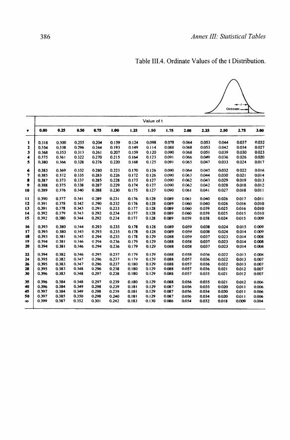
Table III.4. Ordinate Values of the t Distribution.
~ e
Value oft
" 0.00 0.25 0.50 8.75 1.00 1.25 1.50 1.75 1.00 1.25 1.50 1.75 3.00
I 0.318 0.300 0.255 0.204 0.159 0.124 0.098 0.078 0.064 0.053 0.044 0.037 0.032 1 0.354 0.338 0.296 0.244 0.193 0.149 0.114 0.088 0.068 0.053 0.042 0.034 0.027 3 0.368 0.353 0.313 0.261 0.207 0.159 0.120 0.090 0.068 0.051 0.039 0.030 0.023 4 0.375 0.361 0.322 0.270 0.215 0.164 0.123 0.091 0.066 0.049 0.036 0.026 0.020 5 0.380 0.366 0.328 0.276 0.220 0.168 0.125 0.091 0.065 0.047 0.033 0.024 0.017
6 0.383 0.369 0.332 0.280 0.223 0.170 0.126 0.090 0.064 0.045 0.032 0.022 0.016 7 0.385 0.372 0.335 0.283 0.226 0.172 0.126 0.090 0.063 0.044 0.030 0.021 0.014 I 0.387 0.373 0.337 0.285 0.228 0.173' 0.127 0.090 0.062 0.043 0.029 0.019 0.013 9 0.388 0.375 0.338 0.287 0.229 0.174 0.127 0.090 0.062 0.042 0.028 0.018 0.012
10 0.389 0.376 0.340 0.288 0.230 0.175 0.127 0.090 0.061 0.041 0.027 0.018 0.011
II 0.390 0.377 0.341 0.289 0.231 0.176 0.128 0.089 0.061 0.040 0.026 0.017 0.011 I:Z 0.391 0.378 0.342 0.290 0.232 0.176 0.128 0.089 0.060 0.040 0.026 0.016 0.010 13 0.391 0.378 0.343 0.291 0.233 0.177 0.128 0.089 0.060 0.039 0.025 0.016 0.010 14 0.392 0.379 0.343 0.292 0.234 0.177 0.128 0.089 0.060 0.039 0.025 O.QIS 0.010 IS 0.392 0.380 0.344 0.292 0.234 0.177 0.128 0.089 0.059 0.038 0.024 O.DI5 0.009
16 0.393 0.3110 0.344 0.293 0.235 0.178 0.128 0.089 0.059 0.038 0.024 0.015 0.009 17 0.393 0.380 0.345 0.293 0.235 0.178 0.128 0.089 0.05'.1 0.038 0.024 0.014 0.009 II 0.393 0.381 0.345 0.294 0.235 0.178 0.129 0.088 0.05'.1 0.037 0.023 0.014 0.008 19 0.394 0.381 0 .. 146 0.294 0.236 0.179 0.129 0.088 0.058 0.037 0.023 0.014 0.008 :zo 0.394 0.381 0.346 0.294 0.236 0.179 0.129 0.088 0.058 0.037 0.023 0.014 0.008
:n 0.394 0.382 0.346 0.295 0.237 0.179 0.129 0.088 0.058 0.036 0.022 0.013 0.008 24 0.395 0.382 0.347 0.296 0.237 0.179 0.129 0.088 0.057 0.036 0.022 0.013 0.007 Z6 0.395 0.383 0.347 0.296 0.237 0.180 0.129 0.088 0.057 0.036 0.022 0.013 0.007 Z8 0.395 0.383 0.348 0.296 0.238 0.180 0.129 0.088 O.OS7 0.036 0.021 0.012 0.007 30 0.396 0.383 0.348 0.297 0.238 0.180 0.129 0.088 0.057 O.D35 0.021 0.012 0.007
35 0.396 0.384 0.348 0.297 0.239 0.180 0.129 0.088 0.056 0.035 0.021 0.012 0.006 40 0.396 0.384 0.349 0.298 0.239 0.181 0.129 0.087 0.056 0.035 0.020 0.011 0.006 45 0.397 0.384 0.349 0.298 0.239 0.181 0.129 0.087 0.056 0.034 0.020 0.011 0.006 50 0.397 0.385 0.350 0.298 0.240 0.181 0.129 0.087 0.056 0.034 0.020 0.011 0.006 ... 0.399 0.387 0.352 0.301 0.242 0.183 0.130 0.086 0.054 0.032 0.018 0.009 0.004

Basics of Software Egineering Experimentation 387
Table III.5. 90-Percentiles of the F(v 1, v2) Distribution.
~ I I 3 ' 5 6 7 I ' .. ll 15 lO 14 3t 40 60 110 Ill
' I 39.16 49.l0 13.S9 IS.I3 S7J4 18.20 11.91 19.44 S9.!6 60.19 60.71 61.22 61.74 62.00 6~.26 61.13 62.79 63.06 63.33 2 &.Sl 9.00 9.16 9.14 929 9.)3 9.)1 9.)1 9.)8 9.)9 9.41 9.41 9.44 9.41 U6 9.41 9.41 9.48 9.4'1 J 1.14 1.46 S.l9 S.l4 1.31 1.21 1.21 S.2S 1.24 S.ll S.22 S.20 1.18 I. II 1.11 1.16 1.11 1.14 1.13 4 4.14 4.32 4.19 4.11 4.0S 4.01 191 3.91 3.94 3.92 3.'10 3.17 3.84 JJ3 3.12 ).10 3.79 3.11 3.76 5 4.06 3.71 162 3.12 141 l . .O l.J7 134 3.32 l.lO 127 124 121 119 3.17 116 3.14 3.12 l.IO 6 m 3.46 3.29 l.IB l.11 3.01 l.OI 2.98 2.96 2.94 l.'IO 2.87 2.84 2.82 2.80 2.78 2.16 2.14 2.72 7 l.S9 3.26 3.07 2.96 l.BI 2.83 2.11 l1j 2.72 2.10 l61 2.63 2.19 !.18 2.56 2.14 2.11 2.49 w I 3.46 3.11 292 2.81 2.73 2.67 2.61 259 2.l6 1.14 I.SO 2.46 2.42 2.40 lJ8 2.36 ll4 2J2 l29
' ).36 3.01 2.81 2.69 2.61 lll 2.51 l47 2.44 1.42 I.J8 2.34 2.30 2.28 l.ll 2.23 2.21 2.18 2.16 10 129 2.92 2.7) 2.61 2.12 2.46 2.41 138 1.31 132 1.28 2.14 2.20 liB 2.16 2.1l w 2.01 1.06 II 3.23 2.16 2.66 2.14 2.41 2.39 2.34 2.30 2.21 2.21 2.21 2.11 2.12 2.10 2.(1 2.05 2.03 2.00 1.97 IZ 3.11 2.11 2.61 2.48 2.39 2.33 2.21 2.24 2.21 2.19 2.11 2.10 2.06 2.04 2.01 1.99 1.96 1.93 1.90 ll 3.14 2.16 2.16 2.4) 2.31 2.28 2.2) 2.20 2.16 2.14 2.10 l.OS 2.01 1.98 1.96 1.93 1.!10 1.88 us 14 l.IO 2.7) 2.12 2.39 2.31 2.24 2.19 2.11 2.12 2.10 2.01 2.01 1.96 1.94 1.91 1.89 1.16 1.13 1.80 15 lD7 2.10 2.49 2.36 2.21 l.l1 116 2.1! lO'I 2.06 2.02 1.97 1.92 1.'10 1.17 1.11 1.82 1.19 1.76 16 3.01 2.67 !.46 2.3) 2.24 2.18 2.13 2.~ 2.06 !OJ 1.!19 1.94 1.11' 1.81 1.14 1.81 1.71. 1.71 1.72 11 3.03 2.64 2.44 2.31 2.22 I. II 2.10 2.06 2.03 2.00 1.96 1.91 1.16 1.14 1.81 1.71 1.71 1.12 1.69 II lDI 1.6l 2.42 2.29 2.20 2.13 !.01 1.04 ~.00 1.98 1.93 1.89 1.84 1.81 1.'11 1.'15 1.12 1.69 1.66 19 2.99 2.61 2.40 2.27 liS 2.11 l.CJ6 1.02 1.98 1.96 1.91 1.16 1.11 1.79 1.16 1.73 1.'10 1.67 1.63 lO 2.97 2.19 1.38 2.25 !.16 2.09 2,04 2.00 1.96 1.94 1.89 1.84 1.19 1.77 1.14 1.71 1.68 1.64 1.61 11 2.96 2.11 2.36 2.23 2.14 2.08 2.02 1.98 1.95 1.91 1.11 1.83 1.18 1.11 1.12 1.69 1.66 1.62 1.59 :u 2.91 2.l6 2.35 l2l l.ll 2.06 2.01 1.97 1.93 1.'10 1.16 1.81 1.76 1.13 1.70 1.61 1.64 1.60 1.57 2J 2.94 l.ll 2.34 2.21 2.11 2.01 1.99 1.91 1.92 1.11' 1.84 1.80 1.74 1.72 1.69 1.66 1.62 1.19 I.SS 24 2.93 2.54 l.)J 2.19 2.10 1.04 1.91 1.94 1.91 1.11 1.83 1.11 1.73 1.10 1.61 1.64 1.61 1.!7 1.13 IS 2.92 2.53 2J2 2.11 2.09 2.02 1.91 1.93 1.89 1.87 1.82 1.11 1.72 1.69 1.66 1.63 1.19 i.l6 l.l2 26 2.91 2.52 2.31 2.11 1.08 2.01 1.96 1.91 1.81 1.16 1.11 1.76 1.71 1.61 1.61 1.61 1.58 1.14 I.SO 27 2.'10 2.51 l.JO 111 2.01 2.00 1.95 1.91 1.&1 Ill 1.10 1.7l 1.'10 1.67 1.64 1.60 1.51 1.!3 1.49 II 2.89 llO 1.29 2.16 2.06 2.00 1.94 1.90 1.81 1.84 1.19 1.74 1.6'1 1.66 1.6) 1.59 l.l6 1.52 1.48 29 1.89 2.10 1.28 lll 2.06 I.W 1.93 1.89 1.86 1.1~ 1.18 1.7) 1.68 1.61 1.62 1.58 l.ll l.lll 1.41 JO 2.81 2.49 2.28 2.14 2.05 1.91 1.93 1.88 1.85 1.12 1.77 1.12 1.61 1.64 1.61 1.11 1.14 1.10 i 1.46 40 2.84 2.44 2.23 2.0'1 2.00 1.93 1.11 1.8) 1.79 1.16 1.71 1.66 1.61 l.l7 1.54 l.ll 1.47 1.42 IJ8 60 2.1'1 2.39 2.18 2.04 1.91 1.17 1.12 1.77 1.14 1.71 1.66 1.60 1.14 1.51 1.48 1.44 1.40 IJl 1.29
110 2.15 2.35 lll 1.99 1.!10 1.82 1.71 1.72 1.68 1.61 1.60 l.ll 1.48 1.4l 1.41 1.37 1.32 1.26 1.19 Ill 171 2.l0 2.01 194 l.ll 1.11 1.72 1.61 1.63 1.60 l.ll 1.49 1.42 I.JI 1.34 1.30 1.24 1.17 1.00

388 Annex III: Statistical Tables
Table III.6. 95-Percentiles of the F(v~o v2) Distribution.
I~ I z J 4 5 ' 7 I ' It 12 15 • :w Jt • " 121 ao
' I 161.4 IIJ9 • .l 215.7 ~.6 2l0.2 m.o 2J6J 2.lU 2.,5 241.9 243.9 245.9 241.0 249.1 250.1 251.1 252.2 2SJ.3 254.3 2 11.51 19.00 19.16 19.25 19 . .!0 19.33 19.J5 19.l7 19.31 19AO 19.41 19.43 19.4! IUS 19.<16 19.47 19.41 19.49 19.50 3 10.13 9.55 9.21 9.12 9.01 1.94 1.19 us 1.11 1.7'1 1.74 1.70 1.66 1.64 1.62 1.59 1.57 us 1.!3 4 7.71 6.94 6.59 6.39 6.26 6.16 6.15 6.04 6.00 5.96 5.91 5.16 S.IO S.71 !.7! s.n S.69 5.66 S.63 5 6.61 5.79 SAl 5.19 5.05 4.9S 4.11 4.12 4.77 4.74 4.68 4.62 4.56 4.S3 4.50 4.46 4.43 uo 4.36
• 5.99 S.l4 4.76 4.S3 4 . .19 4.28 4.21 4.15 4.10 4.06 4.00 3.94 3.87 3.14 3.11 3.71 174 3.70 3.67 7 5.59 4.74 4.35 4.12 3.97 )J7 3.7'1 3.7} 3.61 3.64 J.S7 HI 144 !.41 3.31 3.34 1.!0 3.27 3.23 I 5.32 4.<16 4.07 114 3.69 1511 3JO 3.44 3.39 3.35 3.21 3.22 3.15 3.12 3.01 3.04 3.01 2.97 2.93 • 5.1~ 4.26 3.16 3.63 3.48 3.37 3.29 l.lJ 3.11 3.14 3.07 101 2.94 2.90 2.16 2.83 2.79 2.7S 2.71
10 4.96 4.10 3.71 141 3.33 3.22 3.14 3.07 3.02 2.98 2.91 liS 2.77 2.74 2.70 2.66 2.62 2.511 2.54 II 4.14 ].911 3.59 3.36 3.20 3.09 3.01 2.95 2.90 2.15 2.79 2.72 2.6.5 2.61 2.57 2 . .53 2.49 2.45 2.40 12 4.75 ).19 3.49 3.26 3.11 3.00 2.91 2.15 2.10 2.7! 2.69 2.62 2.54 2.51 2A7 2.43 2.31 2.34 2.30 ll 4.67 3.11 3.41 111 3.03 2.92 2J3 2.77 2.71 2.67 2.60 2.!3 2.<16 2.42 2.31 2.34 2.30 2.25 2.21 14 4.60 l74 ).34 111 2.96 2.15 2.76 2.70 2.65 2.60 2.53 2.46 2.)9 2.35 2.31 2.27 %.22 2.18 113 15 4.54 l611 3.29 3.06 2.90 2.79 2.71 2.64 2..59 2.54 2.<16 2.40 2.33 2.29 2.25 2.20 ).16 2.11 2.07 16 4,4\1 3.6J ).24 3.01 2.15 lT4 2.66 159 2.54 2.49 2.42 us 121 2.24 2.19 2.15 2.11 2.06 2.01 17 4.45 159 llO 2.96 2.81 2.70 2.61 2.55 2.49 2.45 2.38 2.31 2.ll 2.19 2.15 2.10 2.06 2.01 1.96 II 4.41 3.55 3.16 2.93 2.77 ~.66 2.SB 2.51 2.46 2.41 2.34 2.27 2.19 2.1S 2.11 2.06 2.02 1.97 1.92 .. 4,)! 3.52 3.1.1 2.90 2.14 2.63 2.54 2.4~ 2.42 2.31 2.31 2.23 2.16 2.11 2.07 2.03 1.98 1.93 1.11 10 4..15 3.49 110 2.87 2.71 2.60 Ul 2.45 2.39 2.15 2.21 120 2.12 l.CJI 2.04 1.99 1.95 1.90 1.14 21 4.J2 3.47 ].07 2.14 2.6M 2.57 2.49 142 Z.37 Z.l2 ll$ 2.11 2.10 2.05 2.01 1.96 1.92 U7 IJI 22 4.)0 ).44 lOS lJ2 2.66 2.5S 2.<16 2.40 U4 2.30 l.ll 2.1! 2.07 2.03 1.91 1.94 1.19 1.14 1.78 Z3 4.:!1! '-42 10) 2.10 2.64 2..53 2.44 2.37 U2 2.27 2.20 lll 2.0! 2.01 1.96 1.91 IJ6 1.11 1.16 u
··~ ).40 l.Ol 2.111 2.62 l.Sl 2.42 2J6 l.JO 2.25 2.11 lll 2.03 1.91 1.94 1.19 IJ4 1.79 1.1l
25 U4 ).)9 2.9'1 2.76 2.60 2.49 2.40 2.34 2.211 2.24 2.16 2.09 2.01 1.96 1.92 1.17 1.12 1.77 1.71 2t 4 . .!) ).37 l.'lll 2.74 2.59 2.47 2.39 2J2 2.27 2.22 liS 2.07 1.99 1.95 1.90 1.15 1.80 1.1S 1.69 l7 4.21 ),15 1.96 2.7) l.Sl 2.46 2.37 2.31 l.lS 2.20 2.1) 2.06 1.97 1.9) 1.18 1.14 1.79 1.73 1.67 Jl 4.211 3.34 2.9S 2.71 2.56 2.45 2.36 2.29 2.24 2.19 2.12 2.04 1.96 1.91 1.17 1.82 1.71 1.71 1.65 19 4.11 ).)) l.9J 2.711 HS 2.4J lJS 2.21 2.22 2.18 2.10 2.03 1.94 1.90 IJS 1.11 1.75 1.70 1.64 lG 4.17 l.ll m 2.69 2.53 l.42 2.33 2.27 2.21 2.16 2.09 2.01 1.9) 1.19 1.84 1.79 1.74 1.61 1.62 40 4.CJI 3.2.1 2.U 2.61 l.4S 2.34 2.2S 2.18 2.12 2.01 2.00 1.9Z 1.14 1.79 1.74 1.69 1.64 1.51 1.51 60 4.(11 J.l~ 2.76 l.!J 2J1 l.l5 2.17 l.IO 2JM 1.99 1.92 1.84 1.75 1.10 1.65 1.59 I.S3 1.47 1.39 uo lii~ 1.117 2.6" 2.4S 2.19 2.11 l.M 2.02 1.'16 1.91 I.K3 1.75 1.66 1.61 1.55 1.50 1.43 l.JS 1.2S
"' l!U 3.111 2.NI 2.J7 l.ll 2.10 l.DI 1.94 I.KK I.IIJ IJS 1.67 I.S7 1.52 1.46 1.39 1.32 1.22 1.00

Basics of Software Egineering Experimentation 389
Table III.7. 99-Percentiles of the F(v~, v2) Distribution.
K I 2 ) 4 5 • 7 I 9 10 12 15 lO 24 lO 40 IG 120 00 I
I 4052 1'199.lO:S4tl3 ~2$ 17M lK59 1'121 l'lll2 1>022 I>Ol6 6106 6157 6209 613l •5261 6287 6.113 6339 6366 z 'IIllO w.w '1'1.17 W.2l WJU 9\1.3) '1'1..16 911.37 99.!9 99.40 99.42 99,4) 99.45 99.46 99.41 99.47 99.48 99.49 99.50 J .14.11 lOJ.! :!9.46 21.71 21.24 27.91 27.67 27.4~ 27.35 27.23 27.0l 26.87 26.69 26.60 l6.SO 26.41 26.32 211.22 26.13 4 ll.ltl 18.00 16.69 15.9K 15.52 1!.21 14.98 14.110 14.66 IUS 14.)7 14.20 14.02 1!.91 1].14 1!.7l 116l ll.l6 ll.46
s 16.26 1l27 12.06 11.39 10.97 10.67 10.46 10.29 10.16 10.05 9.89 9.72 9.SS 9.47 9J8 9.29 9.20 9.11 9.02 6 IUS 10.92 9.711 ~.IS l75 U7 K.26 8.10 7.98 7.87 7.72 7.l6 7.40 7.31 7.2! 7.14 7.06 6.97 6.81 7 12.25 9.Sl 8.4S 7.85 7.46 7.19 6.99 U4 6.72 6.62 6.47 6JI 6.16 6.07 5.99 1.91 S.R2 U4 HS I 11.26 us 7.59 7.01 6.6! 6.37 6.1! 6.0) l.91 l.RI l.67 5.52 l.)6 l.28 5.20 l.12 5.03 4.95 4.16 9 IO.l6 I.Dl 6.99 6.42 6.06 l.BO l.61 5.47 lJS 5.26 s.JI 4.96 4.11 4.73 4.6! U7 4.48 4.40 4.31
II 10.114 U6 6.ll S.99 S.M S . .lCJ S.lO S.06 4.94 4.85 4.71 4.l6 4.41 4.33 4.2S 4.17 4.Q8 4.00 3.91 II 9.65 7.21 6.22 5.67 5.32 l.07 4.89 4.74 4.63 4.54 4.40 4.25 4.10 4.02 3.94 3.16 3.71; ).69 3.60 12 9J3 6.9! 5.95 5.41 5.Q6 4.12 4.64 4.50 4.39 4.!0 4.16 4.01 3.16 3.71 3.70 ).62 3.54 ).45 !.36 13 9.07 6.70 5.74 5.21 4.86 462 4.44 4.30 4.19 4.10 l96 112 3.66 3.59 HI 3.43 3J4. 3.25 3.17 14 8.16 6.51 S.S6 S.04 4.69 4.46 4.2K 4.14 4.03 !.94 3.80 ).66 3.51 3.43 3.J5 3.27 !.IIi lOIJ l.OO IS 1.61 6.36 5.42 4.89 4.l6 4.32 4.14 4.00 !.89 3.80 167 J.l2 3.37 129 3.21 3.13 J.os 1 2.96 2.17 16 8.5.1 6.23 S.29 4.77 4.44 4.20 4.03 3.19 3.78 3.69 3.ll ).41 3.26 118 3.10 3.02 2.93' 2.84 2.75 17 8.40 6.11 5.18 4.67 4.34 4.10 3.9) 3.19 3.68 l!9 !.46 l.31 !.16 l.OS l.OO 7.92 2.1lj 2.TS 265 II 8.29 6.01 5.09 4.SB 4.2S 4.01 ll4 171 360 3.51 3J7 3.23 3.Q8 100 2.92 2.84 m: 2.66 ll7 19 8.1K s.4J S.OI 4.511 4.17 3.94 ).77 3.63 3.51 3.43 1!0 liS l.OO 2.92 2.14 2.76 2.671 2.11 2.49 lO 8.10 5.85 4.94 4.0 4.10 3.87 3.70 3.56 3.46 3.37 l2J l.OIJ 2.M 2.86 2.78 2.69 2.61! 2.52 2.42 ll 8.Dl 5.71 4.87 4.37 4.114 3.81 3.64 l.SI 3.40 l.ll 117 3.03 2JI 2.80 2.72 2.64 2.S5! 2.46 2.36 ll 7.9$ S.72 4.12 4.31 3.99 3.76 3.59 3.45 l.ll 3.26 112 191 2.83 2.75 1.67 l.S8 l.SOi 2.40 l.ll l3 7.11 5.66 4.76 4.26 394 3.71 3.S4 3.41 3.30 121 J.Ql 2.93 2.71 2.70 2.62 2.54 2.45; 2.3S 2.26 24 7.12 HI 4.72 4.11 390 3.67 HO 3.36 3.26 ).17 3.03 2.89 2.74 2.66 2.5¥ 2.49 2.401 2JI l.ll l5 7.17 l.l7 4.6K 4.11 l.SS w ).46 J.J2 3.22 J.ll 2.99 2.85 2.70 2.62 2.54 2.45 2.36 2.27 l.ll l6 7.11 S.Sl 4.64 4.14 3.12 ).59 !.42 3.29 3.11 3.09 2.96 2.11 2.66 llll 2.50 2.42 2.33 213 2.1) 27 7.68 5.49 4.60 4.11 ).71 l.l6 J.J9 3.26 !.IS !.06 2.93 2.78 2.63 BS ~ 47 2.31 2.29 2.20 2.10 Z8 7.64 H5 4.57 4.07 l.ll 3.53 3.)6 3.2) 3.12 3.03 2.90 2.15 2.60 2.52 2.44 2.35 2.26 2.17 2.06 19 7.60 H2 4.54 4.04 l.ll l.SO J.33 3.20 3.09 3.00 2.17 2.73 ;!.S7 2.49 2.41 2.33 2.23 2.14 2.03 lO 7.l6 5.39 4.51 4.02 3.70 3.47 ).lO 3.17 3.07 2.91 2.84 2.70 2.55 2.47 2.39 2.lO 2.21 2.11 2.01 411 7.31 S.IB 4JI !.83 3.51 3.29 3.12 2.99 2.89 2.10 2.66; 2.52 2.37 2.29 2.20 2.11 2.02 1.92 1.80 IG 7.01 4.98 4.1.1 3.65 3.34 3.12 us 2.82 2.72 2.63 2.50; 2.ll Ul 2.12 2.03 1.94 1.14 1.73 1.60
120 us 4.19 3.95 3.48 3.17 2.96 2.19 2.66 2.l6 2.47 2.~, 2.19 103 us 1.16 1.76 1.66 1.53 1.38
"' 6.63 4.111 3.78 l.Jl 3.02 2.80 !.64 2.51 2.41 2.32 2.11 2.04 1.18 1.19 1.70 I.S9 1.47 l.ll 1.00

390 Annex III: Statistical Tables
Table 111.8. Chi-square Distribution.
~
Probability of the tail area
y 0.995 0.99 0.97!1 0.9!1 0.9 0.7!1 0.!1 0.25 0.1 0.0!1 0.025 0.01 0.00!1 0.001
I ~- - - - 0.016 0.102 0.455 1.32 2.71 3.84 5.02 6.63 7.88 10.8 2 0.010 0.020 0.051 0.103 0.211 0.575 1.39 2.77 4.61 5.99 7.38 9.21 10.6 13.8 3 0.072 0.115 0.216 0.352 0.584 1.21 2.37 4.11 6.25 7.81 9.35 11.3 12.8 16.3 4 0.207 0.297 0.484 0.711 1.06 1.92 3.36 5.39 7.78 9.49 11.1 13.3 14.9 18.5 !I 0.412 0.554 0.831 1.15 1.61 2.67 4.35 6.63 9.24 11.1 12.8 15.1 16.7 20.5
6 0.676 0.872 1.24 1.64 2.20 3.45 5.35 7.84 10.6 12.6 14.4 16.8 18.5 22.5 7 0.989 1.24 1.69 2.17 2.83 4.25 6.35 9.04 12.0 14.1 16.0 18.5 20.3 24.3 8 1.34 1.65 2.18 2.73 3.49 5.07 7.34 10.2 13.4 15.5 17.5 20.1 22.0 26.1 9 1.73 2.09 2.70 3.33 4.17 5.90 8.34 11.4 14.7 16.9 19.0 21.7 23.6 27.9
10 2.16 2.56 3.25 3.94 4.87 6.74 9:34 12.5 16.0 18.3 20.5 23.2 15.2 29.6
II 2.60 3.05 3.82 4.57 5.58 7.58 10.3 13.7 17.3 19.7 21.9 24.7 26.8 31.3 12 3.07 3.57 4.40 5.23 6.30 8.44 11.3 14.8 18.5 21.0 23.3 26.2 28.3 32.9 13 3.57 4.11 5.01 5.89 7.04 9.30 12.3 16.0 19.8 22.4 24.7 27.7 29.8 34.5 14 4.07 4.66 5.63 6.57 7.79 10.2 13.3 17.1 21.1 23.7 26.1 29.1 31.3 36.1 15 4.60 5.23 6.26 1.26 8.55 11.0 14.3 18.2 2B 25.0 27.5 30.6 32.8 37.7
16 5.14 5.81 6.91 7.96 9.31 11.9 15.3 19.4 23.5 26.3 28.8 32.0 34.3 39.3 17 5.70 6.41 7.56 8.67 10.1 12.8 16.3 20.5 24.8 27.6 30.2 33.4 35.7 40.8 18 6.26 7.01 8.23 9.39 10.9 13.7 17.3 21.6 26.0 28.9 31.5 34.8 37.2 42.3 19 6.84 7.63 8.91 10.1 11.7 14.6 18.3 22.7 27.2 30.1 32.9 36.2 38.6 43.8 20 7.43 8.26 9.59 10.9 12.4 15.5 19.3 23.8 28.4 31.4 34.2 37.6 40.0 45.3
21 8.03 8.90 10.3 11.6 13.2 16.3 20.3 24.9 29.6 32.7 35.5 38.9 41.4 46.8 22 8.64 9.54 11.0 12.3 14.0 17.2 21.3 26.0 30.8 33.9 36.8 40.3 42.8 48.3 23 9.26 10.2 11.7 13.1 14.8 18.1 22.3 27.1 32.0 35.2 38.1 41.6 44.2 49.7 24 9.89 10.9 12.4 13.8 15.7 19.0 23.3 28.2 33.2 36.4 39.4 43.0 45.6 51.2 25 10.5 11.5 13.1 14.6 16.5 19.9 24.3 29.3 34.4 37.7 40.6 44.3 46.9 52.6
:16 11.2 12.2 13.8 15.4 17.3 20.8 25.3 30.4 35.6 38.9 41.9 45.6 48.3 54.1 27 11.8 12.9 14.6 16.2 18.1 21.7 26.3 31.5 36.7 40.1 43.2 47.0 49.6 55.5 28 12.5 13.6 15.3 16.9 18.9 22.7 27.3 32.6 37.9 41.3 44.5 48.3 51.0 56.9 29 13.1 14.3 16.0 17.7 19.8 23.6 28.3 33.7 39.1 42.6 45.7 49.6 52.3 58.3 30 13.8 15.0 16.8 18.5 20.6 24.5 29.3 34.8 40.3 43.8 47.0 50.9 53.7 59.7

Basics of Software Egineering Experimentation 391
"' ·;;; Q)
..c: 0 0. >-..c: Q)
£ a. Q) (.) (.) .. .s ~ :0 .. ..0 e 0..
.30
.20
.10
.08
. 07
.06 .05 . 04
.03
.02
.01
"' ·;;; "' '6 0. >-..c: Q)
£ a. w .10 (.) (.) .08 .. .s . 07
~ .06 :0 .05 "' .04 ..0 e
0.. .03
.02
1.5
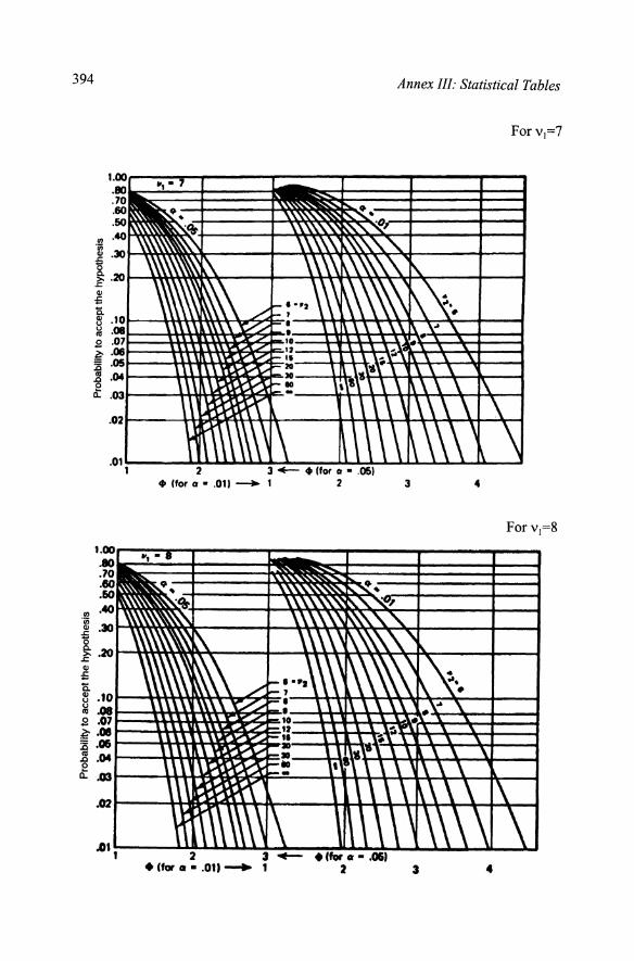
Table III.9. Curves of Constant Power for Test on Main Effects Forv1=1
3.5~ +(for Q a .05)
3 4 5
3 -+- +( for a • .051
+( for a • .011 - 1 2 3 4 5

392 Annex III: Statistical Tables
+C for ar • .01)--+- 1 4 5

Basics of Software Engineering Experimentation 393
.011 2
•ttor • • .OU __., 1 4 &
"' "ii
t ~~,~~~~~~~----~----~~~~~~~~~-----+----~ .s: .. =
2 3.-• ( for • • .011 __., 1 3 4
394 Annex III: Statistical Tables
2 41 (for a • .011 - 3 4
~tL,------~2LL~~~~~~~~~~~~~._._~--~
• (tor cr • .on --+ 3 4

Basics of Software Engineering Experimentation 395
Table 111.10. Wilcoxon Text
Test two tails one tail Test two tails one tail
n 5 % 1 % 0. 1 s 5 s 1 s n 5 s 1 s 0,1 s 5 l 1 s 6 0 2 36 208 171 130 227 185 7 2 3 0 37 221 182 140 241 198 8 3 0 5 1 38 235 194 150 256 211 9 5 1 8 3 39 249 207 161 271 224
10 8 3 10 5 40 264 220 172 286 238 11 10 5 0 13 7 41 279 233 183 302 252 12 13 7 1 17 9 42 294 247 195 319 266 13 17 9 2 21 12 43 310 261 207 336 281 14 21 12 4 25 15 44 327 276 220 353 296 15 25 15 6 30 19 45 343 291 233 371 312
16 29 19 8 35 23 46 361 307 246 389 328 17 34 23 11 41 27 47 378 322 260 407 345 18 40 27 14 47 32 48 396 339 274 426 362 19 46 32 18 53 37 49 415 355 289 446 379 20 52 37 21 60 43 50 434 373 304 466 397 21 58 42 25 67 49 51 45 3 390 319 486 416 22 65 48 30 75 55 52 473 408 335 507 434 23 73 54 35 83 62 53 494 427 351 529 454 24 81 61 40 91 69 54 514 445 368 550 473 25 89 68 45 100 76 55 5 36 465 385 I 573 493
26 98 75 51 110 84 56 557 484 402 595 514 27 107 83 57 119 92 57 579 504 420 618 535 28 116 91 64 130 101 58 602 525 438 642 556 29 126 100 71 140 110 59 625 546 457 666 578 30 137 109 78 151 120 60 648 567 476 690 600 31 14 7 118 86 163 130 61 672 589 495 715 623 32 159 128 94 175 140 62 697 611 515 741 646 33 170 138 102 187 151 63 721 634 535 767 669 34 182 148 111 200 162 64 747 657 556 793 693 35 195 159 120 213 173 65 772 681 577 820 718