references, pipelines & comparisons - stanford...
TRANSCRIPT

References, Pipelines &Comparisons
GenomicsGenetics 211 - Winter 2017
February 7, 2017
Mike Cherry

2
Number of regions with alternative loci or patches 234
Total sequence length 3,221,487,035
Total assembly gap length 160,028,125
Gaps between scaffolds 349
Number of scaffolds 766
Scaffold N50 67,794,873
Number of contigs 1,423
Contig N50 56,413,054
Total number of chromosomes and plasmids 25
Homo sapiens GRCh38

UCSC Version Release Date Release Namehg38 Dec 2013 GRCh38hg19 Feb 2009 GRCh37hg18 Mar 2006 NCBI Build 36.1hg17 May 2004 NCBI Build 35hg16 Jul 2003 NCBI Build 34hg15 Apr 2003 NCBI Build 33hg13 Nov 2002 NCBI Build 31hg12 Jun 2002 NCBI Build 30
…hg8 Aug 2001 UCSC assembled…
hg1 May 2000 UCSC assembled
Homo sapiens Reference Genome
GRC = Sanger, WashU, EBI and NCBI

hg19 (GRCh37) to GRCh38• Several thousand corrected bases in both
coding and non-coding regions• 100 assembly gaps closed or reduced• satellite repeat modeled
– megabase-sized gaps in centromere regions• updated mitochondrial reference sequence• many alternative reference sequences
– how to use in mapping?
4

5
HuRef
SOAPdenovo NA12878
ALLPATHS NA12878
MHAP CHM1
AK1HX1
Chaisson and Eichler (2015)

6
GRCh38 • 178 regions with alt loci: 2% of chromosome sequence (61.9 Mb) • 261 Alt Loci: 3.6 Mb novel sequence relative to chromosomes • Average alt length = 400 kb, max = ~5 Mb

7
GRCh38.p9 • 96 Patches: >1 Mb novel sequence • 48 FIX • 48 NOVEL

8
Previous GRC versions simply had a 3Mb gap on each chromosome to represent the centromeric region.
GRCh38 has a modeled the average centromere for human chromosomes
Karen Miga and Jim Kent, UCSC

Reference from a single individual
• GRCh38 is build from multiple individuals and from diploid sources, thus difficult to determine haploid context
• hydatidiform mole, haploid growth that forms inside the uterus at the beginning of a pregnancy
• Isolated by CHORI and BAC library CHORI-17 in 2002.
• Sanger, Illumina, PacBio, BioNano (optical)• GRC refers to this as the platinum genome• Others have build ancestry alternate SNP references
9

Transitioning between assemblies• UCSC liftOver software
– start with BED file– uses BLAT to identify matching regions, then alter the
coordinates– creates a chain file to defines the changes needed
between assemblies• NCBI Genome Remapping Service
– http://www.ncbi.nlm.nih.gov/genome/tools/remap
For processed data typically do not want to liftOver, rather remap and then rerun analysis.
10

11
Global Alliance for Genomics & Health (GA4GH)www.genomicsandhealth.org
http://ga4gh.org/

12B. Paten, A. Novak & D. Haussler. (2015) Mapping to a Reference Genome Structure. arXiv. 2014:1–26
One reference doesn’t fit all.

13
Single linear reference genome = “a single monoploid assembly of the genome of a species”
Can we do better?
How to better represent the sequence diversity and complexity?
More accurate sequence variant calling?
AM Novak, et al., 2017, https://doi.org/10.1101/101378
Genome Graphs

14B. Paten, A. Novak & D. Haussler. (2015) Mapping to a Reference Genome Structure. arXiv. 2014:1–26
Reference Genome in a Graph Representation

15B. Paten, A. Novak & D. Haussler. (2015) Mapping to a Reference Genome Structure. arXiv. 2014:1–26
Reference Genome in a Graph Representation

16AM Novak, et al., 2017, https://doi.org/10.1101/101378
Graph-based Variant Calling EvaluationShort Path Accuracy

17AM Novak, et al., 2017, https://doi.org/10.1101/101378
Variant Calling with Genome Graphs

blacklist & spongeRemoving regions of the genome that are associated with false positive signals.

19
• If the signal artifact (uniquely mapping) is extremely severe (>1000 fold) we flag the region.
• If the signal artifact is present in most of the tracks independent of cell-line or experiment type we flag the region.
• If the region has dispersed high mappability and low mappability coordinates then it is more likely to be an artifact region.
• If the region has a known repeat element then it is more likely to be an artifact• We check if the stranded read counts/signal is structured in the DNase, FAIRE
and input/control datasets, i.e. do we see offset mirror peaks on the + and - strand that is typical observed in real, functional peaks. If so we remove these regions from the artifact list.
• If the region exactly overlaps a known gene’s TSS, or is in the vicinity or within a known gene, it is more likely to be removed from the artifact list. Our intention is to give such regions the benefit of doubt of being real peaks.
Anshul Kundaje, 2014, A comprehensive collection of signal artifact blacklist regions in the human genome.https://docs.google.com/file/d/0B26FxqAtrFDwWGFCdXE1SlFYRmM/edit
https://www.encodeproject.org/annotations/ENCSR636HFF/
Blacklist for hg19

20Anshul Kundaje, 2014, A comprehensive collection of signal artifact blacklist regions in the human genome
Blacklist composition

21Anshul Kundaje, 2014, A comprehensive collection of signal artifact blacklist regions in the human genome
Signal due to unique mapping reads in high-mappability islands

22
Blacklist for GRCh38chr10 38528030 38529790chr10 42070420 42070660chr16 34571420 34571640chr16 34572700 34572930chr16 34584530 34584840chr16 34585000 34585220chr16 34585700 34586380chr16 34586660 34587100chr16 34587060 34587660chr16 34587900 34588170chr16 34593000 34593590chr16 34594490 34594720chr16 34594900 34595150chr16 34595320 34595570chr16 46380910 46381140chr16 46386270 46386530chr16 46390180 46390930chr16 46394370 46395100chr16 46395670 46395910chr16 46398780 46399020chr16 46400700 46400970
chr1 124450730 124450960chr20 28513520 28513770chr20 31060210 31060770chr20 31061050 31061560chr20 31063990 31064490chr20 31067930 31069060chr20 31069000 31069280chr21 8219780 8220120chr21 8234330 8234620chr2 90397520 90397900chr2 90398120 90398760chr3 93470260 93470870chr4 49118760 49119010chr4 49120790 49121130chr5 49601430 49602300chr5 49657080 49657690chr5 49661330 49661570
Anshul Kundaje (Stanford) & Alan Boyle (University of Michigan), October 2016

23K.H. Miga, C. Eisenhart and W.J. Kent. 2015. NAR doi:10.1093/nar/gkb671
sponge sequence database

24K.H. Miga, C. Eisenhart and W.J. Kent. 2015. NAR doi:10.1093/nar/gkb671

25K.H. Miga, C. Eisenhart and W.J. Kent. 2015. NAR doi:10.1093/nar/gkb671

pipelines

27http://www.nytimes.com/2016/02/05/science/dna-study-of-first-ancient-african-genome-flawed-researchers-report.html?_r=0
DNA Study of First Ancient African Genome Flawed, Researchers Report

28
Incompatible software
“Manica says that the error occurred when his team compared genetic variants in the ancient Ethiopian man with those in the reference
human genome. Incompatibility between the two software packages used caused some variants that the Ethiopian man shared with
Europeans (whose DNA forms a large chunk of the human reference sequence) to be removed from the analysis. This made Mota man seem less closely related to modern European populations than he
actually was — and in turn made contemporary African populations appear more closely related to Europeans. The researchers did have a
script that they could have run to harmonize the two software packages, says Manica, but someone forgot to run it.”
Ewen Callaway, January 29, 2016. Naturedoi:10.1038/nature.2016.19258

29

30
pipeline mistake
bwa ref.fasta sample[0-9].fastq > sample[0-9].bam
samtools mpileup -uf ref.fasta sample[0-9].bam | bcftools view -bvcg - > samples.raw.bcf
vcftools samples.vcf -plink samples
plink --file samples --genome
plink --file samples --read-genome samples.genome --cluster --mds-plot 2

31
“It’s so scary to work with this kind of data,” said Dr. Reich. “I’m sure we’ll make a mistake at some point, too.”
“That little oversight had a big impact. Dr. Manica and his colleagues unknowingly ignored some spots in the genome where Mota’s DNA was identical to that of Eurasians. As a result, Mota appeared not to be as closely related to Eurasians as he really was.
The mistake also created the false impression that many Africans outside of East Africa shared a lot of genes with Eurasians, DNA not found in Mota’s genome.”
Carl Zimmer, Feb 4, 2016 The New York Times

Nature feature: Challenges in irreproducible research
http://www.nature.com/news/reproducibility-1.17552
QC & measures of confidence
antibodies
standard & unique IDs
built in replication
data sharing

Data provenance & process transparency
DNase I
RNA-seq
DNase-seq
ChIP-seq
Bisulfite-seq
Processed data for further
analyses or visualization
?pipe
line
Avoid the pipeline blackbox

• ENCODE at UCSC’s Genome Browser • Roadmap at Baylor’s Genboree • IHEC at the IHEC Portal • Materials and Methods • Galaxy/Globus (Galaxy on the Cloud) • Seven Bridges Genomics • tarball of scripts • DNAnexus
sharing a pipeline
FASTQ (SE/PE)ReplicatesControls
Map ReadsFilterPool
SubsamplePseudoreplicates Call Peaks IDR
Signal Tracks
BAMReplicates
Pooled RepsControls
BAM2 Pseudoreplicates
per replicate2 Pseudoreplicates
per pool
peakReplicates
PseudoreplicatesPools
peakIDR-thresholded
Peak Calls
bigWigReplicates
Pooled Replicates
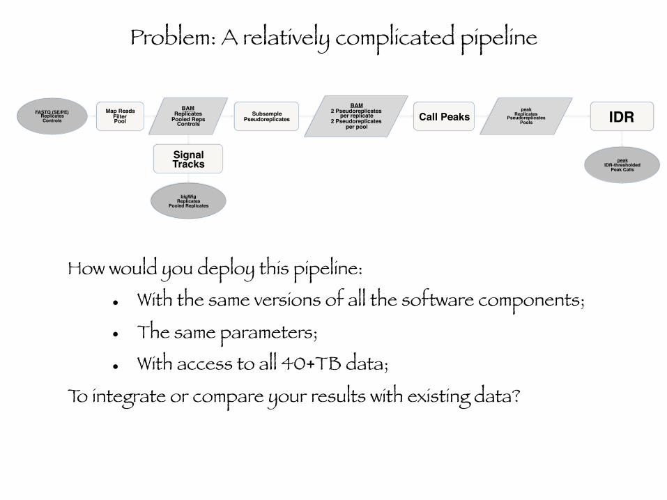
Problem: A relatively complicated pipeline
How would you deploy this pipeline:
• With the same versions of all the software components;
• The same parameters;
• With access to all 40+TB data;
To integrate or compare your results with existing data?

TF ChIP-seq processing pipeline
FASTQ (SE/PE)• Rep1 (Lane1)• Rep1 (Lane 2)• Rep2 (Lane1)• Rep2(Lane2)
Labs
1. Mapping (BWA)
BAM• Rep1• Rep2
1a. Mapping statistics1b. Library Complexity
2. Filter reads• Unmapped• Multimapping• Low Quality• Duplicates
BED•Rep1,•Rep2•Rep0 = Rep1+Rep2
2. Cross-correlation scores (NSC, RSC)
SubsampledPseudo-Replicates
• Rep1.pr1 , Rep1.pr2• Rep2.pr1, Rep2.pr2• Rep0.pr1, Rep0.pr2
3. Peak calling• SPP• GEM• PeakSeq
Relaxed Peak calls• Rep1 , Rep2• Rep0• Rep1.pr1, Rep2.pr2• Rep2.pr1, Rep2.pr2• Rep0.pr1, Rep0.pr2
5. Signal tracksChIP Fold-enrichment over
input
BIGWIG• Rep1• Rep2• Rep0
5. Signal Correlation between replicates
Files at DCC• FASTQs• BAM• QC measures• Peak calls• Signal tracks• Motifs
Processing Steps
QC
File Format
4. IDRIDR thresholds• Nt = Rep1 VS Rep2• Np = Rep0.pr1 VS Rep0.pr2• N1 = Rep1.pr1 VS Rep1.pr2• N2 = Rep2.pr1 VS Rep2.pr2• Optimal = max(Np,Nt)
4a. Self consistency ratio (N1/N2)4b. Rescue Ratio (Np/Nt)
Thresholded Peak calls (NarrowPeak)
• SPP (Blacklist filter)• GEM (Blacklist filter)• PeakSeq (Blacklist filter)
4c. Fraction of reads in Peaks (FRiP)
4d. Overlap between peak callers
6. Motif DiscoveryMotifs and motif hits
• Integrated GEM motifs• Post-peak calling motifs
Anshul Kundaje
TF ChIP-seq processing pipeline

J. Seth Strattan, PhD
Seven Bridges Genomics

What is Galaxy?
A collection of bioinformatics tools for: • data conversion and manipulation • statistical analysis • next generation sequencing analysis • provides integration of useful tools into
reuseable pipelines, that can also be shared • unified and consistent interface for easy
exploration
Toolbox for: • retrieving (“get”) data • manipulating data (liftOver, filter, sort, set
operations, format conversion) • data analysis (statistics, sequence alignment,
variant calling and annotation)

dozens of tools for different NGS applications packaged with Galaxy

Galaxy pipelines
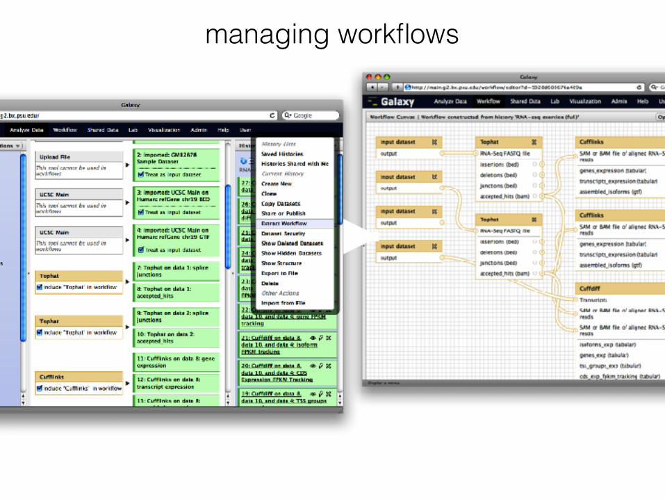
managing workflows
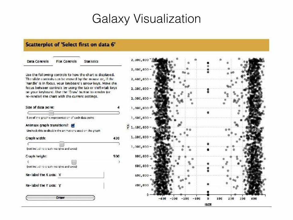
Galaxy Visualization

DNA nexus pipeline form
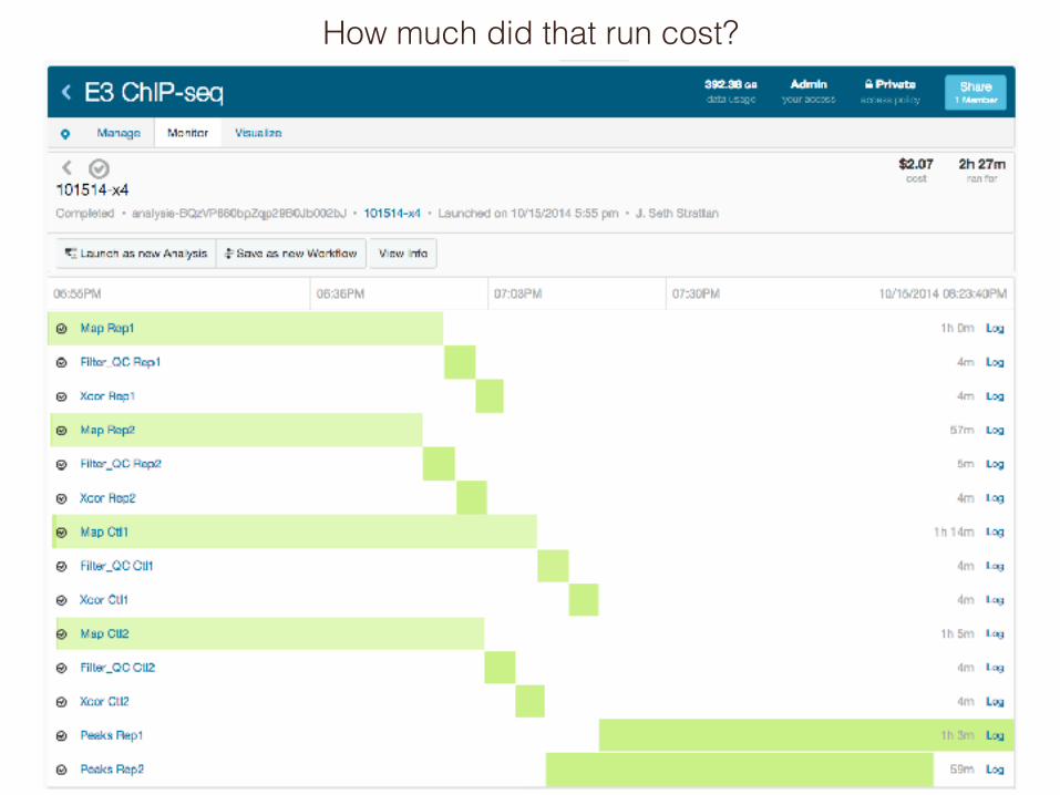
How much did that run cost?

45
examples of large commercial cloud service providers
Amazon Web Services http://aws.amazon.com/Google Cloud Platform https://cloud.google.com/Microsoft Azure http://www.azure.microsoft.com/IBM Cloud http://www.ibm.com/cloud-computingHP Public Cloud http://www.hpcloud.com/Citrix CloudPlatform https://www.citrix.com/products/cloudplatform/
overview.htmlRackspace Cloud http://www.rackspace.com/cloud/

Sequence Comparison

Goals of Sequence Comparison:
• Find similarity such that an inference of homology is justified. – Similarity = observed with sequence alignment – Homology = shared evolutionary history
(ancestry) • Find a new sequence (gene) of interest • Provide biologically appropriate results.
– Substitutions, insertions and deletions • Compare as many sequences as fast as
possible.
47

Local vs. Global Alignment
• Global Alignment
• Local Alignment—better alignment to find conserved segment
--T—-CC-C-AGT—-TATGT-CAGGGGACACG—A-GCATGCAGA-GAC | || | || | | | ||| || | | | | |||| | AATTGCCGCC-GTCGT-T-TTCAG----CA-GTTATG—T-CAGAT--C
tccCAGTTATGTCAGgggacacgagcatgcagagac ||||||||||||aattgccgccgtcgttttcagCAGTTATGTCAGatc
48

Dynamic Programming Basics for sequence alignment. Smith-Waterman method.
Scoring for nucleotides: Match = 2 Gap = -1 Mismatch = -1
Use scores to complete the matrix, row by row. Add, or subtract, from neighboring cell with the highest score using this order:
1) diagonal 2) right 3) up
CA
CA2 2-1=1
2-1=1 2+2=4
49

50
- T A C T A A C G C
- 0 0 0 0 0 0 0 0 0 0
A 0 0 2 1 0 2 2 1 0 0
C
A
C
G
C
T
Points: match +2, mismatch or gap -1 Order: Diagonal, left, up

51
- T A C T A A C G C
- 0 0 0 0 0 0 0 0 0 0
A 0 0 2 1 0 2 2 1 0 0
C 0 0 1 4 3 1 1 4 3 2
A 0 0 2 3 2 5 3 3 2 1
C
G
C
T
Points: match +2, mismatch or gap -1 Order: Diagonal, left, up

52
- T A C T A A C G C
- 0 0 0 0 0 0 0 0 0 0
A 0 0 2 1 0 2 2 1 0 0
C 0 0 1 4 3 1 1 4 3 2
A 0 0 2 3 2 5 3 3 2 1
C 0 0 1 4 1 4 2 5 1 4
G 0 0 0 3 0 3 1 4 7 3
C
T
Points: match +2, mismatch or gap -1 Order: Diagonal, left, up

53
- T A C T A A C G C
- 0 0 0 0 0 0 0 0 0 0
A 0 0 2 1 0 2 2 1 0 0
C 0 0 1 4 3 1 1 4 3 2
A 0 0 2 3 2 5 3 3 2 1
C 0 0 1 4 1 4 2 5 1 4
G 0 0 0 3 0 3 1 4 7 3
C 0 0 0 2 1 2 0 3 6 9
T 0 0 0 1 4 1 0 2 5 8
Points: match +2, mismatch or gap -1 Order: Diagonal, left, up

54
- T A C T A A C G C
- 0 0 0 0 0 0 0 0 0 0
A 0 0 2 1 0 2 2 1 0 0
C 0 0 1 4 3 1 1 4 3 2
A 0 0 2 3 2 5 3 3 2 1
C 0 0 1 4 1 4 2 5 1 4
G 0 0 0 3 0 3 1 4 7 3
C 0 0 0 2 1 2 0 3 6 9
T 0 0 0 1 4 1 0 2 5 8
Points: match +2, mismatch or gap -1 Order: Diagonal, left, up
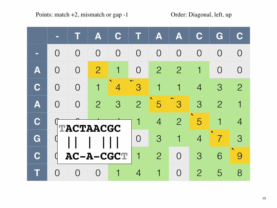
55
- T A C T A A C G C
- 0 0 0 0 0 0 0 0 0 0
A 0 0 2 1 0 2 2 1 0 0
C 0 0 1 4 3 1 1 4 3 2
A 0 0 2 3 2 5 3 3 2 1
C 0 0 1 4 1 4 2 5 1 4
G 0 0 0 3 0 3 1 4 7 3
C 0 0 0 2 1 2 0 3 6 9
T 0 0 0 1 4 1 0 2 5 8
Points: match +2, mismatch or gap -1 Order: Diagonal, left, up
TACTAACGC || | ||| AC-A-CGCT

Scoring Matrix
• Modeled Change in Protein Sequences – PAM (Accepted Point Mutations) – Schwartz & Dayhoff (1978)
• Experimentally Derived Matrix – BLOSUM (BLOCKS Substitution Matrix) – Henikoff & Henikoff (1992)
56

• Number of individual amino acid changes occurring per 100 aa residues as a result of evolution. PAM1 = unit of evolutionary divergence in which 1% of the amino acids have been changed.
• PAM of 250, or PAM250, represents [PAM1]250. The PAM1 matrix multiplied against itself 250 times.
Accepted Point Mutations (PAM) or Percent Accepted Mutations
57

Creating the PAM1 Schwartz & Dayhoff (1978)
• Studied 34 protein super-families and grouped them into 71 phylogenetic trees. There were 1,572 changes observed. All sequences were at least 85% identical. Alignments were scanned with a 100 amino acid window.
• These are observed mutations thus the term accepted point mutations, accepted by natural selection and thus the dominant allele in the species.
• Normalized probability of change: Pij = (Cij / T) x (1 / Fi) Cij = number of changes from aai to aaj Fi = freq of aai in that group of sequences T = total number of all aa changes in 100 sites
58

A 2
R -2 6
N 0 0 2
D 0 -1 2 4
C -2 -4 -4 -5 12
Q 0 1 1 2 -5 4
E 0 -1 1 3 -5 2 4
G 1 -3 0 1 -3 -1 0 5
H -1 2 2 1 -3 3 1 -2 6
I -1 -2 -2 -2 -2 -2 -2 -3 -2 5
L -2 -3 -3 -4 -6 -2 -3 -4 -2 -2 6
K -1 3 1 0 -5 1 0 -2 0 -2 -3 5
M -1 0 -2 -3 -5 -1 -2 -3 -2 2 4 0 6
F -3 -4 -3 -6 -4 -5 -5 -5 -2 1 2 -5 0 9
P 1 0 0 -1 -3 0 -1 0 0 -2 -3 -1 -2 -5 6
S 1 0 1 0 0 -1 0 1 -1 -1 -3 0 -2 -3 1 2
T 1 -1 0 0 -2 -1 0 0 -1 0 -2 0 -1 -3 0 1 3
W -6 2 -4 -7 -8 -5 -7 -7 -3 -5 -2 -3 -4 0 -6 -2 -5 17
Y -3 -4 -2 -4 0 -4 -4 -5 0 -1 -1 -4 -2 7 -5 -3 -3 0 10
V 0 -2 -2 -2 -2 -2 -2 -1 -2 4 2 -2 2 -1 -1 -1 0 -6 -2 4
A R N D C Q E G H I L K M F P S T W Y V
PAM250 log oddsscoring matrix
59

Protein family 1 x 10⁷ (PAM)Immunoglobulin (Ig) kappa chain 37
Kappa casein 33
Luteinizing hormone b 30
Lactalbumin 27
Complement component 3 27
Collagen 1.7
Troponon C, skeletal muscle 1.5
Alpha crystallin B chain 1.5
Glucagon 1.2
Glutamate dehydrogenase 0.9
Histone H2B, member Q 0.9
Ubiquitin 0
From Dayhoff (1978)
60

Per
cent
iden
tity
Differences per 100 residues
“twilight zone”
PAM1 99% identity PAM10.7 90% identity PAM80 50% identity PAM250 20% identity
Perc
ent I
den
tity
61

Deriving Substitution Scores BLOSUMHenikoff & Henikoff, 1992
Protein Family
Block A Block B
62

63
BLOSUM 62 scoring matrix

64ftp://ftp.ncbi.nlm.nih.gov/pub/factsheets/HowTo_BLASTGuide.pdf
NCBI BLAST
Getting Started with BLAST handout:
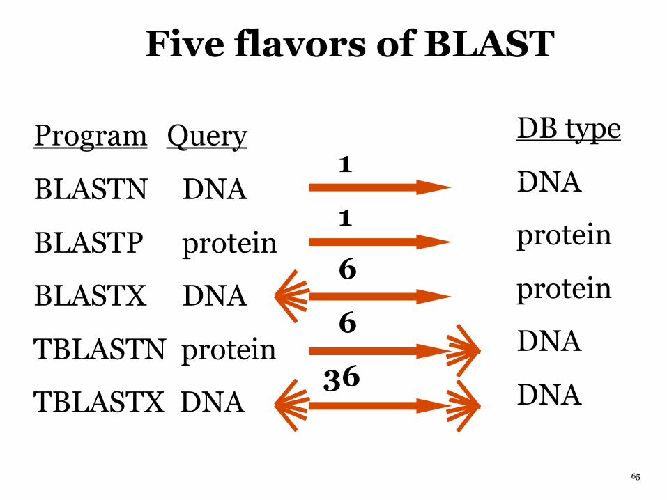
Five flavors of BLAST
Program Query 1BLASTN DNA 1BLASTP protein 6BLASTX DNA 6TBLASTN protein 36TBLASTX DNA
DB type
DNA
protein
protein
DNA
DNA
65

query word (W=3)
Query: GSVEDTTGSQSLAALLNKCKTPQGQRLVNQWIKQPLMDKNRIEERLNLVEAFVEDAELRQTLQEDL
PQG 17 PEG 14 PRG 13 PKG 13 PNG 12 PDG 12 PHG 12 PMG 12 PSG 12 PQN 11 PQA 10 etc ...
Query: 325 SLAALLNKCKTPQGQRLVNQWIKQPLMDKNRIEERLNLVEA 365 +LA++L+ TP G R++ +W+ P+ D + ER + ASbjct: 290 TLASVLDCTVTPKGSRMLKRWLHMPVRDTRVLLERQQTIGA 330
High-scoring Segment Pair (HSP)
The BLAST Search Algorithm
neighborhoodscore threshold(T = 13)
neighborhoodwords
(from NCBI Web site) 66

67Kerfeld and Scott, PLoS Biology 2011
Raw Scores (S values) from an Alignment
S = (ΣMij) – cO – dG, where M = score from a similarity matrix for a particular pair of amino acids (ij) c = number of gaps O = penalty for the existence of a gap d = total length of gaps G = per-residue penalty for extending
the gap
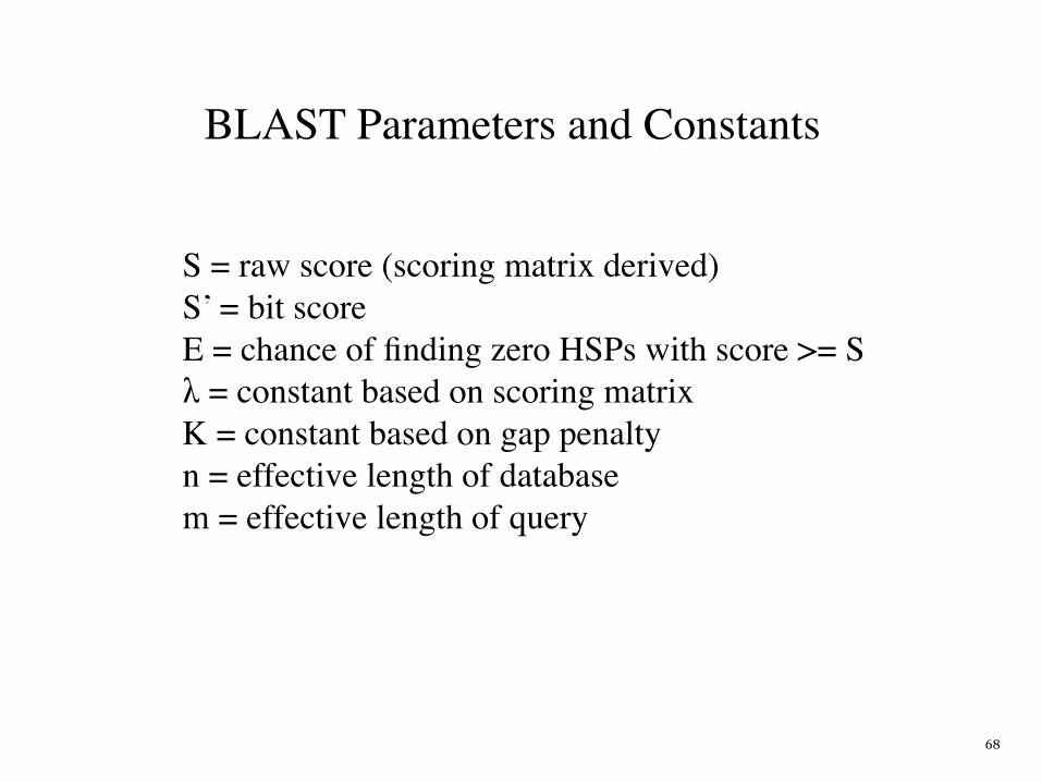
BLAST Parameters and Constants
S = raw score (scoring matrix derived)S’ = bit scoreE = chance of finding zero HSPs with score >= Sλ = constant based on scoring matrixK = constant based on gap penaltyn = effective length of databasem = effective length of query
68
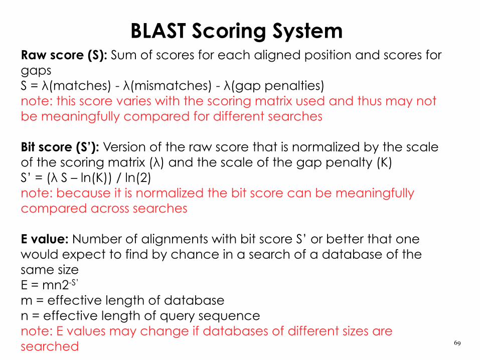
Raw score (S): Sum of scores for each aligned position and scores for gaps S = λ(matches) - λ(mismatches) - λ(gap penalties) note: this score varies with the scoring matrix used and thus may not be meaningfully compared for different searches
Bit score (S’): Version of the raw score that is normalized by the scale of the scoring matrix (λ) and the scale of the gap penalty (K) S’ = (λ S – ln(K)) / ln(2) note: because it is normalized the bit score can be meaningfully compared across searches
E value: Number of alignments with bit score S’ or better that one would expect to find by chance in a search of a database of the same size E = mn2-S’ m = effective length of database n = effective length of query sequence note: E values may change if databases of different sizes are searched
BLAST Scoring System
69

70
BLAST report
m

71
Smart BLASTBLASTP + COBALT MSA
Yellow - Query SequenceGreen - Landmark Databases of 27 genomes spanning a wide taxonomic rangeGray - Region not aligned to Query by BLASTWhite - Region not aligned by COBALT
COBALT

• BLAT is designed to find sequences of >95% similarity of length >40 bases. Perfect sequence matches of >33 bases are identified.
• Protein BLAT finds sequences of >80% similarity of length >20 amino acids.
• DNA BLAT works by keeping an index of the entire genome. The index consists of all non-overlapping 11-mers except for those in repeats.
• Protein BLAT works in a similar manner, except with 4-mers rather than 11-mers.
• The index is used to find areas of probable similarity. Then the sequence for the area of interest is read into memory for a detailed alignment.
BLAT -- BLAST-Like Alignment Tool By Jim Kent, UCSC
http://genome.ucsc.edu/cgi-bin/hgBlat
72

73
BLAT Indexing

BLAT output includes browser and other formats
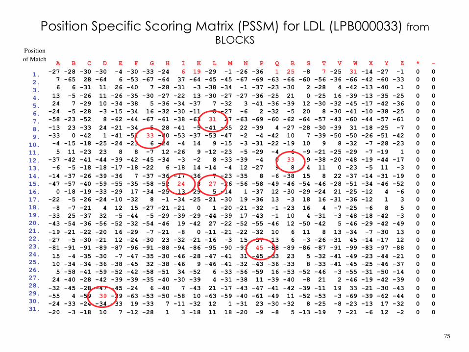
A B C D E F G H I K L M N P Q R S T V W X Y Z * --27 -28 -30 -30 -4 -30 -33 -24 6 19 -29 -1 -26 -36 1 25 -8 7 -25 31 -14 -27 -1 0 0 7 -65 28 -64 6 -53 -67 -64 37 -64 -45 -45 -67 -69 -63 -66 -60 -56 -36 -66 -42 -60 -33 0 0 6 6 -31 11 26 -40 7 -28 -31 -3 -38 -34 -1 -37 -23 -30 2 -28 4 -42 -13 -40 -1 0 0 13 -5 -26 11 -26 -35 -30 -27 -22 13 -30 -27 -27 -36 -25 21 0 -25 16 -39 -13 -35 -25 0 0 24 7 -29 10 -34 -38 5 -36 -34 -37 7 -32 3 -41 -36 -39 12 -30 -32 -45 -17 -42 -36 0 0-24 -5 -28 -3 -15 -34 16 -32 -30 -11 8 -27 -6 2 -32 -5 20 8 -30 -41 -10 -38 -25 0 0-58 -23 -52 8 -62 -44 -67 -61 -38 -63 31 27 -63 -69 -60 -62 -64 -57 -43 -60 -44 -57 -61 0 0-13 23 -33 24 -21 -34 5 28 -41 -5 -41 -35 22 -39 4 -27 -28 -30 -39 31 -18 -25 -7 0 0-33 0 -42 1 -41 -51 33 -40 -53 -37 -53 -47 -2 -4 -42 10 7 -39 -50 -50 -26 -51 -42 0 0 -4 -15 -18 -25 -24 -23 6 -24 -4 14 9 -15 -3 -31 -22 -19 10 9 8 -32 -7 -28 -23 0 0 5 11 -23 23 8 8 -7 12 -26 9 -12 -23 -5 -29 -4 6 -9 -21 -25 -29 -7 -19 1 0 0-37 -42 -41 -44 -39 -42 -45 -34 -3 -2 8 -33 -39 -4 0 33 9 -38 -20 -48 -19 -44 -17 0 0 -6 -5 -18 -18 -17 -18 -22 6 -18 14 -14 -4 12 -27 9 8 4 11 0 -23 -5 11 -3 0 0-14 -37 -26 -39 -36 7 -37 -36 -17 -36 7 -23 -35 8 -6 -38 15 8 22 -37 -14 -31 -19 0 0-47 -57 -40 -59 -55 -35 -58 -52 24 8 27 -26 -56 -58 -49 -46 -54 -46 -28 -51 -34 -46 -52 0 0 0 -18 -19 -33 -29 17 -34 -25 13 -29 5 -14 1 -37 12 -30 -29 -24 21 -25 -12 4 -6 0 0-22 -5 -26 -24 -10 -32 8 -1 -34 -25 -21 -30 19 -36 13 -3 18 16 -31 -36 -12 1 3 0 0 -8 -7 -21 4 12 15 -27 -21 -21 0 1 -20 -21 -32 -1 -23 16 4 -7 -25 -6 8 5 0 0-33 25 -37 32 -5 -44 -5 -29 -39 -29 -44 -39 17 -43 -1 10 4 -31 -3 -48 -18 -42 -3 0 0-43 -54 -36 -56 -52 -32 -54 -46 19 -42 27 -22 -52 -55 -46 12 -50 -42 5 -46 -29 -42 -49 0 0-19 -21 -22 -20 16 -29 -7 -21 -8 0 -11 -21 -22 -32 10 6 11 8 13 -34 -7 -30 13 0 0-27 -5 -30 -21 12 -24 -30 23 -32 -21 -16 -3 15 -37 13 6 -3 -26 -31 45 -14 -17 12 0 0-81 -91 -91 -89 -87 -96 -91 -88 -94 -86 -95 -90 -93 45 -88 -89 -86 -87 -91 -99 -83 -97 -88 0 0 15 -4 -35 -30 -7 -47 -35 -30 -46 -28 -47 -41 31 -45 -33 23 5 -32 -41 -49 -23 -44 -21 0 0 10 -34 -34 -36 -38 -45 32 -38 -46 9 -46 -41 -32 -43 -36 -33 8 -33 -41 -45 -25 -46 -37 0 0 5 -58 -41 -59 -52 -42 -58 -51 34 -52 6 -33 -56 -59 16 -53 -52 -46 -3 -55 -31 -50 -14 0 0 24 -40 -28 -42 -39 -39 -35 -40 -30 -39 4 -31 -38 11 -39 -40 -8 21 2 -46 -19 -42 -39 0 0-32 -45 -28 -47 -45 -24 6 -40 7 -43 21 -17 -43 -47 -41 -42 -39 -11 19 33 -21 -30 -43 0 0-55 4 -59 39 -39 -63 -53 -50 -58 10 -63 -59 -40 -61 -49 11 -52 -53 -3 -69 -39 -62 -44 0 0-24 -33 -24 -34 -33 19 -33 7 -11 -32 12 1 -31 23 -30 -32 8 -25 -8 -23 -13 17 -32 0 0-20 -3 -18 10 7 -12 -28 1 3 -18 11 18 -20 -9 -8 5 -13 -19 7 -21 -6 12 -2 0 0
Position Specific Scoring Matrix (PSSM) for LDL (LPB000033) from BLOCKS
1.2.3.4.5.6.7.8.9.
10.11.12.13.14.15.16.17.18.19.20.21.22.23.24.25.26.27.28.29.30.31.
Positionof Match
75

Logos provide a simple visualization of a PSSM
Crooks GE, Hon G, Chandonia JM, Brenner SE. 2004. WebLogo: A sequence logo generator. Genome Res., 14:1188-1190 [weblogo.berkeley.edu]
Schneider TD, Stephens RM. 1990. Sequence Logos: A New Way to Display Consensus Sequences. Nucleic Acids Res. 18:6097-6100
76

Considerations when making a profile.
• How are missing sequences represented? • Many sequences are needed to create a
useful alignment, but not too many that are closely related.
• Where are the gaps located?
77

• Rosenbloom, KR, et al., (2015) The UCSC Genome Browser database : 2015 update
• Korf, Yandell & Bedell (2003) BLAST: An Essential Guide to the Basic Local Alignment Search Tool. O’Reilly
• Jonathan Pevsner (2003) Bioinformatics and Functional Genomics. Wiley-Liss
• Mount (2004) Bioinformatics: Sequence and Genome Analysis. Cold Spring Harbor Laboratory Press
• Baxevanis & Ouellette (2001) Bioinformatics: A Practical Guide to the Analysis of Genes and Proteins. Wiley Interscience
• Jones & Pevzner (2004) An Introduction to Bioinformatic Algorithms. (MIT Press)
• Salzberg, Searls & Kasif (1998) Computational Methods in Molecular Biology. Elsevier
• Waterman (1995) Introduction to Computation Biology.
Reading
78