redundancy investments in manufacturing systems
TRANSCRIPT

Redundancy Investments inManufacturing Systems
The role of redundancies for manufacturing system robustness
by
Dipl.-Wi.-Ing. Mirja Meyer
A Thesis submitted in partial fulfillment of the requirements for the degree of
Doctor of Philosophyin International Logistics
Approved dissertation committee:
Prof. Dr. Julia Bendul (chair, Jacobs University)Prof. Dr. Marc-Thorsten Hütt (Jacobs University)Prof. Dr.-Ing. Michael Freitag (Universität Bremen)
Date of defense: 12.10.2016
Department of Mathematics & Logistics


Abstract
Today’s manufacturing companies are faced with a large number of fluctuatinginfluence factors, as supply chains in the production environment grow larger withmore suppliers and highly sophisticated products. At the same time, throughput timesand due date reliability need to stay on a stable level, to fulfill the expectations of shortdelivery times and high service-levels of increasingly demanding customers. This abilityto maintain specific features or a certain performance when subject to fluctuations anddisturbances is generally referred to as robustness. As explained above, robustness ofperformance indicators, such as due date reliability, is a desirable characteristic forproducing companies, hence the question arises how it can be achieved or incorporatedin a companies manufacturing system. Looking at other scientific disciplines, such asbiology or complex network science, robustness of the respective systems is often causedby redundancy, a situation where identical or similar components can replace eachother when a component fails. In manufacturing research, redundancy has often beenconsidered as an aspect to be avoided, as it stands in a potential trade-off with cost-efficiency, for example in lean manufacturing where excess inventory is considered aswaste. However, as redundancy has been shown to have a strong relation to robustnessin other disciplines, the aim of this thesis is to investigate the role that redundancyplays for achieving robustness of manufacturing system performance. In a first step,definitions from literature for both robustness and redundancy are reviewed, with aparticular focus on approaches from biology, as the robustness-redundancy relationhas attracted a lot of attention in this domain. Definitions for both robustness andredundancy are then derived for a manufacturing context. In addition to these measuresbased on a manufacturing background, two indicators usually used in a biologicalcontext for the analysis of robustness and redundancy, nestedness and elementaryflux modes, are considered for measurement of redundancy in manufacturing systems.Using a discrete-event simulation, the relationship between both constructs - robustnessand redundancy - is analyzed for a large-scale of different manufacturing systemconfigurations. It is found that both a redundancy indicator derived from a classicalmanufacturing background, but also elementary flux modes derived from systemsbiology, are significantly correlated with robustness of performance in manufacturingsystems. In a final step, it is presented how the findings of the relationship betweenrobustness and redundancy can be applied to incorporate robustness into the design ofmanufacturing systems.
i

Contents
List of Abbreviations v
List of Figures vi
List of Tables viii
1 Introduction 11.1 Problem formulation and motivation . . . . . . . . . . . . . . . . . . . . . . 11.2 Research questions and scope . . . . . . . . . . . . . . . . . . . . . . . . . . 51.3 Research approach and thesis outline . . . . . . . . . . . . . . . . . . . . . . 6
2 Related Work 82.1 Introduction to manufacturing systems . . . . . . . . . . . . . . . . . . . . . 8
2.1.1 Definition and terms of manufacturing systems . . . . . . . . . . . . 82.1.2 Objectives, trade-offs, and performance in manufacturing systems . . 112.1.3 Manufacturing systems design . . . . . . . . . . . . . . . . . . . . . . 152.1.4 Negative influence of complexity and disturbances on manufacturing
system performance . . . . . . . . . . . . . . . . . . . . . . . . . . . 212.2 Robustness definitions, measures, and disambiguation in manufacturing
systems . . . . . . . . . . . . . . . . . . . . . . . . . . . . . . . . . . . . . . 232.2.1 Robustness as a general system characteristic . . . . . . . . . . . . . 232.2.2 Robustness definitions and measures in manufacturing systems . . . 242.2.3 Robust manufacturing system design . . . . . . . . . . . . . . . . . . 262.2.4 Concepts similar to robustness in manufacturing systems research . 282.2.5 Redundancy as a general system characteristic . . . . . . . . . . . . 292.2.6 Redundancy in safety and reliability engineering . . . . . . . . . . . 292.2.7 Redundancy definitions and measures in manufacturing systems . . 30
2.3 Complex networks and bio-inspired approaches in manufacturing systemsresearch . . . . . . . . . . . . . . . . . . . . . . . . . . . . . . . . . . . . . . 302.3.1 Motivation for interdisciplinary research in manufacturing systems
research . . . . . . . . . . . . . . . . . . . . . . . . . . . . . . . . . . 302.3.2 Complex network science and manufacturing systems . . . . . . . . 322.3.3 Biological systems and manufacturing systems . . . . . . . . . . . . 38
2.4 Research Gap . . . . . . . . . . . . . . . . . . . . . . . . . . . . . . . . . . . 452.4.1 Lack of robustness considerations in the design of manufacturing
systems . . . . . . . . . . . . . . . . . . . . . . . . . . . . . . . . . . 452.4.2 Influence of redundancy on the robustness of manufacturing system
performance . . . . . . . . . . . . . . . . . . . . . . . . . . . . . . . . 452.4.3 Motivation for using interdisciplinary methods for robust manufac-
turing systems design . . . . . . . . . . . . . . . . . . . . . . . . . . 46
ii

Contents
3 Analyzing the relationship between robustness and redundancy in MSs 473.1 Defining and measuring robustness in manufacturing systems . . . . . . . . 483.2 Defining and measuring redundancy in job shop manufacturing systems . . 503.3 Potential relationship between robustness and redundancy . . . . . . . . . . 533.4 Simulation analysis of the relation between redundancy and robustness in MSs 55
3.4.1 Simulation as a research methodology in manufacturing systemsresearch . . . . . . . . . . . . . . . . . . . . . . . . . . . . . . . . . . 55
3.4.2 Configuration of realistic exemplary manufacturing systems . . . . . 573.4.3 Simulation model description and discussion of results . . . . . . . . 633.4.4 Correlating robustness, redundancy, and complex network measures 67
3.5 Summary of intermediary results . . . . . . . . . . . . . . . . . . . . . . . . 69
4 Analyzing nestedness of the part-resources network in manufacturing systems 714.1 Nestedness concept and metrics . . . . . . . . . . . . . . . . . . . . . . . . . 724.2 Application of nestedness analysis in ecological and non-ecological systems . 774.3 Modeling manufacturing systems as mutualistic networks . . . . . . . . . . 784.4 Application of nestedness analysis to a case study manufacturing system . . 80
4.4.1 Description of the analyzed system . . . . . . . . . . . . . . . . . . . 804.4.2 Nestedness calculation and discussion of results . . . . . . . . . . . . 81
4.5 Application of nestedness analysis to the test manufacturing system config-urations . . . . . . . . . . . . . . . . . . . . . . . . . . . . . . . . . . . . . . 824.5.1 Nestedness calculation and discussion of results . . . . . . . . . . . . 824.5.2 Correlating robustness and nestedness . . . . . . . . . . . . . . . . . 84
4.6 Summary of intermediary results . . . . . . . . . . . . . . . . . . . . . . . . 85
5 Analyzing elementary flux modes in the resources-material flow network in MSs 875.1 Elementary flux mode analysis in metabolic networks . . . . . . . . . . . . . 885.2 Modeling manufacturing systems as metabolic networks . . . . . . . . . . . 905.3 Application of elementary flux mode analysis to a case study manufacturing
system . . . . . . . . . . . . . . . . . . . . . . . . . . . . . . . . . . . . . . . 925.3.1 Description of the analyzed system . . . . . . . . . . . . . . . . . . . 925.3.2 Elementary flux mode calculation and discussion of results . . . . . 935.3.3 Machine knock-out study and discussion of results . . . . . . . . . . 945.3.4 Correlation of elementary flux modes and manufacturing performance
indicators . . . . . . . . . . . . . . . . . . . . . . . . . . . . . . . . . 955.4 Application of elementary flux mode analysis to the test MS configurations 100
5.4.1 Elementary flux mode calculation and discussion of results . . . . . 1005.4.2 Machine knockout study and discussion of results . . . . . . . . . . . 1015.4.3 Correlation of robustness and elementary flux modes . . . . . . . . . 102
5.5 Summary of intermediary results . . . . . . . . . . . . . . . . . . . . . . . . 103
6 Designing robust manufacturing systems with redundancy considerations 1056.1 Potential use of structural redundancy measures in MSD procedures . . . . 1056.2 Considering the trade-off between redundancy-induced robustness and cost-
efficiency . . . . . . . . . . . . . . . . . . . . . . . . . . . . . . . . . . . . . . 1086.3 Discussion of the use of structural redundancy indicators for RMSD . . . . 1116.4 Summary of intermediary results . . . . . . . . . . . . . . . . . . . . . . . . 113
7 Conclusion 1157.1 Summary of results . . . . . . . . . . . . . . . . . . . . . . . . . . . . . . . . 115
iii

Contents
7.2 Assumptions and limitations . . . . . . . . . . . . . . . . . . . . . . . . . . 1177.3 Implications for industry . . . . . . . . . . . . . . . . . . . . . . . . . . . . . 1187.4 Outlook on further research . . . . . . . . . . . . . . . . . . . . . . . . . . . 118
Bibliography 119
Appendix 149
Declaration 159
iv

List of Abbreviations
BOM Bill Of Material
DES Discrete-Event Simulation
EFM Elementary Flux Mode
FBA Flux Balance Analysis
FMS Flexible Manufacturing System
MS Manufacturing System
MSD Manufacturing Systems Design
MSP Manufacturing System Performance
NTC Nestedness Temperature Calculator
RMSD Robust Manufacturing Systems Design
T Nestedness Temperature
WIP work in process
v

List of Figures
1.1 Influence of structural and dynamic complexity on manufacturing systemperformance . . . . . . . . . . . . . . . . . . . . . . . . . . . . . . . . . . . . 2
1.2 Thesis outline, research methods, and objectives . . . . . . . . . . . . . . . 7
2.1 Definition of a manufacturing system with its inputs and outputs . . . . . . 92.2 Exemplary types of manufacturing systems . . . . . . . . . . . . . . . . . . 112.3 Suitability of manufacturing system type depending on product variety and
volume . . . . . . . . . . . . . . . . . . . . . . . . . . . . . . . . . . . . . . . 122.4 Hierarchical objectives in a manufacturing organization . . . . . . . . . . . 132.5 The manufacturing tetrahedron . . . . . . . . . . . . . . . . . . . . . . . . . 142.6 The manufacturing control dilemma . . . . . . . . . . . . . . . . . . . . . . 142.7 Decision horizons in manufacturing systems . . . . . . . . . . . . . . . . . . 152.8 Relation between product design and resource design . . . . . . . . . . . . . 162.9 Conceptual representations of trade-off curves between resource costs and
WIP costs . . . . . . . . . . . . . . . . . . . . . . . . . . . . . . . . . . . . . 202.10 Classification of disturbances in MSs . . . . . . . . . . . . . . . . . . . . . . 222.11 Type I and II robustness in robust design . . . . . . . . . . . . . . . . . . . 282.12 Exemplary graphs and adjacency matrices . . . . . . . . . . . . . . . . . . . 332.13 Exemplary bipartite graph and adjacency matrix . . . . . . . . . . . . . . . 342.14 Node degrees of exemplary graphs . . . . . . . . . . . . . . . . . . . . . . . 342.15 Shortest paths and network diameter . . . . . . . . . . . . . . . . . . . . . . 352.16 Exemplary betweenness centrality calculation . . . . . . . . . . . . . . . . . 362.17 Three different ways to model metabolic networks . . . . . . . . . . . . . . 392.18 Similarities between manufacturing and metabolic systems . . . . . . . . . . 402.19 Comparison of redundancy and functional redundancy . . . . . . . . . . . . 44
3.1 Conceptual depiction of MSP in a MS . . . . . . . . . . . . . . . . . . . . . 493.2 Different types of lateness . . . . . . . . . . . . . . . . . . . . . . . . . . . . 493.3 Conceptual depiction of the potential relationship between robustness and
redundancy in MSs . . . . . . . . . . . . . . . . . . . . . . . . . . . . . . . . 543.4 Number of machines per MS configuration . . . . . . . . . . . . . . . . . . . 603.5 Redundancy in the MS configurations . . . . . . . . . . . . . . . . . . . . . 613.6 Complex network measures in the MS configurations . . . . . . . . . . . . . 633.7 Robustness values of the 81 MS configuration . . . . . . . . . . . . . . . . . 663.8 Relation of robustness and redundancy . . . . . . . . . . . . . . . . . . . . . 683.9 Relation of robustness and complex network measures in MSs . . . . . . . . 69
4.1 Schematic representation of nestedness . . . . . . . . . . . . . . . . . . . . . 724.2 Nested structure of a matrix . . . . . . . . . . . . . . . . . . . . . . . . . . . 734.3 Shuffling of an observed presence-absence matrix . . . . . . . . . . . . . . . 744.4 Measuring unexpectedness in an examplary matrix . . . . . . . . . . . . . . 74
vi

List of Figures
4.5 Exemplary calculation of NODF . . . . . . . . . . . . . . . . . . . . . . . . 764.6 Bipartite system depictions . . . . . . . . . . . . . . . . . . . . . . . . . . . 794.7 Creation of a part-resource matrix . . . . . . . . . . . . . . . . . . . . . . . 794.8 Machines and material flows in the analyzed job shop . . . . . . . . . . . . 814.9 Nested matrix of the parts-resources matrix of the analyzed company . . . 824.10 Nestedness values of the 81 MSconfigurations . . . . . . . . . . . . . . . . . 834.11 Relation of robustness and nestedness . . . . . . . . . . . . . . . . . . . . . 85
5.1 Metabolic network modeling . . . . . . . . . . . . . . . . . . . . . . . . . . . 885.2 EFMs of a metabolic reaction network . . . . . . . . . . . . . . . . . . . . . 895.3 Product structure and route sheets for an exemplary product . . . . . . . . 915.4 Modeling machine-material flow networks as metabolic networks . . . . . . 915.5 Analyzed real case data . . . . . . . . . . . . . . . . . . . . . . . . . . . . . 925.6 Number of EFMs per time bin . . . . . . . . . . . . . . . . . . . . . . . . . 935.7 Average percentage of EFMs that are deleted if a machine is not available . 955.8 Correlations of different indicators with average machine lateness . . . . . . 975.9 Correlations of the different indicators with average machine work content . 985.10 Distance measure of the different indicators . . . . . . . . . . . . . . . . . . 995.11 EFMs of 54 MS configurations . . . . . . . . . . . . . . . . . . . . . . . . . 1005.12 Average percentage of EFMs that are deleted with a machine knockout . . . 1015.13 Relation of robustness and EFMs . . . . . . . . . . . . . . . . . . . . . . . . 103
6.1 Evaluation of a MS configuration’s robustness . . . . . . . . . . . . . . . . . 1066.2 Creation of a robust MS configuration . . . . . . . . . . . . . . . . . . . . . 1076.3 Assessing the robustness of an existing MS . . . . . . . . . . . . . . . . . . 1086.4 Trade-off between efficiency and resilience in ecologic systems . . . . . . . . 1086.5 Trade-offs in capacity dimensioning . . . . . . . . . . . . . . . . . . . . . . . 1096.6 Trade-off between robustness/redundancy and efficiency . . . . . . . . . . . 1106.7 Considering the trade-off between efficiency and robustness in RMSD . . . . 110
vii

List of Tables
2.1 Calculation approaches to solve the machine requirements problem . . . . . 182.2 Input data to determine machine requirements . . . . . . . . . . . . . . . . 19
3.1 Redundancy and functional redundancy in manufacturing systems . . . . . 513.2 Input data to determine the machine requirements . . . . . . . . . . . . . . 583.3 Variable input factors in the creation of MS configurations . . . . . . . . . . 593.4 Exemplary test instances for job shop scheduling . . . . . . . . . . . . . . . 593.5 Output data giving the machine requirements . . . . . . . . . . . . . . . . . 603.6 Experiments conducted with the simulation model . . . . . . . . . . . . . . 65
6.1 Risks and potentials for applying the analyzed structural redundancy indi-cators in RMSD . . . . . . . . . . . . . . . . . . . . . . . . . . . . . . . . . 113
A1 The 81 created manufacturing configurations and their parameters . . . . . 149B1 Number of machines resulting from the optimization model for the 81
manufacturing configurations . . . . . . . . . . . . . . . . . . . . . . . . . . 151C1 Redundancy, complex network, and robustness values of the 81 created
manufacturing configurations . . . . . . . . . . . . . . . . . . . . . . . . . . 153D1 Nestedness values of the 81 created manufacturing configurations . . . . . . 155E1 EFM values of the 81 created manufacturing configurations . . . . . . . . . 157
viii
1 Introduction
In this chapter, the practical and academic motivation for this thesis are given. This leadsto the identification of a research gap, from which the research questions and aims of thethesis are derived. As a final point, the research approach and resulting thesis outline arepresented.
1.1 Problem formulation and motivation
Need for robustness to cope with challenges in today’s manufacturing systems
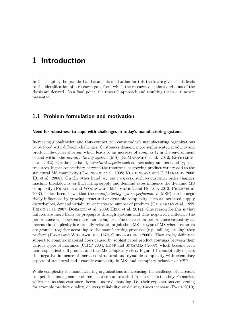
Increasing globalization and thus competition cause today’s manufacturing organizationsto be faced with different challenges. Customers demand more sophisticated products andproduct life-cycles shorten, which leads to an increase of complexity in the environmentof and within the manufacturing system (MS) (ElMaraghy et al. 2012; Efthymiouet al. 2012). On the one hand, structural aspects such as increasing numbers and types ofresources, higher connectivity between the resources, or growing product variety add to thestructural MS complexity (Calinescu et al. 1998; Kuzgunkaya and ElMaraghy 2006;Hu et al. 2008). On the other hand, dynamic aspects, such as customer order changes,machine breakdowns, or fluctuating supply and demand rates influence the dynamic MScomplexity (Frizelle and Woodcock 1995; Vrabič and Butala 2012; Primo et al.2007). It has been shown that the manufacturing system performance (MSP) can be nega-tively influenced by growing structural or dynamic complexity, such as increased supplydisturbances, demand variability, or increased number of products (Guimaraes et al. 1999;Primo et al. 2007; Bozarth et al. 2009; Heim et al. 2014). One reason for this is thatfailures are more likely to propagate through systems and thus negatively influence theperformance when systems are more complex. The decrease in performance caused by anincrease in complexity is especially relevant for job shop MSs, a type of MS where resourcesare grouped together according to the manufacturing processes (e.g., milling, drilling) theyperform (Hayes and Wheelwright 1979; Chryssolouris 2006). They are by definitionsubject to complex material flows caused by sophisticated product routings between theirvarious types of machines (CIRP 2004; Hopp and Spearman 2008), which become evenmore sophisticated if product and thus MS complexity rises. Figure 1.1 conceptually depictsthis negative influence of increased structural and dynamic complexity with exemplaryaspects of structural and dynamic complexity in MSs and exemplary behavior of MSP.
While complexity for manufacturing organizations is increasing, the challenge of increasedcompetition among manufacturers has also lead to a shift from a seller’s to a buyer’s market,which means that customers become more demanding, i.e. their expectations concerningfor example product quality, delivery reliability, or delivery times increase (Patil 2010).
1

1 Introduction
min
ute
s
days
average processing time of an
operation on one machine per day
growing dynamic complexity growing structural complexity
machines
material flow
deteriorating manufacturing system performance
shop calendar day
late
ness
lateness under low
structural and dynamic
complexity
lateness under high
structural and dynamic
complexity
Figure 1.1: Influence of structural and dynamic complexity on manufacturing systemperformance
However, it has been shown that factors such as delivery reliability and delivery timesare largely influenced by the performance of the MS of a company (Sarmiento et al.2007). Delivery dates and thus delivery reliability can for example only be met if thedue dates of production orders in the manufacturing process are met. In order to complywith these increased customer expectations, it is crucial for the success of manufacturingorganizations to keep their MSP at a steady level, although they might be subject togrowing complexity, for example in the form of increased fluctuations. Some companies areeven faced with high contractual penalties if they do not deliver their products on time,for example manufacturers acting as suppliers in the automotive industry (Boysen et al.2015). Moreover, most MSs are part of ever-increasing supply chains in which one tierdepends on the preceding tiers. In such networked systems, it is even more crucial that theperformance of a MSs stays stable in order for delays not to propagate through the entiresupply chain. Incidents where supply chains have been negatively influenced by disruptionshave strongly increased in the past, and so has research on disruption propagation in supplychains (Nair and Vidal 2011; Ivanov et al. 2014; Han and Shin 2015).
Thus maintaining an immutable MSP even in the face of internal and external fluctuationsand disturbances is a desirable characteristic for MSs (Saad and Gindy 1998). This abilityto "maintain specified features when subject to assemblages of perturbations either internalor external" (Jen 2005a) is generally referred to as robustness. The ability of a MS toexhibit an immutable MSP in the face of fluctuations is thus defined as robustness of aMS within this thesis. Robustness in MSs can be measured by analyzing the behavior of a
2

1.1 Problem formulation and motivation
variety of different MSP measures, such as process and product quality (Mondal et al.2014), makespan (Leon et al. 1994), or tardiness (Goren and Sabuncuoglu 2008).
Redundancy as a robustness enabler
With robustness in MSs defined, the question arises which factors influence robustnessin MSs, i.e. how can it be achieved. Resorting to other scientific disciplines, one of themain causes for system robustness in several engineered or biological systems is redun-dancy (Stelling et al. 2004; Kitano 2004; Baker et al. 2008), a term that describes that"several identical, or similar, components (or modules) can replace each other when anothercomponent fails" (Kitano 2004). In a MS context, different resources or capabilities canbe seen as redundancies, for example in job-shop MS machines or raw materials and partsthat can fulfill the same function as others (Levitin and Meizin 2001; Emami-Mehrganiet al. 2011).
However, keeping redundant resources and capabilities in a MS partially contradicts thebasic idea of lean manufacturing principles, which is eliminating waste (i.e. all aspects ofa MS that do not add value to the final product), for example excess inventory or timebuffers (Shah and Ward 2003). Since the 1990’s when lean manufacturing principleswhere introduced to the US-American and European manufacturing domain (Womacket al. 1990), manufacturers have increasingly resorted to them in order to achieve costreduction (Shah and Ward 2003; Bortolotti et al. 2012; Hofer et al. 2012). Yet itwas recently shown that although lean manufacturing principles can lead to cost reduction,they can have a negative influence on MSP (Eroglu and Hofer 2011; Azadegan et al.2013), which in turn can lead to higher costs, for example as a result of missed due dates.Especially if manufacturing complexity rises and fluctuations increase, this has a negativeinfluence on the MSP of extremely streamlined systems which have eliminated all possibleinventories and time buffers (Stecke and Kumar 2009). This has also become evidentrecently when disruptive events such as natural disasters led to production stops in MSs,and consequently to disruptions of entire supply chains (Marsillac and McNamara2013). Moreover, high extra production capacity as a form of redundancy was shownto have a positive effect on plant performance, if the factories are subject to frequentdisruptions and a high level of complexity (Brandon-Jones et al. 2014).
Designing robust manufacturing systems
The existing body of research on robustness in MSs mainly focuses on incorporatingrobustness into MS aspects which require short- to medium-term decisions, for examplerobust production planning and scheduling, robust control, or robust product and processdesign (Nourelfath 2011; Tolio et al. 2011; Mondal et al. 2014). Robust planningand scheduling approaches try to identify robust production plans or schedules, whichthey define as robust if a certain performance measure, such as tardiness or flow time,does not change significantly under unforeseen disturbances (Goren and Sabuncuoglu2010). In robust product and process design, research approaches try to identify and controlthe variables and noise factors that have an influence on the robustness of a product ormanufacturing process, with robustness being achieved if there is minimal variation inend-product quality (Mondal et al. 2014).
3

1 Introduction
MS aspects that require long-term decisions, such as determining the amount of resourcesnecessary for a new MS, are part of manufacturing systems design (MSD) (Chryssolouris2006). Research approaches that incorporate robustness into MSD can be summarizedas robust manufacturing systems design (RMSD) approaches. They define that the designor configuration of a MS is robust if specific performance indicators, such as throughput-times or work in process, do not change significantly when the system is faced withdisturbances (Mezgár et al. 1997; Sharda and Banerjee 2013).
Interdisciplinary methods for robust manufacturing systems design
Research on the topics of robustness and redundancy exists in many different scientificdisciplines. In complex network science, which is the application of graph-theoretical mea-sures to different types of complex natural or man-made networks (Albert and Barabási2002; Newman 2003; Watts 2004; Boccaletti et al. 2006), one of the network charac-teristics that researchers have focused on is robustness (Albert et al. 2000; Callawayet al. 2000; Shargel et al. 2003; Bollobás and Riordan 2004; Beygelzimer et al.2005). Approaches using complex networks measures have been suggested to measure andanalyze (Albert et al. 2000; Callaway et al. 2000) or optimize (Shargel et al. 2003;Beygelzimer et al. 2005) the robustness of different complex networks.
Another scientific discipline where robustness has been studied extensively is in biologicalsystems (Roberts and Tregonning 1980; Wagner 2003; Whitacre 2012). Exemplarysystems where it has been measured and analyzed are food webs (Dunne et al. 2004), plant-pollination networks (Kaiser-Bunbury et al. 2010), metabolic networks (Edwards andPalsson 2000), or cells in general (Stelling et al. 2004). It has been argued that one ofthe main causes for robustness in these biological systems is redundancy (Kitano 2004).The application of graph-theoretic measures to analyze robustness in biological systems iscommon (Jeong et al. 2000), and many of the robustness measures in biological systemsare based on structural aspects of the respective systems (Dunne et al. 2004).
The methods developed in complex network research or biology are able to measure andanalyze the robustness of challenging large-scale, complex systems that are frequently facedwith fluctuations and disturbances. As pointed out in the beginning of this section, theseare the same challenges that MSs are faced with today. Due to these striking similarities,an interdisciplinary transfer of methods that have been developed for solving problems incomplex or biological systems to MSs seems beneficial for manufacturing research.
Research Gap
While numerous approaches in MSD are concerned with incorporating emergent properties,such as flexibility or changeability, into the MS (Tolio 2008; Wiendahl et al. 2007; El-Maraghy 2008), only few approaches are specifically concerned with RMSD. Furthermore,the existing approaches concentrate on creating robust configurations for MSs, but so farno work has focused on identifying factors or conditions that potentially enable or benefitrobustness in MSs. Especially the influence of redundancy on robustness in MSs has notbeen explicitly investigated yet.
4

1.2 Research questions and scope
Methods developed in complex networks science or biology have been successful in theanalysis of robustness in many systems, but their application to MSs is rare. Whileit has recently been shown that complex network measures can be applied to classicalmanufacturing problems, such as machine grouping (Vrabič et al. 2012) or anomalydetection (Vrabič et al. 2013), they have not been applied for MSD or RMSD yet.Moreover, approaches from biology, which were developed to cope with system challengesthat are similar to those in MSs, have neither been applied to analyze robustness in MSs,nor for RMSD.
1.2 Research questions and scope
Guiding research question and sub-questions
As redundancies play an important role for system robustness in other natural or man-madesystems, it is assumed within this thesis that redundancy can also crucially impact therobustness in MSs. Hence the overarching aim of this thesis is to investigate the role ofredundancies as a means to achieve robustness of MSP and to conceptually describe howtointegrate such findings into RMSD. The guiding research question is formed as follows:
Guiding research question. How can redundancies be integrated in manufacturingsystems design so that the manufacturing system performance robustness increases?
This question can be split down in several sub-questions. Firstly, it has to be investigatedwhich definitions and measures of robustness exist in general and in the context of MSs.
Subquestion 1. How can robustness be defined and measured in manufacturing systems?
As a second question, since the term redundancy is not commonly used in a manufacturingcontext, it has to be clarified which definitions and measures of redundancy exist in generaland how they can be conferred to MSs.
Subquestion 2. How can redundancy be defined and measured in manufacturing systems?
After having defined robustness and redundancy in a manufacturing context, it thirdlyhas to be analyzed whether the relationship between robustness of MSP and redundancyis similar to those in other engineered or natural systems, i.e. whether MSP robustnessbenefits from increased redundancy.
Subquestion 3. How is the relationship between robustness of manufacturing systemperformance and redundancy characterized?
Lastly it has to be investigated how measures of robustness and redundancy as well as thefindings about their relationship can be applied in order to design robust MSs.
Subquestion 4. How can redundancy be incorporated in the design and reconfigurationof manufacturing systems in order to increase the robustness of manufacturing systemperformance?
5

1 Introduction
Scope
Within this thesis, the developed models and conducted analysis are limited to job shopMSs, which are systems that usually consist of general-purpose machines that accommodatea large variety of part types. Parts move through the job shop according to their pre-definedprocess plans and route sheets (Chryssolouris 2006), which results in complex routingsof the respective products. Hence job shops are a type of MS that is strongly influenced byincreasing complexity.
MSP, which can consist of a large amount of different performance indicators dependingon the objectives and measurement system of the manufacturing organization (Hon 2005),is narrowed down to a specific MSP indicator within this thesis. The developed modelsand analysis will focus on lateness of production orders, as this indicator is important todraw conclusions regarding the service-level of a manufacturing organization, as presentedin the problem description.
1.3 Research approach and thesis outline
This thesis is divided into seven chapters, which are depicted together with their respectiveresearch methods and objectives in figure 1.2. The first chapter serves as an introduction tothe problem and motivation of the thesis, as well as for presenting the research questions,scope, methods, and outline. The second chapter sets the theoretical background for thethesis, with an introduction to MSs and to existing definitions and measures of robustnessand redundancy. Furthermore, a review of applications of interdisciplinary methods fromcomplex network theory and biology in MSs is given. In the third chapter, measuresfor robustness and redundancy in MSs are developed. Building up on these measures,a model to analyze the relationship between redundancy and robustness is established.The model is analyzed in a discrete-event simulation study, which is a standard methodin MSD and analysis (Negahban and Smith 2014), to investigate whether increasedredundancy is beneficial for robustness of MSP. The fourth chapter suggests a modelingapproach in which nestedness, which is commonly used as an indicator for robustness inecologic systems (Bascompte et al. 2003), is analyzed in a manufacturing context. It isfurther investigated how nestedness is related to robustness of MSP as defined in the thirdchapter. In the fifth chapter, the concept of elementary flux modes (EFMs), which havebeen shown to be a suitable measure to analyze redundancy and robustness in metabolicsystems (Stelling et al. 2002), is transferred to MSs. Similar to the approach in thefourth chapter, the relation of EFMs to robustness of MSP as defined in the third chapteris analyzed here. The sixth chapter describes how the findings on the relationship betweenrobustness and redundancy and the analyzed robustness and redundancy measures can beapplied for designing MSs so that they exhibit a robust system performance. Furthermore, apotential trade-off between robustness, which is induced by redundancy, and cost-efficiencyis discussed. In the last chapter, the results are summarized and implications for industryand further research are presented.
6

1.3 Research approach and thesis outline
Chapter 2
Related Work
Chapter 4
Analyzing nestedness of the part-
resources network of manufacturing
systems
method objective outline
Chapter 5
Analyzing elementary flux modes in
the resources-material flow network
in manufacturing systems
Chapter 6
Designing robust manufacturing
systems with redundancy
considerations
modeling
elementary
flux mode
analysis
modeling
nestedness
analysis
literature
review
modeling
discrete-event
simulation
Chapter 3
Analyzing the relationship between
robustness and redundancy in
manufacturing systems
give definitions and measures for robustness
and redundancy
measure robustness and redundancy in
manufacturing systems
analyze relationship between robustness and
redundancy
measure nestedness in manufacturing
systems
analyze relationship between robustness and
nestedness
measure elementary flux modes in
manufacturing systems
analyze relationship between robustness and
elementary flux modes
explain how the analyzed measures can be
applied for robust manufacturing system
design
Chapter 1
Introduction
present problem, motivation, research
questions and approach
Chapter 7
Conclusion
summarize results, explain contribution to
academia & industrial practice, give outlook on
further research and application
Figure 1.2: Thesis outline, research methods, and objectives
7

2 Related Work
This chapter gives an introduction to aspects and topics that are relevant within the scopeof this thesis. In the beginning, the underlying understanding of MSs, their objectives andperformance measures, as well as current challenges are introduced. This is followed byan overview on MSD in section 2.1, with a more detailed presentation of specific designmethods for job shop MSs, as they are the focus of this thesis. Definitions and measuresof robustness and redundancy are reviewed in section 2.2, first in general and then witha specific relation to MSs. Since many of the reviewed definitions of robustness andredundancy are from the context of other scientific areas, the background on the otherrelevant disciplines, such as complex network science and biology, and the benefits ofinterdisciplinary transfer between these disciplines are given in section 2.3. As a last step,the research gap is derived from the presented works in section 2.4.
2.1 Introduction to manufacturing systems
2.1.1 Definition and terms of manufacturing systems
In order to answer the guiding research question of this thesis how redundancies can beintegrated in MSD to create RMSP, this section first establishes the general definition of aMS. The term production in a general sense refers to "the process of creating goods and/orservices" (Bellgran and Säfsten 2009) or "creating something new" (Hitomi 1996),which includes tangible goods such as tools, cars, electronics, or intangible goods such asconsulting services, music, or energy production (Hitomi 1996; Bellgran and Säfsten2009). The term manufacturing is used in a narrower sense, as the "production of tangiblegoods" (Hitomi 1996), but also comprises "the entirety of interrelated economic, technologi-cal, and organizational measures directly connected with the process/machining of materials,i.e. all functions and activities directly contributing to the making of goods" (Segreto andTeti 2014). The functions and activities mentioned in the former definition are specifiedby some authors to be planning, design, procurement, manufacturing production, inventory,marketing, distribution, sales, quality assurance, marketing, and management (CIRP 2004;Hitomi 1996).
A broad range of definitions in standard textbooks, papers, and encyclopedias also existsfor the term MS (Black 1991; Wu 1994; Hitomi 1996; Suh et al. 1998; Chryssolouris2006; DeGarmo et al. 2011; Caggiano 2014). Some authors focus on the tasks andprocesses of manufacturing (Wu 1994; Hitomi 1996), defining a MS as a system employing"a series of value-adding manufacturing processes to convert the raw materials into moreuseful forms and eventually into finished products" (Wu 1994). Others put an emphasison the most important physical elements (Black 1991; Suh et al. 1998; Chryssolouris
8

2.1 Introduction to manufacturing systems
2006; DeGarmo et al. 2011; Caggiano 2014) and define a MS as "a combination ofhumans, machinery and equipment that are bound by a common material and informationflow" (Caggiano 2014). It is important to note here that while some authors see theterm production system defined as a subsystem of a MS (Bellgran and Säfsten 2009),within this thesis the two terms are considered to be synonymous as suggested by severalother authors (Hitomi 1996; Caggiano 2014).
When defining the term MS, several authors stress that these systems can be depicted andperceived according to a systems theoretic approach (Wu 1994; Hitomi 1996; Papadopou-los et al. 2009; Bellgran and Säfsten 2009). Systems theory is a transdisciplinaryresearch field which is based on the idea that different systems from all kinds of scien-tific fields share common characteristics. A system’s characteristics are, for example,to transform inputs into outputs, to consist of elements which are connected and haveinterrelations, to exhibit emergent properties, and to have an objective or purpose (Check-land 1999; Bertalanffy 2003; Meadows 2009). Emergent properties are propertiesthat a system exhibits as a whole, but that none of its elements exhibit separately, whichis often referred to as the whole is more then its single parts (Skyttner 2005). Suchproperties are of special interest to many research approaches on MSs, and researchers havefocused on incorporating different emergent system properties such as flexibility (Sethiand Sethi 1990; Tolio 2008), agility (Kidd 1994; Yusuf et al. 1999; Sanchez andNagi 2001), reconfigurability (Koren et al. 1999; Dashchenko 2007; ElMaraghy2008), changeability (Wiendahl et al. 2007; ElMaraghy 2008) or robustness (Windt2012; Mondal et al. 2014) into MSs. Within this thesis, a MSs is defined as suggestedby DeGarmo et al. (2011), as a "complex arrangement of physical elements characterizedby measurable parameters" (DeGarmo et al. 2011), which stresses the system theoreticaspects of a MS. Figure 2.1 gives an example of a MS with its inputs, outputs, and elements.Possible inputs such as materials, energy, etc, are depicted on the left, possible outputs suchas products, information, defectives etc. are shown on the right side. Machines, tooling, orworkers are listed as examples for physical elements in the middle.
manufacturing system materials
energy
demand
information
good products, parts etc.
defectives, scrap
sub-assemblies
from design,
purchasing, production
control, etc.
a complex arrangement of physical
elements such as
machines for processing
tooling (fixtures, dies, cutting
tools)
materials handling equipment
(which includes all transportation
and storage)
people (operators, workers,
associates)
information
service to customer
Figure 2.1: Definition of a manufacturing system with its inputs and outputs, modifiedfrom (DeGarmo et al. 2011)
Some of the inputs and outputs in MSs are physical, such as machines, manual workstations,material handling or tooling equipment, human workforce, raw material, purchased parts,
9

2 Related Work
manufactured products, or defectives (Hitomi 1996; Chryssolouris 2006; Caggiano2014). In addition to these physically tangible aspects, there is a large amount of differ-ent informational inputs and outputs that are needed to operate the MS. The quantities andtypes of raw materials, sub-assemblies, or purchased parts that are needed to manufacturea product are listed in the bill of material (BOM) of a product (DeGarmo et al. 2011). ABOM can have different formats, for example just a simple list or a product-structure graph.The sequence of different manufacturing processes that are necessary to transform the ma-terials into the final product are denoted in the process plan of a product (Scallan 2003).The operations, which are the activities in which the materials are changed (Heragu 2006),are a more detailed version of the manufacturing processes denoted in the process plan. Ifdrilling is the general manufacturing process a part has to undergo, the operation specifiesthe necessary parameters to carry out this process, such as required resources (machines,tools), or processing times. The operations sheet or route sheet of a product then lists theoperations necessary to manufacture the entire product in the correct sequence, includinginformation such as resources, processing times on the resources, or set-up times on theresources (Heragu 2006; DeGarmo et al. 2011). This specifies a product’s route, which isdefined as "the set of work centers or machines through which a product is processed" (Dasand Nagendra 1997). If different resources are able to fulfill the same manufacturingprocess and thus operation, products can take different, alternative routes through theMS. A production order is what triggers the production of a product in the productiondepartment and contains information on the product quantity to manufacture, due dates,the necessary operations, material components and production resources (CIRP 2004).The term job can refer to a series of processing steps necessary to create a product (similarto the production order) (Curry and Feldman 2010), but more commonly, it refers tothe working duties and physical materials to be performed on one particular work station(similar to the operation). In the latter case, the relation between jobs and orders is notone-to-one, but an order for a product consists of several jobs (Hopp and Spearman 2008;DeGarmo et al. 2011).
As stated in the introductory chapter, the focus of this thesis is on job shop MSs, and inparticular on the design of such systems, as they are by definition subject to complexity (e.g.complex routings (CIRP 2004)) and thus are prone to a negative influence by increasingcomplexity (e.g. increased fluctuations). In order to be able to properly distinguish ap-proaches for MSD of job shop MSs from design approaches for other MSs, an overview on thedifferent types of MSs is given in the following. Depending on the product types and volumesthat are to be manufactured, five general types of MSs can be distinguished: the projectshop, the job shop, the cellular shop, the flow shop, and continuous systems (Hayes andWheelwright 1979; Wu 1994; Suh et al. 1998; Chryssolouris 2006; Heragu 2006;DeGarmo et al. 2011; Caggiano 2014). Figure 2.2 gives a conceptual depiction of four ofthese five different types. In a project shop or fixed-site production, the product has a fixedposition and the resources such as materials and machines are brought to the product asneeded (see figure 2.2a). This is usually because of the size and/ or weight of the products,which typically are aircrafts, ships, or large structures such as bridges (Chryssolouris2006). In job shops, resources are grouped together according to the manufacturing pro-cesses (e.g., milling, drilling) they perform (see figure 2.2b). The products move throughthese machines according to the processes that are denoted in their process plans, so thatcomplex material flows can arise (CIRP 2004). In cellular shops or group productionsystems, machines are not grouped according to similar manufacturing processes, butaccording to product families that require similar manufacturing processes (see figure 2.2c).
10

2.1 Introduction to manufacturing systems
Thus the material flow induced by a certain product concentrates on the resource centerthat is responsible for this product (Chryssolouris 2006). In flow shops, which are alsoreferred to as flow lines, resources are ordered in lines in the specific process sequence ofa product, where each product has its own line of resources (see figure 2.2d). A specialtype of flow shops are transfer lines, also known as paced lines, which are flow lines with asynchronous movement of material flow between the different resources. They are typicallyfound in automotive production (Papadopoulos et al. 2009). The fifth type of MS isthe continuous system (not depicted in the figure). Contrary to the previously introducedMSs which all produce discrete parts, a continuous system treats liquid materials, such asfluids, gases, or powder and is thus arranged in a special type of flow line (Papadopouloset al. 2009).
raw material
A
A
ready part
B
B
C D
D
D
(a) project shop
raw material
B B
B B
ready part
A A
A A
A A
C C
C C
C C
(b) job shop
raw material
ready part
B C
D E
A B
D F
D E
F G
(c) cellular-shop
raw material
A
A
ready part
G
C
D
B
D
F
F
B
F
(d) flow-shop
Figure 2.2: Exemplary types of manufacturing systems, modified from (Chryssolouris2006)
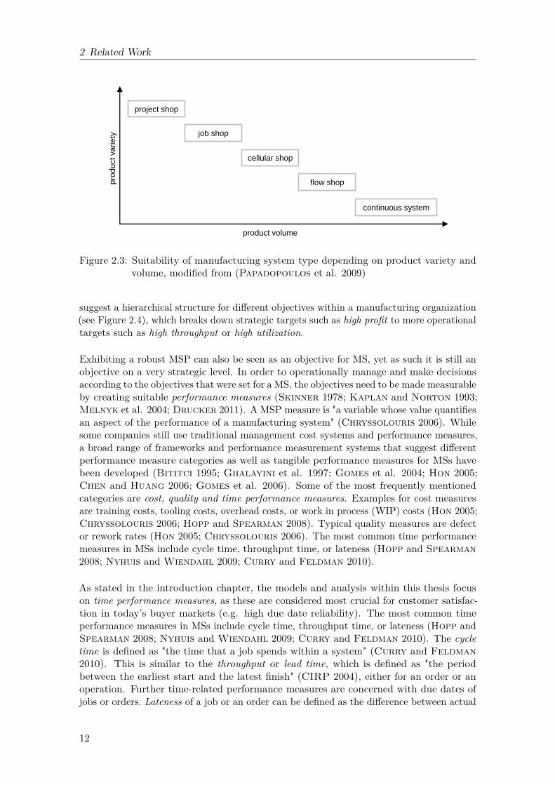
MSs implemented in the real world usually are a combination of these standard archetypesof MSs, or exhibit slight alterations to these standards. An example for such a hybrid typeof MS is the flexible manufacturing system (FMS), which is a combination of a job shopand a cellular shop (Chryssolouris 2006). The choice of a type of MS strongly dependson the characteristics of the product to be manufactured, such as variety, lot sizes, orvolumes (Papadopoulos et al. 2009). In figure 2.3, the five types of MSs are positionedaccording to the product variety and volumes for which they are mostly used.
2.1.2 Objectives, trade-offs, and performance in manufacturing systems
As this thesis strives to answer the question of how RMSP can be achieved by integratingredundancy, the general objectives and trade-offs in MSs, as well as a definition of perfor-mance and important performance indicators in MSs have to presented. In general, theobjectives of a MS depend on the product types and volumes to be produced in the MS.Although the fundamental objective of a manufacturing organization in general usuallyis to make profit and to ensure the existence of the organization (Hitomi 1996; Hoppand Spearman 2008), such strategic objectives like profit or customer-orientation are notsuitable for operational decisions within the MS. Therefore the strategic objectives of acompany need to be broken down to a more operational level, which allows assessing theperformance of sub-systems such as the MS. To achieve this, Hopp and Spearman (2008)
11
2 Related Work
product volume
project shop
job shop
cellular shop
flow shop pro
duct variety
continuous system
Figure 2.3: Suitability of manufacturing system type depending on product variety andvolume, modified from (Papadopoulos et al. 2009)
suggest a hierarchical structure for different objectives within a manufacturing organization(see Figure 2.4), which breaks down strategic targets such as high profit to more operationaltargets such as high throughput or high utilization.
Exhibiting a robust MSP can also be seen as an objective for MS, yet as such it is still anobjective on a very strategic level. In order to operationally manage and make decisionsaccording to the objectives that were set for a MS, the objectives need to be made measurableby creating suitable performance measures (Skinner 1978; Kaplan and Norton 1993;Melnyk et al. 2004; Drucker 2011). A MSP measure is "a variable whose value quantifiesan aspect of the performance of a manufacturing system" (Chryssolouris 2006). Whilesome companies still use traditional management cost systems and performance measures,a broad range of frameworks and performance measurement systems that suggest differentperformance measure categories as well as tangible performance measures for MSs havebeen developed (Bititci 1995; Ghalayini et al. 1997; Gomes et al. 2004; Hon 2005;Chen and Huang 2006; Gomes et al. 2006). Some of the most frequently mentionedcategories are cost, quality and time performance measures. Examples for cost measuresare training costs, tooling costs, overhead costs, or work in process (WIP) costs (Hon 2005;Chryssolouris 2006; Hopp and Spearman 2008). Typical quality measures are defector rework rates (Hon 2005; Chryssolouris 2006). The most common time performancemeasures in MSs include cycle time, throughput time, or lateness (Hopp and Spearman2008; Nyhuis and Wiendahl 2009; Curry and Feldman 2010).
As stated in the introduction chapter, the models and analysis within this thesis focuson time performance measures, as these are considered most crucial for customer satisfac-tion in today’s buyer markets (e.g. high due date reliability). The most common timeperformance measures in MSs include cycle time, throughput time, or lateness (Hopp andSpearman 2008; Nyhuis and Wiendahl 2009; Curry and Feldman 2010). The cycletime is defined as "the time that a job spends within a system" (Curry and Feldman2010). This is similar to the throughput or lead time, which is defined as "the periodbetween the earliest start and the latest finish" (CIRP 2004), either for an order or anoperation. Further time-related performance measures are concerned with due dates ofjobs or orders. Lateness of a job or an order can be defined as the difference between actual
12

2.1 Introduction to manufacturing systems
high
ROI
low assets high
profit
low costs high sales high
utilization low inventory
less variability high customer
service low price low unit costs
high
throughput
high
utilization low inventory fast response
many
products
more
variability high inventory low utilization
short cycle
times less variability
quality
product
Figure 2.4: Hierarchical objectives in a manufacturing organization, modified from (Hoppand Spearman 2008)
completion time and planned completion time (due date) (Nyhuis and Wiendahl 2009;Pinedo 2012; Framinan et al. 2014). A measure similar to lateness is tardiness of ajob, which is defined as the lateness of the job in case it is negative and zero for all jobswith positive lateness (Hopp and Spearman 2008; Pinedo 2012; Framinan et al. 2014).In the same manner, earliness of a job is defined as the lateness of the job in case it ispositive and zero for all jobs with negative lateness. The percentage of tardy or early jobs isoften used to assess schedule reliability of a production schedule (Pinedo 2012; Framinanet al. 2014) or to measure the due date performance towards the customer (Hopp andSpearman 2008).
In the hierarchical structure of objectives as shown in Figure 2.4, some of the objectives,such as high utilization which is shown as a sub-objective of low unit costs, are the oppositeof other objectives, such as low utilization which is shown as a sub-objective of fastresponse. Such trade-offs between different objectives in MS are common and in orderto resolve them, the manufacturing organization has to choose a position, since not allobjectives can be reached at the same time (Skinner 1969; Hayes and Wheelwright1984; Mapes et al. 1997; Da Silveira and Slack 2001; Da Silveira 2005). A depictionof objectives for MSs that focuses on these trade-offs is the manufacturing tetrahedronsuggested by (Chryssolouris 2006). The authors claim that every decision in a MS shouldbe taken considering the objectives time, quality, costs, and flexibility. The representation ina tetrahedral form (see Figure 2.5) emphasizes the trade-off, i.e. that not all four objectivescan be optimized simultaneously. A further definition of MS objectives and their trade-offsis given in the manufacturing planning dilemma (Gutenberg 1983; Wiendahl 2014). Itdescribes the two benefit objectives high due date reliability and short throughput-timeson the one hand, and the two cost objectives high utilization and low inventory on the
13

2 Related Work
cost
time flexibility
quality
Figure 2.5: The manufacturing tetrahedron (Chryssolouris 2006)
other hand (see Figure 2.6). These objectives stand in a trade-off relationship: customerswould like to receive their goods at the promised time (high due date reliability) and assoon as possible after they ordered them (short throughput time), companies howeverwould like to keep their utilized machine capacity at a steady level to avoid idle time costs(high utilization) and their spare parts and finished goods inventory low in order to saveinventory carrying costs (low inventory). The performance and cost objectives are thereforealso referred to as the customer view and the company view (Wiendahl 2014).
high benefits
customer-view
company-view
low costs
low throughput-time high due-date reliability
high utilization low inventory
profitability
Figure 2.6: The manufacturing control dilemma, modified from (Wiendahl 2014)
Such trade-offs could potentially also exist between robust MSP and other objectives in MSs.If robustness of MSP was for example achieved by increasing inventory or excess resources,this would stand in a trade-off to the objective of low inventory costs or low investmentcosts, which can be summarized as cost-efficiency. A trade-off between robustness andefficiency is for example also described for supply chains by Shukla et al. (2011). Whenit is the objective to design a MS in a way that its performance stays robust in the face offluctuations and disturbances, the trade-off between robust MSP and cost-efficiency has tobe taken into account.
14

2.1 Introduction to manufacturing systems
2.1.3 Manufacturing systems design
Different sub-tasks of manufacturing systems design
Since the guiding research question of this thesis focuses on how robustness can be achievedby integrating redundancy in MSD, an introduction to the different sub-tasks in MSD isgiven here. Moreover, existing methods and approaches for the design of job shop MSsare reviewed in the next section. Once the objectives and performance requirements ofa manufacturing organization have been set (i.e. which products to produce, at whichcustomer service level), a suitable MS to fulfill these requirements has to be designed (Suhet al. 1998; Chryssolouris 2006). As presented in section 2.1.1, MSs consist of a largeamount of different elements (e.g., machines, tooling) and the relations between them (e.g.,control procedures for the interaction of elements). Decisions concerning the elementsand the relations between them, such as the material processing structure (e.g., the typeof manufacturing processes and structure needed to produce the desired products), theresource quantities (e.g., amount of machines, workforce), or the resource layout, aretaken in MSD phase (Chryssolouris 2006; Heragu 2006; Schenk et al. 2009). Thesedesign decisions usually have a long-term effect (years) on the MS, as the amount ofmachines and also the general layout are not frequently changed. This is also sometimesreferred to as steady state design, whereas decisions such as sizing of buffer inventories,setting of stock order policies, or workforce capacity adjustment are termed dynamicdesign (Parnaby 1979). Figure 2.7 compares the long-term decisions taken in MSD tomid-term and short-term decisions. Tasks such as production planning, master scheduling,material requirements planning, or capacity planning are considered to involve decisions ona medium-term time horizon (weeks to months), while tasks such as scheduling, dispatching,or shop floor control implicate short-term decisions (hours to days) (Bahl and Ritzman1987; Altiok 1997; Hopp and Spearman 2008; Pinedo 2012). While some authors alsoconsider medium-term and short-term decisions on the planning and control of MSs to bepart of MSD (Davis et al. 1986; Papadopoulos et al. 1993; Cochran et al. 2001), onlythe setting of long-term, structural aspects of the MS is considered as MSD within thisthesis. MSD often is a complex task and is thus usually decomposed into sub-problems,which are treated hierarchically and sometimes in several iterative loops (Chryssolouris2006; Heragu 2006; Timm and Blecken 2011).
long-term medium-term short-term
manufacturing system
design
manufacturing system
planning manufacturing system
control
design of process
structure, equipment
quantities, equipment
layout
production planning,
master scheduling,
material requirements
planning, capacity
planning
scheduling, dispatching,
shop floor management tas
ks
Figure 2.7: Decision horizons in manufacturing systems, modified from (Papadopouloset al. 1993; Hopp and Spearman 2008; Pinedo 2012)
15

2 Related Work
MSD starts after the product structure has been established. As depicted in figure 2.8,the product design determines which manufacturing processes - and consequently whichtypes of resources - are necessary to produce the final products, which is done in the phaseof process planning (Scallan 2003). This also influences how the BOMs and route sheetsof products will look like. Depending on the estimated volumes and different manufacturingprocesses required to manufacture the desired products (derived from the process plans ofthe products (Scallan 2003)), the necessary quantities of the manufacturing resources(e.g., machines, tools, workforce) can then be calculated.
manufacturing systems are
designed according to the products
to be manufactured
in a first step, products are
designed
information about the products
is used to create a process
plan in which the necessary
manufacturing processes are
described
according to the process plan,
manufacturing engineers
select the necessary
resources (machines, tools)
for manufacturing the products
[cf. Scallan 2003, Chryssolouris 2006]
0
1 3
1.1 1.2
2
3.1 3.2
product
sub-assembly
raw material
product design process planning resource design
exemplary product structure
1.1
1.2
raw material/ part operations
drilling
milling
welding
operation resource
drilling
welding
A
B
D
drilling
milling C
exemplary process plan exemplary resource list
determination of product
types & variety
structure
materials
determination of
manufacturing operations
types
tools
determination of resource
types
amount
Figure 2.8: Relation between product design and resource design
The phase termed resource design in figure 2.8 is also referred to as the resource requirementsproblem (Chryssolouris 2006), dimensioning (Schenk et al. 2009), or sizing (Roze andKasilingam 1996; Masmoudi 2006) of MSs. Sub-problems within the resource require-ments problem are concerned with determining machine requirements (Miller and Davis1977; Hayes et al. 1981; Jain et al. 1991) or production equipment requirements (Kusiak1987; Bard and Feo 1991). After the resource requirements have been determined, afurther part of MSD is resource layout design, which describes the problem of optimizingthe physical arrangement of the resources within the constrained available space of themanufacturing facility (Rosenblatt 1979; Kusiak and Heragu 1987; Benjaafar et al.2002; Singh and Sharma 2006).
Most approaches for MSD are tailored to the characteristics and requirements of one ofthe different types of MSs introduced in section 2.1.1 and are thus not interchangeablyapplicable. An example for this are approaches for the design of cellular shops, in which itis often first determined which resources should be grouped together in cells and then whichdimension (i.e. number of resources) the cells should have (Opitz and Wiendahl 1971;Rajagopalan andBatra 1975; Askin 2013). Another example are design approaches thatare specifically tailored for production lines, which for example do not exhibit alternativeroutes like job shops, as the manufacturing processes are ordered sequentially (Nahaset al. 2009). In addition to that, approaches to determine the resource requirementsand resource layout of MSs in the design phase have to be clearly distinguished fromapproaches for capacity planning, capacity management, or capacity expansion in MSs.The term capacity in a manufacturing context refers to the general ability of a MS toproduce a certain output per time period or to perform its expected function (CIRP 2004;Crowson 2005), the more specific machine capacity for example refers to the capability of
16

2.1 Introduction to manufacturing systems
a single machine to produce output per time period (Crowson 2005). While decisionson resource requirements and resource layout during MSD are taken to create the entireMS, capacity management or expansion decisions are taken on a tactical to operationaldecision horizon to decide whether capacity investments are necessary in order to meet theupcoming demand of a specified time horizon (Matta et al. 2005; Chryssolouris 2006;Ceryan and Koren 2009). Although some authors consider capacity planning to be thedetermination of the long-range production capacity in the facility (Askin and Mitwasi1992), the term resource requirements is used within this thesis.
Determining resource requirements in job shop manufacturing systems
As mentioned in the previous section, approaches for MSD are usually tailored to one of theintroduced types of MSs. Since this thesis focuses on job shop MSs, this section presentsdifferent modeling approaches that can be applied to job shop MSs. The focus here lies onthe presentation of modeling approaches to determine the resource requirements in jobshop MS, which was introduced as one of the sub-tasks in MSD in the previous section(see 2.1.3). Modeling approaches to determine resource requirements in other MS types,such as cellular systems or transfer lines, are not covered here, for they substantially differfrom approaches for MSD of job shop MS. In cellular shops for example, the groupingand layout of resources needs to be solved simultaneously to the problem of resourcedimensioning, which requires different input and output parameters than the design of jobshop MSs.
The parameters that need to be determined when the resource requirements of a jobshop have to be set are the different types and amounts of necessary resources, such asmachines, tools, handling, or transport equipment. The resource requirements depend on alarge amount of different influencing factors, for example the products to be manufactured,the demand and its potential fluctuations, or the technological abilities of the resources. Anearly review paper by Miller and Davis (1977) gives a detailed overview on existing simpleanalytical models to solve the machine requirements problem in job shop MS, of which anexcerpt is shown in table 2.1. The first model in the table is the most general one anddetermines the amount of resources necessary for a single period and a single machine case,and thus has a very limited system scope. The influencing variables considered by thismodel are operation times, number of products required, machine capacity, and efficiency.The second model in table 2.1 does take into account multiple machines, but still does notdetermine the amounts of machines necessary for multiple periods. A more sophisticatedmodel is the third model presented in table 2.1, which recognizes the stochastic nature ofthe variables under study (such as the production demand) by including distributions forthem.
Miller and Davis (1977) conclude that the simple models so far did not take into accountfactors that have a significant influence on the number of machines necessary, such as costrestrictions or fluctuations in input variables like the demand. Therefore they suggesta linear programming and a mixed integer programming model to find the optimal numberof machines under cost constraints and varying demands in a serial, multistage MS (Davisand Miller 1978; Miller and Davis 1978). These early mathematical optimizationmodels have gradually been enhanced, for example by Hayes et al. (1981), who suggesta dynamic programming model for finding the cost-minimal solution to the machine
17

2 Related Work
Formula Variables
x = ( t60 )( p
hu )
x = required number of machinest = standard time for operation in minutesp= total number of production units required per dayh= standard number of hours available per day per machineu= efficiency of the machine (as a percentage)
xj =n∑
i=1
pi j ti jhi j
xj = required number of machines of type jpi j = desired production rate for product i on machine jti j = standard production time for product i on machine jhi j = number of hours available for product i on machine jj = machine typei = product type
x =∑
i
∑j
ti j pihu ,
x = g(h1(ti j ), h2(pi ), h3(u))
x = required number of machinesti j = performance time for operation j on product ipi = production demand per period for product ih = standard hours available per periodu = effectiveness factorj = operationi = producth1(ti j ) = distribution of the performance timeh2(pi ) = distribution of the production demandh3(u) = distribution of the effectiveness factorg(.) = joint probability function
Table 2.1: Calculation approaches to solve the machine requirements problem, modifiedfrom Miller and Davis (1977)
requirements problem. A further model introduces two simplified linear programmingmodels to determine the cost-minimal amount of machines and handling equipment, arguingthat the existing models are too specific in their data requirements to be suitable forapplication in industrial practice (Kusiak 1987). The linear programming model of Bardand Feo (1991) offers an even more generalized mathematical formulation of the machinerequirements problem, yet it is the first one to account for process flexibility, thus makingit more suitable for job shop MSs. Further authors then proposed different formulations toaddress the machine requirements problem in integer programming models that considerprocess flexibility (Roze and Kasilingam 1996; Kasilingam and Roze 1996). Mak andWong (1999) also developed a mathematical model of the machine requirements planningproblem and develop a solution technique based on a genetic algorithm.
The general inputs to the mathematical optimization models are similar among the differentmodels. Apart from cost data on operational and fixed costs of the resources, mathematicalprogramming approaches need as inputs for their models information on the types ofproducts to be manufactured and their demands, the manufacturing processes required tocreate the products, a list of available machine types, and the operation times or efficienciesfor the processes on the different machines (Miller and Davis 1978; Bard and Feo 1991;Roze and Kasilingam 1996). An example for model input data for a problem with 4products, 6 processes, and 5 machines which was presented by Bard and Feo (1991) isshown in table 2.2. Table 2.2a shows which different manufacturing processes a productneeds and the time it needs for the respective process. It furthermore gives the demand forthe products in a certain time-period. Table 2.2b shows the manufacturing processes, on
18

2.1 Introduction to manufacturing systems
which machines they can be carried out and the efficiencies of the different machines forthe respective process. It also depicts the discounted costs per machine.
productprocess 1 2 3 41 3.2 0.0 14.3 12.32 8.5 0.0 10.2 0.33 1.5 5.3 0.0 2.54 4.5 0.0 3.2 0.15 0.5 1.1 2.2 0.06 0.0 5.1 0.2 4.3demand 0.92 0.54 0.76 0.79
(a) Product-process data
machineprocess 1 2 3 4 51 4.7 1.9 0.0 0.0 0.12 5.2 4.4 3.7 2.0 0.03 0.2 3.0 4.9 7.0 0.04 0.0 0.0 2.0 5.3 1.45 0.0 0.0 0.0 1.6 7.16 0.0 0.6 0.0 0.3 3.0cost 249.5 184.7 138.3 221.3 232.8
(b) Process-machine data
Table 2.2: Input data to determine machine requirements, modified from (Bard and Feo1991)
Researchers have also resorted to modeling job shop MSs as queues or networks of queues inorder to determine the necessary amount of resources required for a job shop MS (Bitranand Dasu 1992; Buzacott and Shanthikumar 1992; Papadopoulos et al. 1993).A queuing process usually consists of customers that arrive at a service facility, wherethey wait in a line (queue) if all servers are busy, until they receive service from a sever,and then depart from the facility. A queuing model is usually constructed to predict thequeue lengths and waiting times of customers in a system (Gross et al. 2008). It canbe described by six characteristics, which are the arrival pattern of the customers, theservice patterns of the servers, the queue discipline, the system capacity, the number ofservice channels, and the number of service stages (Gross et al. 2008). In the case ofMSs, the servers correspond to the resources in a MS, while the customers correspond tomanufacturing orders or jobs (Papadopoulos et al. 1993; Chryssolouris 2006). Tomodel an entire job shop MS with several resources, the resources are regarded as a networkof single server queues, for which performance measures are individually recorded and thenaveraged for the overall MS (Bitran and Tirupati 1989a; Bitran and Morabito 1999;Govil and Fu 1999). As Bitran and Morabito (1999) describe, queuing approachescan be distinguished into those whose objective it is to minimize the investment in the MSsubject to MS performance constraints, or those whose objective it is to maximize the MSperformance subject to a limited budget for investment in the MS.
Another method used to solve the resource requirements problem is simulation model-ing (Law and McComas 1998), which was suggested as early as the first mathematicaloptimization approaches (Reasor et al. 1977). In Reasor et al. (1977), the numberof machines is determined under the assumptions that total costs should be minimizedand a given target production quantity should be reached. Their model serves as anexperimental tool to evaluate different system configurations, as it allows for changingsystem characteristics such as machine operating rates or the scheduling logic. More recentapproaches do not only focus on cost optimization as early approaches of mathemati-cal optimization, but also consider achieving a certain level of MSP with their systemdesigns. Feyzioğlu et al. (2005) use a simulation model combined with a boot strapapproach to identify the minimum number of machines necessary to fulfill certain definedmanufacturing performance goals. In a similar approach, a simulation model is coupledwith an expert system to find the amount of resources where tardiness is minimized asa primary objective while earliness is minimized as a secondary objective (Masmoudi
19
2 Related Work
2006). To sum it up, the methods used in approaches for machine requirements design forjob shop MSs are traditional (deterministic), mathematical programming, queuing based,or simulation approaches (Chryssolouris 2006; Heragu 2006; Negahban and Smith2014).
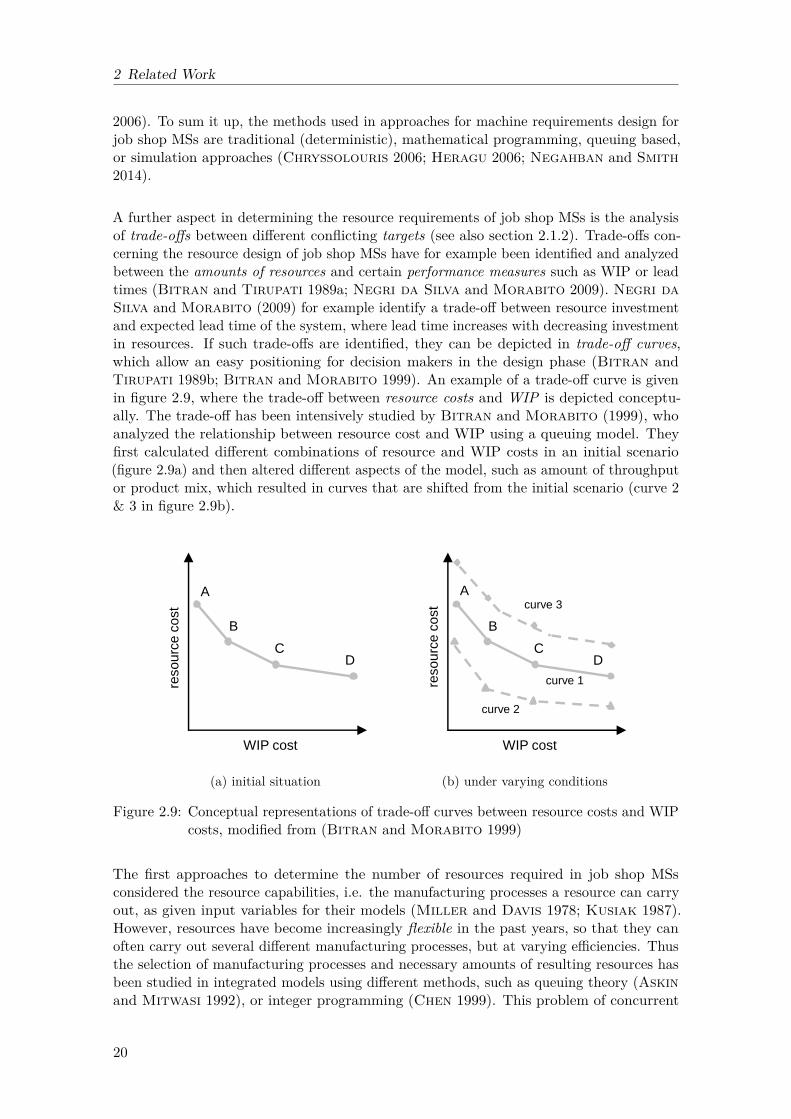
A further aspect in determining the resource requirements of job shop MSs is the analysisof trade-offs between different conflicting targets (see also section 2.1.2). Trade-offs con-cerning the resource design of job shop MSs have for example been identified and analyzedbetween the amounts of resources and certain performance measures such as WIP or leadtimes (Bitran and Tirupati 1989a; Negri da Silva and Morabito 2009). Negri daSilva and Morabito (2009) for example identify a trade-off between resource investmentand expected lead time of the system, where lead time increases with decreasing investmentin resources. If such trade-offs are identified, they can be depicted in trade-off curves,which allow an easy positioning for decision makers in the design phase (Bitran andTirupati 1989b; Bitran and Morabito 1999). An example of a trade-off curve is givenin figure 2.9, where the trade-off between resource costs and WIP is depicted conceptu-ally. The trade-off has been intensively studied by Bitran and Morabito (1999), whoanalyzed the relationship between resource cost and WIP using a queuing model. Theyfirst calculated different combinations of resource and WIP costs in an initial scenario(figure 2.9a) and then altered different aspects of the model, such as amount of throughputor product mix, which resulted in curves that are shifted from the initial scenario (curve 2& 3 in figure 2.9b).
WIP cost
reso
urc
e c
ost
A
B
C D
(a) initial situation
WIP cost
resourc
e c
ost
A
B
C D
curve 1
curve 2
curve 3
(b) under varying conditions
Figure 2.9: Conceptual representations of trade-off curves between resource costs and WIPcosts, modified from (Bitran and Morabito 1999)
The first approaches to determine the number of resources required in job shop MSsconsidered the resource capabilities, i.e. the manufacturing processes a resource can carryout, as given input variables for their models (Miller and Davis 1978; Kusiak 1987).However, resources have become increasingly flexible in the past years, so that they canoften carry out several different manufacturing processes, but at varying efficiencies. Thusthe selection of manufacturing processes and necessary amounts of resulting resources hasbeen studied in integrated models using different methods, such as queuing theory (Askinand Mitwasi 1992), or integer programming (Chen 1999). This problem of concurrent
20
2.1 Introduction to manufacturing systems
selection of manufacturing processes and equipment selection is still a focus of currentresearch (Kulak et al. 2005; Dagdeviren 2008).
A further issue in the design of job jop MSs is the development of decision support systemsto aid in the design phase of MSs. Such approaches use mathematical programming orsimulation as an underlying method, but focus on designing user-friendly software systemsto present the modeling results in order to facilitate design decisions (Gopalakrishnanet al. 2004; Chtourou et al. 2005; Guldogan 2011; Longo et al. 2012). Longo et al.(2012) for example develop a decision support system, which is based on a discrete-eventsimulation model, to aid deciding on a plant design during the MSD phase. In their model,industrial plant parameters (such as machine capacity, the arrival time and amount of rawmaterial, the number of workers per department, and the product mix) can be varied andtheir influence on plant production and performance can be analyzed.
2.1.4 Negative influence of complexity and disturbances on manufacturingsystem performance
The MSP (as introduced in section 2.1.2) can be influenced by a multitude of differentfactors, and thus does not constantly stay the same in real life MSs. Even if a job shopMS was designed by considering a certain amount of fluctuations in the input parameters(see section 2.1.3), MS are still prone to uncertainty and unforeseen events. A perturbation,which in a general meaning is "a deviation of a system, moving object, or process fromits regular or normal state or path" (Stevenson 2010), is in the manufacturing contextreferred to as a disturbance or disruption, which is an unplanned or unpredictable event inthe state or function of the MS (Kuivanen 1996; Saad and Gindy 1998; Frizelle et al.1998; Ingemansson and Bolmsjö 2004). In recent years, manufacturing organizationshave been increasingly faced with disturbances. A survey among 151 large U.S. companiesshowed that 73% of the organizations had experienced disturbances (Accenture 2008),and several recent studies point out that disturbances are expected to occur even morefrequently in the future (Cook 2008; Bhatia et al. 2013; Deloitte 2015).
Different reviews and classification schemes of disturbances exist in MS research (Farhoodi1990; Frizelle et al. 1998; Saad and Gindy 1998). Farhoodi (1990) classify disturbancesin MSs according to the source of origination of the disturbance, e.g. order related distur-bances such as early or late orders, and resource related disturbances such as machine ortransport breakdowns. In Frizelle et al. (1998), a classification of disturbances accordingto when they occur with regard to the manufacturing process is offered. They distinguishbetween upstream, internal, or downstream disturbances and give examples for all threecategories, such as supply delays or incorrect deliveries as upstream disturbances, machinebreakdowns or material stock control problems as internal disturbances, and demandvariations or changes in orders as downstream disturbances. Saad and Gindy (1998) offera classification that can be seen as a combination of the two previous ones, as they firstlydistinguish between internal and external disturbances, and then between the source oforigination of the disturbance. Their classification and exemplary disturbances for eachcategory are depicted in figure 2.10.
If disturbances occur, they are highly likely to negatively effect the MSP, which hasbeen shown for several MSP measures, different types of disturbances, and for a large
21

2 Related Work
internal disturbances external disturbances
resource related supplier related demand related
machines - unavailable
- limitation on capacity
tools/fixtures - unavailable
- available with constraints
transport - unavailable
- limited capacity
operators - unavailable
- available with constraints
…
…
variety - unexpected orders
- expected orders too late
priority - rush orders
quantity - lower/ higher quantity
than planned
quality - lower quality than
expected
…
wrong time - delivery too late/ early
wrong part - delivery of wrong/
defective parts
unable - non-delivery of parts
Figure 2.10: Classification of disturbances in MSs, modified from (Saad and Gindy 1998)
variety of MS types (Buzacott 1972; Tang 1990; Hillier and So 1991; Albino andGaravelli 1995; Guide and Srivastava 2000; Ingemansson and Bolmsjö 2004; Padhiet al. 2013). In order to counteract the negative influence of disturbances on MSP,certain safety actions can be taken to stop the propagation of disturbances through theMS, for example safety-stock, safety-capacity or safety-lead time (Lindau and Lumsden1995; Hopp and Spearman 2008; Hill 2012).
In addition to the increase in disturbances, manufacturing organizations are also facedwith increasing complexity. Complexity is a term for which no overarching definitionthat is applicable to all scientific domains exists. Instead, it is rather defined on asystemic level, i.e. systems can be classified as complex systems if they exhibit certainproperties (Mitchell 2009). Complex systems are frequently described to consist of largenetworks of individual components with no central control and simple rules of operation,which enables complex collective behavior (Bar-Yam 1997; Boccaletti et al. 2006;Mitchell 2009). In a manufacturing context, a variety of different definitions andmeasures of manufacturing complexity exist. Most of them have in common that theauthors distinguish between structural complexity, which refers to production structures,such as numbers and types of resources, or connectivity between the resources, and dynamiccomplexity, which refers to the dynamic behavior of the production procedures over time,such as supply and demand rates, or processing times (Wiendahl and Scholtissek1994; Frizelle and Woodcock 1995; Calinescu et al. 1998; Deshmukh et al. 1998;Kuzgunkaya and ElMaraghy 2006; Papakostas et al. 2009). Several authors haveshown that high structural or dynamic complexity can negatively influence various aspectsof MSP (Guimaraes et al. 1999; Vachon and Klassen 2002; Primo et al. 2007;Bozarth et al. 2009; Heim et al. 2014). In a recent global study by KPMG (2011), whichsurveyed 1.400 senior executives from 22 countries, 70% of the participants claimed that
22

2.2 Robustness definitions, measures, and disambiguation in manufacturing systems
increasing complexity is one of the biggest challenges for their company, and a majority ofparticipants also expects complexity to rise even further in the coming years.
Both aspects presented in this section, disturbances and complexity in MSs, are intertwined:complex MSs have manifold interconnections between their large number of individualcomponents, which in turn leads to a higher probability that disturbances will propagateand have an even higher negative influence on MSP then they would in smaller, less complexsystems. Therefore the trend towards increasing disruptions and complexity goes alongwith an increased risk of deteriorating MSP, which in turn necessitates increased robustnessin MSs.
2.2 Robustness definitions, measures, and disambiguation inmanufacturing systems
2.2.1 Robustness as a general system characteristic
In the Oxford Dictionary of English the term robust in the context of systems or organizationsis defined as "able to withstand or overcome adverse conditions" (Stevenson 2010). Sincethere are a variety of research fields that explore or seek robustness for their respectivesystems, be it natural or engineered systems, a vast amount of robustness definitions andmeasures exists in literature. For many of these research fields, robustness can be generallydefined as "the ability of a system to maintain specified features when subject to assemblagesof perturbations either internal or external" (Jen 2005a). A further definition that assessesrobustness as a system characteristic is the one of Kitano (2004), who sees robustness asa "property that allows a system to maintain its functions despite external and internalperturbations" (Kitano 2004). He further considers robustness to be an emergent systemproperty or systems-level phenomenon from a systems-theoretic viewpoint, similar to othersystem characteristics such as flexibility or adaptability (Kitano 2004). This systemstheoretic view is also stressed by Zakarian et al. (2007) who consider a system to berobust "when its functional performance is insensitive to selected design parameters andenvironmental changes, while satisfying design and customer requirements" (Zakarian etal. 2007). Alderson and Doyle (2010) give a further general, system theoretic definition,which is the most specific of all presented definitions: "A [property] of a [system] is robustif it is [invariant] with respect to a [set of perturbations]" (Alderson and Doyle 2010).It is the most detailed of all presented definitions as it requires to set specifications for theproperty, the system, the set of perturbations, and the invariance measure under study.
A system characteristic that is similar but not the same as robustness is system stability (Jen2005b). The general meaning of the word is "not likely to change or fail" (Stevenson2010), however diverse definitions exist in different scientific disciplines, such as stabilitytheory (Leipholz 2013) or ecological stability (Connel and Sousa 1983). Jen (2005b)define a system as stable if "small perturbations to the solution result in a new solution thatstays ’close’ to the original solution for all time" (Jen 2005b) and argue that in comparisonto stability, robustness is the broader concept as it addresses behavior in a more variedclass of systems and perturbations applied to the system. Another term that is related tothe concept of robustness is reliability, which the Oxford Dictionary defines as the "ability
23

2 Related Work
to be relied on with confidence" (Stevenson 2010). In comparison to the definition ofrobustness, this definition is bound to a certain confidence value. Again, the definition ofthis concept is subject to the specific scientific discipline it is used in, which range fromstatistics (Dovich 1990), to reliability engineering of systems, structures, or products (Zio2009). A further system characteristic similar to robustness is resilience, for which also alarge amount of definitions exist in different scientific disciplines (Jackson 2009; Bhamraet al. 2011). On a general level, resilience can be defined as "the capability and abilityof an element to return to a stable state after disruption" (Bhamra et al. 2011), whichis in comparison to robustness focused on the recovery or the time to recovery after aperturbation, and not on the performance of the system.
Research on robustness exists in a large amount of different man-made systems, such assupply chains (Kleindorfer and Saad 2005; Meepetchdee and Shah 2007; Nairand Vidal 2011; Han and Shin 2015), infrastructural networks (Solé et al. 2008),economic (Henriet et al. 2012), or engineered systems (Taguchi et al. 2000; Zanget al. 2005). Interest in research in robustness is also particularly high in complex naturalsystems, such as different types of biological networks, which is why these approaches arealso reviewed in more detail at a later stage in this thesis (section 2.3.3).
2.2.2 Robustness definitions and measures in manufacturing systems
In MSs, the concept of robustness has been the subject of interest in many different strandsof MSs research, so that no general definition or measure of robustness in MSs exists.Similar to the general definition of robustness in the previous section (see section 2.2.1),most robustness definitions in a MSs context describe a performance measure that should berobust, and an invariance measure to assess the behavior of the performance measure. Thissection presents different definitions and measures of robustness in MSs research, orderedby their area of application. The areas are chosen according to the tasks in the differentdecision-horizons in MSs (see section 2.1.3: production control, production planning andscheduling, and MSD). As the focal point of this thesis is RMSD, the respective approachesare presented in a separate section (2.2.3).
Robust (shop-floor) control methods can be summarized as control methods that organizethe production order release and production order routing in a way that fluctuations anddisturbances do not negatively influence the performance of the MS. In Philipoom and Fry(1990), the robustness of nine different dispatching rules under varying capacity scenariosand job routings is analyzed using a simulation study. The performance measures used areaverage flow time and tardiness, robustness of the rules is measured by comparing a scenariowith capacity and routing changes to an initial base scenario. Kleijnen and Gaury (2003)define robustness as the capability of the MS control system "to maintain short-term servicewhile minimizing long-term work-in-process, under a variety of scenarios" (Kleijnen andGaury 2003). They analyze the behavior of the performance measure average WIP inscenarios with different probabilities that a disturbance occurs by using a simulationstudy. Average WIP is then used as a measure to assess the robustness of differentproduction planning and control policies. Telmoudi et al. (2008) define robustness ofa MS as "its aptitude to preserve its specified properties against foreseen or unforeseendisturbances" (Telmoudi et al. 2008) and a robust control system as a system that "allowsthe conservation of the system aptitudes in the presence of disturbances" (Telmoudi et al.
24

2.2 Robustness definitions, measures, and disambiguation in manufacturing systems
2008). Approaches for autonomous control, which shift control tasks from a centralizedcontrol entity to decentralized objects in the shop floor (Armbruster et al. 2006; Jekenet al. 2011), also claim to enable RMSP, as in case of a disturbance (e.g. a machinebreakdown), parts can for example autonomously choose to be switched to a differentmachine, which is supposed to render the MSP robust to disturbances. In Scholz-Reiteret al. (2005), the robustness of an autonomous control method for a job shop in theface of machine failures is tested using a simulation study. The performance measureanalyzed is throughput time, while robustness is measured by comparing throughput timeunder breakdown and in a base scenario without breakdowns. The authors find that theirautonomous control method yields shorter throughput times than a conventional planningmethod in the face of machine failures (Scholz-Reiter et al. 2005).
Robust planning and scheduling methods provide production plans and production sched-ules that anticipate potential fluctuations and disturbances, and thus result in a betterperformance under uncertainty. While planning decides on which capacities and operationsare necessary to fulfill the demand, scheduling guarantees the execution of the productionplans (Tolio et al. 2011). Kazemi Zanjani et al. (2010) suggest an approach to createproduction plans that exhibit a robust service-level under disruptions, where the perfor-mance measure with which service-level robustness is measured is the backorder size. Togenerate robust plans, they use a robust optimization approach. Robust optimization is afield of mathematical optimization that searches "for designs and solutions that are immunewith respect to production tolerances, parameter drifts during operation time, model sensi-tivities and others" (Beyer and Sendhoff 2007). Usually, a mathematical optimizationmodel minimizes or maximizes a specific target function with respect to some constraints,given a definite set of input data. Mulvey et al. (1995) define that a solution to a robustoptimization model is "solution robust if it remains close to optimal for all scenarios of theinput data, and model robust if it remains ’almost’ feasible for all data scenarios" (Mulveyet al. 1995). Robust optimization models are applicable to problems from a wide rangeof fields, e.g., finance, computer science, and most prominently engineering, but are alsoapplied in the context of MSs research, as presented here for example in planning andscheduling. Another example for a robust optimization approach in production planningis presented by Nourelfath (2011), who also seeks production plans that offer a robustservice-level. In his approach, robustness is measured as the fraction of demand satisfied ontime. This measure is again integrated into a robust optimization model to generate robustplans. Tolio et al. (2011) define robust planning as the process to "make production plansinsensitive - at least to some degree - to disruptions" (Tolio et al. 2011). Contrary tomany other approaches which use the average of a performance value as an invariancemeasure, they suggest to measure robustness of production plans using the worst case valueof the MSP measure tardiness.
A robust production schedule is defined as robust if "the performance of the scheduleremains high in the presence of disruptions" (Leon et al. 1994). Leon et al. (1994)measure the robustness of a schedule as a linear combination of two performance measures,namely expected makespan and expected delay, under machine breakdowns. In Kouveliset al. (2000), the authors define the task of robust scheduling as "determining a schedulewhose performance (compared to the associated optimal schedule) is relatively insensitiveto the potential realizations of job processing times" (Kouvelis et al. 2000) and theydevelop an optimization approach to produce schedules that are robust against uncertaintyof processing times. Within this approach, they measure robustness as the exposure
25

2 Related Work
to the risk of poor system performance (which is measured as makespan). Goren andSabuncuoglu (2008) define a robust schedule as "a schedule whose performance doesnot significantly degrade in the face of disruption" (Goren and Sabuncuoglu 2008) anduse the performance measures makespan, total flowtime, and total tardiness to measurethe robustness of schedules. However, robust plans and schedules are always based onexisting resources of a MS. In the following section, definitions and measures as well asmodels on how to design a robust MS (i.e. dimension the resources in a robust manner)are reviewed.
2.2.3 Robust manufacturing system design
Within this section, it is distinguished between works that suggest robustness definitionsand measures in order to be able to incorporate robustness as a characteristic into thedesign of a MS, and approaches that suggest models that allow for the entire design(calculation of necessary resources etc.) of a robust MS. Several research approaches existthat suggest measures to only assess the robustness of a MS (Rossi 2010; Meyer et al.2013; Becker et al. 2013; Putnik et al. 2015), but do not present models to create arobust MS. Rossi (2010) suggests to asses the robustness of a configuration of machines ina MS. He defines robustness of a machine configuration as "its ability to maintain deadlinesatisfaction despite the disturbances that may affect the forecast demand" (Rossi 2010)and measures it as the minimum magnitude of disturbances that may lead to breakingthe deadline (the higher the magnitude, the higher the robustness of the configuration).In Meyer et al. (2013), robustness is measured as the change of four MSP measures(utilization, throughput time, due date reliability, lateness) under machine disruptions,which is analyzed in different capacity configurations in a simulation study. The robustnessmeasure is calculated as a ratio of the performance in a perturbed scenario comparedto an unperturbed scenario. A similar definition is also used by Putnik et al. (2015),who analyze the influence of system size and network structure on the robustness againstchanging demand in production networks with a simulation study. They measure therobustness as the ratio of the performance measure production rate in a simulation scenariowith perturbations in comparison to the performance measure production rate in a scenariowithout perturbations. A further definition by Becker et al. (2013) sees MS robustness asthe ratio of operations feasible under disruptions of a specific machine to total operationsfeasible without disruptions.
Approaches to determine the long-term adequate amount of resources or the configurationin a MS in a way that the system is robust against disturbances and fluctuations canbe summarized as robust dimensioning, robust capacity allocation, or robust configurationof MSs. In Scholz-Reiter et al. (2011), a queuing network which is approximated bya fluid model is used to measure robustness of capacity allocations, using the stabilityradius. The stability radius is a measure commonly used in fluid networks and describesthe smallest change of parameter that destabilizes a system. It is incorporated into amathematical optimization approach that minimizes the required capacity for a desiredstability radius. Liu et al. (2011) suggest to measure the robustness of a MS by usingthe clustering coefficient and the average shortest path of a graph-theoretical depiction of theMS. They implement these robustness measures as objectives into a nonlinear optimizationapproach to find a cost-optimal resource allocation. In their robust manufacturing systemdesign approach, Sharda and Banerjee (2013) suggest a mathematical optimization
26

2.2 Robustness definitions, measures, and disambiguation in manufacturing systems
model to design a robust MS. They define robustness of a MS as better behaviour of"performance measures such as throughput and WIP under different manufacturing systemuncertainties" (Sharda and Banerjee 2013). The performance variables consideredfor minimization in their optimization model are makespan, mean WIP, and number ofmachines, while the uncertainties considered are processing times, equipment failure andrepairs, and product demand.
A special role in robust design of MSs can be attributed to robust parameter design, whichis also often referred to as robust design. Robust parameter design is "an efficient andsystematic methodology that applies statistical experimental design for improving productand manufacturing process design" (Tsui 1999) and was developed and popularized byGenichi Taguchi in the 1980s (Taguchi 1986; Taguchi and Clausing 1990; Taguchiet al. 2000). Robustness in the context of robust design is defined as "the state wherethe technology, product, or process performance is minimally sensitive to factors causingvariability (either in the manufacturing or user’s environment) and aging at the lowest unitmanufacturing cost" (Taguchi et al. 2000). Robust design approaches have since theirintroduction quickly gained immense popularity in engineering (a first review paper alreadyappeared in 1992 (Tsui 1992)), and Mondal et al. (2014) presents a recent review onrobustness of manufacturing processes, where robustness is described as a "concept used inquality engineering for the improvement of quality in a manufacturing process" (Mondalet al. 2014) and a robust process is declared to be "a process which is insensitive to noisevariations" (Mondal et al. 2014).
The general idea in robust parameter design is to analyze how a quality indicator, such asproduct defects, also called a response variable, is affected by factors that are controlledby the designers, such as the material of the product, called control factors or designparameters, and by factors that are too expensive or impossible to control, such as thetemperature, called noise factors (Tsui 1992; Mondal et al. 2014). In the general robustdesign approach, the response, control, and noise factors are determined in a first step.Experiments are then run to study the relationships between the response, the control,and the noise factors, for example to find out how the type of material (control factor)and temperature (noise factor) affect the number of defective products (response). Theresults of these experiments are then analyzed using different statistical methods (Tsui1992) and a variety of different robustness measures (see Mondal et al. (2014) for anextensive review). The optimal control factor settings revealed from the analysis are thenchosen to be implemented as the system design.
Enhancing Taguchi’s initially proposed method, Chen et al. (1996) introduce two differenttypes of robustness in robust design that are associated with minimizing performancevariations and at the same time bringing the mean performance on target, which theyname Type I and Type II robustness. In Type I robustness, control factors x are adjustedto dampen variations in performance y caused by variations in the noise factor z (seefigure 2.11a). If the objective is to achieve a performance close to the target M, then bothcontrol factors x = a and x = b are equally suitable, because their mean value is equallyclose to M. Yet with solution x = b, the performance varies much less than with x = a,which is seen as the more robust solution in this case (Chen et al. 1996). In Type IIrobustness, the performance y is a function of a design variable x , and it is the objectiveto minimize the variation of the performance instead of seeking the optimum (in this caseminimum) value (figure 2.11b). Choosing µopt as a design, the performance y is at an
27

2 Related Work
optimal value, yet its deviation around the target M caused by the variations of µopt ismuch higher then the deviation of performance y caused by the variations of (µrobust),hence the differentiation into optimal and robust solution (Chen et al. 1996).
noise factor
y
M
z
control factor x
x = a
x = b
(a) Type I robustness
design variable
y
optimizing
solution
robust
solution
x μopt μrobust
M
(b) Type II robustness
Figure 2.11: Type I and II robustness in robust design, modified from (Chen et al. 1996)
Many approaches have enhanced what was initially suggested by Taguchi with ResponseSurface Modelling or mathematical programming approaches (Chen et al. 1996; Dellinoet al. 2010). Such approaches however can rather be counted in the domain of robustmathematical optimization than in the area of robust parameter design. Although someapproaches using Taguchi methods use the expression robust design optimization to describetheir work (e.g. (Sundaresan et al. 1992)), such approaches should not to be confusedwith robust mathematical optimization, as many of them do not technically make useof mathematical optimization, but of experimental design procedures (Sandgren andCameron 2002). However, in robust parameter design, robustness refers solely to theperformance measures product and process quality (Mondal et al. 2014). It has so far notbeen used to determine robust system configurations, i.e. numbers of resources that arenecessary to render MSP robust against disruptions.
2.2.4 Concepts similar to robustness in manufacturing systems research
As for the general definition of robustness presented in section 2.2.1, robustness in MSs isalso related and similar to other terms and concepts existing in MSs research. A term thatis frequently used in scheduling and is similar to schedule robustness is schedule stability,which in a manufacturing context has been used to describe the performance of a productionschedule. A stable production schedule is a schedule "whose realized events do not deviatefrom the original schedule in the face of disruption" (Goren and Sabuncuoglu 2008). Thedifference between stability and robustness in the definition of Goren and Sabuncuoglu(2008) lies in the performance aspect: robustness is concerned with the influence ofdisruptions on MSP, whereas stability is concerned with the influence of disruptions onwhether the schedule is executed as planned or not. The term reliability in a manufacturingcontext mainly refers to resources of the MS, describing "the probability that a device willfunction without failure over a specified time period or amount of usage" (CIRP 2004).Again, there is no direct link to the MSP in this concept of reliability in the manufacturingcontext. Definitions and modeling approaches for resilience as a characteristic of MSs have
28

2.2 Robustness definitions, measures, and disambiguation in manufacturing systems
recently been presented, for example by Hu et al. (2008) or Zhang and Luttervelt(2011), who define resilience of a MS as the ability "to survive a disruptive event" (Hu et al.2008) or as the "capability to recover their functions after partial damage" (Zhang andLuttervelt 2011).
2.2.5 Redundancy as a general system characteristic
As the guiding research question in this thesis assumes a relationship between the previouslyintroduced robustness in MS and redundancy, this section gives a first introduction tothe term redundancy. As the term redundancy has been coined by the domain of safetyand reliability engineering, the specific definitions from this field of research are alsointroduced. Lastly, definitions of redundancy in the context of MSs research are reviewed.The word redundant, which in a general context has the meaning of being "superfluous"or "not or no longer needed" (Stevenson 2010), has a specific meaning in the context ofengineering and other scientific disciplines. In the field of reliability or safety engineering,the reliability of systems is increased by introducing reserve capacities or redundancies,which has been intensively studied since the 1950’s (Gordon 1957). In this context,redundancy describes "a technique whereby one or more of the components of a systemare replicated in order to improve the reliability of the system" (Tillman et al. 1980). Asimilar definition of redundancy in a general systems context is given by Kitano (2004),who states that "redundancy generally refers to a situation in which several identical,or similar, components (or modules) can replace each other when another componentfails" (Kitano 2004), which is also named a fail-safe mechanism. As a large amount ofresearch on redundancy originates from engineering and biological backgrounds, these twodomains and their different concepts of redundancy are reviewed here. In addition, theexisting definitions and concepts of redundancy in a manufacturing context are presented.
2.2.6 Redundancy in safety and reliability engineering
In general, safety and reliability engineering is concerned with the optimization of systemreliability. This can be achieved by several methods, but the larger part of the existingliterature on systems reliability optimization is concerned with optimization techniquesthat resort to redundancy. Redundancy in this context describes "a technique whereby oneor more of the components of a system are replicated in order to improve the reliability ofthe system" (Tillman et al. 1980). Two different types of redundancy, active and passive,are distinguished. While active redundancies (also called hot redundancies) are in anoperational state from the time they are inserted in the system, passive redundancies (alsocalled cold redundancies) are only partially or not at all operable when being insertedin the system, and only become active if the original components fail (Blischke andMurthy 2011). The problem of distributing redundant system elements with certainreliability indices under cost constraints in a way that the total reliability of the systemis maximized has been addressed as the redundancy allocation problem, which is stillsubject to recent research approaches (Liang and Chen 2007). It has been studied fordifferent system configurations, e.g. series, parallel, series-parallel, and in combinationwith different optimization techniques, e.g. integer programming, dynamic programming,linear programming, or heuristic approaches.
29

2 Related Work
2.2.7 Redundancy definitions and measures in manufacturing systems
The term redundancy is not commonly used to describe redundant capacity or fail-safemechanisms in MSs. In an approach that transfers the concepts from safety and reliabilityengineering to MSs, redundancy is added to a MS by adding redundant resources (e.g.,machines) (Sun et al. 2008). Emami-Mehrgani et al. (2011) proposed a model thatintegrates passive redundancy into MSs as a cold-stand by system in order to demonstratethat passive redundancy optimizes production and maintenance cost. In their manufacturingcontext definition, a two machines cold-stand by system is composed of a primary machineand a backup machine, where the backup machine is only called upon when the primarymachine fails (Emami-Mehrgani et al. 2011).
In their network model of a manufacturing enterprise, Hu et al. (2008) proposed theterms operational redundancy, which refers to the customer demand being satisfied after aloss of capacity due to additional capacity being available, and inventory redundancy, whichrefers to the customer demand being satisfied after a loss of capacity because sufficientinventory being available downstream of the capacity loss. In Zhang and Luttervelt(2011), three types of redundancy in MSs are proposed. The first type of redundancy theydefine are duplicate physical components, of which only one is in operation and the othersonly become functional in case of a dysfunction of the others, which corresponds to thedefinition of passive redundancy from safety and reliability engineering. The second type ofredundancy they suggest it that two redundant resources are both in operation the wholetime, which corresponds to active redundancy from safety and reliability engineering. Theirthird type of redundancy describes the situation where a particular resource can be usedfor more than one raw material or processing step (Zhang and Luttervelt 2011).
To assess the structural complexity of a MS layout, ElMaraghy et al. (2014) suggestseveral indices based on a graph theoretical representation of the MS, of which one isnamed redundancy distribution index. It measures the amount of redundancy of informationflow within the MS layout (ElMaraghy et al. 2014). In their modeling approach forfacility layout decisions, Zhao and Wallace (2016) define redundancy as having duplicatemachines in the MS system and show that introducing machine redundancy into facilitylayout designs can reduce material handling costs.
2.3 Complex networks and bio-inspired approaches inmanufacturing systems research
2.3.1 Motivation for interdisciplinary research in manufacturing systemsresearch
This sections presents the similarities between complex networks and MSs, and betweenbiological systems and MSs. It further depicts how MSs research can benefit from thetransfer of methods from other domains. It thus serves as a motivation for interdisciplinaryresearch, which is the interactions between two or more different science disciplines (Thomp-son Klein 1990; Moran 2010). Although it is commonly accepted that interdisciplinaryresearch can carry risks, the general notion among researchers is that it is essential and
30

2.3 Complex networks and bio-inspired approaches in manufacturing systems research
beneficial (Rhoten and Parker 2004). The necessity for an increased use of interdisci-plinary methods in operations management, production, and manufacturing research hasrecently been stated by various authors (MacCarthy et al. 2013; Chiang et al. 2014).
Complex network science describes the study of complex systems, which are systems witha large number of highly interconnected individual components that are not subject to acentral controlling entity (see also section 2.1.4). After two pioneering works on insightsabout characteristics of real world complex networks by Watts and Strogatz (1998)and Barabási and Albert (1999) were published at end of the 1990s, a considerablenumber of real world systems, such as social, infrastructural, or biological systems, wereanalyzed and found to display different characteristics of complex systems (Albert et al.1999; Jeong et al. 2000; Albert et al. 2004; Braha 2007). The analyzed systems canall be depicted as mathematical graphs or networks, which makes it possible to apply thesame graph theoretical or statistical mechanics measures to them. The application of suchcomplex network measures has become increasingly popular in recent years (Strogatz2001; Watts 2004; Cohen and Havlin 2010; Barabási 2012), as they are relativelysimple to apply and yield striking insights into the complex system behavior in many naturalor man made systems. The probably most commonly known example is the small-worldexperiment by Travers and Milgram (1969), which originated from the analysis of socialnetworks and attempted at empirically finding the average path length in a network wherenodes represent people and links their acquaintance. Travers and Milgram (1969) wereable to show that any two randomly chosen U.S. citizens can be connected by on averageonly six people, which is also referred to as the six-degrees-of separation theory (Barabásiand Frangos 2014). Another prominent example is the analysis of the World Wide Web,where it has been found that any two randomly chosen sites (HTML documents) in theweb are on average only 19 clicks apart from each other (measured as the average networkdiameter), which is surprisingly low concerning the overall number of sites in the WorldWide Web (Albert et al. 1999). Complex network measures have also been successfullyused to analyze and understand complex supply chains (Kim et al. 2011; Bellamy andBasole 2013; Hearnshaw and Wilson 2013; Kito and Ueda 2014; Kito et al. 2015;Han and Shin 2015; Brintrup et al. 2015), systems that are similar to MSs as they areeconomically oriented as opposed to naturally evolved systems. As presented in section 2.1.4,MSs can also exhibit all typical properties of complex networks, especially if productioncontrol is not done using a central schedule but rather relies on dispatching or similardistributed control rules, as this allows for an emergent dynamic behavior. Moreover, theycan also be depicted as mathematical graphs, which was for example shown by Beckerand Meyer (2014). Therefore, a transfer of methods and measures from complex networkresearch to manufacturing research seems promising.
Interdisciplinary research between biology and other science disciplines is manifold. If ascientific discipline uses methods derived from biological systems, the approaches are usuallyreferred to as bio-inspired, for example bio-inspired design of materials and surfaces (Munchet al. 2008; Shu et al. 2011), bio-inspired design of transport (Bebber et al. 2007; Teroet al. 2010) or logistics (Helbing et al. 2009) systems. Biological systems generally exhibitproperties, such as the ability to self-organize processes without the need of a central con-trolling entity (Bonabeau et al. 1999) or extraordinary robustness to disruptions (Kitano2004), which are considered beneficial characteristics for MSs. First works suggest a bionicalor bionic manufacturing system (Okino 1989; Okino 1993) and describe the idea that aMS should exhibit properties of biological systems, such as intelligence, self-organization,
31

2 Related Work
or autonomous function and offer modeling approaches. Bionic factories operating withdistributed components (e.g. machines, transport equipment) which can take their owndecisions and communicate with each other in a quasi-life scenario were also described ona conceptual level (Okino 1993). Other early works use the term biological manufacturingsystems, which defines MSs that exhibit biological functions such as self-formation, self-recovery, or adaptation (Ueda 1993; Ueda and Ohkura 1996; Ueda et al. 1997). In theirworks, Fulkerson and Parunak (1995) review applications of biological phenomena,such as distributed control by autonomous agents, in a manufacturing context, whichthey subsume under the term living factory. In addition to suggesting which propertiesof biological systems are beneficial for MSs, several works also draw analogies betweenmanufacturing and biological systems, to emphasize their similarities and to enable atransfer of methods from one system to the other (Ueda 1993; Ueda and Ohkura 1996;Demeester et al. 2004; ElMaraghy et al. 2008). Ueda (1993) and Ueda and Ohkura(1996) for example consider the material in a MS as a living and developing organism thatcarries DNA-type information which codes its manufacturing processing. They create amodel in which material with its included DNA-type information autonomously searchesfor a machine (or ribosome) to be treated on, and with this model they show that thesystem exhibits adaptive behavior to its environment. However, biological systems donot only exhibit characteristics that are desirable for MSs, they also share some commoncharacteristics. Both biological and MSs can be described to be complex systems, andboth exist or operate in changing and fluctuating environments that they have to copewith (Mill and Sherlock 2000).
However, the similarities of the analyzed systems in both complex network science and bi-ology and MSs as well as the potential creation of beneficial characteristics by methodtransfer are not the only reasons why this thesis centers on interdisciplinary researchbetween the domains. Moreover, the study of robustness is a prominent topic in bothcomplex network science and biological system (Callaway et al. 2000; Kitano 2004;Vodák et al. 2015). In the following sections, an introduction to both interdisciplinaryfields is given, and existing approaches that constitute interdisciplinary research betweenMSs and a) complex network science and b) biological systems are presented. Additionally,robustness definitions and measures from both domains are reviewed.
2.3.2 Complex network science and manufacturing systems
Introduction to complex network science and measures
This subsection gives an introduction to the most prominent measures used within com-plex network science, as many of the later reviewed approaches on robustness in complexnetworks and biology make use of these measures and methods to understand system ro-bustness. In complex network science, complex natural or man-made systems are analyzedbased on their topology, i.e. a graph theoretical representation of the systems (Watts andStrogatz 1998; Barabási and Albert 1999; Strogatz 2001; Albert and Barabási2002; Watts 2004; Cohen and Havlin 2010; Barabási 2012). A graph G consists of aset V of elements called vertices (also often referred to as nodes) and a set E of elementscalled edges (also often referred to as links). An edge connects two vertices and is usuallywritten as i , j, where i and j are the numbers of the vertices which the edge connects. A
32

2.3 Complex networks and bio-inspired approaches in manufacturing systems research
graph can be represented as a diagram in the plain (see figure 2.12a). It is called directedif the edges have a direction associated to them, while the edges of an undirected graphhave no direction associated to them (Bollobas 1998; Diestel 2012; Gross et al. 2013).Figure 2.12a depicts an undirected graph with the vertex set V = {1, ..., 8} and an edge setE = {{1, 2} , {1, 5} , {2, 4} , {3, 4} , {4, 5} , {4, 6} , {4, 7} , {4, 8} , {5, 6} , {6, 7} , {7, 8}}. Fig-ure 2.12c depicts the graph from figure 2.12a as a directed graph. A graph is frequentlyrepresented by an adjacency matrix Ai j , in which every row and column represent oneof the vertices of the graph. An entry in Ai j is 1 if a link exists between the ith and jthvertices. If no edge exists, the entry in the matrix is 0. In a directed graph, this matrixwill usually be asymmetrical (Cohen and Havlin 2010). Figure 2.12b and 2.12d depictthe adjacency matrices for the exemplary graphs from figure 2.12a and 2.12c.
8 6
1 2
4
7
5
3
(a) an exemplary undirected graph
v (1) v (2) v (3) v (4) (v5) v (6) v (7) v (8)v (1) 0 1 0 0 1 0 0 0v (2) 1 0 0 1 0 0 0 0v (3) 0 0 0 1 0 0 0 0v (4) 0 1 1 0 1 1 1 1v (5) 1 0 0 1 0 1 0 0v (6) 0 0 0 1 1 0 1 0v (7) 0 0 0 1 0 1 0 1v (8) 0 0 0 1 0 0 1 0
(b) adjacency matrix of 2.12a
8 6
1 2
4
7
5
3
(c) an exemplary directed graph
v (1) v (2) v (3) v (4) (v5) v (6) v (7) v (8)v (1) 0 1 0 0 0 0 0 0v (2) 0 0 0 1 0 0 0 0v (3) 0 0 0 0 0 0 0 0v (4) 0 0 1 0 0 0 0 0v (5) 1 0 0 1 0 0 0 0v (6) 0 0 0 1 1 0 1 0v (7) 0 0 0 1 0 0 0 1v (8) 0 0 0 1 0 0 0 0
(d) adjacency matrix of 2.12c
Figure 2.12: Exemplary graphs and adjacency matrices
As opposed to this unipartite depiction of nodes, where G = (V , E), a bipartite graph is agraph whose vertices can be divided into two disjoint sets U and V , so that G = (U, V , E).The vertices from one set are connected to the vertices of the other set by edges. Anexemplary bipartite graph and its adjacency matrix are given in 2.13, with vertice setU = {1, 2, 3} and vertice set V = {4, 5, 6, 7}. As opposed to the unipartite depiction infigure 2.12, the adjacency matrix of a bipartite graph does not have to be square, as thetwo vertice sets can have a different amount of vertices (see exemplary adjacency matrix infigure 2.13b).
A typical characteristic or graph theoretical measure in complex networks is the degree ofa node, which is the number of links connected to it. In a directed graph, it is the sum ofall incoming and outgoing links of a node. The in-degree denotes the number of incoming
33

2 Related Work
1
3 6
5
4
2
7
U V
(a) an exemplary bipartite graph
v (4) v (5) v (6) v (7) (v5)
u(1) 1 1 1 0 0u(2) 0 0 1 0 0u(3) 0 0 0 1 1
(b) adjacency matrix of 2.13a
Figure 2.13: Exemplary bipartite graph and adjacency matrix
links of a node, while the out-degree denotes the number of outgoing links. In figure 2.14a,the node degree of each node from the exemplary graph from figure 2.12a is depicted inthe nodes, while in figure 2.14b, the in- and out-degree of each node from the exemplarygraph from figure 2.12c is depicted in the nodes.
2 3
2 2
6
3
3
1
(a) node degrees for 2.12a
1/1 0/3
1/1 1/1
5/1
1/2
1/2
1/0
(b) in- and out-degrees for 2.12c
Figure 2.14: Node degrees of exemplary graphs
The average node degree of a graph is the average over all node degrees within the graph.The node degree distribution describes the probability that a node in the system has acertain degree (Bollobas 1998; Diestel 2012; Gross et al. 2013). Different nodedegree distributions are characteristic for different types of networks. Random graphs are atype of network that is, among other features, characterized by a Poissonian node degreedistribution (Bollobás 2001). Random graphs have long been the dominant subject ofstudy in complex network science (Cohen and Havlin 2010), however analysis of the nodedegree distribution in networks such as the World Wide Web (Barabási and Albert 1999)or metabolic networks (Jeong et al. 2000; Barabási and Oltvai 2004) has shown thatthe distribution of nodes in many artificial and real life networks does not follow a Poisson,but a power-law distribution. Networks that exhibit this property are called scale-freenetworks, and exhibit an extremely high amount of nodes with a very low node degree,while a very small amount of nodes exists that has an extremely high node degree (Cohenand Havlin 2010).
In addition to the node degree, it is often of interest to know how far the nodes in anetwork are apart from each other, i.e. how long a path from one node to another is, and
34

2.3 Complex networks and bio-inspired approaches in manufacturing systems research
in particular how long the shortest path between two nodes is (Cohen and Havlin 2010).While the maximum of all shortest paths between all node pairs is called the diameter ofa network, the average of all shortest paths between all node pairs in a network is calledthe average path length or the average diameter (Cohen and Havlin 2010). Many real lifenetworks exhibit a small network diameter, and networks that exhibit this characteristicwere termed small-world networks (Watts and Strogatz 1998). An example of ashortest path between two nodes and the calculation of the average network diameter ofthe exemplary graph from figure 2.12a are given in figure 2.15.
8 6
1 2
4
7
5
3
p = ∑ p / n = 96 /64 = 1,5
∑ p = 0 + 1 + … + 0 = 96
p (1,2) = 1
n = (1,2), (1,3), … , (i,j) = 64
average path length p
(average diameter):
p (1,8) = 3
(a) shortest path lengths p fornodepairs n(1, 8) and n(1, 2)
v (1) v (2) . . . v (8)
v (1) − 1 . . . 3v (2) 1 − . . . 2...
......
. . ....
v (8) 3 2 . . . −
(b) shortest path lengths
matrix for 2.15a
∑p = 1 + 3 + · · · = 96
n = (1, 2), (1, 3), . . . , (i , j) = 64
p =∑
pn = 96
64 = 1, 5
(c) average shortest pathlength p for 2.15a
Figure 2.15: Shortest paths and average network diameter
A further graph theoretic measure often referred to in the analysis of complex networks isthe centrality of a node, which measures how central, and thus important, a node in thegraph is. Different measures of centrality, for example the betweenness centrality, have beensuggested and analyzed in different systems (Barthélemy 2004), such as the internet,biological networks, or social networks (Jeong et al. 2001; Estrada and Rodríguez-Velázquez 2005; Braha and Bar-Yam 2006). The betweenness centrality bc of a noden (bc(n)) can for example be calculated as suggested by Freeman (1977) as the sum ofall shortest paths between all node pairs j and k of which the particular node n is part of(σ(j , i , k )), divided by the total sum of shortest paths between all node pairs in the graph(σ(j , k )).
bc(n) =∑
jk
σ(j , k , n)σ(j , k )
(2.1)
This means that nodes with high values of betweenness centrality participate in a largenumber of shortest paths. An exemplary calculation of the betweenness centrality is givenin figure 2.16.
As betweenness centrality scales with network size (Barthélemy 2004), it is usuallynormalized to get a number in the interval [0,1] to make networks of different size comparable.The normalized betweenness centrality bcn of a node n (bcn(n)) in a directed graph iscalculated as
bcn(n) =1
(N − 1)(N − 2)
∑jk
σ(j , k , n)σ(j , k )
(2.2)
where N is the total number of nodes in the network. The average betweenness centrality ofan entire graph or network (bcavg) or average normalized betweenness centrality of an entiregraph (bcnavg) can then be calculated as the average of all (normalized) node betweennesscentralities in the graph.
35

2 Related Work
8 6
1 2
4
7
5
3
σ (1,4) = 2
(a) two shortest paths exist for nodepair j = 1 and k = 4 (σ(1, 4) = 2)
exemplary values for σ(j , k ) and σ(j , k , n)for n = 2, j = 1, and k = 1, . . . , 4 in graph of 2.16a:
σ(1, 2) = 1; σ(1, 2, 2) = 1σ(1, 3) = 2; σ(1, 3, 2) = 1σ(1, 4) = 2; σ(1, 4, 2) = 1
bc(2) =∑
jkσ(j ,k ,2)σ(j ,k ) = 7, 67
(b) calculation of betweenness centrality of noden = 2 for the graph in 2.16a
Figure 2.16: Exemplary betweenness centrality calculation
Interdisciplinary approaches between complex network and manufacturing systemsresearch
Modeling MSs as mathematical graphs is not a new approach in MSs research. Earlyworks that depict MSs as a graph are for example concerned with solving the facility layoutproblem of manufacturing plants (Seppanen and Moore 1970; Foulds and Robinson1978; Carrie et al. 1978; Hassan and Hogg 1987). Seppanen and Moore (1970)suggest to model the block layout of different departments within a plant as a graph,with nodes being corner points of the block layout where departments meet, and linksrepresenting walls between the departments in order to solve the problem of where toallocate departments within a given facility space. A further early use of graph theory inMSs research is the application of graph theory for the grouping of machines in the design ofcellular manufacturing systems (Rajagopalan and Batra 1975; King and Nakornchai1982). In Rajagopalan and Batra (1975), a graph-model is proposed where the nodesrepresent the machines of the MS, and links are added between such nodes that exhibit ahigh similarity coefficient. From the resulting graph, machine groups are then derived byidentifying cliques. A similar approach is presented by King and Nakornchai (1982),where the MS is modeled as a bipartite graph in which the nodes represent machines andproducts while the links represent visits of products to machines. This model is takenup in many subsequent works on the cell formation problem, and different methods suchas clustering algorithms are applied to find an optimal grouping (Vannelli and Kumar1986; Chandrasekharan and Rajagopalan 1986; Kumar et al. 1986).
In a more recent approach, Singh and Agrawal (2008) suggest to model MSs using agraph-based model in which the nodes represent different subsystems of the MS, such assupport subsystems or manufacturing process subsystems, and the links between the nodessignify a connection or interaction between the subsystems. They suggest to use this modelas an approach for restructuring a MS at a conceptual stage (Singh and Singru 2013).Another approach depicts a continuous manufacturing system as a graph, with nodesrepresenting components of the MS, such as pumps or controllers, and links representinginteractions between the nodes, such as energy or information flow (Jiang et al. 2009).This graph-theoretic model is used to first analyze the degree distribution of the network,and second to analyze the failure propagation process in the MS. Jenab and Liu (2010)
36

2.3 Complex networks and bio-inspired approaches in manufacturing systems research
present a graph based model to measure the complexity of products in a job shop MS. Theysuggest a directed graph in which nodes represent products and the weight of the linksbetween the nodes denotes which of the two linked products is more complex.
More recently however, researchers have started to analyze complex network measuresin MSs, where most of them model the resources of the MS as nodes and the materialflows between them as links of a graph (Vrabič et al. 2012; Vrabič et al. 2013; Beckeret al. 2014; ElMaraghy et al. 2014). In Vrabič et al. (2012), the authors use a cliquepercolation on the machine-material flow graph to identify autonomous work systems withinthe MSs. Analyzing the changes in the machine-material flow graph on the network level(e.g. amount of nodes), on the node neighborhood level (e.g. critical paths), and on thenode level (e.g. centrality of a node) was suggested for the detection of anomalies in theMS (Vrabič et al. 2013). Becker et al. (2014) suggest several measures from complexnetwork science, such as nodedegree or betweenness centrality, and analyze their correlationto different MSP indicators to evaluate whether the measures are suitable for assessingdesigns of MSs during the design phase. In ElMaraghy et al. (2014), six indices that arebased on the graph-theoretical representation of the machine-material flow network arecalculated and used to evaluate the structural complexity of a MS.
Robustness definitions and measures in complex networks research
As mentioned in section 2.3.1, one of the many characteristics of interest in the contextof complex network research is robustness of the analyzed networks. The research onrobustness of complex networks can be distinguished in approaches on static robustnessand dynamic robustness. In approaches to analyze static robustness, nodes of the networkare deleted without consideration of potential loads or capacities that might need tobe redistributed, while dynamic robustness refers to approaches that delete nodes andthen redistribute the flows in the remaining network (Boccaletti et al. 2006). As aresult, static robustness is analyzed using numerical simulation or analytical approaches.Robustness of scale-free networks, namely the Internet and the World Wide Web, wasanalyzed in a static approach by Albert et al. (2000), who showed that the networksdisplayed an unexpectedly high degree of robustness against random errors (random removalof nodes), while they were vulnerable in the face of targeted attacks (removal of mostconnected nodes). They measured robustness of the networks as the change in networkdiameter, defined as the average minimal path length between any two nodes, underremoval of network nodes (Albert et al. 2000). Another approach that analyzes staticrobustness is presented by Callaway et al. (2000), who apply percolation theory in orderto study the effect of random failures on the network. They calculate the size of the giantcomponent in the network to investigate the effect of the percolation and thus networkrobustness (Callaway et al. 2000). An approach that compares static and dynamicrobustness behavior of a network is presented by Albert et al. (2004), who analyze therobustness of the North American power grid under node removal using static random anddegree-based node removal as well as dynamic load-based and cascading node removal.In the cascading node removal, nodes with the highest load are removed and the load isre-distributed to the remaining nodes. As the nodes have a limited capacity, they collapseif their capacity is exceeded, which leads to further redistribution and cascading of noderemoval. They use the connectivity loss caused by a node removal as a measure for networkrobustness (Albert et al. 2004). Dou et al. (2010) study the relationship between cost
37

2 Related Work
and robustness in scale-free, random, internet, and power-grid networks in a simulationto analyze cascading failures in networks. Robustness is measured as the ratio of the sizeof the largest connected component in the network before and after cascading failuresoccur (Dou et al. 2010).
The robustness of more economically oriented networks, such as worldwide supply chains,has also been analyzed using complex network measures. Meepetchdee and Shah (2007)measure supply chain robustness as the extent to which the supply chain is still able to fulfilldemand despite a damage (removal of nodes) done to the logistical network. They findthat in supply chains, a trade-off between robustness and both complexity and efficiencyexists (Meepetchdee and Shah 2007). The vulnerability of supply chains is furtheranalyzed by Wagner and Neshat (2010), who model vulnerability drivers as nodes andinterdependencies between them as links and calculate a vulnerability index based on thismodel. A further suggested robustness measure for supply chains based on measures fromcomplex network theory is the behavior of the average node degree of the network undernode deletion (Xuan et al. 2011).
2.3.3 Biological systems and manufacturing systems
Introduction to ecological and metabolic systems
Within this thesis, the scope concerning interdisciplinary research on biological systems isfurther narrowed down to two types of biological systems, namely ecologic and metabolicsystems. Ecology is defined as "the study of organisms in relation to the surroundingsin which they live" (Chapman and Reiss 1999), hence an ecosystem consists of "thebiological community and the physical, non-living, or abiotic environment" (Cotgreaveand Forseth 2002). Ecosystems can also be depicted in a graph-theoretical representation,and are then referred to as ecological networks (Montoya et al. 2006). Specific typesof ecologic systems are for example food webs, which depict predator-prey relationshipsamong species (Dunne et al. 2002a). They can be modeled with species as nodesand links as the trophic relations (i.e. who eats who) between them. Another typeof ecologic system are mutualistic systems, which are systems of mutually beneficial"interactions between plants and their animal pollinators or seed dispersers" (Bascompteand Jordano 2013). They can also be modeled as graphs or networks, however they areusually bipartite, with for example nodes representing plants and pollinators, and linksrepresenting interactions between them (Jordano 1987; Memmott 1999; Jordano et al.2003; Bascompte et al. 2003). A long-standing area of interest within research in suchecosystems has been the survival of species within the systems. This question of biologicalconservation, i.e. how and when do species go extinct, goes together with the search for thereasons for the inherent robustness against extinction in ecosystems (Dunne et al. 2002b;Montoya et al. 2006; Staniczenko et al. 2010). Numerous robustness measures andanalysis approaches have been developed in ecosystem’s research, which have contributedlargely to the understanding of robustness mechanisms and the link between structure andfunction (Jordán et al. 2008) in these systems.
Both ecosystems and MSs exhibit a lot of common system characteristics. Ecosystems arecomplex systems that are faced with similar external challenges as MSs, such as fluctuating
38
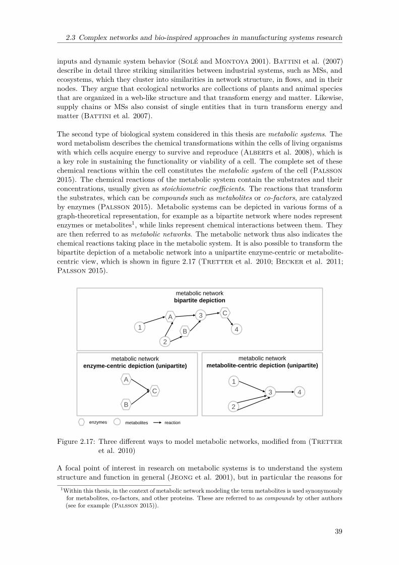
2.3 Complex networks and bio-inspired approaches in manufacturing systems research
inputs and dynamic system behavior (Solé and Montoya 2001). Battini et al. (2007)describe in detail three striking similarities between industrial systems, such as MSs, andecosystems, which they cluster into similarities in network structure, in flows, and in theirnodes. They argue that ecological networks are collections of plants and animal speciesthat are organized in a web-like structure and that transform energy and matter. Likewise,supply chains or MSs also consist of single entities that in turn transform energy andmatter (Battini et al. 2007).
The second type of biological system considered in this thesis are metabolic systems. Theword metabolism describes the chemical transformations within the cells of living organismswith which cells acquire energy to survive and reproduce (Alberts et al. 2008), which isa key role in sustaining the functionality or viability of a cell. The complete set of thesechemical reactions within the cell constitutes the metabolic system of the cell (Palsson2015). The chemical reactions of the metabolic system contain the substrates and theirconcentrations, usually given as stoichiometric coefficients. The reactions that transformthe substrates, which can be compounds such as metabolites or co-factors, are catalyzedby enzymes (Palsson 2015). Metabolic systems can be depicted in various forms of agraph-theoretical representation, for example as a bipartite network where nodes representenzymes or metabolites1, while links represent chemical interactions between them. Theyare then referred to as metabolic networks. The metabolic network thus also indicates thechemical reactions taking place in the metabolic system. It is also possible to transform thebipartite depiction of a metabolic network into a unipartite enzyme-centric or metabolite-centric view, which is shown in figure 2.17 (Tretter et al. 2010; Becker et al. 2011;Palsson 2015).
A
1
2
3
4 B
C
metabolic network
bipartite depiction
metabolic network
enzyme-centric depiction (unipartite)
metabolic network
metabolite-centric depiction (unipartite)
A
B
C
1
3 4
2
metabolites enzymes reaction
Figure 2.17: Three different ways to model metabolic networks, modified from (Tretteret al. 2010)
A focal point of interest in research on metabolic systems is to understand the systemstructure and function in general (Jeong et al. 2001), but in particular the reasons for
1Within this thesis, in the context of metabolic network modeling the term metabolites is used synonymouslyfor metabolites, co-factors, and other proteins. These are referred to as compounds by other authors(see for example (Palsson 2015)).
39

2 Related Work
the robustness of metabolic systems. An example for the outstanding robustness of cellmetabolism is its ability to carry out its normal function under mutation or deletion ofenzymes (Edwards and Palsson 2000; Stelling et al. 2002; Wilhelm et al. 2004;Smart et al. 2008) or under fluctuating metabolite concentrations (Fischer and Sauer2003).
Several authors have described striking similarities between metabolic systems and MSs.One of the first papers to suggest similarities between manufacturing units (e.g. machiningcenters) and biological cells is presented by Tharumarajah et al. (1998). They drawthe analogy that cells in biology have a chemical flow that is regulated by enzymes andhormones, which in manufacturing cells can be regarded as a material and informationflow that is regulated by coordinators and policies. Demeester et al. (2004) give adetailed description of the similarities they see in cell metabolism and MSs: both systemsoperate a production process in which inputs are transformed into outputs, exhibit complexproduction flows, and need to be fast and responsive to environmental changes. Theyfurther draw the analogies that enzymes in metabolic systems can be seen as the MSsmachines, and metabolites as material. They argue that solutions developed by metabolism,since it has been subject to evolution to its current state over a tremendous amount of time,should offer beneficial insights for MSs. Finally, they argue that MSs should be organizedas organic production systems by using the same production principles as biological cells,which they derive as customized local production, universal components, just-in-time tools,and local recycling loops (Demeester et al. 2004). Armbruster et al. (2005) also pointout similarities between biomolecular machines and industrial production, mentioning theexistence of self-organization or the stochasticity present in both systems. Within thisthesis, we consider three substantial similarities between cell metabolism and MSs, whichare summarized in figure 2.18. The system function of both systems is the transformationof either nutrients into biomass or raw materials into products. Furthermore, they bothoperate in environments that are subject to fluctuations and unforeseen events, such asdisturbances in nutrient or material supply. Lastly, both systems have to cope with internaldisturbances, such as enzyme failure or resource breakdowns.
system function system fluctuations
ce
ll
meta
bo
lism
m
an
u-
factu
rin
g
transformation of
materials into
products
transformation of
nutrients into
biomass nutrient supply
system disturbances
enzyme failure,
gene deletion
resource
breakdowns
material supply,
demand
Figure 2.18: Similarities between manufacturing and metabolic systems
In summary, both systems need to show high performance under typical environmentalconditions and, at the same time, maintain certain functions under a broad range of pertur-bations and varying conditions. Since this robustness with respect to large environmental
40

2.3 Complex networks and bio-inspired approaches in manufacturing systems research
changes is already inherent in metabolic networks, it makes them a very interesting rolemodel for MSs.
Interdisciplinary approaches between biological systems and manufacturing systemsresearch
In this section, existing research on the transfer of research on ecological and metabolicsystems to MSs is presented. The self-organization of ecological systems (Bonabeauet al. 1999), also referred to as swarm intelligence, can be defined as "any attempt todesign algorithms or distributed problem-solving devices inspired by the collective behaviorof social insect colonies and other animal societies" (Bonabeau et al. 1999). From theway how insects such as ants or bees search for food, several mathematical optimizationmodels and algorithms have been derived, for example the ant system (Dorigo et al.1996), the ant-colony optimization algorithm (Dorigo and Gambardella 1997), the beesystem (Sato and Hagiwara 1997), or the bees algorithm (Pham and Castellani 2009).These optimization models and algorithms have been applied in a manufacturing contextto traditional scheduling problems (Bonabeau et al. 1999; Chong et al. 2006; Pham et al.2007), to tackle different types of facility layout problems (Solimanpur et al. 2004; Haniet al. 2007), or to achieve autonomous control within the MS (Armbruster et al. 2006;Scholz-Reiter et al. 2008). A thorough review of further manufacturing problems solvedby approaches derived from the phenomenon of swarm intelligence is also given by Leitãoet al. (2012).
A further strand of research is analyzing the biological mechanism of evolution and clas-sification in MSs (ElMaraghy et al. 2008; Tolio et al. 2010; AlGeddawy andElMaraghy 2010). ElMaraghy et al. (2008) apply cladistics, a classification techniqueused in biological systematics, to parts of a product in MSs in order to identify new designpossibilities and alternatives for future products. It was further proposed that productsand their underlying MSs are subject to co-evolution, which is a phenomenon occurringin interdependent and symbiotic biological species (Tolio et al. 2010; AlGeddawyand ElMaraghy 2010). AlGeddawy and ElMaraghy (2010) suggest a model for theco-evolution of product design and manufacturing capabilities, which is based on thepreviously introduced cladistics. In a similar approach, Baldwin et al. (2012) applycladistics for the classification of different types of MSs, which allows them to depict theirevolutionary history.
Of equal importance for this thesis are approaches that build on the analogy betweenmetabolicsystems and MSs. In Becker et al. (2011), a unifying modeling approach to compare traf-fic, manufacturing, and metabolic systems is developed in order to show that optimizationstrategies from one domain can be successfully applied to the other domain. The networktopology, network elements, flow organization, and system dynamics of the three systemsare first compared and then analogies are drawn. All systems are finally analyzed usingthe same model, a flow control procedure derived from traffic light control (Becker et al.2011). Building up upon their analogies between cell metabolism and MSs, Becker et al.(2012) analyze several metabolic and manufacturing networks using complex networksmeasures, such as degree distribution or betweenness centrality, and compare the structuresof both networks.
41

2 Related Work
Robustness definitions and measures in biological systems
A large amount of different biological systems are generally characterized as being ro-bust (Whitacre 2012), however, as stated in section 2.3.3, the focus of this thesisconcerning biological systems is on ecological and metabolic systems. This section presentsrobustness definitions and measures from these two sub-fields of biology. As environmentalchanges or disruptions can negatively influence an ecosystem and in the worst case leadto extinction of species, a large body of research in ecology is concerned with biologicalconservation, i.e. how and when do species go extinct and what are the reasons for theinherent robustness against extinction in some ecosystems (Chapman and Reiss 1999;Levin 2009; Pocock et al. 2012). A type of ecologic system where biological conservationis extensively studied are food webs (Pimm 2002). As mentioned in section 2.3.3, theycan be depicted as a graph or network. One of the first network studies on food websby Williams et al. (2002) analyzes seven empirical networks and finds that the differentspecies are on average only two links apart, thus they characterize the networks as po-tential small world networks (despite their low clustering). These findings are coherentwith Montoya and Sol (2002), who investigate data sets of three food webs and findthe networks to exhibit high clustering and short path lengths, both characteristics ofsmall world networks. Dunne et al. (2002b) analyzed the robustness of food webs byinvestigating how the random removal of species influences the food web. They used datafrom 16 different ecosystems and measured robustness as the fraction of species that hasto be removed from the networks to result in a loss of more than 50% of the species. Theyfound that the investigated food webs exhibit a strong robustness against random removalof nodes, similar to the findings on many other real-life, scale-free networks (Albert et al.2000), and that the robustness against species removal increases with connectance (Dunneet al. 2002b). Using the same robustness measure as in their previous studies (Dunneet al. 2002b), Dunne et al. (2004) analyzed three data sets of marine food webs andfound that they display an even higher robustness to removal of species as other foodwebs. Staniczenko et al. (2010) enhance the existing approaches on food webs by notonly calculating the secondary extinctions after the removal of a species, but by rewiringnodes after the removal of a species. This procedure mimics the forming of new trophicinteractions among the remaining species after a species loss. 12 different food webs wereanalyzed by Staniczenko et al. (2010), using secondary extinction after species removalas a robustness indicator (as suggest by all previous studies). They find that certain typesof species can react as overlap species in the case of species removal, which significantlypromotes robustness of the networks. To assess the importance of a species for the overallrobustness of a food web, Jordán et al. (2007) apply 13 different centrality measures tothe trophic flows of nine different food webs. In a further study, they compare their staticcentrality measures with traditional simulations of the behavior of trophic flows in foodwebs, and find that some of the static measures show the same behavior as the traditional,dynamic measures (Jordán et al. 2008).
Another example for the interest in biological conservation and robustness in ecologicsystems are mutualistic systems, which as introduced in section 2.3.3 can also be depictedas graphs or networks. Similar to food webs, the structure of mutualistic networks hasthus been analyzed using measures from complex networks science. Jordano et al. (2003)analyzed 53 plant-pollinator and plant-seed disperser networks, which mostly showeda broad-scale degree distribution, indicating a high robustness against removal of highlyconnected nodes (targeted attacks). In their study on 37 mutualistic networks, Olesen
42

2.3 Complex networks and bio-inspired approaches in manufacturing systems research
et al. (2006) first transform the bipartite mutualistic networks into unipartite networks andthen analyze their shortest path length and clustering. They found that the characteristicsof the bipartite and unipartite networks correlate strongly and that both shortest pathlength and clustering are very low for all pollinator networks, indicating that they exhibitvery strong small-world properties (Olesen et al. 2006). A further approach by Memmottet al. (2004) analyzes the robustness of mutualistic networks to species extinction accordingto the method Dunne et al. (2002b) used for food webs. In two mutualistic networks, theyremoved pollinators at random, from most linked to least linked, and from least to mostlinked, and found that the mutualistic networks are strikingly more robust to removal ofspecies than food webs (Memmott et al. 2004). This robustness of mutualistic networksis generally attributed to the strongly nested structure of mutualistic networks (Memmottet al. 2004; Burgos et al. 2007). In contrast to measures originating from physics orcomplex networks science, such as degree distributions or node centrality, nestedness isa concept that originated from the study of island habitats (Patterson and Atmar1986; Atmar and Patterson 1993). It was originally described as the situation inwhich pollinators that interact with only a small amount of plants (specialists) are propersubsets of pollinators that interact with a large amount of plants (generalists) (Atmarand Patterson 1993). It was then shown, for example in a large-scale investigation of52 mutualistic networks by Bascompte et al. (2003), that most real world mutualisticnetworks are significantly nested.
Further biological systems where it is of interest to researchers how changes in the environ-ment or disruptions within the system affect the performance of the system are metabolicsystems. An example for changes within the environment of a metabolic system could be achange in nutrient concentration, while an example for a disruption within the metabolicsystem could be a gene mutation or a gene deletion. As explained in section 2.3.3, metabolicsystems can be modeled in a graph or network representation. The robustness of biomassproduction of metabolic systems under perturbations can be studied using flux balanceanalysis (FBA), which is a mathematical programming method that allows to analyze theflow of metabolites through a metabolic network using reconstructed in silico metabolicsystems (Orth et al. 2010). FBA was used to analyze the robustness of cellular growthin different metabolic networks under varying environmental conditions (Edwards andPalsson 2000; Segrè et al. 2002), and it was shown that the in silico predictions of themathematical models of metabolism were consistent with experimental data on the samesystems (Edwards et al. 2001; Segrè et al. 2002). Popular topological measures fromthe analysis of complex networks were also applied to analyze robustness to disruptions(e.g. lethal mutations of genes) in metabolic networks (Jeong et al. 2000). Jeong et al.(2000) study the metabolic networks of 43 organisms and observe that they are scale-freenetworks, which means they display an insensitivity to the removal of random links. Theyalso calculated the network diameter, which is the same for all 43 networks, and via asimulation study found that the diameter increases rapidly upon removal of the mostconnected nodes (Jeong et al. 2000). Barabási and Oltvai (2004) give a summary offurther complex network measures used in metabolic systems to understand the functionalorganization of the cell. A particularly interesting topological measure that has shownto be more successful in predicting the effects of gene deletions and thus the robustnessof a metabolic network compared to the measures from complex network science is thenumber of EFMs (Stelling et al. 2002; Wilhelm et al. 2004; Behre et al. 2008). EFMsare non-decomposable chemical reaction paths in the metabolic network that allow forautonomous function of the underlying organism (Schuster and Hilgetag 1994). In
43
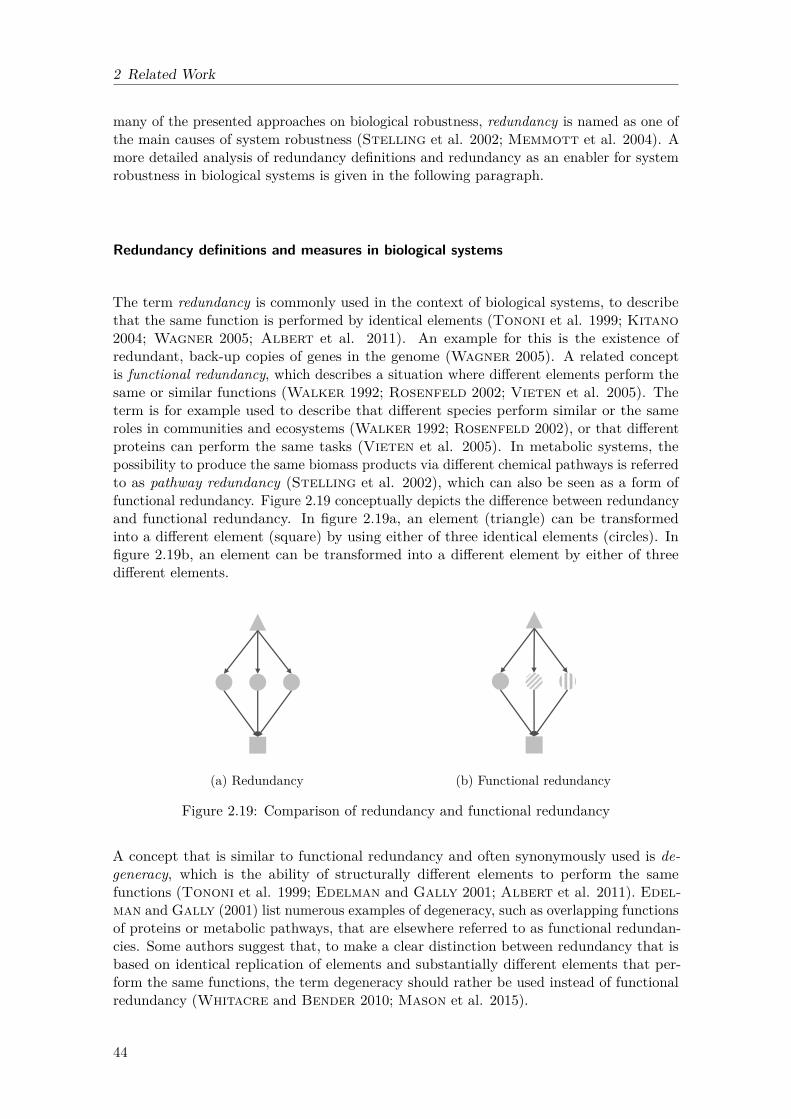
2 Related Work
many of the presented approaches on biological robustness, redundancy is named as one ofthe main causes of system robustness (Stelling et al. 2002; Memmott et al. 2004). Amore detailed analysis of redundancy definitions and redundancy as an enabler for systemrobustness in biological systems is given in the following paragraph.
Redundancy definitions and measures in biological systems
The term redundancy is commonly used in the context of biological systems, to describethat the same function is performed by identical elements (Tononi et al. 1999; Kitano2004; Wagner 2005; Albert et al. 2011). An example for this is the existence ofredundant, back-up copies of genes in the genome (Wagner 2005). A related conceptis functional redundancy, which describes a situation where different elements perform thesame or similar functions (Walker 1992; Rosenfeld 2002; Vieten et al. 2005). Theterm is for example used to describe that different species perform similar or the sameroles in communities and ecosystems (Walker 1992; Rosenfeld 2002), or that differentproteins can perform the same tasks (Vieten et al. 2005). In metabolic systems, thepossibility to produce the same biomass products via different chemical pathways is referredto as pathway redundancy (Stelling et al. 2002), which can also be seen as a form offunctional redundancy. Figure 2.19 conceptually depicts the difference between redundancyand functional redundancy. In figure 2.19a, an element (triangle) can be transformedinto a different element (square) by using either of three identical elements (circles). Infigure 2.19b, an element can be transformed into a different element by either of threedifferent elements.
(a) Redundancy (b) Functional redundancy
Figure 2.19: Comparison of redundancy and functional redundancy
A concept that is similar to functional redundancy and often synonymously used is de-generacy, which is the ability of structurally different elements to perform the samefunctions (Tononi et al. 1999; Edelman and Gally 2001; Albert et al. 2011). Edel-man and Gally (2001) list numerous examples of degeneracy, such as overlapping functionsof proteins or metabolic pathways, that are elsewhere referred to as functional redundan-cies. Some authors suggest that, to make a clear distinction between redundancy that isbased on identical replication of elements and substantially different elements that per-form the same functions, the term degeneracy should rather be used instead of functionalredundancy (Whitacre and Bender 2010; Mason et al. 2015).
44

2.4 Research Gap
Redundancy is claimed to be the cause of robustness in several biological systems. Formutualistic networks, the robustness of the systems has also been attributed to the functionalredundancy of species (Walker 1995), which also manifests itself in the nested structureof the systems (Memmott et al. 2004). Wagner (2005) name gene redundancy as oneof the main causes of robustness against mutations. It has further been argued that therobustness of metabolic systems is strongly linked to pathway redundancy (Stelling et al.2002). Chen (2008) identify redundancy, modularity, and decoupling as factors that causerobustness in metabolic systems.
2.4 Research Gap
2.4.1 Lack of robustness considerations in the design of manufacturingsystems
The existing approaches to design job shop MSs are either focused on designing a solutionthat is cost-optimal, in particular with mathematical optimization approaches to determineresource requirements (see section 2.1.3), or to create a model based on the structuraldata to analyze which MSP could potentially be reached with the design, which is doneusing queuing or simulation models (see section 2.1.3). However, streamlined, cost-optimalsystems are vulnerable to unforeseen disturbances, and MSP can easily be negativelyinfluenced. The design approaches using queuing models and simulation are used to makeassumptions about the MSP, but so far do not consider robustness of MSP when designinga MS and its resource requirements (with the exception of designing a robust product orprocess quality, see section 2.2.3).
2.4.2 Influence of redundancy on the robustness of manufacturing systemperformance
In order to design MSs so that they exhibit a robust MSP, the factors that favor or impairrobustness in MSs have to be identified. As presented in section 2.2.2, a variety of differentMSP measures are used to assess the robustness of MSs, such as flow times, WIP, ormakespan, and many models have been suggested that analyze how design, scheduling,or control can positively or negatively influence them. However, the robustness of theMSP measure lateness, which is gaining in significance in today’s customer driven markets(see section 1), has not been as intensively investigated as the robustness of other MSPmeasures yet. Especially factors that favor or impair the robustness of lateness have notbeen subject of interest in the manufacturing context so far.
Judging from the presented approaches from complex network science and biology, redun-dancy is seen as a key enabler of system robustness in these domains (see section 2.3.3).What is regarded as a redundancy in a manufacturing context has not been clearly definedyet (see section 2.2.7), least has the influence of redundancy on robust MSP with regard tolateness been analyzed. In order to subsequently analyze the relationship between redun-dancy and robustness in MSs, a definition of redundancies in MSs needs to be establishedand a measure found to analyze the potential influence of redundancy on robust MSP.
45

2 Related Work
2.4.3 Motivation for using interdisciplinary methods for robust manufacturingsystems design
The information that is available at the design stage of job shop MSs is limited to informationregarding the system structure, such as products, their characteristics, the subsequentlynecessary manufacturing processes and machines, and the potential material flows (seesection 2.1.3). The models created for MSD are a means to predict the potential systembehavior. However, the queuing and mathematical optimization approaches used todetermine resource requirements in job shop MSs lack applicability to more realistic,large-scale and complex MSs, as they are limited to relatively small sizes of MSs (seesection 2.1.3). Likewise, forming a simulation model that adequately depicts a a large-scale, complex MS is a time and resource consuming task, and the simulation modelmight not adequately depict the system. As demonstrated in section 2.3.1, both complexand biological systems share striking similarities with MSs. As metabolic and ecologicalsystems, MSs face fluctuating environmental influences and internal disruptions and thusshare the common challenge to maintain a high level of efficiency for a variety of differentconditions (see section 2.3.3). Similarly, MSs exhibit the typical properties of complexnetworks (see section 2.3.2). The methods developed in both domains seem to be able totackle the previously identified shortcoming of methods traditionally used in manufacturingresearch for MSD (i.e. queuing and mathematical optimization), as they are made forlarge-scale, complex systems. Different analogies between ecological, metabolic and MSshave already been described in the past (see section 2.3.3), yet only in few works did theseanalogies ever evolve past a conceptual state. However, transferring methods used foranalyzing ecological or metabolic systems can result in gaining new insights, as was shownfor example by Becker et al. (2011). Especially nestedness and EFM analysis presentedin section 2.3.3 have been outstandingly successful in their respective disciplines. Both arecalculated solely based on topological information about the respective systems, but stillshow a striking relation to system robustness. They are able to predict the dynamic systembehavior based on the structural characteristics of the respective system. Moreover, theyimplicitly consider different forms of redundancies (functional and pathway redundancy)and thus, due to the assumed positive influence of redundancy on robustness, seem suitableto measure and analyze system robustness based on the structural data in MSs.
46

3 Analyzing the relationship betweenrobustness and redundancy inmanufacturing systems
In the third chapter, the relationship between robustness and redundancy in MSs is analyzed.Therefore, the underlying measures for robustness and redundancy used within this thesis aregiven in section 3.1 and section 3.2, based on measures that were introduced in section 2.2.1and section 2.3.3. Robustness is measured as the change of a MSP measure in perturbedand unperturbed situations as suggested by Alderson and Doyle (2010). Redundancyis measured as two different types of machine redundancy, based on the differentiationbetween duplicate redundancy and functional redundancy in biological systems (Kitano2004; Walker 1992), which was introduced in section 2.3.3. Subsequently, the potentialrelationship between robustness and redundancy is described in section 3.3. Consideringfindings from other real world systems like biological systems where redundancy is supposedto have a positive effect on system robustness (Stelling et al. 2002), it is assumed that therelation between the two concepts is also positive in MSs. Furthermore, it is investigatedwhether two measures from complex network science - node degree and betweenness centrality- which show a significant relation to robustness in other real world networks (Albertet al. 2000) as described in section 2.3.2, are also related to robustness in MSs. To analyzethe relation of robustness with redundancy and complex network measures, simulationmodeling is chosen as a research method, as it seems to be the only method fit to copewith the complexity of job shop MSs and the dynamic system behavior necessary tostudy robustness, which necessitates an analysis of MSs in perturbed and unperturbedconditions. Thus a simulation study is conducted in section 3.4. The section first gives ashort introduction to the general procedure of simulation modeling and criteria for valid andrealistic simulation models in MSs ( 3.4.1). To build the simulation model as realisticallyas possible, a large range of different MS configurations are created with a mathematicaloptimization approach for cost-optimal resource requirements design in MSs by Bardand Feo (1991) ( 3.4.2). The created MS configurations display different amounts ofmachines, redundancy, and network characteristics. Subsequently, the simulation modeland the experiments conducted with it are described in detail and robustness (defined asthe behavior of the MSP lateness in perturbed and unperturbed scenarios) of each MSconfiguration is measured ( 3.4.3). Robustness of each MS configuration is then correlatedto the redundancy and complex network characteristics of the respective MS configurations( 3.4.4). A significant positive linear and rank correlation between robustness and one ofthe machine redundancy measures is observed, while no significant linear correlation isfound between node-degree or betweeness centrality and robustness in MSs. As a last stepof this chapter, the intermediary results are summarized and discussed in section 3.5.
47

3 Analyzing the relationship between robustness and redundancy in MSs
3.1 Defining and measuring robustness in job shopmanufacturing systems2
As stated in many of the works cited in section 2.2, robustness is a concept or an abstractthat cannot be observed or measured directly (Félix and Wagner 2008; Alderson andDoyle 2010; Mondal et al. 2014). It is rather a characteristic of an object or systemand thus is measured indirectly from the performance of the object or system under study.The measure for robustness within this thesis is based on the definition of a robustnessmeasure given by Alderson and Doyle (2010) (see section 2.2.1), who state that tomeasure robustness, the system under study, the property that should be robust, the set ofperturbations against which the system should be robust and an invariance measure needto be defined. Many of the presented measures for robustness in a manufacturing context(section 2.2.2) incorporate the four aspects of a robustness measure set up by Aldersonand Doyle (2010), without explicitly referring to them. As an example, in their approachfor robust scheduling, Goren and Sabuncuoglu (2008) define the system under study(production schedule), the properties that should be robust (makespan, total flow time,total tardiness of jobs), the invariance measures (expected sum of absolute deviationsin job completion times), and the perturbations (random machine breakdowns) againstwhich the property should be robust. Yet none of the approaches that give a thoroughdefinition of robustness in the manufacturing context are concerned with overall MSP as theproperty under study. On the other hand, some of the existing definitions for robustness ina manufacturing context only measure static network values (e.g., shortest path length (Liuet al. 2011)), which is a shortcoming as networks in a manufacturing context are not staticbut change over time. When MSs are represented as machine-material flow networks, thelinks (material flows) between the nodes (machines) can vary drastically depending on theproducts ordered in the analyzed time-span, as different machines and material flows areactive. This has also been shown for example in social communication networks, where theroles of the different nodes in the network change over time (Braha and Bar-Yam 2006).Thus definitions for robustness in a manufacturing context that are only based on averagenetwork values from a graph theoretical depiction of the MS do not seem to be sufficientmeasures. As the significance of certain nodes for the robustness changes dynamically,integrating a time-component into the robustness definition is crucial.
In the following section, the system, performance, perturbations, and invariance measuresof the robustness measure suggested within this thesis are explained. The system understudy is the MS of a manufacturing organization. The property or function that shouldbe robust in the face of perturbations usually is declared to be a specific manufacturingperformance indicator, for which the abbreviation MSP was introduced earlier. The MSPof a MS does usually not stay on an exact same level, but varies over time (t), evenif no unplanned perturbations (p) occur, which is conceptually depicted in figure 3.1a).In a realistic manufacturing environment however, unplanned perturbations occur andnegatively influence the MSP (MSP ′), as shown in figure 3.1b.
As reviewed in section 2.1.2, different performance measures exist to assess MSP (Bititci1995; Ghalayini et al. 1997; Gomes et al. 2004; Hon 2005; Chen and Huang 2006;Gomes et al. 2006), with different categorizations such as cost, quality, or time performancemeasures (Hon 2005; Chryssolouris 2006). As stated in the introduction and scope of
2Parts of this section have been published in similar form in (Meyer et al. 2013).
48

3.1 Defining and measuring robustness in manufacturing systems
MSP
t
(a) MSP in unpterturbed situation
MSP´
t
p2 p1 p3
(b) MSP under unplanned perturbations
Figure 3.1: Conceptual depiction of MSP in a MS
this thesis (see section 1), the developed models and analysis focus on time performancemeasures, as these are considered most crucial for customer satisfaction in today’s buyermarkets. In particular, the focus will be on lateness, as introduced in section 2.1.2.Lateness (l) can be evaluated for every single job, and for every single order. In general, itis measured as the difference between actual end time (ea) and planned end time (ep) ofjobs or orders (Nyhuis and Wiendahl 2009; Pinedo 2012; Framinan et al. 2014).
l = ep − ea (3.1)
In case a job or order is late, the difference is a positive value, in case a job or order isearly, the difference is a negative value. Both positive and negative lateness values areregarded as negative for the MS as both can incur additional costs: early jobs or orderscause higher inventory costs as there is more inventory than necessary and late jobs ororders cause a decrease in MSP towards the customer as due dates are missed. In additionto this general definition, several more detailed lateness specifications are depicted infigure 3.2. Input lateness (lin) is the deviation of the actual start date of a job or order(sactual) from the planned start date of the job or order (splanned). Similarly, the outputlateness (lout) is the deviation of the actual end date of a job or order (eactual) from theplanned end date of the job or order (eplanned). Relative lateness (lrel) of a job or order iscalculated as the difference between the actual start date and the planned end date. In
time
planned throughput
job 1 actual throughput
job 1
sjplannned ejplanned sjactual ejactual
lout lrel lin
Figure 3.2: Different types of lateness, modified from (Nyhuis and Wiendahl 2009)
addition to job or order lateness, a depiction of lateness is also possible on a workstationor MS level. Workstation lateness can be calculated as the average lateness of all jobs
49

3 Analyzing the relationship between robustness and redundancy in MSs
or orders that are treated on a workstation, while MS lateness can be calculated as theaverage lateness of all jobs or orders within the MS. When an average of the job, order,workstation, or MS lateness is calculated (either on the workstation or MS level), theabsolute values can be used to prevent negative and positive lateness values from averagingout, which is called the average absolute lateness.
As also depicted in figure 3.1b, different perturbations can have a different impact on MSP.This impact depends on the type or duration of the perturbation, a machine breakdowncould for example lead to a higher and longer decrease of MSP than a shortage of a certainmaterial. As reviewed in section 2.1.4, a multitude of different perturbations exist in amanufacturing context. In this work, the perturbation against which the performancemeasure should be robust is a machine breakdown.
The invariance measure for robustness in this thesis is the ratio that results from thecomparison of the MSP in a scenario without perturbations to the MSP in a scenario withperturbations, where perturbations are machine breakdowns. As the focus of this thesis ison the MSP lateness, robustness will be calculated as the ratio of lateness in an unperturbed(l) and a perturbed (l ′) scenario, where perturbations are machine breakdowns.
r =ll ′
(3.2)
A similar invariance measure has previously been suggested in a manufacturing context forexample by Meyer et al. (2013), who measure robustness as the ratio of four differentMSP measures (utilization, due date reliability, throughput-time, lateness) in scenarioswith and without capacity fluctuations. Similarly, Putnik et al. (2015) measure robustnessin a MS as the ratio between the drop in production rate of the MS under perturbationand the production rate in a stationary state. Another possible invariance measures forrobustness in a MS context is to take the standard deviation of a MSP measure, whichwas proposed for example by Leon et al. (1994) in their collection of robustness measuresfor robust scheduling. In contrast to invariance measures such as the standard deviation,the ratio-based measure chosen in this thesis makes it possible to compare the robustnessvalues of different MSs, as it is a normalized measure. Although the chosen measure canserve to compare different MS, its shortcomings are that it is only applicable if a modelof the MS under study exists, as it is not feasible to declare and observe perturbed andunperturbed scenarios in real MSs or when recorded feedback data is analyzed.
3.2 Defining and measuring redundancy in job shopmanufacturing systems
This section gives a definition of what is considered to be a redundancy in the contextof job shop MSs. Similar to the definitions from biological contexts, redundancy in MSsis the existence of exact identical copies of an element that fulfill the same function,while functional redundancy in MSs is considered to be the existence of non-identicalelements that are able perform the same functions. Elements in this context refer toelements in the MS, for example resources such as machines, equipment, or workforce,which were already introduced in section 2.1.1. The existence of several machines of thesame type is very common in job shop MSs, for example when more capacity than one
50

3.2 Defining and measuring redundancy in job shop manufacturing systems
machine can offer is needed. Likewise, machines can also fulfill what is seen as a functionalredundancy in biology: flexible machining centers in FMS can for example sometimesperform the same processing steps (e.g., milling, drilling), although they are not exactduplicates of each other, and can thus be regarded as a functional redundancy. Furtherphysical elements that can be regarded as redundant elements are the different types ofmaterial in MSs. It is common for raw-materials that identical copies are kept in storage,for example a company that uses steel profiles as raw materials will usually have more thanone of each type on stock, which can be seen as a redundancy. However, a raw materialcould also be seen as functionally redundant, if it can be used instead of another type of rawmaterial. In reality, only few examples can be found where this is actually the case. Thesame holds true for sub-assemblies or semi-finished parts: they can be redundant, if severalidentical copies of them are kept in stock, or they can be regarded as functionally redundantif they can replace structurally different sub-assemblies or semi-finished parts in a product.Finished products can be seen as redundant as well, if in case of a make-to-stock strategy acompany keeps an inventory of finished goods. Transport and handling equipment can alsoexist as duplicates, or they can be used to process different materials or parts and thuscan be seen as functionally redundant. Keeping duplicate raw-materials, sub-assemblies,or products is conceptually similar to safety-stock, which was introduced as a means tocounteract the negative impact of disturbances on MSP in MSs in section 2.1.4. Theredundancy categorization is summarized in table 3.1.
resource redundancy functional redundancymachine duplicate machines different machines can fulfill
same functiontransport & handling equipment duplicate transport & handling
equipmentdifferent transport & handlingequipment can fulfill same func-tion
workforce duplicate workers on the sameskill level
differently skilled workers canfulfill same function
raw-materials duplicate raw materials different raw materials can fulfillsame function
sub-assemblies duplicate sub-assemblies different sub-assemblies can ful-fill same function
final products duplicate final products -
Table 3.1: Redundancy and functional redundancy in manufacturing systems
Within this thesis and the following analysis, the focus will be on machine redundancyand machine functional redundancy. Therefore the differences and similarities betweenthese identified redundancy types and related other terms in MSs research are discussedin detail in the following, and a measure for each of the concepts is given. Both machineredundancy or machine functional redundancy allow for the existence of alternative routesfor a product: if several duplicate machines of one type exist, products can be treatedon either of them, and each choice would represent a separate path. Likewise, if twomachines are not identical but can perform the same manufacturing process, the productcould be treated on either of them and each choice again would represent a unique path.Alternative product routes are conceptually the same as pathway redundancy found inmetabolic networks. They are a very distinct characteristic of job shop MSs or FMS, andare not present for example in cellular manufacturing systems, where a set of productfamilies is assigned to a specific cell with a dedicated routing.
51

3 Analyzing the relationship between robustness and redundancy in MSs
The definition of machine redundancy as duplicate machines needs to be related to theaspect of machine capacity (for a definition see section 2.1.1). A machine usually has adefined capacity, measured in shifts, hours, work content etc., and the number of machines(and thus its capacity) in a job shop MS is usually carefully determined according to thecapacities needed (see section 2.1.3). In case the demand for products and their relatedmanufacturing processes exceeds the capacity of a machine, another one or several ones ofthe same type need to be installed. So having several redundant machines in the MS doesnot necessarily mean that excess capacity is held. We measure machine redundancy (mr)in a MS as the average amount of machines m of type i.
mr =1n
n∑i=1
mi (3.3)
The prerequisite for machine functional redundancy is that machines are able to processseveral different manufacturing processes. This ability of a machine "to perform morethan one type of processing operation efficiently" (Das and Nagendra 1993) is alsoreferred to as machine flexibility. In the context of research on flexibility in MSs, machineflexibility is seen as an enabler for routing flexibility, which is the "ability of the system tomanufacture products via a variety of different routes" (Das and Nagendra 1993). Thisis coherent with the previously given definition that machine functional redundancy actsas an enabler of alternate production routes. A vast amount of different measures havebeen suggested for machine flexibility and routing flexibility in the past. The number ofdifferent manufacturing operations a machine can perform is among the simplest definitionsto measure machine flexibility (Sethi and Sethi 1990), and it will be used within thisthesis to measure machine functional redundancy (mf r). It is measured as the averageamount of manufacturing processes p a machine m can fulfill (mp).
mf r =1n
n∑p=1
mp (3.4)
For routing flexibility, the most important definitions include the number of routes perproduct or average number of available routes for each part type, which are presentedtogether with other measures in an extensive review by Yu and Greene (2009). Inaddition to the many existing definitions for machine and routing flexibility, the effect ofboth on different MSP measures has also been extensively studied (Das and Nagendra1993; Caprihan and Wadhwa 1997; Chan 2001; Ali and Wadhwa 2010). In Das andNagendra (1993), the influence of routing flexibility on flow time and WIP inventory inFMSs is studied using a simulation model. The authors find that increased routing flexibilityleads to shorter lead times and decreased WIP inventory. Caprihan and Wadhwa (1997)analyze the influence of routing flexibility in FMSs on the MSP measure makespan, using alsoa simulation study. Their results indicate that routing flexibility is not always beneficial, asthey identify an optimal flexibility level above which system performance deteriorates. Chan(2001) also analyze the effect of routing flexibility on makespan in FMSs using a simulationstudy, but also incorporate an analysis of robustness against machine failure, using Taguichimethods. They conclude that routing flexibility is especially important for MSs in whichmany disruptions occur. In Ali and Wadhwa (2010) the influence of routing flexibilityand other parameters on the performance measure makespan is analyzed in a FMS using asimulation study combined with Taguichi methods. Similarly to Caprihan and Wadhwa(1997), the authors find that routing flexibility does not significantly increase performance,and that large flexibility levels even worsen performance.
52

3.3 Potential relationship between robustness and redundancy
Many of the presented approaches show that routing flexibility, which is only enabled bymachine flexibility, increases MSP (Das and Nagendra 1993; Caprihan and Wadhwa1997; Chan 2001). Yet none of the approaches so far studied the influence of routingflexibility on the robustness of MSP, although many works concerned with flexibility inmanufacturing claim that flexibility - and in particular routing flexibility - acts as anenabler of robustness (Swamidass and Newell 1987).
3.3 Potential relationship between robustness and redundancy
In many real world systems, for example in metabolic or ecological systems, redundancy inpathways (Stelling et al. 2002) or species (Memmott et al. 2004; Burgos et al. 2007)was found to have a positive influence on robustness. In a manufacturing context, theinfluence of redundancy on robustness in MSs (as defined in section 3.1) can also be assumedto be positive, which can be illustrated with the following example: when a production orderis released to the shop floor and the raw material needed for production is not present dueto a delivery delay from the supplier, the planned due dates for the production order usuallycannot be met, which results in an increased lateness. In case redundant raw materials hadexisted, the delays could be shortened or prevented completely. Similarly, if unforeseenmachine breakdowns occur and no alternative routes exist, production orders will not beable to meet their originally planned due dates as they pile up in front of the machine underbreakdown. If machine or machine functional redundancy had existed, the productionorder could have used an alternative routing and could have been treated on a differentmachine. Thus lateness would not be negatively influenced, which can be seen as a highrobustness of lateness against machine breakdowns. From a holistic point of view, it is notknown how successful redundancy in MSs can buffer against or reduce the negative effectson MSP incurred by disturbances: a disturbance can often affect subsequent activities, i.e.it propagates through the system. In case of a machine breakdown, this means for examplethat the production order is delayed at a certain machine under breakdown, but carriesthis delay through the entire MS, as it will also not meet the initially planned due dateson subsequent machines. It is a core assumption of this thesis that redundancy (machineredundancy and machine functional redundancy, as defined in section 3.2) has a positiveeffect on robustness (robustness of the MSP measure lateness against machine breakdowns,as defined in section 3.1). This relationship is conceptually depicted in figure 3.3, whereincreased redundancy in a MS results in increased robustness. However, it is not knownhow exactly the relationship between the two variables behaves, which is why two differentpotential relationships are shown as examples in the figure. The relationship could forexample be depicted by a linear function, where both values increase proportionally, orby an exponential function, where one value increases by a constant factor with each stepof the other value. One of the aims of this thesis is to investigate the above describedrelationship between robustness and redundancy in MSs.
In general, the ways to exploratively analyze a system or its behavior are experimentswith the actual system or experiments with a model of the system (Law 2014). In thescientific fields where similar relations are of interest (e.g. metabolic or ecologic networks)such relationships are usually investigated by analyzing a variety of different real worldsystems. This is possible as in these domains, large, publicly available databases containingdata sets of real world systems exist, for example the KEGG database (Kanehisa and
53

3 Analyzing the relationship between robustness and redundancy in MSs
Goto 2000). Original data sets are also often published completely, as for example usedin Bascompte et al. (2003). Similar to approaches in other real world systems, therelationship between robustness and redundancy should not only be analyzed in one singleMS, but in several MSs with different characteristics, to be able to draw generalizableconclusions. However, conducting experiments with real MSs is an unfeasible option, as itwould be too time consuming to gather data for a statistically significant amount of realworld MSs. Moreover, manufacturing organizations are usually reluctant in providing dataconcerning their MSs, as they see it as a core competency of their business. Thus it waschosen to use a model of MSs to analyze the relation between robustness and redundancywithin this thesis. Different types of models exist to analyze MSs, for example processor mathematical models, of which the latter can be further distinguished into analytical orsimulation models (Brandimarte and Villa 1995; Altiok and Melamed 2010; Law2014). Analytical models, such as queuing models (Buzacott and Shanthikumar 1992;Papadopoulos et al. 1993; Gershwin 1994) or mathematical optimization models (alsoreferred to as operations research) (Brandimarte and Villa 1995; Rao et al. 2010),result in exact answers. However, they are usually restricted to small sizes of MSs andnot applicable to more complex systems, in which it is "impossible to find an analyticalrelationship between decision variables and performance measures" (Brandimarte andVilla 1995). So if the MSs to be analyzed are complex, an analytical solution can beunfeasible or result in unreasonably high modeling efforts (Law and McComas 1987;Brandimarte and Villa 1995; Law 2014). As job shop MSs are seen as complexsystems with a multitude of different resources and connections between the resourceswithin this thesis (see sections 2.1.1 and 2.1.4), an analytical model seems unfeasible forthe modeling task. Therefore a simulation model was chosen to analyze the relationshipbetween robustness and redundancy in MSs. In the following section, the specific simulationmethod employed and its applicability in a manufacturing context are presented in moredetail.
redundancy
robu
stn
ess
Figure 3.3: Conceptual depiction of the potential relationship between robustness andredundancy in MSs
54

3.4 Simulation analysis of the relation between redundancy and robustness in MSs
3.4 Simulation analysis of the relation between redundancy androbustness in manufacturing systems
3.4.1 Simulation as a research methodology in manufacturing systemsresearch
As mentioned in the previous section, a simulation model of a MSs serves as a surrogate forconducting actual experiments or analysis in a real MS, as these are often infeasible or notcost-effective (Law andMcComas 1987; Law andMcComas 1998; Law 2014). Simulationin general is a well-established research method within the domain of MS research, and isused for design and operation of MSs (Iwata and Oba 1984; Law and McComas 1987;Alting et al. 1988; Law and McComas 1998; Miller and Pegden 2000; Smith 2003;Jahangirian et al. 2010; Silva et al. 2014; Negahban and Smith 2014). For the generalprocedure of conducting a simulation study in a manufacturing context, various approacheshave been suggested in literature. Several authors split the general simulation procedureinto three steps: a conceptional or design phase, a development or implementation phase,and a deployment or analysis phase (Chance et al. 1996; Fowler 2004; Montevechi etal. 2007). In the design or conceptional phase, the goals of the modeling process, the systemunder study, as well as the participants involved in the model design are determined. It alsoincludes the construction and validation of a first conceptual model. This is followed by thedevelopment or implementation phase, in which based on the conceptual model, a modelingapproach is chosen. A computer model is then built, and verified and validated. In the lastphase, the deployment or analysis phase, experiments to be executed with the model aredesigned, the simulation model is executed, and the results are analyzed (Chance et al.1996; Fowler 2004; Montevechi et al. 2007).
The specific simulation method chosen within this thesis is a discrete-event simulation(DES) model. DES is a simulation method used to model the behavior of a system asa discrete sequence of events, which mark a change of state in the system (Altiok andMelamed 2010; Law 2014). In a manufacturing context, an event could be the arrival ofa new job at a machine or the end of processing of a job on a machine. An experimentdescribes the configuration of the MS or the scenario which is analyzed with the simulationmodel (Altiok and Melamed 2010). Miller and Pegden (2000) give a summary of thefeatures a DES model of a MS can comprise, which are for example resources, materialhandling devices, control logic, workstation logic, buffers, as well as order or process plans.Variables or parameters like these can be changed along the different experiments conductedwith the simulation model. The simulation clock is a variable which gives the currentvalue of simulated time (Law and McComas 1987; Law 2014). The run time is the totalnumber of time units for which the simulation model is run. If the time units are forexample measured in days, the total run time of the model is a specific number of days.The first values of simulated time in a simulation run are often described as the warm-upperiod of the simulation model (Law and McComas 1987; Chance et al. 1996; Altiokand Melamed 2010; Law 2014). Several authors argue that performance values measuredduring the warm-up period should be disregarded, as the simulation model needs a certainramp-up time to get into a state of steady functioning (Law 2014).
DES has been used in a manufacturing context for analyzing the impact of different factors,for example scheduling or dispatching rules, inventory policies, or characteristics such as
55

3 Analyzing the relationship between robustness and redundancy in MSs
flexibility and self-organization, on MSP (Schroer and Tseng 1988; Das and Nagendra1993; Nagarur and Azeem 1999; Holst 2001; Usher 2003; Koh and Saad 2003; Longoet al. 2012; Sharma and Garg 2012). Das and Nagendra (1993) used a simulationstudy to analyze the influence of routing, machine, and product-mix flexibility on theMSP measures average flow time and WIP inventory. Similarly, Nagarur and Azeem(1999) analyze the influence of machine flexibility and part standardization on the MSPmeasures makespan, average machine utilization, and factor productivity using a DES. Afurther study analyzes the impact of alternative plans and thus alternative routes on theMSP measures tardiness, also employing DES as an analysis method (Usher 2003). Theexisting simulation studies on flexibility however do not focus on analyzing the MSP inunperturbed and perturbed situations (for example under machine breakdowns). Theymerely depict the behavior of MSs under normal operating conditions, and no conclusionsregarding robustness of MSP can be drawn from them. However, DES can easily be usedto also analyze the impact of disruptions on the MSP performance. This was for examplesuggested by Koh and Saad (2003), who analyze the influence of machine breakdownson late deliveries using DES, or by Padhi et al. (2013), who analyze the impact of productionline disturbances on production efficiency under different levels of cycle time, operatorefficiency, and automation using a DES model. A recent study by Putnik et al. (2015)uses a DES to analyze the robustness of the production rate with regard to perturbations incustomer demand. As the analysis of the relationship between robustness and redundancyis conceptually similar to the previously presented applications of DES for analyzing theinfluence of different factors on MSP measures, it is seen as a suitable research method forthis thesis.
Most simulation approaches in MSs especially stress the importance of model verificationand validation. In general, simulation model verification means ensuring that the simu-lation model produces a correct output given a specific input (Kleijnen 1995; Carson2002; Sargent 2005; Rabe et al. 2008; Law 2014), which can also be expressed as"ensuring that the computer program of the computerized model and its implementationare correct" (Sargent 2005). Model validation on the other hand serves to determinewhether the simulation model is an accurate and realistic representation of system that isbeing studied (Kleijnen 1995; Carson 2002; Rabe et al. 2008; Sargent 2005; Law2014). In addition to being verified and valid, a simulation model also needs to be credible,which means that decision makers and experts involved in the design and use of the modelaccept it as correct (Balci 1989; Law 2009). An overview of validation techniques andcredibility criteria for simulation models, for example comparisons to other models thathave been validated or expert opinion validation, is given by Balci (1990) or Sargent(2005). In Carson (2002), a review of different modeling errors, for example data orlogic modeling errors, that should be avoided in order for simulation models to be valid,are summarized. However, it also has to be stressed that a complete validation of anysimulation is never possible (Law 2014).
Several authors summarize criteria for the validity, credibility, and quality of DES modelsspecifically tailored for a manufacturing context (Law and McComas 1987; Chanceet al. 1996; Law and McComas 1998; Fowler 2004; Wenzel et al. 2007; Rabe et al.2008). The importance of considering a warm-up period in MS simulations is stressed andsuggestions for the length of warm-up periods (around 10-15% of total run time) are givenby several authors (Law andMcComas 1987; Chance et al. 1996). It is further stressed inliterature that the length of each simulation run and the number of independent simulation
56
3.4 Simulation analysis of the relation between redundancy and robustness in MSs
runs should be chosen appropriately, with the number of simulation runs ranging between3 to 10 runs in many approaches in MSs research (Law and McComas 1987; Law andMcComas 1998; Chryssolouris et al. 2013). Fowler (2004) state that incorporationof detail on the MS may increase the credibility of a simulation model, however an excessivelevel of detail can render a model hard to build, debug, understand, deploy, and maintain.In the following, a DES model is set up to analyze the potential relationship betweenrobustness and redundancy in MSs.
3.4.2 Configuration of realistic exemplary manufacturing systems
The goals for the use of simulation within this thesis have been described in section 3.3.Following the procedure for building simulation models introduced in the previous section,this section starts with the presentation of the MSs to be analyzed. Many approaches in MSsresearch that investigate general properties of MSs with a simulation model use minimalexamples or minimal models of MSs in their analysis (for example Koren et al. (1998),Scholz-Reiter et al. (2005), Chryssolouris et al. (2013), and Blunck et al. (2014)).In these papers, a minimal model in a MS context means that the studied MSs consist ofonly a small amount of resources, e.g. three to ten resources. In Koren et al. (1998), theinfluence of the configuration of a MS (serial line or multiple parallel lines) on differentMSP measures is analyzed using a Monte Carlo simulation on six minimal models of MSconfigurations, each consisting of six machines. Similarly, Scholz-Reiter et al. (2005)study the effects of autonomous control on different MSP measures, using a simulationmodel of a MS that contains nine machines and three different product types. Anotherexample of the use of a minimal model to analyze the effects on MSP is an approachby Chryssolouris et al. (2013), in which the trade-off between flexibility and complexityin MSs is analyzed in a MS that consists of ten products and ten resources. Blunck et al.(2014) use minimal models of flow shops consisting of five work stations per operatingstep, of which there are also five, to test improvement heuristics for manufacturing systemsdesign. Minimal models are for example commonly used in the study of metabolic systems,where minimal metabolic network models are used for computationally simulating andpredicting the behavior of the real world metabolic systems (Palsson 2015). Minimalmodels can be beneficial as they reduce complexity and can thus lead to gaining universalunderstandings and insights of the functioning of various complex systems (Battermanand Rice 2014). However, as a large amount of published case study data indicates, job orflow shop MSs can easily consist of between 20 to 200 resources and manufacture between20 to more than 1000 different products (Rovithakis et al. 2001; Molleman et al.2002; Yang et al. 2004; Meyer et al. 2013; Becker and Meyer 2014). Furthermore, adescription of how the capacity or layout of the networks were decided upon is lacking inmost minimal model approaches in MS research. In Blunck et al. (2014) for example,capacities of all resources are set to a value of 1 for each resource in general. This was alsoobserved by Alhourani (2016) who criticize minimal models in the MS context for oftenusing unrealistic infinite capacities. Thus it is doubtful whether the results of simulationstudies based on minimal models of MSs are valid and credible (as defined in the previoussection 3.4.1), as it can be argued that they do not represent realistic MSs.
Within this thesis, the MSs in the simulation study should be representative for a broadrange of different job shop MSs and be as realistic as possible, to ensure credibility of themodel. Instead of focusing on one specific MS or on MSs with only a small amount of
57

3 Analyzing the relationship between robustness and redundancy in MSs
resources, the results should be valid for job shop MSs with different amount of resources,different amount of products to be manufactured, and different amounts of redundancy.To create such a broad range of MSs artificially but yet realistically, a MSD approach forjob shop MSs from manufacturing research literature is chosen. The amounts and types ofresources that are adequate for a certain product demand and available types of resourcesare determined by a mathematical optimization approach suggested by Bard and Feo(1991) (see also section 2.1.3). Their optimization model was initially suggested to determinethe investment cost-optimal machine requirements for job shop MSs in the design phase,when only information about the products and their required manufacturing processesis available. According to the model by Bard and Feo (1991), a MSs configurationis determined based on six input variables, which are the different product types to beproduced (k), the demands for the product types (dk ), the amounts of each manufacturingprocess i needed to manufacture each product type k (bik ), the efficiencies with which eachmachine type j can perform a manufacturing process i (ai j), and the discounted costs ofeach machine type j (cj). Table 3.2 summarizes the variables. An exemplary depiction ofvalues for these input variables was already given in section 2.1.3, table 2.2.
ki 1 2 . . . m1 b11 b12 . . . b1m
2 b21 b22 . . . b2m...
......
. . ....
n bn1 bn2 . . . bnm
dk d1 d2 . . . dm
(a) Process-Product Data
ji 1 2 . . . o1 a11 a12 . . . a1o
2 a21 a22 . . . a2o...
......
. . ....
n an1 an2 . . . ano
cj c1 c2 . . . co
(b) Process-Machine Data
Table 3.2: Input data to determine the machine requirements according to Bard and Feo(1991)
In order to create a broad range of different MS configurations with varying characteristics,three of the six input variables, namely the number of manufacturing processes in theMS (i), the number of different products to be manufactured (k), and the number ofmachine types (j) are varied. In addition to that, another variable that is not explicitlymentioned in the model by Bard and Feo (1991) is introduced, the process flexibility of amachine (f ). It is defined as the amount of different processes a machine of type j can fulfilland is introduced in order to create configurations where machine functional redundancywill exhibit different values. Process flexibility f is measured by the percentage of overallexisting processes a machine can fulfill: if 20 different manufacturing processes exist and amachine can fulfill 10 of these processes, its process flexibility is 0.5. The variables and thevalues they can take are summarized in table 3.3. The values have been chosen to representMSs with low, medium, and high amount of the different variables, and are coherent withdata of real MSs found in case studies on number of processes, products, and machinetypes per MS (see for example Rovithakis et al. (2001), Molleman et al. (2002), Yanget al. (2004), Meyer et al. (2013), and Becker and Meyer (2014)). Since the resourcerequirements are dimensioned with a mathematical optimization model, too large valuesfor the variables are likely to result in a long run-time of the model, which is why MSswith an extreme product variance (larger than 50) and an extremely diverse amount ofdifferent manufacturing processes (larger than 20) have been excluded from the analysis.
58
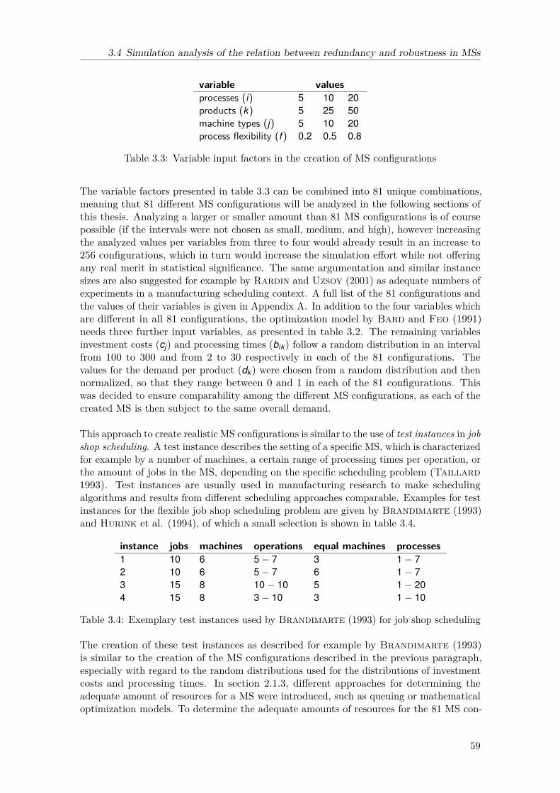
3.4 Simulation analysis of the relation between redundancy and robustness in MSs
variable valuesprocesses (i) 5 10 20products (k) 5 25 50machine types (j) 5 10 20process flexibility (f ) 0.2 0.5 0.8
Table 3.3: Variable input factors in the creation of MS configurations
The variable factors presented in table 3.3 can be combined into 81 unique combinations,meaning that 81 different MS configurations will be analyzed in the following sections ofthis thesis. Analyzing a larger or smaller amount than 81 MS configurations is of coursepossible (if the intervals were not chosen as small, medium, and high), however increasingthe analyzed values per variables from three to four would already result in an increase to256 configurations, which in turn would increase the simulation effort while not offeringany real merit in statistical significance. The same argumentation and similar instancesizes are also suggested for example by Rardin and Uzsoy (2001) as adequate numbers ofexperiments in a manufacturing scheduling context. A full list of the 81 configurations andthe values of their variables is given in Appendix A. In addition to the four variables whichare different in all 81 configurations, the optimization model by Bard and Feo (1991)needs three further input variables, as presented in table 3.2. The remaining variablesinvestment costs (cj) and processing times (bik ) follow a random distribution in an intervalfrom 100 to 300 and from 2 to 30 respectively in each of the 81 configurations. Thevalues for the demand per product (dk) were chosen from a random distribution and thennormalized, so that they range between 0 and 1 in each of the 81 configurations. Thiswas decided to ensure comparability among the different MS configurations, as each of thecreated MS is then subject to the same overall demand.
This approach to create realistic MS configurations is similar to the use of test instances in jobshop scheduling. A test instance describes the setting of a specific MS, which is characterizedfor example by a number of machines, a certain range of processing times per operation, orthe amount of jobs in the MS, depending on the specific scheduling problem (Taillard1993). Test instances are usually used in manufacturing research to make schedulingalgorithms and results from different scheduling approaches comparable. Examples for testinstances for the flexible job shop scheduling problem are given by Brandimarte (1993)and Hurink et al. (1994), of which a small selection is shown in table 3.4.
instance jobs machines operations equal machines processes1 10 6 5− 7 3 1− 72 10 6 5− 7 6 1− 73 15 8 10− 10 5 1− 204 15 8 3− 10 3 1− 10
Table 3.4: Exemplary test instances used by Brandimarte (1993) for job shop scheduling
The creation of these test instances as described for example by Brandimarte (1993)is similar to the creation of the MS configurations described in the previous paragraph,especially with regard to the random distributions used for the distributions of investmentcosts and processing times. In section 2.1.3, different approaches for determining theadequate amount of resources for a MS were introduced, such as queuing or mathematicaloptimization models. To determine the adequate amounts of resources for the 81 MS con-
59

3 Analyzing the relationship between robustness and redundancy in MSs
figurations, a mathematical optimization model and solution algorithm proposed by Bardand Feo (1991) is used. This model determines a cost-optimal solution for the necessarynumbers of machines and material flows for the given MS configurations, with an objectivefunction that minimizes investment costs. Compared to other available methods for MSD,this approach is considered to be the one that yields the most accurate results. The modeloutputs are the time spans for which a machine type j is configured to do a process i (xi j)and the number of machines of each type j (yj) per MS configuration. Table 3.5 summarizesthe output variables of the optimization model. Not necessarily all possible machine typesj will be present in the cost-optimal output given by the mathematical optimization model.This is because a manufacturing process can always be carried out by several differentmachine types, and some of the machine types might simply not be part of the cost-optimalsolution. The input and output parameters of each of the 81 configurations are used inthis and the subsequent chapters 4 and 5 as input parameters for the different analysismethods.
j yj x1j x2j . . . xno
1 y1 x11 x12 . . . x1o
2 y2 x21 x22 . . . x2o...
...... . . . ...
n yn xn1 xn2 . . . xnm
Table 3.5: Output data giving the machine requirements according to Bard and Feo(1991)
The mathematical optimization model was implemented in the programming languagePhython, using the C-plex solver. It was run with the input variables of the 81 MSconfigurations given in Appendix A. With this the cost-optimal number of machines andthe distribution of material flows on the machines are calculated for each configurationaccording to the suggestions of Bard and Feo (1991). Figure 3.4 gives an overview on theresulting amount of machines per configuration.
0 10 20 30 40 50 60 70 800
5
10
15
20
25
30
35
40
num
ber
of m
achi
nes
MS configuration
Figure 3.4: Number of machines per MS configuration
60

3.4 Simulation analysis of the relation between redundancy and robustness in MSs
The MS configurations display a broad variety of machine amounts, with the averageamount of machines per configuration being 8.27 with a standard deviation of 6.96, whichindicates a large variety in machine amounts. Thus as intended, a broad range of differentlysized MSs was created with the approach. A complete overview of all 81 MS configurationsand their amount of machines is given in Appendix B.
In the following, the 81 generated MS configurations are analyzed with regard to theirredundancy and network characteristics. First, machine redundancy (mr) and machinefunctional redundancy (mf r) are calculated for each MS configuration according to equa-tions 3.3 and 3.4. The MS configurations display different values for machine redundancy(mr) and machine functional redundancy (mf r), which are given in figure 3.5. A completeoverview of the mr and mf r values per MS configuration is given in Appendix C.
0 10 20 30 40 50 60 70 800
1
2
3
4
5
6
mac
hine
red
unda
nccy
(m
r)
MS configuration
(a) Machine redundancy per MS configuration
0 10 20 30 40 50 60 70 800
2
4
6
8
10
12
14
16
mac
hine
func
tiona
l red
unda
ncy
(mfr
)
MS configuration
(b) Machine functional redundancy per MS configuration
Figure 3.5: Redundancy in the 81 created MS configurations
61

3 Analyzing the relationship between robustness and redundancy in MSs
As intended, the 81 created MS configurations exhibit different redundancy values forboth redundancy types, so that the relation of robustness with low and high amountsof redundancy in MSs can be analyzed in the following sections. The average machineredundancy (mr) over all configurations is 1.68, which means that on average two machinesof the same type exist in a MS configuration. The maximum number of identical machinesin a configuration is 5.8. The relatively high standard deviation of 0.99 is caused as manyscenarios with no redundant machines (mr = 1) exist. The average machine functionalredundancy (mf r) is 5.89, which indicates that on average a manufacturing process can becarried out by six different machine types per configuration, with a standard deviation of4.49. The pattern that is visible in figure 3.5b is caused by the variable f (manufacturingprocess flexibility) which was added to the original variables of the optimization model tomake sure that MS configurations with different mf r values are created. As clearly visiblefrom the figure, mf r is directly related to the size of variable f .
The input and output data used by the mathematical optimization model that generates the81 MS configurations can also be depicted as a machine-material flow graph (as introducedin section 2.3.2). The number of machines of a MS configuration corresponds to thenumber of nodes in the machine-material flow graph, while a link exists between twomachines if one of the machines is a predecessor of the other in the route sheet of any of theproducts manufactured in the MS configuration (which means that there exists a materialflow between them). This graph-theoretical depiction of the MSs allows the calculationof the two measures average node degree (ndavg) and average normalized betweennesscentrality (bcnavg) according to the explanations given in section 2.3.2 and equation 2.2.Average node degree and normalized betweenness centrality were introduced as measuresfor robustness in complex network science in section 2.3.2 and are calculated here to lateranalyze whether they are also related to robustness in a MS context. The calculation ofndavg and bcnavg was done in Matlab using the MIT Matlab Tools for Network Analysispackage. Figure 3.6 shows the average node degree (ndavg) and average normalized nodebetweenness centrality(bcnavg) per MS configuration. A complete overview of the ndavg
and bcnavg values per MS configuration is given in Appendix C.
The mean over all average node degrees per configuration (ndavg) in the 81 MS configurationsis 10.09, with a standard deviation of 10.66. These findings are similar to findings from otherreal world networks in the domain of complex network science, which for example exhibitndavg values ranging between 1.2 up to 113.43 (Newman 2003). Concerning the betweennesscentrality, seven of the 81 MS configurations only consist of two resources, which makes abetweenness centrality calculation for these networks unfeasible (see equation 2.1). Theseseven configurations are thus excluded from further analysis. In 49 of the 81 configurations,the amount of resources is rather small (two to nine machines) and nodes only exhibit amaximum of one link, rendering the betweenness centrality per node to 0. Therefore therespective networks also exhibit an average normalized betweenness centrality (bcnavg) of 0,which can be seen for several MS configurations in figure 3.6b. Calculating the mean over allaverage normalized betweenness centralities for all 81 MS configurations results in a meanof 0.01, with a standard deviation of 0.02. Kim et al. (2011), who analyze complex networkmeasures in automotive supply chains, report values for average normalized betweennesscentrality between 0.2 and 0.8. Since the betweenness values calculated by Kim et al.(2011) are normalized between 0 and 100, this would correspond to values of 0.002 and0.008 when applying the normalization used within this thesis. However, the values stillrange in a similar order of magnitude.
62

3.4 Simulation analysis of the relation between redundancy and robustness in MSs
0 10 20 30 40 50 60 70 800
10
20
30
40
50
60
node
deg
ree
(nd av
g)
MS configuration
(a) Average node degree per MS configuration
0 10 20 30 40 50 60 70 800
0.05
0.1
0.15
0.2
betw
eenn
ess
cent
ralit
y (b
cnav
g)
MS configuration
(b) Average normalized betweenness centrality per MS configuration
Figure 3.6: Complex network measures in the 81 created MS configurations
For other real world networks such as the Internet or co-authorship networks, bc(n) valuesper node that range roughly between 1 and 1000 are reported by Goh et al. (2003).However these networks are all significantly larger, which explains the larger bc(n) values.In other real world networks, for example social networks, where bcn(n) was analyzed,values in similar ranges than those in the 81 MS configurations (from 100 to 10−4) werefound (see for example Kitsak et al. (2007)). In the following sections, the dynamics ofthe simulation model are described and robustness of the MSP measure lateness to machinebreakdowns is measured.
3.4.3 Simulation model description and discussion of results
In this section, the dynamics of the DES model that measures robustness of the 81 generatedjob shop MS configurations are described. In the model, each product k in the MS has aroute sheet that determines which processes it has to undergo, how long the respective
63

3 Analyzing the relationship between robustness and redundancy in MSs
processing times are (input variable bik), and on which machines the respective processescan be carried out (input variable ai j). When demand for a product k arises (demandfrequency is determined by input variable dk), the product is released to the job shop forproduction. Products are then routed between the machines according to their route sheets.Dispatching of products to machines is organized in the first-in-first out (FIFO) principle,which is the most commonly used dispatching rule in manufacturing practice, as it wasfound by a number of researchers that this rule performs substantially the same as a randomselection with respect to mean throughput-time or mean lateness (Blackstone et al. 1982).It is thus also used in numerous other simulation studies that analyze robustness aspectsor behavior under breakdown in job shop MSs (see for example Wild and Pignatiello(1991), Das and Nagendra (1993), Koh and Saad (2003), and Blunck et al. (2014)).Applying FIFO as dispatching rule means that if for a machine type j several machinesexist (e.g., five machines of type "milling"), they are combined into a machine group withone single server queue in which all products queue and from which they are dispatchedto the next machine of the same group which becomes available. When a product hasfinished treatment on a machine, it is routed to the next machine or machine group that itneeds treatment on (as noted in the product’s route sheet) and gets into that machine’s ormachine group’s queue.
As stated in section 3.1 and equation 3.2, robustness of MSP in this thesis is measured asthe ratio of the MSP measure lateness in a scenario with and without disturbances. Thustwo different scenarios need to be analyzed with the simulation model: the behavior of theMS in a perturbed and in an unperturbed situation. Similar to the simulation approachproposed by Ingemansson and Bolmsjö (2004), MS disturbances are incorporated in thesimulation model as machine breakdowns. A machine breakdown is simulated by removing(also often referred to as knocking out) a machine for a certain time period from a simulationrun. For the scenario with machine breakdowns, the total run time for each simulation runis 8.000 time units, with a warm-up period to allow ramp-up within the MS of 1.000 timeunits. This warm-up period is in accordance with other studies analyzing MSP performance,where the warm-up period is set to be 10-15% of the entire simulation run-time (Lawand McComas 1987). As explained in the previous section, MSP values (in case of thissimulation study lateness) within the warm-up period are not included in the analysis.The machine breakdowns occur at the same time in each experiment and run, from timeunits 3.000 to 5.000, which means a machine is down for 28% of the simulation run time.If only one machine of type j exists, the products that need processing on that machinetype have to wait in the queue of the respective machine until it is available again (aftertime unit 5.000), as there are no redundant machines. The queue in front of such machineswill thus become extremely long under breakdown and lateness of products that needtreatment on the respective machine will deteriorate. For each of the 81 configurations, thenumber of experiments that are set up depends on the number of machine types j of theMS configuration. For each machine type, a single experiment is made in which a machineof the respective type is knocked-out. This means that j experiments are conducted perMS configuration, each of which is run 10 times. This number of runs per experiment isderived from similar simulation studies found in literature, which suggest using 3-10 runsper experiment (Law and McComas 1998; Chryssolouris et al. 2013).
To measure robustness of the MSP measure lateness as defined in section 3.1, the variablelateness needs to be recorded in a scenario with and in a scenario without machinebreakdowns for each of the 81 MS configurations. However, in order to calculate lateness
64

3.4 Simulation analysis of the relation between redundancy and robustness in MSs
in the MS configurations, planned due dates need to be attributed to jobs or products,which can then be compared to the actual due dates the jobs or products finally achieve (asintroduced in section 3.1 and equation 3.1). How due dates are determined depends on howthe scheduling, i.e. the allocation of resources to tasks (Chryssolouris 2006), is carriedout (Vinod and Sridharan 2011). In static job shop scheduling problems, heuristicalgorithms are used to calculate a fixed schedule that determines which job is using whichresource at what time (MacCarthy and Liu 1993), which hence creates due dates forjobs. In dynamic job shop scheduling problems, dispatching rules are used to assign jobsfrom queues to resources. In these cases, due dates are set by using different estimationtechniques (Eilon and Chowdhury 1976; Blackstone et al. 1982; Gordon et al. 2002).In the simulation model presented here, a form of such an estimation technique, backwardsscheduling, is used on the product level: the due date or planned end date of a productk (epk) is determined based on the average estimated throughput time of the respectiveproduct k (aettk ). The average estimated throughput time of a product (and its distribution)signifies the average time a product spends in the job shop MS when being manufactured.It is recorded for each of the 81 configurations in an initial set-up scenario without machinebreakdowns. In this initial set-up scenario, one simulation run was conducted per MSconfiguration with the run time of 80.000 time units, in which the average throughput timesand their distributions per product were recorded. The run time for determining theseestimated throughput times was chosen to be outstandingly longer then the run time of thesimulation experiments for the machine breakdown scenarios, in order to get statisticallysignificant predictions for throughput times per product. Running the simulation modelwithout machine breakdowns, it was also tested whether the capacity in the system isset realistically as a validity cross-check. As the throughput of the system stays constantover a long run time without workload piling up in the system, no bottlenecks exist andthe capacity was set realistically. Table 3.6 summarizes the experiment set-ups for thescenarios with machine breakdowns and the initial set-up scenario.
scenarios with machinebreakdown
initial set-up scenario
configurations 81 81experiments per configuration j 1runs per experiment 10 1time units per run 8.000 80.000
Table 3.6: Experiments conducted with the simulation model
After the above described experiments are carried out, the overall absolute lateness ofall products in the MS (labs) can be calculated as the difference between the attributedplanned end date or due date of a product k (epk) and the actual end date when productk is finished (eak)
labs = 〈|epk − eak |〉k (3.5)
where the brackets denote the average over all products k that were finished during therun time of the simulation. Note that this does not include products that were still inprocessing at the end of the simulation run and products that were finished during thewarm-up period. Similarly, overall absolute lateness in the MS in scenarios with machinebreakdowns (l ′abs) is calculated as
l ′abs = 〈|epk − eak |〉k (3.6)
65

3 Analyzing the relationship between robustness and redundancy in MSs
where the brackets denote the average over all products k that were finished during the runtime of the simulation. Robustness of the MSP measures lateness is then calculated as
r =labs
l ′abs(3.7)
A full list of all conducted experiments, the recorded performance values (labs and l ′abs),and the resulting robustness values (r) per experiment are given in appendix AppendixC.
The robustness values for each of the 81 configurations were calculated according toequation 3.7. As defined there, robustness of a MS configuration should take a valuebetween 0 and 1, with 0 indicating lowest and 1 indicating highest robustness possible. At arobustness of 1, the MSP measure lateness is not affected at all by a machine breakdown andexhibits the same behavior as in the scenario without knockouts. However, in 13 of the 81analyzed configurations, the values for r are larger than 1. This might seem unrealistic, as itmeans that lateness in these cases is improved after machine breakdown. However, similarparadoxical phenomena are known to appear for example in traffic research, where Braess(1968) described that the adding of new roads impedes the traffic flow instead of makingit smoother. It was for example shown for several real world transportation networks ofmajor cities that blocking certain streets can partially improve the traffic conditions andtravel times (Youn et al. 2008). Similarly, the removal of a machine, which might havebeen the preferred machine for a specific routing, leads to a significant change in routingoptions, which in turn improves overall lateness in some of the MS configurations. The 13robustness (r) values larger than 1 and their respective configurations were excluded fromthe following analysis, so that the subsequent correlation analysis would not be negativelyaffected. The robustness values for the 68 remaining MS configurations are summarized infigure 3.7.
0 10 20 30 40 50 600
0.1
0.2
0.3
0.4
0.5
0.6
0.7
0.8
0.9
1
robu
stne
ss (
r)
MS configuration
Figure 3.7: Robustness values of the 81 MS configuration
The 68 MS configurations in figure 3.7 exhibit strongly different robustness values, withthe average robustness lying at 0.389, with a relatively large standard deviation of 0.321.A complete overview of the r values per MS configuration is given in Appendix C. Withinthis analysis, only a single breakdown of one machine at a time is included, meaningthat the calculated robustness value r only indicates how robust the MS is against single-machine breakdowns. One could argue that a more realistic scenario would include multiple
66
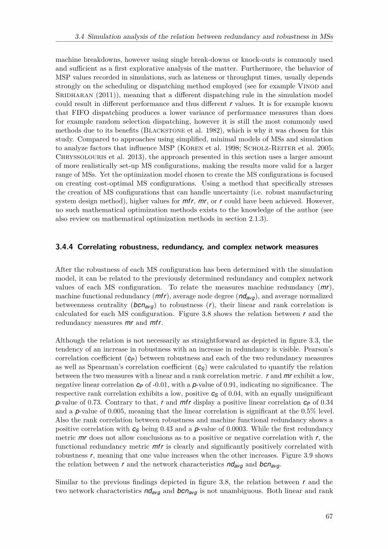
3.4 Simulation analysis of the relation between redundancy and robustness in MSs
machine breakdowns, however using single break-downs or knock-outs is commonly usedand sufficient as a first explorative analysis of the matter. Furthermore, the behavior ofMSP values recorded in simulations, such as lateness or throughput times, usually dependsstrongly on the scheduling or dispatching method employed (see for example Vinod andSridharan (2011)), meaning that a different dispatching rule in the simulation modelcould result in different performance and thus different r values. It is for example knownthat FIFO dispatching produces a lower variance of performance measures than doesfor example random selection dispatching, however it is still the most commonly usedmethods due to its benefits (Blackstone et al. 1982), which is why it was chosen for thisstudy. Compared to approaches using simplified, minimal models of MSs and simulationto analyze factors that influence MSP (Koren et al. 1998; Scholz-Reiter et al. 2005;Chryssolouris et al. 2013), the approach presented in this section uses a larger amountof more realistically set-up MS configurations, making the results more valid for a largerrange of MSs. Yet the optimization model chosen to create the MS configurations is focusedon creating cost-optimal MS configurations. Using a method that specifically stressesthe creation of MS configurations that can handle uncertainty (i.e. robust manufacturingsystem design method), higher values for mf r , mr , or r could have been achieved. However,no such mathematical optimization methods exists to the knowledge of the author (seealso review on mathematical optimization methods in section 2.1.3).
3.4.4 Correlating robustness, redundancy, and complex network measures
After the robustness of each MS configuration has been determined with the simulationmodel, it can be related to the previously determined redundancy and complex networkvalues of each MS configuration. To relate the measures machine redundancy (mr),machine functional redundancy (mf r), average node degree (ndavg), and average normalizedbetweenness centrality (bcnavg) to robustness (r), their linear and rank correlation iscalculated for each MS configuration. Figure 3.8 shows the relation between r and theredundancy measures mr and mf r .
Although the relation is not necessarily as straightforward as depicted in figure 3.3, thetendency of an increase in robustness with an increase in redundancy is visible. Pearson’scorrelation coefficient (cP) between robustness and each of the two redundancy measuresas well as Spearman’s correlation coefficient (cS) were calculated to quantify the relationbetween the two measures with a linear and a rank correlation metric. r and mr exhibit a low,negative linear correlation cP of -0.01, with a p-value of 0.91, indicating no significance. Therespective rank correlation exhibits a low, positive cS of 0.04, with an equally unsignificantp-value of 0.73. Contrary to that, r and mf r display a positive linear correlation cP of 0.34and a p-value of 0.005, meaning that the linear correlation is significant at the 0.5% level.Also the rank correlation between robustness and machine functional redundancy shows apositive correlation with cS being 0.43 and a p-value of 0.0003. While the first redundancymetric mr does not allow conclusions as to a positive or negative correlation with r , thefunctional redundancy metric mf r is clearly and significantly positively correlated withrobustness r , meaning that one value increases when the other increases. Figure 3.9 showsthe relation between r and the network characteristics ndavg and bcnavg.
Similar to the previous findings depicted in figure 3.8, the relation between r and thetwo network characteristics ndavg and bcnavg is not unambiguous. Both linear and rank
67
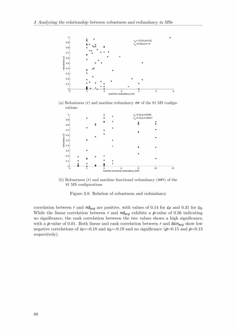
3 Analyzing the relationship between robustness and redundancy in MSs
0 1 2 3 4 5 60
0.1
0.2
0.3
0.4
0.5
0.6
0.7
0.8
0.9
1
robu
stne
ss (
r)
machinre redundancy (mr)
cP=−0.014,p=0.91
cS=0.043,p=0.73
(a) Robustness (r) and machine redundancy mr of the 81 MS configu-rations
0 2 4 6 8 10 120
0.1
0.2
0.3
0.4
0.5
0.6
0.7
0.8
0.9
1
robu
stne
ss (
r)
machine functional redundancy (mfr)
cP=0.34,p=0.0046
cS=0.43,p=0.00027
(b) Robustness (r) and machine functional redundancy (mf r) of the81 MS configurations
Figure 3.8: Relation of robustness and redundancy
correlation between r and ndavg are positive, with values of 0.14 for cP and 0.31 for cS.While the linear correlation between r and ndavg exhibits a p-value of 0.26 indicatingno significance, the rank correlation between the two values shows a high significance,with a p-value of 0.01. Both linear and rank correlation between r and bcnavg show lownegative correlations of cP=-0.18 and cS=-0.19 and no significance (p=0.15 and p=0.13respectively).
68

3.5 Summary of intermediary results
0 10 20 30 40 50 600
0.1
0.2
0.3
0.4
0.5
0.6
0.7
0.8
0.9
1
robu
stne
ss (
r)
node degree (ndavg
)
cP=0.14,p=0.26
cS=0.31,p=0.0095
(a) Robustness (r) and average node degree (ndavg) of the 81 MSconfigurations
10−5
10−4
10−3
10−2
10−1
100
0
0.1
0.2
0.3
0.4
0.5
0.6
0.7
0.8
0.9
1
robu
stne
ss (
r)
betweenness centrality (bcavg
)
cP=−0.18,p=0.15
cS=−0.19,p=0.13
(b) Robustness (r) and average normalized betweenness centrality(bcnavg) of the 81 MS configurations
Figure 3.9: Relation of robustness and complex network measures in MSs
3.5 Summary of intermediary results
In this chapter, a modeling approach for measuring redundancy in MSs was introduced,together with the assumption that an increased redundancy in a MS increases its robustness.Two redundancy measures for MSs that were suggested in the modeling approach werethen analyzed in 81 different MS configurations generated from a MSD approach usingmathematical optimization, revealing that the generated configurations exhibit a broadrange of different redundancy values. Furthermore, two measures from complex networkscience that are typically used to evaluate the robustness of complex systems, node degreeand betweenness centrality, were introduced and analyzed within the 81 MS configurations.Robustness of the MS configurations was then analyzed with a simulation study, bymeasuring the behavior of the MSP measure lateness under machine breakdowns. Theresults of the simulation study show that configurations with high and low robustnessvalues exist. Finally, the robustness values of each configuration where correlated to thesuggested redundancy and complex network measures, to investigate whether a relationshipbetween redundancy and robustness exists in MSs. The correlation analysis showed that
69

3 Analyzing the relationship between robustness and redundancy in MSs
the metrics that generally perform well for analyzing robustness in complex networks, nodedegree and betweenness centrality, show a rather weak correlation to robustness in MSs,and hence are deemed to have a low suitability as predictors for MSP robustness. However,a significant, positive linear and a significant, positive rank correlation were found betweenrobustness and the indicator machine functional redundancy. From all metrics analyzed inthis chapter as potential robustness indicators, machine functional redundancy is the onlyindicator derived from the idea of functional redundancy in biology (see section 2.3.3 andsection 3.2). As one of the key assumptions of this thesis is that the transfer of conceptsand methods from biological applications to MSs is beneficial and promising, two furthermetrics that are used to quantify system redundancy in biological contexts are introducedand applied to MSs in the following chapters 4 and 5, and their relation to MSP robustnessis analyzed. Moreover, the strong correlation between robustness and machine functionalredundancy further supports the initial assumption stated in the problem formulation ofthis thesis that robustness in MSs is raised with increasing redundancy. Machine functionalredundancy can thus serve as an indicator for robustness in MSs for example during thedesign phase of MSs, which will be further discussed in chapter 6.
70

4 Analyzing nestedness of the part-resourcesnetwork in manufacturing systems
In this chapter, the relationship between robustness and nestedness, which was introducedas an indicator for robustness of mutualistic networks in section 2.3.3, is analyzed in MSs.Similar to one of the redundancy metrics used in the previous chapter 3, the conceptof nestedness can be seen as a form of a functional redundancy. A mutualistic networkexhibits a nested structure when specialist species (show few interactions with others) onlyinteract with proper subsets of those species interacting with generalist species (show a lotof interactions with others) (Bascompte et al. 2003). This is a functional redundancy, asseveral species perform the same function as other species. Therefore metrics that measurenestedness can equally be regarded as measuring functional redundancy. Nestedness metricsare used as an indicator for system robustness, as they give an insight on how the removalof an element in the mutualistic network affects the overall network behavior with regard tobiological conservation (Atmar and Patterson 1993). In case a species disappears, thefunction of said species is not necessarily lost, as due to the nested structure of the networkthere is a high probability that another species can still perform the function of the lostspecies. A large amount of studies on ecologic networks that applied nestedness analysisrevealed general insights on robustness of mutualistic networks, showing that it is causedby the inherent redundancy of the networks (Memmott et al. 2004; Burgos et al. 2007;Bascompte and Jordano 2007). As it was pointed out in section 2.3.3, MSs share manycharacteristics with ecologic networks, for example a large network structure that favorsthe application of structural indicators or the existence of external, fluctuating influencingfactors. Therefore an application of nestedness analysis, which helped to discover strikinginsights on robustness in ecologic networks, seems favorable for MSs. Drawing an analogybetween mutualistic networks and MSs, the relationship between robustness and nestednessas a form of functional redundancy is thus analyzed within MSs in the following.
In the first section 4.1 of this chapter, the concept of nestedness is explained in more detail,and different metrics to measure it are reviewed. Subsequently, an overview on the mainfindings concerning nestedness in mutualistic and non-ecological networks is presented insection 4.2. In the following section 4.3, an analogy is drawn to model MSs as mutualisticnetworks, which enables the calculation of nestedness metrics in MSs. Nestedness is thenanalyzed in an exemplary data set of a real MS in section 4.4, showing that a generalapplication of the modeling and calculation approach is feasible. In the last section ofthis chapter, 4.5, nestedness is measured in the MS configurations created in the previouschapter 3 and linked to the robustness of the respective MSs. The results of a correlationanalysis show that a significant positive correlation between robustness and one of thenestedness metrics exists in a MS context.
71

4 Analyzing nestedness of the part-resources network in manufacturing systems
4.1 Nestedness concept and metrics3
The concept of nestedness originates from an analysis of species extinction in the RockyMountain area, where a pattern in the distribution of different montane mammal speciesamong the different mountain ranges, termed nested subset pattern or nestedness, wasidentified (Patterson 1984). Nestedness in this ecological context means that the speciesthat constitute a small fauna are proper subsets of the species that constitute richer faunas.This pattern was shown to be also present in mammalian fauna on different island groups,where smaller islands contain only a proper subset of the species found on all largerislands (Patterson and Atmar 1986). This is conceptually depicted in figure 4.1, wherea nested and a non-nested island group are shown. The circles represent biotas within theisland groups and the circle size indicates species size of the biotas. In the nested islandgroup, the species that are present in the small biota C are also present in the larger biotasB and A. In the non-nested island group, the small biota C is comprised of species whichdo not exist in all richer biotas.
A
B
C
(a) biotas are nested
C
B
A
(b) biotas are non-nested
Figure 4.1: Schematic representation of the nestedness (Patterson 1987)
When depicting a mutualistic system as a bipartite graph (see also section 2.3.3), the nestedpattern of the network is also visible in the adjacency matrix of the interaction graph.An exemplary depiction of a nested bipartite mutualistic network and its correspondingadjacency matrix is given in figure 4.2. The perfectly nested structure of the adjacencymatrix is indicated by the characteristic core of interactions in the top left corner of thematrix, with the upper half of the matrix completely filled and the lower half completelyempty. The line that separates the areas filled with ones of the matrix from the area filledwith zeros is called the extinction threshold: species are ordered such that in all habitats,the species most susceptible to extinction is the rightmost.
Already in the early works on nestedness it was argued by many authors that the nestedsubset structure of biotas has important implications for their biological conservation, i.e.their robustness to extinction (Patterson 1987; Atmar and Patterson 1993; Cutler1994). Since species in smaller biotas are not only random draws of all species in the sourcepool, but are due to the subsets also included in all the larger biotas, species might vanishfrom a small biota, but are still very likely to be present in larger biotas and thus notbecome extinct. This hypothesis was later confirmed in works such as Memmott et al.(2004), Fortuna and Bascompte (2006), or Burgos et al. (2007) (see also section 4.2).
3Parts of this section have been published in similar form in (Meyer et al. 2014).
72

4.1 Nestedness concept and metrics
A
C III
II
I
B
IV
species habitats
D
(a) exemplary nested mutualistic network (bipar-tite graph)
A B C D
I 1 1 1 1
II 1 1 1 0
III 1 1 0 0
IV 1 0 0 0
hab
itats
species
(b) adjacency matrix for 4.2a exhibiting nestedstructure
Figure 4.2: Nested structure of the adjacency matrix of an exemplary mutualistic network
Thus nestedness, which can also be seen as a form of species or functional redundancy, isseen as an indicator for the likelihood of biological conservation (i.e. robustness) of anecologic system.
In order to evaluate the extent to which a system exhibits the characteristic of nestednessdescribed above, different metrics to measure nestedness have been suggested. The metricsused within this thesis are introduced in detail in the following. An early metric called tem-perature (T ) was initially introduced by Atmar and Patterson (1993) to measure theorder or disorder in the distribution of species in fragmented habitats. T is calculatedbased on the adjacency matrix of a bipartite graph of the mutualistic network, which isalso referred to as presence-absence matrix of species and their habitats, as an entry of onein the matrix marks a species presence in a habitat and an entry of zero marks a speciesabsence in a habitat. An example of a presence-absence matrix from an observed ecologicalsystem is given in figure 4.3a. Here, the observed data from ecological systems is notordered, and the nested pattern is not immediately visible. To see the nested pattern, rowsand columns need to be rearranged from highest to lowest value respectively, as done infigure 4.3b. In the approach of Atmar and Patterson (1993) to calculate T , this processis referred to as packing or shuffling of the presence-absence matrix, and is done by analgorithm developed by the authors. After the observed incidence matrix has been packed,T is calculated based on how likely the occurrence or absence of an entry in the left orright part of the extinction threshold is. The absence of a matrix element in the area abovethe threshold or the presence of a matrix element below the threshold are unexpected in ascenario of complete nestedness. The unexpectedness of such an element depends on howfar it is away from the threshold, thus unexpectedness ui j is calculated as
ui j =(
di j
Di j
)2
(4.1)
where Di j is the length of a full line with a slope of −1 running through the jth speciesin the ith habitat and where di j is the distance from the jth species in the ith habitat tothe threshold along this line (Atmar and Patterson 1993; Rodriguez-Girones andSantamaria 2006). This is also conceptually depicted in 4.4, where point X represents anunexpected presence of a species, and point Y represents the point where a line with theslope of -1 that runs through point X meets the threshold. The total unexpectedness (U)
73

4 Analyzing nestedness of the part-resources network in manufacturing systems
n1 n2 n3 n4
m1 0 0 0 1
m2 1 1 1 1
m3 0 1 1 1
m4 0 1 0 1
hab
itats
species
1
4
3
2
1 3 2 4
(a) observed presence-absence matrix
n1 n2 n3 n4
m1 1 1 1 1
m2 1 1 1 0
m3 1 1 0 0
m4 1 0 0 0
ha
bit
ats
species
4
3
2
1
4 3 2 1
most
stable
most
tenuous
most hospitable
least hospitable
(b) maximally packed matrix for 4.3a
Figure 4.3: Shuffling of an observed presence-absence matrix, modified from (Atmar andPatterson 1993)
of the entire matrix is then calculated as
U =1
m · n∑
i
∑j
ui j (4.2)
where m is the total number of habitats and n is the total number of species (Atmar andPatterson 1993).
n species
m isla
nds
dij
Dij
A
B
Figure 4.4: Measuring unexpectedness of point X in an exemplary matrix, modifiedfrom (Atmar and Patterson 1993) and (Rodriguez-Girones and Santa-maria 2006)
This measure is then normalized to receive the nestedness metric temperature (T ), which iscalculated as the ratio between the total unexpectedness of species extinction (U) and themaximum unexpectedness (Umax), which is a constant derived from a matrix of maximumunexpectedness (Atmar and Patterson 1993).
T =100
Umax· U (4.3)
74

4.1 Nestedness concept and metrics
T can range between 0 and 100◦, with values around 0◦ indicating perfect nestednessand values close to 100◦ indicating completely random matrices. Note that the presence-incidence matrix does not need to be square for this measure to be applicable. For thecalculation of the temperature as presented here, Atmar and Patterson (1993) createda freely available software called Nestedness Temperature Calculator (NTC).
Over the years, several extensions and variations of this initially proposed nestednessmeasure have been established (Guimaraes Jr. and Guimaraes 2006; Rodriguez-Girones and Santamaria 2006; Almeida-Neto et al. 2008; Araujo et al. 2010),of which the most frequently used ones are introduced in the following. Guimaraes Jr.and Guimaraes (2006) developed an improved algorithm to calculate T , which allowscalculating the temperature in several matrices at the same time. They implemented thisalgorithm in their freely available software called Aninhado. In Rodriguez-Girones andSantamaria (2006), a new algorithm for the shuffling of the incidence matrix is developedand implemented into a software called binary nestedness temperature calculator (BIN-MATNEST). It outperforms the initially proposed algorithm by Atmar and Patterson(1993) for specific matrix layouts (e.g. checkerboard patterned matrices). Almeida-Netoet al. (2008) introduced a new metric to measure nestedness, called the nestedness metricbased on overlap and decreasing fill (NODF). While T is calculated based on the distancesof an expected or unexpected occurrence of a fill in the matrix from an isocline, NODF iscalculated using a pairwise comparison of the fills in the matrix rows and columns and therows and column overlap. In comparison to T , NODF is less affected by species number(number of rows/ columns in the matrix) (Almeida-Neto et al. 2008), thus it moreaccurately depicts the conceptual idea of nestedness and has become increasingly popularamong ecologists in the recent past. As both measures, T and NODF , will be used inthe following section, the calculation of NODF is introduced in detail in the upcomingparagraph.
NODF is, as T , calculated from an incidence matrix with m rows and n columns. Rowsthat are further "up" (i) are compared to rows "below" (j), and columns that are locatedfurther "left" (k) are compared to columns further to the "right" (l) (Almeida-Neto et al.2008). The decreasing fill (DF ) does a pairwise comparison whether a row that is furtherup or a column that is further left has more entries of 1’s than a row further down or acolumn further to the right. The decreasing fill in a pair of rows i and j (DFi j) is equalto 100 if the marginal total (MT ), which is the sum of 1’s in a row or column, in MTj issmaller than in MTi . If the sum of 1’s in MTj is larger or equal to MTi , then DFi j is equal to0. The same holds for the pairwise comparison of the columns: DFkl is 100 if MTl < MTk
and 0 if MTl ≥ MTk . The paired overlap (PO) compares for a pair of rows or columnshow many 1’s in a row or column are located at the same location than in the other rowor column of the pair (in percent). The paired overlap of a pair of rows i and j (POi j) isthe percentage of 1’s in row j that are located at the identical column position in row i.Likewise, the paired overlap of a pair of columns k and l (POkl) is the percentage of 1’s incolumn l that are located at the identical row position in column k . The degree of pairednestedness (Npaired), either for a pair of rows or columns, will take the value 0 if the DFof this pair is equal to 0. If the DF of the pair is 100, Npaired will take the value of PO.The measure for nestedness for the whole matrix (NODF) is then calculated as the sumof all Npaired (of rows and columns), averaged by number of rows (m) and columns (n) asshown in equation 4.4. In figure 4.5, the calculation of NODF for an exemplary matrix is
75
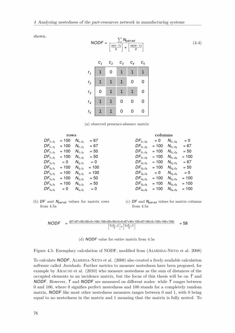
4 Analyzing nestedness of the part-resources network in manufacturing systems
shown.NODF =
∑Npaired[
n(n−1)2
]+[
m(m−1)2
] (4.4)
c1 c2 c3 c4 c5
r1 1 0 1 1 1
r2 1 1 1 0 0
r3 0 1 1 1 0
r4 1 1 0 0 0
r5 1 1 0 0 0
(a) observed presence-absence matrix
rowsDFr1,r2 = 100 Nr1,r2 = 67DFr1,r3 = 100 Nr1,r3 = 67DFr1,r4 = 100 Nr1,r4 = 50DFr1,r5 = 100 Nr1,r5 = 50DFr2,r3 = 0 Nr2,r3 = 0DFr2,r4 = 100 Nr2,r4 = 100DFr2,r5 = 100 Nr2,r5 = 100DFr3,r4 = 100 Nr3,r4 = 50DFr3,r5 = 100 Nr3,r5 = 50DFr4,r5 = 0 Nr4,r5 = 0
(b) DF and Npaired values for matrix rowsfrom 4.5a
columnsDFc1,c2 = 0 Nc1,c2 = 0DFc1,c3 = 100 Nc1,c3 = 67DFc1,c4 = 100 Nc1,c4 = 50DFc1,c5 = 100 Nc1,c5 = 100DFc2,c3 = 100 Nc2,c3 = 67DFc2,c4 = 100 Nc2,c4 = 50DFc2,c5 = 0 Nc2,c5 = 0DFc3,c4 = 100 Nc3,c4 = 100DFc3,c5 = 100 Nc3,c5 = 100DFc4,c5 = 100 Nc4,c5 = 100
(c) DF and Npaired values for matrix columnsfrom 4.5a
NODF = (67+67+50+50+0+100+100+50+50+0+0+67+50+100+67+50+0+100+100+100)[5∗(5−1)
2
]+[
5∗(5−1)2
] = 58
(d) NODF value for entire matrix from 4.5a
Figure 4.5: Exemplary calculation of NODF, modified from (Almeida-Neto et al. 2008)
To calculate NODF , Almeida-Neto et al. (2008) also created a freely available calculationsoftware called Aninhado. Further metrics to measure nestedness have been proposed, forexample by Araujo et al. (2010) who measure nestedness as the sum of distances of theoccupied elements in an incidence matrix, but the focus of this thesis will be on T andNODF . However, T and NODF are measured on different scales: while T ranges between0 and 100, where 0 signifies perfect nestedness and 100 stands for a completely randommatrix, NODF like most other nestedness measures ranges between 0 and 1, with 0 beingequal to no nestedness in the matrix and 1 meaning that the matrix is fully nested. To
76

4.2 Application of nestedness analysis in ecological and non-ecological systems
make both measures comparable, the normalized Tn will be used in the following analysis,which is calculated as
Tn =(100− T )
100(4.5)
The general procedure of a nestedness analysis first requires that a metric to quantify thepattern of nestedness in a matrix is calculated, and then the metrics are compared with anappropriate null model or randomization test to assess the statistical significance of themetric (Ulrich et al. 2009).
4.2 Application of nestedness analysis in ecological andnon-ecological systems4
Nestedness has been extensively analyzed in various ecological systems, using a variety ofdifferent metrics. In a large-scale study by Bascompte et al. (2003), 52 different plant-animal mutualistic networks were analyzed using T as a nestedness measure, and nearly all ofthe analyzed pollination or seed dispersal networks were found to be significantly nested. Itwas further shown that nestedness increases with complexity (number of interactions) of thenetwork (Bascompte et al. 2003). Guimaraes Jr. et al. (2006) analyzed four mutualisticnetworks of ants and extrafloral nectary-bearing plants also using T as a nestedenessmeasure, and found that three out of the four networks are highly nested. In Ollertonet al. (2007), it was shown that a marine mutualistic network of anemone fish and seaanemones is also strongly nested, using also T as a nestedness measure. A further studyanalyzed three mutualistic networks of cleaning symbiosis in reefs using T as a nestednessmeasures, and revealed that all investigated networks are strongly nested (GuimaraesJr. et al. 2007). Kondoh et al. (2010) analyzed nestedness in 31 trophic food webs bytransforming the usually unipartite food networks into bipartite networks. They used Tand NODF as measures for nestedness and showed that 65% of the analyzed food webswere nested. In James et al. (2012), 59 different plant-pollinator networks are studied withregard to nestedness (measured by NODF ) and it was found that the different ecologicnetworks exhibit strongly varying nestedness values, ranging from close to 0 to 0.8.
In addition to the several studies that examine the nestedness values ecologic systemsdisplay, a further stream of research is also dedicated to studying the relation of nestednessto robustness of ecologic systems. Memmott et al. (2004) studied two large mutualisticnetworks of plants and flower visitors to gain insight on their biological conservation abilities(i.e. their robustness to extinction of either plants or flowers). For this they simulatedspecies extinction by removing pollinators from the network using three different algorithm,and analyzed which and how many plants were left non-pollinated after removal. Theirresults show that both mutualistic systems studied are relatively robust against removal ofpollinators, and they conclude that the robustness of mutualistic networks "derives fromredundancy in pollinators per plant and from nested topology of the networks" (Memmottet al. 2004). In the approach by Fortuna and Bascompte (2006), the robustness oftwo real ecologic networks is compared to randomized versions of the real networks. Theauthors find that the real networks are more robust to higher destruction levels: although
4Parts of this section have been published in similar form in (Meyer et al. 2014).
77

4 Analyzing nestedness of the part-resources network in manufacturing systems
species start to decay sooner when habitat is lost in the real networks, the thresholdat which all species go extinct is significantly higher in the real networks than in therandomized networks. They argue that this behavior stems from the nested structure ofthe real networks, where the dense core of generalist animals and plants "is very robust tohabitat loss" (Fortuna and Bascompte 2006). Burgos et al. (2007) measure robustnessof a mutualistic system, similar to Memmott et al. (2004), as the tolerance to the removalof species. They analyze several different mutualistic networks and conclude that a "closepositive relationship" (Burgos et al. 2007) exists between nestedness and robustness inmutualistic networks.
A variety of different real-world and man-made networks have also been found to exhibitnested characteristics. Saavedra et al. (2009) analyzed ecological and organizationalnetworks and found that a network of manufacturer-contractor interactions exhibits similar,i.e. nested, structural patterns as mutualistic plant-animal pollination networks. Theanalysis of nested structures has further been applied to data of countries and their tradeproducts by Ermann and Shepelyansky (2013), who discovered that the network ofcountries and their trade products exhibits analogous features to plant-pollinators networks,i.e. they are highly nested. It has also been shown for two large-scale automotive supplychains (Toyota and Ford) that they exhibit highly nested patterns in their supplier-productrelations (Kito and Ueda 2014). Similarly, Brintrup et al. (2015) also discover nestedpatterns in data on supplier-product and supplier-manufacturer relations from automotivesupply chains.
However, the concept of nestedness and its measures are also discussed critically by severalauthors, for example by James et al. (2012) or Staniczenko et al. (2013), who claimthat the largest drawback of most nestedness measures is that they ignore interactionfrequencies between the two bipartite types of nodes that are connected in the network.This means all links are always regarded as equally important, even if for example some ofthe plants or pollinators exist in significantly larger volumes than others.
4.3 Modeling manufacturing systems as mutualistic networks5
Similar to the question of biological conservation and system robustness in ecologicalsystems, MSs need to be designed in a way that their performance stays robust againstdifferent fluctuations and disturbances (see section 2.1.4). In ecological systems, nestednessis used as an indicator for system robustness, as it gives an insight on how the removal ofhabitats or the extinction of species affects the system. To apply the concept of nestednessand its measures to MSs, analogies between the previously introduced ecological systems(see section 2.3.3) and MSs are drawn in this section. The bipartite, mutualistic networksthat are subject to nestedness analysis in ecology usually consist of relations between plantsand their seed dispersers or between habitats and the species that live in them (exemplaryconceptual depiction in figure 4.6a). To measure nestedness in a manufacturing context,relations between resources and the parts that are processed on the resources are depictedas a bipartite network, where nodes are either resources or parts and the links betweenthe nodes signify that a part is processed by the linked resource (exemplary conceptualdepiction in figure 4.6b). A removal of a species (species extinction) is then analogous
5Parts of this section have been published in similar form in (Meyer et al. 2014).
78

4.3 Modeling manufacturing systems as mutualistic networks
to the removal of a certain part (e.g., if a part/ product is removed from the productportfolio), while the destruction of a habitat is analogous to the removal of a resource (e.g.,machine breakdown). In such a bipartite depiction, each MS exhibits a specific nestednessvalue.
A
C
III
II
I
B
IV
species habitats
(a) exemplary bipartite species-habitat graph
A
C
III
II
I
B
IV
parts resources
IV
(b) exemplary bipartite part-resource graph
Figure 4.6: Exemplary depictions of bipartite ecological, mutualistic network and bipartitemanufacturing network
The data necessary to calculate nestedness in the parts-resources network is either availablefrom the design or process planning department or can easily be derived from the operationsor route sheets of the parts or final products (see section 2.1.1). It can also be derivedfrom feedback data, which can be obtained from the manufacturing execution system ofa MS. An exemplary derivation of a parts-resources matrix (analogous to the species -habitat matrix) from a route sheet of exemplary parts that together form a product isdepicted in figure 4.7. Note that if more then one resource per part is given in the routesheet (figure 4.7a), these are alternative resources, meaning that the part can be treatedon either of them.
A
D
part product
C
raw material
E
F G
B
processing and/ or assembly
part step process resource
A 1 assembly I
B 1 drilling III, IV, V
B 2 sanding VI, VII
C 1 welding II
D 1 drilling III, IV, V
D 2 sanding VI, VII
E 1 assembly I
F 1 drilling III, IV, V
G 1 grinding VIII
(a) route sheet for exemplary parts
A B1 B2 C D1 D2 E F G
I 1 0 0 0 0 0 1 0 0
II 0 0 0 1 0 0 0 0 0
III 0 1 0 0 1 0 0 1 0
IV 0 1 0 0 1 0 0 1 0
V 0 1 0 0 1 0 0 1 0
VI 0 0 1 0 0 1 0 0 0
VII 0 0 1 0 0 1 0 0 0
VIII 0 0 0 0 0 0 0 0 1
res
ou
rce
s
parts
(b) the part-resource matrix derived from 4.7a
Figure 4.7: Deriving the part-resource matrix from an exemplary route sheet, modifiedfrom (Meyer et al. 2014)
79

4 Analyzing nestedness of the part-resources network in manufacturing systems
In a bipartite parts-resources network, a change in parts or products (e.g., the discontinua-tion of a product), directly affects the composition of the network and matrix representation,meaning that it will have lesser columns and thus also a different nestedness value. Likewise,the removal of a resource also results in a change in the amount of columns of the matrix.Similar to analyses in ecology, conclusions can be drawn from this parts-resources matrixas to whether certain parts have alternative routes through the system. By linking thisnestedness value to the robustness of MSP (as defined in section 3.1), it can be analyzedwhether nestedness can also be used as a suitable predictor for MSP robustness. Theanalogy thus allows to evaluate, how performance robustness is affected by the structuralaspects, i.e. parts and the corresponding resources, of the MS. The idea of analyzing theeffect of changes in the part-resources relations on the manufacturing performance is similarto recent investigations of the blocking effect that the product structure can impose on themanufacturing process flow (Martínez-Olvera 2012). Martínez-Olvera (2012) arguesthat as products are made up of various parts, conflicts in the use of resources can arise asdifferent parts might need to undergo the same operations on the same resources. Thisnotation is also similar to the part-machine matrices used in group technology or design ofcellular MSs, which aim at grouping machines according to the process combinations thatoccur in families of parts (Askin 2013). However, in this thesis, the part-resource matrixis used for a different purpose, namely to study the performance robustness of the systemin relation to operational redundancy.
4.4 Application of nestedness analysis to a case studymanufacturing system6
4.4.1 Description of the analyzed system
In this section, the structure of the part-resource network in a real job shop environmentis analyzed with regards to nested characteristics. The part-resource network is derivedfrom an actual manufacturing facility, which is organized as a job shop and produceslarge press-tools. The production process includes the manufacturing of different metalcomponents, which are later assembled into a press-tool. The assembly step is not part ofthe analysis of the network of parts and machines. The job shop consists of 32 machines,which are grouped according to the operation that they are able to perform. Figure 4.8shows the number of machines per machine group as well as the material flows between themachines. Similar to ecological systems, there is a certain amount of redundancy inherentin the manufacturing system, as for the treatment of some of the parts, several resourcesare available. 241 unique parts were identified from 7 months of production feedback data,which was collected from the job shop’s production planning and control software. With32 machines as resources, this results in a 241 x 32 parts-resources matrix.
6Parts of this section have been published in similar form in (Meyer et al. 2014).
80

4.4 Application of nestedness analysis to a case study manufacturing system
source drain
cutting
portal
milling turning
round
grinding
flat
grinding
medium
milling
small milling
eroding
machine machine group material flow
Figure 4.8: Machines and material flows in the analyzed job shop, modified from (Meyeret al. 2014)
4.4.2 Nestedness calculation and discussion of results
The previously introduced nestedness measures Tn (see equation 4.5) and NODF (seeequation 4.4) are used to calculate nestedness of the parts-resources matrix. To calculateTn of the parts-resources matrix, several free programs are available, for example theNestedness Temperature Calculator by Atmar and Patterson (1993), the Binmatnestcalculator by Rodriguez-Girones and Santamaria (2006), or the Aninhado calculatorby Guimaraes Jr. and Guimaraes (2006). The difference between these calculatorsis that the resulting temperature values usually differ from each other, as Binmatnestand Aninhado use slightly improved algorithms to generate the nested matrix, thus theyrepresent extensions of the Nestedness Temperature Calculator. For this case study, theAninhado calculator is chosen, as it is also able to calculate NODF . The calculationresults in a Tn value of 0.77 and a NODF value of 0.00 for the parts-resources matrix.The relatively high Tn value indicates that the analyzed matrix is nested. In mutualisticnetworks, the term highly, at which networks are considered to be highly nested, rangesbetween 0.75 and 1 (Bascompte et al. 2003). As Tn of the part-resources matrix is withinthis range, the network can be described as highly nested. However, the low NODF valueindicates that the matrix is not nested at all. The fact that the results for both metrics differso strongly is not surprising for the analyzed network: it is strongly compartmented and hasa low fill (percentage of 1’s in the matrix), which can be seen in figure 4.9, and it was shownby Almeida-Neto et al. (2008) that NODF yields values of zero for such compartmentedmatrices or matrices with beta-diversity. However, NODF will still be analyzed in thefollowing section as it has been shown to be superior to Tn in many ecological contexts(see for example Ulrich et al. (2009)). Figure 4.9 is a plot of the analyzed matrix aftershuffling which clearly shows that the matrix is compartmented and also minimally filled(11%).
81

4 Analyzing nestedness of the part-resources network in manufacturing systems
resources
part
s
10 20 30
50
100
150
200
Figure 4.9: Nested matrix of the parts-resources matrix of the analyzed company, modifiedfrom (Meyer et al. 2014)
Similar to ecological systems, the nested matrix of the analyzed parts-resources networkexhibits a central core of machines in the top left corner. As opposed to the findings inecological systems, a completely nested structure with nestedness values close to one willmost likely seldom be found in a parts-resources network, as this would require some ofthe resources in the network to be able to conduct all manufacturing processes present inthe system (comparable to the most stable species in the ecological systems, which canbe found in all habitats). This is only possible if the process variety within the MS isnot high and if some of the machines are flexible machining centers that can conduct allpossible manufacturing processes. As this case study has shown that the general conceptand calculation of nestedness are applicable to real manufacturing data, the followingsection analyzes the general relation between nestedness as a redundancy indicator andMSP robustness in MSs, using the 81 MS configurations created in chapter 3.
4.5 Application of nestedness analysis to the test manufacturingsystem configurations
4.5.1 Nestedness calculation and discussion of results
To study the general relationship of robustness and nestedness in MSs, the 81 MS configu-rations that were established in the previous section 3.4 are used in this section. In a firststep, the two different nestedness measures used in the previous section 4.4 (Tn and NODF )are calculated for each of the 81 MS configurations. For the calculation of Tn and NODF
82

4.5 Application of nestedness analysis to the test manufacturing system configurations
in each configuration, the freely available Matlab library BiMat was used. Contrary to thepreviously used Aninhado calculator which can only calculate nestedness in one matrix ata time, it is possible to analyze several matrices at once with BiMat. Within BiMat, Tn
is calculated using the algorithm suggested by (Atmar and Patterson 1993), whereasNODF is calculated using the algorithm by (Almeida-Neto et al. 2008). Figure 4.10compares both nestedness measures per MS configuration. The resulting nestedness valuesfor each configuration can be found in Appendix D.
0 10 20 30 40 50 60 70 800
0.1
0.2
0.3
0.4
0.5
0.6
0.7
0.8
0.9
1
nest
edne
ss (
Tn)
MS configuration
(a) Tn values for the 81 MS configurations
0 10 20 30 40 50 60 70 800
0.1
0.2
0.3
0.4
0.5
0.6
0.7
nest
edne
ss (
NO
DF
)
MS configuration
(b) NODF values for the 81 MS configurations
Figure 4.10: Nestedness values of the 81 MS configurations
Similar to the results for the redundancy metrics mr and mf r in section 3.4.2, MS configu-rations with high and low values for both Tn and NODF exist. This is in coherence withfindings from ecological networks, which also exhibit a wide range of different nestednessvalues between 0 and 1 (see for example (James et al. 2012)). The average of Tn over allMS configurations lies at 0.57 which is a lot higher than the average of 0.31 for NODF overall MS configurations. Values for NODF also vary slightly stronger (standard deviation of0.2) than those for Tn (standard deviation of 0.13). This can easily be explained with themany values of 0.0 that NODF takes for 17 MS configurations. This behavior is also inline with what was found in the analysis of the case study of real MS system data, where
83

4 Analyzing nestedness of the part-resources network in manufacturing systems
Tn indicated a rather strong nestedness (0.75) while NODF indicated no nestedness (0.0).The fact that both metrics can differ strongly for the same network and that NODF evenindicates non-existing nestedness while Tn shows rather strong nestedness is also commonin mutualistic networks, due to the substantially different measurement logic both metricsuse (as explained in section 4.1). Overall, both measures do not indicate as high nestednessmeasures (on average) as in the analysis for mutualistic networks (the average nestedness of52 mutualistic networks in Bascompte et al. (2003) lies at 0.82). Thus it can be concludedthat MS configurations in general are not as strongly nested as mutualistic networks. Anexplanation for this was already given in the small case study of real manufacturing data:a completely nested structure with nestedness values close to one will most likely seldombe found in a parts-resources network of a MS, as this would require some of the resourcesin the network to be able to conduct all manufacturing processes present in the system.
4.5.2 Correlating robustness and nestedness
In order to analyze the relation between robustness and nestedness in MS, the nestednessvalues are correlated to the robustness values of the 65 MS configurations, which werecalculated in section 3.1. Figure 4.11 shows the relation between robustness (r) and thenestedness values Tn and NODF in the 65 MS configurations.
The linear correlation between r and Tn is positive, with an extremely low Pearson’scorrelation coefficient of cP = 0.07 and a p-value of 0.5, indicating no significant correlation.The rank correlation between r and NODF is also positive, with a rather weak correlationcoefficient of cr = 0.22 at a significant p-value of 0.05. From this it is concluded that with ahigher NODF value, robustness of the MSP measure lateness against machine breakdownsalso increases slightly. The reason why the scatter plots show the values for Tn more in theright and for NODF more to the left side of the axis lies in the different values ranges forTn and NODF , explained also in the previous figure 4.10.
84

4.6 Summary of intermediary results
0 0.1 0.2 0.3 0.4 0.5 0.6 0.7 0.8 0.9 10
0.1
0.2
0.3
0.4
0.5
0.6
0.7
0.8
0.9
1
robu
stne
ss (
r)
Tn per MS configuration
cP=−0.047,p=0.71
cS=−0.067,p=0.59
(a) Robustness (r) and nestedness (Tn) of the 81 MS configurations
0 0.1 0.2 0.3 0.4 0.5 0.6 0.7 0.8 0.9 10
0.1
0.2
0.3
0.4
0.5
0.6
0.7
0.8
0.9
1
robu
stne
ss (
r)
NODF per MS configuration
cP=0.29,p=0.016
cS=0.31,p=0.0095
(b) Robustness (r) and nestedness (NODF ) of the 81 MS configurations
Figure 4.11: Relation of robustness and nestedness
4.6 Summary of intermediary results
The aim of this chapter was to analyze the relationship between nestedness, a robustnessindicator used in the analysis of ecologic systems, and robustness of MS performance. Tocalculate nestedness in MSs, an approach for modeling MSs as mutualistic networks wasintroduced first. Nestedness was then calculated both in an exemplary real world casestudy data set of a job shop MS, and in the 81 MS configurations generated in section 3.4.2,showing the general applicability of the concept to MS data. The calculation of nestednessfurther revealed that both the case study data set and the MS configurations exhibit highnestedness values for Tn and NODF , two classical nestedness measures that were introducedin this chapter. However, the average nestedness values found for the MSs are significantlylower than those usually found in mutualistic networks (see for example Bascompte et al.(2003)). As discussed in detail in section 4.4.2, this might be the case since true generalists,i.e. machines that can conduct every manufacturing step found in a job shop, usually donot exist in a manufacturing context. Thus a completely nested matrix is highly unlikely
85

4 Analyzing nestedness of the part-resources network in manufacturing systems
to exist in the case of a parts-resource network of a MS. Moreover, the correlations of bothnestedness measures Tn and NODF to robustness r of MSs are rather weak and only oneof them is significant. Consequently, it is concluded that for the analyzed configurations,nestedness does not serve as an equally good indicator for robustness in MSs as it does inmutualistic networks. Compared to the findings from the previous chapter, the correlationfound between machine functional redundancy (mf r) and robustness (r) of MSs exhibiteda strikingly larger significance.
86

5 Analyzing elementary flux modes in theresources-material flow network inmanufacturing systems
In the fifth chapter, EFMs, which were introduced as a robustness indicator in metabolicnetworks in section 2.3.3, are analyzed in MSs. Similar to one of the redundancy metricsused in chapter 3 and the nestedness metrics used in chapter 4, EFMs can be seen as aform of functional redundancy. An EFM is a non-decomposable chemical reaction path in ametabolic network that allows for autonomous function of the underlying organism (Schus-ter and Hilgetag 1994). While EFMs can be defined for arbitrary (categories of) startand end points, they are mostly used to analyze paths from nutrients (i.e. external resources)to biomass components (i.e. final products) (Schuster and Hilgetag 1994; Schusteret al. 1999). If several paths in a metabolic network lead to the production of the samecomponent, this is also referred to as pathway redundancy (Papin et al. 2002; Price et al.2002). In systems biology, EFMs are used for example as an indicator for robustness ofa metabolic network, as it was shown that the number of EFMs in a metabolic networkdirectly relates to the robustness of the network against gene deletion (Stelling et al.2002; Wilhelm et al. 2004). Moreover, EFMs were shown to be a better predictor forsystem robustness in metabolic networks than for example standard metrics from complexnetworks science (Stelling et al. 2002). As explained in section 2.3.3, metabolic systemsshare a lot of strong commonalities with MSs, such as the internal and external fluctuationsboth systems are faced with (see also figure 2.18). An application of EFMs, which areused to relate network structure to function in metabolic networks, is therefore suitableto link the purely structural aspects of redundancy in MSs to a system function such asrobustness of a performance measure. Similar to the previous chapter on nestedness inMSs, the relation between the structural indicator EFMs and robustness in MSs is analyzedin the following.
To transfer EFM analysis to a MS context, a description of how EFMs are calculated in asystems biology context is given as a first step in section 5.1. It is further explained therehow insights on cell metabolism were gained using EFM analysis and in which aspects thismethod has been shown to be superior to similar approaches. As already introduced insection 2.3.3, striking structural similarities exist between manufacturing and metabolicsystems. Building on these similarities, an analogy is drawn how a MS network can bemodeled as a metabolic network to be able to calculate EFMs in MSs in section 5.2. Inorder to show the applicability of EFM analysis to a real world MSs, EFMs are calculatedfor an exemplary case study data set of a real world MS in section 5.3. Within thiscase study, EFMs are compared to a classical measure for machine significance from amanufacturing context and to two classical measures from complex-network science. Itis shown that EFMs can be used as an equally good or even better predictor for MSsrobustness of the performance measures lateness than the other analyzed measures. As the
87

5 Analyzing elementary flux modes in the resources-material flow network in MSs
case study indicates that a relation between EFMs and MS robustness exists, this relationis analyzed on a broader level in section 5.4, where the EFMs of the MS configurationscreated in section 3.4 are first calculated, and then correlated to the robustness of therespective MS configurations.
5.1 Elementary flux mode analysis in metabolic networks7
As introduced in section 2.3.3, a metabolic system is the complete set of chemical reactionswithin a cell, and is referred to as a metabolic network when depicted in a graph-theoreticalrepresentation (Palsson 2015). An exemplary metabolic reaction network is depictedin figure 5.1a. A chemical reaction between enzymes and metabolites usually containsthe metabolites and their concentrations, given as stoichiometric coefficients in chemicalreaction equations (Palsson 2015). As a metabolic system consists of several chemicalreactions taking place, an entire system of chemical reaction equations exists per metabolicsystems. These chemical reactions - including the stoichiometric coefficients - of a metabolicnetwork can be depicted as a stoichiometric matrix (Palsson 2015). The stoichiometricmatrix of a metabolic network is the data basis for EFM calculation. Every column of astoichiometric matrix corresponds to a reaction and every row to a metabolite of a metabolicreaction network. The stoichiometric coefficients entered in the matrix are integers. Thisis also depicted in figure 5.1b, which shows the stoichiometric matrix corresponding to theexemplary metabolic reaction network in figure 5.1a.
ext1
r1
r2
r3
r4
m1
ext3
r7
r6 ext2
r5
r = reaction m = metabolite ext = external metabolite
m2
m3
m4
(a) exemplary metabolic reaction network
r1 r2 r3 r4 r5 r6 r7
m1 1 −1 −1 0 0 0 0m2 0 1 1 −1 0 0 0m3 0 0 0 0 1 −1 0m4 0 0 0 1 0 1 −1
(b) stoichiometric matrix for 5.1a
Figure 5.1: Metabolic network modeling, modified from (Meyer et al. 2016)
As mentioned in the beginning of this chapter, EFMs of a metabolic network are the setof vectors that form the smallest sub-network of the original metabolic network whichstill allows a metabolic network to function in steady state (Schuster and Hilgetag1994; Klamt and Stelling 2003; Papin et al. 2003). They can be defined for arbitrarystart (corresponds to external metabolites ext1 and ext2 in figure 5.1a) and end points(corresponds to external metabolite ext3 in figure 5.1a) in a metabolic system, whichare mostly chosen to be paths from specific nutrients (inputs) to biomass components(outputs) (Schuster and Hilgetag 1994; Schuster et al. 1999). As shown in figure 5.2,an EFM is defined by a vector, which is composed of elements that each describe the net
7Parts of this section have been published in similar form in (Meyer et al. 2016).
88
5.1 Elementary flux mode analysis in metabolic networks
rate of the corresponding reaction from the stoichiometric matrix (i.e. such a vector orEFM is a flux distribution) (Klamt and Stelling 2003).
r = reaction EFM = elementary flux mode
EFM1 = EFM2 = EFM3=
0
0
0
0
1
1
1
1
0
1
1
0
0
1
1
1
0
1
0
0
1
r1
r2 r4
r1
r3
r4
r6
r5 r7 r7
r7
Figure 5.2: EFMs of the metabolic reaction network shown in figure 5.1a, modifiedfrom (Meyer et al. 2016)
A pathway through the metabolic system is thus identified by the utilized chemical reactions.One of the first mathematical definitions of EFMs, which has been given by Schusterand Hilgetag (1994), states that, in case all fluxes have fixed signs, all EFMs of ametabolic network are given by the set of generating vectors of a convex polyhedral cone.Such polyhedral cones are a well-studied convex set in computational geometry, thuscalculating the EFMs of a metabolic network can be said to be equivalent to extreme rayenumeration of polyhedral cones (Terzer and Stelling 2008). Different algorithms forcomputing the generating vectors of convex polyhedral cones were then suggested, forexample by Schuster and Hilgetag (1994) or Terzer and Stelling (2008), and manyof them were implemented into software that is freely available for computation of EFMs.
In systems biology, EFMs are used to investigate the stoichiometry and structural propertiesof metabolic networks (Schuster et al. 1999; Schuster et al. 2000). Additionally, theyhave been extraordinarily successful, compared to other structural network measures, as apredictor for system robustness of metabolic systems (Stelling et al. 2002; Wilhelmet al. 2004; Behre et al. 2008), specifically for robustness against mutations. Theprediction of lethal mutations (i.e. mutations that render the metabolic system nonviable)in systems biology had previously been addressed using a huge range of predictors derivedfrom complex network science. Jeong et al. (2000) modeled metabolic systems as networksin which the degree of a node is a measure of the node’s importance and the broad degreedistribution implements a high robustness against random failures (at the expense of ahigh vulnerability of targeted attacks against the high-degree nodes). In Wunderlichand Mirny (2006), the change of synthetic accessibility (which is a variant of the networkdiameter) has been employed for this task. Comparing their synthetic accessibility measureto other topology-based characteristics, such as node degree, graph diameter, or nodeusage, they show that these classical measures fail as a predictor for lethal mutations. Inaccordance with this, it was shown by Stelling et al. (2002) that the graph theoreticalmeasure of the network diameter (defined as the average minimal path length between anytwo nodes), which is typically used as an indicator whether a network is invariant to randomremoval of nodes, did not indicate functionality of the metabolism under study, while thenumber of EFMs clearly did. This questions of robustness against is lethal mutations is
89
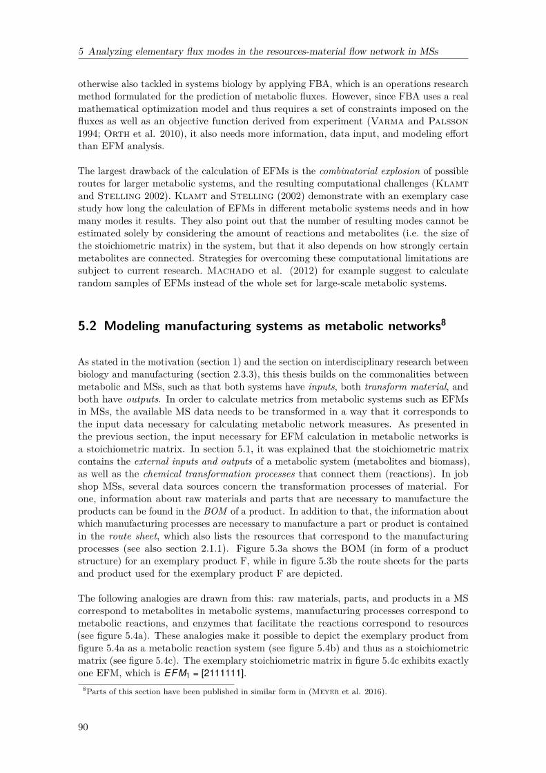
5 Analyzing elementary flux modes in the resources-material flow network in MSs
otherwise also tackled in systems biology by applying FBA, which is an operations researchmethod formulated for the prediction of metabolic fluxes. However, since FBA uses a realmathematical optimization model and thus requires a set of constraints imposed on thefluxes as well as an objective function derived from experiment (Varma and Palsson1994; Orth et al. 2010), it also needs more information, data input, and modeling effortthan EFM analysis.
The largest drawback of the calculation of EFMs is the combinatorial explosion of possibleroutes for larger metabolic systems, and the resulting computational challenges (Klamtand Stelling 2002). Klamt and Stelling (2002) demonstrate with an exemplary casestudy how long the calculation of EFMs in different metabolic systems needs and in howmany modes it results. They also point out that the number of resulting modes cannot beestimated solely by considering the amount of reactions and metabolites (i.e. the size ofthe stoichiometric matrix) in the system, but that it also depends on how strongly certainmetabolites are connected. Strategies for overcoming these computational limitations aresubject to current research. Machado et al. (2012) for example suggest to calculaterandom samples of EFMs instead of the whole set for large-scale metabolic systems.
5.2 Modeling manufacturing systems as metabolic networks8
As stated in the motivation (section 1) and the section on interdisciplinary research betweenbiology and manufacturing (section 2.3.3), this thesis builds on the commonalities betweenmetabolic and MSs, such as that both systems have inputs, both transform material, andboth have outputs. In order to calculate metrics from metabolic systems such as EFMsin MSs, the available MS data needs to be transformed in a way that it corresponds tothe input data necessary for calculating metabolic network measures. As presented inthe previous section, the input necessary for EFM calculation in metabolic networks isa stoichiometric matrix. In section 5.1, it was explained that the stoichiometric matrixcontains the external inputs and outputs of a metabolic system (metabolites and biomass),as well as the chemical transformation processes that connect them (reactions). In jobshop MSs, several data sources concern the transformation processes of material. Forone, information about raw materials and parts that are necessary to manufacture theproducts can be found in the BOM of a product. In addition to that, the information aboutwhich manufacturing processes are necessary to manufacture a part or product is containedin the route sheet, which also lists the resources that correspond to the manufacturingprocesses (see also section 2.1.1). Figure 5.3a shows the BOM (in form of a productstructure) for an exemplary product F, while in figure 5.3b the route sheets for the partsand product used for the exemplary product F are depicted.
The following analogies are drawn from this: raw materials, parts, and products in a MScorrespond to metabolites in metabolic systems, manufacturing processes correspond tometabolic reactions, and enzymes that facilitate the reactions correspond to resources(see figure 5.4a). These analogies make it possible to depict the exemplary product fromfigure 5.4a as a metabolic reaction system (see figure 5.4b) and thus as a stoichiometricmatrix (see figure 5.4c). The exemplary stoichiometric matrix in figure 5.4c exhibits exactlyone EFM, which is EFM1 = [2111111].
8Parts of this section have been published in similar form in (Meyer et al. 2016).
90
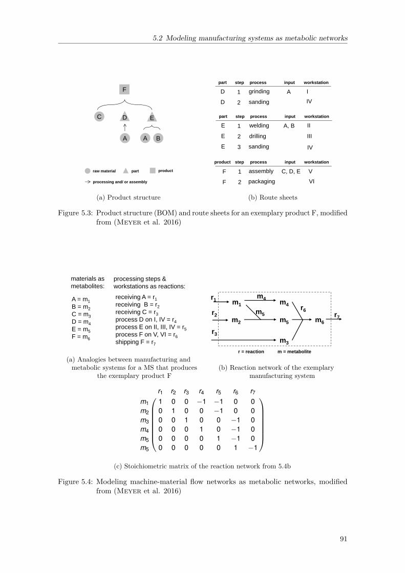
5.2 Modeling manufacturing systems as metabolic networks
F
A
A
material flow network
(for exemplary BOMs)
B
C
D E
F
G H part
1
1 1
2
2
product
4 5
1
3
5
0
0
D
raw material
E
A B
C
processing and/ or assembly
material – reaction network
R7
(a) Product structure
V
VI
A
material flow network
(for exemplary BOMs)
B
C
D E
F
G H
1
1 1
2
2
4 5
1
3
5
0
0
F
F
product workstation process step
assembly
packaging
1
2
input
C, D, E
I
IV
D
D
part workstation process step
grinding
sanding
1
2
input
A
II
III
E
E
E
part workstation process step
welding
drilling
sanding
1
2
3
input
A, B
IV
material – reaction network
R7 (b) Route sheets
Figure 5.3: Product structure (BOM) and route sheets for an exemplary product F, modifiedfrom (Meyer et al. 2016)
stoichiometric matrix for exemplary material – reaction network
reactions in
metabolic systems
are catalyzed by
enzymes, which are
seen as the
equivalent of
machines in the
analogy here
receiving A = r1
receiving B = r2
receiving C = r3
process D on I, IV = r4
process E on II, III, IV = r5
process F on V, VI = r6
shipping F = r7
processing steps &
workstations as reactions:
materials as
metabolites:
A = m1
B = m2
C = m3
D = m4
E = m5
F = m6
(a) Analogies between manufacturing andmetabolic systems for a MS that produces
the exemplary product F
stoichiometric matrix for exemplary material – reaction network
reactions in
metabolic systems
are catalyzed by
enzymes, which are
seen as the
equivalent of
machines in the
analogy here
m5
m4
m4
m6
m5
r6
r1 m1
m2
m3
r2
r3
r7
r = reaction m = metabolite
(b) Reaction network of the exemplarymanufacturing system
r1 r2 r3 r4 r5 r6 r7
m1 1 0 0 −1 −1 0 0m2 0 1 0 0 −1 0 0m3 0 0 1 0 0 −1 0m4 0 0 0 1 0 −1 0m5 0 0 0 0 1 −1 0m5 0 0 0 0 0 1 −1
(c) Stoichiometric matrix of the reaction network from 5.4b
Figure 5.4: Modeling machine-material flow networks as metabolic networks, modifiedfrom (Meyer et al. 2016)
91

5 Analyzing elementary flux modes in the resources-material flow network in MSs
5.3 Application of elementary flux mode analysis to a case studymanufacturing system9
5.3.1 Description of the analyzed system
In this section, EFMs will be calculated for the MS of a company that produces gearboxesand their accessories in a job shop MS. The resources in this MS are 51 machines usedfor different metal forming and machining processes. Although three of the 51 machinesare actually workstations for quality control and three are assembly stations, they will inthe following also be referred to as machines. The analyzed data set is one year worth offeedback data which was extracted from the company’s central production control software.The central production control software monitors the flows of material through the MS,recording for each operation on each machine the planned and actual start and end timesas well as the set-up times and work content. Every operation on a machine is uniquelyidentifiable and can be traced back to the final product it belongs to through the product’sBOM and route sheet, which were also extracted from the software.
In figure 5.5a, the material flows that took place between all machines in an exemplarytime span (week 10 of the analyzed year) are depicted as a network, with machines asnodes and material flows between the machines as links. Figure 5.5b gives an overview onsome of the characteristics and manufacturing performance values of the MS under study.
1
5
8
9
11
12
16
19
21
22
2324
26
29
33
35
36
43
44
45
46
34
25 39
17
3
27
14
47
15 7
49
32
4
6
10
18 30
38
41
40 13
20
2 42 48 37
31
28
(a) Exemplary network of machines (nodes) andmaterial flows (links) in week 10
characteristic valuenumber of different productsproduced in one year
544
average number of differentproducts per week
61
number of operations executedin one year
32.120
average planned operation time(in days)
3.12
average actual operation time(in days)
7.8
average lateness of an operation(in days)
24
(b) Characteristics and performance values ofthe analyzed manufacturing system
Figure 5.5: Analyzed real case data, modified from (Meyer et al. 2016)
Although the possibility of taking alternative routes exists for certain products (somemachines are able to perform the same manufacturing processes), the company in the casestudy only attributes one route sheet with one fixed route to each product.
9Parts of this section have been published in similar form in (Meyer et al. 2016).
92

5.3 Application of elementary flux mode analysis to a case study manufacturing system
5.3.2 Elementary flux mode calculation and discussion of results
Using 3131 BOMs and route sheets extracted from the companies production controlsoftware, a stoichiometric matrix for the real case data was created according to theanalogies introduced in section 5.2. Computation of the EFMs was done using the freelyavailable efmtool in MATLAB (Terzer and Stelling 2008). As a result of the largeamount of different products being manufactured per year (see figure 5.5b), the calculationof EFMs based on the manufacturing network that results from a year’s worth of feedbackdata is computationally challenging, with the stoichiometric matrix reaching a size ofabout 3000 columns x 3000 rows for one entire year. Moreover, the demand for producttypes and amounts significantly varies from week to week, so that an analysis on a yearlybasis would conceal these fluctuations. Additionally, planning and scheduling in the MSis carried out daily to weekly (which is also the time span range for planned and actualoperation times, see figure 5.5b), so that performance effects should be measured on thisbasis. The yearly data was therefore divided into weekly time bins. For each time bin, theproducts that were manufactured and the corresponding operations and material flowsbetween the machines were extracted. Then all the manufacturing operations necessary tomanufacture the products were derived from the feedback data and thus a weekly materialflow network for every time bin was created, following the analogy described in section 5.2.An exemplary material flow network for week ten is given in 5.5a. The number of EFMsper time bin t (et) was then calculated using the stoichiometric matrices of the weeklymaterial flow networks. Figure 5.6 gives an overview on the different amounts of EFMsper time bin.
0 5 10 15 20 25 30 35 40 45 500
10
20
30
40
50
60
70
80
num
ber
of E
FM
s (e
)
time bin (t)
Figure 5.6: Number of EFMs per time bin (et), modified from (Meyer et al. 2016)
As assumed, the value of et does not stay the same in every time bin, as the product mix isdifferent from time bin to time bin. In case no alternative work plans or materials and thusno alternative routes exist in the system, the number of EFMs in each time bin correspondsto the number of different products produced in that time bin. For each product there isexactly one possible way that leads from one or more raw materials to the final product.
93

5 Analyzing elementary flux modes in the resources-material flow network in MSs
As an example, 39 different products are being produced in time bin one, while in time bineleven, 79 different products are being produced (see figure 5.6). Comparing this findingto biological systems, the number of EFMs to be found for example in the metabolism ofbacteria is a lot higher for most biomass components produced (Stelling et al. 2002).This is primarily caused by the fact that in metabolic systems, many of the occurringreactions are reversible, that the same final product can be produced via different paths,and that final products can be produced from different types of substrates which throughdifferent reactions yield the same product in the end. The case that a product in a MScan either be manufactured from one type of raw material (e.g. steel) or from a differenttype of raw material (e.g. plastic) does not occur in our analyzed dataset, and is hardlyoccurring in any industrial production system. Therefore the number of EFMs found inMSs is generally lower than in biological systems.
5.3.3 Machine knock-out study and discussion of results
In metabolic systems, the disturbance of a gene deletion can occur due to a multitude ofreasons and can have different effects on the production of biomass of the metabolic system.Following the methodology of Stelling et al. (2002) and the analogies drawn betweenmetabolic and MSs, the effects a removal of a machine (e.g. a machine breakdown) has onthe MS and whether EFMs can serve as a predictor for this are analyzed in the following.To pretend that a machine is not available in a time bin, all reactions that a machine ispart of are removed from the stoichiometric matrix, then the number of EFMs that are leftin time bin t when machine i is unavailable (et (i)) is calculated. The average number ofEFMs that are removed if machine i is under breakdown in time bin t (∆et (i)) is calculatedas
∆et (i) = et − et (i) (5.1)
Based on this, the average percentage of EFMs that are left under knock-out of a machinei over all time bins t (pe(i)) can be calculated as
pe(i) =⟨∆et (i)
et
⟩t
(5.2)
where the brackets denote the average over all time bins t . Figure 5.7 shows pe(i); errorbars in this figure arise from the standard deviation corresponding to the average over alltime bins t (see equation 5.2).
The number of EFMs that is deleted when a machine is not available indicates how manydifferent products cannot be produced any more. As the sheer number of products alonedoes not allow conclusions as to the importance of the product and thus the severity of itsunavailability, the average amounts of products that are affected by the breakdown of amachine were also analyzed. The product amounts are affected by machine unavailabilityin a similar way as the product numbers: both values correlate with an average Pearson’slinear correlation coefficient of 0.93 and a standard deviation of 0.08, with a significance
94

5.3 Application of elementary flux mode analysis to a case study manufacturing system
0 5 10 15 20 25 30 35 40 45 500
0.2
0.4
0.6
0.8
1
machine (i)
aver
age
perc
enta
ge o
f EF
MS
del
eted
(p e)
Figure 5.7: Average percentage of EFMs that are deleted if a machine is not available(pe(i)); error bars denote the standard deviation from the average, modifiedfrom (Meyer et al. 2016)
on the 0.1 percent level. Thus the conclusion is drawn that the number of EFMs can serveas an indicator of a machine’s significance. However, as the company only attributes oneroute per product (also more would be technically possible) the full potential of EFManalysis has not been completely demonstrated yet: if products were produced via differentraw materials, if reactions were reversible, or if alternative production paths (route sheets)existed, this would result in a differently structured stoichiometric matrix. In case of aresource breakdown, the number of EFMs would not change as drastically as it is changingnow, since many more alternative production paths would be possible.
5.3.4 Correlation of elementary flux modes and manufacturing performanceindicators
In addition to the previously shown relation of EFMs to number and amounts of productsmanufactured, it should further be demonstrated that the structural measure of EFMs doesdisplay a significant relation to dynamic MSP indicators and can thus serve as an indicatorof machine significance. Therefore it is analyzed if machines whose deletion results in adeletion of a high number of EFMs are correlated to traditional indicators of MSP. As MSPindicators, lateness and work content were chosen. Lateness is calculated as the averagelateness of all operations mt that are carried out on a machine i in time bin t (lt (i))
lt (i) = 〈|am(i)− pm(i)|〉mt(5.3)
where am(i) is the actual end date of operation m on machine i, and pm(i) is the plannedend date of operation m on machine i . The brackets denote the average over all operations
95

5 Analyzing elementary flux modes in the resources-material flow network in MSs
mt that take place in time bin t . The average work content of operations per machine pertime bin (wt (i)) is calculated as
wt (i) = 〈om(i)〉mt(5.4)
where om(i) is the work content of operation m on machine i (measured in hours) and mt isthe number of operations on machine i in time bin t . The brackets denote the average overall operations mt that take place in time bin t .
Furthermore, the correlation of MSP indicators and EFMs is compared to the correlationbetween MSP indicators and two indicators that are frequently used as measures incomplex network science as well as between MSP indicators and a classical indicatorof machine significance from the manufacturing domain. As indicators from complexnetwork science, nodedegree (nd) and betweenness centrality of a node (bc) (as introducedin section 2.3.2) of the machine-material flow graph are used. In the machine-material flowgraph, a node corresponds to a machine, while the links between the nodes correspond tothe material flows between the machines. The nd of a node i in time bin t (ndt (i)) is thesum of all incoming and outgoing links of a node in the network of time bin t . The bc of anode i in time bin t (bct (i)) is calculated as suggested by Freeman (1977)
bct (i) =∑
jk
σt (j , i , k )σt (j , k )
(5.5)
where i is the number of the node, σt (j , i , k ) is the number of shortest paths between node jand k that pass through node i in time bin t , and σt (j , k ) is the total number of shortestpaths from node j to k in time bin t . As a classical indicator for machine significance,static manufacturing complexity (mc) as suggested by Calinescu et al. (1998) was chosen.The mc of a machine i in time bin t (mct (i)) is calculated as
mct (i) = −Ns∑s=1
ps,t (i)log2ps,t (i) (5.6)
where s is the state of a machine (either idle, working, or set up), Ns is the number ofdifferent states s, and ps,t is the probability of machine i being in state s in time bin t .Static complexity in MSs serves as a measure of the difficulty to produce the requirednumber and type of products in the required period of time (Calinescu et al. 1998).
To show the relation between the indicators for machine significance (∆et (i), ndt (i), bct(i),mct (i)) and the performance of the machines (lt (i), wt (i)), Pearson’s linear correlationcoefficient (cp) between each machine significance indicator and the two performancemeasures for all machines per time bin (see figure 5.8 and figure 5.9) was calculated. Theerror bars in the figures represent the mean value and standard deviation of the correlationsthat resulted from 100 random shuffles of the values of the machine significance indicatorand the performance measures for the respective time bin.
96

5.3 Application of elementary flux mode analysis to a case study manufacturing system
0 5 10 15 20 25 30 35 40 45 50−0.5
0
0.5
1co
rrel
atio
n (c
p)
∆ e & lrandom permutation ∆ e & l
0 5 10 15 20 25 30 35 40 45 50−0.5
0
0.5
1
corr
elat
ion
(cp)
nd & lrandom permutation nd & l
0 5 10 15 20 25 30 35 40 45 50−0.5
0
0.5
1
corr
elat
ion
(cp)
bc & lrandom permutation bc & l
0 5 10 15 20 25 30 35 40 45 50−0.5
0
0.5
1
corr
elat
ion
(cp)
time bin (t)
mc & lrandom permutation mc & l
Figure 5.8: Correlations of the different indicators (∆e, nd , bc, mc) with average machinelateness (l) per time bin (t). The error bars denote the average correlation andstandard deviation of 100 random permutations of the different indicators andthe average machine lateness, modified from (Meyer et al. 2016)
While the structural indicators nodedegree per machine (ndt (i)) and betweenness centralityper machine (bct (i)) only exhibit few to no correlation values with work content (wt (i)) thatare higher than the correlations of the randomly shuffled ndt (i) and bct (i) values, there areclear, non-random correlations between the deleted elementary modes per machine (∆et (i))and the work content of a machine (wt (i))(see figure 5.9). Similarly, the correlation valuesbetween wt (i) and mct (i) are for most of the time bins higher than the correlations betweenwt (i) and a random shuffle of mct (i), yet this does not seem so surprising as the calculationof mct (i) is based on work content and set-up times (see equation 5.6), and set-up times inthe company under study are extremely low.
Even more strikingly, ∆et (i) also shows several correlation values with machine lateness (lt (i))that are higher than the correlations of the randomly shuffled ∆et (i) values and machine
97

5 Analyzing elementary flux modes in the resources-material flow network in MSs
0 5 10 15 20 25 30 35 40 45 50
−0.5
0
0.5
1co
rrel
atio
n (c
p)
∆ e & wrandom permutation ∆ e & w
0 5 10 15 20 25 30 35 40 45 50
−0.5
0
0.5
1
corr
elat
ion
(cp)
nd & wrandom permutation nd & w
0 5 10 15 20 25 30 35 40 45 50
−0.5
0
0.5
1
corr
elat
ion
(cp)
bc & wrandom permutation bc & w
0 5 10 15 20 25 30 35 40 45 50
−0.5
0
0.5
1
time bin (t)
corr
elat
ion
(cp)
mc & wrandom permutation mc & w
Figure 5.9: Correlations of the different indicators (∆e, nd , bc, mc) with average machinework content (w) per time bin (t). The error bars denote the average correlationand standard deviation of 100 random permutations of the different indicatorsand the average machine work content, modified from (Meyer et al. 2016)
lateness (lt (i)) (see Figure 5.8). None of the other structural based indicators (ndt (i), bct (i))exhibit this feature. Note that the correlations between both performance values and ∆et (i)are predominantly negative, while all other correlations are mostly positive. This meansthat with a higher number of EFMs that is deleted by the breakdown of a machine, thelateness of this machine becomes lower. For the real world scenario, this means the higherthe significance of a machine for the MS, the lower its lateness.
To assess the overall suitability of the indicators for machine importance, a distance measure(d(h, v )) that only considers the correlation coefficients (c) of those time bins where thecorrelation coefficient of the significance indicators (h) and the performance values (v) areoutside the random field defined by the 100 random shuffles of the significance indicators,is calculated. The distance measure (d) is calculated as
98

5.3 Application of elementary flux mode analysis to a case study manufacturing system
d(h, v ) = 〈cu(h, v )−maxu(h, v )〉u (5.7)
where the brackets denote a sum over all time bins u, which is the number of time binsin which the correlation coefficient of bin u (ru) is higher (for negative correlations lower)than the standard deviation of the average correlation coefficient of the randomly shuffledsignificance indicator and the performance indicator of time bin u (maxu). Figure 5.10shows the distance measure for the correlations between lateness (lt (i)) and work content(wt (i)) with the machine significance indicators δet (i), ndt (i), bct (i), and mct (i) from figure 5.8and 5.9.
(a) Distance measure for indicators and lateness(l)
(b) Distance measure for indicators and workcontent (w)
Figure 5.10: Distance measure (d) of the different indicators ∆e, nd , bc, mc, modifiedfrom (Meyer et al. 2016)
The highest absolute distance measure is denoted for the correlation between machinelateness (lt (i)) and the number of elementary flux modes deleted by a machine breakdown(∆et (i)) (see figure 5.10a). The distance measure exhibits positive values for the correlationsbetween ndt (i), bct (i), mct (i), and (lt (i)) since the majority of the significant correlationsbetween them are positive (see figure 5.8). As the majority of significant correlationsbetween the number of deleted EFMs (∆et (i)) and lateness (lt (i)) are negative, the distancemeasure is also negative, but still exhibits the biggest absolute value and can thus beseen as the most suitable predictor for machine lateness. For work content, ∆et (i) showsthe second best value of d(h) and thus suitability, after manufacturing complexity. Theindicators based on structural aspects of the underlying machine-material flow graph (ndt (i),bct (i)) do not exhibit any significant correlations with machine performance indicators.
99

5 Analyzing elementary flux modes in the resources-material flow network in MSs
5.4 Application of elementary flux mode analysis to the test MSconfigurations
5.4.1 Elementary flux mode calculation and discussion of results
To demonstrate the applicability of EFM calculation in a larger scale of MSs, the EFMsof each of the 81 MS configurations created in section 3.4 are calculated in the following.Similar to the EFM calculation in the case study (section 5.3), the EFMs are calculatedusing the Matlab software efmtool (Terzer and Stelling 2008). Corresponding to theobservations in the case study data set, EFMs cannot be calculated for all of the 81 MSconfigurations, due to the large size of some of the stoichiometric matrices. This is also acommon issue in metabolic systems (see also explanations in section 5.1), and one of themajor drawbacks of EFM analysis. The number of EFMs e per MS configuration g (eg)are depicted for 54 of the 81 MS configurations in figure 5.11. A complete list of eg valuescan be found in Appendix E.
0 5 10 15 20 25 30 35 40 45 50 5510
0
101
102
103
104
105
106
107
MS configuration (g)
num
ber
of E
FM
s (e
)
Figure 5.11: Number of EFMs per MS configuration (eg) for 54 of the 81 MS configurations
Compared to the case study data analyzed in section 5.3, the average number of EFMs perMS configurations is notably higher in the generated MS configurations, with an averageof 386283 EFMs per configuration. However, this value is also subject to a very largestandard deviation of 321645, as the number of EFMs ranges between a minimum of 10 anda maximum of 2239928. The reason for this is that within the generated MS configurations- as opposed to the real case study - alternative machines and thus alternative paths forparts and products exist.
100

5.4 Application of elementary flux mode analysis to the test MS configurations
5.4.2 Machine knockout study and discussion of results
Similar to the approach for the case study data and the approach by Stelling et al.(2002) in metabolic systems, the impact of machine knockouts on the number of EFMs isanalyzed in the following. Compared to the case study data in the previous section, theEFMs are now calculated per MS and not per time bin. This is due to the fact that theMS configurations were artificially created, hence no real data to split into bins exists. Topretend that a machine is not available in a configuration, all reactions that a machine i ispart of are removed from the stoichiometric matrix of the configuration g and the residingnumber of EFMs that are left (eg(i)) is calculated. The average number of EFMs e thatare removed under breakdown in a configuration g (∆eg) is then calculated as
∆eg = 〈eg − eg(i)〉g (5.8)
where the brackets denote the average over all configurations g. Based on this, the averagepercentage of EFMs that are left under knock-out of the machines pe per configuration g(pe(g)) can be calculated as
pe(g) =⟨∆eg
eg
⟩g
(5.9)
where the brackets denote the average over all configurations g. Figure 5.12 shows pe(g);error bars in this figure arise from the standard deviation corresponding to the averageover all machines i (see equations 5.8 and 5.9). A complete list of pe(g) values per MSconfiguration can be found in Appendix E.
0 5 10 15 20 25 30 35 40 45 50 550
0.2
0.4
0.6
0.8
1
MS configuration (g)
aver
age
perc
enta
ge o
f EF
Ms
dele
ted
(pe)
Figure 5.12: Average percentage of EFMs that are deleted per configuration with a machineknockout (pe(g)); error bars denote the standard deviation from the average
101

5 Analyzing elementary flux modes in the resources-material flow network in MSs
Compared to the EFM analysis on the case study data, the average percentage of EFMsthat are deleted by machine knockouts per configuration is strikingly higher (73%) thanthe average percentage of EFMs that are deleted by machine knockouts per bin in thereal case data set (35%). However, while a deletion of an EFM in the real case data isequal to the "loss" of a product, the deletion of an EFM in the MS configurations does notautomatically signify a product loss, as alternative routes for product manufacture exist.As it cannot be concluded from this number alone whether a MS can be classified as moreor less robust against machine breakdowns, the number of EFMs per MS configuration(eg) and the average percentage of EFMs that are deleted by machine knockout (pe(g)) arecorrelated to the robustness (r) of the MS configurations in the following section.
5.4.3 Correlation of robustness and elementary flux modes
In order to analyze the relation between robustness of a MS and EFMs, the calculated EFMvalues eg and pe(g) are correlated to MSP robustness r (as defined in 3.1). Figure 5.13shows the relation between robustness (r) and the EFM values eg and pe(g) of the 54 MSconfigurations.
The linear correlation between r and eg is positive, with a Pearson’s correlation coefficient ofcP = 0.27 and a p-value of 0.07, indicating no strongly significant correlation, yet comparedto the correlations of some of the complex networks measures and nestedness indicatorsbeing one of the more significant correlations found within the analysis presented in thisthesis. The linear correlation between r and pe(g) is also positive, exhibiting the yet highestlinear correlation coefficient of all analysis - cP = 0.39 - with a strong significance of p =0.007. The rank correlation between r and eg is also positive, showing the highest rankcorrelation coefficient of all conducted analysis which lies at cS = 0.51, with an extremelysignificant p-value of 0.00. The rank correlation between r and pe(g) is as well positive, witha correlation coefficient of cS = 0.39 and highly significant p-value of 0.007. From theseresults it is concluded that the higher the eg or pe(g) values of a MS configuration are, thehigher is their robustness of the MSP measure lateness against machine breakdowns in therespective MS configuration. The high significance levels (compared to the results for theprevious indicators) renders both values the most suitable indicators for MS robustness.
102
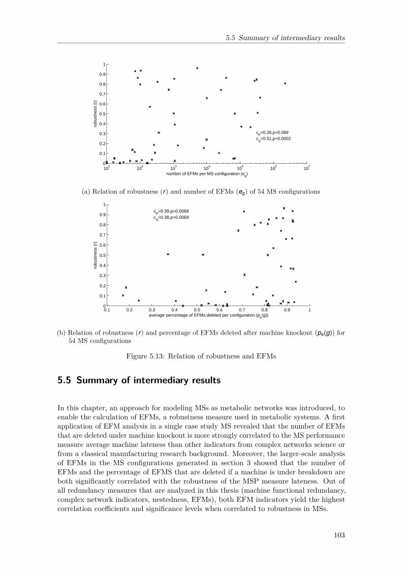
5.5 Summary of intermediary results
101
102
103
104
105
106
107
0
0.1
0.2
0.3
0.4
0.5
0.6
0.7
0.8
0.9
1
robu
stne
ss (
r)
number of EFMs per MS configuration (eg)
cP=0.26,p=0.069
cS=0.51,p=0.0002
(a) Relation of robustness (r) and number of EFMs (eg) of 54 MS configurations
0.1 0.2 0.3 0.4 0.5 0.6 0.7 0.8 0.9 10
0.1
0.2
0.3
0.4
0.5
0.6
0.7
0.8
0.9
1
robu
stne
ss (
r)
average percentage of EFMs deleted per configuration (pe(g))
cP=0.39,p=0.0068
cS=0.38,p=0.0069
(b) Relation of robustness (r) and percentage of EFMs deleted after machine knockout (pe(g)) for54 MS configurations
Figure 5.13: Relation of robustness and EFMs
5.5 Summary of intermediary results
In this chapter, an approach for modeling MSs as metabolic networks was introduced, toenable the calculation of EFMs, a robustness measure used in metabolic systems. A firstapplication of EFM analysis in a single case study MS revealed that the number of EFMsthat are deleted under machine knockout is more strongly correlated to the MS performancemeasure average machine lateness than other indicators from complex networks science orfrom a classical manufacturing research background. Moreover, the larger-scale analysisof EFMs in the MS configurations generated in section 3 showed that the number ofEFMs and the percentage of EFMS that are deleted if a machine is under breakdown areboth significantly correlated with the robustness of the MSP measure lateness. Out ofall redundancy measures that are analyzed in this thesis (machine functional redundancy,complex network indicators, nestedness, EFMs), both EFM indicators yield the highestcorrelation coefficients and significance levels when correlated to robustness in MSs.
103

5 Analyzing elementary flux modes in the resources-material flow network in MSs
For structural indices of complexity measurement, it has been argued that they show po-tential to be utilized to evaluate MS designs in the design or re-design phase of MSs (Kuz-gunkaya and ElMaraghy 2006; Chryssolouris et al. 2013). Likewise, as EFMsare significantly correlated to robustness, it is concluded that they denote a topologicalmeasure that gives an indication of how important a resource is for MSP robustness againstmachine breakdowns. Similar to the suggestions in Li et al. (2009) or Li (2009), wherebottlenecks are detected using a data-driven method, EFMs could serve as a measureto detect resources that are crucial for the performance and functioning of the MS. Asalso argued in Zhao and Wallace (2016), redundant resources could then be added forthose resources that were identified as crucial resources by EFM analysis. In the followingchapter, it is thus elaborated on how structural indicators such as the suggested machinefunctional redundancy (see chapter 3) or EFMs can be integrated in methods for MSD tocreate RMSD methods.
104

6 Designing robust manufacturing systemswith redundancy considerations
In the previous three chapters, it was analyzed how different structural indicators measuringredundancy in MSs are related to robustness. It was shown that some of the redundancyindicators are significantly correlated to robustness in MSs and can thus be regarded assuitable predictors for the robustness of lateness to machine breakdowns in MS. As statedin the motivation section, this thesis focuses on how the long term adequate amount ofresources in job shop MSs can be designed to achieve a high MS robustness. It is thuspresented in this chapter how the previously analyzed structural redundancy indicators canbe used for RMSD. Existing methods for designing MSs, and in particular determining theadequate amount of resources in job shop MSs, have been presented in section 2.1.3, whileapproaches for RMSD have been introduced in section 2.2.3. In the first section 6.1 of thischapter, possibilities for integrating structural redundancy indicators into the presentedmethods for resource determination in job shop MSs are pointed out. Furthermore, as therequirements for initial MSD differ from the re-design of a MS, a concept for assessingrobustness of an existing MS in case of re-design is suggested. It was also emphasizedin section 2.1.3 that the consideration of trade-offs plays an important role in MSD. Asintroduced in section 1, a potential trade-off exists between robustness - if it is caused byredundancy - and efficiency. Resources cannot just be added infinitely to a MS, as each ofthem incurs costs. Section 6.2 gives a more detailed description of this potential trade-off,both in biological systems and MSs, and conceptually describes how it can be consideredin MSD. The last section 6.3 of this chapter discusses the advantages and disadvantagesof the use of structural indicators for MSD, with a focus on the redundancy indicatorsanalyzed within this thesis.
6.1 Potential use of structural redundancy measures inmanufacturing system design procedures 10
As introduced in section 2.1.3, the main methods for determining the adequate amount ofresources when designing job shop MSs are simple analytical, mathematical optimization,queuing, and simulation models. In the presented simple analytical models, a structuralindicator such as number of EFMs in the MS configuration or nestedness of the parts-resource network cannot be integrated directly as a part of the model. These approachesare based on the simplified assumptions that the number of resources can be determinedby multiplying operation time per product and number of products needed (compare alsotable 2.1). Similarly, structural indicators such as EFMs cannot be directly integrated intoqueuing models of MSs, as these consist of the characteristics mentioned in section 2.1.3.10Parts of this section have been published in similar form in (Becker and Meyer 2014).
105

6 Designing robust manufacturing systems with redundancy considerations
If such design approaches are chosen, structural indicators can be used to evaluate theconfigurations created with the approaches, e.g. a high number of EFMs per configurationindicating high robustness and a low number of EFMs indicating low robustness towardsmachine breakdowns. This approach is conceptually depicted in figure 6.1, where variablesused to create alternative MS configurations with analytical, queuing, or simulations modelsare suggested. The created alternative configurations are then evaluted regarding theamount of EFMs they feature. The MS with the highest amount of EFMs can then bechosen as the most robust system.
III.
create different alternative MS
configurations
I.
II.
alternative MS
configurations
calculate structural indicators,
e.g. EFMs, to evaluate
alternative MS configurations
simple analytical, queuing, or
simulation model
model set-Up MS configurations
evaluation
EFMs configuration I: 3
EFMs configuration II: 5
EFMs configuration III: 7
input variables
number of products to be
produced
manufacturing processes
per product
processing times per
manufacturing process
output variables
number of machines
Figure 6.1: Evaluation of a MS configuration’s robustness
Mathematical optimization models however offer the possibility of incorporating structuralindicators into the models themselves. In the introduced mathematical optimizationapproaches for resource dimensioning in job shop MSs (see section 2.1.3), mostly costfunctions are used as targets for the mathematical optimization models, which means thatthe models determine the amount of resources in a way that the overall costs for the MSconfiguration (e.g. investment costs) are lowest. This usually creates MS configurationswith just as many resources as needed to fulfill a given demand, and no excess resourcesas this would not deliver the most cost-efficient MS configuration solution according tothe target function of the optimization model. Integrating structural indicators into thetarget functions of optimization models would directly allow optimizing a configuration forthe desired structural measure, i.e. creating configurations with high or low levels of therespective structural indicator. Figure 6.2 gives an exemplary presentation of which inputsand target function variables are required for such a procedure.
The approach described in figure 6.2 is similar to the existing procedures for RMSD, ofwhich all reviewed ones used mathematical optimization models (see section 2.2.3). Two ofthe introduced RMSD approaches used structural measures to asses the robustness of a MSand integrated them into an optimization model to create a robust MS (Scholz-Reiteret al. 2011; Sharda and Banerjee 2013). However, in these approaches it was notshown that the utilized structural indicators are actually linked to the robustness of theperformance of the MSs, which is the case for EFMs and MS performance measuredby lateness. Moreover, none of the existing approaches for RMSD considered the MSperformance indicator lateness as a robustness criterion.
106

6.1 Potential use of structural redundancy measures in MSD procedures
create one MS configuration
with an optimized amount of
the structural indicator, e.g.
EFMs
MS configuration
mathematical optimization model that
contains structural indicator in target
function, e.g. EFMS
model set-up
exemplary input variables
number of products to be produced
manufacturing processes per
product
processing times per manufacturing
process
exemplary target function
structural indicators
exemplary output variables
optimal number of machines
Figure 6.2: Creation of a robust MS configuration
The above described potential usage of structural indicators for the design of MS differsfrom re-design of MSs. The previous considerations for the use of structural indicatorsfor MS design are based on a robustness measure that requires the comparison of MSperformance in perturbed and unperturbed conditions of a MS. This is easily applicableif a model of a MS exists, like in section 3.4.3, where robustness was measured as theratio of the performance measures lateness in perturbed and unperturbed scenarios. Butif robustness should be measured in existing MSs of which no model exists to simulateperturbed and unperturbed conditions, the approach for measuring robustness has to bechanged. Figure 6.3 gives a conceptual description of how robustness of existing MSs canbe assessed. Similar to the definition of robustness in a modeling state (see section 3.1), forassessing robustness of an existing MS the system under study is the MS of a manufacturingorganization. The property or function that should be robust in the face of perturbationsis MSP, which varies over time (t) (see figure 6.3). Yet the fact that MSP varies slightlyover time does not necessarily imply that the MS is not robust. A slight change in MSPshould not directly lead to the system being classified as not robust, it should ratherbe possible for the performance to slightly fluctuate in a defined invariance or tolerancecorridor around a mean value tp. However, if the MSP is constantly below a target value,the system cannot be described to be robust. Therefore the invariance measure should alsoinclude a time-related component, which is the time span for which the performance isallowed to deviate below the average value, depicted as tt in figure 6.3. The behavior ofthe MSP with regard to the set invariance measures (tt , tp) determines whether a MS isregarded as robust or not. In figure 6.3, the first perturbation (p1) causes a decrease of theMSP, which is still within tp, and MSP reaches the average again within tt . Yet for thesecond perturbation (p2), MSP is decreased below the average for longer then tt . If p1 andp2 belong to the set of defined perturbations, the system in the conceptual depiction doesnot classify as a robust system.
This assessment method has to be tailored to a MS and its conditions, thus it is not possibleto compare existing systems with regard to their robustness with this approach.
107

6 Designing robust manufacturing systems with redundancy considerations
MSP
t
tp
tt
p2
tt
p1
Figure 6.3: Assessing the robustness of an existing MS, modified from (Becker andMeyer2014)
6.2 Considering the trade-off between redundancy-inducedrobustness and cost-efficiency
As introduced in section 2.1.2, a trade-off can exist between the targets of efficiency androbustness in MSs. Such a conflict between robustness and efficiency is also well-known anddescribed in a biological context. In Goerner et al. (2009), a trade-off between sustain-ability (which is in their definition closely related to the robustness definition used in thisthesis) and efficiency in ecosystems is described. As depicted in figure 6.4, Ulanowiczet al. (2009) and Goerner et al. (2009) hypothesize that sustainability in ecosystems, i.e.the survival of species, is in a trade-off relationship with efficiency, where too low diversityin number of species (high efficiency) causes brittleness of the ecosystem, while too highdiversity (low efficiency) causes stagnation within the ecosystem. They analyze severaldata sets of real ecosystems and find that all systems are positioned in an optimal balancebetween too high and too little efficiency, which they refer to as a window of vitality.
su
sta
ina
bili
ty
diversity
(too high efficiency) (too little efficiency)
brittleness stagnation optimal balance
window of vitality
= real data from ecosystems
Figure 6.4: Trade-off between efficiency and resilience in ecologic systems, modifiedfrom (Goerner et al. 2009)
Stelling et al. (2002) in their work also conclude that in metabolic networks, a trade-offis found between flexibility - related to robustness - and efficiency. Similarly, Morine et al.(2009) argue that the more efficient metabolic networks are, the less robust they tend tobe, which they show in an analysis of 105 real metabolic networks. Apart from biologicalsystems, the trade-off between efficiency and robustness is also known in man-made systems
108

6.2 Considering the trade-off between redundancy-induced robustness and cost-efficiency
such as supply chains (Shukla et al. 2011; Ivanov et al. 2014). Shukla et al. (2011) forinstance describe, analyze, and optimize the trade-off between robustness of supply chains,caused by built-in risk tolerance, and efficiency of supply chains, represented by operating,transport, and handling costs.
In a manufacturing context, a trade-off that is similar to the ones described above inbiological systems was also found and investigated for the capacity planning of MSs, whichis a short-term phase of MSD (see section 2.1.3). As capacity requirements can be dynamic(i.e. they change over time when customer demand changes), different planning strategiescan be chosen in order to determine the adequate amount of capacity for a MS (Kobylka2000): capacity can be installed in excess over the peaks of demand, as an average, or exactlycorresponding to the demand (see figure 6.5). It was shown by Kobylka (2000) that eachof these strategies has a different relation to other performance measures and is suitablefor different production environments. Especially the excess capacity strategy stands ina trade-off with investments which can be seen in figure 6.5). This denotes a trade-offbetween robustness (induced by high excess capacity) and efficiency (low investments).
ca
pa
city
ca
pa
city
ca
pa
city
time
time
time
installation of
capacity in
excess of
demand
installation of
capacity
corresponding
to demand
installation of
“average”
capacity and
smoothing of
demand
installed
capacity
installed
capacity
installed
capacity
required
capacity
required
capacity
required
capacity Investm
ents
Thro
ughput tim
e
Pla
nnin
g a
nd c
ontr
ol effort
Fle
xib
ility
Figure 6.5: Trade-offs in capacity dimensioning, modified from Kobylka (2000)
The described trade-offs between robustness and efficiency in biology, supply chain, andmanufacturing contexts are conceptually similar to the trade-off that arises when designingrobust MSP by increasing resource redundancy, which is the underlying assumption of thisthesis explained in section 3.3 and conceptually illustrated in figure 3.3. It is describedthere that the increase of machine redundancy and machine functional redundancy alsoincreases the robustness of the MSP lateness against machine breakdowns. However, theprovision of such redundancy requires higher costs, for example for machines with theability to conduct several manufacturing processes (machine functional redundancy). Thisredundancy renders the MS more robust, however the cost-efficiency of such MSs withredundancies is lower than the one of systems without redundancy. Similar to the relationbetween robustness and redundancy, this trade-off between robustness and efficiency canalso be conceptually depicted. In figure 6.6, the assumption that efficiency in MSs decreaseswith increasing robustness and redundancy is graphically depicted. As it was shown in theprevious sections of this thesis that robustness increases with redundancy, both values areshown on the y-axis of figure 6.6. Contrary to the complementary relationship between
109

6 Designing robust manufacturing systems with redundancy considerations
robustness and redundancy (one increases with the increase of the other), efficiency isassumed to be in a conflicting relationship with both values (one decreases with the increaseof the other). However, it is not known how this relationship behaves exactly, hence twodifferent potential curves in figure 6.6 indicate different possible relations.
efficiency
redundancy/
robustn
ess
Figure 6.6: Trade-off between robustness/redundancy and efficiency, modified from (Meyeret al. 2013)
Thus when striving for a robust design of a MS, it should not only be investigated howrobustness is influenced by redundancy, but also how increased redundancy affects cost-efficiency of the MS under study. A possibility to consider this trade-off in MSD is theutilization of trade-off curves, which were introduced in section 2.1.3 as an important meansof MSD. During the design process, MS configurations with different robustness values canbe evaluated with regard to their efficiency, leading to the creation of a trade-off curve, asconceptually depicted in figure 6.7. Here it is shown how for two different MSs, alternativeconfigurations with different amounts of redundancy are created. These alternatives canthen be evaluated regarding their cost-efficiency, for example by recording their investmentor handling costs. This results in two different curves of which each has a unique fitdetermined by the behavior of the respective MS.
cost-efficiency
redundancy/ ro
bu
stn
ess
system configuration alternatives evaluation
I
II
III
I
II
III
manufacturing system 2
I. few redundancies
II. medium redundancies
III. many redundancies
manufacturing system 1
machine configurations MS 1 configurations MS 2 material flow
I. few redundancies
II. medium redundancies
III. many redundancies
Figure 6.7: Considering the trade-off between efficiency and robustness in RMSD, modifiedfrom (Meyer et al. 2013)
110

6.3 Discussion of the use of structural redundancy indicators for RMSD
6.3 Discussion of the use of structural redundancy indicators forrobust manufacturing system design
The previous section has given an insight on how structural redundancy indicators canbe used for RMSD. In this preceding section, it is discussed which advantages anddisadvantages the use of structural redundancy indicators bears for RMSD. The discussionconsiders technical calculation aspects as well as aspects concerning the suitability of thetransfer of concepts from a biological context to a manufacturing context. There are severalbenefits and drawbacks that are shared by all structural redundancy indicators analyzed inthis thesis. These will be presented first, followed by a detailed analysis per indicator.
All structural redundancy indicators analyzed in this thesis are calculated based on staticinformation about a MS configuration, such as the number of machines or processes permachine, the BOMs or route sheets. This kind of information is easily accessible within amanufacturing organization from existing databases or software like production planningprograms. If a significant correlation between a structural redundancy indicator androbustness exists, it is possible to draw a conclusion about the amount of robustness of aMS configuration from only calculating the level of the structural redundancy indicator.Other standard methods used for determining the amount of robustness, like queuing,optimization, or simulation models (see section 2.1.3), would be more time- and effort-intensive to build and apply. The benefits of such static, structural indicators have alsobeen analyzed and described for assembly systems in a manufacturing contexts by Samyand ElMaraghy (2012). They use a regression analysis and reveal a relationship betweenpart complexity and assembly equipment complexity. Their model shows that the assemblyequipment complexity increases as part complexity increases in a nonlinear relation, meaningthat in an early design state when only the parts are known, conclusions can already bedrawn as to how complex the corresponding assembly system has to be (Samy andElMaraghy 2012).
However, structural indicators in general are also reflected critically by many authors. FoxKeller (2005) critically discusses the growth and popularity of complex network measures,and in particular the tendency of transferring findings on networks among different disci-plines. Similarly, Stumpf and Porter (2012) argue that many of the findings concerningpower laws in complex network research are not backed up enough from a statistical pointof view. In Lima-Mendez and Helden (2009) it is claimed that many of the complexnetworks findings in biological networks, such as degree distributions following power lawsor metabolic networks being scale-free networks, are not universally true and are sometimesresults of sampling artefacts or improper data representation. In Alderson (2008), it isfurther challenged if the application of complex network measures in operations researchor engineering domains is beneficial.
Machine and machine functional redundancy
The two indicators machine and machine functional redundancy are both calculatedbased on static information about a MS configuration, which are the number of machinesor the number of processes per machine. As they utilize similar input data as for examplemeasures for flexibility in MSs they are closest to measures from a classical manufacturing
111

6 Designing robust manufacturing systems with redundancy considerations
background. However, a significant correlation to robustness was only revealed for machinefunctional redundancy (see chapter 3), which makes this measure a more suitable predictorfor the amount of robustness of a MS configuration than machine redundancy.
Nestedness
The two nestedness indicators, T and NODF , are also calculated based on static in-formation. As for machine and machine functional redundancy, the required informationabout the parts and the resources they are treated on is available from the route-sheetsof the parts, which can similarly be extracted from existing databases or software. Inaddition to the already mentioned benefits of structural indicators, a further benefit ofT and NODF is that a wide variety of standardized, freely available software implemen-tations are available to calculate them (see for example Atmar and Patterson (1993)or Almeida-Neto et al. (2008)). Moreover, nestedness has gained such high interest inits respective community in recent years that algorithms and software implementationsto calculate nestedness measures are being continuously developed and enhanced (see forexample Araujo et al. (2010) or Jonhson et al. (2013)). On the other hand, nestednesshas also been controversially discussed by several authors. Staniczenko et al. (2013)criticize that nestedness, and in particular the indicator T , in the past has been treatedonly in a binary sense, meaning that species are either absent or present, with no accountgiven to information on abundances and interaction frequencies. This aspect could alsohold true for the application of nestedness in MSs, where it might seem that a matrix ofpart-resource connections is fully nested, however in reality, the majority of the actualmaterial flows are focused on only few of the existing connections. Furthermore, it has beenclaimed that in the context of ecology and mutualistic networks, indicators such as thenumber of mutualistic partners of a species, can be a much better predictor of individualspecies survival and hence ecological system robustness (James et al. 2012).
EFMs
Like the two described indicators, EFMs are calculated based on static information, whichis contained in the BOMs and route sheets of products, and can thus be easily calculated.Similar to T and NODF , a further benefit of EFMs is that a wide variety of standardized,freely available software for calculating them is available (see for example Pfeiffer et al.(1999), Kamp and Schuster (2006), Terzer and Stelling (2008), and Rocha et al.(2010)). Moreover, as EFMs have gained a high and increasing interest in their respectivecommunity in recent years, so that algorithms and software implementations are beingcontinuously developed and enhanced (see for example Terzer and Stelling (2008),Terzer (2009), Hunt et al. (2014), and Gerstl et al. (2015)). Yet a particular drawbackof EFMs is that, due to the combinatorial explosion during the calculation, this method iscurrently not applicable to larger problem sizes (i.e. the size of the stoichiometric matrixused for computation should not be too large) (Klamt and Stelling 2002). As has beenshown in the analysis presented in section 5.3, the application of EFM analysis to a smallbut realistic MS with 51 resources and 544 different products is already feasible, althoughsome limitations became apparent in section 5.4, where EFMs could only be calculatedfor 54 of the 81 generated MS configurations. However, there is currently a large amountof research in the systems biology community already devoted to solving the problem of
112
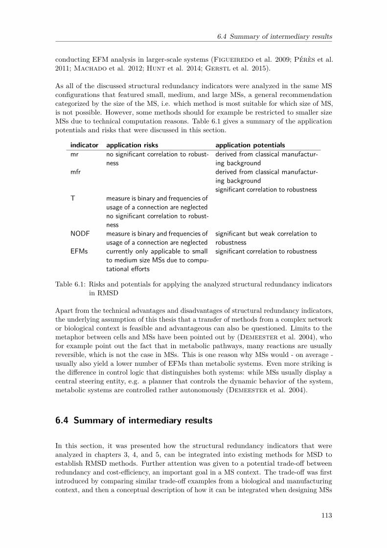
6.4 Summary of intermediary results
conducting EFM analysis in larger-scale systems (Figueiredo et al. 2009; Pérès et al.2011; Machado et al. 2012; Hunt et al. 2014; Gerstl et al. 2015).
As all of the discussed structural redundancy indicators were analyzed in the same MSconfigurations that featured small, medium, and large MSs, a general recommendationcategorized by the size of the MS, i.e. which method is most suitable for which size of MS,is not possible. However, some methods should for example be restricted to smaller sizeMSs due to technical computation reasons. Table 6.1 gives a summary of the applicationpotentials and risks that were discussed in this section.
indicator application risks application potentialsmr no significant correlation to robust-
nessderived from classical manufactur-ing background
mfr derived from classical manufactur-ing backgroundsignificant correlation to robustness
T measure is binary and frequencies ofusage of a connection are neglectedno significant correlation to robust-ness
NODF measure is binary and frequencies ofusage of a connection are neglected
significant but weak correlation torobustness
EFMs currently only applicable to smallto medium size MSs due to compu-tational efforts
significant correlation to robustness
Table 6.1: Risks and potentials for applying the analyzed structural redundancy indicatorsin RMSD
Apart from the technical advantages and disadvantages of structural redundancy indicators,the underlying assumption of this thesis that a transfer of methods from a complex networkor biological context is feasible and advantageous can also be questioned. Limits to themetaphor between cells and MSs have been pointed out by (Demeester et al. 2004), whofor example point out the fact that in metabolic pathways, many reactions are usuallyreversible, which is not the case in MSs. This is one reason why MSs would - on average -usually also yield a lower number of EFMs than metabolic systems. Even more striking isthe difference in control logic that distinguishes both systems: while MSs usually display acentral steering entity, e.g. a planner that controls the dynamic behavior of the system,metabolic systems are controlled rather autonomously (Demeester et al. 2004).
6.4 Summary of intermediary results
In this section, it was presented how the structural redundancy indicators that wereanalyzed in chapters 3, 4, and 5, can be integrated into existing methods for MSD toestablish RMSD methods. Further attention was given to a potential trade-off betweenredundancy and cost-efficiency, an important goal in a MS context. The trade-off was firstintroduced by comparing similar trade-off examples from a biological and manufacturingcontext, and then a conceptual description of how it can be integrated when designing MSs
113

6 Designing robust manufacturing systems with redundancy considerations
with higher robustness was given. Overall, it can be concluded that the aspect of robustnessand cost-efficiency trade-offs should be taken into account by companies when they want toincrease their robustness. A thorough discussion on the advantages and disadvantages ofthe use of structural redundancy indicators in MSD concludes this chapter. In the followingconclusion, an overall summary, assumptions and limitations of the presented works, aswell as implications for industry and research are presented.
114
7 Conclusion
The last chapter of this thesis firstly gives a summary of the overall findings, with referenceto the initial research questions that were set up in chapter 1. It continues with a summaryof the main assumptions and limitations of the chosen methods. Subsequently, implicationsof the thesis findings on industry are given. The chapter finally concludes with an outlookon future research.
7.1 Summary of results
The overarching aim of this thesis was to investigate the role of redundancies as a means toachieve performance robustness in MSs and to integrate such findings into RMSD methods.The guiding research question was split into several sub-questions that were answered inthe different chapters of this thesis, and a summary of each of the findings related to thequestions will be given in the following.
Subquestion 1. How can robustness be defined and measured in manufacturing systems?
In the second chapter, a thorough review of robustness definitions in general and in a MScontext was given (see sections 2.2.1 and 2.2.2). It was found that the majority of existingapproaches concerned with RMSD are so called robust parameter design methods, whichare based on Taguichi methods (see section 2.2.3). Only a small amount of approachesfor RMSD were identified in literature. As robustness is a well-studied characteristic indisciplines such as biology and complex networks science, robustness definitions from thesescientific fields were also included in the review (see sections 2.3.2 and 2.3.3). From theseexisting approaches in literature, a new indicator to measure robustness in MSs, which isbased on the behavior of the MSP measure lateness, was derived to be used within thisthesis in section 3.1.
Subquestion 2. How can redundancy be defined and measured in manufacturing systems?
Similar to the approach for the previous subquestion, an extensive literature review wasconducted in the second chapter to also collect redundancy definitions in general andwith specific relation to a manufacturing context (see section 2.2.5 and 3.2). Whiledifferent approaches to define redundancy exist in biology or complex network science (seesections 2.3.3), it was concluded that no clear definition of redundancy has been establishedin the area of MSs research (see sections 2.2.7 and 2.4). Thus a definition and measuresfor redundancy in MSs based on machine redundancy were derived for further use in thisthesis in section 3.2. In addition to this redundancy measure derived from a classicalmanufacturing background, two indicators for redundancy from a biological background,nestedness and EFMs, were also identified as potential indicators for redundancy in MSs.
115

7 Conclusion
Subquestion 3. How is the relationship between robustness of manufacturing systemperformance and redundancy characterized?
After the definitions for robustness and redundancy in a MS context were established inchapter 2, it was analyzed in chapter 3 whether both constructs exhibit a similar relationshipin MSs as they do in other engineered or natural systems, where robustness is usuallyenhanced by redundancy. To analyze this relationship in a large-scale range of differentMSs, firstly a set of realistic MS configurations was created in section 3.4.2. For theseMS configurations, robustness of the MSP performance measure lateness was measured assuggested in the definition given in section 3.1, using a discrete-event simulation model(see section 3.4.3). Likewise, redundancy of each MS configuration was calculated using onthe one hand the previously established definitions based on machine redundancy and onthe other hand indicators from complex network science. Robustness and redundancy werethen correlated, revealing a significant correlation between robustness of the MSP measurelateness and machine functional redundancy over all analyzed MS configurations, while nosignificant correlation could be found between robustness and the indicators derived fromcomplex network science.
To further analyze the relationship between robustness and redundancy in a MS context,two other indicators for redundancy from a biological context were analyzed in chapters 4and 5. The first indicator, nestedness, is a measure used in mutualistic networks to analyzethe relation between structural aspects and robustness of a system. In order to calculatenestedness in MSs, a modeling approach for depicting MSs as mutualistic networks was firstestablished (see section 4.3). Nestedness was then calculated both in an exemplary realworld case study data set of a job shop MS (see section 4.4), and in the MS configurationsgenerated in section 3.4.2 (see section 4.5). The average nestedness values found for theMSs were significantly lower than those usually found in mutualistic networks. Due to a lowand mostly unsignificant correlation between nestedness and robustness, it was concludedthat nestedness is at this stage not as suitable as a robustness indicator in MSs as othermeasures, such as machine redundancy or EFMs, that were also analyzed within thisthesis.
The second redundancy indicator derived from a biological context, EFMs, and its relation-ship to robustness in MSs were analyzed in chapter 5. Firstly the necessary analogies totransfer the concept of EFMs from metabolic to MSs were drawn in a modeling approach(see section 5.2). EFMs were then calculated in the resource – material flow network of areal world case study data set of a MS (see section 5.3) and in the MS configurations createdin section 3.4.2 (see section 5.4). A correlation analysis conducted in section 5.4 revealedthat out of all redundancy indicators analyzed in this thesis (machine redundancy, complexnetwork indicators, nestedness), both EFM indicators exhibit the strongest correlationcoefficients and significance levels when correlated to robustness in MS. It was thereforeconcluded that EFMs are a suitable predictor for robustness of MS performance and canbe used for incorporating robustness into MS designs.
Subquestion 4. How can redundancy be incorporated in the design and reconfigurationof manufacturing systems in order to increase the robustness of manufacturing systemperformance?
116

7.2 Assumptions and limitations
As a last step, it was investigated in chapter 6 how the redundancy indicators that exhibiteda strong correlation and significance (machine functional redundancy and EFMs) can beapplied in practice in order to design robust MSs. It was in particular elaborated on apotential trade-off between robustness caused by redundancy and cost-efficiency, whichshould be taken into account when trying to increase the robustness of a MS design (seesection 6.2).
Guiding research question. How can redundancies be integrated in manufacturingsystems design so that the manufacturing system performance robustness increases?
To draw an overall summary of the thesis results, the guiding research question can beanswered as follows. It was shown in the course of this research that, for a large range ofdifferent MS configurations, a significant correlation exists between robustness and differentstructural redundancy measures. An especially striking correlation was discovered betweena redundancy indicator used in systems biology and robustness of MSs, confirming thebenefit of applying interdisciplinary methods in MS research. The integration of suchstructural measures can be accomplished by either integrating the structural indicatoras a model variable, or by using it as an assessment criterion of a created MS design.Special attention should however be paid to creating robust designs of MSs, as unfavorabletrade-offs between robustness and other MS targets, such as efficiency, potentially exist.
7.2 Assumptions and limitations
In the following, an overall summary of the assumptions and limitations of the methods usedwithin this research work is given, while it is also elaborated on the generalizability of thefindings. The overarching aim of this thesis was to analyze the relation between robustnessand redundancy in MSs. This research goal can be counted as basic or fundamentalresearch, which is defined as research aimed to improve general knowledge or understandingof phenomena (National Science Foundation 1953). In domains such as biology,phenomena are usually investigated in a large amount of real world data sets, as for exampledone by Bascompte et al. (2003) for plant-pollinator networks, which ensures a strongstatistical significance and generalizability of the findings. However, in a manufacturingcontext, obtaining large-scale data sets from a different range of real MSs is hardly possible.To ensure that the results of this thesis can still be generalized for a large range of differentMSs, the conducted simulation study was thus based on a large-scale amount of differentMS configurations. The MS configurations were created using an optimization model thatcreates cost-optimal layouts, which would be a typical assumption in a manufacturingorganization.
The generalizability of the overall results is also influenced by the simulation model utilizedin section 3.4.3. In the simulation study, only a single breakdown of one machine at a timeis analyzed, meaning that the calculated robustness value only indicates how robust the MSis against single-machine breakdowns. This is sufficient for a first explorative analysis ofthe matter, but to enhance applicability of the results in practice, a more realistic scenariothat depicts robustness against multiple breakdowns would have to be analyzed. Moreover,the underlying dispatching principle used in the simulation model is FIFO, meaning the
117

7 Conclusion
results are transferable for MS that operate with this type of dispatching rule, yet theymight change for other control principles.
To also ensure that the established analogies and modeling approaches for nestedness andEFMs in MSs (see chapters 4 and 5) are not only analyzed in artificially created testinstances of MS configurations, it was also shown that the calculations can be applied totwo case study MSs with real world data (see section 4.4 and 5.3). Hence the approach inthis thesis can be described as a combination of explorative, experimental and case studyresearch.
7.3 Implications for industry
As stated in chapter 6, the insights gained on the relationship between robustness andredundancy can be used by manufacturing organizations during their design or re-designprocess. The structural indicators allow for an easy assessment of the robustness of acompany’s MS, and thus can be seen as an aid for decision making. While on a short termscale increased redundancy in a MS could increase the manufacturing costs, redundancyhelps to buffer against robustness on a rather long term perspective. Increasing redundancyand thus robustness of MSs can be seen as a way of managing uncertainty in MSs, whichis an important aspect in the management of manufacturing organizations for example inthe face of risk analysis (Thun et al. 2011). When structural redundancy indicators areimplemented in methods to create RMSD as suggested in section 6.1, they can thus help toprovide manufacturing managers with a decision-making framework to decide analyticallyfrom among various MS configuration alternatives, for example when making long termkey decisions such as technology selection.
7.4 Outlook on further research
With the analogies and modeling approaches established within this thesis in chapters 4and 5, a calculation of nestedness and EFMs in a manufacturing context was made possiblefor the first time. Based on the modeling approaches presented, structural indicatorslike EFMs can now be integrated into optimization or simulation models to comparethe performance of MSDs that are based on EFMs to the performance of designs thatwere created using standard MSD methods which are usually based on cost-efficiency (seesection 2.1.3). The modeling approaches developed here further provide a basis for theapplication of nestedness and EFM analysis in a MS context also for different researchpurposes apart from research on robustness. A comparison of the structural nestednessor EFM indicators to other structural indicators such as flexibility or complexity, whichare constructs that are of great interest in MS research (see section 2.2.1), is also feasible.Similar to the approach chosen in this thesis, a potential relation between redundancy andother dynamic MSP measures, for example throughput times, is now also possible.
Moreover, the modeling of MSs as metabolic networks also enables the application offurther, very promising methods from the domain of systems biology. With the descriptionof how a MS can be modeled as a stoichiometric matrix of a metabolic network given
118

7.4 Outlook on further research
in section 5.2, other systems biology methods that are based on input data from thestoichiometric matrix of a metabolic network are potentially applicable to a MS context.A very interesting example for this is FBA, which was briefly introduced in section 2.3.3.FBA is an operations research based method formulated for the prediction of metabolicfluxes and often used used to analyze the robustness of metabolic systems (Varma andPalsson 1994; Edwards and Palsson 2000; Orth et al. 2010). As such a model isconceptually very close to the traditional methods used for MSD (see section 2.1.3), thetransfer of FBA to further investigate the robustness of MSP seems extremely promising.
119

Bibliography
Accenture. Keeping ahead of supply chain risk and uncertainty. Tech. rep. 2008.AlGeddawy, T. and H. ElMaraghy. “Co-evolution hypotheses and model for manufac-
turing planning.” In: CIRP Annals - Manufacturing Technology 59.1 (2010), pp. 445–448.doi: 10.1016/j.cirp.2010.03.032.
Albert, Réka and Albert-László Barabási. “Statistical mechanics of complex networks.”In: Reviews of Modern Physics 74.1 (2002), pp. 47–97. doi: 10.1103/RevModPhys.74.47.
Albert, Réka, Hawoong Jeong, and Albert-László Barabási. “Internet: Diameter ofthe World-Wide Web.” In: Nature 401.6749 (1999), pp. 130–131. doi: 10.1038/43601.
– “Error and attack tolerance of complex networks.” In: Nature 406.6794 (2000), pp. 378–382. doi: 10.1038/35019019.
Albert, Réka, István Albert, and Gary L. Nakarado. “Structural vulnerability of theNorth American power grid.” In: Physical Review E - Statistical, Nonlinear, and SoftMatter Physics 69.2 2 (2004), pp. 1–4. doi: 10.1103/PhysRevE.69.025103.
Albert, Réka, Bhaskar DasGupta, Rashmi Hegde, Gowri Sangeetha Sivanathan,Anthony Gitter, Gamze Gürsoy, Pradyut Paul, and Eduardo Sontag. “Computa-tionally efficient measure of topological redundancy of biological and social networks.”In: Physical Review E 84.3 (2011), p. 036117. doi: 10.1103/PhysRevE.84.036117.
Alberts, Bruce, Alexander Johnson, Julian Lewis, Martin Raff, Keith Roberts, andPeter Walter. Molecular Biology of the Cell. 5th ed. Garland Science, 2008.
Albino, V. and a.C. Garavelli. “A methodology for the vulnerability analysis ofjust-in-time production systems.” In: International Journal of Production Economics41.1-3 (1995), pp. 71–80. doi: 10.1016/0925-5273(95)00014-3.
Alderson, D. L. “Catching the "Network Science" Bug: Insight and Opportunity forthe Operations Researcher.” In: Operations Research 56.5 (2008), pp. 1047–1065. doi:10.1287/opre.1080.0606.
Alderson, David L. and John C. Doyle. “Contrasting views of complexity and theirimplications for network-centric infrastructures.” In: IEEE Transactions on Systems,Man, and Cybernetics Part A:Systems and Humans. Vol. 40. 4. 2010, pp. 839–852. doi:10.1109/TSMCA.2010.2048027.
Alhourani, Farouq. “Cellular manufacturing system design considering machines relia-bility and parts alternative process routings.” In: International Journal of ProductionResearch 54.3 (2016), pp. 846–863. doi: 10.1080/00207543.2015.1083626.
Ali, Mohammed and Subhash Wadhwa. “The effect of routing flexibility on a flexiblesystem of integrated manufacturing.” In: International Journal of Production Research48.19 (2010), pp. 5691–5709. doi: 10.1080/00207540903100044.
Almeida-Neto, Mário, Paulo Guimara, Paulo R Guimara, Rafael D Loyola, andWerner Ulrich. “A consistent metric for nestedness analysis in ecological systems :reconciling concept and measurement.” In: Oikos 117.8 (2008), pp. 1227–1240. doi:10.1111/j.2008.0030-1299.
120

Bibliography
Alting, Leo, Arne Bilberg, and Niels Erik Larsen. “Extended Applications of Simulationin Manufacturing Systems.” In: CIRP Annals - Manufacturing Technology 37.1 (1988),pp. 417–420.
Altiok, Tayfur. Performance Analysis of Manufacturing Systems. Springer Science &Business Media, 1997.
Altiok, Tayfur and Benjamin Melamed. Simulation Modeling and Analysis with ARENA.Elsevier Science, 2010.
Araujo, Aderaldo I.L., Adriana M. de Almeida, Márcio Z. Cardoso, and GilbertoCorso. “Abundance and nestedness in interaction networks.” In: Ecological Complexity7.4 (2010), pp. 494–499. doi: 10.1016/j.ecocom.2010.02.004.
Armbruster, Dieter, Pierre Degond, and Christian Ringhofer. “Continuum models forinteracting machines.” In: Networks of Interacting Machines. Ed. by DieterArmbruster,Kunihiko Kaneko, and Alexander S. Mikhailov. World Scientific, 2005, pp. 1–31.
Armbruster, Dieter, P. Degond, and C. Ringhofer. “A Model for the Dynamics oflarge Queuing Networks and Supply Chains.” In: SIAM Journal on Applied Mathematics66.3 (2006), pp. 896–920. doi: 10.1137/040604625.
Askin, Ronald G. “Contributions to the design and analysis of cellular manufacturingsystems.” In: International Journal of Production Research 51.23-24 (2013), pp. 6778–6787. doi: 10.1080/00207543.2013.825745.
Askin, Ronald G. and M.George Mitwasi. “Integrating facility layout with processselection and capacity planning.” In: European Journal of Operational Research 57.2(1992), pp. 162–173. doi: 10.1016/0377-2217(92)90040-G.
Atmar, Wirt and Bruce D. Patterson. “The measure of order and disorder in thedistribution of species in fragmented habitat.” In: Oecologia 96.3 (1993), pp. 373–382.doi: 10.1007/BF00317508.
Azadegan, Arash, Pankaj C. Patel, Abouzar Zangoueinezhad, and Kevin Linderman.“The effect of environmental complexity and environmental dynamism on lean practices.”In: Journal of Operations Management 31.4 (2013), pp. 193–212. doi: 10.1016/j.jom.2013.03.002.
Bahl, Harish C and Larry P Ritzman. “Determining Lot Sizes and Resource Requirements:A Review.” In: Operations Research 35.3 (1987), pp. 329–345.
Baker, Jack W., Matthias Schubert, and Michael H. Faber. “On the assessment ofrobustness.” In: Structural Safety 30 (2008), pp. 253–267. doi: 10.1016/j.strusafe.2006.11.004.
Balci, O. “How to assess the acceptability and credibility of simulation results.” In:Proceedings of the 1989 Winter Simulation Conference. Ed. by E.A. MacNair, K.J.Musselman, and P. Heidelberger. ACM Press, 1989, pp. 62–71. doi: 10.1145/76738.76746.
Balci, Osman. “Guidelines for successful simulation studies.” In: Proceedings of the1990 Winter Simulation Conference. Ed. by Osman Balci, Randall P. Sadowski, andRichard E. Nance. IEEE, 1990, pp. 25–32. doi: 10.1109/WSC.1990.129482.
Baldwin, J S, C. Rose-Anderssen, and K Ridgway. “Linnaean and Cladistic Classifi-cations of Manufacturing Systems.” In: Enabling Manufacturing Competitiveness andEconomic Sustainability. Ed. by H.A. ElMaraghy. Springer, 2012, pp. 28–34. doi:10.1007/978-3-642-23860-4_4.
Bar-Yam, Yaneer. Dynamics of Complex Systems. Addison-Wesley, 1997.Barabási, Albert-László. “The network takeover.” In: Nature Physics 8.1 (2012), pp. 14–16. doi: 10.1038/nphys2188.
121

Bibliography
Barabási, Albert-László and Réka Albert. “Emergence of Scaling in Random Networks.”In: Science 286.5439 (1999), pp. 509–512. doi: 10.1126/science.286.5439.509.
Barabási, Albert-László and Jennifer Frangos. Linked: The New Science Of Networks.Basic Books, 2014.
Barabási, Albert-László and Zoltán N Oltvai. “Network biology: understanding thecell’s functional organization.” In: Nature reviews. Genetics 5.2 (2004), pp. 101–13. doi:10.1038/nrg1272.
Bard, Jonathan F. and Thomas a. Feo. “An Algorithm for the Manufacturing EquipmentSelection Problem.” In: IIE Transactions 23.February 2015 (1991), pp. 83–92. doi:10.1080/07408179108963843.
Barthélemy, M. “Betweenness centrality in large complex networks.” In: EuropeanPhysical Journal B 38.2 (2004), pp. 163–168. doi: 10.1140/epjb/e2004-00111-4.
Bascompte, Jordi and Pedro Jordano. “Plant-Animal Mutualistic Networks: TheArchitecture of Biodiversity.” In: Annual Review of Ecology, Evolution, and Systematics38.1 (2007), pp. 567–593. doi: 10.1146/annurev.ecolsys.38.091206.095818.
– Mutualistic Networks. Princeton University Press, 2013.Bascompte, Jordi, Pedro Jordano, Carlos J Melián, and Jens M Olesen. “Thenested assembly of plant-animal mutualistic networks.” In: Proceedings of the NationalAcademy of Sciences of the United States of America 100.16 (2003), pp. 9383–7. doi:10.1073/pnas.1633576100.
Batterman, Robert W. and Collin C. Rice. “Minimal Model Explanations.” In: Philoso-phy of Science 81.3 (2014), pp. 349–376. doi: 10.1086/676677.
Battini, Daria, Alessandro Persona, and Stefano Allesina. “Towards a use of networkanalysis: quantifying the complexity of Supply Chain Networks.” In: InternationalJournal of Electronic Customer Relationship Management 1.1 (2007), p. 75. doi: 10.1504/IJECRM.2007.014427.
Bebber, Daniel P, Juliet Hynes, Peter R Darrah, Lynne Boddy, and Mark D Fricker.“Biological solutions to transport network design.” In: Proceedings. Biological sciences /The Royal Society 274.1623 (2007), pp. 2307–15. doi: 10.1098/rspb.2007.0459.
Becker, Till and Mirja Meyer. “Performance and Time Based Robustness Measures forDynamical and Multi-variant Manufacturing Systems.” In: Proceedings of the 18th Cam-bridge International Manufacturing Symposium. Institute for Manufacturing, Universityof Cambridge, 2014, pp. 615–626.
Becker, Till, Moritz Emanuel Beber, Katja Windt, Marc-Thorsten Hütt, and DirkHelbing. “Flow control by periodic devices: a unifying language for the description oftraffic, production, and metabolic systems.” In: Journal of Statistical Mechanics: Theoryand Experiment 2011.05 (2011), P05004. doi: 10.1088/1742-5468/2011/05/P05004.
Becker, Till, Mirja Meyer, Moritz Beber, Katja Windt, and Marc-Thorsten Hütt.“A comparison of network characteristics in metabolic and manufacturing systems.” In:Dynamics in Logistics - 3rd International Conference on Dynamics in Logistics (LDIC2012). Ed. by Hans-Jörg Kreowski, Bernd Scholz-Reiter, and Klaus-Dieter Thoben.Springer, 2012, pp. 141–150.
Becker, Till, MirjaMeyer, and KatjaWindt. “A network theory approach for robustnessmeasurement in dynamic manufacturing systems.” In: Disruptive supply network modelsin future industrial systems: configuring for resilience and sustainability. SymposiumProceedings. Institute for Manufacturing, University of Cambridge, 2013.
– “A manufacturing systems network model for the evaluation of complex manufacturingsystems.” In: International Journal of Productivity and Performance Management 63.3(2014), pp. 324–340. doi: 10.1108/IJPPM-03-2013-0047.
122

Bibliography
Behre, Jörn, Thomas Wilhelm, Axel von Kamp, Eytan Ruppin, and Stefan Schuster.“Structural robustness of metabolic networks with respect to multiple knockouts.” In:Journal of Theoretical Biology 252.3 (2008), pp. 433–41. doi: 10.1016/j.jtbi.2007.09.043.
Bellamy, Marcus A. and Rahul C. Basole. “Network analysis of supply chain systems: Asystematic review and future research.” In: Systems Engineering 16.2 (2013), pp. 235–249.doi: 10.1002/sys.21238.
Bellgran, Monica and Eva Kristina Säfsten. Production Development: Design andOperation of Production Systems. 3rd editio. Springer Science & Business Media, 2009.
Benjaafar, Saif, Sunderesh S Heragu, and Shahrukh A Irani. “Next GenerationFactory Layouts: Research Challenges and Recent Progress.” In: Interfaces 32.6 (2002),pp. 58–76.
Bertalanffy, Ludwig Von. General System Theory: Foundations, Development, Applica-tions. Braziller, 2003.
Beyer, Hans-Georg and Bernhard Sendhoff. “Robust optimization – A comprehensivesurvey.” In: Computer Methods in Applied Mechanics and Engineering 196.33-34 (2007),pp. 3190–3218. doi: 10.1016/j.cma.2007.03.003.
Beygelzimer, Alina, Geoffrey Grinstein, Ralph Linsker, and Irina Rish. “Improvingnetwork robustness by edge modification.” In: Physica A: Statistical Mechanics and itsApplications 357 (2005), pp. 593–612. doi: 10.1016/j.physa.2005.03.040.
Bhamra, Ran, Samir Dani, and Kevin Burnard. “Resilience: the concept, a literaturereview and future directions.” In: International Journal of Production Research 49.18(2011), pp. 5375–5393. doi: 10.1080/00207543.2011.563826.
Bhatia, Gurpriya, Charles Lane, and Adrian Wain. Building Resilience in Supply Chains.Accenture, 2013.
Bititci, Umit S. “Modelling of performance measurement systems in manufacturingenterprises.” In: International Journal of Production Economics 42 (1995), pp. 137–147.
Bitran, Gabriel R. and Sriram Dasu. “A review of open queueing network modelsof manufacturing systems.” In: Queueing Systems 12.1-2 (1992), pp. 95–133. doi:10.1007/BF01158637.
Bitran, Gabriel R and Reinaldo Morabito. “An overview of tradeoff curves in manufac-turing system design.” In: Production and Operations Management 8.1 (1999), pp. 56–75.
Bitran, Gabriel R and Devanath Tirupati. “Capacity planning in manufacturing networkswith discrete options.” In: Annals of Operations Research 17.1 (1989), pp. 119–136.
Bitran, Gabriel R. and Devanath Tirupati. “Tradeoff Curves, Targeting and Balancingin Manufacturing Queueing Networks.” In: Operations Research 37.4 (1989), pp. 547–564.
Black, J. Temple. The design of the factory with a future. McGraw-Hill, 1991.Blackstone, John H., Don T. Phillips, and Gary L. Hogg. “A state-of-the-art survey
of dispatching rules for manufacturing job shop operations.” In: International Journal ofProduction Research 20.1 (1982), pp. 27–45. doi: 10.1080/00207548208947745.
Blischke, Wallace R. and D.N. Prabhakar Murthy. Reliability: modeling, prediction,and optimization. John Wiley & Sons, 2011.
Blunck, Henning, Victor Vican, Till Becker, and Katja Windt. “Improvement Heuris-tics for Manufacturing System Design Using Complex Network Figures.” In: ProcediaCIRP 17 (2014), pp. 50–55. doi: 10.1016/j.procir.2014.01.063.
Boccaletti, S, V Latora, Y Moreno, M Chavez, and D Hwang. “Complex networks:Structure and dynamics.” In: Physics Reports 424.4-5 (2006), pp. 175–308. doi: 10.1016/j.physrep.2005.10.009.
123

Bibliography
Bollobas, Bela. Modern Graph Theory. Springer Science & Business Media, 1998.Bollobás, Béla. Random Graphs. Cambridge University Press, 2001.Bollobás, Béla and Oliver Riordan. “Robustness and Vulnerability of Scale-Free Random
Graphs.” In: Internet Mathematics 1.1 (2004), pp. 1–35. doi: 10.1080/15427951.2004.10129080.
Bonabeau, Eric, Marco Dorigo, and Guy Theraulaz. Swarm Intelligence: FromNatural to Artificial Systems. Oxford University Press, 1999.
Bortolotti, Thomas, Pamela Danese, and Pietro Romano. “Assessing the impactof just-in-time on operational performance at varying degrees of repetitiveness.” In:International Journal of Production Research 51.4 (2012), pp. 1–14. doi: 10.1080/00207543.2012.678403.
Boysen, Nils, Simon Emde, Michael Hoeck, and Markus Kauderer. “Part logistics inthe automotive industry: Decision problems, literature review and research agenda.” In:European Journal of Operational Research 242.1 (2015), pp. 107–120. doi: 10.1016/j.ejor.2014.09.065.
Bozarth, Cecil C., Donald P. Warsing, Barbara B. Flynn, and E. James Flynn. “Theimpact of supply chain complexity on manufacturing plant performance.” In: Journal ofOperations Management 27.1 (2009), pp. 78–93. doi: 10.1016/j.jom.2008.07.003.
Braess, D. “Über ein Paradoxon aus der Verkehrsplanung.” In: Operations Research 12.1(1968), pp. 258–268. doi: 10.1007/BF01918335.
Braha, Dan. “The topology and dynamics of complex man- made systems.” In: 2007IEEE International Conference on Systems, Man and Cybernetics (2007), pp. 4062–4068.doi: 10.1109/ICSMC.2007.4414261.
Braha, Dan and Yaneer Bar-Yam. “From centrality to temporary fame: Dynamiccentrality in complex networks.” In: Complexity 12.2 (2006), pp. 59–63. doi: 10.1002/cplx.20156.
Brandimarte, Paolo. “Routing and scheduling in a flexible job shop by tabu search.” In:Annals of Operations Research 41.3 (1993), pp. 157–183. doi: 10.1007/BF02023073.
Brandimarte, Paolo and Agostino Villa. Advanced Models for Manufacturing SystemsManagement. CRC Press, 1995.
Brandon-Jones, Emma, Brian Squire, and Yvonne G.T. Van Rossenberg. “Theimpact of supply base complexity on disruptions and performance: the moderating effectsof slack and visibility.” In: International Journal of Production Research (2014), pp. 1–16.doi: 10.1080/00207543.2014.986296.
Brintrup, Alexandra, Yu Wang, and Ashutosh Tiwari. “Supply Networks as ComplexSystems: A Network-Science-Based Characterization.” In: IEEE Systems Journal (2015),pp. 1–12. doi: 10.1109/JSYST.2015.2425137.
Burgos, Enrique, Horacio Ceva, R. P J Perazzo, Mariano Devoto, Diego Medan,Martín Zimmermann, and Ana María Delbue. “Why nestedness in mutualisticnetworks?” In: Journal of Theoretical Biology 249.2 (2007), pp. 307–313. doi: 10.1016/j.jtbi.2007.07.030.
Buzacott, John A and J. George Shanthikumar. “Design of manufacturing systemsusing queueing models.” In: Queueing Systems 12.1-2 (1992), pp. 135–213. doi: 10.1007/BF01158638.
Buzacott, John a. “The Effect of Station Breakdowns and Random Processing Timeson the Capacity of Flow Lines with In-Process Storage.” In: A I I E Transactions 4.4(1972), pp. 308–312. doi: 10.1080/05695557208974867.
CIRP, ed. Dictionary of Production Engineering Vol. 3 - Manufacturing Systems. Springer,2004.
124

Bibliography
Caggiano, Allessandra. “Manufacturing System.” In: CIRP Encyclopedia of ProductionEngineering. Ed. by Luc Laperrière and Gunther Reinhart. Springer, 2014, pp. 830–836. doi: 10.1007/978-3-642-20617-7_6562.
Calinescu, A., J. Efstathiou, J. Schirn, and J. Bermejo. “Applying and AssessingTwo Methods for Measuring Complexity in Manufacturing.” In: The Journal of theOperational Research Society 49.7 (1998), pp. 723–733. doi: 10.2307/3010243.
Callaway, D S, M E Newman, S H Strogatz, and D J Watts. “Network robustnessand fragility: percolation on random graphs.” In: Physical review letters 85.25 (2000),pp. 5468–71.
Caprihan, Rahul and Subhash Wadhwa. “Impact of Routing Flexibility on the Perfor-mance of an FMS—A Simulation Study.” In: International Journal of Flexible Manufac-turing Systems 9.3 (1997), pp. 273–298. doi: 10.1023/A:1007917429815.
Carrie, Allan S, James M Moore, Marek Roczniak, and Jouko J Seppänen. “Graphtheory and computer aided facilities design.” In: Omega 6.4 (1978), pp. 353–361. doi:10.1016/0305-0483(78)90008-7.
Carson, John S. “Model verification and validation.” In: Proceedings of the 2002 WinterSimulation Conference. Ed. by E. Yücesan, C.-H. Chen, J.L. Snowdown, and J.M.Charnes. Vol. 1. IEEE, 2002, pp. 52–58. doi: 10.1109/WSC.2002.1172868.
Ceryan, O. and Yoram Koren. “Manufacturing capacity planning strategies.” In: CIRPAnnals - Manufacturing Technology 58.1 (2009), pp. 403–406. doi: 10.1016/j.cirp.2009.03.034.
Chan, Felix T. S. “The effects of routing flexibility on a flexible manufacturing system.” In:International Journal of Computer Integrated Manufacturing 14.5 (2001), pp. 431–445.doi: 10.1080/09591120010021793.
Chance, Frank, Jennifer Robinson, and John W. Fowler. “Supporting manufacturingwith simulation.” In: Proceedings of the 28th conference on Winter simulation - WSC’96. New York, New York, USA: ACM Press, 1996, pp. 114–121. doi: 10.1145/256562.256586.
Chandrasekharan, M.P. and R. Rajagopalan. “An ideal seed non-hierarchicalclustering algorithm for cellular manufacturing.” In: International Journal of ProductionResearch 24.2 (1986), pp. 451–463. doi: 10.1080/00207548608919741.
Chapman, J. L. and M. J. Reiss. Ecology: Principles and Applications. CambridgeUniversity Press, 1999.
Checkland, Peter. Systems thinking, systems practice. 2nd ed. John Wiley, 1999.Chen, Chin-Fu. “Review on Robustness in Systems Biology.” In: Journal of Biomecha-tronics Engineering 1.2 (2008), pp. 17–28.
Chen, K. S. and M. L. Huang. “Performance measurement for a manufacturing systembased on quality, cost and time.” In: International Journal of Production Research 44(2006), pp. 2221–2243. doi: 10.1080/00207540500446360.
Chen, M. “A heuristic for solving manufacturing process and equipment selection prob-lems.” In: International Journal of Production Research 37.2 (1999), pp. 359–374. doi:10.1080/002075499191814.
Chen, Wei, J.K. Allen, Kwok-Leung Tsui, and F. Mistree. “A procedure for robustdesign: minimizing variations caused by noise factors and control factors.” In: Journalof Mechanical Design 118.4 (1996), pp. 478–485.
Chiang, Wen-Chyuan, Timothy L. Urban, JianQiang Hu, Hongyu Li, Yifan Xu, andShanling Li. “Interdisciplinary research in operations management.” In: InternationalJournal of Production Economics 147 (2014), pp. 571–572. doi: 10.1016/j.ijpe.2013.11.013.
125

Bibliography
Chong, Chin Soon, Appa Iyer Sivakumar, Malcolm Yoke Hean Low, and Kheng LengGay. “A bee colony optimization algorithm to job shop scheduling.” In: Proceedingsof the 38th conference on Winter simulation. Winter Simulation Conference, 2006,pp. 1954–1961.
Chryssolouris, George. Manufacturing Systems: Theory and Practice: Theory andPractice. Springer, 2006.
Chryssolouris, George, Konstantinos Efthymiou, Nikolaos Papakostas, DimitrisMourtzis, and Aris Pagoropoulos. “Flexibility and complexity: is it a trade-off?”In: International Journal of Production Research 51.23-24 (2013), pp. 6788–6802. doi:10.1080/00207543.2012.761362.
Chtourou, Hédi, Wassim Masmoudi, and Aref Maalej. “An expert system for manu-facturing systems machine selection.” In: Expert Systems with Applications 28.3 (2005),pp. 461–467. doi: 10.1016/j.eswa.2004.12.007.
Cochran, David S., Jorge F. Arinez, James W. Duda, and Joachim Linck. “Adecomposition approach for manufacturing system design.” In: Journal of ManufacturingSystems 20.6 (2001), pp. 371–389. doi: 10.1016/S0278-6125(01)80058-3.
Cohen, Reuven and Shlomo Havlin. Complex Networks: Structure, Robustness andFunction. Cambridge University Press, 2010.
Connel, Joseph H. and Wayne P. Sousa. “On the evidence needed to judge ecologicalstability or persistence.” In: The American Naturalist 121.6 (1983), pp. 789–824.
Cook, Thomas. “Managing Global Supply Chains.” In: McKinsey Quarterly July (2008),pp. 1–9. doi: 10.1201/9781420064582.
Cotgreave, Peter and Irwin Forseth. Introductory Ecology. Blackwell Sciene, 2002.Crowson, Richard. Factory Operations: Planning and Instructional Methods. Taylor andFrancis, 2005.
Curry, Guy L. and Richard M. Feldman. Manufacturing Systems Modeling and Analysis.Springer, 2010.
Cutler, Alan H. “Nested biotas and biological conservation: metrics, mechanisms, andmeaning of nestedness.” In: Landscape and Urban Planning 28.1 (1994), pp. 73–82. doi:10.1016/0169-2046(94)90045-0.
Da Silveira, Giovani. “Improving trade-offs in manufacturing: Method and illustration.”In: International Journal of Production Economics 95.1 (2005), pp. 27–38. doi: 10.1016/j.ijpe.2003.10.023.
Da Silveira, Giovani and Nigel Slack. “Exploring the trade-off concept.” In: InternationalJournal of Operations & Production Management 21.7 (2001), pp. 949–964. doi: 10.1108/01443570110393432.
Dagdeviren, Metin. “Decision making in equipment selection: An integrated approachwith AHP and PROMETHEE.” In: Journal of Intelligent Manufacturing 19.4 (2008),pp. 397–406. doi: 10.1007/s10845-008-0091-7.
Das, Sanchoy K. and P. Nagendra. “Investigations into the impact of flexibility onmanufacturing performance.” In: International Journal of Production Research 31.10(1993), pp. 2337–2354. doi: 10.1080/00207549308956861.
Das, Sanchoy K. and Prashanth Nagendra. “Selection of routes in a flexible manufactur-ing facility.” In: International Journal of Production Economics 48.3 (1997), pp. 237–247.doi: 10.1016/S0925-5273(96)00106-5.
Dashchenko, Anatoli I., ed. Reconfigurable Manufacturing Systems and TransformableFactories. Springer Science & Business Media, 2007.
126

Bibliography
Davis, R P and D M Miller. “A model for determining machine reqiurements ina multistage manufacturing system with discretely distributed demand.” In: AppliedMathematical Modelling 2.2 (1978), pp. 119–122.
Davis, Robert P, Marvin H Agee, Jose M.A. Tanchoco, and Richard A. Wysk. “Man-ufacturing systems planning.” In: Engineering Management International 3.4 (1986),pp. 231–236. doi: 10.1016/0167-5419(86)90018-9.
DeGarmo, Ernest P., J. T. Black, and Ronald A. Kohser. DeGarmo’s Materials andProcesses in Manufacturing. 11th ed. John Wiley & Sons, 2011.
Dellino, Gabriella, Jack P.C. Kleijnen, and Carlo Meloni. “Robust optimization insimulation: Taguchi and Response Surface Methodology.” In: International Journal ofProduction Economics 125.1 (2010), pp. 52–59. doi: 10.1016/j.ijpe.2009.12.003.
Deloitte. Age of disruption - Are Canadian firms prepared? Tech. rep. 2015.Demeester, Lieven, Knut Eichler, and Christoph H. Loch. “Organic Production Sys-
tems: What the Biological Cell Can Teach Us About Manufacturing.” In: Manufacturing& Service Operations Management 6.2 (2004), pp. 115–132. doi: 10.1287/msom.1030.0033.
Deshmukh, Abhijit V., Joseph J. Talavage, and Moshe M. Barash. “Complexity inmanufacturing systems, Part 1: Analysis of static complexity.” In: IIE Transactions 30.7(1998), pp. 645–655. doi: 10.1080/07408179808966508.
Diestel, Reinhard. Graph Theory. Springer, 2012.Dorigo, M and L M Gambardella. “Ant colonies for the travelling salesman problem.”In: Bio Systems 43.2 (1997), pp. 73–81. doi: 10.1016/S0303-2647(97)01708-5.
Dorigo, M, V Maniezzo, and a Colorni. “The ant systems: optimization by a colonyof cooperative agents.” In: IEEE Transactions on Man, Machine and Cybernetics-PartB 26.1 (1996).
Dou, Bing Lin, Xue Guang Wang, and Shi Yong Zhang. “Robustness of networks againstcascading failures.” In: Physica A: Statistical Mechanics and its Applications 389.11(2010), pp. 2310–2317. doi: 10.1016/j.physa.2010.02.002.
Dovich, Robert A. Reliability Statistics. ASQC Quality Press, 1990.Drucker, Peter. The Practice of Management. 2nd ed. Routledge, 2011.Dunne, Ja, Rj Williams, and Nd Martinez. “Network structure and robustness ofmarine food webs.” In: Marine Ecology Progress Series 273 (2004), pp. 291–302. doi:10.3354/meps273291.
Dunne, Jennifer A, Richard J Williams, and Neo D Martinez. “Food-web structureand network theory: The role of connectance and size.” In: Proceedings of the NationalAcademy of Sciences 99.20 (2002), pp. 12917–12922. doi: 10.1073/pnas.192407699.
Dunne, Jennifer a., Richard J. Williams, and Neo D. Martinez. “Network structureand biodiversity loss in food webs: robustness increases with connectance.” In: EcologyLetters 5.4 (2002), pp. 558–567. doi: 10.1046/j.1461-0248.2002.00354.x.
Edelman, G M and J a Gally. “Degeneracy and complexity in biological systems.” In:Proceedings of the National Academy of Sciences of the United States of America 98.24(2001), pp. 13763–13768. doi: 10.1073/pnas.231499798.
Edwards, J S and B O Palsson. “Robustness analysis of the Escherichia coli metabolicnetwork.” In: Biotechnology progress 16.6 (2000), pp. 927–39. doi: 10.1021/bp0000712.
Edwards, J S, R U Ibarra, and B O Palsson. “In silico predictions of Escherichia colimetabolic capabilities are consistent with experimental data.” In: Nature biotechnology19.2 (2001), pp. 125–130. doi: 10.1038/84379.
127

Bibliography
Efthymiou, K., a. Pagoropoulos, N. Papakostas, D. Mourtzis, and G. Chrys-solouris. “Manufacturing systems complexity review: Challenges and outlook.” In:Procedia CIRP 3 (2012), pp. 644–649. doi: 10.1016/j.procir.2012.07.110.
Eilon, Samuel and I.G. Chowdhury. “Due dates in job shop scheduling.” In: Inter-national Journal of Production Research 14.2 (1976), pp. 223–237. doi: 10.1080/00207547608956596.
ElMaraghy, H., T. AlGeddawy, S.N. Samy, and V. Espinoza. “A model for assessingthe layout structural complexity of manufacturing systems.” In: Journal of ManufacturingSystems 33.1 (2014), pp. 51–64. doi: 10.1016/j.jmsy.2013.05.012.
ElMaraghy, Hoda A, ed. Changeable and Reconfigurable Manufacturing Systems.Springer Science & Business Media, 2008.
ElMaraghy, Hoda, Tarek AlGeddawy, and Ahmed Azab. “Modelling evolution inmanufacturing: A biological analogy.” In: CIRP Annals - Manufacturing Technology57.1 (2008), pp. 467–472. doi: 10.1016/j.cirp.2008.03.136.
ElMaraghy, Waguih, Hoda ElMaraghy, Tetsuo Tomiyama, and Laszlo Monostori.“Complexity in engineering design and manufacturing.” In: CIRP Annals - ManufacturingTechnology 61.2 (2012), pp. 793–814. doi: 10.1016/j.cirp.2012.05.001.
Emami-Mehrgani, Behnam, Sylvie Nadeau, and Jean Pierre Kenné. “Lockout/tagoutand operational risks in the production control of manufacturing systems with passiveredundancy.” In: International Journal of Production Economics 132 (2011), pp. 165–173.doi: 10.1016/j.ijpe.2011.03.028.
Ermann, Leonardo and D.L. Shepelyansky. “Ecological analysis of world trade.” In:Physics Letters A 377.3-4 (2013), pp. 250–256. doi: 10.1016/j.physleta.2012.10.056.
Eroglu, Cuneyt and ChristianHofer. “Lean, leaner, too lean? The inventory-performancelink revisited.” In: Journal of Operations Management 29.4 (2011), pp. 356–369. doi:10.1016/j.jom.2010.05.002.
Estrada, Ernesto and Juan A. Rodríguez-Velázquez. “Subgraph centrality in complexnetworks.” In: Physical Review E 71.5 (2005), pp. 056103–1 –056103–9. doi: 10.1103/PhysRevE.71.056103.
Farhoodi, F. “A knowledge-based approach to dynamic job-shop scheduling.” In: In-ternational Journal of Computer Integrated Manufacturing 3.2 (1990), pp. 84–95. doi:10.1080/09511929008944436.
Félix, M-a and a Wagner. “Robustness and evolution: concepts, insights and challengesfrom a developmental model system.” In: Heredity 100 (2008), pp. 132–140. doi:10.1038/sj.hdy.6800915.
Feyzioğlu, O., H. Pierreval, and D. Deflandre. “A simulation-based optimization ap-proach to size manufacturing systems.” In: International Journal of Production Research43.2 (2005), pp. 247–266. doi: 10.1080/0020754042000264617.
Figueiredo, Luis F. de, Adam Podhorski, Angel Rubio, Christoph Kaleta, JohnE. Beasley, Stefan Schuster, and Francisco J. Planes. “Computing the shortestelementary flux modes in genome-scale metabolic networks.” In: Bioinformatics 25.23(2009), pp. 3158–3165. doi: 10.1093/bioinformatics/btp564.
Fischer, Eliane and Uwe Sauer. “Metabolic flux profiling of Escherichia coli mutants incentral carbon metabolism using GC-MS.” In: European Journal of Biochemistry 270.5(2003), pp. 880–891. doi: 10.1046/j.1432-1033.2003.03448.x.
Fortuna, Miguel A. and Jordi Bascompte. “Habitat loss and the structure of plant-animal mutualistic networks.” In: Ecology Letters 9.3 (2006), pp. 281–286. doi: 10.1111/j.1461-0248.2005.00868.x.
128

Bibliography
Foulds, L. R. and D. F. Robinson. “Graph theoretic heuristics for the plant layoutproblem.” In: International Journal of Production Research 16.1 (1978), pp. 27–37. doi:10.1080/00207547808929997.
Fowler, J. W. “Grand Challenges in Modeling and Simulation of Complex ManufacturingSystems.” In: Simulation 80.9 (2004), pp. 469–476. doi: 10.1177/0037549704044324.
Fox Keller, Evelyn. “Revisiting “scale-free” networks.” In: BioEssays 27.10 (2005),pp. 1060–1068. doi: 10.1002/bies.20294.
Framinan, Jose M., Rainer Leisten, and Rubén Ruiz García. Manufacturing SchedulingSystems. Springer, 2014. doi: 10.1007/978-1-4471-6272-8.
Freeman, Linton C. “A Set of Measures of Centrality Based on Betweenness.” In: So-ciometry 40.1 (1977), pp. 35–41. doi: 10.2307/3033543.
Frizelle, G. and E. Woodcock. “Measuring complexity as an aid to developingoperational strategy.” In: International Journal of Operations & Production Management15.5 (1995), pp. 26–39. doi: 10.1108/01443579510083640.
Frizelle, G, D McFarlane, and L Bongaerts. “Disturbance Measurement in Manu-facturing Production Systems.” In: Proceedings of ASI 98 (1998), pp. 1–12.
Fulkerson, B. and V. Parunak. “The living factory: applications of artificial lifeto manufacturing.” In: Proceedings ISADS 95. Second International Symposium onAutonomous Decentralized Systems. IEEE Comput. Soc. Press, 1995, pp. 391–397. doi:10.1109/ISADS.1995.398998.
Gershwin, S. B. Manufacturing Systems Engineering. PTR Prentice Hall, 1994.Gerstl, Matthias P., David E. Ruckerbauer, Diethard Mattanovich, ChristianJungreuthmayer, and Jürgen Zanghellini. “Metabolomics integrated elementaryflux mode analysis in large metabolic networks.” In: Scientific Reports 5.8930 (2015),pp. 1–8. doi: 10.1038/srep08930.
Ghalayini, Alaa M., James S. Noble, and Thomas J. Crowe. “An integrated dynamicperformance measurement system for improving manufacturing competitiveness.” In:International Journal of Production Economics 48 (1997), pp. 207–225. doi: 10.1016/S0925-5273(96)00093-X.
Goerner, Sally J., Bernard Lietaer, and Robert E. Ulanowicz. “Quantifying economicsustainability: Implications for free-enterprise theory, policy and practice.” In: EcologicalEconomics 69.1 (2009), pp. 76–81. doi: 10.1016/j.ecolecon.2009.07.018.
Goh, K-I, E Oh, B Kahng, and D Kim. “Betweenness centrality correlation in socialnetworks.” In: Physical Review E 67.1 (2003), p. 017101. doi: 10.1103/PhysRevE.67.017101.
Gomes, Carlos F., Mahmoud M. Yasin, and João V. Lisboa. “A literature review ofmanufacturing performance measures and measurement in an organizational context: aframework and direction for future research.” In: Journal of Manufacturing TechnologyManagement 15.6 (2004), pp. 511–530. doi: 10.1108/17410380410547906.
– “Performance measurement practices in manufacturing firms: an empirical investigation.”In: Journal of Manufacturing Technology Management 17 (2006), pp. 144–167. doi:10.1108/17410380610642241.
Gopalakrishnan, B., T. Yoshii, and S.M. Dappili. “Decision support system formachining center selection.” In: Journal of Manufacturing Technology Management 15.2(2004), pp. 144–154. doi: 10.1108/09576060410513733.
Gordon, Robert. “Optimum component redundancy for maximum system reliability.” In:Operations Research 5.2 (1957), pp. 229–243.
129

Bibliography
Gordon, Valery, Jean-Marie Proth, and Chengbin Chu. “A survey of the state-of-the-art of common due date assignment and scheduling research.” In: European Journal ofOperational Research 139.1 (2002), pp. 1–25. doi: 10.1016/S0377-2217(01)00181-3.
Goren, Selcuk and Ihsan Sabuncuoglu. “Robustness and stability measures for schedul-ing: single-machine environment.” In: IIE Transactions 40.1 (2008), pp. 66–83. doi:10.1080/07408170701283198.
– “Optimization of schedule robustness and stability under random machine breakdownsand processing time variability.” In: IIE Transactions 42.3 (2010), pp. 203–220. doi:10.1080/07408170903171035.
Govil, MK and MC Fu. “Queueing theory in manufacturing: A survey.” In: Journal ofManufacturing Systems 18.3 (1999), pp. 214–240.
Gross, Donald, John F. Shortle, James M. Thompson, and Carl M. Harris. Funda-mentals of queueing theory. 4th ed. John Wiley & Sons, 2008.
Gross, Jonathan L., Jay Yellen, and Ping Zhang, eds. Handbook of Graph Theory.2nd ed. CRC Press, 2013.
Guide, V. D. R. and R. Srivastava. “A review of techniques for buffering againstuncertainty with MRP systems.” In: Production Planning & Control 11.3 (2000), pp. 223–233. doi: 10.1080/095372800232199.
Guimaraes Jr., P. R., Victor Rico-Gray, S. Furtado dos Reis, and John N Thompson.“Asymmetries in specialization in ant-plant mutualistic networks.” In: Proceedings of theRoyal Society B: Biological Sciences 273.1597 (2006), pp. 2041–2047. doi: 10.1098/rspb.2006.3548.
Guimaraes Jr., P. R, Cristina Sazima, S. Furtado dos Reis, and I. Sazima. “Thenested structure of marine cleaning symbiosis: is it like flowers and bees?” In: BiologyLetters 3.1 (2007), pp. 51–54. doi: 10.1098/rsbl.2006.0562.
Guimaraes Jr., P.R. and P. Guimaraes. “Improving the analyses of nestedness for largesets of matrices.” In: Environmental Modelling & Software 21.10 (2006), pp. 1512–1513.doi: 10.1016/j.envsoft.2006.04.002.
Guimaraes, Tor, Nils Martensson, Johan Stahre, and Magid Igbaria. “Empiricallytesting the impact of manufacturing system complexity on performance.” In: InternationalJournal of Operations & Production Management 19 (1999), pp. 1254–1269. doi: 10.1108/01443579910294228.
Guldogan, Evrim Ursavas. “An integrated approach to machine selection and operationallocation problem.” In: International Journal of Advanced Manufacturing Technology55.5-8 (2011), pp. 797–805. doi: 10.1007/s00170-010-3063-y.
Gutenberg, Erich. Grundlagen der Betriebswirtschaftslehre - Erster Band - Die Produk-tion. 24th ed. 1983.
Han, Jihee and KwangSup Shin. “Evaluation mechanism for structural robustness ofsupply chain considering disruption propagation.” In: International Journal of ProductionResearch August (2015), pp. 1–17. doi: 10.1080/00207543.2015.1047977.
Hani, Y., L. Amodeo, F. Yalaoui, and H. Chen. “Ant colony optimization for solving anindustrial layout problem.” In: European Journal of Operational Research 183.2 (2007),pp. 633–642. doi: 10.1016/j.ejor.2006.10.032.
Hassan, Mohsen Md and Gary L Hogg. “A review of graph theory application to thefacilities layout problem.” In: Omega 15.4 (1987), pp. 291–300. doi: 10.1016/0305-0483(87)90017-X.
Hayes, Glenn M., Robert P Davis, and Richard A Wysk. “A Dynamic ProgrammingApproach to Machine Requirements Planning.” In: AIIE Transactions 13.2 (1981),pp. 175–181. doi: 10.1080/05695558108974550.
130

Bibliography
Hayes, R H and S C Wheelwright. “Link Manufacturing Process and Product LifeCycles.” In: Harvard Business Review 57.1 (1979), pp. 133–141.
Hayes, Robert H. and Steven C. Wheelwright. Restoring Our Competitive Edge:Competing Through Manufacturing. Wiley, 1984, p. 427.
Hearnshaw, Edward J.S. and Mark M.J. Wilson. “A complex network approach tosupply chain network theory.” In: International Journal of Operations & ProductionManagement 33.4 (2013), pp. 442–469. doi: 10.1108/01443571311307343.
Heim, Gregory R, David Xiaosong Peng, and Shekhar Jayanthi. “Longitudinal Analysisof Inhibitors of Manufacturer Delivery Performance.” In: Decision Sciences 45.6 (2014),pp. 1117–1158.
Helbing, Dirk, Andreas Deutsch, Stefan Diez, Karsten Peters, Yannis Kalaidzidis,Kathrin Padberg-gehle, Anders Johansson, Georg Breier, Stefan L Ammer, FrankSchulze, and Marino Zerial. “Biologistics and the struggle for efficiency.” In: Advancesin Complex Systems 12.6 (2009), pp. 533–548.
Henriet, Fanny, Stéphane Hallegatte, and Lionel Tabourier. “Firm-network char-acteristics and economic robustness to natural disasters.” In: Journal of EconomicDynamics and Control 36.1 (2012), pp. 150–167. doi: 10.1016/j.jedc.2011.10.001.
Heragu, Sunderesh S. Facilities Design. CRC Press/Taylor & Francis Group, 2006.Hill, Arthur V. The Encyclopedia of Operations Management: A Field Manual andGlossary of Operations Management Terms and Concepts. FT Press, 2012.
Hillier, Frederick S. and Kut C. So. “The effect of machine breakdowns and interstagestorage on the performance of production line systems.” In: International Journal ofProduction Research 29.10 (1991), pp. 2043–2055. doi: 10.1080/00207549108948066.
Hitomi, Katsundo. Manufacturing Systems Engineering: A Unified Approach to Manu-facturing Technology, Production Management and Industrial Economics. CRC Press,1996.
Hofer, Christian, Cuneyt Eroglu, and Adriana Rossiter Hofer. “The effect oflean production on financial performance: The mediating role of inventory leanness.”In: International Journal of Production Economics 138.2 (2012), pp. 242–253. doi:10.1016/j.ijpe.2012.03.025.
Holst, Lars. “Integrating Discrete-Event Simulation into the Manufacturing SystemDevelopment Process.” PhD thesis. Lund University, 2001.
Hon, K. K. B. “Performance and Evaluation of Manufacturing Systems.” In: CIRPAnnals - Manufacturing Technology 54.2 (2005), pp. 139–154. doi: 10.1016/S0007-8506(07)60023-7.
Hopp, W.J. and M.L. Spearman. Factory Physics. 3rd ed. McGraw-Hill Education,2008.
Hu, S.J., X. Zhu, H. Wang, and Yoram Koren. “Product variety and manufacturingcomplexity in assembly systems and supply chains.” In: CIRP Annals - ManufacturingTechnology 57.1 (2008), pp. 45–48. doi: 10.1016/j.cirp.2008.03.138.
Hunt, Kristopher a., James P. Folsom, Reed L. Taffs, and Ross P. Carlson. “Completeenumeration of elementary flux modes through scalable demand-based subnetwork defini-tion.” In: Bioinformatics 30.11 (2014), pp. 1569–1578. doi: 10.1093/bioinformatics/btu021.
Hurink, Johann, Bernd Jurisch, and Monika Thole. “Tabu search for the job-shopscheduling problem with multi-purpose machines.” In: OR Spektrum 15.4 (1994), pp. 205–215. doi: 10.1007/BF01719451.
Ingemansson, Arne and Gunnar S. Bolmsjö. “Improved efficiency with productiondisturbance reduction in manufacturing systems based on discrete-event simulation.”
131
Bibliography
In: Journal of Manufacturing Technology Management 15.3 (2004), pp. 267–279. doi:10.1108/17410380410523498.
Ivanov, Dmitry, Boris Sokolov, and Alexandre Dolgui. “The Ripple effect in supplychains: trade-off ‘efficiency-flexibility-resilience’ in disruption management.” In: Inter-national Journal of Production Research 52.7 (2014), pp. 2154–2172. doi: 10.1080/00207543.2013.858836.
Iwata, K. and F. Oba. “Simulation for Design and Operation of Manufacturing Systems.”In: CIRP Annals - Manufacturing Technology 33.1 (1984), pp. 335–339. doi: 10.1016/S0007-8506(07)61438-3.
Jackson, Scott. Architecting Resilient Systems: Accident Avoidance and Survival andRecovery from Disruptions. John Wiley & Sons, 2009.
Jahangirian, Mohsen, Tillal Eldabi, Aisha Naseer, Lampros K. Stergioulas, andTerry Young. “Simulation in manufacturing and business: A review.” In: EuropeanJournal of Operational Research 203.1 (2010), pp. 1–13. doi: 10.1016/j.ejor.2009.06.004.
Jain, AK, Raja G Kasilingam, and SD Bhole. “Resource-requirements planning in flex-ible manufacturing systems.” In: The International Journal of Advanced ManufacturingTechnology 6.3 (1991), pp. 232–245.
James, Alex, Jonathan W Pitchford, and Michael J Plank. “Disentangling nestednessfrom models of ecological complexity.” In: Nature 487.7406 (2012), pp. 227–230. doi:10.1038/nature11214.
Jeken, Oliver, Neil Duffie, Katja Windt, and Henning Rekersbrink. “Dynamicsof Autonomously-Acting Parts and Work Systems in Production and Assembly.” In:Proceedings of the 44th CIRP Conference on Manufacturing Systems. 2011.
Jen, Erica, ed. Robust Design. Oxford University Press, 2005.– “Stable or Robust? What’s the difference?” In: Robust Design. Ed. by Erica Jen. OxfordUniversity Press, 2005, pp. 7–20.
Jenab, K. and D. Liu. “A graph-based model for manufacturing complexity.” In: Inter-national Journal of Production Research 48.11 (2010), pp. 3383–3392. doi: 10.1080/00207540902950860.
Jeong, H, B Tombor, Réka Albert, Zoltán N Oltvai, and Albert-László Barabási.“The large-scale organization of metabolic networks.” In: Nature 407.6804 (2000), pp. 651–4. doi: 10.1038/35036627.
Jeong, H, S P Mason, A.-L. Barabási, and Z N Oltvai. “Lethality and centrality inprotein networks.” In: Nature 411.6833 (2001), pp. 41–42. doi: 10.1038/35075138.
Jiang, Hongquan, Jianmin Gao, and Fumin Chen. “System failure analysis based oncomplex network theory.” In: 2009 Annual Reliability and Maintainability Symposium.IEEE, 2009, pp. 176–181. doi: 10.1109/RAMS.2009.4914671.
Jonhson, Samuel, Virginia Domínguez-García, and Miguel A. Muñoz. “FactorsDetermining Nestedness in Complex Networks.” In: PLoS ONE 8.9 (2013), e74025. doi:10.1371/journal.pone.0074025.
Jordán, Ferenc, Zsófia Benedek, and János Podani. “Quantifying positional importancein food webs: A comparison of centrality indices.” In: Ecological Modelling 205.1-2 (2007),pp. 270–275. doi: 10.1016/j.ecolmodel.2007.02.032.
Jordán, Ferenc, Thomas a. Okey, Barbara Bauer, and Simone Libralato. “Identifyingimportant species: Linking structure and function in ecological networks.” In: EcologicalModelling 216.1 (2008), pp. 75–80. doi: 10.1016/j.ecolmodel.2008.04.009.
132

Bibliography
Jordano, Pedro. “Patterns of Mutualistic Interactions in Pollination and Seed Dispersal:Connectance , Dependence Asymmetries, and Coevolution.” In: The American Naturalist129.5 (1987), pp. 657–677.
Jordano, Pedro, Jordi Bascompte, and Jens M. Olesen. “Invariant properties incoevolutionary networks of plant-animal interactions.” In: Ecology Letters 6.1 (2003),pp. 69–81. doi: 10.1046/j.1461-0248.2003.00403.x.
KPMG. Confronting Complexity: Research Findings and Insights. Tech. rep. 2011.Kaiser-Bunbury, Christopher N., Stefanie Muff, Jane Memmott, Christine B. Müller,
and Amedeo Caflisch. “The robustness of pollination networks to the loss of species andinteractions: A quantitative approach incorporating pollinator behaviour.” In: EcologyLetters 13 (2010), pp. 442–452. doi: 10.1111/j.1461-0248.2009.01437.x.
Kamp, Axel von and Stefan Schuster. “Metatool 5.0: Fast and flexible elementarymodes analysis.” In: Bioinformatics 22.15 (2006), pp. 1930–1931. doi: 10.1093/bioinformatics/btl267.
Kanehisa, Minoru and Susumu Goto. “KEGG: Kyoto Encyclopedia of Genes andGenomes.” In: Nucleic Acids Research 28.1 (2000), pp. 27–30. doi: 10.1093/nar/28.1.27.
Kaplan, Robert S and David P Norton. “Putting the Balanced Scorecard to Work.” In:Harvard Business Review 71.5 (1993), pp. 134–147. doi: 10.1177/1056492604268208.
Kasilingam, Raja G. and Catherine Roze. “Formulations of the capacity planningproblem considering manufacturing flexibility.” In: International Journal of SystemsScience 27.10 (1996), pp. 1027–1031. doi: 10.1080/00207729608929308.
Kazemi Zanjani, Masoumeh, Daoud Ait-Kadi, and Mustapha Nourelfath. “Robustproduction planning in a manufacturing environment with random yield: A case insawmill production planning.” In: European Journal of Operational Research 201.3 (2010),pp. 882–891. doi: 10.1016/j.ejor.2009.03.041.
Kidd, Paul T. Agile Manufacturing: Forging New Frontiers. Addison-Wesley, 1994.Kim, Yusoon, Thomas Y. Choi, Tingting Yan, and Kevin Dooley. “Structural investiga-
tion of supply networks: A social network analysis approach.” In: Journal of OperationsManagement 29.3 (2011), pp. 194–211. doi: 10.1016/j.jom.2010.11.001.
King, J. R. and V. Nakornchai. “Machine-component group formation in grouptechnology: review and extension.” In: International Journal of Production Research20.2 (1982), pp. 117–133. doi: 10.1080/00207548208947754.
Kitano, Hiroaki. “Biological robustness.” In: Nature reviews. Genetics 5.11 (2004),pp. 826–37. doi: 10.1038/nrg1471.
Kito, Tomomi and Kanji Ueda. “The implications of automobile parts supply networkstructures: A complex network approach.” In: CIRP Annals - Manufacturing Technology63.1 (2014), pp. 393–396. doi: 10.1016/j.cirp.2014.03.119.
Kito, Tomomi, Steve New, and Kanji Ueda. “How automobile parts supply networkstructures may reflect the diversity of product characteristics and suppliers’ productionstrategies.” In: CIRP Annals - Manufacturing Technology 64.1 (2015), pp. 423–426. doi:10.1016/j.cirp.2015.04.117.
Kitsak, Maksim, Shlomo Havlin, Gerald Paul, Massimo Riccaboni, Fabio Pammolli,and H. Eugene Stanley. “Betweenness centrality of fractal and nonfractal scale-freemodel networks and tests on real networks.” In: Physical Review E 75.5 (2007), p. 056115.doi: 10.1103/PhysRevE.75.056115.
Klamt, Steffen and Jörg Stelling. “Combinatorial complexity of pathway analysis inmetabolic networks.” In: Molecular Biology Reports 29 (2002), pp. 233–236.
133
Bibliography
Klamt, Steffen and Jörg Stelling. “Two approaches for metabolic pathway analysis?” In:Trends in Biotechnology 21.2 (2003), pp. 64–69. doi: 10.1016/S0167-7799(02)00034-3.
Kleijnen, Jack P.C. “Verification and validation of simulation models.” In: EuropeanJournal of Operational Research 82.1 (1995), pp. 145–162. doi: 10.1016/0377-2217(94)00016-6.
Kleijnen, Jack P.C. and Eric Gaury. “Short-term robustness of production managementsystems: A case study.” In: European Journal of Operational Research 148.2 (2003),pp. 452–465. doi: 10.1016/S0377-2217(02)00437-X.
Kleindorfer, Paul R. and Germaine H. Saad. “Managing Risks in Supply Chains.” In:Production and Operations Management 14.1 (2005), pp. 53–68.
Kobylka, A. “Simulationsbasierte Dimensionierung von Produktionssystemen mit definiertemPotential an Leistungsflexibilität.” PhD thesis. Technische Universität Chemnitz-Zwickau,2000.
Koh, S.C.L. and S.M. Saad. “MRP-controlled manufacturing environment disturbedby uncertainty.” In: Robotics and Computer-Integrated Manufacturing 19.1-2 (2003),pp. 157–171. doi: 10.1016/S0736-5845(02)00073-X.
Kondoh, Michio, Satoshi Kato, and Yoshikuni Sakato. “Food webs are built up withnested subwebs.” In: Ecology 91.11 (2010), pp. 3123–3130. doi: 10.1890/09-2219.1.
Koren, Y., U. Heisel, F. Jovane, T. Moriwaki, G. Pritschow, G. Ulsoy, and H. VanBrussel. “Reconfigurable manufacturing systems.” In: CIRP Annals - ManufacturingTechnology 48 (1999), pp. 527–540.
Koren, Yoram, S Jack Hu, and Thomas W Weber. “Impact of Manufacturing SystemConfiguration on Performance.” In: CIRP Annals - Manufacturing Technology 47.1(1998), pp. 369–372. doi: 10.1016/S0007-8506(07)62853-4.
Kouvelis, Panos, Richard L. Daniels, and G. Vairaktarakis. “Robust scheduling ofa two-machine flow shop with uncertain processing times.” In: IEE Transactions 32.5(2000), pp. 421–432. doi: 10.1023/A:1007640726040.
Kuivanen, R. “Disturbance control in flexible manufacturing.” In: International Journalof Human Factors in Manufacturing 6.1 (1996), pp. 41–56. doi: 10.1002/(SICI)1522-7111(199624)6:1<41::AID-HFM4>3.0.CO;2-K.
Kulak, Osman, M. B. Durmuşoglu, and Cengiz Kahraman. “Fuzzy multi-attributeequipment selection based on information axiom.” In: Journal of Materials ProcessingTechnology 169.3 (2005), pp. 337–345. doi: 10.1016/j.jmatprotec.2005.03.030.
Kumar, K. R., Andrew Kusiak, and Anthony Vannelli. “Grouping of parts andcomponents in flexible manufacturing systems.” In: European Journal of OperationalResearch 24.3 (1986), pp. 387–397. doi: 10.1016/0377-2217(86)90032-9.
Kusiak, Andrew. “The production equipment requirements problem.” In: InternationalJournal of Production Research 25.3 (1987), pp. 319–325.
Kusiak, Andrew and Sunderesh S. Heragu. “The facility layout problem.” In: EuropeanJournal of Operational Research 29.3 (1987), pp. 229–251. doi: 10.1016/0377-2217(87)90238-4.
Kuzgunkaya, Onur and Hoda a. ElMaraghy. “Assessing the structural complexity ofmanufacturing systems configurations.” In: International Journal of Flexible Manufac-turing Systems 18.2 (2006), pp. 145–171. doi: 10.1007/s10696-006-9012-2.
Law, Averill M. “How to build valid and credible simulation models.” In: Proceedings of the2009 Winter Simulation Conference. Ed. by M.D. Rossetti, R.R. Hill, B. Johansson,A. Dunkin, and R.G. Ingalls. IEEE, 2009, pp. 24–33. doi: 10.1109/WSC.2009.5429312.
– Simulation Modeling and Analysis. McGraw-Hill, 2014.
134

Bibliography
Law, Averill M. and M.G. McComas. “Simulation of manufacturing systems.” In:Proceedings of the 1998 Winter Simulation Conference. Ed. by D.J. Medeiros, E.F.Watson, J.S. Carson, and M.S. Manivannan. IEEE, 1998, pp. 49–52. doi: 10.1109/WSC.1998.744898.
Law, Averill M. and Michael G. McComas. “Simulation of manufacturing systems.” In:Proceedings of the 1987 Winter Simulation Conference. Ed. by A. Thesen, H. Grant,and W. D. Kelton. New York, New York, USA: ACM Press, 1987, pp. 631–643. doi:10.1145/318371.318675.
Leipholz, Horst. Stability Theory: An Introduction to the Stability of Dynamic Systemsand Rigid Bodies. Vieweg+Teubner Verlag, 2013.
Leitão, Paulo, José Barbosa, and Damien Trentesaux. “Bio-inspired multi-agentsystems for reconfigurable manufacturing systems.” In: Engineering Applications ofArtificial Intelligence 25.5 (2012), pp. 934–944. doi: 10.1016/j.engappai.2011.09.025.
Leon, V. Jorge, S. David Wu, and Robert H. Storer. “Robustness measures androbust scheduling for job shops.” In: IIE Transactions 26.5 (1994), pp. 32–43. doi:10.1080/07408179408966626.
Levin, Simon A., ed. The Princeton Guide to Ecology. Princeton University Press, 2009.Levitin, G and L Meizin. “Structure optimization for continuous production systems with
buffers under reliability constraints.” In: International Journal of Production Economics70.1 (2001), pp. 77–87. doi: 10.1016/S0925-5273(00)00047-5.
Li, Lin. “Bottleneck detection of complex manufacturing systems using a data-drivenmethod.” In: International Journal of Production Research 47.24 (2009), pp. 6929–6940.doi: 10.1080/00207540802427894.
Li, Lin, Qing Chang, and Jun Ni. “Data driven bottleneck detection of manufacturingsystems.” In: International Journal of Production Research 47.18 (2009), pp. 5019–5036.doi: 10.1080/00207540701881860.
Liang, Yun-Chia and Yi-Ching Chen. “Redundancy allocation of series-parallel systemsusing a variable neighborhood search algorithm.” In: Reliability Engineering & SystemSafety 92.3 (2007), pp. 323–331. doi: 10.1016/j.ress.2006.04.013.
Lima-Mendez, Gipsi and Jacques van Helden. “The powerful law of the power law andother myths in network biology.” In: Molecular BioSystems 5.12 (2009), p. 1482. doi:10.1039/b908681a.
Lindau, Roger a. and Kenth R. Lumsden. “Actions taken to prevent the propagationof disturbances in manufacturing systems.” In: International Journal of ProductionEconomics 41.1-3 (1995), pp. 241–248. doi: 10.1016/0925-5273(94)00068-9.
Liu, Lilan, Zhisong Shu, Xiaomei Hu, Xiangping Hu, and Hongxia Cai. “Resourceallocation and network evolution considering economics and robustness in manufacturinggrid.” In: The International Journal of Advanced Manufacturing Technology 57.1-4 (2011),pp. 393–410. doi: 10.1007/s00170-011-3337-z.
Longo, Francesco, Marina Massei, and Letizia Nicoletti. “An application of model-ing and simulation to support industrial plants design.” In: International Journal ofModeling, Simulation, and Scientific Computing 3.1 (2012), pp. 1–26. doi: 10.1142/S1793962312400016.
MacCarthy, Bart L. and Jiyin Liu. “Addressing the gap in scheduling research: a reviewof optimization and heuristic methods in production scheduling.” In: International Journalof Production Research 31.1 (1993), pp. 59–79. doi: 10.1080/00207549308956713.
MacCarthy, Bart L., Michael Lewis, Chris Voss, and Ram Narasimhan. “The sameold methodologies? Perspectives on OM research in the post-lean age.” In: International
135

Bibliography
Journal of Operations & Production Management 33.7 (2013). Ed. by Jagjit Singh Srai,pp. 934–956. doi: 10.1108/IJOPM-08-2013-0373.
Machado, Daniel, Zita Soons, Kiran Raosaheb Patil, Eugénio C. Ferreira, and IsabelRocha. “Random sampling of elementary flux modes in large-scale metabolic networks.”In: Bioinformatics 28.18 (2012), pp. i515–i521. doi: 10.1093/bioinformatics/bts401.
Mak, K. L. and Y. S. Wong. “A machine requirements planning problem in the designof manufacturing systems.” In: Journal of Information and Optimization Sciences 20.1(1999), pp. 17–39. doi: 10.1080/02522667.1999.10699397.
Mapes, J., C. New, and M. Szwejczewski. “Performance trade-offs in manufacturingplants.” In: International Journal of Operations & Production Management 17.10 (1997),pp. 1020–1033. doi: 10.1108/01443579710177031.
Marsillac, Erika and Tom McNamara. “The End of Lean?: Automobile ManufacturersAre Rethinking Some Supply Chain Basics.” In: The Supply Chain Management Casebook.Ed. by Chuck Munson. 2013, pp. 192–196.
Martínez-Olvera, C. “An entropy-based approach for assessing a product’s BOMblocking effect on a manufacturing process flow.” In: International Journal of ProductionResearch 50.4 (2012), pp. 1155–1170. doi: 10.1080/00207543.2010.546378.
Masmoudi, F. “Sizing manufacturing cell machines based on the simulation and an expertsystem.” In: International Journal of Simulation Modelling 5.2 (2006), pp. 45–55. doi:10.2507/IJSIMM05(2)1.054.
Mason, P.H., J.F. Domínguez D., B. Winter, and a. Grignolio. “Hidden in plainview: degeneracy in complex systems.” In: Biosystems 128 (2015), pp. 1–8. doi:10.1016/j.biosystems.2014.12.003.
Matta, Andrea, Quirico Semeraro, and Tullio Tolio. “A Framework for long termcapacity decisions in AMSS.” In: Design of Advanced Manufacturing Systems: Modelsfor Capacity Planning in Advanced Manufacturing Systems. Ed. by Andrea Mattaand Quirico Semeraro. Springer Netherlands, 2005, pp. 1–35. doi: 10.1007/1-4020-2931-4_1.
Meadows, Donella H. Thinking in Systems: A Primer. Earthscan, 2009.Meepetchdee, Yongyut and Nilay Shah. “Logistical network design with robustnessand complexity considerations.” In: International Journal of Physical Distribution &Logistics Management 37.3 (2007), pp. 201–222. doi: 10.1108/09600030710742425.
Melnyk, Steven a., Douglas M. Stewart, and Morgan Swink. “Metrics and performancemeasurement in operations management: Dealing with the metrics maze.” In: Journalof Operations Management 22 (2004), pp. 209–217. doi: 10.1016/j.jom.2004.01.004.
Memmott, Jane. “The structure of a plant-pollinator food web.” In: Ecology Letters 2.5(1999), pp. 276–280. doi: 10.1046/j.1461-0248.1999.00087.x.
Memmott, Jane, Nickolas M Waser, and Mary V Price. “Tolerance of pollinationnetworks to species extinctions.” In: Proceedings of the Royal Society B: BiologicalSciences 271.1557 (2004), pp. 2605–2611. doi: 10.1098/rspb.2004.2909.
Meyer, Mirja, Marius-Vasile Apostu, and Katja Windt. “Analyzing the Influence ofCapacity Adjustments on Performance Robustness in Dynamic Job-shop Environments.”In: Procedia CIRP 7 (2013), pp. 449–454. doi: 10.1016/j.procir.2013.06.014.
Meyer, Mirja, Alexandra Brintrup, and Katja Windt. “Linking product and machinenetwork structure using nested pattern analysis.” In: Procedia CIRP 17 (2014), pp. 278–283. doi: 10.1016/j.procir.2014.01.089.
Meyer, Mirja, Marc-Thorsten Hütt, and Julia Bendul. “The elementary flux modesof a manufacturing system: a novel approach to explore the relationship of network
136

Bibliography
structure and function.” In: International Journal of Production Research 54.14 (2016),pp. 4145–4160. doi: 10.1080/00207543.2015.1106612.
Mezgár, István, Csaba Egresits, and László Monostori. “Design and real-timereconfiguration of robust manufacturing systems by using design of experiments andartificial neural networks.” In: Computers in Industry 33.1 (1997), pp. 61–70.
Mill, F. and A. Sherlock. “Biological analogies in manufacturing.” In: Computers inIndustry 43.2 (2000), pp. 153–160. doi: 10.1016/S0166-3615(00)00064-6.
Miller, David M and Robert P Davis. “The machine requirements problem.” In: In-ternational Journal of Production Research 15.2 (1977), pp. 219–231. doi: 10.1080/00207547708943119.
Miller, David M. and Robert P. Davis. “A Dynamic Resource Allocation Model for AMachine Requirements Problem.” In: A I I E Transactions 10.3 (1978), pp. 237–243.doi: 10.1080/05695557808975210.
Miller, Scott and Dennis Pegden. “Introduction to manufacturing simulation.” In: 2000Winter Simulation Conference Proceedings. Ed. by J.A. Joines, R.R. Barton, K. Kang,and P.A. Fishwick. Vol. 1. 2000, pp. 63–66. doi: 10.1109/WSC.2000.899699.
Mitchell, Melanie. Complexity: A guided tour. Oxford University Press, 2009.Molleman, Eric, Jannes Slomp, and Samantha Rolefes. “The evolution of a cellular
manufacturing system – a longitudinal case study.” In: International Journal of Produc-tion Economics 75.3 (2002), pp. 305–322. doi: 10.1016/S0925-5273(01)00139-6.
Mondal, S.C., P.K. Ray, and J. Maiti. “Modelling robustness for manufacturingprocesses: a critical review.” In: International Journal of Production Research 52.2(2014), pp. 521–538. doi: 10.1080/00207543.2013.837588.
Montevechi, José Arnaldo Barra, Alexandre Ferreira de Pinho, Fabiano Leal, andFernando Augusto Silva Marins. “Application of design of experiments on the simulationof a process in automotive industry.” In: Proceedings of the 2007 Winter SimulationConference. Ed. by S.G. Henderson, B. Biller, M.-H. Hsieh, J. Shortle, J.D. Tew,and R.R. Barton. 2007, pp. 1601–1609. doi: 10.1109/WSC.2007.4419779.
Montoya, Jose M and Ricard V Sol. “Small world patterns in food webs.” In: Journalof theoretical biology 214.3 (2002), pp. 405–412. doi: 10.1006/jtbi.2001.2460.
Montoya, José M, Stuart L Pimm, and Ricard V Solé. “Ecological networks and theirfragility.” In: Nature 442.7100 (2006), pp. 259–264. doi: 10.1038/nature04927.
Moran, Joe. Interdisciplinarity. 2nd ed. Routledge, 2010.Morine, Melissa J., Hong Gu, Ransom A. Myers, and Joseph P. Bielawski. “Trade-OffsBetween Efficiency and Robustness in Bacterial Metabolic Networks Are Associatedwith Niche Breadth.” In: Journal of Molecular Evolution 68.5 (2009), pp. 506–515. doi:10.1007/s00239-009-9226-5.
Mulvey, John M, Robert Vanderbei, and Stavros A Zenios. “Robust Optimization ofLarge-Scale Systems.” In: Operations Research 43.2 (1995), pp. 264–281.
Munch, E., M.E. Launey, D.H. Alsem, E. Saiz, A.P. Tomsia, and R.O. Ritchie.“Tough, bio-inspired hybrid materials.” In: Science 322.5907 (2008), pp. 1516–1520. doi:10.1126/science.1164865.
Nagarur, Nagen and Abdullahil Azeem. “Impact of commonality and flexibility onmanufacturing performance: a simulation study.” In: International Journal of ProductionEconomics 60 (1999), pp. 125–134. doi: 10.1016/S0925-5273(98)00198-4.
Nahas, Nabil, Mustapha Nourelfath, and Michel Gendreau. “Selecting machinesand buffers in unreliable series-parallel production lines.” In: International Journal ofProduction Research 47.14 (2009), pp. 3741–3774.
137
Bibliography
Nair, Anand and José M. Vidal. “Supply network topology and robustness againstdisruptions – an investigation using multi-agent model.” In: International Journal ofProduction Research 49.5 (2011), pp. 1391–1404. doi: 10.1080/00207543.2010.518744.
National Science Foundation. What is basic research? Tech. rep. National ScienceFoundation, 1953.
Negahban, Ashkan and Jeffrey S. Smith. “Simulation for manufacturing system designand operation: Literature review and analysis.” In: Journal of Manufacturing Systems33.2 (2014), pp. 241–261. doi: 10.1016/j.jmsy.2013.12.007.
Negri da Silva, Claudio Rogerio and Reinaldo Morabito. Performance evaluation andcapacity planning in a metallurgical job-shop system using open queueing network models.2009. doi: 10.1080/00207540802350732.
Newman, M.E.J. “The Structure and Function of Complex Networks.” In: SIAM Review45.2 (2003), p. 167. doi: 10.1137/S003614450342480.
Nourelfath, Mustapha. “Service level robustness in stochastic production planningunder random machine breakdowns.” In: European Journal of Operational Research 212.1(2011), pp. 81–88. doi: 10.1016/j.ejor.2011.01.032.
Nyhuis, Peter and Hans Peter Wiendahl. Fundamentals of production logistics: Theory,tools and applications. Springer, 2009. doi: 10.1007/978-3-540-34211-3.
Okino, Norio. “Bionical Manufacturing Systems.” In: Organization of EngineeringKnowwledge for Production Modelling in Computer Integrated Manufacturing: Paperspresented at the 2nd Toyota Conference, Aichi, Japan, 2-5 Oct. 1988. Ed. by ToshioSata. Amsterdam: Elsevier, 1989, pp. 65–79.
– “Bionic manufacturing systems.” In: FMS, flexible manufacturing systems, past - present- future : papers presented at the 25th CIRP International Seminar on ManufacturingSystems, Bled, Slovenia, April 22-23, 1993. Ed. by Janez Peklenik. Paris: CIRP, 1993,pp. 73–95.
Olesen, Jens M., Jordi Bascompte, Yoko L. Dupont, and Pedro Jordano. “Thesmallest of all worlds: Pollination networks.” In: Journal of Theoretical Biology 240.2(2006), pp. 270–276. doi: 10.1016/j.jtbi.2005.09.014.
Ollerton, Jeff, D. McCollin, Daphne G Fautin, and Gerald R Allen. “FindingNEMO: nestedness engendered by mutualistic organization in anemonefish and theirhosts.” In: Proceedings of the Royal Society B: Biological Sciences 274.1609 (2007),pp. 591–598. doi: 10.1098/rspb.2006.3758.
Opitz, H. and H.-P. Wiendahl. “Group technology and manufacturing systems for smalland medium quantity production.” In: International Journal of Production Research 9.1(1971), pp. 181–203. doi: 10.1080/00207547108929870.
Orth, J, I Thiele, and B Palsson. “What is flux Balance Analysis?” In: Nat Biotechnol28.3 (2010), pp. 245–248. doi: 10.1038/nbt.1614.
Padhi, Sidhartha S., Stephan M. Wagner, Tarikere T. Niranjan, and Vijay Aggarwal.“A simulation-based methodology to analyse production line disruptions.” In: Inter-national Journal of Production Research 51.6 (2013), pp. 1885–1897. doi: 10.1080/00207543.2012.720389.
Palsson, Bernhard O. Systems Biology. Cambridge: Cambridge University Press, 2015,p. 550.
Papadopoulos, Chrissoleon T., Michael E. J. O’Kelly, Michael J. Vidalis, and DiomidisSpinellis. Analysis and Design of Discrete Part Production Lines. Springer Science &Business Media, 2009.
Papadopoulos, H.T., C. Heavey, and J. Browne. Queueing Theory in ManufacturingSystems Analysis and Design. London: Chapman & Hall, 1993.
138

Bibliography
Papakostas, N., K. Efthymiou, D. Mourtzis, and G. Chryssolouris. “Modelling thecomplexity of manufacturing systems using nonlinear dynamics approaches.” In: CIRPAnnals - Manufacturing Technology 58.1 (2009), pp. 437–440. doi: 10.1016/j.cirp.2009.03.032.
Papin, Jason A., Nathan D. Price, Jeremy S. Edwards, and Bernhard Ø. Palsson.“The Genome-Scale Metabolic Extreme Pathway Structure in Haemophilus influenzaeShows Significant Network Redundancy.” In: Journal of Theoretical Biology 215.1 (2002),pp. 67–82. doi: 10.1006/jtbi.2001.2499.
Papin, Jason A., Nathan D. Price, Sharon J. Wiback, David A. Fell, and Bernhard O.Palsson. “Metabolic pathways in the post-genome era.” In: Trends in BiochemicalSciences 28.5 (2003), pp. 250–258. doi: 10.1016/S0968-0004(03)00064-1.
Parnaby, J. “Concept of a manufacturing system.” In: International Journal of ProductionResearch 17.2 (1979), pp. 123–135. doi: 10.1080/00207547908919600.
Patil, Rahul Jagannath. “Due date management to improve customer satisfaction andprofitability.” In: International Journal of Logistics Research and Applications 13.4(2010), pp. 273–289. doi: 10.1080/13675561003747423.
Patterson, Bruce D. “Mammalian extinction and biogeogrpahy in the Southern RockyMountains.” In: Extinctions. Ed. by M.H. Nitecki. University of Chicago Press, 1984,pp. 247–293.
– “The Principle of Nested Subsets and Its Implications for Biological Conservation.” In:Conservation Biology 1.4 (1987), pp. 323–334. doi: 10.1111/j.1523-1739.1987.tb00052.x.
Patterson, Bruce D and Wirt Atmar. “Nested subsets and the structure of insularmammalian faunas and archipelagos.” In: Biological Journal of the Linnean Society28.1-2 (1986), pp. 65–82. doi: 10.1111/j.1095-8312.1986.tb01749.x.
Pérès, S., F. Vallée, M. Beurton-Aimar, and J. P. Mazat. “ACoM: A classificationmethod for elementary flux modes based on motif finding.” In: BioSystems 103.3 (2011),pp. 410–419. doi: 10.1016/j.biosystems.2010.12.001.
Pfeiffer, T., I. Sánchez-Valdenebro, J. C. Nuño, F. Montero, and S. Schuster.“METATOOL: For studying metabolic networks.” In: Bioinformatics 15.3 (1999), pp. 251–257. doi: 10.1093/bioinformatics/15.3.251.
Pham, D. T., E. Koc, J. Y. Lee, and J. Phrueksanant. “Using the bees algorithm toschedule jobs for a machine.” In: Proceedings of eighth international conference on lasermetrology, CMM and machine tool performance. Euspen, UK, Cardiff, 2007, pp. 430–439.
Pham, Duc Truong and M. Castellani. “The Bees Algorithm: modelling foragingbehaviour to solve continuous optimization problems.” In: Journal of Mechanical Engi-neering Science 223.C (2009), pp. 2919–2938. doi: 10.1243/09544062JMES1494.
Philipoom, Patrick R. and Timothy D. Fry. “The Robustness of Selected Job-shopDispatching Rules with Respect to Load Balance and Work-flow Structure.” In: TheJournal of the Operational Research Society 41.10 (1990), pp. 897–906.
Pimm, Stuart L. Food Webs. University of Chicago Press, 2002, p. 219.Pinedo, Michael L. Scheduling: Theory, Algorithms, and Systems. Springer Science &Business Media, 2012.
Pocock, M. J. O., D. M. Evans, and Jane Memmott. “The Robustness and Restorationof a Network of Ecological Networks.” In: Science 335.6071 (2012), pp. 973–977. doi:10.1126/science.1214915.
Price, N. D., J. a. Papin, and B. O. Palsson. “Determination of Redundancy andSystems Properties of the Metabolic Network of Helicobacter pylori Using Genome-Scale
139

Bibliography
Extreme Pathway Analysis.” In: Genome Research 12.5 (2002), pp. 760–769. doi:10.1101/gr.218002.
Primo, Marcos André Mendes, Kevin Dooley, and M. Johnny Rungtusanatham.“Manufacturing firm reaction to supplier failure and recovery.” In: International Journalof Operations & Production Management 27.3 (2007), pp. 323–341. doi: 10.1108/01443570710725572.
Putnik, Goran D., Gašper Škulj, Rok Vrabič, Leonilde Varela, and Peter Butala.“Simulation study of large production network robustness in uncertain environment.” In:CIRP Annals - Manufacturing Technology 64.1 (2015), pp. 439–442. doi: 10.1016/j.cirp.2015.04.118.
Rabe, Markus, Sven Spieckermann, and Sigrid Wenzel. Verifikation und Validierungfür die Simulation in Produktion und Logistik: Vorgehensmodelle und Techniken. SpringerScience & Business Media, 2008.
Rajagopalan, R. and J. L. Batra. “Design of cellular production systems A graph-theoretic approach.” In: International Journal of Production Research 13.6 (1975),pp. 567–579. doi: 10.1080/00207547508943029.
Rao, Yunqing, Kunpeng Wang, and Mengchang Wang. “Modeling impact of product va-riety on performance in mixed-model assembly system: An artificial neural network meta-modeling approach.” In: 2010 IEEE International Conference on Industrial Engineeringand Engineering Management (2010), pp. 798–802. doi: 10.1109/IEEM.2010.5674187.
Rardin, Ronald L and Reha Uzsoy. “Experimental Evaluation of Heuristic OptimizationAlgorithms: A Tutorial.” In: Journal of Heuristics 7.3 (2001), pp. 261–304. doi:10.1023/A:1011319115230.
Reasor, Roderick R, Robert P Davis, and David M Miller. “Determination of machinerequirements via simulation.” In: WSC ’77 Proceedings of the 9th conference on Wintersimulation - Volume 2. 1977, pp. 786–790.
Rhoten, Diana and Andrew Parker. “Risks and rewards of an interdisciplinary researchpath.” In: Science 306.5704 (2004), p. 2046. doi: 10.1126/science.1103628.
Roberts, Alan and Ken Tregonning. “The robustness of natural systems.” In: Nature288.5788 (1980), pp. 265–266. doi: 10.1038/288265a0.
Rocha, Isabel, Paulo Maia, Pedro Evangelista, Paulo Vilaça, Simão Soares, JoséP Pinto, Jens Nielsen, Kiran R Patil, Eugénio C Ferreira, and Miguel Rocha.“OptFlux: an open-source software platform for in silico metabolic engineering.” In:BMC systems biology 4.45 (2010), pp. 1–12. doi: 10.1186/1752-0509-4-45.
Rodriguez-Girones, Miguel a. and Luis Santamaria. “A new algorithm to calculatethe nestedness temperature of presence-absence matrices.” In: Journal of Biogeography33.5 (2006), pp. 924–935. doi: 10.1111/j.1365-2699.2006.01444.x.
Rosenblatt, Meir J. “The facilities layout problem: a multi-goal approach.” In: In-ternational Journal of Production Research 17.4 (1979), pp. 323–332. doi: 10.1080/00207547908919617.
Rosenfeld, Jordan S. “Functional Redundancy in Ecology and Conservation.” In: Oikos98.1 (2002), pp. 156–162.
Rossi, André. “A robustness measure of the configuration of multi-purpose machines.”In: International Journal of Production Research 48.4 (2010), pp. 1013–1033. doi:10.1080/00207540802473997.
Rovithakis, G.A., S.E. Perrakis, and M.A. Christodoulou. “Application of a neural-network scheduler on a real manufacturing system.” In: IEEE Transactions on ControlSystems Technology 9.2 (2001), pp. 261–270. doi: 10.1109/87.911378.
140
Bibliography
Roze, Catherine and Raja G Kasilingam. “Sizing of manufacturing systems consideringprocess flexibility.” In: Computers & Industrial Engineering 31.1-2 (1996), pp. 151–154.doi: 10.1016/0360-8352(96)00100-3.
Saad, Sameh M. and Nabil N. Gindy. “Handling internal and external disturbances inresponsive manufacturing environments.” In: Production Planning & Control 9.8 (1998),pp. 760–770. doi: 10.1080/095372898233533.
Saavedra, Serguei, Felix Reed-Tsochas, and Brian Uzzi. “A simple model of bipartitecooperation for ecological and organizational networks.” In: Nature 457.7228 (2009),pp. 463–6. doi: 10.1038/nature07532.
Samy, S.N. and H.A. ElMaraghy. “Complexity mapping of the product and assem-bly system.” In: Assembly Automation 32.2 (2012), pp. 135–151. doi: 10 . 1108 /01445151211212299.
Sanchez, Luis M. and Rakesh Nagi. “A review of agile manufacturing systems.” In:International Journal of Production Research 39 (2001), pp. 3561–3600. doi: 10.1080/00207540110068790.
Sandgren, Eric and T.M. Cameron. “Robust design optimization of structures throughconsideration of variation.” In: Computers & Structures 80.20-21 (2002), pp. 1605–1613.doi: 10.1016/S0045-7949(02)00160-8.
Sargent, Robert G. “Verification and validation of simulation models.” In: Proceedingsof the 2005 Winter Simulation Conference. 2005, pp. 130–143. doi: 10.1109/WSC.2005.1574246.
Sarmiento, Roberto, Mike Byrne, Luis Rene Contreras, and Nicholas Leo Rich. “De-livery reliability, manufacturing capabilities and new models of manufacturing efficiency.”In: 18.4 (2007), pp. 367–386. doi: 10.1108/17410380710743761.
Sato, T. and M. Hagiwara. “Bee System: finding solution by a concentrated search.” In:1997 IEEE International Conference on Systems, Man, and Cybernetics. ComputationalCybernetics and Simulation 4 (1997), pp. 3954–3959. doi: 10.1109/ICSMC.1997.633289.
Scallan, Peter. Process Planning: The design/manufacture interface. Butterworth-Heinemann, 2003.
Schenk, Michael, Siegfried Wirth, and Egon Müller. Factory Planning Manual:Situation-Driven Production Facility Planning. Springer, 2009.
Scholz-Reiter, B., Michael Freitag, Christoph de Beer, and Thomas Jagalski.“Modelling and Analysis of Autonomous Shop Floor Control.” In: Proc. of 38th CIRPInternational Seminar on Manufacturing Systems. 2005.
Scholz-Reiter, Bernd, Thomas Jagalski, and Julia C. Bendul. “Autonomous Controlof a Shop Floor Based on Bee’s Foraging Behaviour.” In: Dynamics in Logistics. Ed. byHans-Dietrich Haasis, Hans-Jörg Kreowski, and Bernd Scholz-Reiter. Springer,2008, pp. 415–423. doi: 10.1007/978-3-540-76862-3_41.
Scholz-Reiter, Bernd, Christian Toonen, and Jan Topi Tervo. “Investigation of theInfluence of Capacities and Layout on a Job-Shop-System’s Dynamics.” In: Dynamicsin Logistics. Ed. by Hans-Jörg Kreowski, Bernd Scholz-Reiter, and Klaus-DieterThoben. Springer, 2011, pp. 389–398.
Schroer, Bernard J. and Fan T. Tseng. “Modelling complex manufacturing systemsusing discrete event simulation.” In: Computers & Industrial Engineering 14.4 (1988),pp. 455–464. doi: 10.1016/0360-8352(88)90047-2.
Schuster, Stefan and Claus Hilgetag. “On elementary flux modes in biochemicalreaction systems at steady state.” In: Journal of Biological Systems 2.2 (1994), pp. 165–182. doi: 10.1142/S0218339094000131.
141

Bibliography
Schuster, Stefan, Thomas Dandekar, and David a. Fell. “Detection of elementary fluxmodes in biochemical networks: A promising tool for pathway analysis and metabolicengineering.” In: Trends in Biotechnology 17.2 (1999), pp. 53–60. doi: 10.1016/S0167-7799(98)01290-6.
Schuster, Stefan, David A Fell, and Thomas Dandekar. “A general definition ofmetabolic pathways useful for systematic organization and analysis of complex metabolicnetworks.” In: Nature Biotechnology 18.3 (2000), pp. 326–332. doi: 10.1038/73786.
Segrè, Daniel, Dennis Vitkup, and George M Church. “Analysis of optimality in naturaland perturbed metabolic networks.” In: Proceedings of the National Academy of Sciencesof the United States of America 99.23 (2002), pp. 15112–15117. doi: 10.1073/pnas.232349399.
Segreto, Tiziana and Robert Teti. “Manufacturing.” In: CIRP Encyclopedia of Pro-duction Engineering. Ed. by Luc Laperrière and Gunther Reinhart. Springer, 2014,pp. 828–830.
Seppanen, J. and J. M.Moore. “Facilities Planning with Graph Theory.” In: ManagementScience 17.4 (1970), B–242–B–253. doi: 10.1287/mnsc.17.4.B242.
Sethi, Andrea Krasa and Suresh Pal Sethi. “Flexibility in manufacturing: A survey.” In:International Journal of Flexible Manufacturing Systems 2 (1990), pp. 289–328. doi:10.1007/BF00186471.
Shah, Rachna and Peter T. Ward. “Lean manufacturing: Context, practice bundles,and performance.” In: Journal of Operations Management 21 (2003), pp. 129–149. doi:10.1016/S0272-6963(02)00108-0.
Sharda, Bikram and Amarnath Banerjee. “Robust manufacturing system design usingmulti objective genetic algorithms, Petri nets and Bayesian uncertainty representation.”In: Journal of Manufacturing Systems 32.2 (2013), pp. 315–324. doi: 10.1016/j.jmsy.2013.01.001.
Shargel, Benjamin, Hiroki Sayama, Irving R Epstein, and Yaneer Bar-Yam. “Opti-mization of Robustness and Connectivity in Complex Networks.” In: Physical ReviewLetters 90.6 (2003), p. 068701. doi: 10.1103/PhysRevLett.90.068701.
Sharma, Rishu and S Garg. “Performance analysis and improvement of job shop systems:A simulation study.” In: Advances in Engineering, Science and Management (2012),pp. 393–402.
Shu, L.H., K. Ueda, I. Chiu, and H. Cheong. “Biologically inspired design.” In: CIRPAnnals - Manufacturing Technology 60.2 (2011), pp. 673–693. doi: 10.1016/j.cirp.2011.06.001.
Shukla, Aviral, Vishal Agarwal Lalit, and Venkat Venkatasubramanian. “Optimizingefficiency-robustness trade-offs in supply chain design under uncertainty due to disrup-tions.” In: International Journal of Physical Distribution & Logistics Management 41.6(2011), pp. 623–647. doi: 10.1108/09600031111147844.
Silva, Carlos Eduardo Sanches da, Eduardo Gomes Salgado, Carlos Henrique PereiraMello, Eduardo da Silva Oliveira, and Fabiano Leal. “Integration of computersimulation in design for manufacturing and assembly.” In: International Journal ofProduction Research 52.10 (2014), pp. 2851–2866. doi: 10.1080/00207543.2013.853887.
Singh, S. P. and R. R K Sharma. “A review of different approaches to the facility layoutproblems.” In: International Journal of Advanced Manufacturing Technology 30.5-6(2006), pp. 425–433. doi: 10.1007/s00170-005-0087-9.
142

Bibliography
Singh, Varinder and V.P. Agrawal. “Structural modelling and integrative analysis ofmanufacturing systems using graph theoretic approach.” In: Journal of ManufacturingTechnology Management 19.7 (2008), pp. 844–870. doi: 10.1108/17410380810898787.
Singh, Varinder and P.M. Singru. “Analysis of restructuring a manufacturing systemusing graph theoretic model.” In: Journal of Manufacturing Technology Management24.4 (2013), pp. 615–636. doi: 10.1108/17410381311327422.
Skinner, Wickham. Manufacturing - Missing Link in Corporate Strategy. 1969.– Manufacturing in the corporate strategy. Wiley, 1978.Skyttner, Lars. General Systems Theory: Problems, Perspectives, Practice. WorldScientific, 2005.
Smart, Ashley G, Luis a N Amaral, and Julio M Ottino. “Cascading failure androbustness in metabolic networks.” In: Proceedings of the National Academy of Sciences105.36 (2008), pp. 13223–13228. doi: 10.1073/pnas.0803571105.
Smith, Jeffrey S. “Survey on the use of simulation for manufacturing system designand operation.” In: Journal of Manufacturing Systems 22.2 (2003), pp. 157–171. doi:10.1016/S0278-6125(03)90013-6.
Solé, R. V. and M. Montoya. “Complexity and fragility in ecological networks.” In:Proceedings of the Royal Society B: Biological Sciences 268.1480 (2001), pp. 2039–2045.doi: 10.1098/rspb.2001.1767.
Solé, Ricard V., MartíRosas-Casals, BernatCorominas-Murtra, and SergiValverde.“Robustness of the European power grids under intentional attack.” In: Physical ReviewE 77.2 (2008), p. 026102. doi: 10.1103/PhysRevE.77.026102.
Solimanpur, M., P. Vrat, and R. Shankar. “Ant colony optimization algorithm to theinter-cell layout problem in cellular manufacturing.” In: European Journal of OperationalResearch 157.3 (2004), pp. 592–606. doi: 10.1016/S0377-2217(03)00248-0.
Staniczenko, Phillip P. A., Jason C. Kopp, and Stefano Allesina. “The ghost ofnestedness in ecological networks.” In: Nature Communications 4 (2013), p. 1391. doi:10.1038/ncomms2422.
Staniczenko, Phillip P a, Owen T Lewis, Nick S Jones, and Felix Reed-Tsochas.“Structural dynamics and robustness of food webs.” In: Ecology letters 13.7 (2010),pp. 891–9. doi: 10.1111/j.1461-0248.2010.01485.x.
Stecke, Kathryn E. and Sanjay Kumar. “Sources of Supply Chain Disruptions, FactorsThat Breed Vulnerability, and Mitigating Strategies.” In: Journal of Marketing Channels16.April (2009), pp. 193–226. doi: 10.1080/10466690902932551.
Stelling, Jörg, Steffen Klamt, Katja Bettenbrock, Stefan Schuster, and ErnstDieter Gilles. “Metabolic network structure determines key aspects of functionalityand regulation.” In: Nature 420.6912 (2002), pp. 190–193. doi: 10.1038/nature01166.
Stelling, Jörg, Uwe Sauer, Zoltan Szallasi, Francis J Doyle, and John Doyle.“Robustness of cellular functions.” In: Cell 118.6 (2004), pp. 675–85. doi: 10.1016/j.cell.2004.09.008.
Stevenson, Angus, ed. Oxford Dictionary of English. 3rd ed. Oxford University Press,2010. doi: 10.1093/acref/9780199571123.001.0001.
Strogatz, Steven H. “Exploring complex networks.” In: Nature 410.6825 (2001), pp. 268–76. doi: 10.1038/35065725.
Stumpf, M. P. H. and M. a. Porter. “Critical Truths About Power Laws.” In: Science335.6069 (2012), pp. 665–666. doi: 10.1126/science.1216142.
Suh, Nam P, David S Cochran, and Paulo C Lima. “Manufacturing System Design.” In:CIRP Annals - Manufacturing Technology 47.2 (1998), pp. 627–639.
143

Bibliography
Sun, Ji Wen, Li Feng Xi, Shi Chang Du, and Bo Ju. “Reliability modeling and analysisof serial-parallel hybrid multi-operational manufacturing system considering dimen-sional quality, tool degradation and system configuration.” In: International Journal ofProduction Economics 114.1 (2008), pp. 149–164. doi: 10.1016/j.ijpe.2008.01.002.
Sundaresan, Sivakumar, Kosuke Ishii, and Donald R Houser. “Design optimization forrobustness using performance simulation programs.” In: Engineering Optimization 20.3(1992), pp. 163–178. doi: 10.1080/03052159208941278.
Swamidass, P. M. and W. T. Newell. “Manufacturing Strategy, Environmental Uncer-tainty and Performance: A Path Analytic Model.” In: Management Science 33.4 (1987),pp. 509–524. doi: 10.1287/mnsc.33.4.509.
Taguchi, Genichi. Introduction to quality engineering: designing quality into products andprocesses. Asian Productivity Association, 1986.
Taguchi, Genichi and Don Clausing. “Robust Quality.” In: Harvard Business Review68.1 (1990), pp. 65–75.
Taguchi, Genichi, Subir Chowdhury, and Shin Taguchi. Robust Engineering: learnhow to boost quality while reducing costs & time to market. Mc-Graw Hill, 2000.
Taillard, E. “Benchmarks for basic scheduling problems.” In: European Journal ofOperational Research 64.2 (1993), pp. 278–285. doi: 10.1016/0377-2217(93)90182-M.
Tang, Christopher S. “The Impact of Uncertainty on a Production Line.” In: ManagementScience 36.12 (1990), pp. 1518–1531. doi: 10.1287/mnsc.36.12.1518.
Telmoudi, Achraf Jabeur, Lotfi Nabli, and Radhi M’hiri. “Robust control of a man-ufacturing system: Flow-quality approach.” In: IEEE International Conference onEmerging Technologies and Factory Automation. IEEE, 2008, pp. 137–142. doi:10.1109/ETFA.2008.4638384.
Tero, Atsushi, Seiji Takagi, Tetsu Saigusa, Kentaro Ito, Daniel P Bebber, MarkD Fricker, Kenji Yumiki, Ryo Kobayashi, and Toshiyuki Nakagaki. “Rules forBiologically Inspired Adaptive Network Design.” In: Science 327.5964 (2010), pp. 439–442.doi: 10.1126/science.1177894.
Terzer, Marco. “Large scale methods to enumerate extreme rays and elementary modes.”PhD thesis. Swiss Federal Institute of Technology, Zurich, 2009. doi: 10.3929/ethz-a-005945733.
Terzer, Marco and Jörg Stelling. “Large-scale computation of elementary flux modeswith bit pattern trees.” In: Bioinformatics 24.19 (2008), pp. 2229–2235. doi: 10.1093/bioinformatics/btn401.
Tharumarajah, A., A.J.Wells, and L. Nemes. “Comparison of emerging manufacturingconcepts.” In: SMC’98 Conference Proceedings. 1998 IEEE International Conference onSystems, Man, and Cybernetics. IEEE, 1998, pp. 325–331. doi: 10.1109/ICSMC.1998.725430.
Thompson Klein, Julie. Interdisciplinarity: History, Theory, and Practice. Wayne StateUniversity Press, 1990.
Thun, Jörn-Henrik, Martin Drüke, and Daniel Hoenig. “Managing uncertainty –an empirical analysis of supply chain risk management in small and medium-sizedenterprises.” In: International Journal of Production Research 49.18 (2011), pp. 5511–5525. doi: 10.1080/00207543.2011.563901.
Tillman, Frank A., Ching-Lai Hwang, and Way Kuo. Optimization of systems reliability.Marcel Dekker, 1980.
Timm, Thorsten and Alexander Blecken. “A method for the hierarchical planningof the structure, dimension and material requirements of manufacturing systems.” In:
144

Bibliography
International Journal of Production Research 49.12 (2011), pp. 3431–3453. doi: 10.1080/00207543.2010.495735.
Tolio, T., D. Ceglarek, H. A. ElMaraghy, A. Fischer, S. J. Hu, L. Laperrière,S. T. Newman, and J. Váncza. “SPECIES-Co-evolution of products, processes andproduction systems.” In: CIRP Annals - Manufacturing Technology 59.2 (2010), pp. 672–693. doi: 10.1016/j.cirp.2010.05.008.
Tolio, Tulio, Marcello Urgo, and J. Váncza. “Robust production control againstpropagation of disruptions.” In: CIRP Annals - Manufacturing Technology 60.1 (2011),pp. 489–492. doi: 10.1016/j.cirp.2011.03.047.
Tolio, Tullio, ed. Design of Flexible Production Systems: Methodologies and Tools.Springer Science & Business Media, 2008.
Tononi, G, O Sporns, and G M Edelman. “Measures of degeneracy and redundancy inbiological networks.” In: Proceedings of the National Academy of Sciences of the UnitedStates of America 96.6 (1999), pp. 3257–3262. doi: 10.1073/pnas.96.6.3257.
Travers, Jeffrey and Stanley Milgram. “An experimental study of the small worldproblem.” In: Sociometry 32.4 (1969), pp. 425–443.
Tretter, Felix, Georg Winterer, Peter J. Gebicke-Haerter, and Eduardo R. Men-doza. Systems Biology in Psychiatric Research: From High-Throughput Data to Mathe-matical Modeling. John Wiley & Sons, 2010.
Tsui, Kwok-Leung. “An overview of Taguchi Method and Newly Developed StatisticalMethods for Robust Design.” In: IIE Transactions 24.5 (1992), pp. 44–57. doi: 10.1080/07408179208964244.
– “Robust design optimization for multiple characteristic problems.” In: International Jour-nal of Production Research 37.2 (1999), pp. 433–445. doi: 10.1080/002075499191850.
Ueda, K. and K. Ohkura. “A biological approach to complexity in manufacturingsystems.” In: Manufacturing Systems 25.1 (1996), pp. 57–65.
Ueda, Kanji. “A Genetic Approach toward Future Manufacturing Systems.” In: Proceedingsof the CIRP Seminars on Manufacturing Systems: Flexible Manufacturing Systems:Past, Present, Future. Ed. by Janez Peklinek. CIRP, 1993, pp. 221–228.
Ueda, Kanji, Jari Vaario, and KazuhiroOhkura. “Modelling of Biological ManufacturingSystems for Dynamic Reconfiguration.” In: CIRP Annals - Manufacturing Technology46.1 (1997), pp. 343–346. doi: 10.1016/S0007-8506(07)60839-7.
Ulanowicz, Robert E., Sally J. Goerner, Bernard Lietaer, and Rocio Gomez. “Quan-tifying sustainability: Resilience, efficiency and the return of information theory.” In:Ecological Complexity 6.1 (2009), pp. 27–36. doi: 10.1016/j.ecocom.2008.10.005.
Ulrich, Werner, Mário Almeida-Neto, and Nicholas J. Gotelli. “A consumer’s guideto nestedness analysis.” In: Oikos 118.1 (2009), pp. 3–17. doi: 10.1111/j.1600-0706.2008.17053.x.
Usher, John M. “Evaluating the impact of alternative plans on manufacturing per-formance.” In: Computers & Industrial Engineering 45.4 (2003), pp. 585–596. doi:10.1016/S0360-8352(03)00076-7.
Vachon, Stephan and Robert D. Klassen. “An exploratory investigation of the effects ofsupply chain complexity on delivery performance.” In: IEEE Transactions on EngineeringManagement 49.3 (2002), pp. 218–230. doi: 10.1109/TEM.2002.803387.
Vannelli, Anthony and K.R. Kumar. “A method for finding minimal bottle-neck cellsfor grouping part-machine families.” In: International Journal of Production Research24.2 (1986), pp. 387–400. doi: 10.1080/00207548608919736.
145

Bibliography
Varma, Amit and Bernhard O. Palsson. “Metabolic Flux Balancing: Basic Concepts,Scientific and Practical Use.” In: Bio/Technology 12.10 (1994), pp. 994–998. doi:10.1038/nbt1094-994.
Vieten, Anne, Steffen Vanneste, Justyna Wisniewska, E. Benkova, René Benjamins,Tom Beeckman, Christian Luschnig, and Jirí Friml. “Functional redundancy ofPIN proteins is accompanied by auxin-dependentcross-regulation of PIN expression.” In:Development 132.20 (2005), pp. 4521–4531. doi: 10.1242/dev.02027.
Vinod, V and R Sridharan. “Simulation modeling and analysis of due-date assignmentmethods and scheduling decision rules in a dynamic job shop production system.”In: International Journal of Production Economics 129.1 (2011), pp. 127–146. doi:10.1016/j.ijpe.2010.08.017.
Vodák, Rostislav, Michal Bíl, and Jiří Sedoník. “Network robustness and randomprocesses.” In: Physica A: Statistical Mechanics and its Applications 428 (2015), pp. 368–382. doi: 10.1016/j.physa.2015.01.056.
Vrabič, Rok and Peter Butala. “Assessing operational complexity of manufacturingsystems based on statistical complexity.” In: International Journal of Production Research50.14 (2012), pp. 3673–3685. doi: 10.1080/00207543.2011.575098.
Vrabič, Rok, DamirHusejnagić, and Peter Butala. “Discovering autonomous structureswithin complex networks of work systems.” In: CIRP Annals - Manufacturing Technology61.1 (2012), pp. 423–426. doi: 10.1016/j.cirp.2012.03.083.
Vrabič, Rok, Gašper Škulj, and Peter Butala. “Anomaly detection in shop floor materialflow: A network theory approach.” In: CIRP Annals - Manufacturing Technology 62.1(2013), pp. 487–490. doi: 10.1016/j.cirp.2013.03.131.
Wagner, Andreas. Robustness and Evolvability in Living Systems. Princeton UniversityPress, 2003.
– “Distributed robustness versus redundancy as causes of mutational robustness.” In:BioEssays 27.2 (2005), pp. 176–188. doi: 10.1002/bies.20170.
Wagner, Stephan M. and Nikrouz Neshat. “Assessing the vulnerability of supply chainsusing graph theory.” In: International Journal of Production Economics 126.1 (2010),pp. 121–129. doi: 10.1016/j.ijpe.2009.10.007.
Walker, Brian. “Biodiversity and Ecological Redundancy.” In: Conservation Biology 6.1(1992), pp. 18–23. doi: 10.1046/j.1523-1739.1992.610018.x.
– “Conserving Biological Diversity through Ecosystem Resilience.” In: Conservation Biology9.4 (1995), pp. 747–752. doi: 10.1046/j.1523-1739.1995.09040747.x.
Watts, D J and S H Strogatz. “Collective dynamics of ’small-world’ networks.” In:Nature 393.6684 (1998), pp. 440–2. doi: 10.1038/30918.
Watts, Duncan J. “The “New” Science of Networks.” In: Annual Review of Sociology30.2004 (2004), pp. 243–270. doi: 10.1146/annurev.soc.30.020404.104342.
Wenzel, Sigrid, Matthias Weiß, Simone Collisi-Böhmer, Holger Pitsch, and OliverRose. Qualitätskriterien für die Simulation in Produktion und Logistik: Planung undDurchführung von Simulationsstudien. Springer, 2007.
Whitacre, James Michael. “Biological Robustness: Paradigms, Mechanisms, and SystemsPrinciples.” In: Frontiers in Genetics 3.May (2012), pp. 1–15. doi: 10.3389/fgene.2012.00067.
Whitacre, James and Axel Bender. “Degeneracy: A design principle for achievingrobustness and evolvability.” In: Journal of Theoretical Biology 263.1 (2010), pp. 143–153.doi: 10.1016/j.jtbi.2009.11.008.
146

Bibliography
Wiendahl, H.-P. and P. Scholtissek. “Management and Control of Complexity inManufacturing.” In: CIRP Annals - Manufacturing Technology 43.2 (1994), pp. 533–540.doi: 10.1016/S0007-8506(07)60499-5.
Wiendahl, H.-P., H.a. ElMaraghy, P. Nyhuis, M.F. Zäh, H.-H. Wiendahl, N. Duffie,and M. Brieke. “Changeable Manufacturing - Classification, Design and Operation.”In: CIRP Annals - Manufacturing Technology 56.2 (2007), pp. 783–809. doi: 10.1016/j.cirp.2007.10.003.
Wiendahl, Hans-Peter. Betriebsorganisation für Ingenieure. Carl Hanser, 2014.Wild, R. H. and J. J. Pignatiello. “An experimental design strategy for designing
robust systems using discrete-event simulation.” In: Simulation 57.6 (1991), pp. 358–368.doi: 10.1177/003754979105700603.
Wilhelm, T, Jörn Behre, and Stefan Schuster. “Analysis of structural robustness ofmetabolic networks.” In: Systems Biology 1.1 (2004), pp. 114–120. doi: 10.1049/sb:20045004.
Williams, Richard J, Eric L Berlow, Jennifer A Dunne, Albert-László Barabási, andNeo D Martinez. “Two degrees of separation in complex food webs.” In: Proceedingsof the National Academy of Sciences of the United States of America 99.20 (2002),pp. 12913–6. doi: 10.1073/pnas.192448799.
Windt, Katja. Robust Manufacturing Control: Proceedings of the CIRP SponsoredConference RoMaC 2012, Bremen, Germany, 18th-20th June 2012. Springer Science &Business Media, 2012.
Womack, James P., Daniel T. Jones, and Daniel Roos. The Machine That Changed theWorld. Simon and Schuster, 1990.
Wu, Bin. Manufacturing Systems Design and Analysis. Springer Netherlands, 1994.Wunderlich, Zeba and Leonid a Mirny. “Using the topology of metabolic networks to
predict viability of mutant strains.” In: Biophysical journal 91.6 (2006), pp. 2304–2311.doi: 10.1529/biophysj.105.080572.
Xuan, Qi, Fang Du, Yanjun Li, and Tie-jun Wu. “A Framework to Model the TopologicalStructure of Supply Networks.” In: IEEE Transactions on Automation Science andEngineering 8.2 (2011), pp. 442–446. doi: 10.1109/TASE.2010.2071414.
Yang, T., Y. Kuo, and I. Chang. “Tabu-search simulation optimization approach for flow-shop scheduling with multiple processors — a case study.” In: International Journal ofProduction Research 42.19 (2004), pp. 4015–4030. doi: 10.1080/00207540410001699381.
Youn, Hyejin, Michael T. Gastner, and Hawoong Jeong. “Price of Anarchy in Trans-portation Networks: Efficiency and Optimality Control.” In: Physical Review Letters101.12 (2008), p. 128701. doi: 10.1103/PhysRevLett.101.128701.
Yu, Min Chun and Timothy J. Greene. “An operational measure of routing flexibility ina multi-stage multi-product production system.” In: International Journal of AdvancedManufacturing Technology 43.3-4 (2009), pp. 357–364. doi: 10.1007/s00170-008-1711-2.
Yusuf, Y. Y., M. Sarhadi, and A. Gunasekaran. “Agile manufacturing: the drivers,concepts and attributes.” In: International Journal of Production Economics 62.1-2(1999), pp. 33–43. doi: 10.1016/S0925-5273(98)00219-9.
Zakarian, Armen, James W. Knight, and Lusine Baghdasaryan. “Modelling andanalysis of system robustness.” In: Journal of Engineering Design 18.3 (2007), pp. 243–263. doi: 10.1080/09544820600804939.
Zang, C., M. I. Friswell, and J. E. Mottershead. “A review of robust optimaldesign and its application in dynamics.” In: Computers and Structures 83.4-5 (2005),pp. 315–326. doi: 10.1016/j.compstruc.2004.10.007.
147

Bibliography
Zhang, W.J. and C.a. van Luttervelt. “Toward a resilient manufacturing system.” In:CIRP Annals - Manufacturing Technology 60.1 (2011), pp. 469–472. doi: 10.1016/j.cirp.2011.03.041.
Zhao, Yifei and Stein W. Wallace. “Appraising redundancy in facility layout.” In:International Journal of Production Research 54.3 (2016), pp. 665–679. doi: 10.1080/00207543.2015.1030041.
Zio, E. “Reliability engineering: Old problems and new challenges.” In: ReliabilityEngineering and System Safety 94.2 (2009), pp. 125–141. doi: 10.1016/j.ress.2008.06.002.
148

Appendix
Appendix A
Table A1: The 81 created manufacturing configurations and their parametersconfiguration identifier processes i products k machine types j process flexibility f
1 5 5 5 0.22 5 5 5 0.53 5 5 5 0.84 5 5 10 0.25 5 5 10 0.56 5 5 10 0.87 5 5 20 0.28 5 5 20 0.59 5 5 20 0.810 5 25 5 0.211 5 25 5 0.512 5 25 5 0.813 5 25 10 0.214 5 25 10 0.515 5 25 10 0.816 5 25 20 0.217 5 25 20 0.518 5 25 20 0.819 5 50 5 0.220 5 50 5 0.521 5 50 5 0.822 5 50 10 0.223 5 50 10 0.524 5 50 10 0.825 5 50 20 0.226 5 50 20 0.527 5 50 20 0.828 10 5 5 0.229 10 5 5 0.530 10 5 5 0.831 10 5 10 0.232 10 5 10 0.533 10 5 10 0.834 10 5 20 0.235 10 5 20 0.5
149

36 10 5 20 0.837 10 25 5 0.238 10 25 5 0.539 10 25 5 0.840 10 25 10 0.241 10 25 10 0.542 10 25 10 0.843 10 25 20 0.244 10 25 20 0.545 10 25 20 0.846 10 50 5 0.247 10 50 5 0.548 10 50 5 0.849 10 50 10 0.250 10 50 10 0.551 10 50 10 0.852 10 50 20 0.253 10 50 20 0.554 10 50 20 0.855 20 5 5 0.256 20 5 5 0.557 20 5 5 0.858 20 5 10 0.259 20 5 10 0.560 20 5 10 0.861 20 5 20 0.262 20 5 20 0.563 20 5 20 0.864 20 25 5 0.265 20 25 5 0.566 20 25 5 0.867 20 25 10 0.268 20 25 10 0.569 20 25 10 0.870 20 25 20 0.271 20 25 20 0.572 20 25 20 0.873 20 50 5 0.274 20 50 5 0.575 20 50 5 0.876 20 50 10 0.277 20 50 10 0.578 20 50 10 0.879 20 50 20 0.280 20 50 20 0.581 20 50 20 0.8
150

Appendix B
Table B1: Number of machines resulting from the optimization model for the 81 manufac-turing configurations
configuration identifier number of machines
1 92 33 24 65 36 37 88 39 410 2011 312 213 514 315 216 517 318 219 2120 221 222 823 324 325 526 327 328 2129 630 631 832 533 434 635 536 437 1738 539 540 1141 642 443 6
151

44 445 446 1247 648 449 850 551 452 753 554 455 2956 957 958 1659 1060 661 3962 963 1164 2065 1066 667 2568 769 770 1571 972 773 1874 1075 876 2977 878 779 1380 781 8
152

Appendix C
Table C1: Redundancy, complex network, and robustness values of the 81 created manu-facturing configurationsconfiguration identifier mr mfr nd bc r
1 1.8 1 2.67 3.17 · 10−2 5.37 · 10−2
2 1 3 4 0 9.54 · 10−3
3 1 4 3 NaN 4.6 · 10−2
4 1.2 1 2 8.33 · 10−2 1.67 · 10−2
5 1 3 4 0 06 1 4 4 0 0.117 1.14 1 2.5 4.76 · 10−2 08 1 3 4 0 1.04 · 10−2
9 1.33 4 5 0 010 4 1 3.6 4.97 · 10−3 0.1111 1 3 4 0 0.812 1 4 3 NaN 0.8613 1 1 3.6 1.67 · 10−2 1.13 · 10−3
14 1 3 4 0 0.5715 1 4 3 NaN 0.9416 1 1 4 0 7.22 · 10−3
17 1 3 4 0 3.38 · 10−3
18 1 4 3 NaN 3.29 · 10−2
19 4.2 1 6.95 3.76 · 10−3 0.1820 1 3 3 NaN 2.28 · 10−2
21 1 4 3 NaN 3.78 · 10−2
22 1.6 1 5.25 8.93 · 10−3 1 · 10−3
23 1.5 3 4 0 0.8224 1.5 4 4 0 2.52 · 10−2
25 1 1 4 0 2.46 · 10−2
26 1 3 4 0 0.1827 1.5 4 4 0 0.8528 4.2 2 19.91 2.76 · 10−2 0.5129 2 5 7 0 0.130 2 8 7 0 0.8131 1.14 2 6.75 0.11 0.1432 1 5 9.6 1.67 · 10−2 0.9633 1 8 5 0 0.6634 1 2 4.33 8.33 · 10−2 2.07 · 10−3
35 1 5 6 0 036 1.33 8 5 0 0.2437 3.4 2 27.88 1.03 · 10−2 4.91 · 10−2
38 1 5 6 0 039 1.25 8 6 0 040 1.83 2 16.36 2.73 · 10−2 0.5141 1.5 5 7 0 0.542 1 8 5 0 0.3743 1 2 8.67 5 · 10−2 0.93
153

44 1.33 5 5 0 0.3945 1 8 5 0 0.3746 2.4 2 19 2.12 · 10−2 0.1547 2 5 7 0 5 · 10−2
48 1 8 5 0 0.8549 1.14 2 11 5.06 · 10−2 0.7450 1.25 5 6 0 0.7451 1.33 8 5 0 0.8352 1 2 12 2.86 · 10−2 0.3153 1 5 6 0 0.8654 1 8 5 0 0.6655 5.8 4 44.76 8.44 · 10−3 0.9956 1.8 10 10 0 0.7157 2.25 16 10 0 0.7258 1.78 4 21.13 2.38 · 10−2 059 1.67 10 11 0 0.5660 2 16 7 0 2.17 · 10−3
61 4.88 4 21.54 1.95 · 10−2 062 1.8 10 10 0 0.1563 2.2 16 12 0 0.6264 4 4 37.6 3.51 · 10−3 4.51 · 10−3
65 2.5 10 11 0 0.3666 1.5 16 7 0 0.1267 2.5 4 48.72 1.16 · 10−3 068 1.17 10 8 0 069 1.75 16 8 0 070 1.88 4 28.13 5.13 · 10−3 071 1.29 10 10 0 072 1.4 16 8 0 0.473 3.6 4 31.56 8.17 · 10−3 0.274 2 10 11 0 0.8275 2 16 9 0 0.7176 2.9 4 57.86 9.12 · 10−5 0.6277 1.14 10 9 0 0.8678 1.4 16 8 0 0.9679 1.3 4 25.69 1.17 · 10−3 0.6980 1.4 10 8 0 0.8281 1.6 16 9 0 0.76
154

Appendix D
Table D1: Nestedness values of the 81 created manufacturing configurationsconfiguration identifier nestedness T nestedness NODF
1 0.91 02 0.47 03 0.53 0.544 0.47 05 0.9 0.556 0.85 0.537 0.6 08 0.61 0.469 0.58 0.4910 0.45 011 0.8 0.512 0.99 0.2613 0.51 014 0.41 0.1815 0.76 0.4916 0.65 017 0.55 0.4418 0.96 0.4719 0.5 020 0.54 0.4521 0.9 0.4422 0.56 023 0.54 0.1124 0.42 0.4825 0.62 026 0.44 0.2827 0.49 0.528 0.42 029 0.42 0.3330 0.93 0.3331 0.63 0.1132 0.43 0.3233 0.86 0.634 0.75 035 0.56 0.3836 0.98 0.537 0.25 038 0.47 0.4139 0.88 0.5240 0.51 8.83 · 10−2
41 0.3 0.2842 0.73 0.5143 0.45 7.42 · 10−2
44 0.54 0.37
155

45 0.71 0.5846 0.37 047 0.5 0.3648 0.8 0.5249 0.39 4.99 · 10−2
50 0.52 0.3451 0.65 0.5452 0.53 6.1 · 10−2
53 0.32 0.3154 0.55 0.455 0.47 056 0.44 0.4857 0.55 0.658 0.39 0.1759 0.32 0.3160 0.97 0.5161 0.51 0.1662 0.36 0.3463 0.78 0.5364 0.29 065 0.46 0.466 0.68 0.667 0.47 0.1468 0.42 0.4969 0.6 0.4570 0.52 0.1171 0.4 0.4572 0.62 0.6273 0.42 074 0.45 0.575 0.55 0.5676 0.51 0.1277 0.33 0.4278 0.64 0.6179 0.5 0.1580 0.52 0.581 0.47 0.64
156

Appendix E
Table E1: EFM values of the 81 created manufacturing configurationsconfiguration identifier EFMs eg percentage of EFMs deleted by knock-out pe(g)
1 17 0.242 16 0.583 17 0.884 10 0.635 21 0.716 69 0.757 23 0.558 32 0.819 640 0.7810 280 0.1711 101 0.7612 85 0.8513 25 0.6214 199 0.8415 106 0.9216 25 0.5217 161 0.8218 112 0.9119 1,356 0.1920 78 0.8721 229 0.9322 169 0.4423 332 0.7824 1,104 0.8225 50 0.5526 265 0.7727 1,055 0.8228 3.32 · 105 0.3729 23,571 0.8430 2.24 · 106 0.8131 59 0.6332 5,194 0.8933 10,092 0.934 10 0.6335 2,860 0.8736 9,857 0.9437 61,654 0.4138 10,619 0.8739 6.24 · 105 0.8640 1,020 0.5341 68,777 0.8242 2.03 · 105 0.9343 71 0.7144 1,090 0.87
157

45 1.09 · 105 0.9246 8,120 0.5447 69,285 0.8148 3.14 · 105 0.9249 723 0.6850 27,160 0.8751 2.73 · 105 0.9352 365 0.7153 37,686 0.8854 3.96 · 105 0.9255 0 056 0 057 0 058 0 059 0 060 0 061 0 062 0 063 0 064 0 065 0 066 0 067 0 068 0 069 0 070 0 071 0 072 0 073 0 074 0 075 0 076 0 077 0 078 0 079 0 080 0 081 0 0
158

Declaration
I, Mirja Meyer, hereby declare, under penalty of perjury, that I am aware of the consequencesof a deliberately or negligently wrongly submitted affidavit, in particular the punitiveprovisions of § 156 and § 161 of the Criminal Code (up to 1 year imprisonment or a fine atdelivering a negligent or 3 years or a fine at a knowingly false affidavit).
Furthermore I declare that I have written this PhD thesis independently, unless whereclearly stated otherwise. I have used only the sources, the data and the support that Ihave clearly mentioned.
This PhD thesis has not been submitted for the conferral of a degree elsewhere.
Place & Date Signature
159