Reduced Order Description of Experimental Two-Phase Pipe Flows: Characterization

of Flow Structures and Dynamics via Proper Orthogonal Decomposition

by

Bianca Fontanin Viggiano

A thesis submitted in partial fulfillment of therequirements for the degree of

Master of Sciencein

Mechanical Engineering

Thesis Committee:Raúl Bayoán Cal, Chair

Gerald RecktenwaldDerek Tretheway

Portland State University2017

i

Abstract

Multiphase pipe flow is investigated using proper orthogonal decomposition for to-

mographic X-ray data, where holdup, cross-sectional phase distributions and phase

interface characteristics within the pipe are obtained. Six cases of stratified and mixed

flow with water content of 10%, 30% and 80% are investigated to gain insight into ef-

fects of velocity and proportion of water on the flow fields. Dispersed and slug flows

are separately analyzed to consider the added interface complexity of the flow fields.

These regimes are also highly applicable to industry operational flows. Instantaneous

and fluctuating phase fractions of the four flow regime are analyzed and reduced order

dynamical descriptions are generated. Stratified flow cases display coherent structures

that highlight the liquid-liquid interface location while the mixed flow cases show min-

imal coherence of the eigenmodes. The dispersed flow displays coherent structures

for the first few modes near the horizontal center of the pipe, representing the liquid-

liquid interface location while the slug flow case shows coherent structures that corre-

spond to the cyclical formation and break up of the slug in the first 5 modes. The low

order descriptions of the high water content, stratified flow field indicates that main

characteristics can be captured with minimal degrees of freedom. Reconstructions of

the dispersed flow and slug flow cases indicate that dominant features are observed in

the low order dynamical description utilizing less than 1% of the full order model. POD

temporal coefficients a1, a2 and a3 show a high level of interdependence for the slug

flow case. The coefficients also describe the phase fraction holdup as a function of time

for both dispersed and slug flow. The second coefficient, a2, and the centerline holdup

ii

profile show a mean percent difference below 9% between the two curves. The mathe-

matical description obtained from the decomposition will deepen the understanding

of multiphase flow characteristics and is applicable to long distance multiphase trans-

port pipelines, fluidized beds, hydroelectric power and nuclear processes to name a

few.

iii

Acknowledgements

I would like to express my sincerest gratitude to my advisors Raúl Bayoán Cal and Mu-

rat Tutkun for continuous guidance and support of our research. I would also like to

thank members of the research group, including Nicholas Hamilton, Naseem Ali and

Elizabeth Camp for new perspectives as well as expertise and insight from their studies.

Finally, thank you to the Institute for Energy Technology and specifically Heiner Schü-

mann and Olaf Skjæraasen, for their technical support and guidance from overseas on

the multiphase experimental data collection and post-processing. This research could

not have been completed without funding from the Hydro Research Foundation and

Maseeh College of Engineering at Portland State University.

iv

Contents

Abstract i

Acknowledgements iii

List of Tables vi

List of Figures vii

Nomenclature x

1 Introduction and Motivation 1

2 Theory 7

2.1 Slug parameters . . . . . . . . . . . . . . . . . . . . . . . . . . . . . . . . . 7

2.2 Proper orthogonal decomposition . . . . . . . . . . . . . . . . . . . . . . 8

3 Experimental Setup 12

3.1 Well Flow Loop . . . . . . . . . . . . . . . . . . . . . . . . . . . . . . . . . 12

3.2 X-ray computed tomography system . . . . . . . . . . . . . . . . . . . . . 13

4 Results: Stratified and Mixed Flow 15

4.1 Time-averaged statistics . . . . . . . . . . . . . . . . . . . . . . . . . . . . 15

v

4.2 Proper orthogonal decomposition . . . . . . . . . . . . . . . . . . . . . . 17

5 Results: Dispersed and Slug Flow 22

5.1 Time-averaged statistics . . . . . . . . . . . . . . . . . . . . . . . . . . . . 22

5.2 Proper orthogonal decomposition . . . . . . . . . . . . . . . . . . . . . . 24

6 Conclusion 35

7 Future Work 37

Bibliography 39

vi

List of Tables

3.1 Experimental test conditions. . . . . . . . . . . . . . . . . . . . . . . . . . . 14

4.1 Corresponding eigenmodes required for 50%, 75% and 95% reconstruc-

tion for the stratified and mixed flow cases. . . . . . . . . . . . . . . . . . 18

vii

List of Figures

1.1 Side view of two-phase flow for visualization of dynamics for various

multiphase regimes. . . . . . . . . . . . . . . . . . . . . . . . . . . . . . . 1

2.1 Diagram of the evolution of a liquid slug in pipe. . . . . . . . . . . . . . 7

3.1 Experimental test section (not to scale). . . . . . . . . . . . . . . . . . . 12

3.2 Orientation of source and detection devices for one X-ray system along

the pipe. . . . . . . . . . . . . . . . . . . . . . . . . . . . . . . . . . . . . . 13

4.1 Time-averaged tomograms of the cross-sectional water distribution for

stratified and mixed flow cases. The time-averaged tomograms show

the most prominent characteristics of the flow field. Contour lines in-

dicate the local water fraction in steps of 0.1. . . . . . . . . . . . . . . . 16

4.2 The distribution of variance described by (A) normalized eigenvalues,

Kn , and (B) successive summation of eigenvalues, Zn as a function of

the mode, n. The value associated with each eigenvalues is representa-

tive of the amount of information present in the corresponding eigen-

mode. . . . . . . . . . . . . . . . . . . . . . . . . . . . . . . . . . . . . . . 18

viii

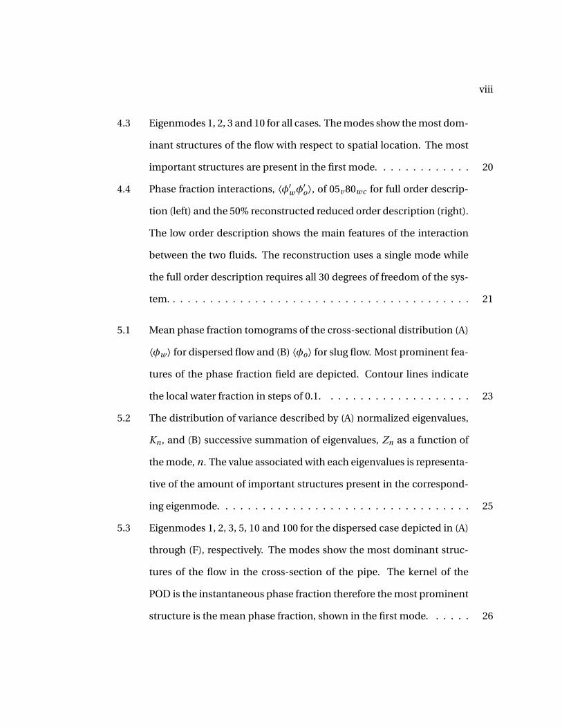
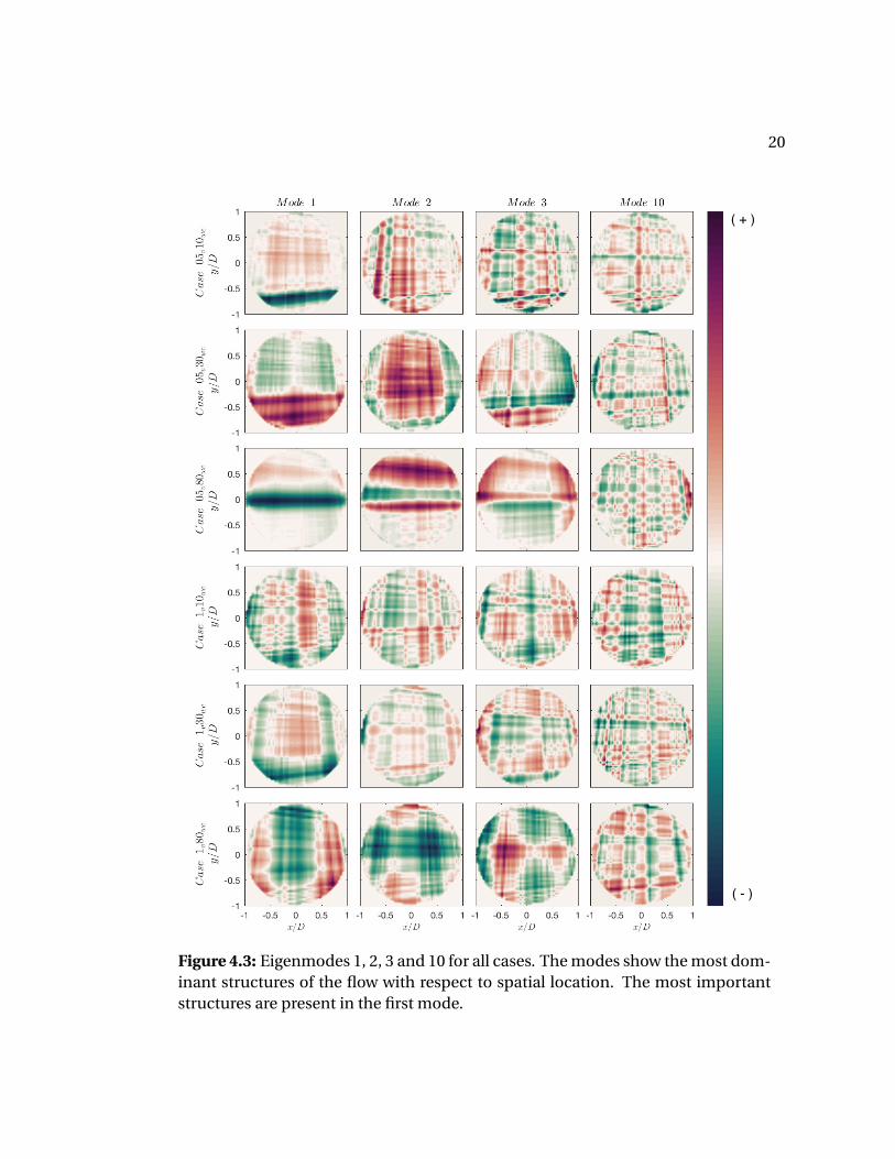
4.3 Eigenmodes 1, 2, 3 and 10 for all cases. The modes show the most dom-

inant structures of the flow with respect to spatial location. The most

important structures are present in the first mode. . . . . . . . . . . . . 20

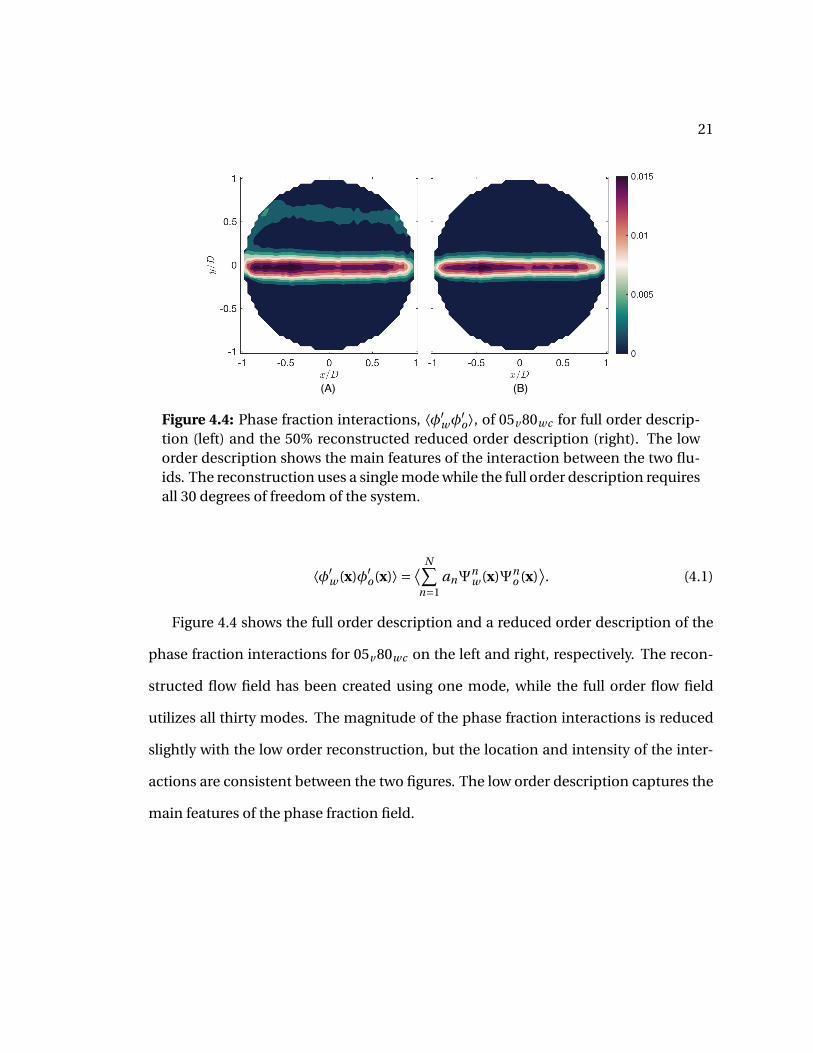
4.4 Phase fraction interactions, ⟨φ′wφ

′o⟩, of 05v 80wc for full order descrip-

tion (left) and the 50% reconstructed reduced order description (right).

The low order description shows the main features of the interaction

between the two fluids. The reconstruction uses a single mode while

the full order description requires all 30 degrees of freedom of the sys-

tem. . . . . . . . . . . . . . . . . . . . . . . . . . . . . . . . . . . . . . . . . 21

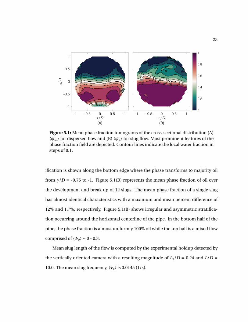
5.1 Mean phase fraction tomograms of the cross-sectional distribution (A)

⟨φw ⟩ for dispersed flow and (B) ⟨φo⟩ for slug flow. Most prominent fea-

tures of the phase fraction field are depicted. Contour lines indicate

the local water fraction in steps of 0.1. . . . . . . . . . . . . . . . . . . . 23

5.2 The distribution of variance described by (A) normalized eigenvalues,

Kn , and (B) successive summation of eigenvalues, Zn as a function of

the mode, n. The value associated with each eigenvalues is representa-

tive of the amount of important structures present in the correspond-

ing eigenmode. . . . . . . . . . . . . . . . . . . . . . . . . . . . . . . . . . 25

5.3 Eigenmodes 1, 2, 3, 5, 10 and 100 for the dispersed case depicted in (A)

through (F), respectively. The modes show the most dominant struc-

tures of the flow in the cross-section of the pipe. The kernel of the

POD is the instantaneous phase fraction therefore the most prominent

structure is the mean phase fraction, shown in the first mode. . . . . . 26

ix

5.4 Eigenmodes 1, 2, 3, 5, 10 and 100 for the slug flow case depicted in (A)

through (F), respectively. The first mode shows the mean phase frac-

tion of the slug flow with successive modes depicting the main features

of the flow spatially. . . . . . . . . . . . . . . . . . . . . . . . . . . . . . . 27

5.5 (A) Full order instantaneous phase fraction tomograms and (B) re-

duced order instantaneous phase fraction tomograms of dispersed

flow, reconstructed with 1 eigenmode. The low order description

shows main features of the flow while using less than 1% of the infor-

mation from the full order model. . . . . . . . . . . . . . . . . . . . . . . 29

5.6 (A) Full order instantaneous phase fraction tomograms and (B) re-

duced order instantaneous phase fraction tomograms of slug flow, re-

constructed with 3 eigenmodes. The reduced order dynamical descrip-

tion includes prominent flow features using three degrees of freedom.

The full order description of the flow uses 1250 degrees of freedom. . . 29

5.7 Phase correlation diagrams of temporal coefficients for i = 1, 2&3 for

dispersed flow (left column) and slug flow (right column). The aster-

isk and the square, included in the figures of slug flow, represent the

formation at t = to and break up at t = t f of the slug, respectively. . . . 31

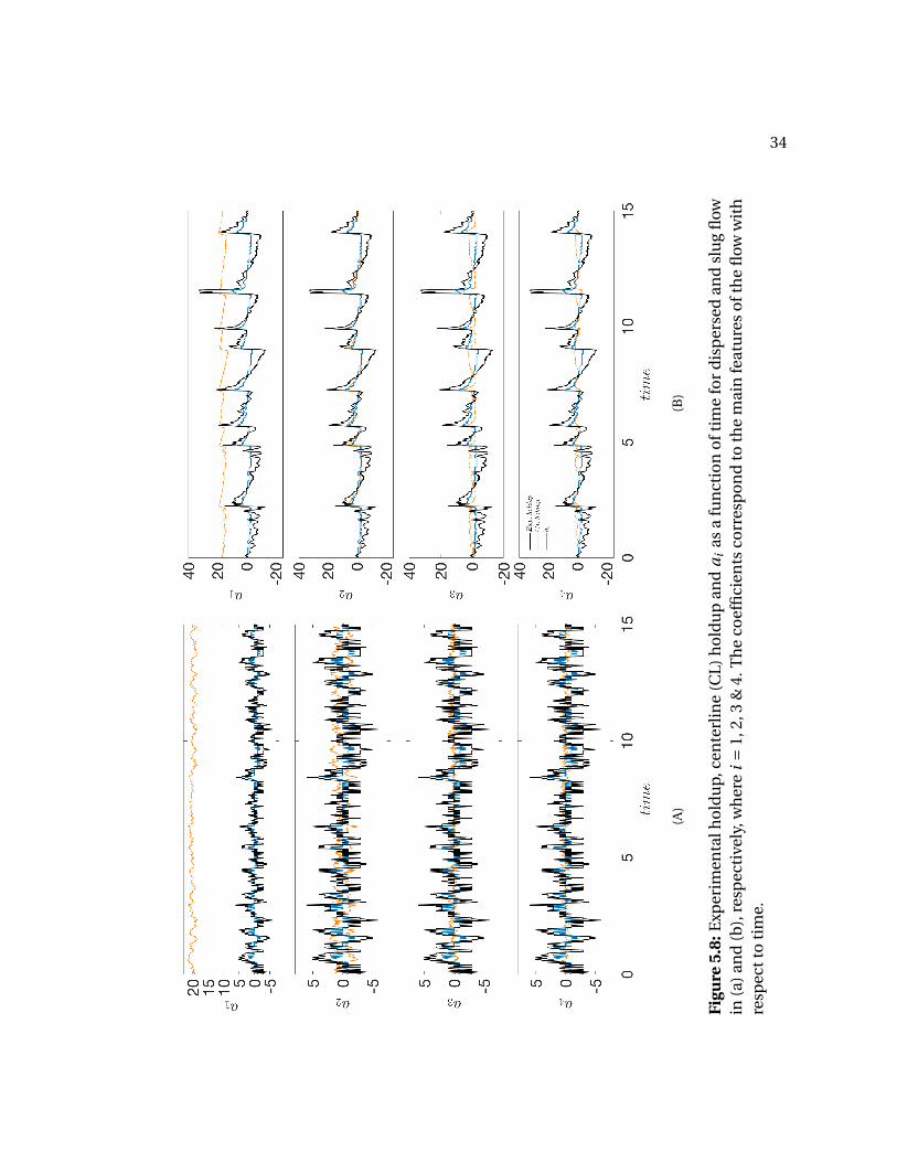
5.8 Experimental holdup, centerline (CL) holdup and ai as a function of

time for dispersed and slug flow in (a) and (b), respectively, where i =1, 2, 3 & 4. The coefficients correspond to the main features of the flow

with respect to time. . . . . . . . . . . . . . . . . . . . . . . . . . . . . . . 34

x

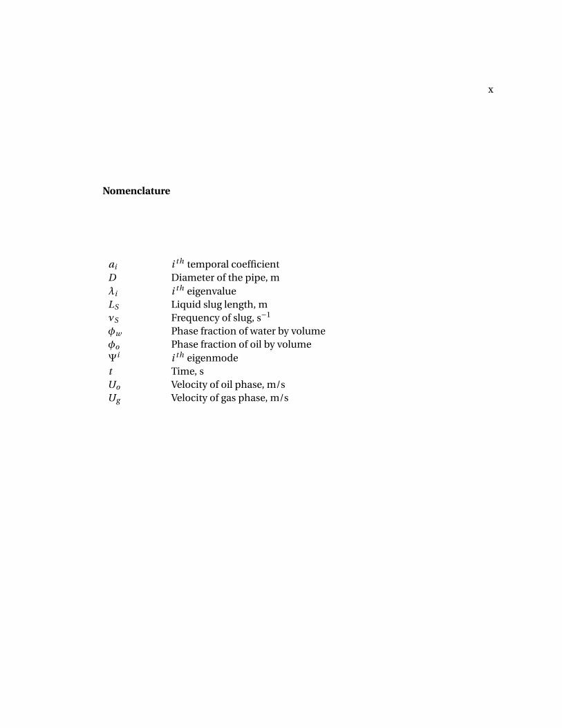
Nomenclature

ai i th temporal coefficientD Diameter of the pipe, mλi i th eigenvalueLS Liquid slug length, mνS Frequency of slug, s−1

φw Phase fraction of water by volumeφo Phase fraction of oil by volumeΨi i th eigenmodet Time, sUo Velocity of oil phase, m/sUg Velocity of gas phase, m/s

1

Chapter 1

Introduction and Motivation

Multiphase flows appear in a variety of industrial applications including; petroleum

production and transportation systems, production of polymers and other materials,

fluidized beds, boiler and heat exchangers tubes and hydroelectric power [3, 6, 9, 15,

19, 21]. Multiphase flow has complex characteristics such as differences in pressure

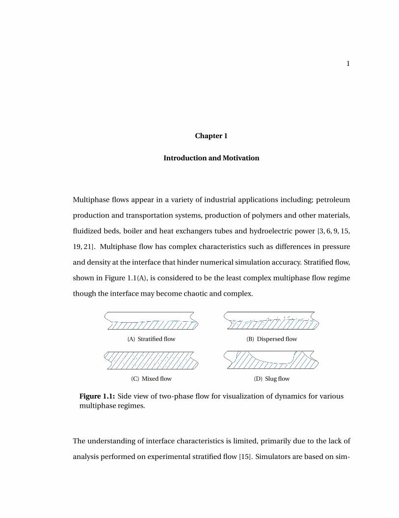
and density at the interface that hinder numerical simulation accuracy. Stratified flow,

shown in Figure 1.1(A), is considered to be the least complex multiphase flow regime

though the interface may become chaotic and complex.

(A) Stratified flow (B) Dispersed flow

(C) Mixed flow (D) Slug flow

Figure 1.1: Side view of two-phase flow for visualization of dynamics for variousmultiphase regimes.

The understanding of interface characteristics is limited, primarily due to the lack of

analysis performed on experimental stratified flow [15]. Simulators are based on sim-

2

plified models or assumptions concerning the interfacial and dispersion behavior of

the phenomena, both of which hinder accuracy of the predictions.

Dispersed flow, shown in Figure 1.1(B), is characterized by the distribution of one

fluid, the dispersed phase, within another fluid, the carrier phase. Although inter-

face development is considered of secondary importance to the particle size spectra

in most dispersed flow analysis, there is correlation between the geometric character-

istics of the interface and droplet break up and coalescence [3]. Dispersed flow is often

analyzed via numerical simulations but the complexity and scale of the dispersed fluid

deem these approaches either inaccurate at the macroscale level or challenging and

computationally expensive at the fully resolved level [3]. Mixed flow occurs when there

is not a well defined interface between the two fluids, as seen in Figure 1.1(C).

Phase inversion is a phenomenon where the dispersed phase and the carrier phase

spontaneously invert due to a small change in the operational conditions. Brauner

and Ulmann [4] formulated a model for phase inversion in two-phase pipe flows. The

model provides explanations of features of the phonemena in liquid-liquid pipe flows

and static mixers and compares favorably with available data on critical holdup for

phase inversion. Liu et al . [22] used laser-induced fluorescence to study flow struc-

tures in liquid-liquid flows at high dispersed phase fractions. An unstable range was

found in which oil-in-water and water-in-oil dispersions could co-exist. This unstable

range was different from the ambivalent range seen in agitated flow systems, despite

the similar appearance.

Slug flow is intermittent two- or three-phase flow and exists for a wide range of

flow rates. A two fluid representation of the flow field is depicted in Figure 1.1(D).

Slug flow originates from stratified two-phase flow where small perturbations create

3

interfacial waves to grow via Kelvin-Helmoltz instabilities. This causes one phase to

entirely occupy the cross-section of the pipe [27]. Other causes of slug flow include

accumulation of liquid at nonuniform terrain valleys [1] as well as wave coalescence at

high flow rates [28].

In past studies of slug flow, characterization of the flow was carried out via slug

length and frequency, gas and liquid holdups and velocity fluctuations. Liquid holdup

refers to the percent liquid at an area of interest in the flow. The parameters are an-

alyzed with the intent of tracking and predicting slug development. Understanding

the formation and break up of slugs is critical in mitigating the intermittent loading it

inflicts on pipeline infrastructure. Serious problems occur as a result of pipe wall dam-

ages, especially in hydrocarbon production and transportation lines, leading to severe

safety risks [20].

Numerical and experimental studies have been performed to improve and adapt

current slug length and shape distribution predictions within the flow field [6, 8, 27].

The two-fluid model, used frequently in numerical analysis, is formulated by consid-

ering the cross-sectional averaged governing equations of mass and momentum for

each phase. Issa and Kempf [17] took a mechanistic approach to the prediction of

slug development, based on the numerical solution of the one-dimensional transient

two-fluid model equations. This approach minimized the need for phenomenologi-

cal models. Given the simplicity of the model, the results of the computations for slug

characteristics and data obtained from literature have remarkable agreement.

A one-dimensional two-fluid model was also used in a study by Hanyang and Liejin

[12] to investigate a viscous Kelvin-Helmholtz criterion of interfacial wave instability.

This study utilized a more complex closure relation including dynamic pressure terms

4

in lieu of hydrostatic approximation. The criterion predicts the stability limit of the

flow well in horizontal and nearly horizontal pipes. Predicted and experimental re-

sults also show that critical liquid height is insensitive to small pipe inclinations, but at

low gas velocities, critical liquid velocity and wave velocity are sensitive to small pipe

inclinations.

Carneiro et al . [6] examined slug flow numerically and experimentally. The slug

flow was simulated with a two-fluid model and verified via experimental measure-

ments. The two-fluid model was used to predict frequency, velocity and slug length

which showed good agreement to the experimental measurements with differences

varying from 10% to 20% for frequency and slug length. Hu et al . [15] used a fast-

response X-ray tomography system to analyze the flow structure and phase distribu-

tion in two- and three-phase experimental stratified and slug flows. The experimental

results suggested that the commonly used one-dimensional two-fluid model should

not only account for cross-sectional distribution of phase fraction and velocity, but

also their axial variation.

Hydroelectric power technology, an industrial application of multiphase flow, has

proved to be a highly flexible and controllable means of power production. Though

the technology is mature, there exists several fundamental fluid flow problems which

prevent running of a more cost effective plant. The widely used Francis turbine ex-

periences significant drops in efficiency when operating in off-design conditions [13].

Escalera et al . [10] experimentally investigated hydraulic turbines to evaluate the de-

tection of cavitation. It was found that the bubble growth could be approximated by

the generalized Rayleigh-Plesset equation. The use of this equation requires that the

bubble pressure and infinite domain pressure are known. Bajic [2] analytically for-

5

mulated a novel technique for vibro-acoustical diagnostics of turbine cavitation and

demonstrated its use on a Francis turbine. Diagnostic results formed the basis for

setting up a high-sensitivity cavitation monitoring system. Predictive maintenance

management systems have been studied by Fu et al . [11], with the introduction of a

intelligent-control-maintenance-management system platform. Tests are run on an

artificial model with results showing that the proposed strategy can guarantee ideal

performance.

Proper orthogonal decomposition (POD) can be used to characterize the complex

multiphase flow mechanics to understand the dynamical field. Cizmas et al . [7] stud-

ied the interactions of gas and solid phases in fluidized beds to explore the implemen-

tation of a reduced order model via Galerkin methods. The data were obtained using

the Multiphase Flow with Interface eXchange code to simulate the two-dimensional

fluidization flow field. Cizmas et al . found that the most dominant characteristics of

motion can be captured by a small number of POD modes. As expected, in order to

capture the fine details of the spatial features of the flow, a large number of modes are

needed. Phase correlation diagrams revealed the existence of a low-dimensional at-

tractor due to the closed circular behavior of the coefficients a2 and a3 with respect to

a1.

Brenner et al . [5] studied isothermal and non-isothermal multiphase flow in flu-

idized beds. Brenner et al . present the derivation and implementation of a reduced-

order model (ROM) based on proper orthogonal decomposition. Two methods are

utilized for clustering snapshots in the transient region, a coupled and split approach.

The split method required an autocorrelation matrix to be computed for each vari-

able. In the coupled method, prior to computation the variables are concatenated.

6

The study found the split approach to yield less error for the given case.

The POD examples discussed in the previous paragraph use simulation data to con-

struct the kernel of POD formulation and subsequent analysis. This study implements

proper orthogonal decomposition on measurement data from stratified, mixed, dis-

persed and slug flow in a large diameter pipe. By using experimental multiphase flow

data, the mathematical representation pertains to parameters of the flow field. More

specifically, all characteristics observed through this analysis are directly related to the

flow dynamics, no assumptions are hindering the accuracy of the resulting mathemat-

ical descriptions.

Four flow regimes are investigated. For stratified and mixed flow, cases with a water

content percentage of 10%, 30% and 80% are considered, six cases in total. These cases

are analyzed to identify the features of the flow that vary as a function of the velocity of

the fluid as well as the water-to-oil ratio in the pipe. Dispersed and slug flow are then

investigated to gain insight into dynamics of more complex flow fields. These regimes

are also prevalent in industrial applications. The characterization of these regimes can

lead to increased efficiency of transportation systems of petroleum, tube and shell heat

exchangers and polymer production systems to name a few. In particular, the identi-

fication of slug initiation and evolution can be used mitigate the irregular loading on

pipe infrastructure.

7

Chapter 2

Theory

2.1 Slug parameters

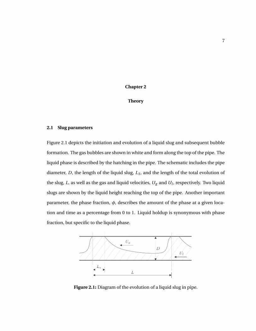
Figure 2.1 depicts the initiation and evolution of a liquid slug and subsequent bubble

formation. The gas bubbles are shown in white and form along the top of the pipe. The

liquid phase is described by the hatching in the pipe. The schematic includes the pipe

diameter, D , the length of the liquid slug, LS , and the length of the total evolution of

the slug, L, as well as the gas and liquid velocities, Ug and Ul , respectively. Two liquid

slugs are shown by the liquid height reaching the top of the pipe. Another important

parameter, the phase fraction, φ, describes the amount of the phase at a given loca-

tion and time as a percentage from 0 to 1. Liquid holdup is synonymous with phase

fraction, but specific to the liquid phase.

Figure 2.1: Diagram of the evolution of a liquid slug in pipe.

8

Given the velocity of the liquid phase, and considering it to be constant throughout

the pipe, the length of slug k is

LS,k =Ul∆ta→b , (2.1)

where Ul is the liquid velocity and time, t , is taken from the head, a, to the tail, b, of

the slug [6].

The slug frequency is determined by the number of slugs that pass through an area

of interest during a controlled time interval. The average slug frequency is defined as

⟨νs⟩ = 1

Nk

Nk∑k=1

1

∆tk, (2.2)

where the frequency is averaged over the total number of slugs, Nk .

2.2 Proper orthogonal decomposition

Proper orthogonal decomposition produces an organized basis of modes and eigenval-

ues representing the amount of variance corresponding to each mode. The structures

of the flow are organized based on the kernel of the decomposition. Classical POD was

introduced to fluid mechanics to analyze turbulent velocity signals [23]. The method

of snapshots was modified by Sirovich [26] and applied when the flow measurements

contain high spatial resolution in comparison to temporal resolution (cf. Holmes [14]).

For snapshot POD, a spatial correlation matrix is used to compute eigenfunctions,

decorrelating structures contained in the snapshots. The two-point spatial correlation

tensor is defined as

9

R(x,x′) = 1

N

N∑n=1

φ(x, t n)φT (x′, t n), (2.3)

where φ(x, t n) is the phase fraction field, t n is the time at a sample n, N refers to the

number of snapshots, bold symbols represent vector arrays and the prime represents

the spatial coordinate of another point in the domain. R(x,x′) becomes the kernel of

the POD. The kernel varies amongst the cases. For the stratified and mixed flow anal-

ysis, the kernel is the fluctuating phase fraction. For dispersed and slug flow analysis,

the kernel is the instantaneous phase fraction. Assuming the basis modes can be writ-

ten in terms of the original data and a coefficient A, then the basis modes,

Ψi (x) =N∑

i=1A(t i )φ(x, t i ) (2.4)

has the largest projection on the phase fraction field in a mean square sense. The so-

lution of the POD integral equation,

ˆΩ

R(x,x′)Ψi (x′)dx′ =λiΨi (x) (2.5)

yields a complete set of orthogonal eigenfunctions. The substitution of Equations 2.3

and 2.4 into the POD integral equation and the discretization results in an eigenvalue

problem described as

CA =λA, (2.6)

where the coefficient vector, A = [A(t 1), A(t 2), ..., A(t n)

]T , C is a symmetric N×N matrix

with components C j k = 1/N(φT (x, t j )φ(x, t k )

)and j ,k = 1, ..., N . λ is a diagonal matrix

10

of N eigenvalues where the eigenvalues and associated eigenmodes are ordered by

their proportion of variance, λ1 >λ2 >λ3 > ·· · >λn .

According to the eigenvalue problem, the set of coefficients are obtained from the

solution of Equation 2.6. The modes are normalized and formed into an orthonormal

basis that is defined as

Ψi (x) =∑N

i=1 Ai (t n)φ(x, t n)

||∑Ni=1 Ai (t n)φ(x, t n)|| . (2.7)

Using the eigenfunctions of the POD, the phase fraction tomograms may be recon-

structed as

φ(x, t n) =N∑

i=1aiΨ

i (x), (2.8)

where the set of coefficients, ai , are obtained by back-projecting the phase fraction

tomograms onto the deterministic POD modes. In the domain Ω, the coefficients are

defined as

ai =ˆΩ

φ(x, t n)Ψi (x)dx′. (2.9)

and represent the most prominent features of the flow as a function of time.

A set of eigenfunctions that represent the modes of turbulence and eigenvalues that

measure the variance associated with each eigenfunction are provided from the POD

analysis. The self-normalized eigenvalues,

Kn =λn/N∑

i=1λi , (2.10)

11

describes the percent of information associated with a given eigenmode n. The sum of

the eigenvalues shows the distribution of variance, therefore the variance contained in

the first n eigenmodes is equal to

Zn =∑n

k=1λk∑Ni=1λi

, n = 1,2, . . . , N . (2.11)

12

Chapter 3

Experimental Setup

3.1 Well Flow Loop

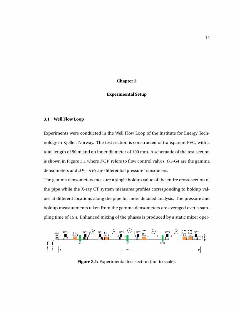
Experiments were conducted in the Well Flow Loop of the Institute for Energy Tech-

nology in Kjeller, Norway. The test section is constructed of transparent PVC, with a

total length of 50 m and an inner diameter of 100 mm. A schematic of the test section

is shown in Figure 3.1 where FCV refers to flow control valves, G1-G4 are the gamma

densometers and dP1- dP7 are differential pressure transducers.

The gamma densometers measure a single holdup value of the entire cross-section of

the pipe while the X-ray CT system measures profiles corresponding to holdup val-

ues at different locations along the pipe for more detailed analysis. The pressure and

holdup measurements taken from the gamma densometers are averaged over a sam-

pling time of 15 s. Enhanced mixing of the phases is produced by a static mixer oper-

Figure 3.1: Experimental test section (not to scale).

13

Figure 3.2: Orientation of source and detection devices for one X-ray system alongthe pipe.

ating directly after the injection site of the two fluids into the pipe. The test section is

horizontally aligned at 0±0.1.

3.2 X-ray computed tomography system

The X-ray tomography system is comprised of up to six point sources and six detectors.

The system consists of two triangular setups, each containing three cameras and three

sources at adjustable position along the pipe shown by X-ray cameras 1-3 and 4-6 in

Figure 3.1. For reference, one triangular setup is shown in Figure 3.2.

Each X-ray is attenuated as it passes through the air, the pipe wall and the fluids

inside the pipe, with stronger attenuation indicated by lower intensity of the camera

pixel. Calibration images are obtained by filling the pipe entirely with gas, oil or water.

This allows for the pixel value to be converted to a phase content percentage value,

referred to as holdup value, for the calibrated phases. Two-dimensional tomograms

may be constructed from the profiles of holdup measured by X-ray detectors shown

in Figure 3.2. The dimension of a single pixel is 0.1 mm x 0.1 mm. For noise reduc-

tion, groups of neighboring pixels are averaged and the final resolution is therefore 2

14

Table 3.1: Experimental test conditions.

Flow regime Case Phase-Phase Umi x (m/s) X-ray system Total snapshots

Stratified 05v 10wc oil-water 0.5 2 sources 30Stratified 05v 30wc oil-water 0.5 2 sources 30Stratified 05v 80wc oil-water 0.5 2 sources 30Mixed 1v 10wc oil-water 1 2 sources 100Mixed 1v 30wc oil-water 1 2 sources 100Mixed 1v 80wc oil-water 1 2 sources 100Dispersed - oil-water 1 6 sources 1232Slug - gas-oil 1.5 6 sources 1250

mm/pixel.

Table 3.1 shows details of the test parameters. Eight experiments of two-phase flow

are analyzed to compare characteristics of the four considered regimes. The stratified

and mixed flow cases utilize water and oil as the two-phases. Three cases of both strat-

ified and mixed flow with varying water content of 10%, 30% and 80% are investigated

to better understand dynamics of the flow fields. The velocity and water content val-

ues are signified by the subscripts v and wc of the case for future annotation (Table 3.1).

Finally, the dispersed flow and slug flow are analyzed separately. The dispersed flow,

comprised of oil and water, and slug flow, comprised of gas and oil, utilize X-ray detec-

tors 1-3 and 4-6 for a more detailed construction of the tomogram. Dispersed and slug

flow also contain an increased number of snapshots for more detailed analysis. The

sum of the velocities of the two phases is the mixed velocity, Umi x , obtained from the

inlet pump velocity of each fluid.

15

Chapter 4

Results: Stratified and Mixed Flow

The stratified and mixed flow cases are examined to describe the dynamics of the flow

as a function of water content and velocity. The multiple cases considered for each

flow regime allow for in-depth analysis of the dominant characteristics, such as inter-

actions between the two fluids, stratification layer geometries and droplet dispersion

and accumulation. Trends found via POD will give insight into the dynamical features

and phase interactions as a function of the velocity and water content.

4.1 Time-averaged statistics

Tomograms of the mean phase fraction of water, ⟨φw ⟩, for all six cases are shown in Fig-

ure 4.1. The spatial coordinates are normalized by the pipe diameter, D and ⟨·⟩ denotes

ensemble averaging. The three lower velocity cases, in the upper half of Figure 4.1, are

in the stratified flow regime, with coherent layers of percent water in the vertical di-

rection. For the W C = 10% case, the majority of the pipe has uniform phase fraction

of pure oil for the upper 7/8 of the pipe. As the water content increases for the low

velocity cases, the layers become thicker and more pronounced. For the W C = 30%

case, the stratification initiates near the center of the pipe, continuing to the bottom.

The highest water content case shows stratified layers starting near the top of the pipe,

16

Figure 4.1: Time-averaged tomograms of the cross-sectional water distributionfor stratified and mixed flow cases. The time-averaged tomograms show the mostprominent characteristics of the flow field. Contour lines indicate the local waterfraction in steps of 0.1.

with ∼100% water phase fraction reached by the center of the pipe. The 1 m/s velocity

cases indicate a highly mixed flow with the mean phase fraction showing less unifor-

mity as the water fraction changes. Water droplets are more uniformly distributed over

the cross-section for the low water content case, W C = 10%. As the water content in-

creases, the dispersed oil starts to increase toward the top of the pipe. For the W C =30% and W C = 80% cases, layers form in the vertical direction, but the majority of the

flow does not reach uniform oil or water phase inside the pipe.

17

4.2 Proper orthogonal decomposition

Figure 4.2 shows the distribution of the important variant structures associated with

phase fraction fluctuations as a function of the eigenvalue. In Figure 4.2(A), the

amount of variance for a given eigenvalue is shown, where Kn is obtained via Equa-

tion 2.10. For all six cases the first mode contains the largest portion of variance, with

percentages ranging from 5.5% to 64.4%. The three low velocity cases exhibit a sub-

stantial decrease of pertinent information from mode 1 to mode 2. The highest water

content case, 05v 80wc , contains the most information in the first mode. As water con-

tent decreases, the value of the first mode also decreases. The large reduction of Kn

from mode to mode is not seen in the cases with high velocity. This is attributed to the

higher level of mixing occurring in the 1 m/s velocity cases compared to the stratified

flow depicted by the 0.5 m/s velocity cases.

The percentage of contribution of the successive eigenvalues is depicted in Figure

4.2(B). The sum of the eigenvalues is equivalent to the information provided by the

associated with phase fluctuations, therefore the amount of information contained in

the first n eigenvalues is defined by Equation 2.11. In Figure 4.2(B), the three high ve-

locity cases show similar convergence characteristics to each other when compared to

the three low velocity cases. This is again due to the amount of mixing occurring when

the pipe is running at 1 m/s. The percent water content also affects the distribution

of important structures. At high water content the eigenvalues converge more rapidly

though the difference in converges is much less at v = 1 m/s than at v = 0.5 m/s.

Table 4.1 details the corresponding eigenmodes required for reconstructions of the

features for 50%, 75% and 95% of the phase fraction field. The convergence shown

in Figure 4.2 is quantified in the table, with trends verified. As is also shown in Fig-

18

100

101

102

n, modes

0

0.2

0.4

0.6

0.8

1

Kn

(A)

0 20 40 60 80 100

n, modes

0

0.2

0.4

0.6

0.8

1

Zn

05v10wc

05v30wc

05v80wc

1v10wc

1v30wc

1v80wc

(B)

Figure 4.2: The distribution of variance described by (A) normalized eigenvalues,Kn , and (B) successive summation of eigenvalues, Zn as a function of the mode,n. The value associated with each eigenvalues is representative of the amount ofinformation present in the corresponding eigenmode.

Table 4.1: Corresponding eigenmodes required for 50%, 75% and 95% reconstruc-tion for the stratified and mixed flow cases.

Case 50% 75% 95% Total snapshots

05v 10wc 5 12 23 3005v 30wc 3 8 21 3005v 80wc 1 2 12 301v 10wc 15 29 55 1001v 30wc 14 29 55 1001v 80wc 12 26 53 100

ure 4.2, the 0.5 m/s velocity cases converge more quickly than the high velocity cases.

More specifically 50% reconstruction of the flow is obtained three to twelve fold faster.

The convergence is also dependent on water content with increases in water content

showing a decreases in modes needed for reconstruction. This trend is more apparent

in the slower velocity cases, the high level of mixing involved in the 1 m/s velocity cases

de-emphasizes the correlation.

19

POD modes 1, 2, 3 and 10 are shown for all cases in Figure 4.3. The location and

coherence of the modal structures are of interest therefore units of the scale are not

included. The first mode of the three lower velocity cases show structures that corre-

spond to the location of stratification of the flow as seen in Figure 4.1. For the higher

velocity cases, mode 1 does not contain well defined structures. This correlates to the

mean phase fraction fields of the mixed flows depicted in Figure 4.1. As the eigen-

modes increase, the features become incoherent. The coherence of the structures

present in the modes corresponds to the water content of the cases. The highest water

content cases, 05v 80wc and 1v 80wc show the highest organization when compared to

their respective velocity cases. The structures become less defined as the water content

decreases and the two cases with the lowest percent water display incoherence almost

immediately.

The convergence of the cases, seen in Figure 4.2 is directly related to the structures

present in the eigenmodes. The cases that contain more coherence of the structures,

converge quickly when compared with their respective velocity cases. The phase frac-

tion can be described by the eigenmodes more easily due to the larger amount of im-

portant structures present in the initial modes and therefore the case converges more

quickly. Furthermore, the higher velocity cases show minimal coherence for all eigen-

modes due to mixing. This is depicted in Figure 4.2(A) by the gradually decreasing

slope of the line for the successive modes.

Using the eigenfunctions of the POD, the phase fraction fluctuations may be recon-

structed, and as a result, the interaction between the two phases, ⟨φ′wφ

′o⟩ is described

as

20

Figure 4.3: Eigenmodes 1, 2, 3 and 10 for all cases. The modes show the most dom-inant structures of the flow with respect to spatial location. The most importantstructures are present in the first mode.

21

Figure 4.4: Phase fraction interactions, ⟨φ′wφ

′o⟩, of 05v 80wc for full order descrip-

tion (left) and the 50% reconstructed reduced order description (right). The loworder description shows the main features of the interaction between the two flu-ids. The reconstruction uses a single mode while the full order description requiresall 30 degrees of freedom of the system.

⟨φ′w (x)φ′

o(x)⟩ = ⟨ N∑n=1

anΨnw (x)Ψn

o (x)⟩

. (4.1)

Figure 4.4 shows the full order description and a reduced order description of the

phase fraction interactions for 05v 80wc on the left and right, respectively. The recon-

structed flow field has been created using one mode, while the full order flow field

utilizes all thirty modes. The magnitude of the phase fraction interactions is reduced

slightly with the low order reconstruction, but the location and intensity of the inter-

actions are consistent between the two figures. The low order description captures the

main features of the phase fraction field.

22

Chapter 5

Results: Dispersed and Slug Flow

Dispersed flow contains complex flow dynamics due to the droplets of each fluid being

enveloped in the other fluid, creating an ill-defined interface between the two-phases.

Slug flow, another complex flow regime, is seen when instabilities grow at the interface

between the two-fluids due to small perturbations in the flow. Slug flow may lead to

safety risks due to the intermittent loading on the pipe walls. Proper orthogonal de-

composition of dispersed and slug flow provides mathematical relationships that per-

tain to the flow dynamics of the respective regime. These relationships may be used to

lessen effects of the irregular loading by controlling the flow upstream through condi-

tion monitoring.

5.1 Time-averaged statistics

Time-averaged tomograms of the mean phase fraction, ⟨φw ⟩, for the water-oil dis-

persed flow case and ⟨φo⟩, for the gas-oil slug flow case are shown in Figure 5.1. The

spatial coordinates are normalized by the pipe diameter, D . The mean phase fraction

of water for the dispersed flow shows a stratified layer, with a thickness of 0.25D , lo-

cated near the horizontal centerline of the pipe. There exist two symmetric pockets of

⟨φw ⟩ ∼ 100% in the bottom half of the pipe along the outside edges. An area of strat-

23

Figure 5.1: Mean phase fraction tomograms of the cross-sectional distribution (A)⟨φw ⟩ for dispersed flow and (B) ⟨φo⟩ for slug flow. Most prominent features of thephase fraction field are depicted. Contour lines indicate the local water fraction insteps of 0.1.

ification is shown along the bottom edge where the phase transforms to majority oil

from y/D = -0.75 to -1. Figure 5.1(B) represents the mean phase fraction of oil over

the development and break up of 12 slugs. The mean phase fraction of a single slug

has almost identical characteristics with a maximum and mean percent difference of

12% and 1.7%, respectively. Figure 5.1(B) shows irregular and asymmetric stratifica-

tion occurring around the horizontal centerline of the pipe. In the bottom half of the

pipe, the phase fraction is almost uniformly 100% oil while the top half is a mixed flow

comprised of ⟨φo⟩ ∼ 0 - 0.3.

Mean slug length of the flow is computed by the experimental holdup detected by

the vertically oriented camera with a resulting magnitude of Ls/D = 0.24 and L/D =10.0. The mean slug frequency, ⟨νs⟩ is 0.0145 (1/s).

24

5.2 Proper orthogonal decomposition

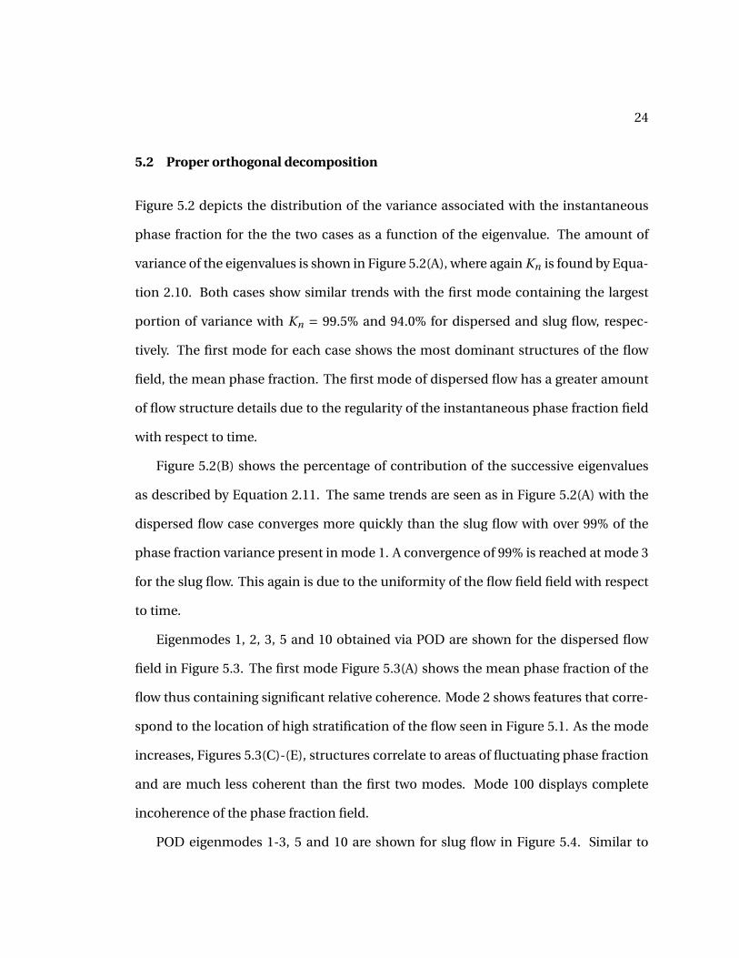
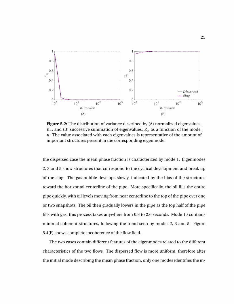
Figure 5.2 depicts the distribution of the variance associated with the instantaneous

phase fraction for the the two cases as a function of the eigenvalue. The amount of

variance of the eigenvalues is shown in Figure 5.2(A), where again Kn is found by Equa-

tion 2.10. Both cases show similar trends with the first mode containing the largest

portion of variance with Kn = 99.5% and 94.0% for dispersed and slug flow, respec-

tively. The first mode for each case shows the most dominant structures of the flow

field, the mean phase fraction. The first mode of dispersed flow has a greater amount

of flow structure details due to the regularity of the instantaneous phase fraction field

with respect to time.

Figure 5.2(B) shows the percentage of contribution of the successive eigenvalues

as described by Equation 2.11. The same trends are seen as in Figure 5.2(A) with the

dispersed flow case converges more quickly than the slug flow with over 99% of the

phase fraction variance present in mode 1. A convergence of 99% is reached at mode 3

for the slug flow. This again is due to the uniformity of the flow field field with respect

to time.

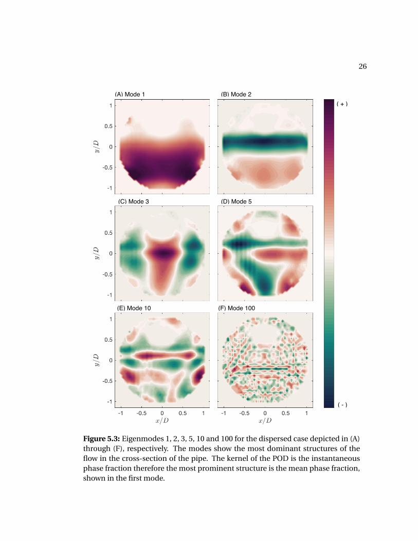
Eigenmodes 1, 2, 3, 5 and 10 obtained via POD are shown for the dispersed flow

field in Figure 5.3. The first mode Figure 5.3(A) shows the mean phase fraction of the

flow thus containing significant relative coherence. Mode 2 shows features that corre-

spond to the location of high stratification of the flow seen in Figure 5.1. As the mode

increases, Figures 5.3(C)-(E), structures correlate to areas of fluctuating phase fraction

and are much less coherent than the first two modes. Mode 100 displays complete

incoherence of the phase fraction field.

POD eigenmodes 1-3, 5 and 10 are shown for slug flow in Figure 5.4. Similar to

25

100

101

102

103

n, modes

0

0.2

0.4

0.6

0.8

1

Kn

(A)

100

101

102

103

n, modes

0

0.2

0.4

0.6

0.8

1

Zn

Dispersed

Slug

(B)

Figure 5.2: The distribution of variance described by (A) normalized eigenvalues,Kn , and (B) successive summation of eigenvalues, Zn as a function of the mode,n. The value associated with each eigenvalues is representative of the amount ofimportant structures present in the corresponding eigenmode.

the dispersed case the mean phase fraction is characterized by mode 1. Eigenmodes

2, 3 and 5 show structures that correspond to the cyclical development and break up

of the slug. The gas bubble develops slowly, indicated by the bias of the structures

toward the horizontal centerline of the pipe. More specifically, the oil fills the entire

pipe quickly, with oil levels moving from near centerline to the top of the pipe over one

or two snapshots. The oil then gradually lowers in the pipe as the top half of the pipe

fills with gas, this process takes anywhere from 0.8 to 2.6 seconds. Mode 10 contains

minimal coherent structures, following the trend seen by modes 2, 3 and 5. Figure

5.4(F) shows complete incoherence of the flow field.

The two cases contain different features of the eigenmodes related to the different

characteristics of the two flows. The dispersed flow is more uniform, therefore after

the initial mode describing the mean phase fraction, only one modes identifies the in-

26

Figure 5.3: Eigenmodes 1, 2, 3, 5, 10 and 100 for the dispersed case depicted in (A)through (F), respectively. The modes show the most dominant structures of theflow in the cross-section of the pipe. The kernel of the POD is the instantaneousphase fraction therefore the most prominent structure is the mean phase fraction,shown in the first mode.

27

Figure 5.4: Eigenmodes 1, 2, 3, 5, 10 and 100 for the slug flow case depicted in (A)through (F), respectively. The first mode shows the mean phase fraction of the slugflow with successive modes depicting the main features of the flow spatially.

28

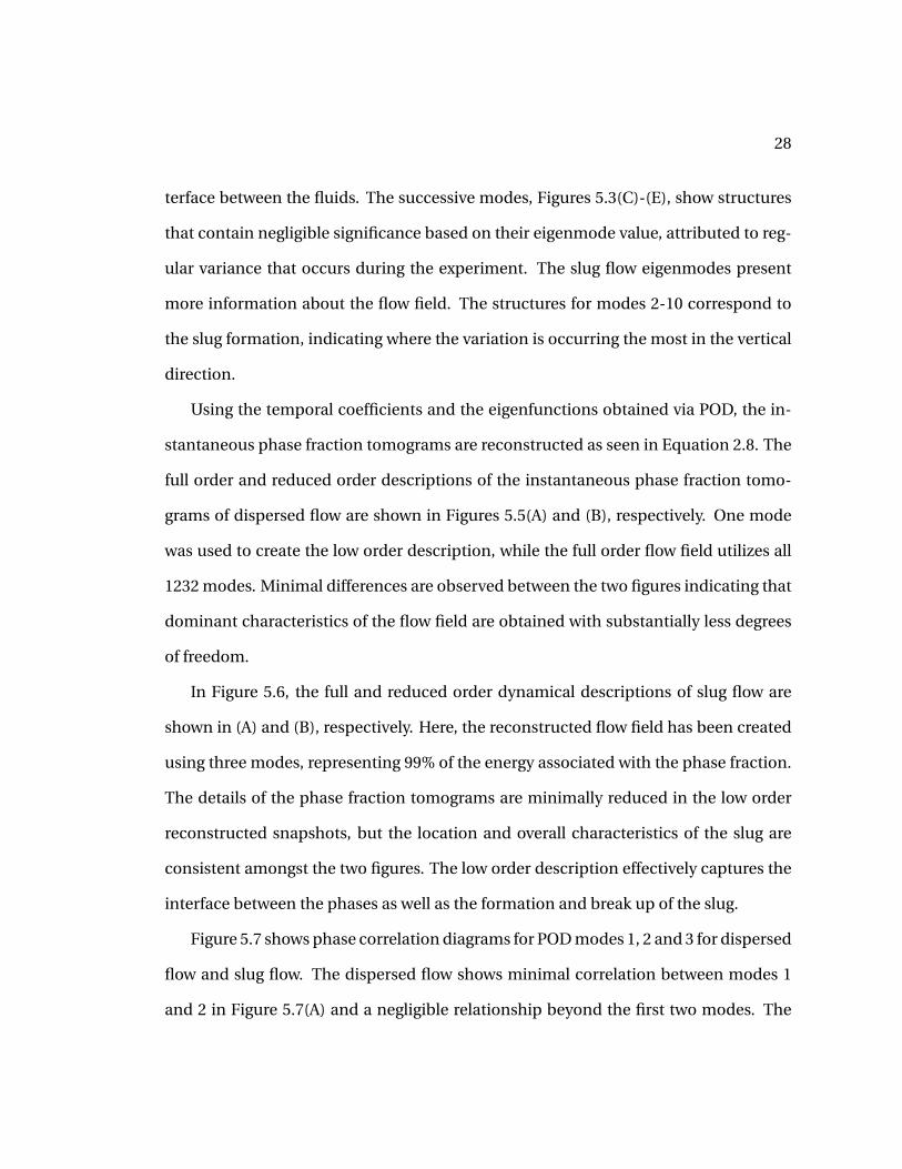
terface between the fluids. The successive modes, Figures 5.3(C)-(E), show structures

that contain negligible significance based on their eigenmode value, attributed to reg-

ular variance that occurs during the experiment. The slug flow eigenmodes present

more information about the flow field. The structures for modes 2-10 correspond to

the slug formation, indicating where the variation is occurring the most in the vertical

direction.

Using the temporal coefficients and the eigenfunctions obtained via POD, the in-

stantaneous phase fraction tomograms are reconstructed as seen in Equation 2.8. The

full order and reduced order descriptions of the instantaneous phase fraction tomo-

grams of dispersed flow are shown in Figures 5.5(A) and (B), respectively. One mode

was used to create the low order description, while the full order flow field utilizes all

1232 modes. Minimal differences are observed between the two figures indicating that

dominant characteristics of the flow field are obtained with substantially less degrees

of freedom.

In Figure 5.6, the full and reduced order dynamical descriptions of slug flow are

shown in (A) and (B), respectively. Here, the reconstructed flow field has been created

using three modes, representing 99% of the energy associated with the phase fraction.

The details of the phase fraction tomograms are minimally reduced in the low order

reconstructed snapshots, but the location and overall characteristics of the slug are

consistent amongst the two figures. The low order description effectively captures the

interface between the phases as well as the formation and break up of the slug.

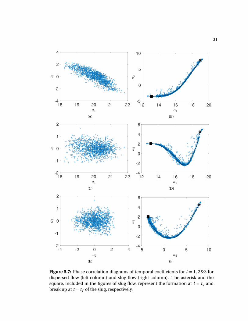
Figure 5.7 shows phase correlation diagrams for POD modes 1, 2 and 3 for dispersed

flow and slug flow. The dispersed flow shows minimal correlation between modes 1

and 2 in Figure 5.7(A) and a negligible relationship beyond the first two modes. The

29

(A) (B)

Figure 5.5: (A) Full order instantaneous phase fraction tomograms and (B) reducedorder instantaneous phase fraction tomograms of dispersed flow, reconstructedwith 1 eigenmode. The low order description shows main features of the flow whileusing less than 1% of the information from the full order model.

(A) (B)

Figure 5.6: (A) Full order instantaneous phase fraction tomograms and (B) reducedorder instantaneous phase fraction tomograms of slug flow, reconstructed with 3eigenmodes. The reduced order dynamical description includes prominent flowfeatures using three degrees of freedom. The full order description of the flow uses1250 degrees of freedom.

30

linear relationship seen between the modes 1 and 2 is inversely proportional signifying

that as a1 increases a2 decreases. The cyclical characteristics of the slug flow create

correlations between the first three modes as seen in Figures 5.7(B), 5.7(D) and 5.7(F).

The development of the slug spans the curves as specified in the figures denoted by

the asterisk, indicating the start of the slug and the square, signifying the end of the

slug. The relationship between a1 and a2 as well as a2 and a3 can be described by a

2nd order polynomial, 0.46x2−12.7x+84.8 and 0.17x2−0.45x−1.9, with R2= 0.99 and

0.93, respectively. The curve depicted by a1 and a3 is best described by a 3rd order

polynomial, 0.24x3 −10.9x2 +165.1x −827.1, with R2 = 0.92.

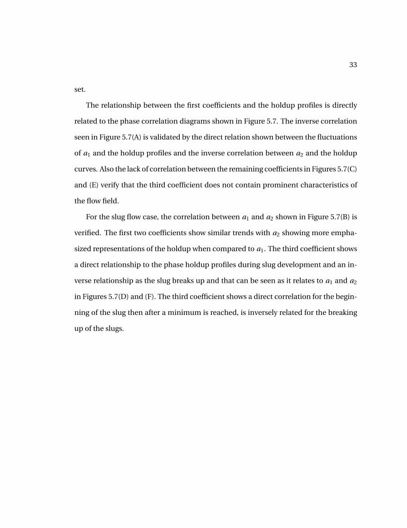
Figure 5.8 shows the two holdup profiles and coefficients ai as a function of time

where i = 1, 2, 3 and 4. The included profiles, experimental and centerline holdup, re-

fer to the holdup profile across the pipe detected by the vertically aligned camera and

the holdup profile taken as a function of the vertical array located at the center of the

pipe, respectively. t = 15-25 is omitted for clarity, the characteristics of the time steps

shown are indicative of the omitted data. In Figure 5.8(A), the experimental holdup

time series displays similar trends to the CL holdup, with fluctuations slightly empha-

sized. This discrepancy between the holdup profiles occurs due to the experimental

holdup measurement taking consideration the entirety of the domain. More specif-

ically, experimental holdup includes all x locations and centerline holdup considers

only one location at x/D = 0. The experimental holdup is commonly used in X-ray

CT data analysis [15, 25] to describe the liquid holdup as a function of vertical posi-

tion. This quantity directly relates to slug length based on the interface location as

a function of time, Equation 2.1. The first coefficient, although larger in magnitude,

shows the same trends displayed by the two holdup profiles, denoted as Exp. and CL.

31

18 19 20 21 22

a1

-4

-2

0

2

4a2

(A)

12 14 16 18 20

a1

-5

0

5

10

a2

(B)

18 19 20 21 22

a1

-2

-1

0

1

2

a3

(C)

12 14 16 18 20

a1

-4

-2

0

2

4

6

a3

(D)

-4 -2 0 2 4

a2

-2

-1

0

1

2

a3

(E)

-5 0 5 10

a2

-4

-2

0

2

4

6

a3

(F)

Figure 5.7: Phase correlation diagrams of temporal coefficients for i = 1, 2&3 fordispersed flow (left column) and slug flow (right column). The asterisk and thesquare, included in the figures of slug flow, represent the formation at t = to andbreak up at t = t f of the slug, respectively.

32

a2 shows an inverse relation to a1 as well as the experimental and CL holdup profiles.

As the temporal coefficient increases, a3, the trends are muted compared to the first

two coefficients, with a4 showing negligible fluctuations. The dispersed flow shows

fluctuations occurring within a small bandwidth. The variance of the holdup around

y/D = 0 is minimal when compared with mean phase fraction, depicted by a1. The

variance around y/D = 0 seen here is directly related to the energetic structure shown

in Figure 5.3(B).

The holdup profiles in Figure 5.8(B) exhibit cyclical fluctuations as the slug devel-

ops and breaks down. Similar to the dispersed case, the experimental holdup curve

shows an emphasized version of the CL holdup curve. The first coefficient displays

the same tendencies revealed by the holdup profiles but with dulled features. As the

coefficient increases, a2, the CL holdup is described well by the coefficient with the

mean percent difference between the two curves at 8.7%. As the coefficient increases,

i = 3, the coefficient shows a similar tendency to phase holdup during the first few

time instances surrounding the slug formation. Directly after the slug development,

a3 exhibits inverse fluctuations to those displayed by the two holdup profiles. By a4

the fluctuations of the curve are slightly muted with tendencies similar to the inverse

properties of the third coefficient.

The descriptions of the slug development by the second coefficient correlate to slug

length analysis as well. The mean slug length computed by the second temporal co-

efficient, Ls/D = 10.0, is the same magnitude as the mean slug length found from the

experimental holdup in Section 5.1. Similarly, the mean slug frequency for both meth-

ods of analysis ⟨νs⟩ = 0.0145 (1/s). The largest variation between the slug length found

from experimental holdup and from the POD temporal coefficients is 3.6% for this data

33

set.

The relationship between the first coefficients and the holdup profiles is directly

related to the phase correlation diagrams shown in Figure 5.7. The inverse correlation

seen in Figure 5.7(A) is validated by the direct relation shown between the fluctuations

of a1 and the holdup profiles and the inverse correlation between a2 and the holdup

curves. Also the lack of correlation between the remaining coefficients in Figures 5.7(C)

and (E) verify that the third coefficient does not contain prominent characteristics of

the flow field.

For the slug flow case, the correlation between a1 and a2 shown in Figure 5.7(B) is

verified. The first two coefficients show similar trends with a2 showing more empha-

sized representations of the holdup when compared to a1. The third coefficient shows

a direct relationship to the phase holdup profiles during slug development and an in-

verse relationship as the slug breaks up and that can be seen as it relates to a1 and a2

in Figures 5.7(D) and (F). The third coefficient shows a direct correlation for the begin-

ning of the slug then after a minimum is reached, is inversely related for the breaking

up of the slugs.

34

(A)

(B)

Figu

re5.

8:E

xper

imen

talh

old

up,

cen

terl

ine

(CL)

ho

ldu

pan

da

ias

afu

nct

ion

oft

ime

for

dis

per

sed

and

slu

gfl

owin

(a)

and

(b),

resp

ecti

vely

,wh

ere

i=

1,2,

3&

4.T

he

coef

fici

ents

corr

esp

on

dto

the

mai

nfe

atu

res

oft

he

flow

wit

hre

spec

tto

tim

e.

35

Chapter 6

Conclusion

Experiments were investigated to further understand phase fraction characteristics for

stratified, mixed, dispersed and slug flow. Proper orthogonal decomposition was per-

formed on all cases as well as statistical analysis on slug flow. For stratified flow, the

locations of coherent structures in the first few modes correspond to the locations of

the liquid-liquid interface. The same trend is not seen in the mixed flow cases, where

v = 1 m/s. The pronounced interface due to the high mixing of oil and water create

nearly incoherent structures in all modes. This observation is validated by the slow

convergence of the modes when compared to the low velocity cases. It was also ob-

served that for stratified flow, the main characteristics of the flow are described with a

small number of modes.

Mean slug length found via statistical analysis of experimental holdup and from

the second temporal coefficient were in perfect agreement. Over the sampling time

of 25 s, the dispersed flow is uniform with small fluctuations present at the liquid-

liquid interface. The liquid holdup of slug flow follows a periodic profile as a function

of time as slugs form and break up, with variation in frequency between the liquid

slugs. The dispersed case converges to 99% in the first mode, while slug flow reaches

99% convergence by mode 3. The eigenmodes show coherent features of the flow in

36

only the first few modes with mode 1 showing the mean phase fraction of the flow

for both cases. The interface of the fluids is depicted in mode 2 for dispersed flow

with little coherence seen in successive modes. The interface of the slug flow exists at

0 < y/D < 1 and is constantly in motion, which is seen by the layering of structures

in modes 2, 3, 5 and 10. Reconstructions, showing dominant features of the two flow

fields, are obtained with 1 and 3 modes for dispersed flow and slug flow, respectively.

Slug flow shows high dependence between temporal coefficients for i = 1, 2 and 3.

There exists a strong correlation between the dependent coefficients and the liquid

holdup. For dispersed flow this correlation is observed for modes 1 and 2. For slug

flow, this correlation is seen in the first four coefficients. The second coefficient, a2,

describes the centerline holdup of the slug flow with high accuracy.

The mathematical framework provided by POD via the eigenfunctions and tempo-

ral coefficients describe the dominant features with minimal degrees of freedom of the

systems. This translates to a large reduction of computational costs for further analysis

of the flow field. The descriptions provided can also be correlated to other flow param-

eters that are more easily implemented and less expensive than the X-ray CT system.

The relationship between the POD framework and the easily measured flow param-

eters can be used to develop flow control tools, improve multiphase simulations and

advance predictive methodologies in numerous industrial applications.

37

Chapter 7

Future Work

Building on the recognized relationships between holdup and temporal coefficients,

examination of correlations between flow characteristics obtained via POD and eas-

ily measurable flow parameters, for example instantaneous pressure fluctuations, will

be carried out. If relationships exist between the temporal coefficients and other pa-

rameters of the flow, then models can be constructed to identify variations in the flow

characteristics upstream from the location of interest as well as potential flow control

schemes to avoid such regimes. These systems can be implemented to improve con-

dition monitoring in many industrial applications.

Critical points will also be identified via the second derivative test by analyzing the

Hessian. Comparisons will be investigated between critical points and the tomograms

as well as the eigenmodes. The maxima, minima and saddle points obtained from

the second derivative test may be used to identify key locations in the cross-section of

the pipe, and further characterize the structures of the POD eigenmodes. The critical

points will also be compared with the dynamics of the flow shown by the temporal

coefficients. This comparison will relate the liquid holdup development with respect

to time and critical points at various spatial locations within the pipe. Poincaré maps

will also be produced to further study the dynamical system.

38

Finally, a low order dynamical system will be formulated for the flow fields. This

dynamical system will generate a set of parameters based on the POD temporal coef-

ficients to describe the flow. The system can then be descreetly calibrated based on

simpler flow parameters through transfer functions at specified time intervals to pro-

vide short and long term predictions of the flow dynamics.

39

Bibliography

[1] E. AL-SAFRAN, C. SARICA, H.-Q. ZHANG, AND J. BRILL, Investigation of slug flowcharacteristics in the valley of a hilly-terrain pipeline, International journal of mul-tiphase flow, 31 (2005), pp. 337–357.

[2] B. BAJIC, Multidimensional diagnostics of turbine cavitation, American Society ofMechanical Engineers Journal of Fluid Engineering, 124 (2002), pp. 943–950.

[3] S. BALACHANDAR AND J. K. EATON, Turbulent dispersed multiphase flow, AnnualReview of Fluid Mechanics, 42 (2010), pp. 111–133.

[4] N. BRAUNER AND A. ULLMANN, Modeling of phase inversion phenomenon in two-phase pipe flows, International Journal of Multiphase Flow, 28 (2002), pp. 1177–1204.

[5] T. A. BRENNER, R. L. FONTENOT, P. G. CIZMAS, T. J. O’BRIEN, AND R. W. BREAULT,A reduced-order model for heat transfer in multiphase flow and practical aspectsof the proper orthogonal decomposition, Computers & Chemical Engineering, 43(2012), pp. 68–80.

[6] J. N. E. CARNEIRO, R. FONSECA JR, A. J. ORTEGA, R. C. CHUCUYA, A. O. NIECK-ELE, AND L. F. A. AZEVEDO, Statistical characterization of two-phase slug flow in ahorizontal pipe, Journal of the Brazilian Society of Mechanical Sciences and Engi-neering, 33 (2011), pp. 251–258.

[7] P. G. CIZMAS, A. PALACIOS, T. O’BRIEN, AND M. SYAMLAL, Proper-orthogonal de-composition of spatio-temporal patterns in fluidized beds, Chemical engineeringscience, 58 (2003), pp. 4417–4427.

[8] M. COOK AND M. BEHNIA, Slug length prediction in near horizontal gas–liquidintermittent flow, Chemical Engineering Science, 55 (2000), pp. 2009–2018.

[9] M. P. DUDUKOVIC, F. LARACHI, AND P. L. MILLS, Multiphase reactors–revisited,Chemical Engineering Science, 54 (1999), pp. 1975–1995.

40

[10] X. ESCALER, E. EGUSQUIZA, M. FARHAT, F. AVELLAN, AND M. COUSSIRAT, Detec-tion of cavitation in hydraulic turbines, Mechanical systems and signal process-ing, 20 (2006), pp. 983–1007.

[11] C. FU, L. YE, Y. LIU, R. YU, B. IUNG, Y. CHENG, AND Y. ZENG, Predictive main-tenance in intelligent-control-maintenance-management system for hydroelectricgenerating unit, IEEE transactions on energy conversion, 19 (2004), pp. 179–186.

[12] G. U. HANYANG AND G. U. O. LIEJIN, Stability of stratified gas-liquid flow in hor-izontal and near horizontal pipes, Chinese Journal of Chemical Engineering, 15(2007), pp. 619–625.

[13] V. HASMATUCHI, M. FARHAT, S. ROTH, F. BOTERO, AND F. AVELLAN, Experimentalevidence of rotating stall in a pump-turbine at off-design conditions in generatingmode, Journal of Fluids Engineering, 133 (2011), p. 051104.

[14] P. HOLMES, J. L. LUMLEY, AND G. BERKOOZ, Turbulence, coherent structures, dy-namical systems and symmetry, Cambridge University Press, 1998.

[15] B. HU, M. LANGSHOLT, L. LIU, P. ANDERSSON, AND C. LAWRENCE, Flow structureand phase distribution in stratified and slug flows measured by x-ray tomography,International Journal of Multiphase Flow, 67 (2014), pp. 162–179.

[16] B. HU, C. STEWART, C. P. HALE, C. J. LAWRENCE, A. R. W. HALL, H. ZWIENS, AND

G. F. HEWITT, Development of an x-ray computed tomography (ct) system withsparse sources: application to three-phase pipe flow visualization, Experiments influids, 39 (2005), pp. 667–678.

[17] R. I. ISSA AND M. H. W. KEMPF, Simulation of slug flow in horizontal and nearlyhorizontal pipes with the two-fluid model, International journal of multiphaseflow, 29 (2003), pp. 69–95.

[18] U. KERTZSCHER, A. SEEGER, K. AFFELD, L. GOUBERGRITS, AND E. WELLNHOFER,X-ray based particle tracking velocimetry–a measurement technique for multi-phase flows and flows without optical access, Flow Measurement and Instrumen-tation, 15 (2004), pp. 199–206.

[19] P. KUMAR AND R. P. SAINI, Study of cavitation in hydro turbines - A review, Renew-able and Sustainable Energy Reviews, 14 (2010), pp. 374–383.

[20] O. KVERNVOLD, V. VINDØY, T. SØNTVEDT, A. SAASEN, AND S. SELMER-OLSEN,Velocity distribution in horizontal slug flow, International journal of multiphaseflow, 10 (1984), pp. 441–457.

41

[21] R. LINDKEN AND W. MERZKIRCH, A novel piv technique for measurements in mul-tiphase flows and its application to two-phase bubbly flows, Experiments in fluids,33 (2002), pp. 814–825.

[22] L. LIU, O. K. MATAR, C. J. LAWRENCE, AND G. F. HEWITT, Laser-induced fluores-cence (lif) studies of liquid–liquid flows. part i: flow structures and phase inversion,Chemical engineering science, 61 (2006), pp. 4007–4021.

[23] J. L. LUMLEY, The structure of inhomogeneous turbulent flows, Atmospheric tur-bulence and radio wave propagation, (1967), pp. 166–178.

[24] H. SCHÜMANN, M. TUTKUN, AND O. J. NYDAL, Experimental study of dispersedoil-water flow in a horizontal pipe with enhanced inlet mixing, Part 2: In-situdroplet measurements, Journal of Petroleum Science and Engineering, 145 (2016),pp. 753–762.

[25] H. SCHÜMANN, M. TUTKUN, Z. YANG, AND O. J. NYDAL, Experimental study ofdispersed oil-water flow in a horizontal pipe with enhanced inlet mixing, part 1:Flow patterns, phase distributions and pressure gradients, Journal of PetroleumScience and Engineering, 145 (2016), pp. 742–752.

[26] L. SIROVICH, Turbulence and the dynamics of coherent structures. Part I: Coherentstructures, Quarterly of applied mathematics, 45 (1987), pp. 561–571.

[27] Y. TAITEL AND A. E. DUKLER, A model for predicting flow regime transitions inhorizontal and near horizontal gas-liquid flow, AIChE Journal, 22 (1976), pp. 47–55.

[28] B. D. WOODS, Z. FAN, AND T. J. HANRATTY, Frequency and development of slugs ina horizontal pipe at large liquid flows, International Journal of Multiphase Flow,32 (2006), pp. 902–925.

[29] I. ZADRAZIL, O. K. MATAR, AND C. N. MARKIDES, An experimental characteriza-tion of downwards gas–liquid annular flow by laser-induced fluorescence: Flowregimes and film statistics, International Journal of Multiphase Flow, 60 (2014),pp. 87–102.