redalyc.on a finite moment perturbation of linear functionals and

Revista Integración

ISSN: 0120-419X

[email protected]

Universidad Industrial de Santander

Colombia

Fuentes, Edinson; Garza, Luis E.

On a finite moment perturbation of linear functionals and the inverse Szegó transformation

Revista Integración, vol. 34, núm. 1, 2016, pp. 39-58


Bucaramanga, Colombia

Available in: http://www.redalyc.org/articulo.oa?id=327045611003

How to cite

Complete issue

More information about this article

Journal's homepage in redalyc.org

Scientific Information System

Network of Scientific Journals from Latin America, the Caribbean, Spain and Portugal

Non-profit academic project, developed under the open access initiative

http://www.redalyc.org/revista.oa?id=3270


http://www.redalyc.org/articulo.oa?id=327045611003

http://www.redalyc.org/comocitar.oa?id=327045611003

http://www.redalyc.org/fasciculo.oa?id=3270&numero=45611

http://www.redalyc.org/articulo.oa?id=327045611003


http://www.redalyc.org

∮Revista Integración

Escuela de Matemáticas


Vol. 34, No. 1, 2016, pág. 39–58

On a finite moment perturbation of linear

functionals and the inverse Szegó

transformation

Edinson Fuentes a∗, Luis E. Garza b

a Universidad Pedagógica y Tecnológica de Colombia, Escuela de Matemáticas yEstadística, Tunja, Colombia.

b Universidad de Colima, Facultad de Ciencias, Colima, México.

Abstract. Given a sequence of moments cnn∈Z associated with an Hermi-tian linear functional L defined in the space of Laurent polynomials, we studya new functional LΩ which is a perturbation of L in such a way that a finitenumber of moments are perturbed. Necessary and sufficient conditions aregiven for the regularity of LΩ, and a connection formula between the corres-ponding families of orthogonal polynomials is obtained. On the other hand,assuming LΩ is positive definite, the perturbation is analyzed through theinverse Szegó transformation.Keywords: Orthogonal polynomials on the unit circle, perturbation of mo-ments, inverse Szegó transformation.MSC2010: 42C05, 33C45, 33D45, 33C47.

Sobre una perturbación finita de momentos de un

funcional lineal y la transformación inversa de Szegó

Resumen. Dada una sucesión de momentos cnn∈Z asociada a un funcionallineal hermitiano L definido en el espacio de los polinomios de Laurent, es-tudiamos un nuevo funcional LΩ que consiste en una perturbación de L detal forma que se perturba un número finito de momentos de la sucesión. Seencuentran condiciones necesarias y suficientes para la regularidad de LΩ, yse obtiene una fórmula de conexión que relaciona las familias de polinomiosortogonales correspondientes. Por otro lado, suponiendo que LΩ es definidopositivo, se analiza la perturbación mediante de la transformación inversa deSzegó.Palabras clave: Polinomios ortogonales en la circunferencia unidad, pertur-bación de momentos, transformación de Szegó inversa.

0∗E-mail: [email protected]: 13 October 2015, Accepted: 03 February 2016.To cite this article: E. Fuentes, L.E. Garza, On a finite moment perturbation of linear functionals and theinverse Szego transformation, Rev. Integr. Temas Mat. 34 (2016), No. 1, 39–58.

39

DOI: http://dx.doi.org/10.18273/revint.v34n1-2016003

40 E. Fuentes & L.E. Garza

1. Preliminaries and introduction

Consider a linear functional L defined in the linear space of Laurent polynomials Λ =spanznn∈Z such that L is Hermitian, i.e.,

cn = L, zn = L, z−n = c−n, n ∈ Z.

Then, a bilinear functional can be defined in the linear space P = spanznn≥0 ofpolynomials with complex coefficients by

p(z), q(z)L = L, p(z)q(z−1), p, q ∈ P.

The sequence of complex numbers cnn∈Z is called the sequence of moments associatedwith L. On the other hand, the Gram matrix associated with the canonical basis znn≥0

of P is

T =

c0 c1 · · · cn · · ·c−1 c0 · · · cn−1 · · ·...

.... . .

...c−n c−n+1 · · · c0 · · ·

......

.... . .

, (1)

which is known in the literature as Toeplitz matrix [7]. A sequence of monic polynomialsφnn≥0, with deg (φn) = n, is said to be orthogonal with respect to L if the condition

φn, φmL = δm,nkn,

where kn = 0, holds for every n,m 0. Notice that the sequence φnn≥0 can beobtained by using the Gram-Schmidt orthogonalization process with respect to the basisznn0. The necessary and sufficient conditions for the existence of such a sequencecan be expressed in terms of the Toeplitz matrix T: φnn≥0 satisfies the orthogonalitycondition if and only if Tn, the (n + 1) × (n + 1) principal leading submatrix of T, isnon-singular for every n ≥ 0. In such a case, L is said to be quasi-definite (or regular).On the other hand, if detTn > 0 for every n ≥ 0, then L is said to be positive definiteand it has the integral representation

L, p(z) =

T

p(z)dσ(z), p ∈ P, (2)

where σ is a nontrivial positive Borel measure supported on the unit circle T = z :|z| = 1. In such a case, there exists a (unique) family of polynomials ϕnn≥0, withdeg ϕn = n and positive leading coefficient, such that

T

ϕn(z)ϕm(z)dσ(z) = δm,n. (3)

ϕnn≥0 is said to be the sequence of orthonormal polynomials with respect to σ. If wedenote by κn the leading coefficient of ϕn(z), then we have φn(z) = ϕn(z)/κn. Thesepolynomials satisfy the following forward and backward recurrence relations (see [7], [10],[11]):

φn+1(z) = zφn(z) + φn+1(0)φ∗n(z), n ≥ 0, (4)

φn+1(z) =1− |φn+1(0)|2

zφn(z) + φn+1(0)φ

∗n+1(z), n ≥ 0, (5)

[Revista Integración

Finite moment perturbation of linear functionals 41

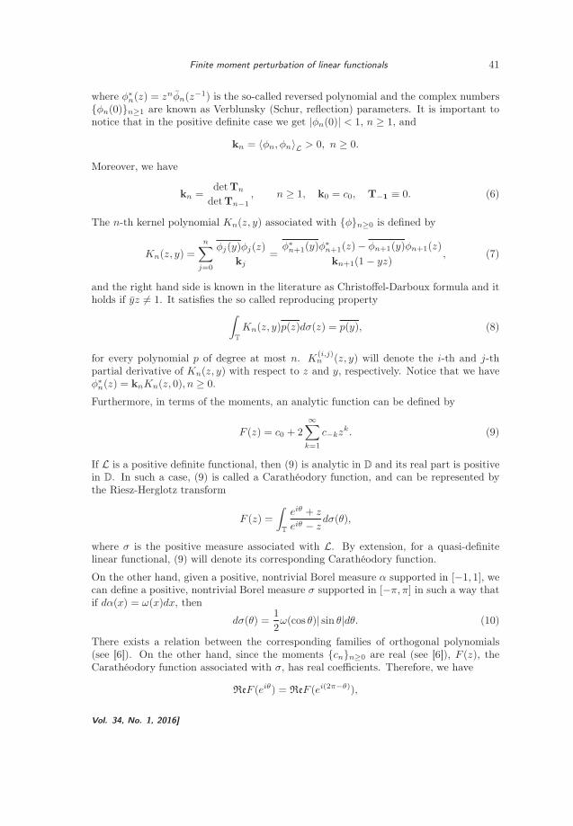
where φ∗n(z) = znφn(z

−1) is the so-called reversed polynomial and the complex numbersφn(0)n≥1 are known as Verblunsky (Schur, reflection) parameters. It is important tonotice that in the positive definite case we get |φn(0)| < 1, n ≥ 1, and

kn = φn, φnL > 0, n ≥ 0.

Moreover, we have

kn =detTn

detTn−1, n ≥ 1, k0 = c0, T−1 ≡ 0. (6)

The n-th kernel polynomial Kn(z, y) associated with φn≥0 is defined by

Kn(z, y) =

n∑

j=0

φj(y)φj(z)

kj=

φ∗n+1(y)φ

∗n+1(z)− φn+1(y)φn+1(z)

kn+1(1 − yz), (7)

and the right hand side is known in the literature as Christoffel-Darboux formula and itholds if yz = 1. It satisfies the so called reproducing property

∫

T

Kn(z, y)p(z)dσ(z) = p(y), (8)

for every polynomial p of degree at most n. K(i,j)n (z, y) will denote the i-th and j-th

partial derivative of Kn(z, y) with respect to z and y, respectively. Notice that we haveφ∗n(z) = knKn(z, 0), n ≥ 0.

Furthermore, in terms of the moments, an analytic function can be defined by

F (z) = c0 + 2

∞∑

k=1

c−kzk. (9)

If L is a positive definite functional, then (9) is analytic in D and its real part is positivein D. In such a case, (9) is called a Carathéodory function, and can be represented bythe Riesz-Herglotz transform

F (z) =

∫

T

eiθ + z

eiθ − zdσ(θ),

where σ is the positive measure associated with L. By extension, for a quasi-definitelinear functional, (9) will denote its corresponding Carathéodory function.

On the other hand, given a positive, nontrivial Borel measure α supported in [−1, 1], wecan define a positive, nontrivial Borel measure σ supported in [−π, π] in such a way thatif dα(x) = ω(x)dx, then

dσ(θ) =1

2ω(cos θ)| sin θ|dθ. (10)

There exists a relation between the corresponding families of orthogonal polynomials(see [6]). On the other hand, since the moments cnn≥0 are real (see [6]), F (z), theCarathéodory function associated with σ, has real coefficients. Therefore, we have

ReF (eiθ) = ReF (ei(2π−θ)),

Vol. 34, No. 1, 2016]


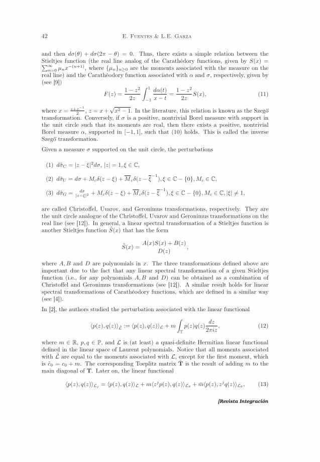
and then dσ(θ) + dσ(2π − θ) = 0. Thus, there exists a simple relation between theStieltjes function (the real line analog of the Carathédory functions, given by S(x) =∑∞

n=0 µnx−(n+1), where µnn≥0 are the moments associated with the measure on the

real line) and the Carathéodory function associated with α and σ, respectively, given by(see [9])

F (z) =1− z2

2z

∫ 1

−1

dα(t)

x− t=

1− z2

2zS(x), (11)

where x = z+z−1

2 , z = x+√x2 − 1. In the literature, this relation is known as the Szeg´o

transformation. Conversely, if σ is a positive, nontrivial Borel measure with support inthe unit circle such that its moments are real, then there exists a positive, nontrivialBorel measure α, supported in [−1, 1], such that (10) holds. This is called the inverseSzeg´o transformation.

Given a measure σ supported on the unit circle, the perturbations

(1) dσC = |z − ξ|2dσ, |z| = 1, ξ ∈ C,

(2) dσU = dσ +Mcδ(z − ξ) +M cδ(z − ξ−1

), ξ ∈ C− 0,Mc ∈ C,

(3) dσG = dσ|z−ξ|2 +Mcδ(z − ξ) +Mcδ(z − ξ

−1), ξ ∈ C− 0,Mc ∈ C, |ξ| = 1,

are called Christoffel, Uvarov, and Geronimus transformations, respectively. They arethe unit circle analogue of the Christoffel, Uvarov and Geronimus transformations on thereal line (see [12]). In general, a linear spectral transformation of a Stieltjes function isanother Stieltjes function S(x) that has the form

S(x) =A(x)S(x) +B(z)

D(z),

where A,B and D are polynomials in x. The three transformations defined above areimportant due to the fact that any linear spectral transformation of a given Stieltjesfunction (i.e., for any polynomials A,B and D) can be obtained as a combination ofChristoffel and Geronimus transformations (see [12]). A similar result holds for linearspectral transformations of Carathéodory functions, which are defined in a similar way(see [4]).

In [2], the authors studied the perturbation associated with the linear functional

p(z), q(z)L := p(z), q(z)L +m

∫

T

p(z)q(z)dz

2πiz, (12)

where m ∈ R, p, q ∈ P, and L is (at least) a quasi-definite Hermitian linear functionaldefined in the linear space of Laurent polynomials. Notice that all moments associatedwith L are equal to the moments associated with L, except for the first moment, whichis c0 = c0 + m. The corresponding Toeplitz matrix T is the result of adding m to themain diagonal of T. Later on, the linear functional

p(z), q(z)Lj= p(z), q(z)L +mzjp(z), q(z)Lθ

+ mp(z), zjq(z)Lθ, (13)



where j ∈ N is fixed and ·, ·Lθis the bilinear functional associated with the normalized

Lebesgue measure on the unit circle was studied in [3]. It is easily seen that the momentsassociated with Lj are equal to those of L, except for the moments of order j and −j,which are perturbed by adding m and m, respectively. In other words, the correspon-ding Toeplitz matriz is perturbed on the j-th and −j-th subdiagonals. In both cases,the authors obtained the regularity conditions for such a linear functional and deducedconnection formulas between the corresponding orthogonal sequences.

Assuming that both L and Lj are positive definite, the perturbation (13) can be expressedin terms of the corresponding measures as

dσ = dσ +mzjdθ

2π+ mz−j dθ

2π. (14)

On the other hand, the connection between the measure (14) and its correspondingmeasure supported in [−1, 1] via the inverse Szeg´o transformation was analyzed in [5],and it is deduced that the perturbed moments on the real line depend on the Chebyshevpolynomials of the first kind.

In this contribution, we will extend those results to the case where a perturbation of afinite number of moments is introduced in (13). In Section 2, necessary and sufficientconditions for the regularity of the perturbed functional are obtained, as well as a connec-tion formula that relates the corresponding families of monic orthogonal polynomials.For the positive definite case, the study of the perturbation through the inverse Szeg´otransformation will be analyzed in Section 3. An illustrative example will be presentedin Section 4.

2. A perturbation on a finite number of moments associated with alinear functional L

Let L be a quasi-definite linear functional on the linear space of Laurent polynomials,and let cnn∈Z be its associated sequence of moments.

Definition 2.1. Let Ω be a finite set of non negative integers. The linear functional LΩ

is defined such that the associated bilinear functional satisfies

p(z), q(z)LΩ = p(z), q(z)L +

r∈Ω

Mrzrp(z), q(z)Lθ

+M rp(z), zrq(z)Lθ

, (15)

where Mr ∈ C, p, q ∈ P, and ·, ·Lθis the bilinear functional associated with the nor-

malized Lebesgue measure in the unit circle.

Notice that, from (15), one easily sees that

cn = LΩ, zn = zn, 1LΩ =

cn, if n /∈ Ω,

c−n +M−n, if n ∈ Ω and n ∈ Z−,

cn +Mn, if n ∈ Ω and n /∈ Z−.

(16)

Vol. 34, No. 1, 2016]


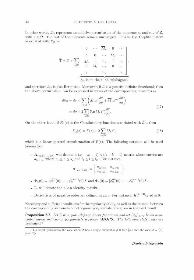
In other words, LΩ represents an additive perturbation of the moments cr and c−r of L,with r ∈ Ω. The rest of the moments remain unchanged. This is, the Toeplitz matrixassociated with LΩ is

T = T+

r∈Ω

0 · · · Mr 0 · · ·... 0 · · · M r · · ·

Mr

.... . .

.... . .

0 Mr · · · 0 · · ·...

.... . .

.... . .

,

Mr is on the r−th subdiagonal

and therefore LΩ is also Hermitian. Moreover, if L is a positive definite functional, thenthe above perturbation can be expressed in terms of the corresponding measures as

dσΩ = dσ +

r∈Ω

Mrz

r dθ

2π+M rz

−r dθ

2π

= dσ + 2

r∈Ω

Re(Mrzr)dθ

2π.

(17)

On the other hand, if FΩ(z) is the Carathéodory function associated with LΩ, then

FΩ(z) = F (z) + 2

r∈Ω

Mrzr, (18)

which is a linear spectral transformation of F (z). The following notation will be usedhereinafter:

A(s1,s2;l1,l2;r) will denote a (s2 − s1 + 1) × (l2 − l1 + 1) matrix whose entries area(s,l)r , where s1 ≤ s ≤ s2 and l1 ≤ l ≤ l2,. For instance,

A(2,3;4,5;6) =

a(2,4)6 a(2,5)6a(3,4)6 a(3,5)6

.

Ψn(0) = [ψ(0)n (0), · · · , ψ(n−1)

n (0)]T and Φn(0) = [φ(0)n (0), · · · , φ(n−1)

n (0)]T .

In will denote the n× n identity matrix.

Derivatives of negative order are defined as zero. For instance, K(0,−2)n (z, y) ≡ 0.

Necessary and sufficient conditions for the regularity of LΩ, as well as the relation betweenthe corresponding sequences of orthogonal polynomials, are given in the next result.

Proposition 2.2. Let L be a quasi-definite linear functional and let φnn≥0 be its asso-ciated monic orthogonal polynomials sequence (MOPS). The following statements areequivalent 1

1This result generalizes the case when Ω has a single element k = 0 (see [3]) and the case Ω = 0(see [2]).



1. LΩ is a quasi-definite linear functional.

2. The matrix In +

r∈Ω Srn is nonsingular, and

kn = kn + (QnWn)T

r∈Ω

Yrn +

r∈Ω

M rφ(n−r)n (0)

(n− r)!= 0, n ≥ 0, (19)

with

Yrn =

Mrφ(r)n (0)0!r!...

Mrφ(2r−1)n (0)

(r−1)!(2r−1)!

Mrφ(2r)n (0)r!(2r)! +Mr

φ(0)n (0)r!0!

...

Mrφ(n)n (0)

(n−r)!(n)! +M rφ(n−2r)n (0)

(n−r)!(n−2r)!

M rφ(n−2r+1)n (0)

(n−r+1)!(n−2r+1)!

...

Mrφ(n−r−1)n (0)

(n−1)!(n−r−1)!

, (20)

Qn = (In +

r∈Ω

Srn)

−1,

Wn = Φn(0)−

r∈Ω

M rn!C(0,n−1;n,n;r),

Krn−1(z, 0) =

MrK

(0,r)n−1 (z,0)

0!r!...

MrK

(0,2r−1)n−1 (z,0)

(r−1)!(2r−1)!

MrK

(0,2r)n−1 (z,0)

r!(2r)! +M rK

(0,0)n−1 (z,0)

r!0!

...

MrK

(0,n−1)n−1 (z,0)

(n−r−1)!(n−1)! +MrK

(0,n−2r−1)n−1 (z,0)

(n−r−1)!(n−2r−1)!

M rK

(0,n−2r)n−1 (z,0)

(n−r)!(n−2r)!

...

M rK

(0,n−r−1)n−1 (z,0)

(n−1)!(n−r−1)! .

, (21)

Vol. 34, No. 1, 2016]


and

Srn =

MrA(0,r−1;0,r−1;r) B(0,r−1;r,n−r−1;r) MrC(0,r−1;n−r,n−1;r)

MrA(r,n−r−1;0,r−1;r) B(r,n−r−1;r,n−r−1;r) M rC(r,n−r−1;n−r,n−1;r)

MrA(n−r,n−1;0,r−1;r) B(n−r,n−1;r,n−r−1;r) M rC(n−r,n−1;n−r,n−1;r)

,

where the entries of the matrices A, B and C are given by

a(s,l)r =K

(s,l+r)n−1 (0, 0)

l!(l+ r)!,

b(s,l)r = Mr

K(s,l+r)n−1 (0, 0)

l!(l+ r)!+Mr

K(s,l−r)n−1 (0, 0)

l!(l− r)!,

c(s,l)r =K

(s,l−r)n−1 (0, 0)

l!(l− r)!.

Furthermore, if ψnn≥0 denotes the MOPS associated with LΩ, then

ψn(z) = φn(z)− (QnWn)T

r∈Ω

Krn−1(z, 0)−

r∈Ω

M r

K(0,n−r)n−1 (z, 0)

(n− r)!, (22)

for every n ≥ 1.

Remark 2.3. Notice that Qn and Srn are n×n matrices, whereas Yr

n,Wn and Krn−1(z, 0)

are n-th dimensional column vectors.

Proof. Assume LΩ is a quasi-definite linear functional, and denote by ψnn≥0 its asso-ciated MOPS. Let us write

ψn(z) = φn(z) +

n−1

k=0

λn,kφk(z), (23)

where, for 0 ≤ k ≤ n− 1,

λn,k =ψn(z), φk(z)L

kn

=ψn(z), φk(z)LΩ −

r∈Ω Mr

Tyrψn(y)φk(y)

dy2πiy −

r∈Ω M r

Ty−rψn(y)φk(y)

dy2πiy

kk

= −

r∈Ω

Mr

kk

T

yrψn(y)φk(y)dy

2πiy−

r∈Ω

M r

kk

T

y−rψn(y)φk(y)dy

2πiy,

and notice that ψn(z), φk(z)L = 0 (in general), and ψn(z), φk(z)LΩ = 0 for n > k.



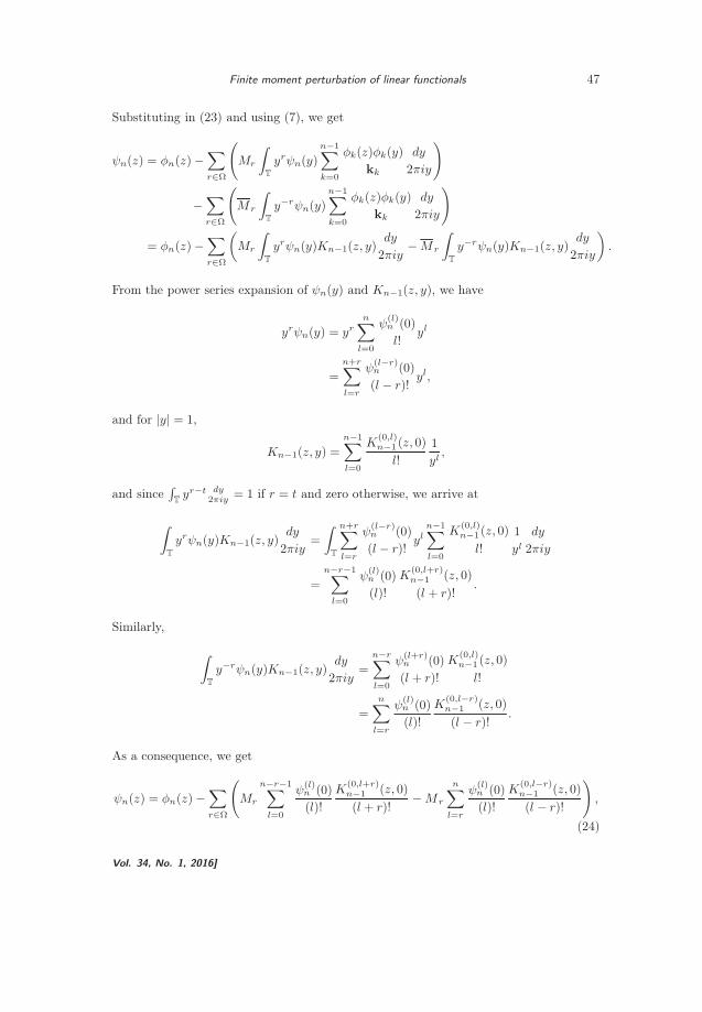
Substituting in (23) and using (7), we get

ψn(z) = φn(z)−∑

r∈Ω

(Mr

∫

T

yrψn(y)

n−1∑

k=0

φk(z)φk(y)

kk

dy

2πiy

)

−∑

r∈Ω

(M r

∫

T

y−rψn(y)

n−1∑

k=0

φk(z)φk(y)

kk

dy

2πiy

)

= φn(z)−∑

r∈Ω

(Mr

∫

T

yrψn(y)Kn−1(z, y)dy

2πiy−M r

∫

T

y−rψn(y)Kn−1(z, y)dy

2πiy

).

From the power series expansion of ψn(y) and Kn−1(z, y), we have

yrψn(y) = yrn∑

l=0

ψ(l)n (0)

l!yl

=

n+r∑

l=r

ψ(l−r)n (0)

(l − r)!yl,

and for |y| = 1,

Kn−1(z, y) =

n−1∑

l=0

K(0,l)n−1 (z, 0)

l!

1

yl,

and since∫Tyr−t dy

2πiy = 1 if r = t and zero otherwise, we arrive at

∫

T

yrψn(y)Kn−1(z, y)dy

2πiy=

∫

T

n+r∑

l=r

ψ(l−r)n (0)

(l − r)!yl

n−1∑

l=0

K(0,l)n−1(z, 0)

l!

1

yldy

2πiy

=

n−r−1∑

l=0

ψ(l)n (0)

(l)!

K(0,l+r)n−1 (z, 0)

(l + r)!.

Similarly,

∫

T

y−rψn(y)Kn−1(z, y)dy

2πiy=

n−r∑

l=0

ψ(l+r)n (0)

(l + r)!

K(0,l)n−1 (z, 0)

l!

=

n∑

l=r

ψ(l)n (0)

(l)!

K(0,l−r)n−1 (z, 0)

(l − r)!.

As a consequence, we get


r∈Ω

(Mr

n−r−1∑

l=0

ψ(l)n (0)

(l)!

K(0,l+r)n−1 (z, 0)

(l + r)!−M r

n∑

l=r

ψ(l)n (0)

(l)!

K(0,l−r)n−1 (z, 0)

(l − r)!

),

(24)

Vol. 34, No. 1, 2016]


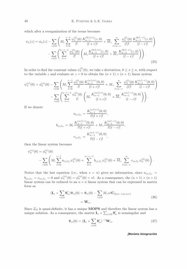
which after a reorganization of the terms becomes


r∈Ω

(Mr

r−1∑

l=0

ψ(l)n (0)

l!

K(0,l+r)n−1 (z, 0)

(l + r)!+Mr

n∑

l=n−r

ψ(l)n (0)

(l)!

K(0,l−r)n−1 (z, 0)

(l − r)!

)

−∑

r∈Ω

(n−r−1∑

l=r

ψ(l)n (0)

l!

(Mr

K(0,l+r)n−1 (z, 0)

(l + r)!+M r

K(0,l−r)n−1 (z, 0)

(l − r)!

)).

(25)

In order to find the constant values ψ(l)n (0), we take s derivatives, 0 ≤ s ≤ n, with respect

to the variable z and evaluate at z = 0 to obtain the (n+ 1)× (n+ 1) linear system

ψ(s)n (0) = φ(s)

n (0)−∑

r∈Ω

(Mr

r−1∑

l=0

ψ(l)n (0)

l!

K(s,l+r)n−1 (0, 0)

(l + r)!+Mr

n∑

l=n−r

ψ(l)n (0)

(l)!

K(s,l−r)n−1 (0, 0)

(l − r)!

)

−∑

r∈Ω

(n−r−1∑

l=r

ψ(l)n (0)

l!

(Mr

K(s,l+r)n−1 (0, 0)

(l + r)!+M r

K(s,l−r)n−1 (0, 0)

(l − r)!

)).

If we denote

a(s,l)r =K

(s,l+r)n−1 (0, 0)

l!(l + r)!,

b(s,l)r = Mr

K(s,l+r)n−1 (0, 0)

l!(l+ r)!+M r

K(s,l−r)n−1 (0, 0)

l!(l − r)!,

c(s,l)r =K

(s,l−r)n−1 (0, 0)

l!(l − r)!,

then the linear system becomes

ψ(s)n (0) = φ(s)

n (0)

−∑

r∈Ω

(Mr

r−1∑

l=0

a(s,l)rψ(l)n (0) +

n−r−1∑

l=r

b(s,l)rψ(l)n (0) +Mr

n∑

l=n−r

c(s,l)rψ(l)n (0)

).

Notice that the last equation (i.e., when s = n) gives no information, since a(n,l)r =

b(n,l)r = c(n,l)r = 0 and ψ(n)n (0) = φ

(n)n (0) = n!. As a consequence, the (n+ 1)× (n+ 1)

linear system can be reduced to an n× n linear system that can be expressed in matrixform as

(In +∑

r∈Ω

Srn)Ψn(0) = Φn(0)−

∑

r∈Ω

M rn!C(0,n−1;n,n;r)

= Wn.

(26)

Since LΩ is quasi-definite, it has a unique MOPS and therefore the linear system has aunique solution. As a consequence, the matrix In +

∑r∈Ω Sr

n is nonsingular and

Ψn(0) = (In +∑

r∈Ω

Srn)

−1Wn. (27)



This is, we have

ψn(z) = φn(z)−

r∈Ω

WTn

(In +

r∈Ω

Srn)

−1

T

Krn−1(z, 0)−

r∈Ω

Mr

K(0,n−r)n−1 (z, 0)

(n− r)!, (28)

which is (22). On the other hand, for n ≥ 0,

kn = ψn(z), ψn(z)LΩ = ψn(z), φn(z)LΩ

= ψn(z), φn(z)L +

r∈Ω

Mrzrψn(z), φn(z)Lθ

+Mrψn(z), zrφn(z)Lθ

= kn +

r∈Ω

Mr

T

n

l=0

ψ(l)n (0)

l!zl+r

n

l=0

φ(l)n (0)

l!z−l dz

2πiz

+

r∈Ω

Mr

T

n

l=0

ψ(l)n (0)

l!zl−r

n

l=0

φ(l)n (0)

l!z−l dz

2πiz

= kn +

r∈Ω

Mr

r−1

l=0

ψ(l)n (0)

l!

φ(l+r)n (0)

(l + r)!+

n−r

l=r

ψ(l)n (0)

l!

Mrφ(l+r)n (0)

(l + r)!+M r

φ(l−r)n (0)

(l − r)!

+

r∈Ω

Mr

n−1

l=n−r+1

ψ(l)n (0)

l!

φ(l−r)n (0)

(l − r)!

+

r∈Ω

M rφ(n−r)n (0)

(n− r)!.

Using (20) and (27), we get

kn = kn +

r∈Ω

WTn

(In +

r∈Ω

Srn)

−1

T

Yrn +

r∈Ω

M rφ(n−r)n (0)

(n− r)!.

Conversely, assume In +

r∈Ω Srn is nonsingular for every n ≥ 1 and define ψnn≥0 as

in (22). For 0 ≤ k ≤ n− 1, we have

n−r−1

l=0

ψ(l)n (0)

l!

K(0,l+r)n−1 (z, 0)

(l + r)!, φk(z)

L

=n−r−1

l=0

ψ(l)n (0)

l!

K(0,l+r)n−1 (z, 0)

(l + r)!, φk(z)

L

=n−r−1

l=0

ψ(l)n (0)

l!(l + r)!

n−1

t=0

φt(z)φ(l+r)t (0)

kt, φk(z)

L

=

n−r−1

l=0

ψ(l)n (0)

l!

φ(l+r)k (0)

(l + r)!,

and, similarly,

n

l=j

ψ(l)n (0)

l!

K(0,l−r)n−1 (z, 0)

(l − r)!, φk(z)

L

=n

l=r

ψ(l)n (0)

l!

φ(l−r)k (0)

(l − r)!.

Vol. 34, No. 1, 2016]


In addition,

zrψn(z), φk(z)Lθ=

T

zrψn(z)φk(z)dz

2πiz

=

T

zr

n

l=0

ψ(l)n (0)zl

l!

k

l=0

φ(l)n (0)z−l

l!

dz

2πiz

=

n−r−1

l=0

ψ(l)n (0)

l!

φ(l+r)k (0)

(l + r)!,

and also

ψn(z), zrφk(z)Lθ

=

n

l=r

ψ(l)n (0)

l!

φ(l−r)k (0)

(l − r)!.

Thus, for 0 ≤ k ≤ n − 1, and taking into account (24) and the previous equations, wehave

ψn(z), φk(z)LΩ = ψn(z), φk(z)L +

r∈Ω

Mrzrψn(z), φk(z)Lθ

+M rψn(z), zrφk(z)Lθ

= φn(z), φn(z)L −

r∈Ω

Mr

n−r−1

l=0

ψ(l)n (0)

(l)!

K(0,l+r)n−1 (z, 0)

(l + r)!, φk(z)

L

−

r∈Ω

M r

n

l=r

ψ(l)n (0)

(l)!

K(0,l−r)n−1 (z, 0)

(l − r)!, φk(z)

L

+

r∈Ω

Mr

n−r−1

l=0

ψ(l)n (0)

l!

φ(l+r)k (0)

(l + r)!

+

r∈Ω

Mr

n

l=r

ψ(l)n (0)

l!

φ(l−r)k (0)

(l − r)!

= 0.

On the other hand,

kn = ψn(z), φn(z)LΩ

= ψn(z), φn(z)L +

r∈Ω

Mrzrψn(z), φn(z)Lθ

+Mrψn(z), zrφn(z)Lθ

= kn +

r∈Ω

Mr

T

n

l=0

ψ(l)n (0)

l!zl+r

n

l=0

φ(l)n (0)

l!z−l dz

2πiz

+

r∈Ω

M r

T

n

l=0

ψ(l)n (0)

l!zl−r

n

l=0

φ(l)n (0)

l!z−l dz

2πiz

= kn +

r∈Ω

ΨTn (0)Y

rn(0) +

r∈Ω

Mrφ(n−r)n (0)

(n− r)!,

which is different from 0 by assumption. Therefore, LΩ is quasi-definite.



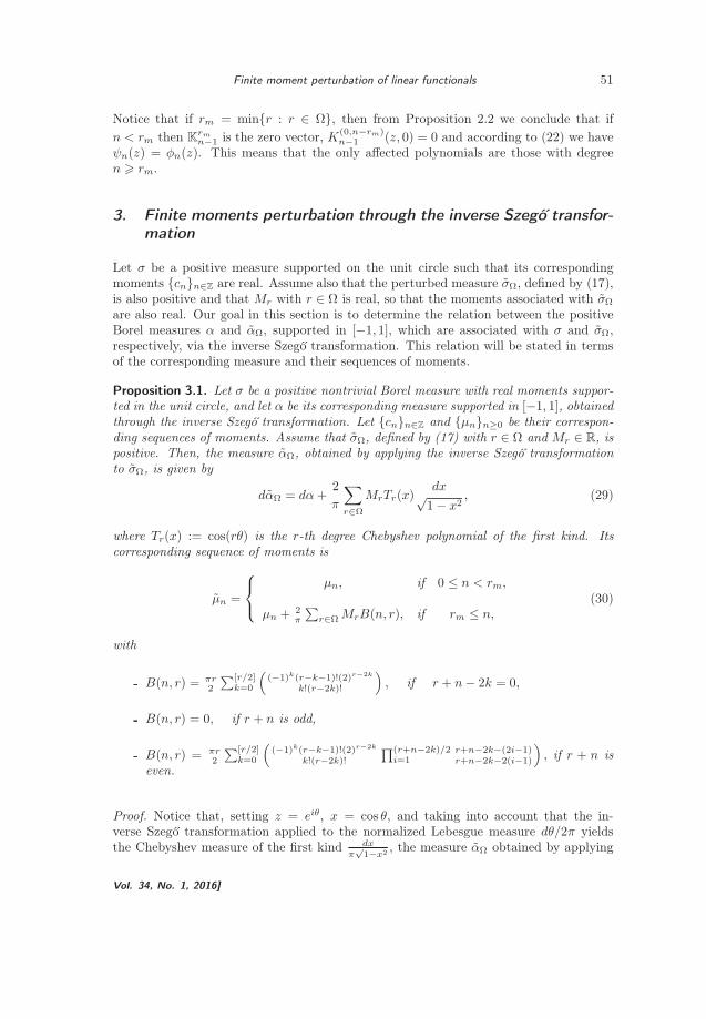
Notice that if rm = minr : r ∈ Ω, then from Proposition 2.2 we conclude that if

n < rm then Krmn−1 is the zero vector, K

(0,n−rm)n−1 (z, 0) = 0 and according to (22) we have

ψn(z) = φn(z). This means that the only affected polynomials are those with degreen rm.

3. Finite moments perturbation through the inverse Szegó transfor-mation

Let σ be a positive measure supported on the unit circle such that its correspondingmoments cnn∈Z are real. Assume also that the perturbed measure σΩ, defined by (17),is also positive and that Mr with r ∈ Ω is real, so that the moments associated with σΩ

are also real. Our goal in this section is to determine the relation between the positiveBorel measures α and αΩ, supported in [−1, 1], which are associated with σ and σΩ,respectively, via the inverse Szegó transformation. This relation will be stated in termsof the corresponding measure and their sequences of moments.

Proposition 3.1. Let σ be a positive nontrivial Borel measure with real moments suppor-ted in the unit circle, and let α be its corresponding measure supported in [−1, 1], obtainedthrough the inverse Szego transformation. Let cnn∈Z and µnn≥0 be their correspon-ding sequences of moments. Assume that σΩ, defined by (17) with r ∈ Ω and Mr ∈ R, ispositive. Then, the measure αΩ, obtained by applying the inverse Szego transformationto σΩ, is given by

dαΩ = dα+2

π

r∈Ω

MrTr(x)dx√1− x2

, (29)

where Tr(x) := cos(rθ) is the r-th degree Chebyshev polynomial of the first kind. Itscorresponding sequence of moments is

µn =

µn, if 0 ≤ n < rm,

µn + 2π

r∈Ω MrB(n, r), if rm ≤ n,

(30)

with

B(n, r) = πr2

[r/2]k=0

(−1)k(r−k−1)!(2)r−2k

k!(r−2k)!

, if r + n− 2k = 0,

B(n, r) = 0, if r + n is odd,

B(n, r) = πr2

[r/2]k=0

(−1)k(r−k−1)!(2)r−2k

k!(r−2k)!

(r+n−2k)/2i=1

r+n−2k−(2i−1)r+n−2k−2(i−1)

, if r + n is

even.

Proof. Notice that, setting z = eiθ, x = cos θ, and taking into account that the in-verse Szegó transformation applied to the normalized Lebesgue measure dθ/2π yieldsthe Chebyshev measure of the first kind dx

π√1−x2

, the measure αΩ obtained by applying

Vol. 34, No. 1, 2016]


the inverse Szeg´o transformation to σΩ is given by

dαΩ = dα+

r∈Ω

Mr(x+ i

1− x2)r +Mr(x+ i

1− x2)−r

dx

π√1− x2

= dα+

r∈Ω

(Mr(cos rθ + i sin rθ) +Mr(cos rθ − i sin rθ))dx

π√1− x2

= dα+2

π

r∈Ω

MrTr(x)dx√1− x2

.

Notice that a measure that changes its sign in the interval [−1, 1] is added to dα. Then,the moments associated with αΩ are given by

µn =

1

−1

xndαΩ(x) = µn +2

π

r∈Ω

Mr

1

−1

xn Tr(x)dx√1− x2

.

As a consequence, by the orthogonality of Tr(x), we obtain for the n-th moments withn /∈ Ω

µn =

µn, if 0 ≤ n < rm,

µn + 2π

r∈ΩMr

1

−1xn Tr(x)dx√

1−x2, if rm ≤ n.

(31)

Furthermore (see [8]), we have

Tr(x) =r

2

[r/2]

k=0

(−1)k(r − k − 1)!(2x)r−2k

k!(r − 2k)!, r = 1, 2, 3, ...,

where [r/2] = r/2 if r is even and [r/2] = (r − 1)/2 if r is odd. Therefore,

1

−1

xnTr(x)dx√1− x2

=r

2

1

−1

xn

[r/2]

k=0

(−1)k(r − k − 1)!(2x)r−2k

k!(r − 2k)!

dx√1− x2

=r

2

[r/2]

k=0

(−1)k(r − k − 1)!(2)r−2k

k!(r − 2k)!

1

−1

xr+n−2k dx√1− x2

,

and, since

1

−1

xk dx√1− x2

=

π, if k = 0,

0, if k is odd,

k/2i=1

k−(2i−1)k−2(i−1)

π, if k is even,

(31) becomes (30).

From the previous proposition we can conclude that a perturbation of the moments crand c−r with r ∈ Ω, associated with a measure σ supported in the unit circle, resultsin a perturbation, defined by (30), of the moments µn, n rm, associated with ameasure α supported in [−1, 1], when both measures are related through the inverseSzeg´o transformation.



4. Example

Let L be the Christoffel transformation of the normalized Lebesgue measure with pa-rameter ξ = 1, i.e., p(z), q(z)L = (z − 1)p(z), (z − 1)q(z)Lθ

, and let Ω = 1, 2.Then,

p(z), q(z)L1,2= (z − 1)p(z), (z − 1)q(z)Lθ

+M1zp(z), q(z)Lθ+M1p(z), zq(z)Lθ

+M2z2p(z), q(z)Lθ+M2p(z), z2q(z)Lθ

,

(32)

i.e., the moments of order 1 and 2 are perturbed. Since the sequence znn≥0 is ortho-gonal with respect to Lθ, the MOPS associated with (z−1)p(z), (z−1)q(z)Lθ

is givenby (see [1])

φn(z) =1

z − 1

zn+1 − 1

n+ 1

n

j=0

zj

, n ≥ 1,

or, equivalently,

φn(z) = zn +n

n+ 1φn−1(z), n ≥ 1,

and its corresponding reversed polynomial is

φ∗n(z) =

1

1− z

1− 1

n+ 1

n

j=0

zj+1

, n ≥ 1.

Furthermore, if 0 ≤ s ≤ n, we have

φ(s)n (0) =

(s+ 1)!

(n+ 1),

φ∗(s)n (0) =

s!(n+ 1− s)

(n+ 1),

kn =n+ 2

n+ 1,

and if 0 ≤ t, s ≤ n− 1,

K(0,t)n−1 (z, 0) =

n−1

p=t

(t+ 1)!

p+ 2φp(z),

K(s,t)n−1 (0, 0) =

n−1

p=maxs,t

(t+ 1)!(s+ 1)!

(p+ 1)(p+ 2).

As a consequence, we have

a(s,l)r =(s+ 1)!(l + r + 1)

l!

n−1

p=maxs,l+r

1

(p+ 1)(p+ 2),

Vol. 34, No. 1, 2016]


c(s,l)r =(s+ 1)!(l − r + 1)

l!

n−1

p=maxs,l−r

1

(p+ 1)(p+ 2),

b(s,l)r =(s+ 1)!

l!

Mr

n−1

p=maxs,l+r

l + r + 1

(p+ 1)(p+ 2)+Mr

n−1

p=maxs,l−r

l − r + 1

(p+ 1)(p+ 2)

.

We now proceed to obtain the MOPS associated with L1,2, denoted by ψnn≥0.

Notice that we have c(s,n)1 = (s+1)!n!(n+1) , c(s,n)2 = 2(s+1)!

n!(n+1) if 0 ≤ s ≤ n− 2 and c(n−1,n)2 =n−1

n(n+1) , and thus

Wn =

φ(0)n (0)

φ(1)n (0)

...

φ(n−2)n (0)

φ(n−1)n (0)

−M1n!

c(0,n)1c(1,n)1

...c(n−2,n)1

c(n−1,n)1

−M2n!

c(0,n)2c(1,n)2

...c(n−2,n)2

c(n−1,n)2

=1−M1

n+ 1

1!2!...

(n− 1)!n!

− 2M2

n+ 1

1!2!...

(n− 1)!n!n−1

2n

.

On the other hand, for n ≥ 2 we have

K1n−1(z, 0) =

2M1

n−1p=1

φp(z)p+2

3M1

n−1p=2

φp(z)p+2 +M1

n−1p=0

φp(z)p+2

...nM1

(n−2)!

n−1p=n−1

φp(z)p+2 + M1

(n−3)!

n−1p=n−3

φp(z)p+2

M1

(n−2)!

n−1p=n−2

φp(z)p+2

,

S1n =

M1a(0,0)1 b(0,1)1 · · · b(0,n−2)1 M1c(0,n−1)1

M1a(1,0)1 b(1,1)1 · · · b(1,n−2)1 M1c(1,n−1)1...

.... . .

......

M1a(n−2,0)1 b(n−2,1)1 · · · b(n−2,n−2)1 M1c(n−2,n−1)1

M1a(n−1,0)1 b(n−1,1)1 · · · b(n−1,n−2)1 M1c(n−1,n−1)1

,



and for n ≥ 3,

K2n−1(z, 0) =

3M2

n−1p=2

φp(z)p+2

4M2

n−1p=3

φp(z)p+2

5M2

2

n−1p=4

φp(z)p+2 + M2

2

n−1p=0

φp(z)p+2

...nM2

(n−3)!

n−1p=n−1

φp(z)p+2 + M2

(n−3)(n−5)!

n−1p=n−5

φp(z)p+2

M2

(n−2)(n−4)!

n−1p=n−4

φp(z)p+2

M2

(n−1)(n−3)!

n−1p=n−3

φp(z)p+2

,

S2n =

M2a(0,0)2 M2a(0,1)2 b(0,2)2 · · · b(0,n−3)2 M2c(0,n−2)2 M2c(0,n−1)2

M2a(1,0)2 M2a(1,1)2 b(1,2)2 · · · b(1,n−3)2 M2c(1,n−2)2 M2c(1,n−1)2

M2a(2,0)2 M2a(2,1)2 b(2,2)2 · · · b(2,n−3)2 M2c(2,n−2)2 M2c(2,n−1)2

......

.... . .

......

...

M2a(n−3,0)2 M2a(n−3,1)2 b(n−3,2)2 · · · b(n−3,n−3)2 M2c(n−3,n−2)2 M2c(n−3,n−1)2



,

For illustrative purposes, we compute the first polynomials of the sequence:

Degree one:

ψ1(z) = φ1(z)−M1K

(0,0)0 (z, 0)

0!

= z +(1−M1)

2φ0(z),

since K10(z, 0) = 0, K2

0(z, 0) = 0 and φ1(z) = z + 12φ0(z).

Vol. 34, No. 1, 2016]


Degree two:

ψ2(z) = φ2(z)

−

1−M1

3

1!2!

T

−

2M2

3

1!12

T

M13

+ 1 2M13

2M13

M13

+ 1

−1

T

2M13

φ1(z)

M1

φ0(z)2

+ φ1(z)3

−

2M1

3φ1(z)−M2

φ0(z)

2+

φ1(z)

3

= z2 +1−M1

3

2φ1(z)− A

1!2!

T

M13

+ 1 −2M13

−2M13

M13

+ 1

2M13

φ1(z)

M1

φ0(z)2

+ φ1(z)3

−M2

φ0(z)

2+

φ1(z)

3−

2

3A

1!12

T

M13

+ 1 −2M13

−2M13

M13

+ 1

2M13

φ1(z)

M1

φ0(z)2

+ φ1(z)3

,

since K21(z, 0) = 0, φ2(z) = z2 + 2

3φ1(z) and A = 1

det(I2+S12+S2

2)= 9

|M1+3|2−4|M1|2.

In general, the n-th degree polynomial is

ψn(z) = φn(z)−

1−M1

n+ 1

1!2!...

(n− 1)!n!

T

−

2M2

n+ 1

1!2!...

(n− 1)!n!(n− 1)/2n

T

(In +2

r=1

Srn)

−1

T

×

2

r=1

Krn−1(z, 0)

−

nM1

n+ 1φn−1(z)−M2(n− 1)

φn−2(z)

n+

φn−1(z)

n+ 1

= zn +1−M1

n+ 1

nφn−1(z)−

1!2!...

(n− 1)!n!

T

(In +2

r=1

Srn)

−1

T

2

r=1

Krn−1(z, 0)

−M2(n− 1)

φn−1(z)

n+ 1+

φn−2(z)

n

+2M2

n+ 1

1!2!...

(n− 1)!n!n−1

2n

T

(In +

2

r=1

Srn)

−1

T

2

r=1

Krn−1(z, 0)

,

since φn(z) = zn + n

n+1φn−1(z).

On the other hand, assuming that the linear functional (32) is positive definite, theassociated measure is

dσ = |z − 1|2 dθ2π

+ 2Re(M1z)dθ

2π+ 2Re(M2z

2)dθ

2π,



and the corresponding moments are given by

cn =

2, if n = 0,−1 +M1, if n = 1,−1 +M1, if n = −1,

M2, if n = 2,M2, if n = −2,0, in other case.

Thus, the perturbed Toeplitz matrix is

T =

2 −1 +M1 M2 0 0 · · ·−1 +M1 2 −1 +M1 M2 0 · · ·

M2 −1 +M1 2 −1 +M1 M2 · · ·0 M2 −1 +M1 2 −1 +M1 · · ·0 0 M2 −1 +M1 2 · · ·...

......

......

. . .

,

i.e., the first and second subdiagonals are perturbed. Furthermore, since dα = 2π

1−x1+xdx

is the measure obtained applying the inverse Szeg´o transformation to dσ = |z − 1|2 dθ2π ,

then according to (29) the measure supported in [−1, 1] is

dα =2

π

1− x

1 + xdx+

2

πM1T1(x)

1√1− x2

dx+2

πM2T2(x)

1√1− x2

dx. (33)

Then, according to (30), the perturbed moments associated with the measure (33) are

µn =

µn, if n = 0,

µn + 2M1

n+12

i=1n+1−(2i−1)n+1−2(i−1) , if n is odd,

µn + 2M2

2n+2

2i=1

n+2−(2i−1)n+2−2(i−1) −

n2i=1

n−(2i−1)n−2(i−1)

, if n is even,

where µnn≥0 are the moments associated with the measure dα = 2π

1−x1+x , and

µn =

2, if n = 0,

−2n+1

2

i=1n+1−(2i−1)n+1−2(i−1) , if n is odd,

2n

2

i=1n−(2i−1)n−2(i−1) , if n is even.

Acknowledgements

The work of the second author was supported by Consejo Nacional de Ciencia y Tec-nología of México, grant 156668. Both authors thank the anonymous referees for her/hisvaluable comments and suggestions. They contributed greatly to improve the presenta-tion and contents of the manuscript.

Vol. 34, No. 1, 2016]


References

[1] Bueno M.I. and Marcellán F., “Polynomial perturbations of bilinear functionals and Hessen-berg matrices”, Linear Algebra Appl. 414 (2006), No. 1, 64–83.

[2] Castillo K., Garza L.E. and Marcellán F., “Linear spectral transformations, Hessenbergmatrices and orthogonal polynomials”, Rend. Circ. Mat. Palermo (2) Suppl. (2010), No.82, 3–26.

[3] Castillo K., Garza L.E. and Marcellán F., “Perturbations on the subdiagonals of Toeplitzmatrices”, Linear Algebra Appl. 434 (2011), No. 6, 1563–1579.

[4] Castillo K. and Marcellán F., “Generators of rational spectral transformations for nontrivialC-functions”, Math. Comp. 82 (2013), No. 282, 1057–1068.

[5] Fuentes E. and Garza L.E., “Analysis of perturbations of moments associated with ortho-gonality linear functionals through the Szego transformation”, Rev. Integr. Temas Mat. 33(2015), No. 1, 61–82.

[6] Garza L., Hernández J. and Marcellán F., “Spectral transformations of measures supportedon the unit circle and the Szego transformation”, Numer. Algorithms. 49 (2008), No. 1-4,169–185.

[7] Grenander U. and Szego G., Toeplitz forms and their applications, Second ed., ChelseaPublishing Co., New York, 1984.

[8] Kreyszig E., Introductory functional analysis with applications, John Wiley & Sons Inc.,New York, 1989.

[9] Peherstorfer F., “A special class of polynomials orthogonal on the circle including theassociated polynomials”, Constr. Approx. 12 (1996), No. 2, 161–185.

[10] Simon B., Orthogonal polynomials on the unit circle. Part 1 and 2, American MathematicalSociety Colloquium Publications 54, American Mathematical Society, Providence, RI, 2005.

[11] Szego G., Orthogonal polynomials, Fourth ed., American Mathematical Society ColloquiumPublications 23, American Mathematical Society, Providence, RI, 1975.

[12] Zhedanov A., “Rational spectral transformations and orthogonal polynomials”, J. Comput.Appl. Math. 85 (1997), No. 1, 67–86.


redalyc.on a finite moment perturbation of linear functionals and

Documents