integral representations of positive linear functionals
TRANSCRIPT

University of Central Florida University of Central Florida
STARS STARS
Electronic Theses and Dissertations, 2004-2019
2015
Integral Representations of Positive Linear Functionals Integral Representations of Positive Linear Functionals
Angela Siple University of Central Florida
Part of the Mathematics Commons
Find similar works at: https://stars.library.ucf.edu/etd
University of Central Florida Libraries http://library.ucf.edu
This Doctoral Dissertation (Open Access) is brought to you for free and open access by STARS. It has been accepted
for inclusion in Electronic Theses and Dissertations, 2004-2019 by an authorized administrator of STARS. For more
information, please contact [email protected].
STARS Citation STARS Citation Siple, Angela, "Integral Representations of Positive Linear Functionals" (2015). Electronic Theses and Dissertations, 2004-2019. 1178. https://stars.library.ucf.edu/etd/1178

INTEGRAL REPRESENTATIONS OF POSITIVE LINEARFUNCTIONALS
by
ANGELA SIPLEB.S. University of Central Florida, 2008M.S. University of Central Florida, 2012
A dissertation submitted in partial fulfillment of the requirementsfor the degree of Doctor of Philosophyin the Department of Mathematics
in the College of Sciencesat the University of Central Florida
Orlando, Florida
Spring Term2015
Major Professor:Dragu Atanasiu, Piotr Mikusinski

c⃝ 2015 by ANGELA SIPLE
ii

ABSTRACT
In this dissertation we obtain integral representations for positive linear functionals on
commutative algebras with involution and semigroups with involution. We prove Bochner
and Plancherel type theorems for representations of positive functionals and show that,
under some conditions, the Bochner and Plancherel representations are equivalent. We also
consider the extension of positive linear functionals on a Banach algebra into a space of
pseudoquotients and give under conditions in which the space of pseudoquotients can be
identified with all Radon measures on the structure space. In the final chapter we consider a
system of integrated Cauchy functional equations on a semigroup, which generalizes a result
of Ressel and offers a different approach to the proof.
iii

TABLE OF CONTENTS
CHAPTER 1 A BERG-MASERICK TYPE THEOREM . . . . . . . . . . . . . . . 3
1.1 Introduction . . . . . . . . . . . . . . . . . . . . . . . . . . . . . . . . . . . . 3
1.2 Berg-Maserick type theorem . . . . . . . . . . . . . . . . . . . . . . . . . . . 6
CHAPTER 2 SEMIGROUP REPRESENTATIONS . . . . . . . . . . . . . . . . . . 16
2.1 Introduction . . . . . . . . . . . . . . . . . . . . . . . . . . . . . . . . . . . . 16
2.2 Semigroup Representations . . . . . . . . . . . . . . . . . . . . . . . . . . . . 17
2.3 Examples . . . . . . . . . . . . . . . . . . . . . . . . . . . . . . . . . . . . . 24
CHAPTER 3 INTEGRATED CAUCHY FUNCTIONAL EQUATION ON COMMU-
TATIVE SEMIGROUPS . . . . . . . . . . . . . . . . . . . . . . . . . . . . . . . . . . 30
3.1 Introduction . . . . . . . . . . . . . . . . . . . . . . . . . . . . . . . . . . . . 30
3.2 Defintions and Preliminary Concepts . . . . . . . . . . . . . . . . . . . . . . 32
3.3 System of Cauchy Functional Equations . . . . . . . . . . . . . . . . . . . . 34
3.4 Examples . . . . . . . . . . . . . . . . . . . . . . . . . . . . . . . . . . . . . 44
iv

CHAPTER 4 BOCHNER-PLANCHEREL THEOREMS IN ALGEBRAS WITH IN-
VOLUTION . . . . . . . . . . . . . . . . . . . . . . . . . . . . . . . . . . . . . . . . . 48
4.1 Definitions and notation . . . . . . . . . . . . . . . . . . . . . . . . . . . . . 48
4.2 Bochner-type integral representations . . . . . . . . . . . . . . . . . . . . . . 51
4.3 A Plancherel-type integral representation . . . . . . . . . . . . . . . . . . . . 58
4.4 Back to Bochner . . . . . . . . . . . . . . . . . . . . . . . . . . . . . . . . . 66
CHAPTER 5 PSEUDOQUOTIENTS ON COMMUTATIVE BANACH ALGEBRAS 70
5.1 Introduction . . . . . . . . . . . . . . . . . . . . . . . . . . . . . . . . . . . . 70
5.2 An extension of Maltese’s theorem . . . . . . . . . . . . . . . . . . . . . . . 73
5.3 Examples . . . . . . . . . . . . . . . . . . . . . . . . . . . . . . . . . . . . . 79
LIST OF REFERENCES . . . . . . . . . . . . . . . . . . . . . . . . . . . . . . . . . 82
v
INTRODUCTION
At the core of this dissertation is Bochner’s theorem. The classical Bochner’s theorem
characterizes the Fourier transforms of finite positive Radon measures on the real line as
positive definite functions. Since Bochner proved this theorem, it has been generalized and
modified in many different ways. Common to these generalizations is identification of a
space of positive definite functions on semigroups, groups, or algebras with a space of Radon
measures on a set of characters. In this dissertation we prove some known results using new,
simpler, and more elegant techniques. We also obtain some new results. Our approach can
be characterized by a direct construction of the measure rather than using Choquet’s theory
or Gelfand’s theory.
In Chapter 1 we prove an integral representation of a positive definite functional on
a commutative semigroup with involution. This type of result was first proved by Berg-
Maserick in [10]. Then it was generalized by Atanasiu in [1] and [4]. Here we present a new
proof of Atanasiu’s result.
In Chapter 2 we study semigroup representations using a direct sum of L2 spaces
without using Gelfand’s theory. Instead, we use the integral representation of positive definite
functionals from Chapter 1.
In Chapter 3 we consider a system of integrated Cauchy functional equations on a
semigroup. The original paper of Deny considers the equation σ = µ ∗ σ on locally compact
1

commutative groups. Ressel generalized this result in [24]. Here we prove an extension of
Ressel’s result. Our proof is simpler and more elementary than that of Ressel.
In Chapter 4 we find Bochner and Plancherel type integral representations of positive
functionals on a commutative algebra with involution. We also show that, under some
conditions, Plancherel representation is equivalent to a Bochner representation.
In Chapter 5 we consider pseudoquotient extensions of positive linear functionals on
a commutative Banach algebra and give conditions under which the constructed space of
pseudoquotients can be identified with all Radon measures on the structure space.
2

CHAPTER 1
A BERG-MASERICK TYPE THEOREM
1.1 Introduction
Let (S, ·) be a commutative semigroup with involution ∗ and neutral element e.
Definition 1.1.1. An involution on a semigroup is a map x 7→ x∗ from S to S such that
the following hold for all x, y ∈ S,
e∗ = e (xy)∗ = y∗x∗, (x∗)∗ = x
Definition 1.1.2. A function S → C is positive definite if
n∑i,j=1
cicjφ(sis∗j) ≥ 0.
for all {ck}nk=1 ∈ C, {ak}nk=1 ∈ S, and n ∈ N.
Definition 1.1.3. A function v : S → R+ is called an absolute value if
(i) v(e) = 1,
(ii) v(st) ≤ v(s)v(t) for all s, t ∈ S
(iii) v(s∗) = v(s) for all s ∈ S
3

Definition 1.1.4. A function φ : S → C is called v-bounded if there exists a constant C > 0
such that
|φ(s)| ≤ Cv(s) for all s ∈ S.
The following lemma is Proposition 1.12 on p. 90 in [9].
Lemma 1.1.5. Let φ be a v-bounded positive definite functional on S. Then
|φ(s)| ≤ φ(e)v(s)
for all s ∈ S.
Define the set of characters on S by
S = {ρ : S → C | ρ(e) = 1, ρ(s∗) = ρ(s), ρ(st) = ρ(s)ρ(t), s, t ∈ S}.
Consider on the set of characters the topology of pointwise convergence.
We will consider the following subset of S,
V = {ρ ∈ S | |ρ(s)| ≤ v(s), s ∈ S}
which is compact by Tychonoff’s theorem.
Berg-Maserick proved the following theorem in [10], see also Theorem 4.2.5 in [9] on
p. 93.
Theorem 1.1.6. A function φ : S → C has an integral representation of the form
φ(s) =
∫Vρ(s)dµ(ρ)
if and only if φ is positive definite and v-bounded.
4

Theorem 1.2.4, proved in the next section, is a generalization of the Berg-Maserick
theorem. Theorem 1.2.4 was proved in [1], [4]. The proof presented here constructs the
measure which represents the positive definite function using the technique in [19].
Let E be a locally convex Hausdorff topological vector space. Let A be a subset of
E. Then a point a ∈ A is called an extreme point if for all x, y ∈ A and λ ∈ (0, 1)
λx+ (1− λ)y = a implies x = y = a.
The set of extreme points of A will be denoted ext(A). Let B be a subset of E. The convex
hull of B, conv(B), is the set of all the convex linear combinations of B, i.e.
conv(B) =
{n∑k=1
λkbk
∣∣∣∣∣n∑k=1
λk = 1, n ∈ N, bk ∈ B,
}.
The closure of conv(B) will be denoted conv(B). The Krein-Milman theorem uses extreme
points and convex hulls to classify compact convex sets. The following is a statement of the
Krein-Milman theorem from [9] on p. 57.
Theorem 1.1.7 (Krein-Milman). Every compact convex set, X, in a locally convex Haus-
dorff topological vector space is the closed convex hull of it’s extreme points, i.e
X = conv(ext(X)).
Let X be a locally compact Hausdorff space. We denote the algebra of continuous
complex-valued functions which vanish at infinity on X by C0(X). The following is the
Stone-Weirstrass theorem as stated in [12] on p. 293.
5

Theorem 1.1.8 (Stone-Weirstrass theorem). Let A a subalgebra of C0(X). If for every point
of X the subalgebra A contains a function which not vanish there, A separates points of X,
and is closed under complex conjugation, then A is dense in C0(X).
1.2 Berg-Maserick type theorem
Let (aγ,t)γ∈Γ,t∈S be a family of complex numbers such that for every γ in a set Γ there are
finite number of t ∈ S such that aγ,t = 0.
For a function φ : S → C and γ ∈ Γ define the function φγ : S → C by
φγ(s) =∑t∈S
aγ,tφ(ts).
Let v be an absolute value on S. Define the set
P = {φ : S → C | φ, (φγ)γ∈Γ are positive definite, φ v − bounded}.
Lemma 1.2.1. Let φ : S → C be positive definite and v-bounded. For arbitrary {c1, . . . , cn} ⊂
C, {x1, . . . , xn} ⊂ S define the function
ψ(s) =n∑
i,j=1
cicjφ(xix∗js)
Then ψ is positive definite and v-bounded.
Proof. Let {d1, . . . , dm} ⊂ C, {y1, . . . , ym} ⊂ S then
m∑k,ℓ=1
dkdℓ
n∑i,j=1
cicjφ(xix∗jyky
∗ℓ ) =
m∑k,ℓ=1
n∑i,j=1
(cidk)(cjdℓ)φ((xiyk)(xjyℓ)∗) ≥ 0
6
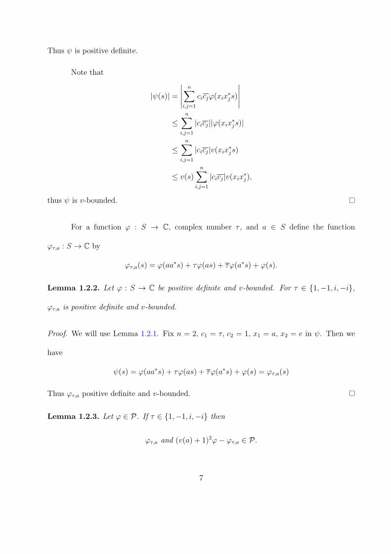
Thus ψ is positive definite.
Note that
|ψ(s)| =
∣∣∣∣∣n∑
i,j=1
cicjφ(xix∗js)
∣∣∣∣∣≤
n∑i,j=1
|cicj||φ(xix∗js)|
≤n∑
i,j=1
|cicj|v(xix∗js)
≤ v(s)n∑
i,j=1
|cicj|v(xix∗j),
thus ψ is v-bounded.
For a function φ : S → C, complex number τ , and a ∈ S define the function
φτ,a : S → C by
φτ,a(s) = φ(aa∗s) + τφ(as) + τφ(a∗s) + φ(s).
Lemma 1.2.2. Let φ : S → C be positive definite and v-bounded. For τ ∈ {1,−1, i,−i},
φτ,a is positive definite and v-bounded.
Proof. We will use Lemma 1.2.1. Fix n = 2, c1 = τ, c2 = 1, x1 = a, x2 = e in ψ. Then we
have
ψ(s) = φ(aa∗s) + τφ(as) + τφ(a∗s) + φ(s) = φτ,a(s)
Thus φτ,a positive definite and v-bounded.
Lemma 1.2.3. Let φ ∈ P. If τ ∈ {1,−1, i,−i} then
φτ,a and (v(a) + 1)2φ− φτ,a ∈ P .
7

Proof. Let φ ∈ P . Suppose that for τ ∈ {1,−1, i,−i}. Note that
(φτ,a)γ(s) =∑t∈S
aγ,tφτ,a(ts)
=∑t∈S
aγ,t(φ(aa∗st) + τφ(ast) + τφ(a∗st) + φ(st))
=∑t∈S
aγ,tφ(aa∗st) +
∑t∈S
aγ,tτφ(ast) +∑t∈S
aγ,tτφ(a∗st) +
∑t∈S
aγ,tφ(st)
= φγ(aa∗s) + τφγ(as) + τφγ(a
∗s) + φγ(s)
= (φγ)τ,a(s).
Therefore by Lemma 1.2.2 (φτ,a)γ are positive definite for all γ ∈ Γ, φτ,a is v-bounded. Thus
φτ,a ∈ P .
Next we consider the function (v(a)+1)2φ−φτ,a for τ ∈ {1,−1, i,−i}. Let {c1, . . . , cn} ⊂
C, {x1, . . . , xn} ⊂ S be arbitrary. By Lemma 1.2.1
ψ(s) =n∑
i,j=1
cicjφ(xix∗js)
is positive definite and v-bounded. Therefore by Lemma 1.1.5
|ψ(s)| ≤ ψ(e)v(s).
We want to show that
n∑i,j=1
cicjφτ,a(xix∗j) ≤
n∑i,j=1
cicj(v(a) + 1)2φ(xix∗j)
Since φτ,a is positive definite, we have
n∑i,j=1
cicjφτ,a(xix∗j)
8

=
∣∣∣∣∣n∑
i,j=1
cicjφτ,a(xix∗j)
∣∣∣∣∣=
∣∣∣∣∣n∑
i,j=1
cicjφ(aa∗xix
∗j) + τ
n∑i,j=1
cicjφ(axix∗j) + τ
n∑i,j=1
cicjφ(a∗xix
∗j) +
n∑i,j=1
cicjφτ,a(xix∗j)
∣∣∣∣∣= |ψ(aa∗) + τψ(a) + τψ(a∗) + ψ(e)|
≤ |ψ(aa∗)|+ |ψ(a)|+ |ψ(a∗)|+ |ψ(e)|
≤ ψ(e)v(aa∗) + ψ(e)v(a) + ψ(e)v(a∗) + ψ(e)v(e)
=n∑
i,j=1
cicj(v(a))2φ(xix
∗j) +
n∑i,j=1
cicj2v(a)φ(xix∗j) +
n∑i,j=1
cicjφ(xix∗j)
=n∑
i,j=1
cicj(v(a) + 1)2φ(xix∗j).
Therefore (v(a) + 1)2φ − φτ,a is positive definite for τ ∈ {1,−1, i,−i}. Similarly
((v(a) + 1)2φ− φτ,a)γ are positive definite for all γ ∈ Γ. Thus v(a) + 1)2φ− φτ,a ∈ P .
Let
M = {ρ ∈ V | ργ(e) ≥ 0, γ ∈ Γ}.
Theorem 1.2.4. Let (S, ·) be a commutative semigroup with involution ∗ and neutral element
e. If φ ∈ P, then there exists a unique positive Radon measure µ on M such that
φ(s) =
∫Mρ(s)dµ(ρ),
for all s ∈ S.
Proof. We will find the integral representation for elements of P in the set
A = {φ ∈ P | φ(e) = 1}.
9

If φ(e) = 1 then find the measure µ that corresponds to 1φ(e)
φ. Then φ corresponds to φ(e)µ.
First we will show that the extreme points of A are in M. Let ρ be an extreme point
of A. Suppose that ρτ,a(e) = 0 and ((v(a) + 1)2ρ− ρτ,a)(e) = 0. Then by Lemma 1.2.3
ρτ,aρτ,a(e)
,(v(a) + 1)2ρ− ρτ,a
((v(a) + 1)2ρ− ρτ,a)(e)∈ A.
Note that
ρ =ρτ,a(e)
(v(a) + 1)2ρτ,aρτ,a(e)
+((v(a) + 1)2ρ− ρτ,a)(e)
(v(a) + 1)2(v(a) + 1)2ρ− ρτ,a
((v(a) + 1)2ρ− ρτ,a)(e).
Since ρ is an extreme point ρ = ρτ,aρτ,a(e)
, that is
ρτ,a(e)ρ = ρτ,a.
Since ρτ,a is v-bounded,
|ρτ,a(s)| ≤ ρτ,a(e)v(s).
If ρτ,a(e) = 0, then ρτ,a = 0. So,
ρτ,a(e)ρ = ρτ,a.
Since (v(a) + 1)2ρ− ρτ,a is v-bounded,
((v(a) + 1)2ρ− ρτ,a)(s) ≤ ((v(a) + 1)2ρ− ρτ,a)(e)v(s).
If ((v(a) + 1)2ρ− ρτ,a)(e) = 0, then ((v(a) + 1)2ρ− ρτ,a)(s) = 0 for all s ∈ S. Therefore,
ρτ,a(e)ρ = (v(a) + 1)2ρ(e)ρ = (v(a) + 1)2ρ = ρτ,a.
10

For all a, s ∈ S,
4ρ(as) =∑
τ∈{1,−1,i,−i}
τρτ,a(s).
Hence,
ρ(as) =1
4
∑τ∈{1,−1,i,−i}
τρτ,a(s)
=1
4
∑τ∈{1,−1,i,−i}
τρτ,a(e)ρ(s)
= ρ(s)1
4
∑τ∈{1,−1,i,−i}
τρτ,a(e)
= ρ(s)ρ(a).
Therefore ρ is a character on S and ρ ∈ M, that is ext(A) ⊂ M.
The other inclustion M ⊂ ext(A) can be shown using Corollary 2.5.12 in [9] on p.
60. Thus ext(A) = M.
By the Krein-Milman theorem A = conv(ext(A)). We will construct a Radon measure
on ext(A). Let φ ∈ A = conv(ext(A)). Then there exists a net (ψα) in conv(extA) such that
φ(s) = limαψα(s) for all s ∈ S.
Since
ψα =nα∑k=1
dαkραk ,
for some dαk ≥ 0,nα∑k=1
dαk = 1, ραk ∈ ext(A) and nα ∈ N,
φ(s) = limα
nα∑k=1
dαkραk (s)
11

Then we have for {c1, . . . , cn} ⊂ C and {s1, . . . , sn} ⊂ S∣∣∣∣∣n∑j=1
cjφ(sj)
∣∣∣∣∣ =∣∣∣∣∣n∑j=1
cj limα
nα∑k=1
dαkραk (sj)
∣∣∣∣∣=
∣∣∣∣∣limαnα∑k=1
dαk
n∑j=1
cjραk (sj)
∣∣∣∣∣≤ lim
α
nα∑k=1
dαk supρ∈ext(A)
∣∣∣∣∣n∑j=1
cjρ(sj)
∣∣∣∣∣= sup
ρ∈ext(A)
∣∣∣∣∣n∑j=1
cjρ(sj)
∣∣∣∣∣ .Define s : ext(A) → C by s(ρ) = ρ(s). Note for s1, s2 ∈ S, s1s2(ρ) = ρ(s1s2) =
ρ(s1)ρ(s2) = s1s2(ρ). Now we will construct a function on the set of functions,
B =
{n∑j=1
cj sj
∣∣∣∣∣ cj ∈ C, sj ∈ S, n ∈ N
}
The set B contains the constant functions and separates points thus by the Stone-Weierstrass
theorem B is dense in continuous functions from ext(A) to C, C(ext(A)). Define
F
(n∑j=1
cj sj
)=
n∑j=1
cjφ(sj).
Note if∑n
j=1 cj sj =∑m
k=1 dksk then from the above inequality∣∣∣∣∣n∑j=1
cjφ(sj)−m∑k=1
dkφ(sk)
∣∣∣∣∣ ≤ supρ∈ext(A)
∣∣∣∣∣n∑j=1
cjρ(sj)−m∑k=1
dkρ(sk)
∣∣∣∣∣ = 0.
Thus F is well defined. We extend F to C(ext(A)). Let f ∈ C(ext(A)), then f = limβ
nβ∑j=1
cβj sβj .
Then we define
F (f) = limβF
(nβ∑j=1
cβj sβj
)
12
= limβ
nβ∑j=1
cβjφ(sβj
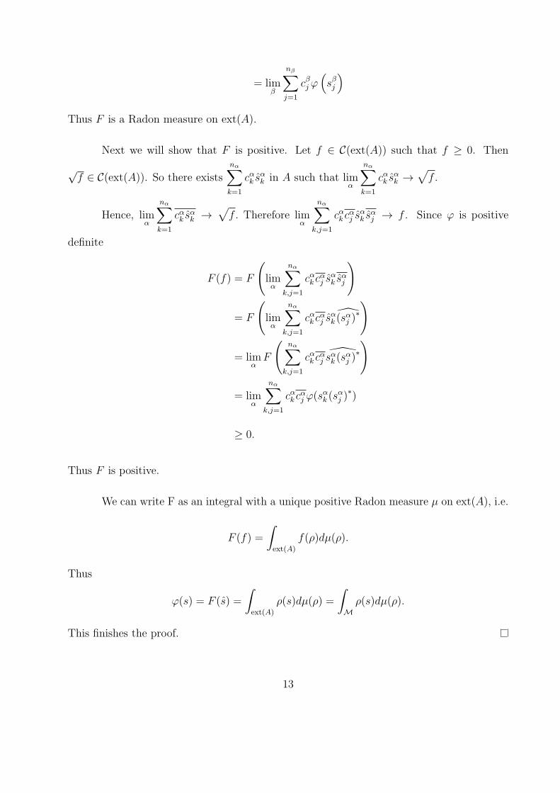
)Thus F is a Radon measure on ext(A).
Next we will show that F is positive. Let f ∈ C(ext(A)) such that f ≥ 0. Then
√f ∈ C(ext(A)). So there exists
nα∑k=1
cαk sαk in A such that lim
α
nα∑k=1
cαk sαk →
√f .
Hence, limα
nα∑k=1
cαk sαk →
√f. Therefore lim
α
nα∑k,j=1
cαk cαj s
αk s
αj → f . Since φ is positive
definite
F (f) = F
(limα
nα∑k,j=1
cαk cαj s
αk s
αj
)
= F
(limα
nα∑k,j=1
cαk cαj s
αk (s
αj )
∗
)
= limαF
(nα∑
k,j=1
cαk cαj s
αk (s
αj )
∗
)
= limα
nα∑k,j=1
cαk cαj φ(s
αk (s
αj )
∗)
≥ 0.
Thus F is positive.
We can write F as an integral with a unique positive Radon measure µ on ext(A), i.e.
F (f) =
∫ext(A)
f(ρ)dµ(ρ).
Thus
φ(s) = F (s) =
∫ext(A)
ρ(s)dµ(ρ) =
∫Mρ(s)dµ(ρ).
This finishes the proof.
13
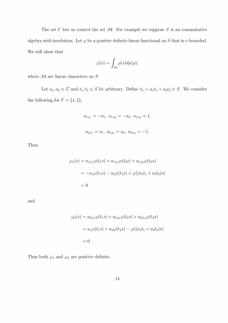
The set Γ lets us control the set M. For example we suppose S is an commutative
algebra with involution. Let φ be a positive definite linear functional on S that is v-bounded.
We will show that
φ(s) =
∫Mρ(s)dµ(ρ),
where M are linear characters on S.
Let a1, a2 ∈ C and t1, t2 ∈ S be arbitrary. Define t3 = a1t1 + a2t2 ∈ S. We consider
the following for Γ = {1, 2},
a1,t1 = −a1, a1,t2 = −a2, a1,t3 = 1,
a2,t1 = a1, a2,t2 = a2, a2,t3 = −1.
Then
φ1(s) = a1,t1φ(t1s) + a1,t2φ(t2s) + a1,t3φ(t3s)
= −a1φ(t1s)− a2φ(t2s) + φ((a1t1 + a2t2)s)
= 0
and
φ2(s) = a2,t1φ(t1s) + a2,t2φ(t2s) + a2,t3φ(t3s)
= a1φ(t1s) + a2φ(t2s)− φ((a1t1 + a2t2)s)
= 0.
Thus both φ1 and φ2 are positive definite.
14

By Theorem 1.2.4
φ(s) =
∫Mρ(s)dµ(ρ),
where M = {ρ ∈ V | ργ(e) ≥ 0, γ ∈ Γ}. That is
a1ρ(t1) + a2ρ(t2) ≤ ρ(a1t1 + a2t2)
and
a1ρ(t1) + a2ρ(t2) ≥ ρ(a1t1 + a2t2).
So
a1ρ(t1) + a2ρ(t2) = ρ(a1t1 + a2t2).
Since a1, a2 and t1, t2 where arbitrary, µ is concentrated on the set of linear characters on S.
Therefore this theory on semigroups can be applied to algebras.
15
CHAPTER 2
SEMIGROUP REPRESENTATIONS
2.1 Introduction
In this chapter H is a Hilbert space and B(H) is the space of bounded operators on H. Let
(S, ·) be a commutative semigroup with an identity e and an involution ∗. We will study
functions of the type U : S → B(H) such that
U(e) = 1, U(s∗) = U(s)∗, U(st) = U(s)U(t),
for all s, t ∈ S. Such a function is called ∗-representation.
This kind of representation was studied in [27] using spectral measures without using
the theory of C∗-algebras or more general Banach algebra arguments. We will use L2 theory
to study this representation instead of spectral measures. We will use the result from Chapter
1 and therefore, as in [27], we will not use Gelfand theory or Banach algebras.
16

2.2 Semigroup Representations
We begin by showing that for a fixed a ∈ H, such that a = 0 the function φa(s) = ⟨U(s)a, a⟩
is positive definitie.
Lemma 2.2.1. The function φa : S → C defined by
φa(s) = ⟨U(s)a, a⟩
is positive definite.
Proof. Let {c1, . . . , cn} ⊂ C, {x1, . . . , xn} ⊂ S be arbitrary. Then
n∑i,j=1
cicjφa(xix∗j) =
n∑i,j=1
cicj⟨U(xix∗j)a, a
⟩=
n∑i,j=1
cicj ⟨U(xi)(U(xj))∗a, a⟩
=n∑
i,j=1
cicj ⟨(U(xj))∗a, (U(xj))∗a⟩
=n∑i=1
n∑j=1
cicj ⟨(U(xj))∗a, (U(xj))∗a⟩
=
⟨n∑i=1
ci(U(xj))∗a,n∑j=1
cj(U(xj))∗a
⟩
=
∥∥∥∥∥n∑i=1
ci(U(xj))∗a
∥∥∥∥∥2
≥ 0.
So, φa is positive definite.
Lemma 2.2.2. The function α(s) = ∥U(s)∥ is an absolute value on S.
17

Proof. Note that the following,
α(e) = ∥U(e)∥ = ∥1H∥ = 1,
α(st) = ∥U(st)∥ = ∥U(s)U(t)∥ ≤ ∥U(s)∥∥U(t)∥,
α(s∗) = ∥U(s∗)∥ = ∥(U(s))∗∥ = ∥U(s)∥ = α(s) for all s, t ∈ S.
Lemma 2.2.3. The function φa is α-bounded.
Proof. Note that
|φa(s)| = | ⟨U(s)a, a⟩ | ≤ ∥U(s)a∥∥a∥ ≤ ∥U(s)∥∥a∥2.
Therefore φa is α-bounded.
Let (aγ,t)γ∈Γ,t∈S be a family of complex numbers such that for every γ in a set Γ there
are finite number of t ∈ S such that aγ,t = 0. We will use Theorem 1.2.4. We will rewrite
the sets V and M from Chapter 1 using the setting of this section.
V = {ρ ∈ S | |ρ(s)| ≤ α(s), s ∈ S} = {ρ ∈ S | |ρ(s)| ≤ ∥U(s)∥, s ∈ S}
and
M = {ρ ∈ V | ργ(e) ≥ 0, γ ∈ Γ}.
Lemma 2.2.4. We suppose (φa)γ are positive definite for all γ ∈ Γ. There exists a positive
Radon measure on M such that
φa(s) =
∫Mρ(s)dµa(ρ),
for all s ∈ S.
18

Proof. By Lemma 2.2.4 φa is positive definite and by Lemma 2.2.3 φa is α-bounded. Also,
by assumption (φa)γ are positive definite for all γ ∈ Γ. Therefore by Theorem 1.2.4 there
exists a unique positive Radon measure, µa, on M such that for all s ∈ S,
φa(s) =
∫Mρ(s)dµa(ρ).
Define
Ka = supp µa.
Lemma 2.2.5. Let {c1, . . . , cn}, {d1, . . . , dm} ⊂ C, {s1, . . . , sn}, {t1, . . . , tm} ⊂ S be arbi-
trary. Then ⟨n∑j=1
cjU(sj)a,m∑k=1
djU(tk)a
⟩=
∫Ka
n∑j=1
cjρ(sj)m∑k=1
dkρ(tk)dµa(ρ).
Proof. Let {c1, . . . , cn}, {d1, . . . , dm} ⊂ C, {s1, . . . , sn}, {t1, . . . , tm} ⊂ S be arbitrary. Then⟨n∑j=1
cjU(sj)a,m∑k=1
djU(tk)a
⟩=
n∑j=1
cj
m∑k=1
dk ⟨U(sj)a,U(tk)a⟩
=n∑j=1
cj
m∑k=1
dk ⟨(U(tk))∗U(sj)a, a⟩
=n∑j=1
cj
m∑k=1
dk ⟨U(t∗ksj)a, a⟩
=n∑j=1
cj
m∑k=1
dk
∫Ka
ρ(sjt∗k)dµa(ρ)
=n∑j=1
cj
m∑k=1
dk
∫Ka
ρ(sj)ρ(tk)dµa(ρ)
19

=
∫Ka
n∑j=1
cjρ(sj)m∑k=1
dkρ(tk)dµa(ρ).
Define s : Ka → C by
s(ρ) = ρ(s).
Lemma 2.2.6. The set{∑n
j=1 cj sj
∣∣∣ cj ∈ C, sj ∈ S, n ∈ N}
is dense in L2(Ka, µa).
Proof. By the Stone-Weierstrass the set of functions∑n
j=1 cj sj is dense in the set on all
continuous on Ka with uniform norm. Since the measure in the compact set Ka is finite the
set of functions∑n
j=1 cj sj are dense in the set on all continuous on Ka with the L2 norm. The
continuous functions are dense in L2 with L2 norm. Thus{∑n
j=1 cj sj
∣∣∣ cj ∈ C, sj ∈ S, n ∈ N}
is dense in L2(Ka, µa).
Define the function
ξa :
{n∑j=1
cjU(sj)a
∣∣∣∣∣ cj ∈ C, sj ∈ S, n ∈ N
}→
{n∑j=1
cj sj
∣∣∣∣∣ cj ∈ C, sj ∈ S, n ∈ N
}by
ξa
(n∑j=1
cjU(sj)a
)=
n∑j=1
cj sj.
Now we will show that ξa is well defined. Suppose that∑n
j=1 cjU(sj)a =∑m
k=1 dkU(tk)a.
Then∥∥∥∥∥n∑j=1
cj sj −m∑k=1
dk tk
∥∥∥∥∥2
L2(Ka,µa)
=
∫Ka
∣∣∣∣∣n∑j=1
cjρ(sj)−m∑k=1
dkρ(tk)
∣∣∣∣∣2
dµa(ρ)
20

=
⟨n∑j=1
cjU(sj)a−m∑k=1
dkU(tk)a,n∑j=1
cjU(sj)a−m∑k=1
dkU(tk)a
⟩
=
∥∥∥∥∥n∑j=1
cjU(sj)a−m∑k=1
dkU(tk)a
∥∥∥∥∥2
H
= 0.
Since Ka is the support of µa,n∑j=1
cj sj =m∑k=1
dk tk
and ξa is well defined. From the definition we note that ξa is linear. Next we will show that
ξa is isometric and thus continuous. By Lemma 2.2.5⟨n∑j=1
cjU(sj)a,n∑j=1
cjU(sk)a
⟩=
∫Ka
∣∣∣∣∣n∑j=1
cjρ(sj)
∣∣∣∣∣2
dµa(ρ).
Thus, ∥∥∥∥∥ξa(
n∑j=1
cjU(sj)a
)∥∥∥∥∥2
L2(Ka,µa)
=
∥∥∥∥∥n∑j=1
cj sj
∥∥∥∥∥2
L2(Ka,µa)
=
∫K
∣∣∣∣∣n∑j=1
cjρ(sj)
∣∣∣∣∣2
dµa(ρ)
=
⟨n∑j=1
cjU(sj)a,n∑j=1
cjU(sk)a
⟩
=
∥∥∥∥∥n∑j=1
cjU(sk)a
∥∥∥∥∥2
H
.
Since ξa is continuous, we can extend ξa to be a map from Ha to L2(K,µa), where
Ha =
{n∑j=1
cjU(sj)a
∣∣∣∣∣ cj ∈ C, sj ∈ S, n ∈ N
}⊂ H.
Theorem 2.2.7. The spaces Ha and L2(Ka, µa) are isomorphic Hilbert spaces.
21

Proof. We will show that ξa is an isomorphism from Ha to L2(Ka, µa)
First we show that ξa is surjective. Let f ∈ L2(Ka, µa). Then there exists a sequence(∑nk
j=1 cj,ksj,k
)∞k=1
such that
f = limk→∞
nk∑j=1
cj,ksj,k.
Therefore,
ξa
(limk→∞
nk∑j=1
cj,kU(sj,k)a
)= lim
k→∞ξa
(nk∑j=1
cj,kU(sj,k)a
)
= limk→∞
nk∑j=1
cj,ksj,k
= f.
Therefore ξa is surjective.
Since ξa is linear, surjective, and⟨n∑j=1
cjU(sj)a,m∑k=1
djU(tk)a
⟩=
∫K
n∑j=1
cjρ(sj)m∑k=1
dkρ(tk)dµa(ρ),
ξa is an isomorphism from Ha to L2(Ka, µa).
Let Mg where g ∈ L∞(Ka) be the multiplication operator on L2(Ka, µa), that is for
f ∈ L2(Ka, µa)
Mgf = gf.
Lemma 2.2.8.
1. Ha is U(s) invariant for all s ∈ S.
22

2. U(s) corresponds to Ms on L2(Ka, µa).
Proof. Proof of 1.
Let h ∈ Ha. Then
h = limk→∞
nk∑j=1
cj,kU(sj,k)a,
for nk ∈ N, cj,k ∈ C and sj,k ∈ S. Then for s ∈ S,
U(s)h = U(s) limk→∞
nk∑j=1
cj,kU(sj,k)a
= limk→∞
nk∑j=1
cj,kU(s)U(sj,k)a
= limk→∞
nk∑j=1
cj,kU(ssj,k)a.
Since limk→∞∑nk
j=1 cj,kU(ssj,k)a ∈ Ha, Ha is U(s) invariant for all s ∈ S.
Proof of 2.
ξa (U(s)h) = ξa
(limk→∞
nk∑j=1
cj,kU(ssj,k)a
)
= limk→∞
nk∑j=1
cj,kssj,k
= s limk→∞
nk∑j=1
cj,ksj,k
= sξa(h)
=Msξa(h).
23

Theorem 2.2.9. If H is separable, then there exist a1, a2, · · · ∈ H such that
H =∞⊕n=1
Han ≃∞⊕n=1
L2(Kan , µan)
Proof. Fix a1 ∈ H. Then we construct Ha1 . If Ha1 = H, then H = Ha1 ≃ L2(Ka1 , µa1).
Suppose that Ha1 = H. Let a2 ∈ H⊥a1, where H⊥
a1is the orthogonal compliment of Ha1 . Then
consider Ha1
⊕Ha2 . If Ha1
⊕Ha2 = H, then let a3 ∈ (Ha1
⊕Ha2)
⊥. Since H is separable,
we continue to find a countable number of an ∈ H such that H =⊕∞
n=1Han . From Theorem
2.2.7 we have
H =∞⊕n=1
Han ≃∞⊕n=1
L2(Kan , µan).
2.3 Examples
Example 2.3.1. Let H be a separable Hilbert space and A a positive operator on H. This
means that we have ⟨Ah, h⟩ ≥ 0.
Let S be the semigroup (N0,+) with involution n∗ = n. Consider U : S → B(H) defined by
U(n) = An
Take a ∈ H. The functions n 7→ ⟨Ana, a⟩ and n 7→ ⟨An+1a, a⟩ are positive definite. This
implies that there is a positive Radon measure µa on K = [0, ∥A∥] such that
⟨Ana, a⟩ =∫K
xndµa(x) =
∫Ka
xndµa(x).
24
where Ka is the support of the measure µa.
This is because a character on N0 is of the form n 7→ xn and can be identified with the real
number x.
We have
Ha =
{n∑j=0
cjAja
∣∣∣∣∣ cj ∈ R, n ∈ N0
}and
H =∞⊕n=1
Han ≃∞⊕n=1
L2(Kan , µan). (2.3.1)
Denote by ξa the isomorphism
Ha → L2(Ka, µa),
we have by Lemma 2.2.8
ξa(Anh) =Mnξa(h), (2.3.2)
where the function n : Ka → R is defined by n(x) = xn.
The equality (2.3.2) is equivalent to
Anh = ξ−1a Mnξa(h), for all h ∈ Ha
We consider the operator M√1on L2(Ka, µa). We have
ξ−1a M√
1ξaξ
−1a M√
1ξa(h) = ξ−1
a M1ξa(h) = Ah, for all h ∈ Ha
Now using (2.3.1) we have proved that a positive operator has a square root.
Example 2.3.2. Let H be a separable Hilbert space and T a normal operator on H. Let S
be the semigroup (N20,+) with involution (m,n)∗ = (n,m). Consider U : S → B(H) defined
25

by
U(m,n) = Tm(T ∗)n.
Fix a ∈ H. We supppose the functions
(m,n) 7→⟨Tm+1(T ∗)na+ Tm(T ∗)n+1a, a
⟩and
(m,n) 7→ 1
i
⟨Tm+1(T ∗)na− Tm(T ∗)n+1a, a
⟩are positive definite. This implies that there is a positive Radon measure µa on
K = {z ∈ C | |z| ≤ ∥T∥,ℜz ≥ 0,ℑz ≥ 0}
such that
⟨Tm(T ∗)na, a⟩ =∫K
znzmdµa(z) =
∫Ka
znzmdµa(z).
where Ka is the support of the measure µa.
This is because a character on (N20,+) is of the form (n,m) 7→ znzm and can be identified
with the complex number z.
Denote by ξa the isomorphism
Ha → L2(Ka, µa).
We have by Lemma 2.2.8
ξa(Tm(T ∗)nh) =M
(m,n)ξa(h) (2.3.3)
where the function (m,n) : Ka → C is defined by (m,n)(z) = znzm.
The equality (2.3.5) is equivalent to
Tm(T ∗)nh = ξ−1a M
(m,n)ξa(h), for all h ∈ Ha
26

This yields
Th = ξ−1a M
(1,0)ξa(h), for all h ∈ Ha
Example 2.3.3. Let H be a separable Hilbert space and A,B and C commuting selfadjoint
operators on H. Let S be the semigroup (N30,+) with involution (m,n, p)∗ = (n,m, p).
Consider U : S → B(H) defined by
U(m,n, p) = AmBnCp
Fix a ∈ H. We supppose the function
(m,n, p) 7→⟨(Am+2BnCp + AmBn+2Cp − AmBnCp+1)a, a
⟩is positive definite.
This implies that there is a positive Radon measure µa on
K ={(x, y, z) ∈ R3 | |x| ≤ ∥A∥, |y| ≤ ∥B∥, |z| ≤ ∥C∥, x2 + y2 − z ≥ 0
}such that
⟨AmBnCpa, a⟩ =∫K
xnynzpdµa(x, y, z) =
∫Ka
xnynzpdµa(x, y, z).
where Ka is the support of the measure µa.
This is because a character on (N30,+) is of the form (n,m, p) 7→ xnynzp and can be identified
with the element (x, y, z) ∈ R3.
Denote by ξa the isomorphism
Ha → L2(Ka, µa).
27

We have by Lemma 2.2.8
ξa(AmBnCph) =M (m,n,p)ξa(h) (2.3.4)
where the function (m,n, p) : Ka → R is defined by (m,n, p)(x, y, z) = xnynzp.
Example 2.3.4. Let H be a separable Hilbert space . Let S be a commutative normed
algebra with involution and unity e. Consider a linear ∗-representation U : S → B(H).
Fix a ∈ H. We supppose the functions
s 7→⟨(∥t∥2U(s)− U(tt∗s))a, a
⟩are positive definite for every t.
This implies that there is a positive Radon measure µa on
K = {ρ : S → C | ρ(e) = 1, ρ linear , ρ(s∗) = ρ(s), |ρ(s)| ≤ ∥t∥, ρ(st) = ρ(s)ρ(t), s, t ∈ S}.
such that
⟨U(s)a, a⟩ =∫K
ρ(s)dµa(ρ) =
∫Ka
ρ(s)dµa(z),
where Ka is the support of the measure µa.
Denote by ξa the isomorphism
Ha → L2(Ka, µa),
we have by Lemma 2.2.8
ξaU(s)h =Msξa(h) (2.3.5)
28

where the function s : Ka → C is defined by s(ρ) = ρ(s).
The equality (2.3.5) is equivalent to
U(s)h = ξ−1a Msξa(h), h ∈ Ha.
29

CHAPTER 3
INTEGRATED CAUCHY FUNCTIONAL EQUATION ON
COMMUTATIVE SEMIGROUPS
3.1 Introduction
In this chapter we are considering an expansion of a theorem by Ressel which will be intro-
duced later. The original idea of this theorem comes from a theorem by DeFinetti about
probability measures.
Theorem 3.1.1. [DeFinetti 1931] Let X1, X2, . . . be {0, 1} valued random variables such
that
P (X1 = x1, . . . , Xn = xn) = P (X1 = xσ(1), . . . , Xn = xσ(n))
(exchangeable sequence) for all n ∈ N, x1, . . . , xn ∈ {0, 1} and all permutations σ of {1, . . . , n}.
Then for some unique probability measure µ on [0, 1] we have
P (X1 = x1, . . . , Xn = xn) =
∫[0,1]
p∑n
i=1 xi(1− p)n−∑n
i=1 xidµ(p).
30

We now look at this from a different angle by considering the following function.
Define the function φ : N20 → [0, 1] by
φ
(n∑i=1
xi, n−n∑i=1
xi
)= P (X1 = x1, . . . , Xn = xn),
for all n ∈ N, x1, . . . , xn ∈ {0, 1}. We will show that φ is well defined on N20. For (s, t) ∈ N2
0,
we use (s, t) = (s, (t+ s)− s). Therefore n = t+ s and∑n
i=1 xi = s. So
φ(s, t) = P (X1 = 1, . . . , Xs = 1, Xs+1 = 0, . . . , Xs+t = 0),
which is well defined since X1, X2, . . . is an exchangeable sequence. Also,
φ(s, t) ≥ 0
because P is a probability. Note that
φ(0, 0) = 1
and
φ(s+ 1, t) + φ(s, t+ 1) = P (X1 = 1, . . . , Xs = 1, Xs+1 = 0, . . . , Xs+t = 0, Xs+t+1 = 1)
+ P (X1 = 1, . . . , Xs = 1, Xs+1 = 0, . . . , Xs+t = 0, Xs+t+1 = 0)
= P (X1 = 1, . . . , Xs = 1, Xs+1 = 0, . . . , Xs+t = 0)
= φ(s, t).
This leads to the following generalization about functional equations on semigroups.
31

Theorem 3.1.2 (Cauchy functional equation on the semigroup (N20,+)). For a function
φ : N20 → [0,∞) the following conditions are equivalent:
1. The function, φ, satisfies
φ(0, 0) = 1
and
φ(s+ 1, t) + φ(s, t+ 1) = φ(s, t).
2. There is a unique probability measure µ on [0, 1] such that
φ(l,m) =
∫[0,1]
pl(1− p)mdµ(p).
Theorem 3.1.2 is a consequence of Theorem 3.2.1 which was proven by Ressel in [25]
(see also [26]).
For the rest of this chapter we need a few preliminary ideas.
3.2 Defintions and Preliminary Concepts
We consider a commutative semigroup (S,+) with neutral element 0. A set G ⊂ S is a
generator set for S if every element s ∈ S \ {0} is a finite sum of elements from G.
Recall that a function ρ : S → R is a character of S if it satisfies ρ(0) = 1 and
ρ(s+ t) = ρ(s)ρ(t), s, t ∈ S.
32

Let S be the set of characters on the semigroup S. The topology on S is the topology
of pointwise convergence which is locally convex.
We will generalize the following result, from [25], to a system of equations.
Theorem 3.2.1. Let S be a commutative semigroup, with a countable generator set G ⊂ S
and let β : G→ (0,∞) be a function.
A function φ : S → [0,∞) is a solution of the equation
φ(s) =∑a∈G
β(a)φ(a+ s)
if and only if there exists a positive Radon measure µ concentrated on K such that
φ(s) =
∫K
ρ(s)dµ(ρ),
where K =
{ρ ∈ S
∣∣∣∣∣ ρ(s) ≥ 0,∑a∈G
β(a)ρ(a) = 1
}.
Recall a function φ : S → R is called positive definite if
n∑j,k=1
cjckφ(sj + sk) ≥ 0,
for all n ∈ N, {s1, . . . , sn} ⊂ S, {c1, . . . , cn} ⊂ R.
Define the operator Es that maps the set of functionals from S to R to itself by,
Es(φ)(t) = φ(t+ s)
where φ : S → R. The operators (Es)s∈S generate an algebra.
33

3.3 System of Cauchy Functional Equations
Theorem 3.3.1. Let S be a countable commutative semigroup, G ⊂ S be a generator set
and let {βi : G→ [0,∞)}i∈I be a family of functions where I is an indexing set. We suppose
that for every a ∈ G there is an i ∈ I such that βi(a) > 0.
A function φ : S → [0,∞) is a solution of the system
φ(s) =∑a∈G
βi(a)φ(a+ s), i ∈ I
if and only if there exists a positive Radon measure µ concentrated on K such that
φ(s) =
∫K
ρ(s)dµ(ρ),
where K =
{ρ ∈ S
∣∣∣∣∣ ρ(s) ≥ 0,∑a∈G
βi(a)ρ(a) = 1, i ∈ I
}. That is, solutions to the system
can be identified with positive Radon measures concentrated on K.
Proof. First we will state an inequality that will be used throughout the proof. Suppose φ
is a solution to the system of functional equations, φ(s) =∑
a∈G βi(a)φ(a+ s), i ∈ I. Then,
for s ∈ S, a ∈ G and i ∈ I,
φ(s) ≥ βi(a)φ(s+ a).
Fix s ∈ S, then s =n∑k=1
ak for ak ∈ G and n ∈ N. Therefore, for every ak there exists a βik
such that βik(ak) > 0. Hence,
φ(s) = φ
(n∑k=1
ak
)
34
= φ
(n−1∑k=1
ak + an
)
≤ (βin(an))−1φ
(n−1∑k=1
ak
)...
≤n∏k=1
(βik(ak))−1φ(0).
Therefore, for every s ∈ S there exists γs such that
φ(s) ≤ γsφ(0), (3.3.1)
where γs =∏n
k=1(βik(ak))−1. Therefore, if φ(0) = 0 then φ ≡ 0. The zero function is
identified with the zero measure on K. If φ(0) = c > 0, then we will find the representation
of 1cφ then multiply the measure by c. So, without loss of generality we will consider functions
φ such that φ(0) = 1. That is the set,
P =
{φ : S → [0,∞)
∣∣∣∣∣ φ(0) = 1, φ(s) =∑a∈G
βi(a)φ(s+ a), i ∈ I
}.
However, P is not necessarily closed and therefore not necessarily compact. We would like
to use the Krein-Milman theorem thus we will find a compact convex set that contains P .
Consider
P1 =
{φ : S → [0,∞)
∣∣∣∣∣ ∏a∈F
(E0 − βia(a)Ea)φ(s) ≥ 0, F ⊂ G,F finite, {ia} ⊂ I, φ(0) = 1
}.
We will show that P1 is convex. Let φ, ψ ∈ P1 and λ ∈ (0, 1). We will show that
λφ+ (1− λ)ψ ∈ P1. Note λφ(0) + (1− λ)ψ(0) = λ+ (1− λ) = 1. Let F ⊂ G such that F
35

is finite and {ia} ⊂ I. Then
∏a∈F
(E0 − βia(a)Ea)(λφ(s) + (1− λ)ψ(s))
= λ∏a∈F
(E0 − βia(a)Ea)φ(s) + (1− λ)∏a∈F
(E0 − βia(a)Ea)ψ(s) ≥ 0.
Hence, P1 is convex.
Note that P1 is closed in the topology of pointwise convergence. We will show that
P1 is a subset of a compact set. First consider F to be the singleton {a} and φ ∈ P1. Then
the condition of P1 is (E0 − βia(a)Ea)φ(s) ≥ 0, i.e. φ(s) ≥ βi(a)φ(s + a). Thus, inequality
(3.3.1) holds for φ ∈ P1. Since φ ∈ P1, inequality (3.3.1) simplifies to
φ(s) ≤ γs.
Thus P1 is a closed subset of∏s∈S
[0, γs]. By Tychonoff theorem∏s∈S
[0, γs] is compact.
Hence P1 is compact. So P1 is a compact convex set and by Krein-Milman theorem, P1 =
conv(ext(P1)).
We will show that P ⊂ P1. Let φ ∈ P , F ⊂ G such that F is finite, and {ia} ⊂ I.
Then
(E0 − βi1(b1)Eb1)φ(s) =∑a∈Ga =b1
βi1(a)φ(s+ a) ≥ 0
and
(E0−βi2(b2)Eb2)(E0−βi1(b1)Eb1)φ(s) =∑a(1)∈Ga(1) =b1
βi1(a(1)) ∑a(2)∈Ga(2) =b2
βi2(a(2))φ(s+a(1)+a(2)) ≥ 0.
36

Continuing this process we get
n∏k=1
(E0 − βik(bk)Ebk)φ(s)
=∑a(1)∈Ga(1) =b1
βi1(a(1)) ∑a(2)∈Ga(2) =b2
βi2(a(2))· · ·
∑a(n)∈Ga(n) =bn
βin(a(n))φ
(s+
n−1∑k=1
a(k)
)
≥ 0.
Thus P ⊂ P1.
Let φ ∈ ext(P1). We will now show that φ is a character. Case 1, suppose b ∈ G
such that φ(b) > 0, βi(b) > 0 and 1− βi(b)φ(b) > 0.
Define
ψ1(s) = φ(s+ b) and ψ2(s) = φ(s)− βi(b)φ(s+ b).
Note thatψ1
φ(b),
ψ2
1− βi(b)φ(b)∈ P and
φ(s) = βi(b)φ(b)ψ1(s)
φ(b)+ (1− βi(b)φ(b))
ψ2(s)
1− βi(b)φ(b).
Since φ is extreme, this implies φ(s) =ψ1(s)
φ(b), i.e.
φ(s+ b) = φ(s)φ(b).
For the last 2 cases we will use the following. If ψ satisfies
∏a∈F
(E0 − βi(a)Ea)ψ(s) ≥ 0, F ⊂ G,F finite, i ∈ I (3.3.2)
37

then for all s ∈ S there exists γs > 0 such that γsψ(0) ≥ ψ(s). Note ψ1 and ψ2 satisfy
condition (3.3.2).
Case 2, suppose b ∈ G such that φ(b) = 0. Then 0 ≤ φ(s + b) = ψ1(s) ≤ γsψ1(0) =
γsφ(b) = 0. Thus φ(s+ b) = 0 = φ(s)φ(b).
Case 3, suppose b ∈ G such that 1 − βi(b)φ(b) = 0. Then φ(b) = (βi(b))−1. Thus
φ(s) − βi(b)φ(s + b) = ψ2(s) ≤ γsψ2(0) = γs(1 − βi(b)φ(b)) = 0. Hence φ(s + b) =
φ(s)(βi(b))−1 = φ(s)φ(b).
Therefore, for all a ∈ G and s ∈ S, φ(s+ a) = φ(s)φ(a). This implies for all s, t ∈ S,
φ(s+ t) = φ(s)φ(t). Thus extP1 ⊂ S ∩ P1.
We will construct a Radon measure on ext(P1) as in Chapter 1 which is inspired
by [19]. Let φ ∈ P1 = conv(extP1). Then there exists a net (ψα) in conv(ext(P1)) such that
φ(s) = limαψα(s) for all s ∈ S.
Since
ψα =nα∑k=1
dαkραk ,
for some dαk ≥ 0,nα∑k=1
dαk = 1, ραk ∈ ext(P1) and nα ∈ N,
φ(s) = limα
nα∑k=1
dαkραk (s).
Then we have for {c1, . . . , cn} ⊂ R and {s1, . . . , sn} ⊂ S∣∣∣∣∣n∑j=1
cjφ(sj)
∣∣∣∣∣ =∣∣∣∣∣n∑j=1
cj limα
nα∑k=1
dαkραk (sj)
∣∣∣∣∣
38

=
∣∣∣∣∣limαnα∑k=1
dαk
n∑j=1
cjραk (sj)
∣∣∣∣∣≤ lim
α
nα∑k=1
dαk supρ∈ext(P1)
∣∣∣∣∣n∑j=1
cjρ(sj)
∣∣∣∣∣= sup
ρ∈ext(P1)
∣∣∣∣∣n∑j=1
cjρ(sj)
∣∣∣∣∣ .Define s : ext(P1) → [0,∞) by s(ρ) = ρ(s). Note for s1, s2 ∈ S, s1 + s2(ρ) = ρ(s1 +
s2) = ρ(s1)ρ(s2) = s1s2(ρ). Now we will construct a function on the set of functions,
A =
{n∑j=1
cj sj
∣∣∣∣∣ cj ∈ R, sj ∈ S, n ∈ N
}.
The set A contains the constant functions and separates points thus, by the Stone-Weierstrass
theorem, A is dense in continuous functions from ext(P1) to R, C(ext(P1)). Define
F
(n∑j=1
cj sj
)=
n∑j=1
cjφ(sj).
Note if∑n
j=1 cj sj =∑m
k=1 dksk then from the above inequality∣∣∣∣∣n∑j=1
cjφ(sj)−m∑k=1
dkφ(sk)
∣∣∣∣∣ ≤ supρ∈ext(P1)
∣∣∣∣∣n∑j=1
cjρ(sj)−m∑k=1
dkρ(sk)
∣∣∣∣∣ = 0.
Thus F is well defined. We extend F to C(ext(P1)). Let f ∈ C(ext(P1)), then f =
limβ
nβ∑j=1
cβj sβj . Then we define
F (f) = limβF
(nβ∑j=1
cβj sβj
)
= limβ
nβ∑j=1
cβjφ(sβj
).
39

Thus F is a Radon measure on ext(P1).
Next we will show that F is positive. Let f ∈ C(ext(P1)) such that f ≥ 0. Then
√f ∈ C(ext(P1)). So there exists
nα∑k=1
cαk sαk in A such that lim
α
nα∑k=1
cαk sαk →
√f. Therefore
limα
nα∑k,j=1
cαk cαj s
αk s
αj → f . So it suffices to show that
F
(nα∑
k,j=1
cαk cαj s
αk s
αj
)= F
(nα∑
k,j=1
cαk cαj ( sαk + sαj )
)
=nα∑
k,j=1
cαk cαj φ(s
αk + sαj )
≥ 0,
for all cαk ∈ R and sαk ∈ S. We will show φ is positive definite using the same method as
in [3], which simplifies the method used in [20]. Let {c1, . . . , cn} ⊂ R and {s1, . . . , sn} ⊂ S.
Thenn∑
k,j=1
ckcjφ(sk + sj) =
(n∑k=1
ckEsk
)2
φ(0). We will split the sum into the parts where
ck are positive and ck are negative(n∑k=1
ckEsk
)2
=
(∑ck>0
ckEsk −∑ck<0
(−ck)Esk
)2
.
Let X =∑ck>0
ckEsk and Y =∑ck<0
(−ck)Esk . It suffices to show that
(X − Y )2φ(0) ≥ 0.
Note that for s, t ∈ S, where t =∑m
j=1 aj, aj ∈ G and βij(aj) > 0,
φ(s+ t) = φ
(s+
m∑j=1
aj
)
= φ
(s+
n−1∑j=1
aj + am
)
40
≤ (βim(am))−1φ
(s+
m−1∑j=1
aj
)...
≤m∏j=1
(βij(aj))−1φ(s).
Let γt =m∏j=1
(βij(aj))−1. Then we have φ(s+ t) ≤ γtφ(s). Thus
Xφ(s) =
(∑ck>0
ckEsk
)φ(s)
=∑ck>0
ckφ (s+ sk)
≤ nmaxck>0
{ckγsk}φ(s).
Hence for M = nmaxck>0
{ckγsk} > 0, U = ME0 − X ≥ 0. Similarly there exists Q > 0 such
that V = QE0 − Y ≥ 0.
We will show that U and V are greater that or equal to a finite sum with positive
coefficients of products of the form
m1∏k=1
dkEak
m2∏j=1
(E0 − βij(aj)Eaj). (3.3.3)
First suppose X = cEt then M = cγt. So
ME0 −X = cγtE0 − cEt
= cγt(E0 − γ−1t Et)
41
= cγt
(E0 −
m∏j=1
βij(aj)Eaj
)
= cγt
(E0 − βi1Ea1(E0 − βi2Ea2) + · · ·+
m−1∏j=1
(βij(aj)Eaj)(E0 − βim(am)Eam)
).
Next suppose X =∑n
k=1Etk then M = nmax γtk . Then
ME0 −X = nmax{γtk} −n∑k=1
Etk
≥n∑k=1
γtkE0 −n∑k=1
Etk
=n∑k=1
(γtkE0 − Etk).
From above each γtkE0 − Etk can be bounded below by a sum of products of the form
(3.3.3). From the combination of these two cases we have that U has the desired lower
bound. Similarly we can show that V has the same type of lower bound. Since φ ∈ P1,
we have that products of U, V,X, Y are bounded bellow by product of the form (3.3.3) and
therefore are nonnegative. Let
C(n, j, k) =
(n
j
)(n
k
)XjUn−jY kV n−k.
Now consider the following for n ≥ 2.
Zn =n∑
j,k=1
[j2M2 + k2Q2
n(n− 1)− 2
jkMQ
n2
]C(n, j, k)
Note that Zn ≥ 0 and
Zn =n∑
j,k=1
[j(j − 1)M2
n(n− 1)+k(k − 1)Q2
n(n− 1)− 2
jM
n
kQ
n+
jM2
n(n− 1)+
kQ2
n(n− 1)
]C(n, j, k)
42

= (X − Y )2MnQn +X
n− 1Mn+1Qn +
Y
n− 1MnQn+1.
Therefore (X − Y )2φ(0) + XMn−1
φ(0) + Y Qn−1
φ(0) ≥ 0, for all n ≥ 2. Hence (X − Y )2φ(0) ≥ 0.
Thus φ is positive definite and F is positive.
We can write F as an integral with a unique positive Radon measure µ on ext(P1),
i.e.
F (f) =
∫ext(P1)
f(ρ)dµ(ρ).
Thus
φ(s) = F (s) =
∫ext(P1)
ρ(s)dµ(ρ).
Now consider φ ∈ P . Then for each i ∈ I we have
∫ext(P1)
ρ(s)dµ(ρ) = φ(s)
=∑a∈G
βi(a)φ(a+ s)
=
∫ext(P1)
∑a∈G
βi(a)ρ(a+ s)dµ(ρ)
=
∫ext(P1)
ρ(s)∑a∈G
βi(a)ρ(a)dµ(ρ).
Thus for φ ∈ P , µ is concentrated on the set
K =
{ρ ∈ S
∣∣∣∣∣ ρ(s) ≥ 0,∑a∈G
βi(a)ρ(a) = 1, i ∈ I
}.
43
3.4 Examples
The following are some examples that use Theorem 3.3.1.
Example 3.4.1. We consider the semigroup (N30,+) and the system of Cauchy functional
equations
φ(m,n, p) = φ(m+ 1, n, p) + φ(m,n, p+ 1)
φ(m,n, p) = φ(m,n+ 1, p) + φ(m,n, p+ 1)
where φ : N30 → [0,∞).
By Theorem 3.3.1 solutions of this system are
φ(m,n, p) =
∫K
ρ(m,n, p)dµ(ρ),
where K ={ρ ∈ N3
0
∣∣∣ ρ ≥ 0, ρ(1, 0, 0) + ρ(0, 0, 1) = 1, ρ(0, 1, 0) + ρ(0, 0, 1) = 1}
and µ is a
positive Radon measure. That is, solutions of the system can be identified with positive
Radon Measures on K.
To simplify K, we consider what it means to be a character on N30. If ρ is a character
on N30, then
ρ(m,n, q) = ρ((m, 0, 0) + (0, n, 0) + (0, 0, q)
= ρ(m, 0, 0)ρ(0, n, 0)ρ(0, 0, q)
= ρ(m(1, 0, 0))ρ(n(0, 1, 0))ρ(q(0, 0, 1))
= [ρ(1, 0, 0)]m[ρ(0, 1, 0)]n[ρ(0, 0, 1)]q.
44

So, ρ is determined entirely by its values on (1, 0, 0), (0, 1, 0), and (0, 0, 1). Thus for every
character ρ on N30 there exists x, y, z ∈ R such that
ρ(m,n, q) = xmynzq.
The conditions ρ(1, 0, 0)+ρ(0, 0, 1) = 1, ρ(0, 1, 0)+ρ(0, 0, 1) = 1, and ρ ≥ 0 become x+z = 1,
y + z = 1, and x, y, z,∈ R+, respectively.
Thus the solutions of this system are
φ(m,n, p) =
∫K
xmynzpdµ(x, y, z).
Where K is the set {(x, y, z) ∈ R3
+
∣∣ x+ z = 1, y + z = 1}
and µ is a positive Radon measure.
Example 3.4.2. We consider the semigroup (N20,+) and the equation
φ(m, q) =n∑k=0
(n
k
)φ((m+ n− k, q + k)) (3.4.1)
where φ : N20 → [0,∞).
Consider the semigroup, S, generated by
{(n, 0), (n− 1, 1), (n− 2, 2), . . . , (0, n)} ⊂ N20.
The equation (3.4.1) can be rewritten as
φ(m, q) =n∑k=0
(n
k
)φ((n− k, k) + (m, q)).
45

Thus by Theorem 3.3.1 the solutions are
φ(m, q) =
∫K
ρ(m, q)dµ(ρ)
where µ is a positive Radon measure, (m, q) ∈ S,K ={ρ ∈ S
∣∣∣ ρ ≥ 0,∑n
k=0
(nk
)ρ(n− k, k) = 1
}.
Let ρ ∈ K. We will show that ρ is completely determined by it’s values on (n, 0) and
(0, n). First we consider ρ on an element of the generator set, then
[ρ(n− k, k)]n = ρ(n(n− k), nk)
= [ρ(n, 0)]n−k[ρ(0, n)]k.
Hence,
ρ(n− k, k) =[(ρ(n, 0))1/n
]n−k [(ρ(0, n))1/n
]k.
Note that,
1 =n∑k=0
(n
k
)ρ(n− k, k)
=n∑k=0
(n
k
)[(ρ(n, 0))1/n
]n−k [(ρ(0, n))1/n
]k=[(ρ(n, 0))1/n + (ρ(0, n))1/n
]n.
Therefore, (ρ(n, 0))1/n + (ρ(0, n))1/n = 1. Let p = (ρ(n, 0))1/n, thus (1 − p) = (ρ(0, n))1/n
and
ρ(n− k, k) = pn−k(1− p)k,
where p ∈ [0, 1].
For (m, q) ∈ S, (m, q) =∑ℓ
i=1(n− ki, ki). Thus m =∑ℓ
i=1(n− ki) and q =∑ℓ
i=1 ki.
46
Hence,
ρ(m, q) = ρ
(nℓ−
ℓ∑i=1
(n− ki),ℓ∑i=1
ki
)
=ℓ∏i=1
ρ((n− ki), ki))
=ℓ∏i=1
pn−ki(1− p)ki
= pm(1− p)q.
So, ρ can be identified with p and therefore identifyK with [0, 1]. Hence for (m, q) ∈ S
we have
φ(m, q) =
∫K
ρ(m, q)dµ(ρ)
=
∫[0,1]
pm(1− p)qdµ(p).
We extend this representation to all of N20 to get for (m, q) ∈ N2
0
φ(m, q) =
∫[0,1]
pm(1− p)qdµ(p).
47

CHAPTER 4
BOCHNER-PLANCHEREL THEOREMS IN ALGEBRAS
WITH INVOLUTION
4.1 Definitions and notation
Let A be an commutative algebra with involution ∗. We will state some definitions for
algebras that are similar to some of the definitions on semigroups.
Definition 4.1.1. An involution on an algebra is a map x 7→ x∗ from A to A such that the
following hold for all x, y ∈ A and λ ∈ C,
(x+ y)∗ = x∗ + y∗, (λx)∗ = λx∗, (xy)∗ = y∗x∗, (x∗)∗ = x.
Definition 4.1.2. A linear functional f : A → C is called positive, if
f(xx∗) ≥ 0, for all x ∈ A.
Definition 4.1.3. A seminorm p is calledmultiplicative if p(x∗) = p(x) and p(xy) ≤ p(x)p(y)
for all x, y ∈ A.
48

Definition 4.1.4. A net (ei)i∈I is a p-bounded approximate identity if p(ei) ≤ 1, i ∈ I and
limi∈I p(x−xei) = 0 for every x ∈ A. If the topology of A is defined by a family of seminorms
{pk}, then (ei) is bounded approximate identity provided (ei) is pk-bounded for every k.
Definition 4.1.5. A multiplicative functional on A is a nonzero homomorphism from A to
C.
The set of nonzero multiplicative functions will be denoted A and is called the set of
characters of A. We have
A = {ρ : A → C | ρ linear, ρ ≡ 0, ρ(xy) = ρ(x)ρ(y), x, y ∈ A}.
If x ∈ A, we define the function x on A by
x(φ) = φ(x).
The map x 7→ x from A to A is called the Gelfand transform on A. Let
Γ(A) = {x | x ∈ A}.
In this chapter we denote the set
K = {ρ ∈ A | ρ(x∗) = ρ(x), |ρ(x)| ≤ p(x)},
where p is a multiplicative seminorm.
The set K is a locally compact space with pointwise topology. Let (ρi) be a net in
K such that ρi → ρ. Note that ρ could be identical to zero, thus ρ is not necessarily in K.
49
Therefore the set K is not necessarily closed. However, if A has a unity e and the seminorm
p satisfies p(e) = 1, then ρ(e) = 1 for all ρ ∈ K. Thus K is a closed subset of the compact
set∏
x∈A[−p(x), p(x)] and therefore compact.
Definition 4.1.6. We say that a function g : A → C admits a Bochner representation if
there exits a positive Radon measure µ on K such that the functions Γ(A) are µ integrable
and we have
g(x) =
∫K
ρ(x)dµ(ρ), x ∈ A.
Note that every function which admits a Bochner representation is linear.
We denote by B the linear subspace of A generated by the products xy, such that
x, y ∈ A.
Definition 4.1.7. We say that a linear function g : B → C admits a Plancherel represen-
tation, if there exits a positive Radon measure µ on K such that the functions Γ(A) are in
L2(K) and we have
g(xy) =
∫K
ρ(xy)dµ(ρ), x, y ∈ A.
Lemma 4.1.8. If g : A → C admits a Plancherel representation then g is positive.
Proof. Assume that g admits a Plancherel representation. Then there exist a positive Radon
measure µ on K such that for all x, y ∈ A,
g(xy) =
∫K
ρ(xy)dµ(ρ).
50
Therefore,
g(xx∗) =
∫K
ρ(xx∗)dµ(ρ)
=
∫K
ρ(x)ρ(x∗)dµ(ρ)
=
∫K
|ρ(x)|2dµ(ρ)
≥ 0.
So g is positive.
We note that a Bochner representation is a Plancherel representation. Thus a function
that admits a Bochner representation is positive.
4.2 Bochner-type integral representations
In this section we will show an alternative proof of Theorem 2.1 in [14], p. 42 (see also [15],
p. 344), which is stated as Theorem 4.2.8. In [14] Γ-Lumer systems (see [18]) were used to
prove this theorem.
Theorem 4.2.1. Let A be an commutative algebra with involution ∗ and unity e. Let p be a
multiplicative seminorm on A such that p(e) = 1. A function g : A → C admits a Bochner
representation if and only if the following conditions are satisfied,
(a) g is a positive linear function
51

(b) |g(x)| ≤ Cp(x) where C is a positive real number not depending on x.
Proof. This theorem is Theorem 4.2.5 in [9], where we consider our algebra as semigroup
with the multiplication operation.
We will now extend Theorem 4.2.1 to an algebra without unity. But in doing so we
will need to add an extra condition to the function g. In Theorem 4.2.6 we will add an extra
condition on to the algebra A instead of the function g.
Let A be an algebra without unity. We will embed A into an algebra with unity
Ae. Let Ae denote the set of all pairs (x, λ), x ∈ A, λ ∈ C. Then Ae is an algebra with
operators.
(x, λ) + (y, µ) = (x+ y, λ+ µ), µ(x, λ) = (µx, µλ)
and
(x, λ)(y, µ) = (xy + λy + µx, λµ)
for x, y ∈ A and λ, µ ∈ C. The identity element for Ae is e = (0, 1) ∈ Ae. As A is
commutative so is Ae. The mapping x 7→ (x, 0) is an algebra isomorphism of A onto an
ideal of codimension one in Ae. Since (x, λ) = (x, 0) + λ(0, 1), it is customary to write the
elements (x, λ) as x + λe. We call Ae the unitization of A. If A has an involution, the
involution on A can be extend to an involution on Ae by (x+ λe)∗ = x∗ + λe.
The following lemma is Proposition 21.7 in [12] on p. 59,
52

Lemma 4.2.2. Let A be an algebra with involution and Ae the unitization of A. Let g be a
positive functional on A. Then g can be extended to a positive functional on Ae if and only
if:
• g(x∗) = g(x)
• There is a finite k ≥ 0 such that |g(x)|2 ≤ kg(xx∗) for all x ∈ A.
An extension denoted ge is defined by ge(x+ λe) = g(x) + kλ.
Let A be and algebra without unity and p be a multiplicative seminorm on A. Let
K denote the set of linear functions ρ : A → C such that the following hold
(a) ρ ≡ 0
(b) ρ(xy) = ρ(x)ρ(y)
(c) ρ(x∗) = ρ(x)
(d) |ρ(x)| ≤ pe(x).
Let Ae be the unitization of A. We extend the seminorm p to a seminorm on Ae by
pe(x+ λe) = p(x) + |λ|.
Let Ke denote the set of linear functions ρ : Ae → C such that the following hold
(a) ρ(e) = 1
53
(b) ρ((x+ λe)(y + γe)) = ρ(x+ λe)ρ(y + γe)
(c) ρ((x+ λe)∗) = ρ((x+ λe))
(d) |ρ((x+ λe))| ≤ p((x+ λe)).
Lemma 4.2.3. The set Ke can be identified with K ∪ {θ} where θ is the function identical
to 0 on A.
Proof. Let η ∈ K. Therefore |η(x)|2 = |η(xx∗)| ≤ p(xx∗). Thus by Lemma 4.2.2, η can be
extended to Ae by ηe(x + λe) = η(x) + λ. It is easily shown that ηe ∈ Ke. Thus K can be
identified with a subset of Ke.
Let ρ ∈ Ke, then ρ(x + λe) = ρ(x) + λρ(e) = ρ(x) + λ. First we suppose that ρ is
identical to 0 on A. Then ρ(x + λe) = ρ(x) + λ = λ. Thus there is exactly one function in
Ke identical to 0 on A. Denote that function by θ, that is θ(x+ λe) = λ.
Now suppose ρ is not identical to 0 on A. Then ρ|A ∈ K. Also,
(ρ|A)e (x+ λe) = ρ|A(x) + λ = ρ(x+ λe).
Thus, Ke can be identified with K ∪ {θ}.
Theorem 4.2.4. Let A be a commutative algebra with involution ∗ and without unity. A
function g : A → C admits a Bochner representation if and only if the following conditions
are satisfied,
54
(a) g is a positive linear function
(b) |g(x)| ≤ Cp(x) for every x ∈ A where C is a positive real number not depending on x
(c) |g(x)|2 ≤Mg(xx∗) for every x ∈ A where M is a positive real number not depending on
x.
Proof. We are going to use Theorem 4.2.1 in this proof. By Lemma 4.2.2 the function g can
be extended to linear positive functional ge on Ae by
ge(x+ λe) = g(x) +Mλ.
We also define
pe(x+ λe) = p(x) + |λ|.
It is easy to verify that pe is a multiplicative seminorm on Ae.
We have
|ge(x+ λe)| ≤ |g(x)|+ |λ|M ≤ max{C,M}pe(x+ λe).
Let Ke denote the set of linear functions ρ : Ae → C such that the following hold
(a) ρ(e) = 1
(b) ρ((x+ λe)(y + γe)) = ρ(x+ λe)ρ(y + γe)
(c) ρ((x+ λe)∗) = ρ((x+ λe))
(d) |ρ((x+ λe))| ≤ pe((x+ λe)).
55

By Theorem 4.2.1, there is a Radon measure ν on Ke such that for every x + λe ∈ Ae we
have
ge(x+ λe) =
∫Ke
ρ(x+ λe)dν(ρ).
By Lemma 4.2.3 Ke can be identified with K ∪{θ}. If we restrict to elements of the algebra
A, we have
g(x) = ge(x) =
∫Ke
ρ(x)dν(ρ) =
∫K∪{θ}
ρ(x)dν(ρ) =
∫K
ρ(x)dµ(ρ),
where µ is the restriction of ν to K.
In Theorem 4.2.6 we will replace a condition for the function g with a condition to
the algebra A. We will need the next lemma for the proof. The following lemma is 1.6 on
p. 88 in [9].
Lemma 4.2.5. For any positive functional φ we have
|φ(x∗y)|2 ≤ φ(x∗x)φ(y∗y)
for all x, y ∈ A.
Theorem 4.2.6. Let A be a commutative algebra with involution ∗ and without unity. Let
p be a multiplicative seminorm on A which admits a p-bounded approximate identity (ei)i∈I ,
where I is an indexing set. A function g : A → C admits a Bochner representation if and
only if the following conditions are satisfied,
(a) g is a positive linear function
56
(b) |g(x)| ≤ Cp(x) for every x ∈ A where C is a real number not depending on x.
Proof. We have the inequality |g(x− xei)| ≤ Cp(x− xei), i ∈ I. Thus, limi∈I g(xei) = g(x).
By Lemma 4.2.5 we have
|g(xei)|2 ≤ g(eie∗i )g(xx
∗) ≤ Cp(eie∗i )g(xx
∗) ≤ Cg(xx∗).
Therefore, we take the limit in I and
|g(x)|2 = limi∈I
|g(xei)|2 ≤ Cg(xx∗).
We finish the proof using Theorem 4.2.4.
Remark 4.2.7. It is enough to suppose that the net (ei)i∈I is such so p(ei) ≤ 1 and limi∈I g(x−
xei) = 0.
As a consequence of Theorem 4.2.6 we obtain the following result which is the main
result, from Theorem 2.1 in [14], p. 42 (see also [15], p. 344).
Theorem 4.2.8. Let A be a commutative topological algebra with involution ∗, whose topol-
ogy is defined by a family of nonzero multiplicative seminorms with a bounded approximate
identity. A linear continuous function g : A → C admits a Bochner representation if and
only if g is positive.
Proof. Assume that g admits a Bochner representation then, by Lemma 4.1.8, g is positive.
Now assume that g : A → C is linear continuous and positive. Let {pk}k∈K be the
set of multiplicative seminorms on A. Since g is continuous, there exists p ∈ {pk}k∈K such
57
that |g(x)| ≤ Cp(x). We will use Theorem 4.2.6 and p will be the needed multiplicative
seminorm. Let (ei)i∈I be a bounded approximate identity in A. Then for every k ∈ K there
exists Ck ∈ R such that pk(ei) ≤ Ck, for every i ∈ I. Therefore (ei)i∈I is also a p-bounded
approximate identity. By Theorem 4.2.6, g admits a Bochner representation.
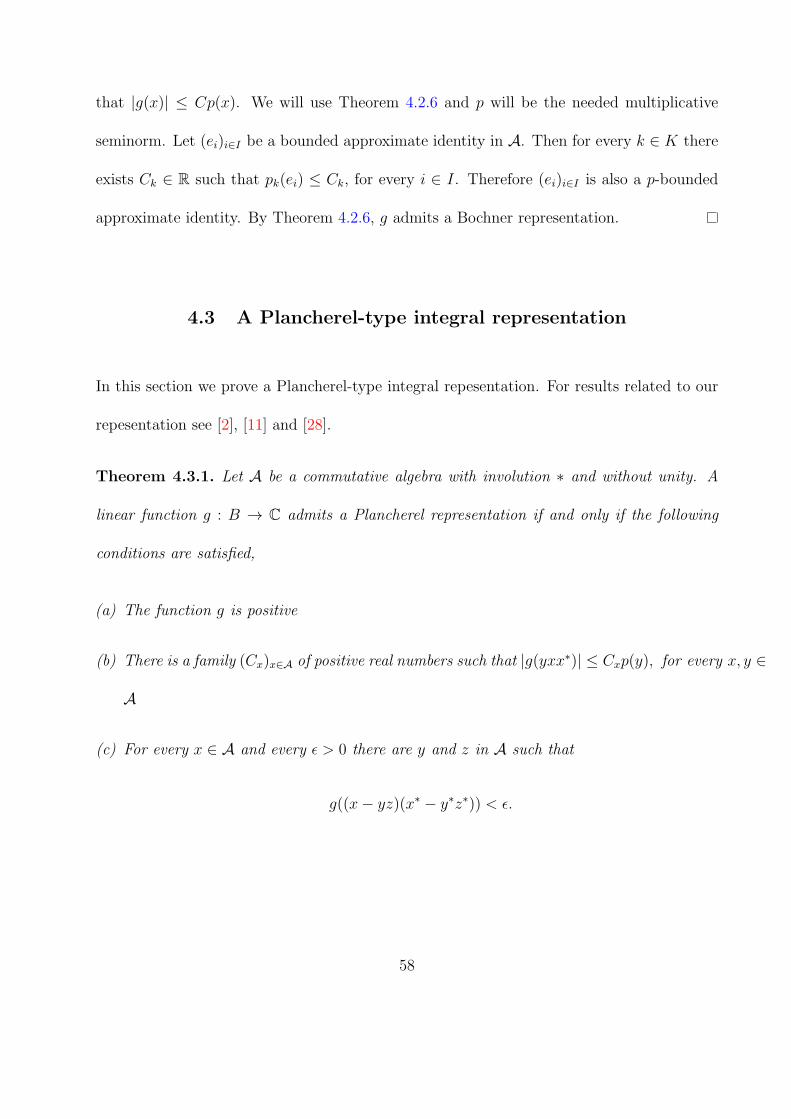
4.3 A Plancherel-type integral representation
In this section we prove a Plancherel-type integral repesentation. For results related to our
repesentation see [2], [11] and [28].
Theorem 4.3.1. Let A be a commutative algebra with involution ∗ and without unity. A
linear function g : B → C admits a Plancherel representation if and only if the following
conditions are satisfied,
(a) The function g is positive
(b) There is a family (Cx)x∈A of positive real numbers such that |g(yxx∗)| ≤ Cxp(y), for every x, y ∈
A
(c) For every x ∈ A and every ϵ > 0 there are y and z in A such that
g((x− yz)(x∗ − y∗z∗)) < ϵ.
58

Proof. For x ∈ A we consider function gx : y 7→ g(yxx∗). Then gx is positive for all x ∈ A.
By Lemma 4.2.5,
|gx(y)|2 = |g(yxx∗)|2 = |g((yx)x∗)|2 ≤ g(xx∗)g(yy∗xx∗) = g(xx∗)gx(yy∗).
Therefore by Lemma 4.2.2, the function gx can be extended to linear positive functional on
Ae by
(gx)e : y + λe 7→ g(yxx∗) + λg(xx∗).
Consequently, we have
|(gx)e(y)| = |g(yxx∗)| ≤ Cxp(y).
The seminorm p can be extended to a seminorm on Ae by pe(x+ λe) = p(x) + |λ|. We will
show that (gx)e satisfies the conditions for Theorem 4.2.1. Note that
|(gx)e(y + λe)| ≤ |g(yxx∗)|+ |λg(xx∗)|
≤ Cxp(y) + |λg(xx∗)|
≤ max{Cx, g(xx∗)}(p(y) + |λ|)
≤ max{Cx, g(xx∗)}p(y + λe).
Hence, (gx)e satisfies the conditions from Theorem 4.2.1. Thus for every x ∈ A there exists
a positive radon measure νx on Ke such that
(gx)e(y + λe) =
∫Ke
ρ(y + λe)dνx(ρ).
59
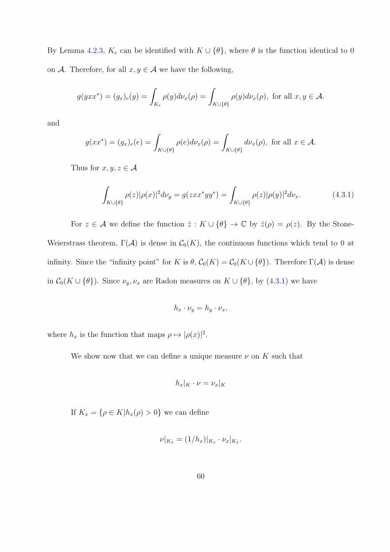
By Lemma 4.2.3, Ke can be identified with K ∪ {θ}, where θ is the function identical to 0
on A. Therefore, for all x, y ∈ A we have the following,
g(yxx∗) = (gx)e(y) =
∫Ke
ρ(y)dνx(ρ) =
∫K∪{θ}
ρ(y)dνx(ρ), for all x, y ∈ A.
and
g(xx∗) = (gx)e(e) =
∫K∪{θ}
ρ(e)dνx(ρ) =
∫K∪{θ}
dνx(ρ), for all x ∈ A.
Thus for x, y, z ∈ A
∫K∪{θ}
ρ(z)|ρ(x)|2dνy = g(zxx∗yy∗) =
∫K∪{θ}
ρ(z)|ρ(y)|2dνx. (4.3.1)
For z ∈ A we define the function z : K ∪ {θ} → C by z(ρ) = ρ(z). By the Stone-
Weierstrass theorem, Γ(A) is dense in C0(K), the continuous functions which tend to 0 at
infinity. Since the “infinity point” for K is θ, C0(K) = C0(K ∪{θ}). Therefore Γ(A) is dense
in C0(K ∪ {θ}). Since νy, νx are Radon measures on K ∪ {θ}, by (4.3.1) we have
hx · νy = hy · νx,
where hx is the function that maps ρ 7→ |ρ(x)|2.
We show now that we can define a unique measure ν on K such that
hx|K · ν = νx|K
If Kx = {ρ ∈ K|hx(ρ) > 0} we can define
ν|Kx = (1/hx)|Kx · νx|Kx .
60

Note that ν is well defined since hx · νy = hy · νx.
Since ρ ≡ 0, we have ∪x∈A
Kx = K
and consequently ν is defined on K.
Note that for all x, y ∈ A,
4xy =∑
τ∈{±1,±i}
τ(x+ τy∗)(x+ τy∗)∗. (4.3.2)
Since g is linear we will find the integral representation for g(xx∗) and use (4.3.2) to show
the integral representation for g(xy).
For every t ∈ A, θ(t) = 0, thus we have
g(txx∗) =
∫K∪{θ}
ρ(t)dνx(ρ)
=
∫K
ρ(t)dνx(ρ)
=
∫K
ρ(t)gx(ρ)dν(ρ)
=
∫K
ρ(t)|ρ(x)|2dν(ρ)
=
∫K
ρ(txx∗)dν(ρ).
Thus for every t, x, y ∈ A and every τ ∈ {±1,±i} we have
g(t(x+ τy∗)(x+ τy∗)∗) =
∫K
ρ(t(x+ τy∗)(x+ τy∗)∗)dν(ρ).
Thus from equation (4.3.2),
g(txy) =∑
τ∈{±1,±i}
τ
4g(t(x+ τy∗)(x∗ + τ y)) (4.3.3)
61

we get
g(txy) = g
t ∑τ∈{±1,±i}
τ
4(x+ τy∗)(x∗ + τ y)
=
∑τ∈{±1,±i}
τ
4g(t(x+ τy∗)(x+ τy∗)∗)
=∑
τ∈{±1,±i}
τ
4
∫K
ρ(t(x+ τy∗)(x+ τy∗)∗)dν(ρ)
=
∫K
ρ
t ∑τ∈{±1,±i}
τ
4(x+ τy∗)(x+ τy∗)∗
dν(ρ)
=
∫K
ρ(txy)dν(ρ).
That is for every x, y, t ∈ A
g(txy) =
∫K
ρ(txy)dν(ρ). (4.3.4)
Now we want to show that, for all x ∈ A, νx({θ}) = 0. Let x ∈ A and ϵ > 0, then there exist
y, z ∈ A such that g((x− yz)(x∗ − y∗z∗)) < ϵ. By (4.3.4) and the integral representation for
gz the following holds,
g(xx∗)−g((x− yz)(x∗ − y∗z∗))
= g(xx∗ − xx∗ + xy∗z∗ + yzx∗ − yzy∗z∗)
= g(xy∗z∗) + g(yzx∗)− g(yy∗zz∗)
=
∫K
ρ(xy∗z∗)dµ(ρ) +
∫K
ρ(yzx∗)dµ(ρ)−∫K∪{θ}
ρ(yy∗)dµz(ρ)
=
∫K
ρ(xy∗z∗)dµ(ρ) +
∫K
ρ(yzx∗)dµ(ρ)−∫K
ρ(yy∗)dµz(ρ)
=
∫K
ρ(xy∗z∗)dµ(ρ) +
∫K
ρ(yzx∗)dµ(ρ)−∫K
ρ(yy∗)|ρ(z)|2dµ(ρ)
62

=
∫K
ρ(xy∗z∗)dµ(ρ) +
∫K
ρ(yzx∗)dµ(ρ)−∫K
ρ(yy∗zz∗)dµ(ρ)
=
∫K
ρ(xy∗z∗ + yzx∗ − yy∗zz∗)dµ(ρ)
=
∫K
ρ(xx∗ − xx∗ + xy∗z∗ + yzx∗ − yy∗zz∗)dµ(ρ)
=
∫K
ρ(xx∗)dµ(ρ)−∫K
ρ(xx∗ + xy∗z∗ + yzx∗ − yy∗zz∗)dµ(ρ)
=
∫K
ρ(xx∗)dµ(ρ)−∫K
ρ((x− yz)(x∗ − y∗z∗))dµ(ρ).
Therefore,
g(xx∗)−∫K
ρ(xx∗)dµ(ρ) = g((x− yz)(x∗ − y∗z∗))−∫K
ρ((x− yz)(x∗ − y∗z∗))dµ(ρ).
Now we return to νx({θ}),
νx({θ}) =∫K∪{θ}
dνx −∫K
dνx
= g(xx∗)−∫K
|ρ(x)|2dν
= g((x− yz)(x∗ − y∗z∗))−∫K
|ρ(x− yz)|2dν(ρ)
≤ g((x− yz)(x∗ − y∗z∗))
< ϵ.
Thus we take ϵ→ 0 and it results that
νx({θ}) = 0.
This means that for every x ∈ A,
63
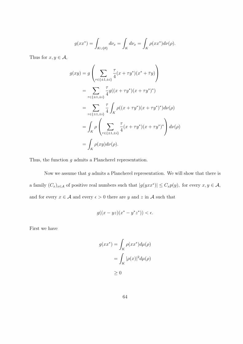
g(xx∗) =
∫K∪{θ}
dνx =
∫K
dνx =
∫K
ρ(xx∗)dν(ρ).
Thus for x, y ∈ A,
g(xy) = g
∑τ∈{±1,±i}
τ
4(x+ τy∗)(x∗ + τ y)
=
∑τ∈{±1,±i}
τ
4g((x+ τy∗)(x+ τy∗)∗)
=∑
τ∈{±1,±i}
τ
4
∫K
ρ((x+ τy∗)(x+ τy∗)∗)dν(ρ)
=
∫K
ρ
∑τ∈{±1,±i}
τ
4(x+ τy∗)(x+ τy∗)∗
dν(ρ)
=
∫K
ρ(xy)dν(ρ).
Thus, the function g admits a Plancherel representation.
Now we assume that g admits a Plancherel representation. We will show that there is
a family (Cx)x∈A of positive real numbers such that |g(yxx∗)| ≤ Cxp(y), for every x, y ∈ A,
and for every x ∈ A and every ϵ > 0 there are y and z in A such that
g((x− yz)(x∗ − y∗z∗)) < ϵ.
First we have
g(xx∗) =
∫K
ρ(xx∗)dµ(ρ)
=
∫K
|ρ(x)|2dµ(ρ)
≥ 0
64

and
|g(yxx∗)| =∣∣∣∣∫K
ρ(y)|ρ(x)|2dµ(ρ)∣∣∣∣
≤(∫
K
|ρ(x)|2dµ(ρ))p(y)
= Cxp(y).
Next we have to show that for every x ∈ A and every ϵ > 0 there are y and z in A
such that
g((x− yz)(x∗ − y∗z∗)) =
∫K
|ρ(x)− ρ(y)ρ(z)|2dµ(ρ) ≤ ϵ.
Fix x ∈ A and ϵ > 0. Since continuous functions with compact support are dense in
L2(K), there exists a continuous function with compact support φ such that∫K
|ρ(x)− φ(ρ)|2dµ(ρ) ≤ ϵ
8.
Let r ∈ supp φ, then there exist s ∈ A such that r(s) = 0. Thus, r(ss∗) = |r(s)|2 > 0. There
exists a neighborhood, Ur, of r such that |t(s)|2 > 0 for every t in Ur. The set {Ur}r∈supp φ
form a cover of supp φ, thus there exists a finite set of rk, 1 ≤ k ≤ n, whose neigborhoods
cover supp φ. Let s1, s2, . . . sn be the corresponding sk’s. Then r(s1s∗1 + . . . + sns
∗n) > 0 for
every r ∈ supp φ.
By the Stone-Weierstrass theorem, Γ(A) is dense in C0(A). Let y = s1s∗1+ . . .+ sns
∗n.
Since the function φyis continuous on K and has compact support, there exists z ∈ A such
that
supρ∈K
∣∣∣∣φ(ρ)ρ(y)− z(ρ)
∣∣∣∣ <√ ϵ
8∫K|ρ(y)|2dµ(ρ)
.
65

Hence,
∫K
|φ(ρ)− ρ(y)ρ(z)|2dµ(ρ) =∫K
|ρ(y)|2∣∣∣∣φ(ρ)ρ(y)
− ρ(z)
∣∣∣∣2 dµ(ρ)≤ ϵ
8∫K|ρ(y)|2dµ(ρ)
∫K
|ρ(y)|2dµ(ρ)
≤ ϵ
8
and consequently
∫K
|ρ(x)− ρ(y)ρ(z)|2dµ(ρ) =∫K
|ρ(x)− φ(ρ) + φ(ρ)− ρ(y)ρ(z)|2dµ(ρ)
≤ 4
(∫K
|ρ(x)− φ(ρ)|2dµ(ρ) +∫K
|φ(ρ)− ρ(y)ρ(z)|2dµ(ρ))
≤ 4( ϵ8+ϵ
8
)= ϵ.
4.4 Back to Bochner
We will now discuss some situations where a function that admits a Plancherel representation
also admits a Bochner representation.
Theorem 4.4.1. Let A be a commutative algebra with involution ∗ and without unity. Let
g : A → C be a positive linear function and p a multiplicative seminorm on A. If there is a
positive real number C such that |g(x)| ≤ Cp(x), for every x ∈ A, and for every x ∈ A and
66

every ϵ > 0 there exists elements y and z in A such that
p(x− yz) < ϵ, (4.4.1)
then g has a Plancherel-type integral representation as in Section 4.3.
If the measure µ from Plancherel representation is finite, then g admits a Bochner-
type integral representation.
Proof. We will use Theorem 4.3.1 to show that g has a Plancherel representation. Consider,
for x, y ∈ A,
|g(yxx∗)| ≤ Cp(yxx∗) ≤ C|p(x)|2p(y) = Cxp(y).
Fix x ∈ A and ϵ > 0. There exist y, z ∈ A such that p(x− yz) <√
1Cϵ. Therefore,
g((x− yz)(x∗ − y∗z∗)) ≤ Cp(x− yz)2 < C
(√1
Cϵ
)2
= ϵ.
Thus by Theorem 4.3.1, g has a Plancherel representation.
Next we will show that g admits a Bochner representation if µ is finite. Suppose that
µ is finite. Let x ∈ A and ϵ > 0. We will show that∣∣g(x)− ∫
Kρ(x)dµ(ρ)
∣∣ < ϵ. There exists
y, z ∈ A such that p(x− yz) < ϵ. Consider
g(x)− g(x− yx) = g(x− x+ yz)
= g(yz)
=
∫K
ρ(yz)dµ(ρ)
=
∫K
ρ(x− x+ yz)dµ(ρ)
67

=
∫K
ρ(x)− ρ(x− yz)dµ(ρ)
=
∫K
ρ(x)dµ(ρ)−∫K
ρ(x− yz)dµ(ρ).
Therefore
g(x)−∫K
ρ(x)dµ(ρ) = g(x− yz)−∫K
ρ(x− yz)dµ(ρ).
So we have the following,∣∣∣∣g(x)− ∫K
ρ(x)dµ(ρ)
∣∣∣∣ = ∣∣∣∣g(x− yz)−∫K
ρ(x− yz)dµ(ρ)
∣∣∣∣≤ |g(x− yz)|+
∫K
|ρ(x− yz)| dµ(ρ)
≤ Cp(x− yz) + p(x− yz)
∫K
dµ(ρ)
= Cµ(K)p(x− yz)
< Cµ(K)ϵ.
Thus we take the limit as ϵ→ 0 and we get that g has a Bochner representation.
The next theorem is another theorem in which we get the Bochner representation
from the Plancherel representation. As you will see, in this case there are more assumptions
on A that will lead to the boundedness of the measure µ.
Theorem 4.4.2. Let A be a commutative algebra with involution ∗ and without unity and
p a multiplicative seminorm on A. Let g : A → C be a positive linear function such that the
following hold,
1. There exists C > 0 such that for every x ∈ A, |g(x)| ≤ Cp(x)
68

2. For every ϵ > 0 and x ∈ A there exists y, z ∈ A such that
p(x− yz) < ϵ.
If there is a sequence (en)n∈N in A such that
1. p(en) ≤ 1, n ∈ N
2. limn→∞ ρ(en) = 1, ρ ∈ K,
then g admits a Bochner-type representation and we have g(x) = limn→∞ g(xen) for every
x ∈ A.
Proof. By Theorem 4.4.1 g admits a Plancherel representation. From the Plancherel repre-
sentation, we have
g(ene∗n) =
∫K
ρ(ene∗n)dµ(ρ) =
∫K
|ρ(en)|2dµ(ρ).
Using that g(ene∗n) ≤ Cp(ene
∗n) ≤ C, lim inf
n→∞|ρ(ej)|2 = 1, and Fatou’s Lemma we obtain
C ≥ lim infn→∞
∫K
|ρ(ej)|2dµ(ρ)
≥∫K
lim infn→∞
|ρ(ej)|2dµ(ρ)
= µ(K).
The measure µ is finite and consequently, according to Theorem 4.4.1, the function g admits
a Bochner-type representation. Now the fact that g(x) = limn→∞ g(xen) is a consequence of
dominated convergence theorem because the function x is µ-integrable for every x ∈ A.
69
CHAPTER 5
PSEUDOQUOTIENTS ON COMMUTATIVE BANACH
ALGEBRAS
The following results are taken from the paper [8].
5.1 Introduction
In this section we recall the construction of pseudoquotients and its basic properties. The
construction of pseudoqutients was introduced in [21] under the name of “generalized quo-
tients”. The motivation for the idea, early developments, and later modifications, are dis-
cussed in [22]. The construction of pseudoquotients has desirable properties. For instance, it
preserves the algebraic structure of X and has good topological properties. There is growing
evidence that pseudoquotients can be a useful tool (see, for example, [5], [6], or [7]).
Let X be a nonempty set and let S be a commutative semigroup acting on X injec-
tively. The relation
(x, φ) ∼ (y, ψ) if ψx = φy
70

is an equivalence in X×S. We define B(X,S) = (X×S)/∼. Elements of B(X,S) are called
pseudoquotients. The equivalence class of (x, φ) will be denoted by xφ. Thus
x
φ=y
ψmeans ψx = φy.
Elements of X can be identified with elements of B(X,S) via the embedding ι : X →
B(X,S) defined by
ι(x) =φx
φ,
where φ is an arbitrary element of S. The action of S can be extended to B(X,S) via
φx
ψ=φx
ψ.
If φ xψ= ι(y), for some y ∈ X, we simply write φ x
ψ∈ X and φ x
ψ= y. For instance, we have
φ xφ= x.
In the case X is a topological space or a convergence space and S is a commutative
semigroup of continuous injections acting on X, then we can define a convergence in B(X,S)
as follows: If, for a sequence Fn ∈ B(X,S), there exist φ ∈ S and F ∈ B(X,S) such that
φFn, φF ∈ X, for all n ∈ N, and φFn → φF in X, then we write FnI→ F in B(X,S). In
other words, FnI→ F in B(X,S) if
Fn =xnφ, F =
x
φ, and xn → x in X,
for some xn, x ∈ X and φ ∈ S.
This convergence is sometimes referred to as type I convergence. It is quite natural,
but it need not be topological. For this reason we prefer to use the convergence defined as
71

follows: Fn → F in B(X,S) if every subsequence (Fpn) of (Fn) has a subsequence (Fqn) such
that FqnI→ F .
It is easy to show that the embedding ι : X → B(X,S), as well as the extension of
any φ ∈ S to a map φ : B(X,S) → B(X,S) defined above, are continuous.
The set of all positive linear functionals on an algebra A is denoted by P(A). The
following theorem (attributed to Maltese in [15]) describes P(A) in terms of measures on A.
We say A has a symmetric involution, if
x∗ = x, for all x ∈ A.
Theorem 5.1.1. Let A be a commutative Banach algebra with a bounded approximate iden-
tity and an isometric and symmetric involution. Let f be a linear functional on A. Then
f ∈ P(A) if and only if
f(x) =
∫Ax(ξ)dµf (ξ),
for all x ∈ A, with respect to a unique positive Radon measure on A of total variation ∥f∥.
Let F : P(A) → Mb+(A) be the map defined by Maltese’s theorem, that is, F(f) =
µf . In terms of the introduced notation, Theorem 5.1.1 states that F is an isometry between
P(A) and Mb+(A). In this chapter we give conditions under which P(A) can be extended to
a space of pseudoquotients B(P(A),S) such that F can be extended to a bijection between
B(P(A),S) and M+(A).
72

In Section 5.2 we formulate and prove the main result of this chapter. In Section
5.3 we discuss some examples. We also show that the result in [6] is a special case of the
construction presented here.
5.2 An extension of Maltese’s theorem
In this section we will assumeA to be a nonunital commutative Banach algebra with bounded
approximate identities and an isometric and symmetric involution. In addition, we assume
that A satisfies the following condition:
Σ There exists a sequence a1, a2, . . . ∈ A such that a1, a2, . . . ∈ K(A) and for every ξ ∈ A
there is an n such that an(ξ) = 0.
The following are some examples of spaces where Σ is satisfied.
Example 5.2.1 (Normal algebras). Let A be a commutative Banach algebra. We say that
A is normal [17], if for every compact K ⊂ A and closed E ⊂ A such that K ∩E = ∅, there
exists x ∈ A such that
x(ξ) = 1 for ξ ∈ K and x(ξ) = 0 for ξ ∈ E.
If A is a normal commutative Banach algebra and A is σ-compact, then A satisfies
condition Σ. Indeed, if A is σ-compact, there are compact sets Kn ⊂ A such that A =
73
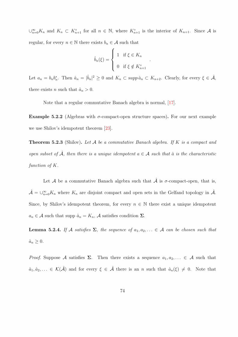
∪∞n=0Kn and Kn ⊂ K◦
n+1 for all n ∈ N, where K◦n+1 is the interior of Kn+1. Since A is
regular, for every n ∈ N there exists bn ∈ A such that
bn(ξ) =
1 if ξ ∈ Kn
0 if ξ /∈ K◦n+1
.
Let an = bnb∗n. Then an = |bn|2 ≥ 0 and Kn ⊂ supp an ⊂ Kn+2. Clearly, for every ξ ∈ A,
there exists n such that an > 0.
Note that a regular commutative Banach algebra is normal, [17].
Example 5.2.2 (Algebras with σ-compact-open structure spaces). For our next example
we use Shilov’s idempotent theorem [23].
Theorem 5.2.3 (Shilov). Let A be a commutative Banach algebra. If K is a compact and
open subset of A, then there is a unique idempotent a ∈ A such that a is the characteristic
function of K.
Let A be a commutative Banach algebra such that A is σ-compact-open, that is,
A = ∪∞n=0Kn where Kn are disjoint compact and open sets in the Gelfand topology in A.
Since, by Shilov’s idempotent theorem, for every n ∈ N there exist a unique idempotent
an ∈ A such that supp an = Kn, A satisfies condition Σ.
Lemma 5.2.4. If A satisfies Σ, the sequence of a1, a2, . . . ∈ A can be chosen such that
an ≥ 0.
Proof. Suppose A satisfies Σ. Then there exists a sequence a1, a2, . . . ∈ A such that
a1, a2, . . . ∈ K(A) and for every ξ ∈ A there is an n such that an(ξ) = 0. Note that
74
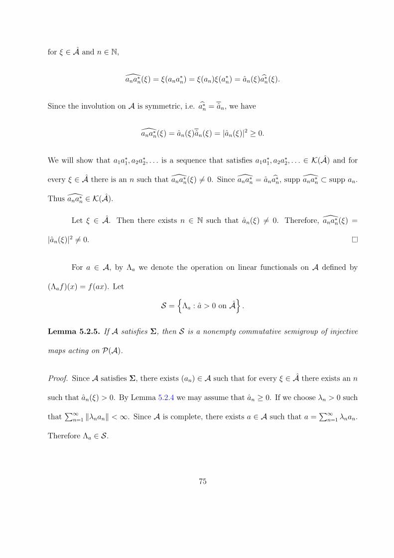
for ξ ∈ A and n ∈ N,
ana∗n(ξ) = ξ(ana∗n) = ξ(an)ξ(a
∗n) = an(ξ)a∗n(ξ).
Since the involution on A is symmetric, i.e. a∗n = an, we have
ana∗n(ξ) = an(ξ)an(ξ) = |an(ξ)|2 ≥ 0.
We will show that a1a∗1, a2a
∗2, . . . is a sequence that satisfies a1a
∗1, a2a
∗2, . . . ∈ K(A) and for
every ξ ∈ A there is an n such that ana∗n(ξ) = 0. Since ana∗n = ana∗n, supp ana∗n ⊂ supp an.
Thus ana∗n ∈ K(A).
Let ξ ∈ A. Then there exists n ∈ N such that an(ξ) = 0. Therefore, ana∗n(ξ) =
|an(ξ)|2 = 0.
For a ∈ A, by Λa we denote the operation on linear functionals on A defined by
(Λaf)(x) = f(ax). Let
S ={Λa : a > 0 on A
}.
Lemma 5.2.5. If A satisfies Σ, then S is a nonempty commutative semigroup of injective
maps acting on P(A).
Proof. Since A satisfies Σ, there exists (an) ∈ A such that for every ξ ∈ A there exists an n
such that an(ξ) > 0. By Lemma 5.2.4 we may assume that an ≥ 0. If we choose λn > 0 such
that∑∞
n=1 ∥λnan∥ < ∞. Since A is complete, there exists a ∈ A such that a =∑∞
n=1 λnan.
Therefore Λa ∈ S.
75

Clearly, S is a commutative semigroup because A is commutative. Let f ∈ P(A) and
Λa ∈ S. By Maltese’s theorem [15], f(x) =
∫Ax(ξ)dµ(ξ) for some µ ∈ Mb
+(A). Thus
(Λaf)(x) = f(ax) =
∫Aax(ξ)dµ(ξ) =
∫Ax(ξ)a(ξ)dµ(ξ).
Note that a is a positive bounded function on A. Since a(ξ) > 0 for all ξ ∈ A, µ = aµ ∈
Mb+(A) and Λaf(x) =
∫A x(ξ)dµ(ξ). By Maltese’s theorem [15], Λaf ∈ P(A).
If Λaf = 0, then
0 = f(ax) =
∫Aax(ξ)dµ(ξ) =
∫Ax(ξ)a(ξ)dµ(ξ),
for all x in A. By the Stone-Weierstrass theorem, Γ(A) is dense in C0(A). Therefore aµ = 0
which implies µ = 0, because a > 0. Thus
f(x) =
∫Ax(ξ)dµ(ξ) = 0.
Hence Λa is injective.
The map F : P(A) → Mb+(A) defined by Maltese’s theorem, can be extended to a
map F : B(P(A),S) → M+(A) in the natural way:
F(f
Λa
)=
F(f)
a=
1
aµf . (5.2.1)
It is clear that F is well-defined.
Theorem 5.2.6. Let A be a nonunital commutative Banach algebra with a bounded approxi-
mate identity and an isometric and symmetric involution. If A satisfies Σ, then the extended
F defined by (5.2.1) is an bijection from B(P(A),S) to M+(A).
76

Proof. First we will show that F is injective. Suppose that F(f
Λa
)= 0, that is
1
aµf = 0,
which implies µf = 0. Therefore f(x) = 0 because f(x) =
∫Ax(ξ)dµf (ξ). So,
f
Λa= 0 and
F is injective.
Next we will show that F is surjective. Let µ ∈ M+(A). There are an ∈ A such
that an ≥ 0, supp an is compact, and such that for every ξ ∈ A there exists an n such that
an(ξ) > 0. Then anµ is a finite positive Radon measure on A for every n ∈ N. There exist
positive numbers λ1, λ2, . . . such that∑∞
n=1 λnanµ defines a finite positive Radon measure
on A and∑∞
n=1 ∥λnan∥ <∞. By Maltese’s theorem there exists f ∈ P(A) such that
µf =∞∑n=1
λnanµ.
Since A is complete there exists a ∈ A such that a =∑∞
n=1 λnan. Then Λa ∈ S and∑∞n=1 λnanµ = aµ. Thus
F(f
Λa
)=µfa
=aµ
a= µ.
Theorem 5.2.7. The map F : B(P(A),S) → M+(A) is a sequential homeomorphism.
Proof. If FnI→ F in B(P(A),S), then Fn =
fnΛa
, F =f
Λa, and fn → f in P(A) for some
fn, f ∈ P(A), where fn → f means fn(x) → f(x) for all x ∈ A. Consequently,∫Ax(ξ)dµfn(ξ) →
∫Ax(ξ)dµf (ξ)
for all x ∈ A. Since the involution in A is symmetric and Γ(A) = {x : x ∈ A} strongly
separates points in A (see, for example, Theorem 2.2.7 in [16]). Thus by the Stone-Weirstrass
77

theorem Γ(A) is dense in C0(A). We obtain
∫Aφ(ξ)dµfn(ξ) →
∫Aφ(ξ)dµf (ξ)
for all φ ∈ K(A). Therefore,
∫Aφ(ξ)
dµfn(ξ)
a(ξ)→∫Aφ(ξ)
dµf (ξ)
a(ξ)
for all φ ∈ K(A), which means that F(Fn) → F(F ) in M+(A).
Now assume µn, µ ∈ M+(A) and
∫Aφ(ξ)dµn(ξ) →
∫Aφ(ξ)dµ(ξ)
for all φ ∈ K(A). There exist λk > 0, k ∈ N, such that∑∞
k=1 λkakµn is a finite measure for
all n ∈ N and Λa ∈ S, where a =∑∞
k=1 λkak. Let
fn = F−1
(∞∑k=1
λkakµn
)= F−1(aµn)
and
f = F−1
(∞∑k=1
λkakµ
)= F−1(aµ).
Then F−1(µn) = F−1
(aµna
)=fnΛa
and F−1(µ) = F−1
(aµ
a
)=
f
Λa. Moreover,
fn(x) =
∫Ax(ξ)a(ξ)dµn(ξ) →
∫Ax(ξ)a(ξ)dµ(ξ) = f(x)
for every x ∈ A. ThereforefkΛa
I→ f
Λain B(P(A),S).
78

5.3 Examples
In this section we give some examples of spaces where the assumptions of Theorem 5.2.6 are
satisfied.
Example 5.3.1. Locally compact groups
Let G be a locally compact abelian group. A continuous function f : G→ C is called
positive definite ifn∑
k,l=1
ckclf(x−1l xk) ≥ 0
for all c1, . . . , cn ∈ C and x1, . . . , xn ∈ G for any n ∈ N. We denote the cone of positive
definite functions on G by P+(G). A character α on G is a continuous homomorphism
from G into the unit circle group T. Let G denote the group of characters. By Bochner’s
theorem [13], f ∈ P+(G) if and only if there exists a unique bounded positive Radon measure
µf on G such that
f(x) =
∫G
xdµf .
In [6] it was shown that, if G is σ-compact, then the map f 7→ µf defined by Bochner’s
theorem can be extended to a map from a space of pseudoquotients to all positive measures
on G. That space of pseudoquotients was B(P+(G),S) where
S ={φ ∈ L1(G) : φ(ξ) > 0 for all ξ ∈ G
}.
We will show that this extension is a special case of the extension presented in this note.
79

Since the convolution algebra L1(G) is regular, it satisfies Σ, as indicated in 5.2.1.
For α ∈ G we define φα : L1(G) → C by
φα(f) =
∫G
f(x)α(x)dx,
where dx indicates the integral with respect to the Haar measure on G. The map α 7→ φα
is a bijection from G onto L1(G) (see, for example, [16]). This allows us to identify M+(G)
and M+(L1(G)). If f is a positive definite function on G, we define a positive functional on
L1(G) by
F (ψ) =
∫G
f(x)ψ(x)dx
and a map from B(P+(G),S) to B(L1(G),S) by f
ψ7→ F
Λψ, where ψ(x) = ψ(x−1). We will
show that F is positive.
F (ψ ∗ ψ∗) =
∫G
ψ ∗ ψ∗(x)f(x)dx
=
∫G
∫G
ψ(xy−1)ψ∗(y)f(x)dydx
=
∫G
∫G
ψ(xy−1)ψ(y−1)f(x)dydx
=
∫G
∫G
ψ(x)ψ(y−1)f(xy)dydx
=
∫G
∫G
ψ(x)ψ(y)f(xy−1)dydx.
Riemann sums for this integral are of the formn∑
k,l=1
ckclf(x−1l xk) which are nonnegative since
f is positive definite. Therefore F (ψ ∗ ψ∗) ≥ 0. Thus for all ψ in L1(G),
F (ψ) =
∫L1(G)
φα(ψ)dµF (α)
80
=
∫L1(G)
∫G
ψ(x)α(x)dxdµF (α)
=
∫G
∫G
ψ(x)α(x)dµf (α)dx.
Therefore for all ψ in L1(G),
∫G
ψ(x)f(x)dx =
∫G
∫G
ψ(x)α(x)dµf (α)dx
which implies,
f(x) =
∫G
α(x)dµf (α).
81

LIST OF REFERENCES
[1] D. Atanasiu, Un theoreme du type Bochner-Godement et le probleme des moments, J.Func. Anal. 92, (1990), 92–102.
[2] D. Atanasiu, Bi-fonctions moment, Math.Scand. 69, (1991), 152–160.
[3] D. Atanasiu, A Levy−Khinchine Formula for Semigroups and Related Problems: AnAdapted Spaces Approach J. Math. Anal. Appl., Vol. 198, Issue 1, (1996), 237-247
[4] D. Atanasiu, Spectral Measures on Compacts of Characters of a Semigroup in VectorMeasures, Integration and Related Topics, Operator Theory: Advances and Applica-tions 201, Birkhauser, Basel, (2010), 41–49.
[5] D. Atanasiu and P. Mikusinski, The Fourier transform of Levy measures on a semigroup,Integral Transform. Spec. Funct. 19, (2008), 537–543.
[6] D. Atanasiu and P. Mikusinski, Fourier transform of Radon measures on locally compactgroups, Integral Transform. Spec. Funct. 21, (2010), 815–821.
[7] D. Atanasiu, P. Mikusinski, and D. Nemzer, An algebraic approach to tempered distri-butions, J. Math. Anal. Appl. 384, (2011), 307–319.
[8] D. Atanasiu, P. Mikusinski, A. Siple, Pseudoquotients on commutative Banach algebras,Banach J. Math. Anal. 8, (2014), 60-66.
[9] C. Berg, J. P. R. Christensen, P. Ressel, Harmonic analysis on semigroups: Theory ofpositive definite and related functions, Springer-Verlag, New York, (1984).
[10] C. Berg and P. H. Maserick, Exponentially bounded positive definite functions, IllinoisJ. Math., Vol. 28, Issue 1, (1984), 162–179.
[11] J. Dieudonne, Treatise on Analysis, Volume II, Academic Press, (1970).
[12] R. Doran and V. Belfi, Characterizations of C∗ Algebras: the Gelfand Naimark Theo-rems, M. Dekker, New York, (1986).
[13] G.B. Folland, A Course in Abstract Harmonic Analysis, CRC Press, Boca Raton, (1995).
[14] M. Fragoulopoulou, Abstract Bochner-Weil-Raikov theorem in topological algebras, Bull.Austral. Math. Soc. 26, (1982), 39–44.
82

[15] M. Fragoulopoulou, Topological Algebras with Involution, North-Holland MathematicsStudies 200, Elsevier Science B.V., Amsterdam, (2005).
[16] E. Kaniuth, A Course in Commutative Banach Algebras, Springer, New York, (2008).
[17] R. Larsen, Banach Algebras an Introduction, Marcel Dekker Inc., New York, (1973).
[18] G. Lumer, Bochner’s theorem, states, and the Fourier transforms of measures, StudiaMath. 46, (1973), 135–140.
[19] G. Maltese, A representation theorem for positive functionals on Involution Alge-bras(Revisited), Bollettino U.M.I. 7, (1994), 431–438.
[20] P. H. Maserick and F. H. Szafraniec Equivalent definitions of positive definiteness.,Pacific J. Math. Vol. 110, Num. 2, (1984), 315–324.
[21] P. Mikusinski, Generalized quotients with applications in analysis, Methods Appl. Anal.10, (2003), 377–386.
[22] P. Mikusinski, Boehmians and pseudoquotients, Appl. Math. Inf. Sci. 5, (2011), 1–13.
[23] T. W. Palmer, Banach algebras and the general theory of *-algebras, Vol. I, Cambridge,New York (1994)
[24] P. Ressel, Integral representations on convex semigroups, Math. Scand. 61, (1987), 93–111.
[25] P. Ressel, De Finetti-type theorems: An analytical appoach, The Annals of Probability12, (1985), 898–922.
[26] P. Ressel, Exchangeability and semigroups, Rendiconti di matematica, Serie VII, 28(2008), 63-81.
[27] P. Ressel and W. J. Ricker, Semigroup representations, positive definite functions andabelian C∗-algebras, Proc. Amer. Math. Soc. 126, (1998), 2949–2955.
[28] J. Stochel, The Bochner type theorem for *-definite kernels on abelian *-semigroupswithout neutral element in Dilatation Theory, Toeplitz Operators and other Topics,(Timioara/Herculane, 1982), 345362, Oper. Theory Adv. Appl., 11, Birkhuser, Basel,(1983).
83