REMOTE SENSING OF ENVIRONMENT 8:127-150 (1979) 127

Red and Photographic Infrared Linear Combinations for Monitoring Vegetation

COMPTON J. TUCKER

Earth Resources Branch, NASA/Goddard Space Fligftt Center, Greenbelt, Maryland 20771

In situ collected spectrometer data were used to evaluate and quantify the relationships between various linear combinations of red and photographic infrared radiances and experimental plot biomass, leaf water content, and chlorophyll content. The radiance variables evaluated included the red and photographic infrared (IR) radiance and the linear combinations of the IR/red ratio, the square root of the IR/red ratio, the IR-red difference, the vegetation index, and the transfonned vegetation index. In addition, the corresponding green and red linear combinations were evaluated for comparative purposes. Three data sets were used from June, September, and October sampling periods.

Regression analysis showed the increased utility of the IR and red linear combinations vis-a-vis the same green and red linear combinations. The red and IR linear combinations had 7% and 14% greater regression significance than the green and red linear combinations for the June and September sampling periods, respectively.

The vegetation index, transfonned vegetation index, and square root of the IR/ red ratio were the most significant, followed closely by the IR/red ratio. Less than a 6% difference separated the highest and lowest of these four IR and red linear combinations. The use of these linear combinations was shown to be sensitive primarily to the green leaf area or green leaf biomass. As such, these linear combinations of the red and photographic IR radiances can be employed to monitor the photosynthetically active biomass of plant canopies.

Introduction

The use of photographic infrared (IR) and red linear combinations for monitor­ing vegetation biomass and physiological status have recently become common in the remote sensing community. Accom­panying this increased usage, however, has been a lack of detailed analyses con­cerning limitations of these data and their application(s) to vegetation monitor­ing. Quantitative information regarding the various IR and red linear combina­tions and the constraints involved in the use of these methods will enable more advantageous application of these tech­niques. It will also prevent overambitious use of these techniques when other methods would be more applicable. This article examines ground-collected grass

CElsevier North Holland Inc., 1979

canopy spectra in an attempt to quantify the relationship between the IR and red linear combinations and properties of plant canopies.

Previous Work

The use of a near-infrared/red ratio method for estimating biomass or leaf area index was first reported by Jordan (1969) who used a radiance ratio of 0.800/0.675 JLm to derive the leaf area index for forest canopies in a tropical rain forest. This application of the IR/red ratio used the transmitted light at these wavelengths, sensed on the forest floor Gordan, 1969). Subsequent work was reported by Pearson and Miller (1972) who developed a hand-held spectral radiometer for estimating grass

0034-4257/79/C1lJJ127 + 24$01. 75

128

canopy biomass. The instrumentation aspect of the hand-held radiometer is described in Pearson et al. (1976).

Colwell (1973, 1974) presented a de­tailed study of bidirectional spectral re­flectance of grass canopies. He con­cluded that the IR/red ratio was effec­tive in somewhat normalizing the effect of soil background reflectance variation(s) and was useful for estimating biomass. Colwell also cautioned that the IR/red ratios may worsen angular effects rather than alleviate them under certain conditions. Smith and Oliver (1974) have corroborated several of Colwell's (1973, 1974) conclusions using a stochastic canopy model versus Colwell's use of Suits' (1972) deterministic canopy model.

The IR / red ratio method has been applied to LANDSAT image analysis of range biomass by Rouse et al. (1973, 1974), Carneggie et al. (1974), Johnson (1976), and Maxwell (1976), among others.

Carneggie et al. (1974) used a ratio of LANDSAT MSS7/MSSS and found that the ratio curves, plotted as a function of time, peaked during the period of great­est forage production. Thereafter, the curves fell off Signalling the period of drying follOwing the maximum green period for their California study site. Once the curves leveled off, Carneggie et al. (1974) concluded that all annual vegetation had dried.

Rouse et al. (1973, 1974) analyzed LANDSAT MSS data and developed what they referred to as the vegetation index (VI) and transformed vegetation in­dex (TVI). They found that although a simple ratio of MSS7/MSSS could be used as a measurement of relative green­ness, location and cycle deviations would introduce a large error component. The

C. J. TUCKER

difference of the MSS7 - MSSS radiance values, normalized over the sum of MSS7 + MSSS, was used as an index value and was christened the VI.

VI = MSS7 - MSSS (1) MSS7+MSSS .

To avoid working with negative ratio values and the possibility that the vari­ances of the ratio would be proportional to the mean values (Le., a Poisson distrib­ution) the constant of O.S was added and a square-root transformation was applied to the VI.

TVI = YVI +O.S (2)

The VI and TVI were then applied to LANDSAT data. MSS bands 6 and 7 were both evaluated as the near-infrared band. Rouse et al. (1974) reached several conclusions: (1) LANDSAT VI and TVI methods could be used to monitor range­lands and wheat crops; (2) the close rela­tionship between green biomass and TVI should allow researchers to follow crop development as ground cover, biomass, and leaf area indices increase; (3) pheno­logical inferences could poSSibly be gleaned for certain crops or range types and used to monitor these types of vege­tation (Rouse et al., 1974).

Johnston (1976) and Maxwell (1976) also analyzed LANDSAT imagery using ratio methods. They concluded that the ratio of MSS6/MSSS was slightly more statistically Significant than MSS7/MSSS and that both ratios were useful in moni­toring green biomass. An explanation of the apparent greater utility of MSS6 versus MSS7 for rangeland biomass estimation in low biomass situations based upon soil-green-vegetation

PHOTOCOMBINATIONS FOR MONITORING VEGETATION 129

spectral contrasts has been proposed by Tucker and Miller (1977).

Other researchers have also used the VI for LANDSAT analyses. Blair and Baumgardner (1977) monitored several hardwood forest sites using LANDSAT imagery. They used the VI, which they refer to as the "band ratio parameter," and found that the greenwave effect could be monitored for these vegetation types using LANDSAT imagery.

Ashley and Rea (1975) reported how LANDSAT MSS5 and MSS7 data were used to depict phenological change. They also used the VI and found that it in­creased with foliage development and decreased with senescence. The VI was found to reduce influencing multiplica­tive effects such as solar elevation dif­ferences between overpasses (Ashley and Rea, 1975).

In addition to the above reviewed LANDSAT analyses, Kauth and Thomas (1976) and Richardson and Wiegand (1977) have proposed LANDSAT vegeta­tional analytical methods using, at least in part, IR and red linear combinations.

Richardson and Wiegand (1977) have proposed a departure from the soil back­round line with the perpendicular vege­tation index (PVI):

PVI=

X V(Re~il - Re<iveg)2 + (I1\oil - Il\.eg)2 ,

(3)

where Re~il is the soil background red reflectance or radiance, Re<iveg is the vegetation background red reflectance or radiance, I1\oil is the soil background IR reflectance or radiance, Il\.eg is the vegetation background IR reflectance or radiance.

Kauth and Thomas (1976) have devel-

oped a technique for transforming LANDSAT MSS information in four-di­mension data space using the four MSS bands. From this, a soil brightness index (SBI) and green vegetation index (GVI) were calculated as follows:

SBI = 0.43 *MSS4 + O.63*MSS5

+ 0.59*MSS6 + 0.26*MSS7 (4)

and

GVI = - 0.29 MSS4 - 0.56 MSS5

+0.60 MSS6 + 0.49 MSS7. (5)

Note that all the SBI-independent vari­able coefficients are poSitive, while the GVI-independent variables MSS4 and MSS5 are negative. The SBI establishes the data space of soils and the GVI de­parts from it, in a negative or absorptive fashion with MSS4 and MSS5, approxi­mately the same coefficients for MSS6 for both models, and a positive departure for MSS7. This also follows from Fig. l.

Deering (1978), in a recent and com­prehensive analysis of LANDSAT range­land biomass monitoring, has reported that the VI and TVI approaches he evaluated using MSS6 were slightly more Significant with respect to green biomass than the PVI of Richardson and Wiegand (1977) and the GVI of Kauth and Thomas (1976). In addition, Deering (1978) re­ported that the denominator of the VI and TVI (i.e., MSS5 + MSS6 or MSS5 + MSS7) were highly correlated (r > 0.95) to Kauth and Thomas' (1976) soil bright­ness index (SBI).

The majority of IR and red linear com­bination work has used LANDSAT data. Kanemasu (1974), however, reports on a ground-based reflectance study of crop types where various ratios were investi­gated. Wheat, sorghum, and soybean plots were monitored periodically during

130 C. J. TUCKER

~r-------------------------------------~

45.

40

#- 35

GREEN VEGETATION PLOT 20074 (TOTAL DRY BIOMASS = 530 g:m 2)

\ lj 30. Z

DRY SOIL PLOT _

;:: 25.

U ~ 20. u.. ~ 15

SAME SOIL, \ _---------

ONLY WET_\------- _------ _-------

---~--~--. ---- .--. --5. -:~.:::::

10

WAVELENGTH (/1m)

FIGURE 1. Spectral reflectances for dry soil, wet soil, and asymptotic green reflectance. The dry soil and wet soil curves are the average of five bare soil plots measured when dry and wet, respectively. The asymptotic green reflectance curve is from a plot of blue grarna grass having a total dry biomass of 530 g/m2 (from Tucker and Miller, 1977).

the growing season using a spectrometer. Kanemasu (1974) concluded the 0.545/0.655-fJom wavebands provided useful information regardless of crop type. For all crops studied, the green/red ratio closely followed crop growth and development and appeared to be more desirable than the near-in­frared reflectance as an index of growth. The green/red ratio will be evaluated in this paper also.

Recent works by Nalepka et al. (1977) and Tucker et al. (1979) have used IR and red data to forecast winter wheat yields and monitor agricultural crop vigor and condition, respectively. Nalepka et al. (1977) evaluated various green measures using LANDSAT data and con­cluded that most are useful but stress that no new information is created. Tucker et al. (1979) monitored several crop types using a hand-held radiometer.

Basic Properties of the IR and Red Radiances with Respect to Green Vegetation

It is perhaps prudent to briefly review the basic properties of the IR and red radiances with respect to green vegeta­tion before embarking on a detailed anal­ysis of the various linear combinations.

The red radiance exhibits the nonlin­ear inverse relationship between in­tegrated spectral radiance and green bio­mass, while the near-infrared component exhibits a nonlinear direct relationship.

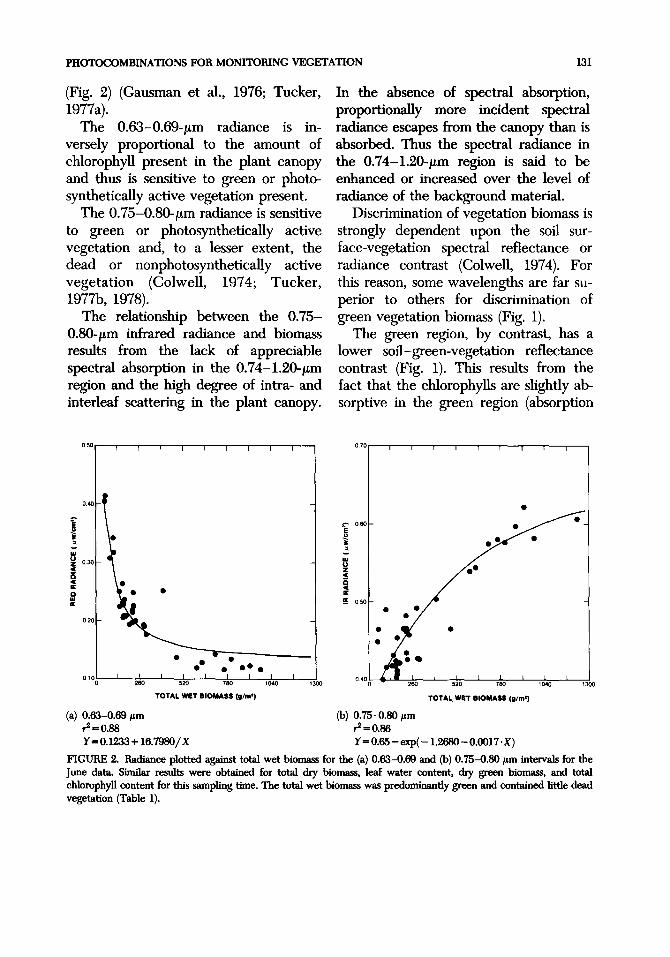
The relationship between the 0.63-0.69-!un radiance and green biomass re­sults from strong spectral absorption of incident radiation by the chlorophylls. It is apparent that a spectral radiance asymptote is more quickly reached for the 0.63-0.69-fJom red radiance than the 0.75-0.80-fJom near-infrared radiance

PHOTOCOMBINATIONS FOR MONITORING VEGETATION 131

(Fig. 2) (Gausman et al., 1976; Tucker, 1977a).

The 0.63-0.69-tJ.m radiance is in­versely proportional to the amount of chlorophyll present in the plant canopy and thus is sensitive to green or photo­synthetically active vegetation present.

The 0.75-0.80-tJ.m radiance is sensitive to green or photosynthetically active vegetation and, to a lesser extent, the dead or nonphotosynthetically active vegetation (Colwell, 1974; Tucker, 1977b, 1978).

The relationship between the 0.75-O.80-tJ.m infrared radiance and biomass results from the lack of appreciable spectral absorption in the 0.74-1.20-tJ.m region and the high degree of intra- and interleaf scattering in the plant canopy.

I ,:; .. U 030 Z :! D c .. D .. ..

020

(a) 0.63-0.69 I'm ,.2-=0.88

•

• • •• • ••• TOTAL WET BIOMASS (g/m')

Y-O.l233+ 16.7980jX

In the absence of spectral absorption, proportionally more incident spectral radiance escapes from the canopy than is absorbed. Thus the spectral radiance in the 0.74-1.20-tJ.m region is said to be enhanced or increased over the level of radiance of the background material.

Discrimination of vegetation biomass is strongly dependent upon the soil sur­face-vegetation spectral reflectance or radiance contrast (Colwell, 1974). For this reason, some wavelengths are far su­perior to others for discrimination of green vegetation biomass (Fig. 1).

The green region, by contrast, has a lower soil-green-vegetation reflectance contrast (Fig. 1). This results from the fact that the chlorophylls are slightly ab­sorptive in the green region (absorption

'f 060

lj ,:; .. u z :! D C .. !!5 oso

• • • • • •

o 40~0 -+J----=-----'----;c52!;;cO----l-..!::760~-'-----:-;'040b::--'-----"d300

TOTAL. WET BIOMASS (g/m')

(b) 0.75-0.80 I'm ,.2=0.86 Y=O.65-exp( -1.2680-0.0017 'X)

F1GURE 2. Radiance plotted against total wet biomass for the (a) 0.63-0.69 and (b) 0.75-0.80 I'm intervals for the June data. Similar results were obtained for total dry biomass, leaf water content, dry green biomass, and total chlorophyll content for this sampling time. The total wet biomass was predominantly green and contained little dead vegetation (Table 1).

132

coefficients--lO), while much more ab­sorptive in the red region (absorption coefficients of --40-90) (Salisbury and Ross, 1969). The relationship between the green radiance and green biomass is similar to the same relationship between the red radiance and green biomass (Figs. 2a and 3).

Description of Research Undertaken

The work reported herein examines ground-collected in situ spectrometer data, evaluates the green/red ratio method of Kanemasu (1974), and con­trasts that with the IR/ red ratio method(s) to determine which are super­ior for the June, September, and October data sets. The utility of the various green vegetation measures using the different

.. o ~ ~ II: Z .. .. II: CI

• •• • •• •••

TOTAL WET alOMASS (g/m')

(a) 0.52-0.60 pm r=0.79 Y=0.237 + 12.129/ X June data

•

c. J. TUCKER

IR and red linear combinations are also evaluated.

Methods and Analysis

The data used in this evaluation have all been previously described and are not redescribed in this report. The June and September data sets are described in Tucker and Maxwell (1976), while the October data is described in Tucker (1978).

The narrow bandwidth radiance curves (0.005-,um bandWidth) were numerically integrated to approximate three bandwidths: 0.52-0.60 ,urn for the green, 0.63-0.69 ,urn for the red, and 0.75-0.80 ,urn in the photographic in­frared. The radiance curves resulted from the product of the spectral reflectance

E • ~ oso • ~ • • - • • w -. • u • - • z .. , • • 0 .. • • a: •• • z • w • , • • w II: 040 •• • CI .,

• • • • • •

030 240 320 400

TOTAL DRY BIOMASS (vim')

(b) 0.52-0.60 pm r=0.14 September data

FIGURE 3. Comparisons between the green radiance (0.52-0.60 pm) and the green/red radiance ratio. Refer to Tables 2 and 3 for the r values associated with this portion of the analysis and Figs. 4c, 5c, and 6c for comparisons to the IR / red ratio for the same data sets.

PHOTOCOMBINATIONS FOR MONITORING VEGETATION 133

0.60 I I I I I I I I I

20

, . ~ • 050 r- • • -i • 0

•• ;: .. - c • ••• • 0: 16 w Q 0 '. • W Z • 0: ~ • Z Q • • W C • • W 0: •• 0: Z • •• • CI 14 W 040 l- • -W • 0: • CI

• , • 1.2 • • • • • •

030 I I I I I I I • I I 10 0 40 80 120 180 200 0 260 520 760 1040 1300

LIAF WATER CONTENT ("m') TOTAL WET BIOMASS (11m')

(C) 0.52-0.60 j.Lm (d) r-=0.82 r=O.33 Y=2.2-exp(0.1OBI-0.OO12·X) September data June data

1.70 I I I I I I I I I 170

• • • • 1501- • • - 150 • •

2 • 0 ~ • ;: 0: • ~ 0 • Q w • • '" 0: 130 l- • - ~

1.30 Z • '" w w • , W 0: CI • • • 0:

• . ' • CI , . - • • 1.10 I- - 110 -~ • •

0.90 I I I I I I I ~ 1 090 0 80 180 240 320 400 0 40 80 120 160 200

TOTAL DRY BIOIlAII (tI, .... ) LEAF WATER CONTENT (11m')

(e) r=0.16 (f) r=0.67 September data Y=O.9933 + O.OO24·X

September data

F1GURE 3. continued.

134

and a spectral irradiance. Regression analyses identical to Tucker

(1977b) were perfonned. The various grass canopy variables (Table 1) were regressed against the following IR and red and green and red radiance variables:

1. red radiance (0.63-0.69 JLm) 2. IR radiance (0.75-0.80 JLm) 3. IR/red 4. SQRT (IR/ red) 5. IR-red 6. IR+red 7. (IR-red)/(IR+red) 8. (IR + red) / (IR - red)

9. ,/(IR-red) / (IR + red) + .5

1. red radiance (0.63-0.69 JLm) 2. green radiance (0.52-0.60 JLm) 3. green/red 4. SQRT (green/red) 5. green - red 6. green + red 7. (green - red) / (green + red) 8. (green + red) / (green - red)

9. y(green - red) / (green + red) + 0.5

Experimental Results

The nine spectral variables involving the IR-red data and the green-red data were regressed against the six canopy variables measured for the June and Sep­tember data and the four canopy vari­ables measured for the October data. This resulted in 288 separate compari­sons that defy concise presentation. The results of this analysis are presented for the canopy variable total wet biomass for the June and October data sets. The Sep­tember results are presented for the canopy variables total dry biomass and leaf water content.

C. J. TUCKER

The linear combinations of the IR and red data were regressed against the six canopy variables as were the same green and red linear combinations. Without ex­ception, the IR-red linear combinations were more Significant in a regression con­text (Tables 2 and 3; Figure 3).

This supports the majority of LAND­SAT analyses that have used IR and red data instead of green and red data for vegetational analyses. In addition, these results show that the IR/ red ratio, the square root of the IR/red ratio, the VI, and TVI are sensitive to the photosyn­thetically active biomass or the green leaf area present in the grass canopy. This is evident from the June data where --80% of the canopy was green or alive and only ~ 20% was standing dead vegetation (Table 1). For this data set, the dry brown biomass canopy variable had the lowest r'2 when regressed against any of the nine IR and red radiance variables evaluated (Table 3).

The September data, comprised of --52% live and -48% dead vegetation (Table 1), also showed the lowest r'2 val­ues for the dry brown biomass canopy variable when regressed against any of the nine IR and red radiance variables (Table 3).

This confinns quantitatively that the IR/red ratio, the square root of the IR / red ratio, the IR - red difference, the VI, and the TVI are primarily sensitive to the green leaf material or photosyntheti­cally active biomass present in the plant canopy.

The IR - red difference, TVI, VI, square root of the IR/red ratio, and IH/red ratio showed the greatest regres­sion Significance for the June and Sep­tember data sets (Table 3). The IR - red difference can be excluded from further

PHOTOCOMBINATIONS FOR MONITORING VEGETATION 135

TABLE 1 Statistical Summary of the Biophysical Characteristics of the Sample Plots. A Statistical

Description of the Vegetative Canopy Characteristics for (a) The Thirty-Five 1/4 ~ Sample Plots of

Blue Grama Sampled in June 1972, (b) The Forty 1/4 M2 Sample Plots of Blue Grama Sampled in

September 1971, and (c) The Eighteen 1/4 M2 Sample Plots of Blue Grama Sampled in October, 1972.

SAMPLE RANGE MEAN

(a) June 1972 Wet total biomass 52.00-1230.40 339.52

(g/m2)

Dry total biomass 13.04-528.84 134.07

(g/m2)

Dry green biomass 12.48-343.36 lOS. 11

(g/m2j Dry brown biomass 00.16-185.48 28.96

(g/m2)

Leaf water 38.12-701.56 205.46

(g/m2) Chlorophyll 62.27-2108.06 414.41

(mg/m2)

(b) September 1971 Wet total biomass 70.83-491.22 261.31

(g/m2)

Dry total biomass 41.SO-337.84 168.55

(g/m2) Dry green biomass 17.12-185.04 89.38

(g/m2)

Dry brown biomass 20.40-186.42 82.41

(g/m2) Leaf water 28.03-190.80 92.75

(g/m2)

Chlorophyll 53.02-778.97 319.58 (mg/m2)

(c) October 1972 Wet total biomass 49.20-1071.20 370.10

(g/m2) Dry total biomass 43.60-696.00 261.10

(g/m2)

Leaf water content 1.20-373.30 109.00

(g/m2) Chlorophyll content 16.40-502.10 134.20

(mg/m2)

consideration because it will not com­pensate for different irradiational condi­tions.

A 4% range existed between the IR/red ratio, the square root of the IR/red ratio, VI, and TV! for the June

STANDARD CoEFFICIENT STANDARD ERROR DEvIATION OF VARIATION OF TIlE MEAN

316.94 93.35 SO. 11

130.25 97.15 20.59

93.46 88.93 14.78

40.23 138.91 6.36

187.83 91.42 29.70

515.56 124.41 81.52

134.00 51.44 21.25

90.81 53.88 14.36

SO. 15 56.11 7.93

48.54 58.90 7.68

SO.93 54.91 8.OS

238.73 74.70 37.75

238.20 88.70 77.40

216.20 82.80 51.00

113.00 103.60 26.60

138.90 103.SO 32.70

data in terms of explaining greater re­gression Variability. A 6% range existed for the September leaf water content variable and the IR / red, square root of the IR/red, VI, and TV! regreSSions, re­spectively (Table 3).

136 C. J. TUCKER

TABLE 2 Coefficients of Detennination for the Simple Regressions Between the Nine Green and Red Radiance Variables and the Canopy Variables for (a) 35 plots of Blue Grama Grass Sampled in June 1972; (h) 40 plots of Blue Grama Grass Sampled in September 1971. DIF=Green-Red, SUM = Green + Red, VI=DIF/SUM, TVI=SQRT (VI+.5).

SQRT "GREEN - REo" "GREEN/RED"

DATA RED GREEN GREEN/RED (GREEN/RED) DIF SUM VI SUM/DIF TVI

(8) June (n=35) Total wet biomass 0.88 0.79 0.82 0.82 0.42 0.85 0.80 0.81 0.81 Total dry biomass 0.80 0.72 0.75 0.75 0.41 0.78 0.73 0.81 0.75 Leaf water content 0.91 0.82 0.86 0.86 0.42 0.88 0.84 0.79 0.85 Dry green biomass 0.82 0.74 0.85 0.85 0.45 0.79 0.83 0.83 0.84 Dry brown biomass 0.32 0.28 0.46 0.46 0.27 0.31 0.43 0.18 0.45 Total chlorophyll 0.91 0.83 0.78 0.78 0.36 0.89 0.76 0.68 0.77

(b) September (n = 40) Total wet biomass 0.43 0.22 0.34 0.34 0.30 0.36 0.34 0.07 0.34 Total dry biomass 0.25 0.14 0.16 0.16 0.16 0.22 0.16 0.10 0.16 Leaf water content 0.70 0.33 0.67 0.68 0.57 0.56 0.67 0.02 0.67 Dry green biomass 0.41 0.19 0.37 0.37 0.33 0.33 0.37 0.04 0.37 Dry brown biomass 0.07 0.06 0.02 0.02 0.02 0.07 0.02 0.13 0.02 Total chlorophyll 0.36 0.18 0.29 0.30 0.28 0.30 0.30 0.01 0.31

TABLE 3 Coefficients of Detennination for the Simple Regressions Between the Nine Red and IR Radiance Variables and the Canopy Variables for (a) 35 Plots of Blue Grama Grass Sampled in June 1972; (h) 40 Plots of Blue Grama Grass Sampled in September 1971; and (c) 18 Plots of ruue Grama Gf3$ Sampled in October 1972. DIF=IR-RED, SUM=IR+RED, VI=-DIF/SUM, TVI-SQRT (VI+.5).

VARIABLE 1 2 3 4 5 6 7 8 9

DESCRIPTION RED IR IR/RED SQRT(IR/RED) DIF SUM VI SUM/DIF TVI

(8) June 1972 Total wet biomass 0.88 0.86 0.86 0.89 0.89 0.00 0.89 0.94 0.90 Total dry biomass 0.80 0.84 0.80 0.83 0.86 0.00 0.84 0.96 0.85 Leaf water content 0.90 0.86 0.90 0.92 0.90 0.00 0.92 0.91 0.92 Dry green biomass 0.82 0.85 0.88 0.90 0.89 0.00 0.91 0.88 0.92 Dry brown biomass 0.32 0.70 0.52 0.55 0.65 0.01 0.56 0.22 0.57 Total chlorophyll 0.91 0.88 0.86 0.86 0.90 0.00 0.86 0.77 0.85

(b) September 1971 Total wet biomass 0.43 0.64 0.51 0.56 0.64 0.02 0.61 0.00 0.63 Total dry biomass 0.25 0.52 0.32 0.36 0.45 0.05 0.42 0.00 0.44 Leaf water content 0.70 0.68 0.77 0.81 0.85 0.00 0.83 0.00 0.83 Dry green biomass 0.41 0.66 0.52 0.57 0.65 0.03 0.62 0.00 0.64 Dry brown biomass 0.07 0.28 0.10 0.13 0.19 0.09 0.17 0.00 0.19 Total chlorophyll 0.36 0.52 0.41 0.45 0.55 0.02 0.51 0.00 0.53

(c) October 1972 Total wet biomass 0.67 0.72 0.00 0.00 0.28 0.72 0.00 0.01 0.00 Total dry biomass 0.66 0.71 0.00 0.00 0.27 0.71 0.00 0.01 0.00 Leaf water content 0.68 0.73 0.01 0.00 0.29 0.73 0.00 0.02 0.00 Total chlorophyll 0.66 0.78 0.03 0.03 0.40 0.75 0.03 0.03 0.00

PHOTOCOMBINATIONS FOR MONITORING VEGETATION 137

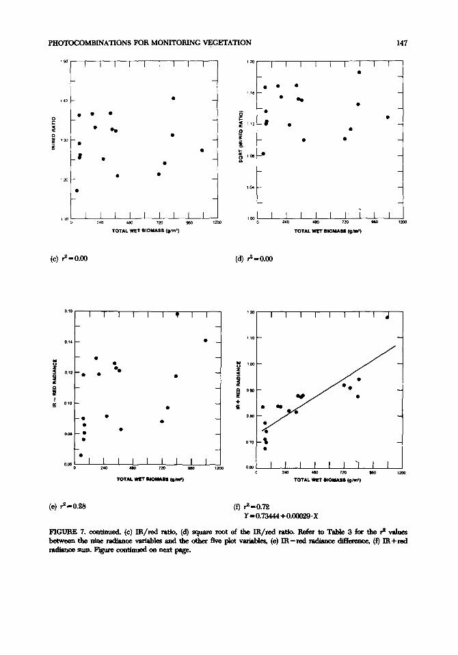
The October data demonstrated con­clusively that the various green vegeta­tion measures do not have applicability to dormant vegetation (Table 3; Fig. 7).

The use of the square-root transforma­tion for the IR/red ratio (Nalepka et al., 1977) and TV! (Rouse et aI., 1973, 1974) needs to be examined. Rouse et ai. (1973, 1974) suggest that the distribution of the VI is Poisson while Nalepka et al. (1977) suggest that the square root of IR/red ratio is more linear. The data analysis for the June data shows the same functional relationship(s) between the total wet bio­mass and IR/red ratio and square root of the IR/red ratio with the same asymp­totic nature for both plots, respectively. The asymptotic properties of the IR/red ratio, square root of the IR/red ratio, VI, and TV! are very similar as are the re­spective degrees of regression signifi­cance (Table 3; Fig. 4).

Phenological Considerations

The spectral manifestations of grass canopy phenology can be inferred from the three sampling periods used for this study. Phenological development re­sulted in the gradual accumulation of more standing vegetation in the grass canopy. By September there were ap­proximately equal amounts of standing live and dead vegetation. The October data was composed entirely of standing dead vegetation.

Spectral manifestations of grass canopy phenology can be seen by comparing the various radiance variables for the three sampling periods. The June analysis re­sults were more significant in a regression sense, showed the most nonlinearity, and

had the highest degree of intercorrelation between the six canopy variables (Tables 3 and 4). Canopy composition at this time was --80% green vegetation and only --20% dead vegetation (Table 1).

The September analysis results were less Significant in a regression sense than the June results, were linear, and had a lower degree of canopy variable intercor­relation than the June results (Tables 3 and 4). Canopy composition at this time was -52% green vegetation and -48% dead vegetation (Table 1).

The October analysis results demon­strated the need for sufficient chlorophyll absorption to occur for the IR/red ratio and related transformations to work. By this sampling time, canopy composition had simplified again and all the standing crop was standing dead vegetation. Associated with this phenolOgical condi­tion were direct linear relationships be­tween both the red and IR radiances and each of the four canopy variables sam­pled at this time. The regression results were not significant, except for three radiance variables, and there was a higher degree of canopy variable -inter­correlation than for the September data (Tables 3 and 4).

It should be noted that the "chloro­phyll" determination for the October sampling period does not present in vivo chlorophyll a and b. It is thought to represent chlorophyll decomposition products for this sampling period.

Evaluation of Different m Bandwidths

Another aspect of the study was to evaluate the influence of· IR bandwidth upon ratio technique applications for

138

(a) 0.63-0.69 I'm r=O.88

• •• • • ••• TOTAL WET BIOMASS (111m')

Y=O.I233 + 16.7980/X

5.0

o 40

~ o .. II:

$ 30

(c) r=O.86

•

•

•

520

••••

• • •

780

TOTAL WET BIOMASS (11'm')

Y = 5.5 - exp(I.6641- 0.0022· X)

•

1040 1300

C. J. TUCKER

o 7o,-----,--,---,---,---r-----,--r---,---,---

(b) 0.75-0.80 I'm r2=0.86

• •

••

••

TOTAL WET BIOMASS (111m')

Y = 0.65 - exp( -1.2680 - 0.0017· X)

"

§ i 19

o .. a:

! ... 16

~

13

•

•

• •

,0'~0-~~~~-L--5~2O~~-=780~~--,~LO-~~,300

TOTAL WET BIOMASS (111m')

(d) r=0.89 Y = 2.4 - exp(0.3926 - 0.00022 . X)

flGURE 4. The nine radiance variables plotted against the total wet biomass for the 35 plots sampled in June 1972. (a) red radiance, (b) m radiance, (c) IR/red ratio, (d) square root of the IR/red ratio. Refer to Table 3 for the r values between the nine radiance variables and the other five plot variables. Flgure continues on next pages.

PHOTOCOMBINATIONS FOR MONITORING VEGETATION 139

OJ o ~ 0.30

~ II:

a II: I 0.20

$

(e) ,.2=0.89

•

TOTAL WET BIOMASS (g/m')

¥=0.51-exp( -0.6713 -O.OO28·X)

070

060

050

>C OJ 0 ! z Q .. • ~ OJ CI OJ >

TOTAL WET BIOMASS (g/m',

(g) ,.2==0.89 ¥ = 0.70 - exp( - 0.4207 - 0.0030· X)

090

• • •

080 f-

OJ • 0 Z • " • • is • • • " • • II: 070 •• • • 0 I

OJ ••• II: • • + .. , • !!: _ . • •

060 • •

, , , ~

050~0---L--~~--l-~5~20~-L--7~8~0--l--7,'0b.40,--L~1300

TOTAL WET BIOMASS (g/m',

(f) ,.2=0.00

• •

,6

~ '2f-

I. III _

•

.. ..... . •

TOTAL WET BIOMASS (Vim',

(h) ,.2=0.94

fiGURE 4. continued. (e) IR-red radiance difference, (f) m+red radiance sum, (g) vegetation index, (h) sum/difference. Figure continued on next page.

140

OSO r r r

• • ••• • •

~ OM> - : • • • , -!! • • "

OJ • u z ••• C Ci c II: Q OJ II:

030 - •

020 I r I

0 80

1DO

• ~ 090

• 260 520 780

TOTAL WET BIOMASS (aim',

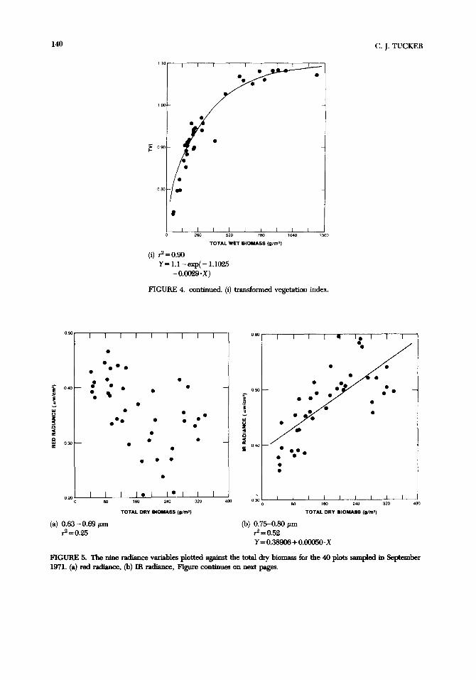
(i) ~=0.90 Y = 1.1 - exp( - 1.1025

-0.0029·X)

1040 13DO

FIGURE 4. continued. (i) transformed vegetation index.

r r I r r r 060

• • -• oso

! • • • " •• • • OJ U • • z

• C Ci

• • - c II:

040 • !!: • • • ••••

• • • • • I. I I· I I I

240 320 .DO 030 160 0 80

C. J. TUCKER

• • • • • • •

• •

240 320 400

TOTAL DRY BIOMASS (aim" TOTAL DRY BIOMASS (aim',

(a) 0.63-0.69 I'm (b) 0.75-0.80 I'm ~=0.25 r2 = 0.52

Y = 0.38906 + 0.00050' X

FIGURE 5. The nine radiance variables plotted against the total dry biomass for the 40 plots sampled in September 1971. (8) red radiance, (b) m radiance, Figure continues on next pages.

PHOTOCOMBINATIONS FOR MONITORING VEGETATION 141

3.0 170 1 I I I I I I I I I I I I I I • I I I

• • •

• 150 - • -• • 2.0 - • - •

• •• 0 • i= • •• c

0 • • II: • i= 0

~ • -. ... 1.30 ~ • • -• II: 0 • • .-. ~ ...

\.4 • i l- • , II: • • 0 •

1.0 f- ,J.. - .. • -. , • , • • 1.10 ~ -• • • •• • • • • f ..

00 I I I I I I I 0.90 1 .i .1 ..l I I I ..l 0 80 180 240 320 400 0 80 180 240 320 400

TOTAL OilY BIOMASS (Dim') TOTAL OilY BIOMASS IlI/m')

(c) r=O.32 (d) r==O.36

1.00 I I I I I I I • I I

0.40 I I I I I I I I

• • 0.95 •

0.30 I- \ - • • • • • •

0.90 l- • -• • • • ... ~

(,) • • 0.20 l- • • - z !!i S 0 0 • .. ~ 0.85 • • I· ~ • • • •

~ 0 . , • • • • ... ... IIC • 0.101- • ,

I

" • - +

! ! 0.80 l- • • • -• • • • • • •• • •• • • • • • noo f- - • • 0.75 • • • •• • • • - 0.10 I I I I I I I J 0.70 i .1 ..l .1 i .1 ..l .1 ..l

0 80 180 240 320 400 0 80 180 240 320 400

TOTAL OilY BIOMASS (O/m') TOTAL OilY IIOMASS (111m')

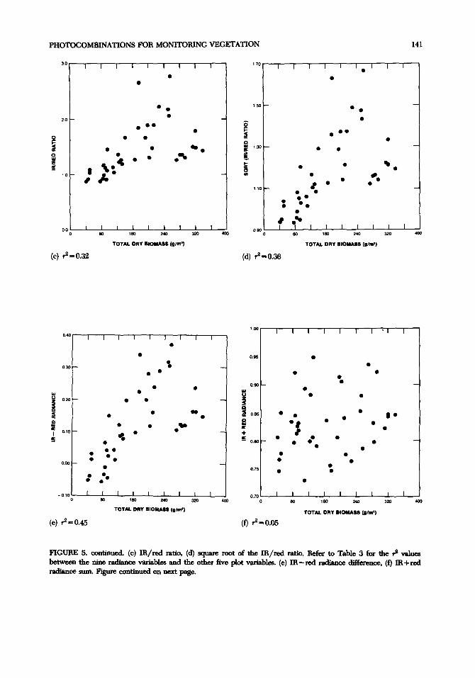
(e) r=O.45 (f) r=O.05

FIGURE 5. continued. (c) mired ratio, (d) square root of the mired ratio. Refer to Table 3 for the r values between the nine radiance variables and the other five plot variables. (e) m-red radiance difference, (f) m+red radiance SUID. Figure continued on next page.

142 C. J. TUCKER

050 100 T~~ • I I I I I

• •

040 -

• • 6(]- • -

• 030 • •• • • •

'" .. 20 f- •• -.. • • () 0 Z .. -. ! .. .. ~ ......... I!: Z 020 , .. 0 • • ... • ... ;::: i5 '" • # , •• l- i - 20 !- -.. • • :> • " •• • • tI) .. 010 > • • • • • • • • 60 - -

000 • • 100 0

I 1 1 I I I I I I

80 400 SO 16(] 240 320 400

TOTAL DRY BIOMASS (g/m') TOTAL DRY BIOMASS (g/m')

(g) ,2=0.42 (h) ,2=0.00

100 I I I I I I. I I I

• • • •

090 !- ••• -• • •

• • , •

~ OSO - • • -• • I • • • • •• • • • •

070 l- • -

• •• • •

06(] 1 I I I I I I I I 0 'so 16(] 240 320 400

TOTAL DRY BIOMASS (g/m')

(i) ,2=0.44

FlGURE 5. continued. (g) vegetation index, (h) sum/difference, (i) transfonned vegetation index.

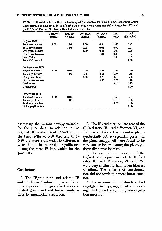
PHOTOCOMBINATIONS FOR MONITORING VEGETATION 143

TABLE 4 Correlation Mabix Between the Sampled Plot Variables for (a) 35 1/4 m2 Plots of Blue Grama

Grass Sampled in June 1972, (b) 40 1/4 m2 Plots of Blue Grama Grass Sampled in September 1971, and (c) 181/4 m2 Plots of Blue Grama Sampled in October 1972.

Total wet Total dry biomass biomass

(a) June 1972 Total wet biomass 1.00 1.00 Total dry biomass 1.00 Dry green biomass Dry brown biomass Leaf Water Total Chlorophyll

(b) September 1971 Total wet biomass 1.00 0.97 Total dry biomass 1.00 Dry green biomass Dry brown biomass Leaf water Chlorophyll

(c) October 1972 Total wet biomass 1.00 0.99 Total dry biomass 1.00 Leaf water content Chlorophyll content

estimating the various canopy variables for the June data. In addition to the original IR bandwidth of 0.75-0.80 /lm, the bandwidths of 0.80-0.90 and 0.75-0.90 /lm were evaluated. No differences were found in regression significance among the three IR bandwidths for the June data.

Conclusions

1. The IR/red ratio and related IR and red linear combinations were found to be superior to the green/red ratio and related green and red linear combina­tions for monitoring vegetation.

Dry green Dry brown Leaf Total biomass biomass water chlorophyll

1.00 0.91 1.00 0.98 0.99 0.94 0.99 0.97 1.00 0.88 1.00 0.96

1.00 0.88 0.90 1.00 0.98

1.00

0.98 0.84 0.91 0.89 0.95 0.92 0.78 0.88 1.00 0.78 0.89 0.88

1.00 0.56 0.70 1.00 0.85

1.00

0.99 0.94 0.99 0.93 1.00 0.95

1.00

2. The IR/red ratio, square root of the IR/ red ratio, IR - red difference, VI, and TVI are sensitive to the amount of photo­synthetically active vegetation present-in the plant canopy. All were found to be very similar for estimating the photosyn­thetically active biomass.

3. The asymptotic properties of the IR / red ratio, square root of the IR / red ratio, IR - red difference, VI, and TVI were very similar for high green biomass situations. The square-root transforma­tion did not result in a more linear situa­tion.

4. The accumulation of standing dead vegetation in the canopy had a lineariz­ing effect upon the various green vegeta­tion measures.

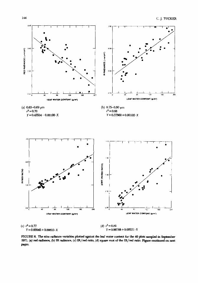
144

050,--.---,---,---r--,---,---..--.---,---,

•

• \. •• •

E 040

~ • ~ • • ,. •

• "' • • U Z c is c

' ... • • • cr 0 030 "'

• • cr

•

LEAF WATER CONTENT (g/m')

(a) 0.63-0.69!Lm r=-0.70 Y =- 0.45534 - 0.00108· X

•

• •

• • •

200

3.0 ..--...----,---,--,---,---r--,--,--,----.

• •

• 20 •

• ~ • ~ ..

LEAF WATER CONTENT (g/m')

(c) r-0.77 Y =- 0.65945 + 0.00813· X

C. J. TUCKER

060

•

• • 050

E ~ • ~

"' U z :! 0 C 040 cr !

•

• •• .­• •

• •

•

•

•

• •

• •

-• ••• •

LEAF WATER CONTENT (g/m')

(b) 0.75-0.80)Lm r2=0.68 Y =- 0.37860 + 0.00102 . X

170

150

0 ~ C cr 0 III

~ 130

0-cr 0 en

110 • • • '" • , .. ,

• ".

• • •

•

•

•• • • ,

• • •• •

LEAF WATER CONTENT (g/m2)

(d) r=0.81 Y=0.86788+0.00331·X

• : .

•

••

•

•

FIGURE 6. The nine radiance variables plotted against the leaf water content for the 40 plots sampled in September 1971. (a) red radiance, (b) IR radiance, (c) IR/red ratio, (d) square root of the IR/red ratio. Figure continued on next

pages.

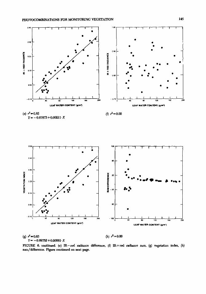
PHOTOCOMBINATIONS FOR MONITORING VEGETATION 145

0.40 '00 I I I I I I I I

• •

• • 030 • • • • • • 090 l- • -.. • • u ..

Z 020 • • u • • c z is ~ c •• • 0 • .. • : • • •• • 0 • .. • -.' 0

~ • • .. IU

I 0.10 .. • • • • +

!IE •• !IE • • • • -• 080 ~ • • • • • • • ••• • • • • 000 • • • • •••• • • • I I I I J I

- 0.10 200 • 010

80 '20 ,60 200 0 40 80 0 .0

LEAF WATER CONTENT (gIm') LEAF WATER CONTENT (g/m')

(e) r2-0.85 (f) r2"0.00 ¥= -O.07673+0.00211·X

oso '00 I I I I I I I I I

• • • 040

• 60- • -•

030 •• • .. • .. • OJ 0 • • ~ 201- • • -! III • •• z I ··.'9-- ,. •••• 0 020 , ;: ,

• ~ • • ~ I. ,. .. ~ -20 f-a •• -.. • • • ... • > 010 • • •

• • ••• -60 - -000 • , .... •

- 0 10 1 1 I I I I I I I 0 .0 60 '20 '60 200 - '00 0 40 80 '20 '60 200

LEAF WATER CONTENT (g/m') LEAF WATER CONTENT (g/m')

(g) r2=O.83 ¥= -O.09752+0.00261·X

FIGURE 6. continued. (e) IR-red radiance difference, (f) lli+red radiance sum, (g) vegetation index, (h) sum/difference. Figure continued on next page.

146

060

050

~ i . "' U 040 Z ,; • Q C a: e! Q • "' II:

• 030 •

090

~ 080

• • • • •

• • ••• 070 •

•••• • •

, •

• .. • •

.. • ,

LEAF WATER CONTENT (g/m')

(i) ,-2=0.83 Y=0.64843+0.00161·X

•

• •

• -~

i i

FIGURE 6. continued. (i) transfonned vegetation index.

070

• 0_60

j • "-

"' u Z 050 ,; 51 a: !5

040

C. J. TUCKER

•

TOTAL WET IIIOMASS (g/m') TOTAL WET IIIOMASS '81m')

(a) 0.63-0.69 p.m ,-2=0.67 Y= 0.32159 +0.00013·X

(h) 0.75-0.80 p.m ,-2=0.72 Y =0.41285+0.00017· X

FIGURE 7. The nine radiance variables plotted against the total wet biomass for the 18 plots sampled in October 1972. (a) red radiance. (h) IR radiance. Figure continued on next page.

PHOTOCOMBINATIONS FOR MONITORING VEGETATION 147

120

• • • •

"6 • 140 • .. • • • •

• ••

5' • ;:: , C 112 • a: 0

• •

130 • • ..

a: • ~ • , •

• •

.. • a: 108 a .,

• • 120

• 104

11OL-~ __ -L __ ~ __ L-~ __ ~ __ ~ __ ~~L-~ o 240 480 720 960 1200

100 0 1200

TOTAL WET BIOMASS (81m') TOTAL WIT BIOMA88 (o/m,)

(c) r==O.OO (d) r-O.OO

120

• 1.10

.. 1.00 U Z ~ 0

~ 0 090 .. a: + $

070 ,

• 1200 0.60 L-~ __ -'-__ -'-__ '--~_--"-_-'-_'----'_....J

o 240 720 960 1200

TOTAL WIT BI0MA88 (11m')

(f) r-0.72 Y -0.73444 +0.00029· X

FIGURE 7. continued. (c) IR/red ratio. (d) square root of the IR/red ratio. Refer to Table 3 for the r values between the Dine radiance variables and the other five plot variables, (e) IR-red radiance difrerence. (f) IR+red radiance sum. Figure continued on next page.

148 C. J. TUCKER

017

• • • 015

• .. " ..

110

• • • .. 0 0.13 ! •

0 Z w z

~

= • .. • • " 0.11

~

a: • w • .. 90 • .. • Q • .... • • :I ::> • III

• • • 10 • .. 009 • • •

• 007

0 1200 50

TOTAL WET IIIOMASS (g/m') TOTAL WET BIOMASS (g/m')

(h) ,-2=0.01

O.~r---r---r---~--~--'---'----r---r---r---'

0610

• • •

0800 • •• •

~ • 0,.,0

• I •

0180 •

0770 • •

0760 0 1200

TOTAL WET BIOMASS (g/m')

(i) ,-2=0.00

F1GURE 7. continued. (g) vegetation index. (h) sum/difference. (i) transfonned vegetation index.

PHOTOCOMBINATIONS FOR MONITORING VEGETATION 149

5. The regression significance for the different IR bandwidths of 0.75-0.80, 0.80-0.90, and 0.75-0.90 f.Lm were evaluated and found to be extremely sim­ilar when used with the red radiance or used in the various linear combinations.

References

Ashley, M. D., and Rea, J. (1975), Seasonal vegetation differences from ERTS im­agery, PE&RS 41, 713-719.

Blair, B. 0., and Baumgardner, M. F. (1977), Detection of the green and brown wave in hardwood canopy covers using multidate multispectral data from LANDSAT-I, Agron. ]. 69, 808-8ll.

Carneggie, D. M., deGloria, S. D., and Col­well, R N. (1974), Usefulness of ERTS-l and supporting aircraft data for monitoring plant development and range conditions in California's annual grassland, BLM Final Report 53500-CT3-266 (N).

Colwell, J. E. (1973), Bidirectional spectral reflectance of grass canopies for de­termination of above ground standing bio­mass, Ph.D. thesis, University of Michigan, University Microfilm 75-15, 693. 174 pp.

--, (1974), Vegetation canopy reflec­tance, Remote Sens. Environ. 3, 175-183.

Deering, D. W. (1978), Rangeland reflec­tance characteristics measured by aircraft and spacecraft sensors. Ph.D. dissertation. Texas A&M University, College Station, Texas, 338 pp.

Gausman, H. W., Rodriquez, R R, and Richardson, A. J. (1976), Infinite reflec­tance of dead compared with live vegeta­tion, Agron. J. 68, 295-296.

Johnson, G. R. (1976), Remote estimation of herbaceous biomass, M.S. thesis, Colorado State University, Ft. Collins, 120 pp.

Jordan, C. F. (1969), Derivation of leaf area index from quality of light on the forest floor, Ecology 50, 663-666.

Kanemasu, E. T. (1974), Seasonal canopy re­flectance patterns of wheat, sorghum, and soybean, Remote Sens. Environ. 3, 43-47.

Kauth, R J., and Thomas, G. S. (1976), The tasselled cap-a graphic description of the spectral temporal development of agricul­tural crops as seen by LANDSAT, Proceed­ings of the Symposium Machine Processing of Remote Sensing Data. LARS, Purdue.

Maxwell, E. L. (1976), Multivariate system analYSis of multispectral imagery, PE &RS 42, ll73-ll86.

Nalepka, R F., Colwell, J. E., and Rice, D. P. (1977), Forecasts of winter wheat yield and production using LANDSAT data, Fi­nal Report, NASA CR/ERIM ll4800-38-F.

Pearson, R. L., and Miller, L. D. (1972), Remote mapping of standing crop biomass for estimation of the productivity of the shortgrass prairie, Eighth International Symposium on Remote Sensing of En­vironment, University of Michigan, Ann Arbor, Mich., 1357-1381.

Pearson, R. L., Miller, L. D., and Tucker, C. J. (1976), Hand-held spectral radiometer to measure graminous biomass, Appl. Optics 15, 416-418.

Richardson, A. J., and Wiegand, C. L., (1977), Distinguishing vegetation from soil background information, PE &RS 43, 1541-1552.

Rouse, J. W., Haas, R H., Schell, J. A., and Deering, D. W. (1973), Monitoring vegeta­tion systems in the great plains with ERTS, Third ERTS Symposium, NASA SP-351 1:309-317.

Rouse, J. W, Haas, R. H., Schell, J. A., Deer­ing, D. W., and Harlan, J. C. (1974), Moni­toring the vernal advancement and retro­gradation (greenwave effect) of natural

150

vegetation. NASA/GSFC Type III Final Report, Greenbelt, Md. 371 pp.c

Salisbury, F. B., and Ross, C. (1969), Plant Physiology, Wadsworth Co., Belmont, Ca. 765 pp.

Smith, J. A., and Oliver, R. E. (1974), Effects of changing canopy directional reflectance on feature selections. Appl. Optics 13, 1599-1604.

Suits, G. R. (1972), The calculations of the directional reflectance of a vegetative canopy, Remote Sens. Environ. 2, 117-125.

Tucker, C. J. (1977a), Asymptotic nature of grass canopy spectral reflectance,. Appl. Optics 16, 1151-1157.

--, (1977b), Spectral estimation of grass

C. J. TUCKER

canopy variables, Remote Sens. Environ. 6, 11-26.

--, (1978), Postsenescent grass canopy remote sensing, Remote Sens. Environ. 7, 203-210.

Tucker, C. J., and Miller, L. D. (1977), Con­tribution of the soil spectra to grass canopy spectral reflectance, PE &RS 43, 721-726.

Tucker, C. J., and Maxwell, E. C. (1976), Sensor design for monitoring vegetation canopies, PE&RS 42, 1399-1410.

Tucker, C. J., Elgin, Jr., J. R., McMurtrey III, J. E., and Fan, C. J. (1979), Monitoring corn and soybean crop development with hand-held radiometer spectral data. Re­mote Sens. Environ. (to appear).

Received November 7, 1977; revised June 9, 1978.