recent results on the periodic lorentz gas · recent results on the periodic lorentz gas fran˘cois...

Recent Results on the Periodic Lorentz Gas

Francois Golse

To cite this version:

Francois Golse. Recent Results on the Periodic Lorentz Gas. Xavier Cabre, Juan Soler. Nonlin-ear Partial Differential Equations, Birkhauser, pp.39-99, 2012, Advanced Courses in Mathemat-ics CRM Barcelona, 978-3-0348-0190-4. <10.1007/978-3-0348-0191-1>. <hal-00390895v2>

HAL Id: hal-00390895

https://hal.archives-ouvertes.fr/hal-00390895v2

Submitted on 26 Jun 2009

HAL is a multi-disciplinary open accessarchive for the deposit and dissemination of sci-entific research documents, whether they are pub-lished or not. The documents may come fromteaching and research institutions in France orabroad, or from public or private research centers.

L’archive ouverte pluridisciplinaire HAL, estdestinee au depot et a la diffusion de documentsscientifiques de niveau recherche, publies ou non,emanant des etablissements d’enseignement et derecherche francais ou etrangers, des laboratoirespublics ou prives.

https://hal.archives-ouvertes.fr

https://hal.archives-ouvertes.fr/hal-00390895v2

RECENT RESULTS

ON THE PERIODIC LORENTZ GAS

FRANCOIS GOLSE

Abstract. The Drude-Lorentz model for the motion of electronsin a solid is a classical model in statistical mechanics, where elec-trons are represented as point particles bouncing on a fixed systemof obstacles (the atoms in the solid). Under some appropriate scal-ing assumption — known as the Boltzmann-Grad scaling by anal-ogy with the kinetic theory of rarefied gases — this system can bedescribed in some limit by a linear Boltzmann equation, assumingthat the configuration of obstacles is random [G. Gallavotti, [Phys.Rev. (2) 185 (1969), 308]). The case of a periodic configurationof obstacles (like atoms in a crystal) leads to a completely differ-ent limiting dynamics. These lecture notes review several resultson this problem obtained in the past decade as joint work with J.Bourgain, E. Caglioti and B. Wennberg.

Contents

Introduction: from particle dynamics to kinetic models 21. The Lorentz kinetic theory for electrons 42. The Lorentz gas in the Boltzmann-Grad limit

with a Poisson distribution of obstacles 73. Santalo’s formula

for the geometric mean free path 154. Estimates for the distribution of free-path lengths 215. A negative result for the Boltzmann-Grad limit

of the periodic Lorentz gas 316. Coding particle trajectories with continued fractions 357. An ergodic theorem for collision patterns 438. Explicit computation

of the transition probability P (s, h|h′) 48

2000 Mathematics Subject Classification. 82C70, 35B27 (82C40, 11A55, 11B57,11K50).

Key words and phrases. Periodic Lorentz gas, Boltzmann-Grad limit, LinearBoltzmann equation, Mean free path, Distribution of free path lengths, Continuedfractions, Farey fractions.

1

2 F. GOLSE

9. A kinetic theory in extended phase-spacefor the Boltzmann-Grad limitof the periodic Lorentz gas 55

Conclusion 59References 60

Introduction: from particle dynamics to kinetic models

The kinetic theory of gases was proposed by J. Clerk Maxwell [34, 35]and L. Boltzmann [5] in the second half of the XIXth century. Becausethe existence of atoms, on which kinetic theory rested, remained con-troversial for some time, it was not until many years later, in the XXthcentury, that the tools of kinetic theory became of common use in var-ious branches of physics such as neutron transport, radiative transfer,plasma and semiconductor physics...

Besides, the arguments which Maxwell and Boltzmann used in writ-ing what is now known as the “Boltzmann collision integral” were farfrom rigorous — at least from the mathematical viewpoint. As a matterof fact, the Boltzmann equation itself was studied by some of the mostdistinguished mathematicians of the XXth century — such as Hilbertand Carleman — before there were any serious attempt at derivingthis equation from first principles (i.e. molecular dynamics.) Whetherthe Boltzmann equation itself was viewed as a fundamental equationof gas dynamics, or as some approximate equation valid in some wellidentified limit is not very clear in the first works on the subject —including Maxwell’s and Boltzmann’s.

It seems that the first systematic discussion of the validity of theBoltzmann equation viewed as some limit of molecular dynamics —i.e. the free motion of a large number of small balls subject to binary,short range interaction, for instance elastic collisions — goes back tothe work of H. Grad [26]. In 1975, O.E. Lanford gave the first rigorousderivation [29] of the Boltzmann equation from molecular dynamics —his result proved the validity of the Boltzmann equation for a very shorttime of the order of a fraction of the reciprocal collision frequency. (Oneshould also mention an earlier, “formal derivation” by C. Cercignani[12] of the Boltzmann equation for a hard sphere gas, which consider-ably clarified the mathematical formulation of the problem.) Shortlyafter Lanford’s derivation of the Boltzmann equation, R. Illner and M.Pulvirenti managed to extend the validity of his result for all positivetimes, for initial data corresponding with a very rarefied cloud of gasmolecules [27].

PERIODIC LORENTZ GAS 3

An important assumption made in Boltzmann’s attempt at justifyingthe equation bearing his name is the “Stosszahlansatz”, to the effectthat particle pairs just about to collide are uncorrelated. Lanford’s ar-gument indirectly established the validity of Boltzmann’s assumption,at least on very short time intervals.

In applications of kinetic theory other than rarefied gas dynamics,one may face the situation where the analogue of the Boltzmann equa-tion for monatomic gases is linear, instead of quadratic. The linearBoltzmann equation is encountered for instance in neutron transport,or in some models in radiative transfer. It usually describes a situa-tion where particles interact with some background medium — suchas neutrons with the atoms of some fissile material, or photons subjectto scattering processes (Rayleigh or Thomson scattering) in a gas or aplasma.

In some situations leading to a linear Boltzmann equation, one hasto think of two families of particles: the moving particles whose phasespace density satisfies the linear Boltzmann equation, and the back-ground medium that can be viewed as a family of fixed particles ofa different type. For instance, one can think of the moving particlesas being light particles, whereas the fixed particles can be viewed asinfinitely heavier, and therefore unaffected by elastic collisions with thelight particles. Before Lanford’s fundamental paper, an important —unfortunately unpublished — preprint by G. Gallavotti [19] provideda rigorous derivation of the linear Boltzmann equation assuming thatthe background medium consists of fixed, independent like hard sphereswhose centers are distributed in the Euclidian space under Poisson’slaw. Gallavotti’s argument already possessed some of the most remark-able features in Lanford’s proof, and therefore must be regarded as anessential step in the understanding of kinetic theory.

However, Boltzmann’s Stosszahlansatz becomes questionable in thiskind of situation involving light and heavy particles, as potential cor-relations among heavy particles may influence the light particle dy-namics. Gallavotti’s assumption of a background medium consisting ofindependent hard spheres excluded this this possibility. Yet, stronglycorrelated background media are equally natural, and should also beconsidered.

The periodic Lorentz gas discussed in these notes is one example ofthis type of situation. Assuming that heavy particles are located at thevertices of some lattice in the Euclidian space clearly introduces aboutthe maximum amount of correlation between these heavy particles.This periodicity assumption entails a dramatic change in the structure

4 F. GOLSE

of the equation that one obtains under the same scaling limit thatwould otherwise lead to a linear Boltzmann equation.

Therefore, studying the periodic Lorentz gas can be viewed as oneway of testing the limits of the classical concepts of the kinetic theoryof gases.

Acknowledgements.

Most of the material presented in these lectures is the result of col-laboration with several authors: J. Bourgain, E. Caglioti, H.S. Dumas,L. Dumas and B. Wennberg, whom I wish to thank for sharing myinterest for this problem. I am also grateful to C. Boldighrini and G.Gallavotti for illuminating discussions on this subject.

1. The Lorentz kinetic theory for electrons

In the early 1900’s, P. Drude [16] and H. Lorentz [30] independentlyproposed to describe the motion of electrons in metals by the methodsof kinetic theory. One should keep in mind that the kinetic theory ofgases was by then a relatively new subject: the Boltzmann equation formonatomic gases appeared for the first time in the papers of J. ClerkMaxwell [35] and L. Boltzmann [5]. Likewise, the existence of electronshad been established shortly before, in 1897 by J.J. Thomson.

The basic assumptions made by H. Lorentz in his paper [30] can besummarized as follows.

First, the population of electrons is thought of as a gas of pointparticles described by its phase-space density f ≡ f(t, x, v), that is thedensity of electrons at the position x with velocity v at time t.

Electron-electron collisions are neglected in the physical regime con-sidered in the Lorentz kinetic model — on the contrary, in the classicalkinetic theory of gases, collisions between molecules are important asthey account for momentum and heat transfer.

However, the Lorentz kinetic theory takes into account collisionsbetween electrons and the surrounding metallic atoms. These collisionsare viewed as simple, elastic hard sphere collisions.

Since electron-electron collisions are neglected in the Lorentz model,the equation governing the electron phase-space density f is linear.This is at variance with the classical Boltzmann equation, which isquadratic because only binary collisions involving pairs of moleculesare considered in the kinetic theory of gases.

With the simple assumptions above, H. Lorentz arrived at the fol-lowing equation for the phase-space density of electrons f ≡ f(t, x, v):

(∂t + v · ∇x + 1mF (t, x) · ∇v)f(t, x, v) = Natr

2at|v|C(f)(t, x, v) .


Figure 1. Left: Paul Drude (1863-1906); right: Hen-drik Antoon Lorentz (1853-1928)

In this equation, C is the Lorentz collision integral, which acts onthe only variable v in the phase-space density f . In other words, foreach continuous function φ ≡ φ(v), one has

C(φ)(v) =

∫

|ω|=1ω·v>0

(

φ(v − 2(v · ω)ω) − φ(v))

cos(v, ω)dω ,

and the notation

C(f)(t, x, v) designates C(f(t, x, ·))(v) .The other parameters involved in the Lorentz equation are the massm of the electron, and Nat, rat respectively the density and radius ofmetallic atoms. The vector field F ≡ F (t, x) is the electric force. In theLorentz model, the self-consistent electric force — i.e. the electric forcecreated by the electrons themselves — is neglected, so that F take intoaccount the only effect of an applied electric field (if any). Roughlyspeaking, the self consistent electric field is linear in f , so that its con-tribution to the term F ·∇vf would be quadratic in f , as would be anycollision integral accounting for electron-electron collisions. Therefore,neglecting electron-electron collisions and the self-consistent electricfield are both in accordance with assuming that f ≪ 1.

6 F. GOLSE

Figure 2. The Lorentz gas: a particle path

The line of reasoning used by H. Lorentz to arrive at the kineticequations above is based on the postulate that the motion of electronsin a metal can be adequately represented by a simple mechanical model— a collisionless gas of point particles bouncing on a system of fixed,large spherical obstacles that represent the metallic atoms. Even withthe considerable simplification in this model, the argument sketched inthe article [30] is little more than a formal analogy with Boltzmann’sderivation of the equation now bearing his name.

This suggests the mathematical problem, of deriving the Lorentz ki-netic equation from a microscopic, purely mechanical particle model.Thus, we consider a gas of point particles (the electrons) moving ina system of fixed spherical obstacles (the metallic atoms). We as-sume that collisions between the electrons and the metallic atoms areperfectly elastic, so that, upon colliding with an obstacle, each pointparticle is specularly reflected on the surface of that obstacle.

Undoubtedly, the most interesting part of the Lorentz kinetic equa-tion is the collision integral which does not seem to involve F . Thereforewe henceforth assume for the sake of simplicity that there is no appliedelectric field, so that

F (t, x) ≡ 0 .

In that case, electrons are not accelerated between successive col-lisions with the metallic atoms, so that the microscopic model to beconsidered is a simple, dispersing billiard system — also called a Sinaibilliard. In that model, electrons are point particles moving at a con-stant speed along rectilinear trajectories in a system of fixed sphericalobstacles, and specularly reflected at the surface of the obstacles.

More than 100 years have elapsed since this simple mechanical modelwas proposed by P. Drude and H. Lorentz, and today we know that


the motion of electrons in a metal is a much more complicated physicalphenomenon whose description involves quantum effects.

Yet the Lorentz gas is an important object of study in nonequilibriumsatistical mechanics, and there is a very significant amount of literatureon that topic — see for instance [44] and the references therein.

The first rigorous derivation of the Lorentz kinetic equation is dueto G. Gallavotti [18, 19], who derived it from from a billiard systemconsisting of randomly (Poisson) distributed obstacles, possibly over-lapping, considered in some scaling limit — the Boltzmann-Grad limit,whose definition will be given (and discussed) below. Slightly moregeneral, random distributions of obstacles were later considered by H.Spohn in [43].

While Gallavotti’s theorem bears on the convergence of the meanelectron density (averaging over obstacle configurations), C. Boldrigh-ini, L. Bunimovich and Ya. Sinai [4] later succeeded in proving thealmost sure convergence (i.e. for a.e. obstacle configuration) of theelectron density to the solution of the Lorentz kinetic equation.

In any case, none of the results above says anything on the case of aperiodic distribution of obstacles. As we shall see, the periodic case isof a completely different nature — and leads to a very different limitingequation, involving a phase-space different from the one considered byH. Lorentz — i.e. R2 ×S1 — on which the Lorentz kinetic equation isposed.

The periodic Lorentz gas is at the origin of many challenging math-ematical problems. For instance, in the late 1970s, L. Bunimovich andYa. Sinai studied the periodic Lorentz gas in a scaling limit differentfrom the Boltzmann-Grad limit studied in the present paper. In [7],they showed that the classical Brownian motion is the limiting dynam-ics of the Lorentz gas under that scaling assumption — their work waslater extended with N. Chernov: see [8]. This result is indeed a majorachievement in nonequilibrium statistical mechanics, as it provides anexample of an irreversible dynamics (the heat equation associated withthe classical Brownian motion) that is derived from a reversible one(the Lorentz gas dynamics).

2. The Lorentz gas in the Boltzmann-Grad limitwith a Poisson distribution of obstacles

Before discussing the Boltzmann-Grad limit of the periodic Lorentzgas, we first give a brief description of Gallavotti’s result [18, 19] for thecase of a Poisson distribution of independent, and therefore possibly

8 F. GOLSE

overlapping obstacles. As we shall see, Gallavotti’s argument is in somesense fairly elementary, and yet brilliant.

First we define the notion of a Poisson distribution of obstacles.Henceforth, for the sake of simplicity, we assume a 2-dimensional set-ting.

The obstacles (metallic atoms) are disks of radius r in the Euclidianplane R2, centered at c1, c2, . . . , cj, . . . ∈ R2. Henceforth, we denote by

c = c1, c2, . . . , cj, . . . = a configuration of obstacle centers.

We further assume that the configurations of obstacle centers care distributed under Poisson’s law with parameter n, meaning that

Prob(c |#(A ∩ c) = p) = e−n|A| (n|A|)p

p!,

where |A| denotes the surface, i.e. the 2-dimensional Lebesgue measureof a measurable subset A of the Euclidian plane R2.

This prescription defines a probability on countable subsets of theEuclidian plane R2.

Obstacles may overlap: in other words, configurations c such that

for some j 6= k ∈ 1, 2, . . ., one has |ci − cj | < 2r

are not excluded. Indeed, excluding overlapping obstacles means re-jecting obstacles configurations c such that |ci − cj | ≤ 2r for somei, j ∈ N. In other words, Prob(dc) is replaced with

1

Z

∏

i>j≥0

1|ci−cj |>2rProb(dc) ,

(where Z > 0 is a normalizing coefficient.) Since the term∏

i>j≥0

1|ci−cj |>2r is not of the form∏

k≥0

φk(ck) ,

the obstacles are no longer independent under this new probabilitymeasure.

Next we define the billiard flow in a given obstacle configuration c.This definition is self-evident, and we give it for the sake of complete-ness, as well as in order to introduce the notation.

Given a countable subset c of the Euclidian plane R2, the billiardflow in the system of obstacles defined by c is the family of mappings

(X(t; ·, ·, c), V (t; ·, ·, c)) :

(

R2 \⋃

j≥1

B(cj , r)

)

× S1

defined by the following prescription.


Whenever the position X of a particle lies outside the surface of anyobstacle, that particle moves at unit speed along a rectilinear path:

X(t; x, v, c) = V (t; x, v, c) ,V (t; x, v, c) = 0 , whenever |X(t; x, v, c)− ci| > r for all i ,

and, in case of a collision with the i-th obstacle, is specularly reflectedon the surface of that obstacle at the point of impingement, meaningthat

X(t+ 0; x, v, c) = X(t− 0; x, v, c) ∈ ∂B(ci, r) ,

V (t+ 0; x, v, c) = R[

X(t; x, v, c) − cir

]

V (t− 0; x, v, c) ,

where R[ω] denotes the reflection with respect to the line (Rω)⊥:

R[ω]v = v − 2(ω · v)ω , |ω| = 1 .

Then, given an initial probability density f inc ≡ f in

c(x, v) on thesingle-particle phase-space with support outside the system of obstaclesdefined by c, we define its evolution under the billiard flow by theformula

f(t, x, v, c) = f inc(X(−t; x, v, c), V (−t; x, v, c)) , t ≥ 0 .

Let τ1(x, v, c), τ2(x, v, c), . . . , τj(x, v, c), . . . be the sequence ofcollision times for a particle starting from x in the direction −v at t = 0in the configuration of obstacles c: in other words,

τj(x, v, c) =

supt |#s ∈ [0, t] | dist(X(−s, x, v, c); c) = r = j − 1 .Denoting τ0 = 0 and ∆τk = τk − τk−1, the evolved single-particle

density f is a.e. defined by the formula

f(t, x, v, c) = f in(x− tv, v)1t<τ1

+∑

j≥1

f in

(

x−j∑

k=1

∆τkV (−τ−k )−(t− τj)V (−τ+j ), V (−τ+

j )

)

1τj<t<τj+1.

In the case of physically admissible initial data, there should be noparticle located inside an obstacle. Hence we assumed that f in

c = 0

in the union of all the disks of radius r centered at the cj ∈ c. Byconstruction, this condition is obviously preserved by the billiard flow,so that f(t, x, v, c) also vanishes whenever x belongs to a disk ofradius r centered at any cj ∈ c.

10 F. GOLSE

Figure 3. The tube corresponding with the first termin the series expansion giving the particle density

As we shall see shortly, when dealing with bounded initial data, thisconstraint disappears in the (yet undefined) Boltzmann-Grad limit, asthe volume fraction occupied by the obstacles vanishes in that limit.

Therefore, we shall henceforth neglect this difficulty and proceed asif f in were any bounded probability density on R2 × S1.

Our goal is to average the summation above in the obstacle configu-ration c under the Poisson distribution, and to identify a scaling onthe obstacle radius r and the parameter n of the Poisson distributionleading to a nontrivial limit.

The parameter n has the following important physical interpretation.The expected number of obstacle centers to be found in any measurablesubset Ω of the Euclidian plane R2 is

∑

p≥0

pProb(c |#(Ω ∩ c) = p) =∑

p≥0

pe−n|Ω| (n|Ω|)p

p!= n|Ω|

so thatn = # obstacles per unit surface in R2.

The average of the first term in the summation defining f(t, x, v, c)is

f in(x− tv, v)〈1t<τ1〉 = f in(x− tv, v)e−n2rt

(where 〈 · 〉 denotes the mathematical expectation) since the conditiont < τ1 means that the tube of width 2r and length t contains no obstaclecenter.

Henceforth, we seek a scaling limit corresponding to small obstacles,i.e. r → 0 and a large number of obstacles per unit volume, i.e. n→ ∞.


There are obviously many possible scalings satisfying this require-ment. Among all these scalings, the Boltzmann-Grad scaling in spacedimension 2 is defined by the requirement that the average over ob-stacle configurations of the first term in the series expansion for theparticle density f has a nontrivial limit.

Boltzmann-Grad scaling in space dimension 2

In order for the average of the first term above to have a nontriviallimit, one must have

r → 0+ and n→ +∞ in such a way that 2nr → σ > 0 .

Under this assumption

〈f in(x− tv, v)1t<τ1〉 → f in(x− tv, v)e−σt .

Gallavotti’s idea is that this first term corresponds with the solutionat time t of the equation

(∂t + v · ∇x)f = −nrf∫

|ω|=1ω·v>0

cos(v, ω)dω = −2nrf

f∣

∣

t=0= f in

that involves only the loss part in the Lorentz collision integral, andthat the (average over obstacle configuration of the) subsequent termsin the sum defining the particle density f should converge to theDuhamel formula for the Lorentz kinetic equation.

After this necessary preliminaries, we can state Gallavotti’s theorem.

Theorem 2.1 (Gallavotti [19]). Let f in be a continuous, bounded prob-ability density on R2 × S1, and let

fr(t, x, v, c) = f in((Xr, V r)(−t, x, v, c)) ,where (t, x, v) 7→ (Xr, V r)(t, x, v, c) is the billiard flow in the systemof disks of radius r centered at the elements of c. Assuming thatthe obstacle centers are distributed under the Poisson law of parametern = σ/2r with σ > 0, the expected single particle density

〈fr(t, x, v, ·)〉 → f(t, x, v) in L1(R2 × S1)

uniformly on compact t-sets, where f is the solution of the Lorentzkinetic equation

(∂t + v · ∇x)f + σf = σ

∫ 2π

0

f(t, x, R[β]v) sin β2

dβ4,

f∣

∣

t=0= f in ,

12 F. GOLSE

Figure 4. The tube T (t, c1, c2) corresponding with thethird term in the series expansion giving the particle den-sity

where R[β] denotes the rotation of an angle β.

End of the proof of Gallavotti’s theorem. The general term in the sum-mation giving f(t, x, v, c) is

f in

(

x−j∑

k=1

∆τkVr(−τ−k )−(t− τj)V

r(−τ+j ), V r(−τ+

j )

)

1τj<t<τj+1,

and its average under the Poisson distribution on c is

∫

f in

(

x−j∑

k=1

∆τkVr(−τ−k ) − (t− τj)V

r(−τ+j ), V r(−τ−j )

)

e−n|T (t;c1,...,cj)|njdc1 . . . dcj

j!,

where T (t; c1, . . . , cj) is the tube of width 2r around the particle tra-jectory colliding first with the obstacle centered at c1, . . . , and whosej-th collision is with the obstacle centered at cj.

As before, the surface of that tube is

|T (t; c1, . . . , cj)| = 2rt+O(r2) .

In the j-th term, change variables by expressing the positions of the jencountered obstacles in terms of free flight times and deflection angles:

(c1, . . . , cj) 7→ (τ1, . . . , τj; β1, . . . , βj) .

The volume element in the j-th integral is changed into

dc1...dcj

j!= rj sin β1

2. . . sin

βj

2dβ1

2. . .

dβj

2dτ1 . . . dτj .


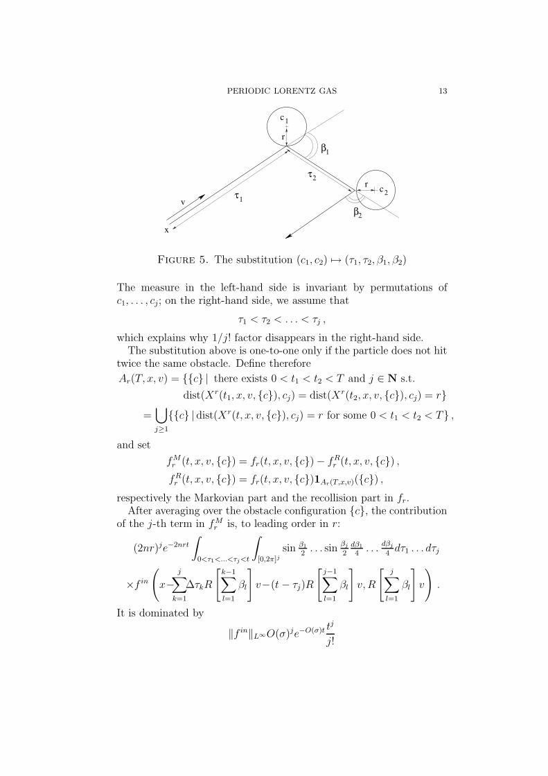
Figure 5. The substitution (c1, c2) 7→ (τ1, τ2, β1, β2)

The measure in the left-hand side is invariant by permutations ofc1, . . . , cj; on the right-hand side, we assume that

τ1 < τ2 < . . . < τj ,

which explains why 1/j! factor disappears in the right-hand side.The substitution above is one-to-one only if the particle does not hit

twice the same obstacle. Define therefore

Ar(T, x, v) = c | there exists 0 < t1 < t2 < T and j ∈ N s.t.

dist(Xr(t1, x, v, c), cj) = dist(Xr(t2, x, v, c), cj) = r=⋃

j≥1

c | dist(Xr(t, x, v, c), cj) = r for some 0 < t1 < t2 < T ,

and set

fMr (t, x, v, c) = fr(t, x, v, c) − fR

r (t, x, v, c) ,fR

r (t, x, v, c) = fr(t, x, v, c)1Ar(T,x,v)(c) ,respectively the Markovian part and the recollision part in fr.

After averaging over the obstacle configuration c, the contributionof the j-th term in fM

r is, to leading order in r:

(2nr)je−2nrt

∫

0<τ1<...<τj<t

∫

[0,2π]jsin β1

2. . . sin

βj

2dβ1

4. . .

dβj

4dτ1 . . . dτj

×f in

(

x−j∑

k=1

∆τkR

[

k−1∑

l=1

βl

]

v−(t− τj)R

[

j−1∑

l=1

βl

]

v, R

[

j∑

l=1

βl

]

v

)

.

It is dominated by

‖f in‖L∞O(σ)je−O(σ)t tj

j!

14 F. GOLSE

which is the general term of a converging series.Passing to the limit as n → +∞, r → 0 so that 2rn → σ, one finds

(by dominated convergence in the series) that

〈fMr (t, x, v, c)〉 → e−σtf in(x− tv, v)

+σe−σt

∫ t

0

∫ 2π

0

f in(x− τ1v − (t− τ1)R[β1]v, R[β1]v) sin β1

2dβ1

4dτ1

+∑

j≥2

σje−σt

∫

0<τj<...<τ1<t

∫

[0,2π]jsin β1

2. . . sin

βj

2

×f in

(

x−j∑

k=1

∆τkR

[

k−1∑

l=1

βl

]

v−(t− τj)R

[

j−1∑

l=1

βl

]

v, R

[

j∑

l=1

βl

]

v

)

×dβ1

4. . .

dβj

4dτ1 . . . dτj ,

which is the Duhamel series giving the solution of the Lorentz kineticequation.

Hence, we have proved that

〈fMr (t, x, v, ·)〉 → f(t, x, v) uniformly on bounded sets as r → 0+ ,

where f is the solution of the Lorentz kinetic equation. One can checkby a straightforward computation that the Lorentz collision integralsatisfies the property

∫

S1

C(φ)(v)dv = 0 for each φ ∈ L∞(S1) .

Integrating both sides of the Lorentz kinetic equation in the variables(t, x, v) over [0, t]×R2 ×S1 shows that the solution f of that equationsatisfies

∫∫

R2×S1

f(t, x, v)dxdv =

∫∫

R2×S1

f in(x, v)dxdv

for each t > 0.On the other hand, the billiard flow (X, V )(t, ·, ·, c) obviously leaves

the uniform measure dxdv on R2 × S1 (i.e. the particle number) in-variant, so that, for each t > 0 and each r > 0,

∫∫

R2×S1

fr(t, x, v, c)dxdv =

∫∫

R2×S1

f in(x, v)dxdv .

We therefore deduce from Fatou’s lemma that

〈fRr 〉 → 0 in L1(R2 × S1) uniformly on bounded t-sets

〈fMr 〉 → f in L1(R2 × S1) uniformly on bounded t-sets

which concludes our sketch of the proof of Gallavotti’s theorem.


For a complete proof, we refer the interested reader to [19, 20].Some remarks are in order before leaving Gallavotti’s setting for the

Lorentz gas with the Poisson distribution of obstacles.Assuming no external force field as done everywhere in the present

paper is not as inocuous as it may seem. For instance, in the case ofPoisson distributed holes — i.e. purely absorbing obstacles, so thatparticles falling into the holes disappear from the system forever —the presence of an external force may introduce memory effects in theBoltzmann-Grad limit, as observed by L. Desvillettes and V. Ricci [15].

Another remark is about the method of proof itself. One has ob-tained the Lorentz kinetic equation after having obtained an explicitformula for the solution of that equation. In other words, the equationis deduced from the solution — which is a somewhat unusual situationin mathematics. However, the same is true of Lanford’s derivation ofthe Boltzmann equation [29], as well as of the derivation of severalother models in nonequilibrium statistical mechanics. For an interest-ing comment on this issue, see [13], on p. 75.

3. Santalo’s formulafor the geometric mean free path

From now on, we shall abandon the random case and concentrateour efforts on the periodic Lorentz gas.

Our first task is to define the Boltzmann-Grad scaling for periodicsystems of spherical obstacles. In the Poisson case defined above, thingswere relatively easy: in space dimension 2, the Boltzmann-Grad scalingwas defined by the prescription that the number of obstacles per unitvolume tends to infinity while the obstacle radius tends to 0 in such away that

# obstacles per unit volume × obstacle radius → σ > 0 .

The product above has an interesting geometric meaning even with-out assuming a Poisson distribution for the obstacle centers, which weshall briefly discuss before going further in our analysis of the periodicLorentz gas.

Perhaps the most important scaling parameter in all kinetic modelsis the mean free path. This is by no means a trivial notion, as will beseen below. As suggested by the name itself, any notion of mean freepath must involve first the notion of free path length, and then someappropriate probability measure under which the free path length isaveraged.

16 F. GOLSE

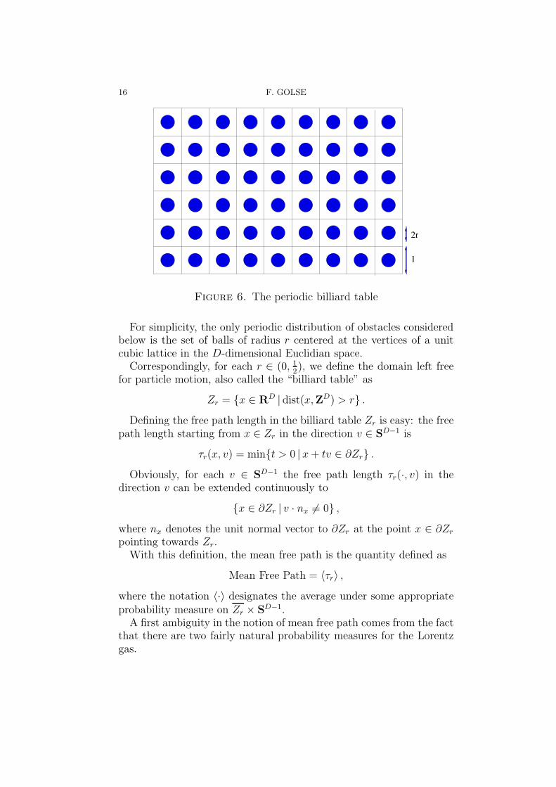
Figure 6. The periodic billiard table

For simplicity, the only periodic distribution of obstacles consideredbelow is the set of balls of radius r centered at the vertices of a unitcubic lattice in the D-dimensional Euclidian space.

Correspondingly, for each r ∈ (0, 12), we define the domain left free

for particle motion, also called the “billiard table” as

Zr = x ∈ RD | dist(x,ZD) > r .Defining the free path length in the billiard table Zr is easy: the free

path length starting from x ∈ Zr in the direction v ∈ SD−1 is

τr(x, v) = mint > 0 | x+ tv ∈ ∂Zr .Obviously, for each v ∈ SD−1 the free path length τr(·, v) in the

direction v can be extended continuously to

x ∈ ∂Zr | v · nx 6= 0 ,where nx denotes the unit normal vector to ∂Zr at the point x ∈ ∂Zr

pointing towards Zr.With this definition, the mean free path is the quantity defined as

Mean Free Path = 〈τr〉 ,where the notation 〈·〉 designates the average under some appropriateprobability measure on Zr × SD−1.

A first ambiguity in the notion of mean free path comes from the factthat there are two fairly natural probability measures for the Lorentzgas.


Figure 7. The free path length

The first one is the uniform probability measure on Zr/ZD × SD−1

dµr(x, v) =dxdv

|Zr/ZD| |SD−1|that is invariant under the billiard flow — the notation |SD−1| desig-nates the D− 1-dimensional uniform measure of the unit sphere SD−1.This measure is obviously invariant under the billiard flow

(Xr, Vr)(t, ·, ·) : Zr × SD−1 → Zr × SD−1

defined by

Xr = Vr

Vr = 0whenever X(t) /∈ ∂Zr

while

Xr(t+) = Xr(t

−) =: Xr(t) if X(t±) ∈ ∂Zr ,Vr(t

+) = R[nXr(t)]Vr(t−)

with R[n]v = v − 2v ·nn denoting the reflection with respect to thehyperplane (Rn)⊥.

The second such probability measure is the invariant measure of thebilliard map

dνr(x, v) =v ·nxdS(x)dv

v ·nxdxdv-meas(Γr+/Z

D)

where nx is the unit inward normal at x ∈ ∂Zr, while dS(x) is theD − 1-dimensional surface element on ∂Zr, and

Γr+ := (x, v) ∈ ∂Zr × SD−1 | v · nx > 0 .

The billiard map Br is the map

Γr+ ∋ (x, v) 7→ Br(x, v) := (Xr, Vr)(τr(x, v); x, v) ∈ Γr

+ ,

which obviously passes to the quotient modulo ZD-translations:

Br : Γr+/Z

D → Γr+/Z

D .

In other words, given the position x and the velocity v of a parti-cle immediatly after its first collision with an obstacle, the sequence

18 F. GOLSE

(Bnr (x, v))n≥0 is the sequence of all collision points and post-collision

velocities on that particle’s trajectory.With the material above, we can define a first, very natural notion

of mean free path, by setting

Mean Free Path = limN→+∞

1

N

N−1∑

k=0

τr(Bkr (x, v)) .

Notice that, for νr-a.e. (x, v) ∈ Γ+r /Z

D, the right hand side of theequality above is well-defined by the Birkhoff ergodic theorem. If thebilliard map Br is ergodic for the measure νr, one has

limN→+∞

1

N

N−1∑

k=0

τr(Bkr (x, v)) =

∫

Γr+/ZD

τrdνr ,

for νr-a.e. (x, v) ∈ Γr+/Z

D.Now, a very general formula for computing the right-hand side of

the above equality was found by the great spanish mathematician L.A. Santalo in 1942. In fact, Santalo’s argument applies to situationsthat are considerably more general, involving for instance curved trajec-tories instead of straight line segments, or obstacle distributions otherthan periodic. The reader interested in these questions is referred toSantalo’s original article [38].

Here is

Santalo’s formula for the geometric mean free path

One finds that

ℓr :=

∫

Γr+/ZD

τr(x, v)dνr(x, v) =1 − |BD|rD

|BD−1|rD−1

where BD is the unit ball of RD and |BD| its D-dimensional Lebesguemeasure.

In fact, one has the following slightly more general

Lemma 3.1 (H.S. Dumas, L. Dumas, F. Golse [17]). For f ∈ C1(R+)such that f(0) = 0, one has∫∫

Γr+/ZD

f(τr(x, v))v · nxdS(x)dv =

∫∫

(Zr/ZD)×SD−1

f ′(τr(x, v))dxdv .

Santalo’s formula is obtained by setting f(z) = z in the identityabove, and expressing both integrals in terms of the normalized mea-sures νr and µr.


Figure 8. Luis Antonio Santalo Sors (1911-2001)

Proof. For each (x, v) ∈ Zr × SD−1 one has

τr(x+ tv, v) = τr(x, v) − t ,

so that

d

dtτr(x+ tv, v) = −1 .

Hence τr(x, v) solves the transport equation

v · ∇xτr(x, v) = −1 , x ∈ Zr , v ∈ SD−1 ,τr(x, v) = 0 , x ∈ ∂Zr , v · nx < 0 .

Since f ∈ C1(R+) and f(0) = 0, one has

v · ∇xf(τr(x, v)) = −f ′(τr(x, v)) , x ∈ Zr , v ∈ SD−1 ,f(τr(x, v)) = 0 , x ∈ ∂Zr , v · nx < 0 .

20 F. GOLSE

Integrating both sides of the equality above, and applying Green’s for-mula shows that

−∫∫

(Zr/ZD)×SD−1

f ′(τr(x, v))dxdv

=

∫∫

(Zr/ZD)×SD−1

v · ∇x(f(τr(x, v)))dxdv

= −∫∫

(∂Zr/ZD)×SD−1

f(τr(x, v))v · nxdS(x)dv

— beware the unusual sign in the right-hand side of the second equalityabove, coming from the orientation of the unit normal nx, which ispointing towards Zr.

With the help of Santalo’s formula, we define the Boltzmann-Gradlimit for the Lorentz gas with periodic as well as random distributionof obstacles as follows:

Boltzmann-Grad scaling

The Boltzmann-Grad scaling for the periodic Lorentz gas in spacedimension D corresponds with the following choice of parameters:

distance between neighboring lattice points = ε≪ 1 ,

obstacle radius = r ≪ 1 ,

mean free path = ℓr →1

σ> 0 .

Santalo’s formula indicates that one should have

r ∼ cεD

D−1 with c =

(

σ

|BD−1|

)− 1D−1

as ε→ 0+ .

Therefore, given an initial particle density f in ∈ Cc(RD ×SD−1), we

define fr to be

fr(t, x, v) = f in

(

rD−1Xr

(

− t

rD−1;

x

rD−1, v

)

, Vr

(

− t

rD−1;x

rD−1, v

))

where (Xr, Vr) is the billiard flow in Zr with specular reflection on ∂Zr.Notice that this formula defines fr for x ∈ Zr only, as the particle

density should remain 0 for all time in the spatial domain occupied bythe obstacles. As explained in the previous section, this is a set whosemeasure vanishes in the Boltzmann-Grad limit, and we shall alwaysimplicitly extend the function fr defined above by 0 for x /∈ Zr.


Since f in is a bounded function on Zr × SD−1, the family fr de-fined above is a bounded family of L∞(RD × SD−1). By the Banach-Alaoglu theorem, this family is therefore relatively compact for theweak-* topology of L∞(R+ ×RD × SD−1).

Problem: to find an equation governing the L∞ weak-* limit pointsof the scaled number density fr as r → 0+.

In the sequel, we shall describe the answer to this question in the2-dimensional case (D = 2.)

4. Estimates for the distribution of free-path lengths

In the proof of Gallavotti’s theorem for the case of a Poisson dis-tribution of obstacles in space dimension D = 2, the probability thata strip of width 2r and length t does not meet any obstacle is e−2nrt,where n is the parameter of the Poisson distribution — i.e. the averagenumber of obstacles per unit surface.

This accounts for the loss term

f in(x− tv, v)e−σt

in the Duhamel series for the solution of the Lorentz kinetic equation,or of the term −σf on the right-hand side of that equation written inthe form

(∂t + v · ∇x)f = −σf + σ

∫ 2π

0

f(t, x, R(β)v) sin β2

dβ4.

Things are fundamentally different in the periodic case. To beginwith, there are infinite strips included in the billiard table Zr whichnever meet any obstacle.

The contribution of the 1-particle density leading to the loss termin the Lorentz kinetic equation is, in the notation of the proof ofGallavotti’s theorem

f in(x− tv, v)1t<τ1(x,v,c) .

The analogous term in the periodic case is

f in(x− tv, v)1t<rD−1τr(x/r,−v)

where τr(x, v) is the free-path length in the periodic billiard table Zr

starting from x ∈ Zr in the direction v ∈ S1.Passing to the L∞ weak-* limit as r → 0 reduces to finding

limr→0

1t<rD−1τr(x/r,−v) in w∗ − L∞(R2 × S1)

— possibly after extracting a subsequence rn ↓ 0. As we shall seebelow, this involves the distribution of τr under the probability measure

22 F. GOLSE

Figure 9. Open strips in the periodic billiard table thatnever meet any obstacle

µr introduced in the discussion of Santalo’s formula — i.e. assumingthe initial position x and direction v to be independent and uniformlydistributed on (RD/ZD) × SD−1.

We define the (scaled) distribution under µr of free path lengths τrto be

Φr(t) := µr((x, v) ∈ (Zr/ZD) × SD−1 | τr(x, v) > t/rD−1) .

Notice the scaling t 7→ t/rD−1 in this definition. In space dimensionD, Santalo’s formula shows that

∫∫

Γ+r /ZD

τr(x, v)dνr(x, v) ∼ 1|BD−1|r

1−D ,

and this suggests that the free path length τr is a quantity of the orderof 1/rD−1. (In fact, this argument is not entirely convincing, as weshall see below.)

In any case, with this definition of the distribution of free pathlengths under µr, one arrives at the following estimate.

Theorem 4.1 (Bourgain-Golse-Wennberg [6, 25]). In space dimensionD ≥ 2, there exists 0 < CD < C ′

D such that

CD

t≤ Φr(t) ≤

C ′D

twhenever t > 1 and 0 < r < 1

2.

The lower bound and the upper bound in this theorem are obtainedby very different means.


The upper bound follows from a Fourier series argument which isreminiscent of Siegel’s prood of the classical Minkowski convex bodytheorem (see [39, 36].)

The lower bound, on the other hand, is obtained by working in phys-ical space. Specifically, one uses a channel technique, introduced inde-pendently by P. Bleher [2] for the diffusive scaling.

This lower bound alone has an important consequence:

Corollary 4.2. For each r > 0, the average of the free path length(mean free path) under the probability measure µr is infinite:

∫

(Zr/ZD)×SD−1

τr(x, v)dµr(x, v) = +∞ .

Proof. Indeed, since Φr is the distribution of τr under µr, one has∫

(Zr/ZD)×SD−1

τr(x, v)dµr(x, v) =

∫ ∞

0

Φr(t)dt ≥∫ ∞

1

CD

tdt = +∞ .

Recall that the average of the free path length unded the “other”natural probability measure νr is precisely Santalo’s formula for themean free path:

ℓr =

∫∫

Γ+r /ZD

τr(x, v)dνr(x, v) =1 − |BD|rD

|BD−1|rD−1.

One might wonder why averaging the free path length τr under themeasures νr and µr actually gives two so different results.

First observe that Santalo’s formula gives the mean free path underthe probability measure νr concentrated on the surface of the obstacles,and is therefore irrelevant for particles that have not yet encounteredan obstacle.

Besides, by using the lemma that implies Santalo’s formula withf(z) = 1

2z2, one has

∫∫

(Zr/ZD)×SD−1

τr(x, v)dµr(x, v) =1

ℓr

∫

Γ+r /ZD

12τr(x, v)

2dνr(x, v) .

Whenever the components v1, . . . , vD are independent over Q, thelinear flow in the direction v is topologically transitive and ergodic onthe D-torus, so that τr(x, v) < +∞ for each r > 0 and x ∈ RD. On theother hand, τr(x, v) = +∞ for some x ∈ Zr (the periodic billiard table)whenever v belongs to some specific class of unit vectors whose compo-nents are rationally dependent, a class that becomes dense in SD−1 asr → 0+. Thus, τr is strongly oscillating (finite for irrational directions,

24 F. GOLSE

possibly infinite for a class of rational directions that becomes denseas r → 0+), and this explains why τr doesn’t have a second momentunder νr.

Proof of the Bourgain-Golse-Wennberg lower boundWe shall restrict our attention to the case of space dimension D = 2.As mentionned above, there are infinite open strips included in Zr

— i.e. never meeting any obstacle. Call a channel any such open stripof maximum width, and let Cr be the set of all channels included in Zr.

If S ∈ Cr and x ∈ S, define τS(x, v) the exit time from the channelstarting from x in the direction v, defined as

τS(x, v) = inft > 0 | x+ tv ∈ ∂S , (x, v) ∈ S × S1 .

Obviously, any particle starting from x in the channel S in the directionv must exit S before it hits an obstacle (since no obstacle intersects S).Therefore

τr(x, v) ≥ supτS(x, v) |S ∈ Cr s.t. x ∈ S ,so that

Φr(t) ≥ µr

(

⋃

S∈Cr

(x, v) ∈ (S/Z2) × S1 | τS(x, v) > t/r)

.

This observation suggests that one should carefully study the set ofchannels Cr.

Step 1: description of Cr. Given ω ∈ S1, we define

Cr(ω) := channels of direction ω in Cr ;

We begin with a lemma which describes the structure of Cr(ω).

Lemma 4.3. Let r ∈ [0, 12) and ω ∈ S1. Then

1) if S ∈ Cr(ω), then

Cr(ω) := S + k | k ∈ Z2 ;

2) if Cr(ω) 6= ∅, then

ω =(p, q)

√

p2 + q2

with

(p, q) ∈ Z2 \ (0, 0) such that g.c.d.(p, q) = 1 and√

p2 + q2 <1

2r.

We henceforth denote by Ar the set of all such ω ∈ S1. Then


Figure 10. A channel of direction ω = 1√5(2, 1); min-

imal distance d between lines L and L′ of direction ωthrough lattice points

3) for ω ∈ Ar, the elements of Cr(ω) are open strips of width

w(ω, r) =1

√

p2 + q2− 2r .

Proof of the Lemma. Statement 1) is obvious.As for statement 2), if L is an infinite line of direction ω ∈ S1 such

that ω2/ω1 is irrational, then L/Z2 is an orbit of a linear flow on T2

with irrational slope ω2/ω1. Therefore L/Z2 is dense in T2 so that Lcannot be included in Zr.

Assume that

ω =(p, q)

√

p2 + q2with (p, q) ∈ Z2 \ (0, 0) coprime,

and let L,L′ be two infinite lines with direction ω, with equations

qx− py = a and qx− py = a′ respectively.

Obviously

dist(L,L′) =|a− a′|√

p2 + q2.

If L ∪ L′ is the boundary of a channel of direction

ω = (p,q)√p2+q2

∈ A0

26 F. GOLSE

included in R2 \ Z2 — i.e. of an element of C0(ω), then L and L′

intersect Z2 so that

a, a′ ∈ pZ + qZ = Z

— the equality above following from the assumption that p and q arecoprime.

Since dist(L,L′) > 0 is minimal, then |a− a′| = 1, so that

dist(L,L′) =1

√

p2 + q2.

Likewise, if L ∪ L′ = ∂S with S ∈ Cr, then L and L′ are parallelinfinite lines tangent to ∂Zr, and the minimal distance between anysuch distinct lines is

dist(L,L′) =1

√

p2 + q2− 2r .

This entails 2) and 3).

Step 2: the exit time from a channel. Let ω = (p,q)√p2+q2

∈ Ar and let

S ∈ Cr(ω). Cut S into three parallel strips of equal width and call Sthe middle one. For each t > 1 define

θ ≡ θ(ω, r, t) := arcsin

(

rw(ω, r)

3t

)

.

Lemma 4.4. If x ∈ S and v ∈ (R[−θ]ω,R[θ]ω), where R[θ] designatesthe rotation of an angle θ, then

τS(x, v) ≥ t/r .

Moreover

µr((S/Z2) × (R[−θ]ω,R[θ]ω)) = 2

3w(ω, r)θ(ω, r, t) .

The proof of this lemma is perhaps best explained by consideringFigure 11.

Step 3: putting all channels together. Recall that we need to estimate

µr

(

⋃

S∈Cr

(x, v) ∈ (S/Z2) × S1 | τS(x, v) > t/r)

.

Pick

Ar ∋ ω = (p,q)√p2+q2

6= (p′,q′)√p′2+q′2

= ω′ ∈ Ar .


Figure 11. Exit time from the middle third S of aninfinite strip S of width w

Observe that

| sin(ω, ω′)| = |pq′−p′q|√p2+q2

√p′2+q′2

≥ 1√p2+q2

√p′2+q′2

≥ max

(

2r√p2+q2

, 2r√p′2+q′2

)

≥ sin θ(ω, r, t) + sin θ(ω′, r, t)

≥ sin(θ(ω, r, t) + θ(ω′, r, t))

whenever t > 1.Then, whenever S ∈ Cr(ω) and S ′ ∈ Cr(ω

′)

(S × (R[−θ]ω,R[θ]ω))) ∩ (S ′ × (R[θ′]ω′, R[θ′]ω′))) = ∅

with θ = θ(ω, r, t), θ′ = θ′(ω′, r, t) and R[θ] =the rotation of an angleθ.

Moreover, if ω = (p,q)√p2+q2

∈ Ar then

|S/Z2| = 13w(ω, r)

√

p2 + q2 ,

while

#S/Z2 |S ∈ Cr(ω) = 1 .

Conclusion: Therefore, whenever t > 1⋃

S∈Cr

(S/Z2) × (R[−θ]ω,R[θ]ω)

⊂⋃

S∈Cr

(x, v) ∈ (S/Z2) × S1 | τS(x, v) > t/r .

28 F. GOLSE

A channel modulo Z2

and the left-hand side is a disjoint union. Hence

µr

(

⋃

S∈Cr

(x, v) ∈ (S/Z2) × S1 | τS(x, v) > t/r)

≥∑

ω∈Ar

µr((S/Z2) × (R[−θ]ω,R[θ]ω))

=∑

g.c.d.(p,q)=1

p2+q2<1/4r2

13w(ω, r)

√

p2 + q2 · 2θ(ω, r, t)

=∑

g.c.d.(p,q)=1

p2+q2<1/4r2

23

√

p2 + q2w(ω, r) arcsin

(

rw(ω, r)

3t

)

≥∑

g.c.d.(p,q)=1

p2+q2<1/4r2

23

√

p2 + q2rw(ω, r)2

3t.

Now

√

p2 + q2 < 1/4r ⇒ w(ω, r) = 1√p2+q2

− 2r ≥ 1

2√

p2+q2,


Figure 12. Black lines issued from the origin terminateat integer points with coprime coordinates; red lines ter-minate at integer points whose coordinates are not co-prime

so that, eventually

Φr(t) ≥∑

g.c.d.(p,q)=1

p2+q2<1/16r2

23

√

p2 + q2rw(ω, r)2

3t

≥ r2

18t

∑

g.c.d.(p,q)=1

p2+q2<1/16r2

[

1

r√

p2 + q2

]

.

This gives the desired conclusion since

∑

g.c.d.(p,q)=1

p2+q2<1/16r2

[

1

4r√

p2 + q2

]

=∑

p2+q2<1/16r2

1 ∼ π

16r2.

The first equality is proved as follows: the term[

1

4r√

p2 + q2

]

is the number of integer points on the segment of length 1/4r in thedirection (p, q) with (p, q) ∈ Z2 such that g.c.d.(p, q) = 1.

30 F. GOLSE

The Bourgain-Golse-Wennberg theorem raises the question, of whe-ther Φr(t) ≃ C/t in some sense as r → 0+ and t → +∞. Given thevery different nature of the arguments used to establish the upper andthe lower bounds in that theorem, this is a highly nontrivial problem,whose answer seems to be known only in space dimension D = 2 so far.We shall return to this question later, and see that the 2-dimensionalsituation is amenable to a class of very specific techniques based oncontinued fractions, that can be used to encode particle trajectories ofthe periodic Lorentz gas.

A first answer to this question, in space dimension D = 2, is givenby the following

Theorem 4.5 (Caglioti-Golse [9]). Assume D = 2 and define, for eachv ∈ S1,

φr(t|v) = µr(x ∈ Zr/Z2 | τr(x, v) ≥ t/r , t ≥ 0 .

Then there exists Φ : R+ → R+ such that

1

| ln ε|

∫ 1/4

ε

φr(t, v)dr

r→ Φ(t) a.e. in v ∈ S1

in the limit as ε → 0+. Moreover

Φ(t) ∼ 1

π2tas t→ +∞ .

Shortly after [9] appeared, F. Boca and A. Zaharescu improved ourmethod and managed to compute Φ(t) explicitly for each t ≥ 0. Oneshould keep in mind that their formula had been conjectured earlier byP. Dahlqvist [14], on the basis of a formal computation.

Theorem 4.6 (Boca-Zaharescu [3]). For each t > 0

Φr(t) → Φ(t) =

∫ ∞

t

(s− t)g(s)ds

in the limit as r → 0+, where

g(s) = 24π2×

1 s ∈ [0, 1] ,1s

+ 2(

1 − 1s

)2ln(1 − 1

s) − 1

2

∣

∣1 − 2s

∣

∣

2ln |1 − 2

s| s ∈ (1,∞) .

In the sequel, we shall return to the continued and Farey fractionstechniques used in the proofs of these two results, and generalize them.


0.0 0.5 1.0 1.5 2.0 2.5 3.0 3.5 4.0 4.5 5.0 5.50.0

0.5

1.0

1.5

2.0

2.5

0.0 0.5 1.0 1.5 2.0 2.5 3.0 3.5 4.0 4.5 5.0 5.50.0

0.1

0.2

0.3

0.4

0.5

0.6

0.7

0.8

0.9

1.0

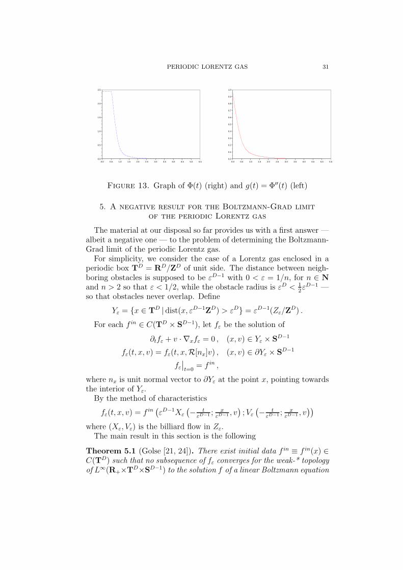
Figure 13. Graph of Φ(t) (right) and g(t) = Φ′′(t) (left)

5. A negative result for the Boltzmann-Grad limitof the periodic Lorentz gas

The material at our disposal so far provides us with a first answer —albeit a negative one — to the problem of determining the Boltzmann-Grad limit of the periodic Lorentz gas.

For simplicity, we consider the case of a Lorentz gas enclosed in aperiodic box TD = RD/ZD of unit side. The distance between neigh-boring obstacles is supposed to be εD−1 with 0 < ε = 1/n, for n ∈ N

and n > 2 so that ε < 1/2, while the obstacle radius is εD < 12εD−1 —

so that obstacles never overlap. Define

Yε = x ∈ TD | dist(x, εD−1ZD) > εD = εD−1(Zε/ZD) .

For each f in ∈ C(TD × SD−1), let fε be the solution of

∂tfε + v · ∇xfε = 0 , (x, v) ∈ Yε × SD−1

fε(t, x, v) = fε(t, x,R[nx]v) , (x, v) ∈ ∂Yε × SD−1

fε

∣

∣

t=0= f in ,

where nx is unit normal vector to ∂Yε at the point x, pointing towardsthe interior of Yε.

By the method of characteristics

fε(t, x, v) = f in(

εD−1Xε

(

− tεD−1 ;

xεD−1 , v

)

;Vε

(

− tεD−1 ;

xεD−1 , v

))

where (Xε, Vε) is the billiard flow in Zε.The main result in this section is the following

Theorem 5.1 (Golse [21, 24]). There exist initial data f in ≡ f in(x) ∈C(TD) such that no subsequence of fε converges for the weak-* topologyof L∞(R+×TD×SD−1) to the solution f of a linear Boltzmann equation

32 F. GOLSE

of the form

(∂t + v · ∇x)f(t, x, v) = σ

∫

SD−1

p(v, v′)(f(t, x, v′) − f(t, x, v))dv′

f∣

∣

t=0= f in ,

where σ > 0 and 0 ≤ p ∈ L2(SD−1 × SD−1) satisfies∫

SD−1

p(v, v′)dv′ =

∫

SD−1

p(v′, v)dv′ = 1 a.e. in v ∈ SD−1 .

This theorem has the following important — and perhaps surpris-ing — consequence: the Lorentz kinetic equation cannot govern theBoltzmann-Grad limit of the particle density in the case of a periodicdistribution of obstacles.

Proof. The proof of the negative result above involves two differentarguments:

a) the existence of a spectral gap for any linear Boltzmann equation,and

b) the lower bound for the distribution of free path lengths in theBourgain-Golse-Wennberg theorem.

Step 1: Spectral gap for the linear Boltzmann equation:With σ > 0 and p as above, consider the unbounded operator A on

L2(TD × SD−1) defined by

(Aφ)(x, v) = −v · ∇xφ(x, v) − σφ(x, v) + σ

∫

SD−1

p(v, v′)φ(x, v′)dv′ ,

with domain

D(A) = φ ∈ L2(TD × SD−1) | v · ∇xφ ∈ L2(TD × SD−1) .Then

Theorem 5.2 (Ukai-Point-Ghidouche [45]). There exists positive con-stants C and γ such that

‖etAφ− 〈φ〉‖L2(TD×SD−1) ≤ Ce−γt‖φ‖L2(TD×SD−1) , t ≥ 0 ,

for each φ ∈ L2(TD × SD−1), where

〈φ〉 = 1|SD−1|

∫∫

TD×SD−1

φ(x, v)dxdv .

Taking this theorem for granted, we proceed to the next step in theproof, leading to an explicit lower bound for the particle density.

Step 2: Comparison with the case of absorbing obstacles


Assume that f in ≡ f in(x) ≥ 0 on TD. Then

fε(t, x, v) ≥ gε(t, x, v) = f in(x− tv)1Yε(x)1εD−1τε(x/εD−1,v)>t .

Indeed, g is the density of particles with the same initial data as f , butassuming that each particle disappear when colliding with an obstacleinstead of being reflected.

Then

1Yε(x) → 1 a.e. on TD and |1Yε(x)| ≤ 1

while, after extracting a subsequence if needed,

1εD−1τε(x/εD−1,v)>t Ψ(t, v) in L∞(R+ × TD × SD−1) weak-* .

Therefore, if f is a weak-* limit point of fε in L∞(R+ × TD × SD−1)as ε → 0

f(t, x, v) ≥ f in(x− tv)Ψ(t, v) for a.e. (t, x, v) .

Step 3: using the lower bound on the distribution of τrDenoting by dv the uniform probability measure on SD−1

1|SD−1|

∫∫

TD×SD−1

f(t, x, v)2dxdv

≥ 1|SD−1|

∫∫

TD×SD−1

f in(x− tv)2Ψ(t, v)2dxdv

=

∫

TD

f in(y)2dy 1|SD−1|

∫

SD−1

Ψ(t, v)2dv

≥ ‖f in‖2L2(TD)

(

1|SD−1|

∫

SD−1

Ψ(t, v)dv

)2

= ‖f in‖2L2(TD)Φ(t)2 .

By the Bourgain-Golse-Wennberg lower bound on the distribution Φof free path lengths

‖f(t, ·, ·)‖L2(TD×SD−1) ≥CD

t‖f in‖L2(TD) , t > 1 .

On the other hand, by the spectral gap estimate, if f is a solution ofthe linear Boltzmann equation, one has

‖f(t, ·, ·)‖L2(TD×SD−1) ≤∫

TD

f in(y)dy + Ce−γt‖f in‖L2(TD)

so thatCD

t≤ ‖f in‖L1(TD)

‖f in‖L2(TD)

+ Ce−γt

for each t > 1.

34 F. GOLSE

Step 4: choice of initial dataPick ρ to be a bump function supported near x = 0 and such that

∫

ρ(x)2dx = 1 .

Take f in to be x 7→ λD/2ρ(λx) periodicized, so that∫

TD

f in(x)2dx = 1 , while

∫

TD

f in(y)dy = λ−D/2

∫

ρ(x)dx .

For such initial data, the inequality above becomes

CD

t≤ λ−D/2

∫

ρ(x)dx+ Ce−γt .

Conclude by choosing λ so that

λ−D/2

∫

ρ(x)dx < supt>1

(

CD

t− Ce−γt

)

> 0 .

Remarks:

1) The same result (with the same proof) holds for any smooth obstacleshape included in a shell

x ∈ RD |CεD < dist(x, εD−1ZD) < C ′εD .2) The same result (with same proof) holds if the specular reflectionboundary condition is replaced by more general boundary conditions,such as absorption (partial or complete) of the particles at the bound-ary of the obstacles, diffuse reflection, or any convex combination ofspecular and diffuse reflection — in the classical kinetic theory of gases,such boundary conditons are known as “accomodation boundary con-ditions”.3) But introducing even the smallest amount of stochasticity in anyperiodic configuration of obstacles can again lead to a Boltzmann-Gradlimit that is described by the Lorentz kinetic model.Example. (Wennberg-Ricci [37]) In space dimension 2, take obsta-cles that are disks of radius r centered at the vertices of the latticer1/(2−η)Z2, assuming that 0 < η < 1. Santalo’s formula suggests thatthe free-path lengths scale like rη/(2−η) → 0.

Suppose the obstacles are removed independently with large prob-ability — specifically, with probability p = 1−rη/(2−η). In that case, theLorentz kinetic equation governs the 1-particle density in the Boltzmann-Grad limit as r → 0+.

Having explained why neither the Lorentz kinetic equation nor anylinear Boltzmann equation can govern the Boltzmann-Grad limit of the


periodic Lorentz gas, in the remaining part of these notes, we build thenecessary material used in the description of that limit.

6. Coding particle trajectories with continued fractions

With the Bourgain-Golse-Wennberg lower bound for the distributionof free path lengths in the periodic Lorentz gas, we have seen that the1-particle phase space density is bounded below by a quantity that isincompatible with the spectral gap of any linear Boltzmann equation— in particular with the Lorentz kinetic equation.

In order to further analyze the Boltzmann-Grad limit of the periodicLorentz gas, we cannot content ourselves with even more refined esti-mates on the distribution of free path lengths, but we need a convenientway to encode particle trajectories.

More precisely, the two following problems must be answered some-how:

First problem: for a particle leaving the surface of an obstacle in a givendirection, to find the position of its next collision with an obstacle;

Second problem: average — in some sense to be defined — in order toeliminate the direction dependence.

From now on, our discussion is limited to the case of spatial dimen-sion D = 2, as we shall use continued fractions, a tool particularly welladapted to understanding the rational approximation of real numbers.Treating the case of a space dimension D > 2 along the same lineswould require a better understanding of simultaneous rational approx-imation of D − 1 real numbers (by D − 1 rational numbers with thesame denominator), a notoriously more difficult problem.

We first introduce some basic geometrical objects used in codingparticle trajectories.

The first such object is the notion of impact parameter.For a particle with velocity v ∈ S1 located at the position x on the

surface of an obstacle (disk of radius r), we define its impact parameterhr(x, v) by the formula

hr(x, v) = sin(nx, v) .

In other words, the absolute value of the impact parameter hr(x, v) isthe distance of the center of the obstacle to the infinite line of directionv passing through x .

Obviously

hr(x,R[nx]v) = hr(x, v)

where we recall the notation R[n]v = v − 2v · nn.

36 F. GOLSE

Figure 14. The impact parameter h correspondingwith the collision point x at the surface of an obstacle,and a direction v

Figure 15. The transfer map

The next important object in computing particle trajectories in theLorentz gas is the transfer map.

For a particle leaving the surface of an obstacle in the direction vand with impact parameter h′, define

Tr(h′, v) = (s, h) with

s = r× distance to the next collision pointh = impact parameter at the next collision

Particle trajectories in the Lorentz gas are completely determined bythe transfer map Tr and its iterates.

Therefore, a first step in finding the Boltzmann-Grad limit of theperiodic, 2-dimensional Lorentz gas, is to compute the limit of Tr asr → 0+, in some sense that will be explained later.


Figure 16. Three types of orbits: the blue orbit is theshortest, the red one is the longest, while the green oneis of the intermediate length.The black segment removedis orthogonal to the direction of the trajectories.

At first sight, this seems to be a desperately hard problem to solve,as particle trajectories in the periodic Lorentz gas depend on theirdirections and the obstacle radius in the strongest possible way. For-tunately, there is an interesting property of rational approximation onthe real line that greatly reduces the complexity of this problem.

The 3-length theorem

Question (R. Thom, 1989): on a flat 2-torus with a disk removed,consider a linear flow with irrational slope. What is the longest orbit?

Theorem 6.1 (Blank-Krikorian [1]). On a flat 2-torus with a segmentremoved, consider a linear flow with irrational slope 0 < α < 1. Theorbits of this flow have at most 3 different lengths — exceptionally 2,but generically 3. Moreover, in the generic case where these orbits haveexactly 3 different lengths, the length of the longest orbit is the sum ofthe two other lengths.

These lengths are expressed in terms of the continued fraction ex-pansion of the slope α.

38 F. GOLSE

Figure 17. The 3-term partition. The shortest orbitsare collected in the blue strip, the longest orbits in the redstrip, while the orbits of intermediate length are collectedin the green strip.

Together with E. Caglioti in [9], we proposed the idea of using theBlank-Krikorian 3-length theorem to analyze particle paths in the 2-dimensional periodic Lorentz gas.

More precisely, orbits with the same lengths in the Blank-Krikoriantheorem define a 3-term partition of the flat 2-torus into parallel strips,whose lengths and widths are computed exactly in terms of the con-tinued fraction expansion of the slope (see Figure 171.)

The collision pattern for particles leaving the surface of one obstacle— and therefore the transfer map — can be explicitly determined inthis way, for a.e. direction v ∈ S1.

In fact, there is a classical result known as the 3-length theorem,which is related to Blank-Krikorian’s. Whereas the Blank-Krikoriantheorem considers a linear flow with irrational slope on the flat 2-torus,

1Figures 16 and 17 are taken from a conference by E. Caglioti at the CentreInternational de Rencontres Mathematiques, Marseilles, February 18-22, 2008.


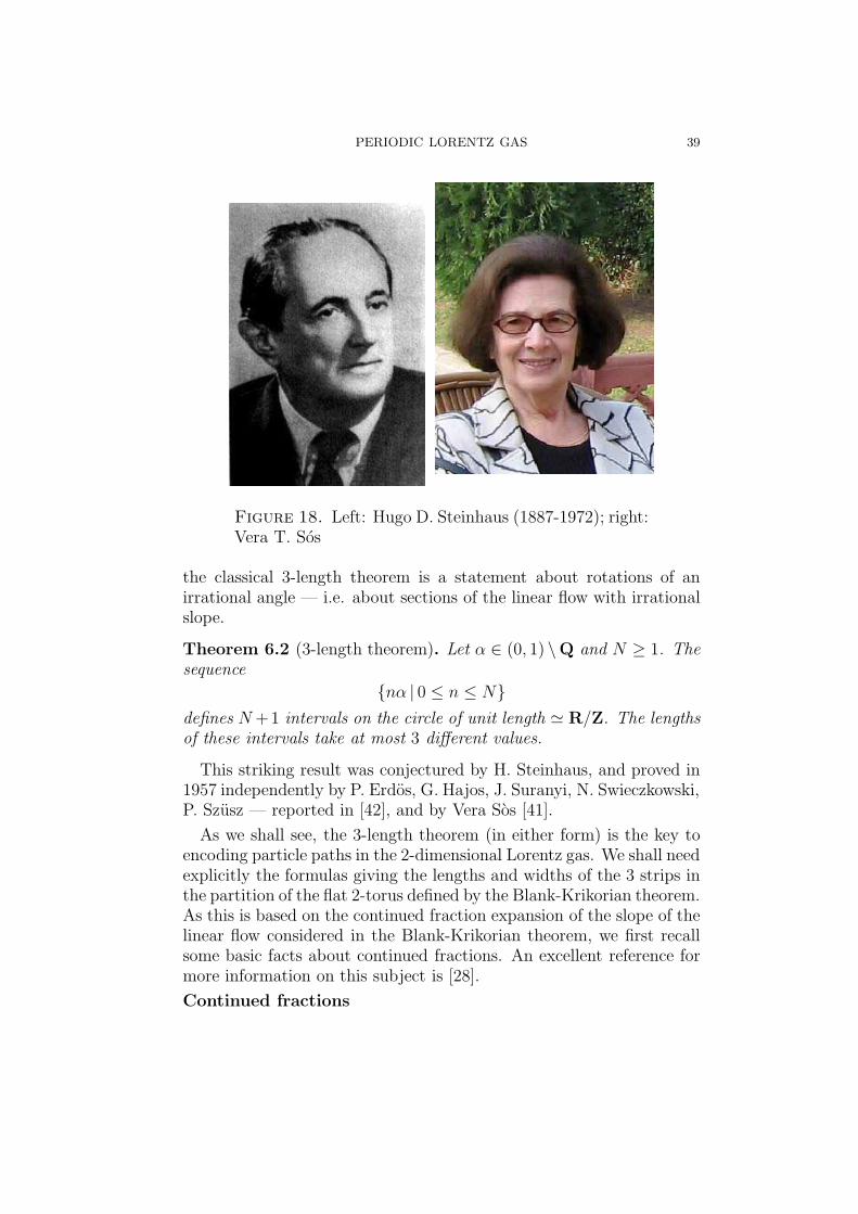
Figure 18. Left: Hugo D. Steinhaus (1887-1972); right:Vera T. Sos

the classical 3-length theorem is a statement about rotations of anirrational angle — i.e. about sections of the linear flow with irrationalslope.

Theorem 6.2 (3-length theorem). Let α ∈ (0, 1) \Q and N ≥ 1. Thesequence

nα | 0 ≤ n ≤ Ndefines N +1 intervals on the circle of unit length ≃ R/Z. The lengthsof these intervals take at most 3 different values.

This striking result was conjectured by H. Steinhaus, and proved in1957 independently by P. Erdos, G. Hajos, J. Suranyi, N. Swieczkowski,P. Szusz — reported in [42], and by Vera Sos [41].

As we shall see, the 3-length theorem (in either form) is the key toencoding particle paths in the 2-dimensional Lorentz gas. We shall needexplicitly the formulas giving the lengths and widths of the 3 strips inthe partition of the flat 2-torus defined by the Blank-Krikorian theorem.As this is based on the continued fraction expansion of the slope of thelinear flow considered in the Blank-Krikorian theorem, we first recallsome basic facts about continued fractions. An excellent reference formore information on this subject is [28].

Continued fractions

40 F. GOLSE

Assume 0 < v2 < v1 and set α = v2/v1, and consider the continuedfraction expansion of α:

α = [0; a0, a1, a2, . . .] =1

a0 +1

a1 + . . .

.

Define the sequences of convergents (pn, qn)n≥0 — meaning thatpn+2

qn+2= [0; a0, . . . , an] , n ≥ 2

— by the recursion formulas

pn+1 = anpn + pn−1 , p0 = 1 , p1 = 0 ,qn+1 = anqn + qn−1 q0 = 0 , q1 = 1 .

Finally, let dn denote the sequence of errors

dn = |qnα− pn| = (−1)n−1(qnα− pn) , n ≥ 0 ,

so thatdn+1 = −andn + dn−1 , d0 = 1 , d1 = α .

The sequence dn is decreasing and converges to 0, at least exponen-tially fast. (In fact, the irrational number for which the rational approx-imation by continued fractions is the slowest is the one for which thesequence of denominators qn have the slowest growth, i.e. the goldenmean

θ = [0; 1, 1, . . .] =1

1 +1

1 + . . .

=

√5 − 1

2.

The sequence of errors associated with θ satisfies dn+1 = −dn + dn−1

for each n ≥ 1 with d0 = 1 and d1 = θ, so that dn = θn for each n ≥ 0.)By induction, one verifies that

qndn+1 + qn+1dn = 1 , n ≥ 0 .

Notation: we write pn(α), qn(α), dn(α) to indicate the dependence ofthese quantities in α.

Collision patterns

The Blank-Krikorian 3-length theorem has the following consequence,of fundamental importance in our analysis.

Any particle leaving the surface of one obstacle in some irrationaldirection v will next collide with one of at most 3 — exceptionally 2 —other obstacles.

Any such collision pattern involving the 3 obstacles seen by the de-parting particle in the direction of its velocity is completely determinedby exactly 4 parameters, computed in terms of the continued fraction


Figure 19. Collision pattern seen from the surface ofone obstacle. Here, ε = 2r/v1.

expansion of v2/v1 — in the case where 0 < v2 < v1, to which thegeneral case can be reduced by obvious symmetry arguments.

Assume therefore 0 < v2 < v1 with α = v2/v1 /∈ Q. Henceforth, weset ε = 2r

√1 + α2 and define

N(α, ε) = infn ≥ 0 | dn(α) ≤ ε ,

k(α, ε) = −[

ε− dN(α,ε)−1(α)

dN(α,ε)(α)

]

.

The parameters defining the collision pattern are A,B,Q — as theyappear on the previous figure — together with an extra parameterΣ ∈ ±1. Here is how they are computed in terms of the continuedfraction expansion of α = v2/v1:

A(v, r) = 1 − dN(α,ε)(α)

ε,

B(v, r) = 1 − dN(α,ε)−1(α)

ε+

k(α,ε)dN(α,ε)(α)

ε,

Q(v, r) = εqN(α,ε)(α) ,

Σ(v, r) = (−1)N(α,ε) .

The extra-parameter Σ in the list above has the following geometricalmeaning. It determines the relative position of the closest and nextto closest obstacles seen from the particle leaving the surface of theobstacle at the origin in the direction v.

42 F. GOLSE

The case represented on the figure where the closest obstacle is ontop of the strip consisting of the longest particle path corresponds withΣ = +1, the case where that obstacle is at the bottom of this samestrip corresponds with Σ = −1.

The figure above showing one example of collision pattern involvesstill another parameter, denoted Q′ on that figure.

This parameter Q′ is not independent from A,B,Q, since one musthave

AQ+BQ′ + (1 − A−B)(Q+Q′) = 1

each term in this sum corresponding to the surface of one of the threestrips in the 3-term partition of the 2-torus. (Remember that the lengthof the longest orbit in the Blank-Krikorian theorem is the sum of thetwo other lengths.) Therefore

Q′(v, r) =1 −Q(v, r)(1 −B(v, r))

1 − A(v, r).

Once the structure of collision patterns elucidated with the help ofthe Blank-Krikorian variant of the 3-length theorem, we return to ouroriginal problem, namely that of computing the transfer map.

In the next proposition, we shall see that the transfer map in a given,irrational direction v ∈ S1 can be expressed explicitly in terms of theparameters A,B,Q,Σ defining the collision pattern correponding withthis direction.

DenoteK :=]0, 1[3×±1

and let (A,B,Q,Σ) ∈ K be the parameters defining the collision pat-tern seen by a particle leaving the surface of one obstacle in the direc-tion v. Set

TA,B,Q,Σ(h′) = (Q, h′ − 2Σ(1 − A))if 1 − 2A < Σh′ ≤ 1 ,

TA,B,Q,Σ(h′) = (Q′, h′ + 2Σ(1 − B))if −1 ≤ Σh′ < −1 + 2B ,

TA,B,Q,Σ(h′) = (Q′ +Q, h′ + 2Σ(A− B))if −1 + 2B ≤ Σh′ ≤ 1 − 2A .

With this notation, the transfer map is essentially given by the explicitformula TA,B,Q,Σ, except for an error of the order O(r2) on the free-pathlength from obstacle to obstacle.

Proposition 6.3 (Caglioti-Golse [10, 11]). One has

Tr(h′, v) = T(A,B,Q,Σ)(v,r)(h

′) + (O(r2), 0)

in the limit as r → 0+.


In fact, the proof of this proposition can be read on the figure abovethat represents a generic collision pattern. The first component in theexplicit formula

T(A,B,Q,Σ)(v,r)(h′)

represents exactly r× the distance between the vertical segments thatare the projections of the diameters of the 4 obstacles on the verticalordinate axis. Obviously, the free-path length from obstacle to obstacleis the distance between the corresponding vertical segments, minus aquantity of the order O(r) that is the distance from the surface of theobstacle to the corresponding vertical segment.

On the other hand, the second component in the same explicit for-mula is exact, as it relates impact parameters, which are precisely theintersections of the infinite line that contains the particle path with thevertical segments corresponding with the two obstacles joined by thisparticle path.

If we summarize what we have done so far, we see that we havesolved our first problem stated at the beginning of the present section,namely that of finding a convenient way of coding the billiard flow inthe periodic case and for space dimension 2, for a.e. given direction v.

7. An ergodic theorem for collision patterns

It remains to solve the second problem, namely, to find a conve-nient way of averaging the computation above so as to get rid of thedependence on the direction v.

Before going further in this direction, we need to recall some knownfacts about the ergodic theory of continued fractions.

The Gauss map

Consider the Gauss map, which is defined on all irrational numbersin (0, 1) as follows:

T : (0, 1) \ Q ∋ x 7→ Tx = 1x−[

1x

]

∈ (0, 1) \ Q .

This Gauss map has the following invariant probability measure —found by Gauss himself:

dg(x) = 1ln 2

dx

1 + x.

Moreover, the Gauss map T is ergodic for the invariant measuredg(x). By Birkhoff’s theorem, for each f ∈ L1(0, 1; dg)

1

N

N−1∑

k=0

f(T kx) →∫ 1

0

f(z)dg(z) a.e. in x ∈ (0, 1)

44 F. GOLSE

as N → +∞.How the Gauss map is related to continued fractions is explained as

follows: for

α = [0; a0, a1, a2, . . .] =1

a0 +1

a1 + . . .

∈ (0, 1) \ Q

the terms ak(α) of the continued fraction expansion of α can be com-puted from the iterates of the Gauss map acting on α: specifically

ak(α) =

[

1

T kα

]

, k ≥ 0

As a consequence, the Gauss map corresponds with the shift to theleft on infinite sequences of positive integers arising in the continuedfraction expansion of irrationals in (0, 1). In other words,

T [0; a0, a1, a2, . . .] = [0; a1, a2, a3 . . .] ,

equivalently recast as

an(Tα) = an+1(α) , n ≥ 0 .

Thus, the terms ak(α) of the continued fraction expansion of anyα ∈ (0, 1) \ Q are easily expressed in terms of the sequence of iter-ates (T kα)k≥0 of the Gauss map acting on α. The error dn(α) is alsoexpressed in term of that same sequence (T kα)k≥0, by equally simpleformulas.

Starting from the induction relation on the error terms

dn+1(α) = −an(α)dn(α) + dn−1(α) , d0(α) = 1 , d1(α) = α

and the explicit formula relating an(Tα) to an(α), we see that

αdn(Tα) = dn+1(α) , n ≥ 0 .

This entails the formula

dn(α) =n−1∏

k=0

T kα , n ≥ 0 .

Observe that, for each θ ∈ [0, 1] \ Q, one has

θ · Tθ < 12,

so that

dn(α) ≤ 2−[n/2] , n ≥ 0 ,


which establishes the exponential decay mentionned above. (As a mat-ter of fact, exponential convergence is the slowest possible for the con-tinued fraction algorithm, as it corresponds with the rational approx-imation of algebraic numbers of degree 2, which are the hardest toapproximate by rational numbers.)

Unfortunately, the dependence of qn(α) in α is more complicated.Yet one can find a way around this, with the following observation.Starting from the relation

qn+1(α)dn(α) + qn(α)dn+1(α) = 1 ,

we see that

qn(α)dn−1(α) =

n∑

j=1

(−1)n−j dn(α)dn−1(α)

dj(α)dj−1(α)

=

n∑

j=1

(−1)n−j

n−1∏

k=j

T k−1αT kα .

Using once more the inequality θ · Tθ < 12

for θ ∈ [0, 1] \ Q, one cantruncate the summation above at the cost of some exponentially smallerror term. Specifically, one finds that

∣

∣

∣

∣

∣

qn(α)dn−1(α) −n∑

j=n−l

(−1)n−j dn(α)dn−1(α)

dj(α)dj−1(α)

∣

∣

∣

∣

∣

=

∣

∣

∣

∣

∣

qn(α)dn−1(α) −n∑

j=n−l

(−1)n−jn−1∏

k=j

T k−1αT kα

∣

∣

∣

∣

∣

≤ 2−l .

More information on the ergodic theory of continued fractions can befound in the classical monograph [28] on continued fractions, and inSinai’s book on ergodic theory [40].

An ergodic theorem

We have seen in the previous section that the transfer map satisfies

Tr(h′, v) = T(A,B,Q,Σ)(v,r)(h

′) + (O(r2), 0) as r → 0+

for each v ∈ S1 such that v2/v1 ∈ (0, 1) \ Q.Obviously, the parameters (A,B,Q,Σ) are extremely sensitive to

variations in v and r as r → 0+, so that even the explicit formula forTA,B,Q,Σ, is not too useful in itself.

Each time one must handle a strongly oscillating quantity such asthe free path length τr(x, v) or the transfer map Tr(h

′, v), it is usuallya good idea to consider the distribution of that quantity under somenatural probability measure than the quantity itself. Following this

46 F. GOLSE

principle, we are led to consider the family of probability measures in(s, h) ∈ R+ × [−1, 1]

δ((s, h) − Tr(h′, v)) ,

or equivalentlyδ((s, h) − T(A,B,Q,Σ)(v,r)(h

′)) .

A first obvious idea would be to average out the dependence in v ofthis family of measures: as we shall see later, this is not an easy task.

A somewhat less obvious idea is to average over obstacle radius.Perhaps surprisingly, this is easier than averaging over the direction v.

That averaging over obstacle radius is a natural operation in thiscontext can be explained by the following observation. We recall thatthe sequence of errors dn(α) in the continued fraction expansion of anirrational α ∈ (0, 1) satisfies

αdn(Tα) = dn+1(α) , n ≥ 0 ,

so thatN(α, ε) = infn ≥ 1 | dn(α) ≤ ε

is transformed by the Gauss map as follows:

N(a, ε) = N(Tα, ε/α) + 1 .

In other words, the transfer map for the 2-dimensional periodicLorentz gas in the billiard table Zr (meaning, with circular obstaclesof radius r centered at the vertices of the lattice Z2) in the direction vcorresponding with the slope α is essentially the same as for the billiardtable Zr/α but in the direction corresponding with the slope Tα. Sincethe problem is invariant under the transformation

α 7→ Tα , r 7→ r/α

this suggests the idea of averaging with respect to the scale invariantmeasure in the variable r, i.e. dr

ron R∗

+.

The key result in this direction is the following ergodic lemma forfunctions that depend on finitely many dns.

Lemma 7.1 (Caglioti-Golse [9, 22, 11]). For α ∈ (0, 1) \ Q, set

N(α, ε) = infn ≥ 0 | dn(α) ≤ ε .For each m ≥ 0 and each f ∈ C(Rm+1

+ ), one has

1

| ln η|

∫ 1/4

η

f

(

dN(α,ε)(α)

ε, . . . ,

dN(α,ε)−m(α)

ε

)

dε

ε→ Lm(f)

a.e. in α ∈ (0, 1) as η → 0+, where the limit Lm(f) is independent ofα.


With this lemma, we can average over obstacle radius any functionthat depends on collision patterns, i.e. any function of the parametersA,B,Q,Σ.

Proposition 7.2 (Caglioti-Golse [11]). Let K = [0, 1]3 × ±1. Foreach F ∈ C(K), there exists L(F ) ∈ R independent of v such that

1

ln(1/η)

∫ 1/2

η

F (A(v, r), B(v, r), Q(v, r),Σ(v, r))dr

r→ L(F )

for a.e. v ∈ S1 such that 0 < v2 < v1 in the limit as η → 0+.

Sketch of the proof. First eliminate the Σ dependence by decomposing

F (A,B,Q,Σ) = F+(A,B,Q) + ΣF−(A,B,Q) .

Hence it suffices to consider the case where F ≡ F (A,B,Q).Setting α = v2/v1 and ε = 2r/v1, we recall that

A(v, r) is a function ofdN(α,ε)(α)

ε,

B(v, r) is a function ofdN(α,ε)(α)

εand

dN(α,ε)−1(α)

ε.

As for the dependence of F on Q, proceed as follows: in F (A,B,Q),replace Q(v, r) with

ε

dN(α,ε)−1

N(α,ε)∑

j=N(α,ε)−l

(−1)N(α,ε)−j dN(α,ε)(α)dN(α,ε)−1(α)

dj(α)dj−1(α),

at the expense of an error term of the order

O(modulus of continuity of F (2−m)) → 0 as l → 0 ,

uniformly as ε→ 0+.This substitution leads to an integrand of the form

f

(

dN(α,ε)(α)

ε, . . . ,

dN(α,ε)−m−1(α)

ε

)

to which we apply the ergodic lemma above: its Cesaro mean converges,in the small radius limit, to some limit Lm(F ) independent of α.

By uniform continuity of F , one finds that

|Lm(F ) − Lm′(F )| = O(modulus of continuity of F (2−m∨m′

))

(with the notation m ∨m′ = max(v, v′)), so that Lm(F ) is a Cauchysequence as m→ ∞. Hence

Lm(F ) → L(F ) as m→ ∞

48 F. GOLSE

and with the error estimate above for the integrand, one finds that

1

ln(1/η)

∫ 1/2

η


r→ L(F )

as η → 0+.

With the ergodic theorem above, and the explicit approximation ofthe transfer map expressed in terms of the parameters (A,B,Q,Σ)that determine collision patterns in any given direction v, we easilyarrive at the following notion of a “probability of transition” for aparticle leaving the surface of an obstacle with an impact parameter h′

to hit the next obstacle on its trajectory at time s/r with an impactparameter h.

Theorem 7.3 (Caglioti-Golse, [10, 11]). For each h′ ∈ [−1, 1], thereexists a probability density P (s, h|h′) on R+ × [−1, 1] such that, foreach f ∈ C(R+ × [−1, 1]),

1

| ln η|

∫ 1/4

η

f(Tr(h′, v))

dr

r→∫ ∞

0

∫ 1

−1

f(s, h)P (s, h|h′)dsdh

a.e. in v ∈ S1 as η → 0+.

In other words, the transfer map converges in distribution and in thesense of Cesaro, in the small radius limit, to a transition probabilityP (s, h|h′) that is independent of v.

We are therefore left with the following problems:a) to compute the transition probability P (s, h|h′) explicitly and dis-cuss its properties, andb) to explain the role of this transition probability in the Boltzmann-Grad limit of the periodic Lorentz gas dynamics.

8. Explicit computationof the transition probability P (s, h|h′)

Most unfortunately, our argument leading to the existence of thelimit L(F ), the core result of the previous section, cannot be used forcomputing explicitly the value L(F ). Indeed, the convergence proof isbased on the ergodic lemma in the last section, coupled to a sequenceof approximations of the parameter Q in collision patterns that involveonly finitely many error terms dn(α) in the continued fraction expansionof α. The existence of the limit is obtained through Cauchy’s criterion,precisely because of the difficulty in finding an explicit expression forthe limit.


Nevertheless, we have arrived at the following expression for thetransition probability P (s, h|h′):Theorem 8.1 (Caglioti-Golse [10, 11]). The transition probability den-sity P (s, h|h′) is expressed in terms of a = 1

2|h− h′| and b = 1

2|h + h′|

by the explicit formula

P (s, h|h′) =3

π2sa

[

(

(s− 12sa)∧(1 + 1

2sa)−(1∨(1

2s + 1

2sb))

+

+(

(s− 12sa)∧1−((1

2s+ 1

2sb)∨

(

1− 12sa))

+

+sa∧|1 − s|1s<1 + (sa−|1 − s|)+

]

,

with the notations x ∧ y = min(x, y) and x ∨ y = max(x, y).Moreover, the function

(s, h, h′) 7→ (1 + s)P (s, h|h′) belongs to L2(R+ × [−1, 1]2) .

In fact, the key result in the proof of this theorem is the asymptoticdistribution of 3-obstacle collision patterns — i.e. the computation ofthe limit L(f), whose existence has been proved in the last section’sproposition.

Theorem 8.2 (Caglioti-Golse [11]). Define K = [0, 1]3 × ±1; then,for each F ∈ C(K)

1

| ln η|

∫ 1/4

η

F ((A,B,Q,Σ)(v, r))dr

r→ L(F )

=

∫

K

F (A,B,Q,Σ)dm(A,B,Q,Σ) a.e. in v ∈ S1

as η → 0+, where

dm(A,B,Q,Σ) = dm0(A,B,Q) ⊗ 12(δΣ=1 + δΣ=−1) ,

dm0(A,B,Q) = 12π2 10<A<110<B<1−A10<Q< 1

2−A−B

dAdBdQ

1 − A.

Before giving an idea of the proof of the theorem above on the dis-tribution of 3-obstacle collision patterns, it is perhaps worthwhile ex-plaining why the measure m above is somehow natural in the presentcontext.

To begin with, the constraints 0 < A < 1 and 0 < B < 1 − A havean obvious geometric meaning (see figure 18 on collision patterns.)More precisely, the widths of the three strips in the 3-term partitionof the 2-torus minus the slit constructed in the penultimate section (asa consequence of the Blank-Krikorian 3-length theorem) add up to 1.Since A is the width of the strip consisting of the shortest orbits in

50 F. GOLSE

the Blank-Krikorian theorem, and B that of the strip consisting of thenext to shortest orbits, one has

0 < A+B ≤ 1

with equality only in the exceptional case where the orbits have atmost 2 different lengths, which occurs for a set of measure 0 in v or r.Therefore, one has

0 < B(v, r) < 1 −A(v, r) , for a.e. r ∈ (0, 12) .

Likewise, the total area of the 2-torus is the sum of the areas of thestrips consisting of all orbits with the 3 possible lengths:

1 = QA+Q′B + (Q+Q′)(1 − A−B) = Q(1 −B) +Q′(1 − A)

≥ Q(2 − A− B)

as Q′ ≥ Q (see again the figure above on collision patterns.)Therefore, the volume element

dAdBdQ

1 − A

in the expression of dm0 imples that the parameters A, B1−A

— orequivalently B mod. 1 − A — and Q are independent and uniformlydistributed in the largest subdomain of [0, 1]3 that is compatible withthe geometric constraints.

The first theorem is a consequence of the second: indeed, P (s, h|h′)dsdhis the image measure of dm(A,B,Q,Σ) under the map

K ∋ (A,B,Q,Σ) 7→ T(A,B,Q,Σ)(h′, v) .

That (1 + s)P (s, h|h′) is square integrable is proved by inspection —by using the explicit formula for P (s, h|h′).

Therefore, it remains to prove the second theorem.We are first going to show that the family of averages over velocities

satisfy∫

|v|=10<v2<v1

F (A(v, r), B(v, r), Q(v, r),Σ(v, r))dv

→ π8

∫

K

F (A,B,Q,Σ)dm(A,B,Q,Σ)

as r → 0+ for each F ∈ Cb(K).On the other hand, because of the proposition in the previous section

1

ln(1/η)

∫ 1/2

η


r→ L(F )

for a.e. v ∈ S1 such that 0 < v2 < v1 in the limit as η → 0+.


Since we know that the limit L(F ) is independent of v, comparingthe two convergence statements above shows that

L(F ) =

∫

K

F (A,B,Q,Σ)dm(A,B,Q,Σ) .

Therefore, we are left with the task of computing

limr→0+

∫

|v|=10<v2<v1

F (A(v, r), B(v, r), Q(v, r),Σ(v, r))dv .

The method for computing this type of expression is based ona) Farey fractions (sometimes called “slow continued fractions”), andb) estimates for Kloosterman’s sums, due to Boca-Zaharescu [3].To begin with, we need to recall a few basic facts about Farey frac-

tions.

Farey fractions

Put a filtration on the set of rationals in [0, 1] as follows

FQ = pq| 0 ≤ p ≤ q ≤ Q , g.c.d.(p, q) = 1

indexed in increasing order:

0 =0

1< γ1 < . . . < γj =

pj

qj< . . . < γϕ(Q) =

1

1= 1

where ϕ denotes Euler’s totient function:

φ(n) = n∏

p primep|n

(

1 − 1

p

)

.

An important operation in the construction of Farey fractions is thenotion of “mediant” of two fractions. Given two rationals

γ =p

qand γ =

p

q

with

0 ≤ p ≤ q , 0 ≤ p ≤ q , and g.c.d.(p, q) = g.c.d.(p, q) = 1 ,

their mediant is defined as

mediant = γ ⊕ γ :=p+ p

q + q∈ (γ, γ) .

Hence, if γ = pq< γ = p

qadjacent in FQ, then

aq − aq = 1 and q + q > Q .

Conversely, q, q are denominators of adjacent fractions in FQ if andonly if

0 ≤ q, q ≤ Q , q + q > Q , g.c.d.(q, q′) = 1 .

52 F. GOLSE

Figure 20. The Stern-Brocot tree. Each fraction γ onthe n-th line is the mediant of the two fractions closestto γ on the n− 1-st line. The first line consists of 0 and1 written as 0 = 0

1and 1 = 1

1. Each rational in [0, 1] is

obtained in this way.

Given α ∈ (0, 1)\Q and Q ≥ 1, there exists a unique pair of adjacentFarey fractions in FQ, henceforth denoted γ(α,Q) and γ(α,Q), suchthat

γ(α,Q) =p(α,Q)

q(α,Q)< α < γ(α,Q) =

p(α,Q)

q(α,Q).

At this point, we recall the relation between Farey and continuedfractions.

Pick 0 < ε < 1; we recall that, for each α ∈ (0, 1) \ Q,

N(α, ε) = minn ∈ N | dn(α) ≤ ε , dn(α) = dist(qn(α)α,Z) .

Set Q = [1/ε], and let

γ(α,Q) =p(α,Q))

q(α,Q)< γ(α,Q) =

p(α,Q))

q(α,Q)

with g.c.d.(p(α,Q)), q(α,Q)) = g.c.d.(p(α,Q)), q(α,Q)) = 1 be the twoadjacent Farey fractions in FQ surrounding α. Then

a) one of the two integers q(α,Q) and q(α,Q) is the denominator ofthe N(α, ε)-th convergent in the continued fraction expansion of α, i.e.qN(α,ε)(α), and


b) the other is of the form

mqN(α,ε) + qN(α,ε)−1 , with 0 ≤ m ≤ aN(α,ε)(α) ,

where we recall that

α = [0; a1, a2, . . .] =1

a0 +1

a1 + . . .

.

Setting α = v2/v1 and ε = 2r/v1, we recall that, by definition

Q(v, r) = εqN(α,ε)(α) ∈ εq(α,Q), εq(α,Q) with Q = [1/ε] ,

and we further define

D(v, r) = dN(α,ε)/ε = dist(1εQ(v, r)α,Z)/ε ,

andQ(v, r) = εq(α,Q) if qN(α,ε)(α) = q(α,Q) ,

Q(v, r) = εq(α,Q) if qN(α,ε)(α) = q(α,Q) .

Now, we recall that A(v, r) = 1 −D(v, r); moreover, we see that

B(v, r) = 1 − dN(α,ε)−1(α)

ε−[

1 − dN(α,ε)−1(α)/ε

D(v, r)

]

D(v, r)

= 1 − dN(α,ε)−1(α)/ε mod. D(v, r)

= 1 − dist(1εQ(v, r)α,Z)/ε mod. D(v, r) .

To summarize, we have

F (A(v, r), B(v, r), Q(v, r)) = G(Q(v, r), Q(v, r), D(v, r))

and we are left with the task of computing

limr→0+

∫

S1+

G(Q(v, r), Q(v, r), D(v, r))dv

where S1+ is the first octant in the unit circle. The other octants in the

unit circle give the same contribution by obvious symmetry arguments.More specifically:

Lemma 8.3. Let α ∈ (0, 1) \Q, and let pq< α < p

qbe the two adjacent

Farey fractions in FQ surrounding α, with Q = [1/ε]. Thena) if p

q< α ≤ p−ε

q, then

Q(v, r) = εq , Q(v, r) = εq , D(v, r) = 1ε(αq − p) ;

54 F. GOLSE

b) if p+εq< α < p

q, then

Q(v, r) = εq , Q(v, r) = εq , D(v, r) = 1ε(p− αq) ;

c) if p+εq< α ≤ p−ε

q, then

Q(v, r) = ε(q∧ q) , Q(v, r) = ε(q∨ q) , D(v, r) = dist(1εQ(v, r)α,Z) .

Therefore, assuming for simplicity that

G(x, y, z) = g(x, y)H ′(z) and ε = 1/Q ,

one has∫

S1+

G(Q(v, r), Q(v, r), D(v, r))dv

=∑

0<q,q≤Q<q+qg.c.d.(q,q)=1

∫ (p−ε)/q

p/q

g

(

q

Q ,q

Q

)

H ′(Q(qα− p))dα

+ three other similar terms

=∑


g

(

q

Q ,q

Q

)

1

qQ

(

H

(

1 − q/Qq/Q

)

−H(0)

)

+ three other similar terms.

Then, everything reduces to computing

limQ→+∞

1

Q2

∑


ψ

(

q

Q ,q

Q

)

.

We conclude with the following

Lemma 8.4 (Boca-Zaharescu [3]). For ψ ∈ Cc(R2), one has

1

Q2

∑


ψ

(

q

Q ,q

Q

)

→ 6π2

∫∫

0<x,y<1<x+y

ψ(x, y)dxdy

in the limit as Q → ∞.

This is precisely the path followed by F. Boca and A. Zaharescu tocompute the limiting distribution of free path lengths in [3] (see Theo-rem 4.6); as explained above, their analysis can be greatly generalizedin order to compute the transition probability that is the limit of thetransfer map as the obstacle radius r → 0+.


9. A kinetic theory in extended phase-spacefor the Boltzmann-Grad limitof the periodic Lorentz gas

We are now ready to propose an equation for the Boltzmann-Gradlimit of the periodic Lorentz gas in space dimension 2. For each r ∈]0, 1

2[, denote

Br : Γ+r ∋ (x, v) 7→ Br(x, v) = (x+ τr(x, v)v,R[x+ τr(x, v)v]v) ∈ Γ+

r

the billiard map. For (x0, v0) ∈ Γ+r , set

(xn, vn) = Bnr (x0, v0)

and define

bnr (x, v) = (A,B,Q,Σ)(vn, r) , n ∈ N∗ .

Henceforth, for each n ≥ 1, we denote

Kn := R2 × S1 × R+ × [−1, 1] × Kn .

We make the following asymptotic independence hypothesis: thereexists a probability measure Π on R+×[−1, 1] such that, for each n ≥ 1and each Ψ ∈ C(Kn) with compact support

(H)

limr→0+

∫

Zr×S1

Ψ(x, v, rτr(xr, v), hr(

x1

r, v1), b

1r, . . . , b

nr )dxdv

=

∫

Qn

Ψ(x, v, τ, h, β1, . . . , βn)dxdvdΠ(τ, h)dm(β1) . . . dm(βn) ,

where

(x0, v0) = (x− τr(x,−v)v, v) , and hr(x1

r, v1) = sin(nx1, v1)

and m is the probability measure on K obtained in Theorem 8.2.If this holds, the iterates of the transfer map Tr are described by the

Markov chain with transition probability P (s, h|h′).This leads to a kinetic equation on an extended phase space for the

Boltzmann-Grad limit of the periodic Lorentz gas in space dimension2:F (t, x, v, s, h) =

density of particles with velocity v and position x at time t

that will hit an obstacle after time s, with impact parameter h.

Theorem 9.1 (Caglioti-Golse [10, 11]). Assume (H), and let f in ≥ 0belong to Cc(R

2 × S1). Then one has

fr →∫ ∞

0

∫ 1

−1

F (·, ·, ·, s, h)dsdh in L∞(R+ ×R2 × S1) weak-∗

56 F. GOLSE

in the limit as r → 0+, where F ≡ F (t, x, v, s, h) is the solution of

(∂t+v · ∇x − ∂s)F (t, x, v, s, h)

=

∫ 1

−1

P (s, h|h′)F (t, x, R[π − 2 arcsin(h′)]v, 0, h′)dh′ ,

F (0, x, v, s, h) = f in(x, v)

∫ ∞

s

∫ 1

−1

P (τ, h|h′)dh′dτ ,

with (x, v, s, h) running through R2 × S1 ×R∗+×]− 1, 1[. The notation

R[θ] designates the rotation of an angle θ.

Let us briefly sketch the computation leading to the kinetic equationabove in the extended phase space Z = R2 × S1 ×R+ × [−1, 1].

In the limit as r → 0+, the sequence (bnr (x, v))n≥1 converges to asequence of i.i.d. random variables with values in K = [0, 1] × ±1,according to assumption (H).

Then, for each s0 > 0 and h0 ∈ [−1, 1], we construct a Markov chain(sn, hn)n≥1 with values in R+ × [−1, 1] in the following manner:

(sn, hn) = Tbn(hn−1) , n ≥ 1 .

Now we define the jump process (Xt, Vt, St, Ht) starting from (x, v, s, h)in the following manner.

First pick a trajectory of the sequence b = (bn)n≥1; then, for eachs > 0 and each h ∈ [−1, 1], set

(s0, h0) = (s, h) .

Define then inductively sn and hn for n ≥ 1 by the formula above,together with

σn = s0 + . . .+ sn−1 , n ≥ 1 ,

and

vn = R[2 arcsin(hn−1) − π]vn−1 , n ≥ 1 .

With the sequence (vn, sn, hn)n≥1 so defined, we next introduce theformulas for (Xt, Vt, St, Ht):

• While 0 ≤ t < τ , we set

Xt(x, v, s, h) = x+ tω , St(x, v, s, h) = s− t ,

Vt(x, v, s, h) = v , Ht(x, v, s, h) = h .


• For σn < t < σn+1, we set

Xt(x, v, s, h) = x+ (t− σn)vn ,

Vt(x, v, s, h) = vn ,

Tt(x, v, s, h) = σn+1 − t ,

Ht(x, v, s, h) = hn .

To summarize, the prescription above defines, for each t ≥ 0, a mapdenoted Tt:

Z × KN∗ ∋ (x, v, s, h,b) 7→ Tt(x, ω, τ, h) = (Xt, Vt, St, Ht) ∈ Z

that is piecewise continuous in t ∈ R+.Denote by f in ≡ f in(x, v, s, h) the initial distribution function in

the extended phase space Z, and by χ ≡ χ(x, v, s, h) an observable —without loss of generality, we assume that χ ∈ C∞

c (Z).Define f(t, ·, ·, ·, ·) by the formula∫∫∫∫

Z

χ(x, v, s, h)f(t, dx, dv, ds, dh)

=

∫∫∫∫

Z

E[χ(Tt(x, v, s, h)))]fin(x, ω, τ, h)dxdvdsdh ,

where E designates the expectation on trajectories of the sequence ofi.i.d. random variables b = (bn)n≥1.

In other words, f(t, ·, ·, ·, ·) is the image under the map Tt of themeasure Prob(db)f in(x, ω, τ, h), where

Prob(db) =∏

n≥1

dm(bn) .

Set g(t, x, v, s, h) = E[χ(Tt(x, v, s, h)))]; one has

g(t, x, v, s, h) = E[1t<sχ(Tt(x, v, s, h)))] + E[1s<tχ(Tt(x, v, s, h)))] .

If s > t, there is no collision in the time interval [0, t] for the trajectoryconsidered, meaning that

Tt(x, v, s, h) = (x+ tv, v, s− t, h) .

Hence

E[1t<sχ(Tt(x, v, s, h)))] = χ(x+ tv, v, s− t, h)1t<s .

On the other hand

E[1s<tχ(Tt(x, v, s, h))] = E[1s<tχ(T(t−s)−0Ts+0(x, v, s, h))]

= E[1s<tχ(T(t−s)−0(x+ sv,R[∆(h)]v, s1, h1))]

with (s1, h1) = Tb1(h) and ∆(h) = 2 arcsin(h) − π.

58 F. GOLSE

Conditioning with respect to (s1, h1) shows that

E[1s<tχ(Tt(x, v, s, h)))]

= E[1s<tE[χ(T(t−s)−0(x+ sv,R[∆(h)]v, s1, h1))|s1, h1]] ,

andE[χ(T(t−s)−0(x+ sv,R[∆(h)]v, s1, h1))|s1, h1]

= g(t− s, x+ sv,R[∆(h)]v, s1, h1) .

Then

E[1s<tE[χ(T(t−s)−0(x+ sv,R[∆(h)]v, s1, h1))|s1, h1]]

= 1s<t

∫

g(t− s, x+ sv,R[∆(h)]v,Tb1(h))]dm(b1)

= 1s<t

∫

g(t− s, x+ sv,R[∆(h)]v, s1, h1)]P (s1, h1|h)ds1dh1 .

Finally

g(t, x, v, s, h) = χ(x+ tv, v, s− t, h)1t<s

+ 1s<t

∫

g(t− s, x+ sv,R[∆(h)]v, s1, h1)]P (s1, h1|h)ds1dh1 .

This formula represents the solution of the problem

(∂t − v · ∇x + ∂s)g = 0 , t, s > 0 , x ∈ R2 , s ∈ S1 , |h| < 1

g(t, x, s, 0, h) =

∫∫

R∗+×]−1,1[

P (s1, h1|h)g(t, x, v, s1, h1)ds1dh1 ,

g∣

∣

t=0= χ .

The boundary condition for s = 0 can be replaced with a source termthat is proportional to the Dirac measure δs=0:

(∂t − v · ∇x + ∂s)g = δs=0

∫∫

R∗+×]−1,1[

P (s1, h1|h)g(t, x, v, s1, h1)ds1dh1 ,

g∣

∣

t=0= χ .

One concludes by observing that this problem is precisely the adjointof the Cauchy problem in the theorem.

Let us conclude this section with a few bibliographical remarks.Although the Boltzmann-Grad limit of the periodic Lorentz gas is a

fairly natural problem, it remained open for quite a long time after thepioneering work of G. Gallavotti on the case of a Poisson distributionof obstacles [18, 19].

Perhaps the main conceptual difficulty was to realize that this limitmust involve a phase-space other than the usual phase-space of kinetic


theory, i.e. the set R2 × S1 of particle positions and velocities, and tofind the appropriate extended phase-space where the Boltzmann-Gradlimit of the periodic Lorentz gas can be described by an autonomousequation.

Already Theorem 5.1 in [9] suggested that, even in the simplest prob-lem where the obstacles are absorbing — i.e. holes where particlesdisappear forever, — the limit of the particle number density in theBoltzmann-Grad scaling cannot described by an autonomous equationin the usual phase space R2 × S1.

The extended phase space R2 ×S1 ×R+ × [−1, 1] and the structureof the limit equation were proposed for the first time by E. Cagliotiand the author in 2006, and presented in several conferences — seefor instance [23]; the first computation of the transition probabilityP (s, h|h′) (Theorem 8.1), together with the limit equation (Theorem9.1) appeared in [10] for the first time. However, the theorem concern-ing the limit equation in [10] remained incomplete, as it was based onthe independence assumption (H).

Shortly after that, J. Marklof and A. Strombergsson proposed a com-plete derivation of the limit equation of Theorem 9.1 in a recent preprint[32]. Their analysis, establish the validity of this equation in any spacedimension, using in particular the existence of a transition probabil-ity as in Theorem 8.1 in any space dimension, a result that they hadproved in an earlier paper [31]. The method of proof in this article [31]avoided using continued or Farey fractions, and was based on group ac-tions on lattices in the Euclidian space, and on an important theoremby M. Ratner implying some equidistribution results in homogeneousspace. However, explicit computations (as in Theorem 8.1 of the tran-sition probability in space dimension higher than 2 seem beyond reachat the time of this writing — see however [33] for computations of the2-dimensional transition probability for more general interactions thanhard sphere collisions.

Finally, the limit equation obtained in Theorem 9.1 is interesting initself; some qualitative properties of this equation are discussed in [11].

Conclusion

Classical kinetic theory (Boltzmann theory for elastic, hard spherecollisions) is based on two fundamental principles

a) deflections in velocity at each collision are mutually independentand identically distributed

b) time intervals between collisions are mutually independent, inde-pendent of velocities, and exponentially distributed.

60 F. GOLSE

The Boltzmann-Grad limit of the periodic Lorentz gas provides anexample of a non classical kinetic theory where

a’) velocity deflections at each collision jointly form a Markov chain;b’) the time intervals between collisions are not independent of the

velocity deflections.

In both cases, collisions are purely local and instantaneous events:indeed the Boltzmann-Grad scaling is such that the particle radiusis negligeable in the limit. The difference between these two cases iscaused by the degree of correlation between obstacles, which is maxi-mal in the second case since the obstacles are centered at the vertices ofa lattice in the Euclidian space, wheras obstacles are assumed to be in-dependent in the first case. It could be interesting to explore situationsthat are somehow intermediate between these two extreme cases — forinstance, situations where long range correlations become negligeable.

Otherwise, there remain several outstanding open problems relatedto the periodic Lorentz gas, such as

i) obtaining explicit expressions of the transition probability whoseexistence is proved by J. Marklof and A. Strombergsson in [31], in allspace dimensions, or

ii) treating the case where particles are accelerated by an externalforce — for instance the case of a constant magnetic field, so that thekinetic energy of particles remains constant.

References

[1] S. Blank, N. Krikorian, Thom’s problem on irrational flows. Internat. J. ofMath. 4 (1993), 721–726.

[2] P. Bleher, Statistical properties of two-dimensional periodic Lorentz gas withinfinite horizon. J. Statist. Phys. 66 (1992), 315–373.

[3] F. Boca, A. Zaharescu, The distribution of the free path lengths in the peri-odic two-dimensional Lorentz gas in the small-scatterer limit. Commun. Math.Phys. 269 (2007), 425–471.

[4] C. Boldrighini, L.A. Bunimovich, Ya.G. Sinai, On the Boltzmann equation forthe Lorentz gas. J. Statist. Phys. 32 (1983), 477–501.

[5] L. Boltzmann, Weitere Studien uber das Warmegleichgewicht unter Gas-molekulen. Wiener Berichte 66 (1872), 275–370.

[6] J. Bourgain, F. Golse, B. Wennberg, On the distribution of free path lengthsfor the periodic Lorentz gas. Commun. Math. Phys. 190 (1998), 491-508.

[7] L. Bunimovich, Ya.G. Sinai, Statistical properties of Lorentz gas with periodicconfiguration of scatterers. Commun. Math. Phys. 78 (1980/81), 479–497.

[8] L. Bunimovich, N. Chernov, Ya.G. Sinai, Statistical properties of two-dimensional hyperbolic billiards. Russian Math. Surveys 46 (1991), 47–106.

[9] E. Caglioti, F. Golse, On the distribution of free path lengths for the periodicLorentz gas III. Commun. Math. Phys. 236 (2003), 199–221.


[10] E. Caglioti, F. Golse, The Boltzmann-Grad limit of the periodic Lorentz gasin two space dimensions. C. R. Math. Acad. Sci. Paris 346 (2008), 477–482.

[11] E. Caglioti, F. Golse, in preparation.[12] C. Cercignani, On the Boltzmann equation for rigid spheres. Transport Theory

Statist. Phys. 2 (1972), 211–225.[13] C. Cercignani, R. Illner, M. Pulvirenti, The mathematical theory of dilute

gases. Applied Mathematical Sciences, 106. Springer-Verlag, New York, 1994.[14] P. Dahlqvist, The Lyapunov exponent in the Sinai billiard in the small scatterer

limit. Nonlinearity 10 (1997), 159–173.[15] L. Desvillettes, V. Ricci, Nonmarkovianity of the Boltzmann-Grad limit of a

system of random obstacles in a given force field. Bull. Sci. Math. 128 (2004),39–46.

[16] P. Drude, Zur Elektronentheorie der metalle. Annalen der Physik 306 (3)(1900), 566–613.

[17] H.S. Dumas, L. Dumas, F. Golse, Remarks on the notion of mean free path fora periodic array of spherical obstacles. J. Statist. Phys. 87 (1997), 943–950.

[18] G. Gallavotti, Divergences and approach to equilibrium in the Lorentz and thewind–tree–models. Phys. Rev. (2) 185 (1969), 308–322.

[19] G. Gallavotti, Rigorous theory of the Boltzmann equation in the Lorentz gas.Nota interna no. 358, Istituto di Fisica, Univ. di Roma (1972). Available aspreprint mp-arc-93-304.

[20] G. Gallavotti, “Statistical mechanics: a short treatise”, Springer, Berlin-Heidelberg (1999).

[21] F. Golse, On the statistics of free-path lengths for the periodic Lorentz gas.Proceedings of the XIVth International Congress on Mathematical Physics(Lisbon 2003), 439–446, World Scientific, Hackensack NJ, 2005.

[22] F. Golse, The periodic Lorentz gas in the Boltzmann-Grad limit. Proceedingsof the International Congress of Mathematicians, Madrid 2006, vol. 3, 183-201,European Math. Society, Zurich 2006.

[23] F. Golse, The periodic Lorentz gas in the Boltzmann-Grad limit (joint workwith J. Bourgain, E. Caglioti and B. Wennberg). Oberwolfach Report 54/2006,vol. 3 (2006), no. 4, 3214, European Math. Soc., Zurich 2006

[24] F. Golse, On the periodic Lorentz gas in the Boltzmann-Grad scaling. Ann.Faculte des Sci. Toulouse 17 (2008), 735–749.

[25] F. Golse, B. Wennberg, On the distribution of free path lengths for the periodicLorentz gas II. M2AN Model. Math. et Anal. Numer. 34 (2000), 1151–1163.

[26] H. Grad, Principles of the kinetic theory of gases, in “Handbuch der Physik”,S. Flugge ed. Band XII, 205–294, Springer-Verlag, Berlin 1958.

[27] R. Illner, M. Pulvirenti, Global validity of the Boltzmann equation for two- andthree-dimensional rare gas in vacuum. Erratum and improved result: “Globalvalidity of the Boltzmann equation for a two-dimensional rare gas in vacuum”[Commun. Math. Phys. 105 (1986), 189–203] and “Global validity of the Boltz-mann equation for a three-dimensional rare gas in vacuum” [ibid. 113 (1987),79–85] by M. Pulvirenti. Commun. Math. Phys. 121 (1989), 143–146.

[28] A.Ya. Khinchin, “Continued Fractions”. The University of Chicago Press,Chicago, Ill.-London, 1964.

62 F. GOLSE

[29] O.E. Lanford III, Time evolution of large classical systems. In Dynamical Sys-

tems, Theory and Applications (Rencontres, Battelle Res. Inst., Seattle, Wash.,1974). Lecture Notes in Phys., Vol. 38, Springer, Berlin, 1975, 1–111.

[30] H. Lorentz, Le mouvement des electrons dans les metaux. Arch. Neerl. 10

(1905), 336–371.[31] J. Marklof, A. Strombergsson, The distribution of free path lengths in the peri-

odic Lorentz gas and related lattice point problems. Preprint arXiv:0706.4395,to appear in Ann. Math..

[32] J. Marklof, A. Strombergsson, The Boltzmann-Grad limit of the periodicLorentz gas. Preprint arXiv:0801.0612.

[33] J. Marklof, A. Strombergsson, Kinetic transport in the two-dimensional peri-odic Lorentz gas. Nonlinearity 21 (2008), 1413–1422.

[34] J. Clerk Maxwell, Illustration of the Dynamical Theory of Gases I & II. Philos.Magazine and J. of Science 19 (1860), 19–32 & 20 (1860) 21–37.

[35] J. Clerk Maxwell, On the Dynamical Theory of Gases. Philos. Transactions ofthe Royal Soc. London, 157 (1867), 49–88.

[36] H.L. Montgomery, “Ten Lectures on the Interface between Analytic NumberTheory and Harmonic Analysis”. CBMS Regional Conference Series in Math-ematics, 84. American Mathematical Society, Providence, RI, 1994.

[37] V. Ricci, B. Wennberg, On the derivation of a linear Boltzmann equation froma periodic lattice gas. Stochastic Process. Appl. 111 (2004), 281–315.

[38] L.A. Santalo, Sobre la distribucion probable de corpusculos en un cuerpo,deducida de la distribucion en sus secciones y problemas analogos. RevistaUnion Mat. Argentina 9 (1943), 145–164.

[39] C.L. Siegel, Uber Gitterpunkte in convexen Korpern und ein damit zusam-menhangendes Extremalproblem. Acta Math. 65 (1935), 307–323.

[40] Ya.G. Sinai, “Topics in Ergodic Theory”. Princeton Mathematical Series, 44.Princeton University Press, Princeton, NJ, 1994.

[41] V.T. Sos, On the distribution mod. 1 of the sequence nα. Ann. Univ. Sci. Univ.Budapest. Eotvos Math. 1 (1958), 127–134.

[42] J. Suranyi, Uber die Anordnung der Vielfahren einer reelen Zahl mod. 1. Ann.Univ. Sci. Univ. Budapest. Eotvos Math. 1 (1958), 107–111.

[43] H. Spohn, The Lorentz process converges to a random flight process. Commun.Math. Phys. 60 (1978), 277–290.

[44] D. Szasz, “Hard Ball Systems and the Lorentz Gas”. Encyclopaedia of math-ematical sciences, 101. Springer, 2000.

[45] S. Ukai, N. Point, H. Ghidouche, Sur la solution globale du probleme mixtede l’equation de Boltzmann non lineaire. J. Math. Pures Appl. (9) 57 (1978),203–229.

(F. G.) Ecole polytechnique, Centre de Mathematiques L. Schwartz,F91128 Palaiseau Cedex

E-mail address : [email protected]

recent results on the periodic lorentz gas · recent results on the periodic lorentz gas fran˘cois...

Documents