jalaaSayaaoM ka isqait Anausaar samainvat p̀caalana

REAL TIME INTEGRATED OPERATION OF

RESERVOIRS

Government of India

Central Water Commission

Reservoir Operation Directorate

April-2005

jalaaSayaaoM ka isqait Anausaar samainvat p`caalana

REAL TIME INTEGRATED OPERATION

OF RESERVOIRS

Government of India

Central Water Commission

Reservoir Operation Directorate

April-2005

PREFACE Water resources development projects, especially major ones entail huge investments in terms of money and manpower. For achieving the objectives of development of such projects and to maximise benefits, these need to be managed and operated in best possible manner. Optimal operation of reservoirs is also crucial in the present context of water scarcity being faced by the country, due to perceivable overall increase in water demand for various needs. Operation of reservoirs is a complicated process, especially in case of multi-purpose reservoirs, where joint use of storage for meeting conservational and flood moderation needs could lead to competing and conflicting objectives. In case integrated operation of reservoirs in a basin is attempted to maximise benefits, the procedure becomes still more complicated. With the advent of computers and application of system engineering techniques for solving water resources management problems, it is now possible to evaluate the consequences of an operation decision well in advance through computer based real time simulation of reservoir operation. To develop such techniques, Basin Planning and Management Organisation, Central Water Commission took up a case study for real time operation of Bhakra Beas system, with the assistance of USAID. As a part of this study, real time stream flow forecast and reservoir operation models alongwith other associated programs for data storage, analysis etc, were developed, using HEC series of software packages. The models were also calibrated, tested, and implemented on PCs of CWC and Bhakra-Beas Management Board, Nangal and a publication on ‘Real Time Integrated Operation of Reservoirs’ was brought out in March-1996 for disseminating the knowledge and experience gained in this field. With the advent of technological breakthrough in computers, the use of PC based models has become order of the day. Since then, more case studies were conducted in Basin Planning and Management Organisation of CWC and IS code on ‘Guidelines of Reservoir Operation’ was revised. All these necessitated the updation of the publication. In the updated publication, the information on Acres Reservoir Simulation Program (ARSP) and River Basin Simulation Model (RIBASIM) have been included. Two case studies viz. ‘Integrated Operation of Ukai-Kakrapar System’ and ‘ Tehri Reservoir Operation’ have been incorporated in the updated publication with the objective of making it broad based and more useful. I sincerely hope that the report would meet the long felt need for the application of latest system engineering tools in the integrated operation of reservoirs. Any suggestions / comments for further improvement of the updated publication would be highly appreciated. New Delhi (S K Sinha) March-2005 Chief Engineer (BPMO) Central Water Commission

FOREWORD With the increase in population and overall economic development in the country, demand for water has increased considerably. The utilisable water resources are finite in extent and cannot be expanded to meet the growing demands. The various uses of water for irrigation, power generation, industrial and municipal water supply with concurrent flood protection are not only competing but also conflicting sometimes. Due to this, the water resources planners and managers are facing a challenging task of managing the limited water resources of various river basins in the country. Most of the reservoirs in India are operated in isolation and often the managers of reservoir system rely on empirical methods, their experience, and judgment for taking decisions. Obviously, these procedures have their own disadvantages and may result in non-optimal utilisation of water. The advancement in the field of system engineering and the modern computer facilities available now could be effectively utilised for integrated planning and management of water resources in optimal way. To develop the computer based techniques of Real Time Integrated Operation, the Bhakra Beas Reservoir System was selected and studies carried out with USAID assistance under WRM&T programme. Since, such study for Integrated Operation of various reservoirs in a basin for optimum management of water resources was carried out for the first time in India, it was felt necessary to share and disseminate the knowledge and experience gained by preparing a detailed publication on the subject. The publication was brought out in March-1996. Since then, lot of advancement has taken place in the field of System Engineering and also more case studies were conducted in Basin Planning and Management Organisation, CWC. Moreover, IS code on ‘Guidelines of Reservoir Operation’ was also revised. All these called for the updation of this publication. It is hoped that the updated publication would be quite useful for optimal management of limited available water resources to meet the increasing demands and also serve as a useful guide to those engaged in planning and management of water resources. Officers and staff of Reservoir Operation Directorate, Central Water Commission have taken initiative and put in strenuous efforts in preparing this useful document. I would like to place on record our appreciation of the commendable work done by them. New Delhi ( C. B. Vashista) March-2005 Member (Water Planning and Projects) Central Water Commission

CONTENTS

Page FOREWORD ....................................................................................................................................iii

PREFACE …………………………………………………………………………………………..v

EXECUTIVE SUMMARY..............................................................................................................1 1 INTRODUCTION ...................................................................................................................................4 2 RESERVOIR OPERATION ...................................................................................................................6

2.1 CLASSIFICATION OF RESERVOIRS .......................................................................................................6 2.1.1 Single Purpose Reservoirs ............................................................................................................6 2.1.2 Multi-Purpose Reservoirs .............................................................................................................6 2.1.3 Pondage Reservoirs .....................................................................................................................6 2.1.4 Within the Year Storage Reservoirs ..............................................................................................7 2.1.5 Carryover Storage Reservoirs ......................................................................................................7 2.1.6 System of Reservoirs.....................................................................................................................7

2.2 WATER USES ....................................................................................................................................7 2.2.1 Irrigation .....................................................................................................................................7 2.2.2 Hydroelectric Power ....................................................................................................................8 2.2.3 Municipal and Industrial ..............................................................................................................8 2.2.4 Navigation ...................................................................................................................................8 2.2.5 Recreation ...................................................................................................................................8 2.2.6 Water Quality Control..................................................................................................................9 2.2.7 Flood Moderation ........................................................................................................................9

2.3 CONFLICTS IN RESERVOIR OPERATION ............................................................................................. 10 2.3.1 Conflict in Space ........................................................................................................................ 10 2.3.2 Conflict in Time ......................................................................................................................... 10 2.3.3 Conflict in Discharge ................................................................................................................. 10

2.4 HYDROLOGIC FORECAST ................................................................................................................. 10 2.4.1 Forecasts for Flood Moderation Operation ................................................................................ 11 2.4.2 Forecasts for Conservation ........................................................................................................ 11

2.5 RULE CURVE ................................................................................................................................... 12 3 PRINCIPLES OF RESERVOIR OPERATION ................................................................................... 13

3.1 SINGLE PURPOSE RESERVOIR ........................................................................................................... 13 3.2 MULTI-PURPOSE RESERVOIR ........................................................................................................... 14 3.3 SYSTEM OF RESERVOIRS .................................................................................................................. 16

4 PREPARATION OF RULE CURVES.................................................................................................. 17 4.1 SINGLE PURPOSE RESERVOIR ........................................................................................................... 17 4.2 MULTI-PURPOSE RESERVOIR ........................................................................................................... 18 4.3 SYSTEM OF RESERVOIRS .................................................................................................................. 19

5 SYSTEM ENGINEERING TECHNIQUES.......................................................................................... 20 5.1 SYSTEM ENGINEERING APPROACH ................................................................................................... 20 5.2 SYSTEM ENGINEERING CONCEPTS.................................................................................................... 20 5.3 TOOLS AVAILABLE.......................................................................................................................... 21

5.3.1 Simulation.................................................................................................................................. 21 5.3.2 Optimisation .............................................................................................................................. 21 5.3.3 Simulation Vs. Optimisation ....................................................................................................... 23 5.3.4 Case Studies using simulation / optimisation techniques.............................................................. 24

6 REAL TIME OPERATION OF RESERVOIRS .................................................................................. 25 6.1 DEFINITION ..................................................................................................................................... 25 6.2 AVAILABLE SOFTWARE ................................................................................................................... 26

6.2.1 HEC Program............................................................................................................................ 26

6.2.1.1 Data Acquisition System.................................................................................................................. 26 6.2.1.1.1 Manual Data System................................................................................................................... 27 6.2.1.1.2 Semi-Automatic Systems............................................................................................................ 27 6.2.1.1.3 Automatic Data Systems............................................................................................................. 27

6.2.1.2 Data Storage and Management System............................................................................................. 28 6.2.1.3 Precipitation Analysis Program........................................................................................................ 28 6.2.1.4 Inflow Forecast Program.................................................................................................................. 28

6.2.1.4.1 Rainfall-Runoff Simulation......................................................................................................... 29 6.2.1.4.2 Flood Routing ............................................................................................................................ 29 6.2.1.4.3 Pumping Plants .......................................................................................................................... 30 6.2.1.4.4 Real Time Forecast..................................................................................................................... 30

6.2.2 Acres Reservoir Simulation Program (ARSP).............................................................................. 30 6.2.2.1 Hydrologic Data Requirement.......................................................................................................... 31 6.2.2.2 Other Data Requirement .................................................................................................................. 32

6.2.3 RIBASIM Program..................................................................................................................... 32 6.2.3.1 When to use RIBASIM.................................................................................................................... 35 6.2.3.2 Model Schematisation ..................................................................................................................... 36 6.2.3.3 Simulation....................................................................................................................................... 36 6.2.3.4 Model Structure............................................................................................................................... 37 6.2.3.5 Input Requirement of RIBASIM ...................................................................................................... 37 6.2.3.6 Output of RIBASIM........................................................................................................................ 38 6.2.3.7 Interaction with other Programs ....................................................................................................... 38 6.2.3.8 Computational Framework............................................................................................................... 39

7 CASE STUDIES .................................................................................................................................... 41 7.1 BHAKRA-BEAS SYSTEM ................................................................................................................... 41

7.1.1 Bhakra Dam............................................................................................................................... 42 7.1.2 Nangal Dam............................................................................................................................... 42 7.1.3 Beas-Sutlej Link ......................................................................................................................... 42 7.1.4 Beas Dam at Pong...................................................................................................................... 42 7.1.5 Irrigation System........................................................................................................................ 43 7.1.6 Existing Operation ..................................................................................................................... 43 7.1.7 Real Time Forecast Model.......................................................................................................... 44 7.1.8 Real Time Reservoir Operation .................................................................................................. 44 7.1.9 Testing of Models ....................................................................................................................... 45 7.1.10 Lessons learnt during Bhakra Beas system case study ............................................................ 45

7.2 UKAI-KAKRAPAR SYSTEM ............................................................................................................... 45 7.2.1 System, Network, and Objective.................................................................................................. 46 7.2.2 Water Demand Data................................................................................................................... 47

7.2.2.1 Irrigation Demand ........................................................................................................................... 47 7.2.2.2 Water Supply Demand of Surat City ................................................................................................ 47 7.2.2.3 Power Generation Demand at Ukai Powerhouse ............................................................................... 48 7.2.2.4 Mandatory demand.......................................................................................................................... 48

7.2.3 Solution Approach...................................................................................................................... 48 7.2.4 Operating Policy........................................................................................................................ 48

7.2.4.1 Storage Zone Penalty Structure ........................................................................................................ 49 7.2.4.2 Flow Channel Penalty Structure....................................................................................................... 49

7.2.5 Simulation Strategies.................................................................................................................. 49 7.2.5.1 Strategy-I ........................................................................................................................................ 50 7.2.5.2 Strategy-II....................................................................................................................................... 50 7.2.5.3 Strategy-III...................................................................................................................................... 50

7.2.6 Analysis of Simulation Results .................................................................................................... 51 7.2.6.1 Strategy-I (Existing Rule Curve with Incidental Power).................................................................... 51 7.2.6.2 Strategy-II (Existing Rule Curve with 65 MW Power Demand) ........................................................ 52 7.2.6.3 Strategy-III (Proposed Rule Curve with 65 MW Power demand)....................................................... 52

7.2.7 Recommendation of Ukai-Kakrapar System Case Study .............................................................. 53 7.2.8 Lessons learnt during Ukai-Kakrapar system case study ............................................................. 54

7.3 TEHRI RESERVOIR OPERATION MANUAL .......................................................................................... 54 7.3.1 Tehri Reservoir and its Location................................................................................................. 54 7.3.2 Salient Features ......................................................................................................................... 55 7.3.3 Spillway Capacity ...................................................................................................................... 56 7.3.4 Intermediate Level Outlet (ILO).................................................................................................. 56

7.3.5 Powerhouse ............................................................................................................................... 56 7.3.6 Irrigation Canals ....................................................................................................................... 56 7.3.7 Domestic Water Demand............................................................................................................ 56 7.3.8 Irrigation Water Demand ........................................................................................................... 56 7.3.9 Hydropower Generation Demand............................................................................................... 57 7.3.10 Simulation Results ................................................................................................................. 58 7.3.11 Recommended Reservoir Operation ....................................................................................... 58

7.3.11.1 Operation in Filling Period (21st June to 20th October) ...................................................................... 58 7.3.11.2 Operation in Depletion Period (21st October to 20th June).................................................................. 59 7.3.11.3 Flushing Requirement...................................................................................................................... 60

7.3.12 Lessons learnt during Tehri reservoir case study.................................................................... 60 8 RECOMMENDATIONS ....................................................................................................................... 62 9 REFERENCES ...................................................................................................................................... 64

List of Tables Table-7.1: Irrigation Demand in Ukai-Kakrapar System………………………… 47 Table-7.2: Failure Years in Various Strategies in Ukai-Kakrapar System………..51 Table-7.3: Reliabilities of various demand meeting in Ukai Kakrapar System…...52 Table-7.4: Recommended Rule Levels for Ukai Reservoir……………………….53 Table-7.5: Irrigation demand at Tehri reservoir………………………………… ..57 Table-7.6: Hydropower Generation demand at Tehri Powerhouse…………… ….57 List of Figures Fig.- 3.1 : Typical Storage Allocation in Reservoirs………………………………… 14 Fig.- 6.1 : Elements of Real Time Operation Model………………………………… .26 Fig.- 6.2 : Structure of RIBASIM program…………………………………… …33 Fig.- 6.3 : Computational Framework of RIBASIM…………………………………..39 Fig.- 6.4 : Main RIBASIM user interface……………………………………………...40 Fig.- 7.1 : Index map of Bhakra-Beas reservoir system……………………………….41 Fig.- 7.2 : System Schematic for Ukai-Kakrapar System in Tapi Basin………………46 Fig.- 7.3 : Rule Levels for Ukai Reservoir……………………………………… … .53 Fig.- 7.4 : Location Plan of Tehri project………………………………………...……55 Fig.- 7.5 : Recommended Rule Levels for Tehri reservoir……………………………61

1

EXECUTIVE SUMMARY

A publication on “Real Time Integrated Operation of Reservoirs” was published by Basin Planning and Management Organisation of Central Water Commission in March-1996 when it took up a case study for Real Time Operation of Bhakra-Beas System with the assistance of USAID. The Real Time Reservoir Operation model was developed using HEC series of software packages. With the advent of high speed PC based computer models a need was felt to update this publication by incorporating more case studies, more models, and the latest provision in the BIS code IS:7323-1994 (IS code on “Operation of Reservoirs-Guidelines”). While real Time Integrated Operation of Bhakra Beas system has been retained in which HEC series of models were used, the following additions have been made in the current publication:

• The features of Acres Reservoir Simulation Program (ARSP) have been included in the current publication.

• A study on ‘Integrated Operation of Ukai-Kakrapar System” in June-2000 was

carried out using ARSP model. Surat city had experienced heavy flooding September-1998 because of reduction in the carrying capacity of river around city. In this study, an effort was made to lower down the rule levels in flood season without affecting the reliability of meeting of irrigation, municipal and hydropower demands so that some extra flood cushion is created. The salient features of this study have been incorporated in the current publication.

• During preparation of Reservoir Operation Manual for Tehri reservoir a simulation

study was conducted, using RIBASIM model, on ten-daily timestep. The inflow data for 69 years (1930-1999) was available. The findings of this study have also been incorporated in the present publication.

• Latest provisions in BIS Code IS: 7323-1994 have been incorporated in the current

publication.

The Chapter-1 briefly emphasises on the need of Real Time integrated operation of reservoirs considering the basin as one hydrological unit as stipulated in National Water Policy-2002. With the development of system engineering it is possible to evaluate the consequences of an operating decision well in advance by simulation of the reservoirs and the basin on real time basis. Chapter-2 deals with various definitions given in the latest code IS:7323-1994 (BIS code on Operation of Reservoirs-Guidelines) e.g. types of reservoirs, various kind of water uses and their interdependencies, conflicts in reservoir operation, forecasts, and rule curve. In Chapter-3 the principles of operation of single purpose / multipurpose / system of reservoirs have been dealt with in accordance with the stipulations laid out in the latest BIS code (IS: 7323-1994, Operation of Reservoirs-Guidelines).

2

The Chapter-4 is added in the current publication with detailed information on preparation of Rule Curves for single purpose / multipurpose / system of reservoirs under different operating conditions. Chapter-5 touches the importance of System Engineering techniques in water resources system planning and management. It also deals with various techniques available e.g. simulation and optimization techniques in this area. A brief comparison has also been made between simulation and optimisation methodologies. Chapter-6 gives a brief concept of Real Time Operation of Reservoirs and requirement of various software / hardware / equipments needed for this purpose. It also provides detailed information on HEC-program, various sub-programs, various types of data recording and transmission systems, computational approach of HEC model, Inflow forecast program etc. It gives the information on how the various sub-routines of the program are linked, how they process the data, and how the information is stored for use in the next sub-routine. The features of two more reservoir simulation models, namely ARSP and RIBASIM have also been discussed in this chapter. Chapter-7 deals with three case studies namely “Real Time Integrated Operation of Bhakra Beas system”, “Integrated Operation of Ukai-Kakrapar sub system of Tapi basin”, and “Operation of Tehri reservoir”. The case study on Real Time Operation of reservoirs under Bhakra-Beas system using HEC model. Brief description of Bhakra-Beas system, Existing and Proposed reservoir operation, development of Real Time forecast model, development of Real Time reservoir operation model, and lessons learnt have been provided in this chapter alongwith the recommendations on using the Real Time Operation of this system. The case study on Integrated Operation of Ukai-Kakrapar system on Tapi river was conducted in Reservoir Operation Dte in June-2000 using the real time series on monthly basis using ARSP model and has been incorporated in the current publication. The case study includes the general description of the system, issues in the system, solution approach, operating policy, simulation strategies, results of simulation, and recommendations made. This case study would be quite useful in understanding the concepts and complexities involved in multi-purpose reservoir operation. Various lessons learnt have been given at the end of the study. The simulation of Tehri reservoir operation was conducted in R.O. Dte in 2004 on ten daily timestep for 69 years inflow data while preparing the operation manual for Tehri reservoir. RIBASIM model was used for simulation. This reservoir operation study has also been included in the current publication alongwith the lessons learnt while using RIBASIM model and its limitations in Real Time operation of reservoirs. In chapter-8 the recommendations based on the experience gained during the case studies have been brought out. The need of the hour is that the reservoirs be planned and operated in an integrated manner for the basin as a whole. The efficiency of the real time operation of a reservoir system mainly depends upon the data observation and transmission network in the basin. As far as possible, efforts be made to install automatic data collection and transmission system. Balance should be maintained between temptations to model in

3

extreme detail or to model with assumptions so gross as to eliminate the usefulness of the analysis. The methodology needs to be adapted to suit particular situations to achieve the desired objectives and to assist the decision maker. Close co-ordination between various data collection and management agencies, water control managers, reservoir operation field staff and water use agencies be maintained for effective and efficient water utilisation.

*****

4

1 INTRODUCTION Water is a basic human need and a prime natural resource. Total amount of water on earth has been estimated as 1400 million (km)3. However, only 2.7% of this is available as freshwater. Further, majority of this lies frozen in Polar Regions or is in deep aquifers, not available for use. Only a small fraction of total water is thus available for use. With India’s population as much as 16 percent of World’s population, it has roughly 4% of World’s freshwater resources. Even this availability of freshwater is highly unevenly distributed. The average annual rainfall in India is about 1170 mm, which corresponds to an annual precipitation (including snowfall) of 4000 billion m3. However, there is considerable variation in rainfall both temporally and spatially. Nearly 75% of this, i.e. 3000 billion m3 occurs during monsoon season confined to three or four months (June-September) in an year, necessitating creation of large storages for maximum utilisation of the runoff. Regional variations are also extreme in the country and the rainfall varies from 100 mm in Western Rajasthan to over 11000 mm in Meghalaya in Northeastern India. The impact of the temporal and spatial variation is so critical that some part of the country is reeling under drought while some other part is suffering from the vagaries of floods and a drought-flood-drought syndrome haunts the country. A number of reservoirs have been planned and constructed in India for conservation and utilisation of the water resources for deriving various benefits including flood control. In the initial stages of development, the projects were generally planned to serve single purpose such as irrigation, hydropower generation, flood control, municipal and industrial supply etc. The integration among the projects in a river basin was also lacking and each project was investigated among the projects in a river basin and implemented as single entity. Operation of such projects did not involve much complexity. In the past few decades, the country has witnessed immense urbanisation and industrialisation. These economic developments, compounded with increase in population have resulted in perceivable increase in demand for water. The ever increasing demands for sufficient quantity and quality of water distributed in time and space, have resulted in contemplation and implementation of even more comprehensive, complex and ambitious plans for water resources system. Now, perhaps no project in a river basin could possible by taken up without considering its integrated operation with other projects in the basin. National Water Policy formulated by Government of India during 1987 and revised in 2002 also envisages that the river basin has to be considered as a hydrologic unit for planning, development and management of the water resources. Joint use of the storage could lead to objectives, which may be competing and conflicting in nature thereby making the operation of reservoirs more complicated.

The conventional methods of operation of reservoirs are based on empirical methods and often the managers of the reservoir system rely on their experience and judgment in taking correct operational decisions. These conventional methods are often not adequate for establishing optimal operation decisions, especially when integrated operation of multi-purpose multi-reservoirs is contemplated. Now, with the application of system engineering techniques to solve water resource problems, it is possible to evaluate the consequences of an operating decision well in advance by simulation of the river system and reservoir operation on real time basis. The natural resources are affected in two ways when a project is constructed :-

5

i.) Quantum change due to the very fact of construction ii.) Continuing change due to the subsequent operation. The Real Time study of reservoir operation is concerned with maximisation of benefits while trying to minimise the adverse effects on society, land, soil, general health, ecology etc. The term ‘Real Time Operation’ denotes that mode of operation in which water control decisions for a finite future time horizon are taken based on the conditions of the system at that instant and forecast of the likely inputs over this time horizon. The decision regarding releases generally depends upon the state of the reservoir at that instant, inflow forecasts, penalties for deviation from target storage and the flood conditions downstream. The release decisions on the basis of these conditions have to be made relatively quickly, based on short term information. The definition of short term varies in accordance with the purpose of the reservoir. For flood control operations, it may be daily or even hourly, where as for irrigation the short term may be a week, 10 day, or a month. Real time operation is especially suitable during floods period where the system response changes very fast and the decision have to be taken rather quickly and adapted frequently. Any flood event normally does not repeat exactly. Earlier the flood/conservation rules were derived using historical flood events and 75% dependable flows. But this has drawback. So now a days a long flow series is chosen for conservation rules so that all possible inflow scenarios are taken into account. Similarly, for flood operation different floods having different probability of exceedence are routed through the spillway and the operating policy is formulated.

In order to disseminate the knowledge and experience gained in the studies using system engineering technique and to create awareness about the need for optimum utilisation of the limited water resources the earlier document ‘Real Time Integrated Operation of Reservoirs’ published in 1996 has been revised keeping in view the advancements in System Engineering tools and latest provisions in BIS code -IS : 7323-1994 (Operation of Reservoirs-Guidelines) . The publication mainly contains details of the application of the technique to Bhakra Beas system, components of real time operation model and details of the various programs developed and utilised for implementing the procedure along with that for Ukai-Kakrapar system on Tapi river, components of operation model and details of the programs utilised in their simulation. For making the publication a useful compendium on the subject of reservoir operation, relevant topics on classification of reservoirs, conflicts in objectives of reservoir operation, principles of reservoir operation, system engineering techniques, relevance of forecasts in reservoir operation etc. have also been included.

6

2 RESERVOIR OPERATION

Reservoir is the most important component of a water resources development scheme. Reservoirs serve to regulate natural stream-flow thereby modifying the temporal and spatial availability of water according to human needs. The water stored can be used for irrigation, domestic and industrial needs, hydroelectric power generation etc. The empty space in a reservoir also enables storage of flood water temporarily, thereby moderating inflow peaks and protection of downstream areas from flood damages. Reservoirs also provide pool for navigation, habitat for aquatic life and facilities for recreation and sports.

2.1 Classification of Reservoirs Reservoirs can be classified in several ways. From the point of view of reservoir operation, it is appropriate to classify the reservoirs according to the purposes they serve, i.e. single purpose reservoir or multipurpose reservoirs.

2.1.1 Single Purpose Reservoirs These reservoirs are developed to serve only one purpose, which may be flood control or any of the conservation uses such as irrigation, power generation, navigation, industrial use, municipal water supply etc.

2.1.2 Multi-Purpose Reservoirs These reservoirs are developed to serve more than one purpose which may be a combination of any of the conservation uses with or without flood control.

2.1.3 Pondage Reservoirs Pondage reservoirs are projects involving larger storage element than the diversion projects with pondage. The storage, however, would not be so large so as to confidently decide a season of increasing or decreasing storage. Such a project may spill even during the low flow season, if the flows are rather good. Similarly, it may fail even during high flow season, if for some period during the season the flows are rather low. In general, simulation of such projects would have to be carried out either on 10-daily or monthly basis for assessing the project performance. It should, however, be remembered that classification of such projects may change from season to season. For example, certain projects in Bihar cater to a very large Kharif (high flow season) irrigation and a small Rabi (post high flow season) irrigation. During Kharif period, the projects supplement the fluctuating command area rainfall, which may be quite substantial. Thus when the rains fail, the water requirements for large irrigation area would be so heavy that the reservoir would be substantially depleted right during the monsoon. The project will thus act as a pondage reservoir requiring 10-daily working during Kharif season. However, the non-monsoon flows are too small compared to the storage and the full monsoon non-monsoon or Rabi irrigation season is a storage

7

depletion period without any chance of spills. During this period, the project would act as a “within the year” or “over the year” storage projects.

2.1.4 Within the Year Storage Reservoirs Within the year storage reservoirs are so designed that in normal circumstances they completely fill up and even spill during the flood season and are almost completed depleted in the low flow season. For such reservoirs, the storage accumulation and storage depletion period can be defined rather accurately. For example, the reservoirs in Indian peninsula, in which Kharif irrigation is not very prominent, July to September would be a season, where storage would increase and storage would almost always decrease from November to May. For such projects, it would be sufficient to divide the year in four parts i.e. June, July-September, October, November-May for performance testing.

2.1.5 Carryover Storage Reservoirs These reservoirs are also called as over the year reservoirs. They have an active storage element larger than the normal inflows and requirements, so that they do not spill every year. Small changes, in the distribution of flows within the year, would not normally affect their performance, which would be governed more by the sequence of annual flows. The working tables for such projects can be prepared with sufficient accuracy on annual or bi-seasonal basis.

2.1.6 System of Reservoirs These consist of a group of single / multiple purpose reservoirs, which may be operated in an integrated manner for optimum utilisation of the water resources of the river system.

2.2 Water Uses The purpose a reservoir serves may be conservational uses or flood moderation. The uses which are met from water stored or conserved in a reservoir during the monsoon season are termed as conservational or conservation uses. These include irrigation, power, generation, Municipal & Industrial, navigation, recreation, water quality control, etc. The compatibility, of purposes a reservoir serves, is very significant in its operation. The degree of compatibility of each water use depends on the characteristics of the river system, water use requirements, and ability to forecast runoff. In case the purposes are relatively compatible, reservoir operation becomes easier and on the other hand, if the purposes are not compatible, operation becomes rather complex. It is thus relevant to understand the purposes or water uses a reservoir serves and their relative compatibility.

2.2.1 Irrigation The irrigation requirements are seasonal in nature and the variation largely depends upon the cropping pattern in the command area. The irrigation demands are consumptive in nature. However, a small fraction of the water supplied for irrigation,

8

joins back the system as return flow. The irrigation requirements have a direct correlation with the rainfall in the command area; high rainfall leads to low demand. The general mode of regulation of reservoirs to meet the irrigation demands is to store all runoff in excess of minimum flow / domestic demands during the monsoon season. This filling season in India is generally between June-October (when demand is usually less than inflows), and the depletion period is November-May (when demand is usually more than inflows).

2.2.2 Hydroelectric Power The hydroelectric power demands usually vary seasonally and to a lesser extent daily and hourly. The degree of fluctuation depends upon the type of loads being served, viz. industrial, municipal, and agricultural. Hydroelectric power demand comes under the non-consumptive use, because water passing through the turbines can be used for consumptive uses downstream. Reservoirs which incorporate hydropower generally fall under two distinct categories: (a) storage reservoirs which have a sufficient capacity to regulate stream flows on seasonal basis; and (b) run-off-the-river projects, where storage capacity is minor relative to the volume of flow. Hydropower plants are generally operated as “Base Load Stations” or as “Peaking Stations”. Base load stations are operated to meet a pre-defined pattern of power demands of the system. The power generation in peaking stations tends to be random and without a set pattern. Such power stations are operated to meet the peak demands of the system and also to meet grid shortages or failures in the system. It is also usual to develop “pumped storage” plants to utilise off-peak electrical energy, which is less costly, for pumping water back to a storage reservoir and release water from storage to meet peak system power demands.

2.2.3 Municipal and Industrial Generally, the average water requirements for Municipal and Industrial (M&I) purposes are quite constant throughout the year, as compared to the water requirements for irrigation or hydropower. The water requirements may increase from year to year due to growth in population and / or expansion of industries. The seasonal demand peak is observed in summer. Supply of water for M&I purpose has to be made at high level of reliability of 100%.

2.2.4 Navigation Many times storage reservoirs are designed to make the a stretch of river downstream of the reservoir navigable by maintaining sufficient flow in the channel. The water requirements for navigation show a marked seasonal variation. The demand during any period also depends upon the type and volume of traffic in the navigable waterways.

2.2.5 Recreation The general public could use reservoirs for water related recreational activities. Also, the river system below the dams are frequently used for recreational boating,

9

swimming, fishing, and other water related activities. These recreational benefits are usually incidental to the other uses and rarely a reservoir is operated for recreational purpose alone. The recreational activities can be sustained at best by keeping the reservoir at levels suitable for such activities during the season. Large and rapid fluctuations in water level of reservoirs or fluctuations in downstream releases are usually deterrent to recreation.

2.2.6 Water Quality Control Water quality encompasses the physical, chemical, and biological characteristics of water and the biotic and abiotic relationships. The quality of water and the aquatic environment is significantly affected when flow in the river system gets reduced due to construction of a dam. Thus maintenance of adequate flows in the downstream rover channel is one of the purpose to be served by the reservoirs.

2.2.7 Flood Moderation Flood moderation is one of the important functions of a reservoir. Operation of a flood moderation reservoir aims to moderate the flood flows, by temporarily retaining the flood water and making controlled releases within the safe carrying capacity of the downstream channels, in order to minimise flood damages. Flood moderation storage in a reservoir is seldom provided for complete protection against extremely large floods, such as the Standard Project Flood. However, storage capacity is usually sufficient to reduce flood levels resulting from such an event to moderate levels and to prevent any major flood disasters. Flood storage is usually sufficient for storing the entire runoff from minor and moderate flood events. Reservoirs are usually not constructed solely for flood moderation purpose alone. Often flood moderation is combined with conservational purposes. In such case, either a fixed amount of storage space on the top of the reservoir is reserved for flood moderation purpose and storage below is used for conservational purposes or storage capacity available is shared for both conservational and flood control purposes. When sharing of storage is contemplated, flood storage zone capacity varies with time in year, instead of being fixed. In case of reservoirs with variable flood moderation storage, the reservoir could be either at full conservation storage level or below that level when flood wave strikes it. In the situation when it is at the top of conservation level, the flood cushion can be created by making additional releases from the reservoir in anticipation of flood, before the flood actually strikes. Such a release is called pre-release or reservoir evacuation. Pre-release makes storage space available in the reservoir to absorb part or whole volume of incoming flood. Pre-release can be effective even if the reservoir is at levels lower than the full conservation level, when the flood impinges the reservoir. In such a situation the storage space created due to pre-release is in addition to the storage space available between Maximum Water Level and the current reservoir level. Forecast of inflows into the reservoir plays a vital role in these operational decisions and for increasing the flood moderation efficiency without reducing conservational benefits. It is however, very important to determine the correct amount of pre-release to be made at any instant of time. Incorrect release decisions may lead to inefficient flood moderation and chances of reservoir remaining unfilled upto the conservation level by the end of

10

monsoon. The pre-release decision will depend upon the forecast values of inflow, amount of storage space available in the reservoir, safety considerations of dam, spillway capacity, downstream flooding conditions, and downstream carrying capacity of river channel. Since most of these parameters change with time, the process of estimation of pre-release is a dynamic one. In such situations, computer based real time operation models serve the purpose of an efficient tool for taking operation decisions.

2.3 Conflicts in Reservoir Operation Operation of multipurpose reservoirs, which serve more than one purpose, involves a number of anomalies due to the competing and conflicting objectives of water uses. These conflicts in multipurpose reservoir operation are discussed here.

2.3.1 Conflict in Space These types of conflicts occur, when a reservoir is required to satisfy divergent purposes, for example, water conservation and flood control. If the geological and topographic features of the dam site and the funds available for the project permit, a dam of sufficient height can be built and storage space can be clearly allocated for each purpose. However, this may not be an economical proposition. The conservational demands are best served when the reservoir is as much full as possible at the end of filling period. On the other hand, for flood control purposes, empty storage space in the reservoir need to be maximized for safely absorbing the flood waters. Because of the conflicting objectives, operation of multipurpose reservoirs is complex task, especially when integrated operation of system of reservoirs is contemplated.

2.3.2 Conflict in Time The temporal conflicts in reservoir operation occur, when the use pattern of water varies with the purpose. The conflicts arise because release for one purpose does not agree with that for the other purpose. For example irrigation demands may show one pattern of variation depending upon the crops, season and rainfall; while the hydroelectric power demands may have a different variation. In such situations, the aim of deriving an operating policy is to optimally resolve these conflicts.

2.3.3 Conflict in Discharge The conflicts in daily discharge are experienced for a reservoir, which serves more than one purpose. In case of a reservoir serving for consumptive use and hydroelectric power generation, the releases for the two purposes may vary considerably in the span of one day. Many times, a small conservation pool is created on the river downstream of the powerhouse, which is used to dampen the fluctuations in releases for meeting varying power demands.

2.4 Hydrologic Forecast

Hydrologic forecast plays a dominant role in reservoir operation. Forecast may be classified as short term (upto 2 days), medium term (2-10 days), long term (beyond 10

11

days) or seasonal (several months) according to WMO guide to Hydrological Practices, Publication No. 108 (1983). The short term forecasts, being of higher reliability, are often used for operation of reservoir. Long term forecasts, which are related to meteorological conditions, have low reliability in spite of extensive use of high technology of remote sensing, numerical techniques and electronic instrumentation in the area of weather prediction. Due to the low reliability, long term or seasonal forecasts are not very useful in operation of reservoirs.

2.4.1 Forecasts for Flood Moderation Operation Estimation of empty storage requirements during various time periods forms part of flood moderation operations. In this decision, forecast of inflows into reservoir obviously plays a vital role in increasing the flood moderation efficiency without reducing conservational benefits. Forecast of runoff contribution from river channels upstream of damage centers is also mandatory for taking release decisions. Short term forecasting is commonly used for reservoir operation for flood moderation. Such forecasts can be based on observed river inflows at an upstream point and routing it to the downstream station where forecast is required. The routing can be done by simpler hydrologic procedure based on conservation of mass or more complex hydraulic models based on conservation of mass and momentum, involving solution of differential equations of unsteady flow in open channels. The forecast time in either of the two cases is limited to the travel time between the two stations. This time can be increased considerably by using catchment response models which use precipitation as input in addition to routing of flows. One of the means of short term forecasting is by time series analysis and stochastic modelling. Earlier methods of forecasting were based on the last observed value or a mean value from historical record. Later the concept of moving average was introduced. Exponential smoothing of errors has also been used, but a more flexible and systematic method of smoothing errors and making short term forecasts is possible by Box-Jenkins models. These models are not only useful for generating likely future sequences but are also effective for immediate future, because the variance of the forecast function increases with time. An alternative to Box-Jenkins models are the adaptive types, which could overcome some of its limitations. In the adaptive types, model parameters are updated prior to forecasting using the previous estimates of the model parameters and a function of the prediction error process. This way the models can cope with short term non-stationary behaviour.

2.4.2 Forecasts for Conservation The main purpose of foreknowledge of inflows into reservoirs for conservational purposes is to utilise the available water fully when inflows are likely to be in excess and to restrict the supplies when inflows are expected to be lower, so as to minimise adverse effects. Forecasts required for conservational purposes are either long-term or seasonal. For management of over-the-year storage, forecast of even a year or more is required. Long-term seasonal or annual forecasts, being dependent on meteorology, are not reliable enough to be used in operation of reservoirs. However the pattern of

12

precipitation and utilisation in many regions of India is such that the reservoirs could be operated with foreknowledge of water availability for a part of the year. Most of the inflow into reservoir on non-snow-fed rivers occurs during monsoon period. Winter rains are generally scanty and unreliable. depending on the availability of water in the reservoir at the end of the monsoon season, the supplies for the subsequent Rabi season could be planned and any shortfalls can be distributed in such a way so as to minimise the associated adverse effects. One of the ways is to distribute it as uniformly as possible resulting in shortfalls of small magnitude spread over a large number of periods. The optimum distribution of shortfalls can be achieved by use of optimisation models, which can consider long periods of inflows and demands. In real time operation such distribution is possible only with complete foresight, which is yet to be developed. The real problem in the operation of reservoirs in the absence of forecasts is for Kharif supplies during short-term failures of monsoon, when inflow into the reservoir decreases and demand rises. In case of reservoirs on snow-fed rivers a substantial part of inflow comes from snowmelt during the non-monsoon period. Forecast of snowmelt runoff can help in operation of such reservoirs. Time series can also be used for long-term forecast on seasonal or monthly basis. Time series model such as ARMA (Auto Regression Moving Average) models were reportedly used for monthly stream flow forecasts of the Krishna and Godavari rivers. However, for long-term forecasting, including low flow forecasting operationally methods are yet to be evolved.

2.5 Rule Curve

Rule curve is the target level planned to be achieved in a reservoir under different conditions of probabilities of inflows and / or demands, during various time periods in an year. It is a graphical representation specifying ideal storage or empty space planned to be achieved in a reservoir, under different conditions of probabilities of inflows and / or demands, during various time periods in a year. Here the implied assumption is that a reservoir can best satisfy its purposes, if the storage or empty space specified by the rule curves is maintained in the reservoir at different time periods in a year. The rule curve as such does not give the amount of water to be released from the reservoir, which however depends on the forecast of inflows, demands to be met and flooding conditions of the downstream channels. The Rule Curves are generally derived by operation studies using historic or generated flows in case long term historic flows are not available. Many times due to various conditions like low inflows, minimum requirements for meeting demands etc., it may not be possible to stick to the target level stipulated by Rule Curve. In such situation as far as possible, the reservoir level should be brought to the stipulated target level at the earliest. It is possible to return to the rule curve levels in several ways. One possible way is to curtail the releases beyond the minimum requirement, if deviation is negative or releasing an amount equal to the safe carrying capacity of downstream channels, if the deviation is positive.

13

3 PRINCIPLES OF RESERVOIR OPERATION

Reservoirs are operated according to a set of rules or guidelines for storing and releasing water, depending on the purpose to be served. Regulation plans to cover all the complicated situations may be difficult to evolve, but generally, it may be possible according to the following commonly adopted principles of reservoir operation for flood control and conservational uses in case of single purpose, multipurpose and system of reservoirs. These guidelines are broad generalisation only and are indicative in nature. For actual operation of reservoir or a system of reservoirs, individual regulation schedules are required to be formulated after considering all critical factors involved.

3.1 Single Purpose Reservoir a) Flood Control: Operation of flood control reservoirs is primarily governed by the

available flood storage capacity, discharge capacity of outlets, their location and nature of damage centres to be protected, flood characteristics, ability and accuracy of flood / storm forecast and size of the uncontrolled drainage area. A regulation plan to cover all the complicated situations may be difficult to evolve, but generally, it should be possible according to one of the following principles.

i.) Effective use of available flood control storage --- Operation under this principle aims at reducing flood damages of the locations to be protected to the maximum extent possible, by effective use of flood control storage capacity available at the time of each flood event. Since the release under this plan would obviously be lower than those required for controlling the reservoir design flood, there is distinct possibility of having a portion of the flood control space occupied during the occurrence of a subsequent heavy flood. In order to reduce this element of risk, maintenance of an adequate network of flood forecasting stations both in the upstream and downstream areas would be necessary.

ii.) Control of Reservoir Design Flood --- According to this principle, releases from

flood control reservoirs operated on this concept are made on the hypothesis that the full storage capacity would be utilised only when the flood develops into the Reservoir Design Flood. However, as the design flood is usually an extreme event, regulation of minor and major floods, which occur more often, is less satisfactory when this method is applied.

iii.) Combination of principles (i) and (ii) --- In this method, a combination of the

principles (i) and (ii) is followed. The first principle is followed for the lower portion of the flood reserve to achieve the maximum benefits by controlling the earlier part of the flood. Thereafter the releases are made as scheduled for the reservoir design flood as in second principle. In most cases this plan will result in the best overall regulation, as it combines the good points of both the methods.

iv.) Flood moderation in emergencies --- It is advisable to prepare an emergency

release schedule that uses information on reservoir data immediately available to

14

the operator. Such schedule should be available with the operator to enable him to comply with necessary precautions under extreme flood conditions.

b) Conservation: Reservoirs meant for augmentation of supplies during lean period should usually be operated to fill as early as possible during filling period, while meeting the requirements. All water in excess of the requirements of the filling period shall be impounded. No spilling of water over the spillway will normally be permitted until the FRL is reached. Should any flood occur when the reservoir is at or near FRL, release of flood waters should be effected so as not to exceed the discharge that would have occurred had there been no reservoir. In case the year happens to be dry, the draft for filling period should be curtailed by applying suitable factors. The depletion period should begin thereafter. However, in case the reservoir is planned with carry-over capacity, it is necessary to ensure that the regulation will provide the required carry-over capacity at the end of the depletion period.

3.2 Multi-Purpose Reservoir Operation of multi-purpose reservoir should be governed by the manner in which various uses of the reservoir have been combined. While operating the reservoirs to meet the demands of end users, the priorities for allocation may be used as a guideline. In general five basic zones of reservoir space may be used in operating a reservoir for various functions. Typical storage allocations for various uses are indicated in the figure 3.1.

Fig.- 3.1 : Typical Storage Allocation in Reservoirs.

a) Spill Zone: Storage space above the flood control zone between FRL and MWL is generally referred to as spill zone. This space is occupied mostly during high floods and the releases from this zone are trade-off between structural safety and downstream flood damages.

MWL

FRL

MDDL

DSL

Spill Zone

Flood Control Zone

Conservation Zone

Buffer Zone

Dead Storage

15

b) Flood Control Zone: This is the storage space earmarked as temporary storage for

absorbing high flows for alleviating downstream flood damages. This space should be emptied as soon as possible to negotiate next flood event.

c) Conservation Zone: This storage space is used for conservation of water for meeting

various future demands. This zone is generally between FRL and DSL. d) Buffer Zone: This is the storage space above dead storage level which is used to

satisfy only very essential water needs in case of extreme situation. e) Dead Storage Zone: This is also called inactive zone. This is the lowest zone in

which the storage is meant to absorb some of the sediments entering into the reservoir. The storage in this zone is not susceptible to release by the in-built outlet means.

The general principles of operation of reservoirs with these multiple storage spaces are described below:

a) Separate allocation of capacities: When separate allocations of capacity have been

made for each of the conservational uses, in addition to that required for flood control, operation for each of the function shall follow the principles of respective functions. The storage available for flood control could however be utilised for generation of secondary power to the extent possible. Allocation of specific storage space to several purposes within the conservation zone may sometimes be impossible or very costly to provide water for the various purposes in the quantities needed and at the time they are needed.

b) Joint use of storage space: In multi-purpose reservoir where joint use of some of

the storage space or storage water has been envisaged, operation becomes complicated due to competing and conflicting demands. While flood control requires low reservoir level, conservation interests require as high a level as is attainable. Thus, the objectives of these functions are not compatible and a compromise will have to be effected in reservoir operation by sacrificing the requirements of these functions. In some cases, parts of the conservational storage is utilised for flood moderation, during the earlier stages of the monsoon. This space has to be filled up for conservation purposes towards the end of monsoon progressively, as it might not be possible to fill up this space during the post-monsoon periods, when the flows are insufficient even to meet the current requirements. This will naturally involve some sacrifice of the flood control interests towards the end of the monsoon.

The concept of joint use of storage space, with operational criteria to maximise the complementary effects and to minimise the competitive effects requires careful design. Such concepts, if designed properly, are easier to manage and will provide better service for all requirements. With the advancements of system analysis techniques, it is easy now to carefully design the joint use in a multi-purpose reservoir.

16

3.3 System of Reservoirs In case of system of reservoirs, it is necessary to adopt a strategy for integrated operation of reservoirs to achieve optimum utilisation of the water resources available and to benefit best out of the reservoir system. In the preparation of regulation plans for an integrated operation of system of reservoirs, principles applicable to separate units are first applied to the individual reservoirs. Modifications of schedules so developed should then be considered by working out several alternative plans. In these studies optimisation and simulation techniques may be extensively used with the application of computers in water resources development. The principle features usually considered for integrated operation of reservoirs are given below:

a.) Flood control regulation: The basin-wise flood conditions are considered, rather

than the condition of the individual sub-basins. The occupancy of flood reserves in each of the reservoirs, distribution of releases among the reservoirs, and bank-full stages at critical locations should be considered simultaneously. For instance, if a reduction in outflows is required, it should be made from the reservoirs having the least capacity occupied or has the smaller flood run-off from its drainage area. If an increase in release is possible, it should be made from the reservoir where the percentage occupancy is highest or relatively higher value of flood run-off is occurring.

Higher releases from reservoirs receiving excessive flood run-off may be thus counter balanced, particularly in cases of isolated storms, by reducing releases from receiving relatively less run-off.

b.) Conservation regulation: The current water demands for various purposes, the

available conservation storage in individual reservoirs, and the distribution of releases among the reservoirs should be considered to develop a co-ordinated plan to produce the optimum benefits and minimise water losses due to evaporation and transmission.

17

4 PREPARATION OF RULE CURVES A rule is generally based on detailed sequential analysis of various critical combinations of hydrological conditions and water demands. These should be prepared in accordance with the principles described in the earlier chapter and should indicate reservoir levels and releases during different times of the year, including operational policies. Rule curves once prepared should be constantly reviewed and, if necessary, modified so as to have the best operation of the reservoirs. The operational decisions are based on the current status of the system and time of the year, which account for the seasonal variation of the reservoir inflows. A simple rule curve should base the release of the next time period solely on the current storage level and the current time period of the year. A more complex rule curve should consider storages in other reservoirs, specific downstream control points, and the forecasted inflows into the reservoir.

4.1 Single Purpose Reservoir

v.) Flood control: When the protected area lies immediately downstream of the reservoir, the flood control schedules would consist of releasing all inflows up to the safe channel capacity. The principles followed in all cases are the same as given in 3.1 (a) and are detailed below :

vi.) Principle (i) of 3.1 (a) -- When there is appreciable uncontrolled drainage area

between the dam and the location to be protected, operation under Principle (i) of 3.1 (a) should consist of keeping the discharge at the damage centre within the highest permissible stage or to ensure only a minimum contribution from the controlled area when above this stage. Operation under this principle aims at reducing the damaging flood stages at the location to be protected to the maximum extent possible with the flood control storage capacity available at the time of each flood event. In order to accomplish this result, it is essential to have an accurate forecast of flood flows into the reservoir and the local inflows into the stream below it for a period of time sufficient to fill an empty reservoir. This is obviously an ideal case. It is difficult to forecast reliably and precisely in quantitative terms the rainfall. Thus, there is always the risk of facing difficulty in regulation of run-off from subsequent storms. In order to reduce this element of risk, maintenance of an adequate network of flood forecasting stations both in the upstream and downstream area of the project becomes necessary. To account for the uncertainty in forecasting the flows, the forecasted flows may be multiplied by a contingency factor for arriving at release decision. The contingency factor should be greater than one for flood control and less than one in case of conservation.

vii.) Principle (ii) of 3.1 (a) – The operation schedules based on Principle (ii) of 3.1 (a)

should consist of releases assumed for design flood conditions, so that design flood could be controlled without exceeding the flood control capacity. The operation consists of discharging a fixed amount, which may be subject to associated flood,

18

storage and outflow conditions, such that all excessive inflows are stored as long as flooding continues at specified locations.

viii.) Combination of principles (i) and (ii) of 3.1 (a) – When both local and remote

locations are to be protected, schedules based on principle (i) and (ii) are usually more satisfactory. In this method, principle (i) may be followed to control the earlier part of the flood to achieve the maximum damage reduction during moderate flood. After, the lower portion of the reservoir is filled, the regulation may be based on the principle (ii) so as to ensure greater control of major floods.

In all cases, procedure for releasing the stored water after the flood has passed would also be laid down in the schedule, in order to vacate the reservoir as quickly as possible for routing subsequent floods. In this way, variation in releases may be made depending on the prevailing, as well as anticipated conditions of storm / rainfall and run-off.

ix.) Conservation : The operation schedule of a conservation reservoir would usually

consist of two parts, one for the filling period, and the other for the depletion period. For each project it will be necessary to prepare rule curves separately for the filling period and for the depletion period. The rule curves for the filling period may be developed from a study of the stream flow records over a long period. These will show the limits up to which reservoir levels are to be maintained during different times of the filling period for meeting the conservational commitments. The most critical release schedule, which provides for only minimum required flow, is specified by the rule curve, in order to provide for acceptable storage or desired contingency factor during that critical period. When regulation is guided by such curves, it would be apparent when restrictions are to be imposed on utilisation.

4.2 Multi-Purpose Reservoir

When separate space allocations for different uses, including flood control are made, preparation of schedule will rarely pose any special problems as the operation for specific uses will usually be independent of each other and will follow the schedule of single purpose operation for respective functions. In multi-purpose reservoirs, which have flood control as main purpose besides other conservational demands, operation should be done in two ways as discussed below:

a) Permanent allocation for flood space – Permanent allocation of space for flood

control at the top of conservation pool may be kept in the regions where flood can occur at any time of the year. A study based on historical or generated flood would indicate the storage space required during different periods.

b) Seasonal allocation for flood space – Seasonal allocation of flood control space

during flood season depends upon the magnitude of flood likely to occur. Thereafter, this space should be utilised for storing inflows for conservation uses. The operation plan to this effect should be prepared based on study of historic and / or generated floods.

19

c) Joint use of storage space – For project envisaging joint use of some of the space for flood control as well as conservational needs, flood control operation should usually be carried out by using part of conservational storage, which shall be progressively reduced as the season advances. The regulation schedule for the conservation phase should then consist of an individual rule curve, indicating levels which may not be exceeded at any particular time of the monsoon season, except for the purpose of storing flood water temporarily. Normal filling and dry weather release curves for conservation use should be drawn as in the case of single purpose reservoir.

4.3 System of Reservoirs Regulation schedules for reservoirs operated as part of system should be prepared separately for each reservoir, based on an integrated plan of operation and considerations discussed in 3.3. When determining rule curves among the various reservoirs in the system, it should, however, be noted that critical conditions may not be attained in all projects in the system at the same time. In addition, when considering two reservoirs in series, the upstream reservoir release schedule will bias the development of a rule curve at the downstream one. For parallel reservoirs, the best rule curve may require apportionment of releases from two or more reservoirs, based on available storage capacity or other relevant criteria. Because of the complex interdependence of system operating rules, it is usually necessary to simulate the system operation to determine a workable regulating schedule. After initial curves are estimated, these independent estimates should then be simulated with a hypothetical operation of the system, to ensure that system targets are satisfied, project objectives are maximised, and an equitable distribution of water within the system is maintained. Thus an iterative procedure would be required for establishing operation rules that attain these goals.

20

5 SYSTEM ENGINEERING TECHNIQUES System engineering is a powerful tool which can be used to analyse various strategies aimed to achieve a certain objective. Most of the water resources problems are multi-objective. These objectives may be of benefit to some and may affect others. A planner has therefore to select the most acceptable strategy so that the desired objectives are met with the least discordance. For such decision, system engineering techniques like simulation and optimisation become handy. The advancements made in the field of system analysis techniques and speedy computing facilities now available could be effectively used for integrated operation of reservoirs.

5.1 System Engineering Approach System engineering approach to the water resources system resorts to a schematic analysis of the numerous choices and options to the policy and decision makers. Not only much larger number of alternatives be considered, but each alternative representing a complex problem of inter-related effects must be evaluated in respect of their effects at various locations. System engineering approach offers a dynamic facility for continuous evaluation and re-planning to encounter the challenging scenarios. It can markedly improve the operation of water resources systems, provided both the managers and the analysts are clear about the limitations of this approach. With the advent of digital computers, it has been possible to handle large amount of data efficiently and also to analyse the problems for mathematical solutions speedily. The system engineering techniques, which have extensive applications in the field of water resources, are linear programming, dynamic programming, goal programming, integer programming, simulation techniques, etc. However, there is no general algorithm that covers all types of problems. The choice of technique depends upon the characteristics of the system, availability of data, objectives, and constraints.

5.2 System Engineering Concepts Water resources system is very complex in nature because of multiplicity of goals and objectives, the planner has to adopt the best among the various alternatives. Because of this inherent nature of the water resources system, logical procedures are required which can rationally eliminate alternatives, reduce thousands of measures to relatively few on the basis of formidable mass of information. The same is true, not only for planning water resources development projects, but for their management also. Hall and Dracup have defined system engineering as an art and science of selecting from a number of feasible alternatives, involving substantial engineering content that particular set of actions which will best accomplish the decision makers, within the constraints of law, morality, economics, resources, political and social aspects, and the laws governing the physical life and other natural sciences. The selection could consist of elimination of large number of alternatives based on the judgement, without the necessity of detailed analysis. However, even after applying the judgement, a number of potentially viable

21

alternatives are left. The science of system engineering is required to achieve the best feasible alternatives by evaluating these, relatively small number of, alternatives. System engineering aids a decision maker to arrive at better decisions than otherwise possible, by better understanding of the system and inter-linkages of various sub-system by predicting the consequences of several alternatives, course of actions, or by selecting a suitable course of action which will accomplish the desired results.

5.3 Tools Available In order to evaluate the system performance, it is necessary to have a mathematical model, which is simplified and rational representation of the reality. The model conceptualises the real system and makes the actual situation less complex. Using the models, various alternative systems and policies can be evaluated without interfering with the real system or actually having a prototype. The mathematical models provide a link between the description of the system and electronic computers, by means of operational mathematical techniques. The most popularly followed approaches are simulation and optimisation.

5.3.1 Simulation Simulation is perhaps the most widely used method for evaluating alternatives due to its mathematical simplicity and versatility. Simulation is surrogate for asking “What-if” and thereby providing a rapid means for evaluating the anticipated performance of the system. Simulation methods do not identify the optimal design and operating policy but they are excellent means of evaluating the expected performance resulting from any design and operating policy. Simulation may be deterministic or stochastic. If the system is subject to random input events, or generates them internally, the model is said to be stochastic. If no random components are involved, the model is said to be deterministic. The stochastic simulation is a powerful tool for reservoir operation studies. For example, in reservoir studies, the reservoir may be empty, half filled, or full in the beginning, the stream flow and rainfall are random and so are the demands and therefore, stochastic simulation is better suited for reservoir operation problems. The simulation is time sequenced or event sequenced. In a simulation model a fixed time interval is selected and it examines the state of the system (flows, storage volumes, demands, etc.) at successive time intervals. The increment should be small enough so that no significant information is lost. But the smaller the time increment larger will be the computational time; on the other hand if the time increment is large, the chance of missing an event of interest increases. Thus a judicious choice of time increment is necessary in time sequenced models.

5.3.2 Optimisation Optimisation is the science of choosing the best solution from a number of possible alternatives, without having to evaluate beyond all possible alternatives. Optimisation implies use of an appropriate optimisation model in conjunction with an optimisation algorithm. Optimisation methods find out a set of decision variables such that the

22

objective function is optimised. The most common optimisation algorithm adopted for solving water resources problems are linear programming, dynamic programming, non-linear programming, and goal programming. a) Linear Programming (L.P.) is a very popular optimisation technique, which finds

application in many disciplines in the field of water resources systems, as a result of the readily available software packages of algorithms. The disadvantage of L.P. technique is primarily the limitation of its use for linear relationship only. Since most of he functions involved in water resources planning are non-linear, they are approximated by piecewise linearisation for obtaining the optimal solution.

Unlike most other major optimisation techniques, LP packages are readily available at most of the major scientific computer facility centres in India. It is not necessary to have full understanding of the linear programming algorithm or solution algorithm procedures for using these packages. The system analysts need only to have knowledge of how to use the computer programs and understand the meaning of outputs. This is a distinct advantage over most other types of optimisation methods. The fact that linear programming solution procedures are readily available has created the incentive to structure many problems involving nonlinear objective functions and constraints as linear optimisation models. Various methods for converting nonlinear relationships to linear ones are now available.

b) Dynamic Programming (D.P.) is a powerful analytical optimisation technique, widely used in system analysis approach to water resources system designs, operation and allocation problems. The popularity and success of this technique can be attributed to the fact that the nonlinear and stochastic features, which characterise a large number of water resource systems, can be translated into a D.P. formulation. In addition, it has the advantage of effectively decomposing highly complex problems with a large number of variables into a series of sub-problems, which cold be solved recursively.

c) Combination of LP and DP – For multi-reservoir problems, use of a single

algorithm is often not adequate and sometimes computationally expensive. This necessitates the use of combination of algorithms. In the early application of optimisation models to multi-reservoir problems, the trend had been to decompose the problem into a master and a number of sub-problems, which were then solved one after the other in an iterative fashion to achieve an optimal configuration or an operating policy. In such cases, the necessity of combination of two different optimisation models was felt and normally a LP-DP combination was adopted. Hall and Shepherd (1967) and Hall and Dracup (1970) have presented problems solved by such decomposition. In another approach, different algorithms are used for different individual aspects of the problem and the results are then integrated through an interaction between the algorithms. For example, one algorithm may solve for multiple optimal solutions and the other may select the best among these solutions as in the LP-DP. Most of such application use LP-DP combinations. Such a combination was used for developing monthly, daily, and hourly operation models for the reservoir system of Central Valley Project, USA.

d) Nonlinear Programming has not enjoyed the popularity that LP and DP have in

water resources system analysis. This is particularly due to the fact that the

23

optimisation process is usually slow and takes large amount of computer storage and time. The mathematics involved is much more complicated than linear programming, A major drawback is that the solution obtained by this technique does not ensure a global optimum and all the possible local optimum solutions have to be exhausted, before a final decision is arrived at.

e) Goal Programming (GP) is a popular technique capable of considering multiple

goals in the objective function. In contrast to the LP model, hierarchy of goals defines the operation objectives of the goal programming. In GP, all the objectives are assigned target levels for achievement and a relative priority on achieving these levels. GP treats these targets as goal, but not as absolute constraints mandatory and attempts to find an optimal solution, as closely as possible, to the targets in the order of specific priority, whereas the real constraints are absolute restrictions on the decision variables. The method uses simplex algorithm for finding optimal solutions of a single or multi-dimensional objective function with a given set of constraints, which are expressed in linear form. It is based on the minimisation of weighted absolute deviations from targets of each objective. This technique is essentially a sequential optimisation process, in which successive optimisations are carried out as per priority. GP has been shown to be a very useful tool for multi-objective decision making and is computationally efficient.

5.3.3 Simulation Vs. Optimisation Water resources studies generally aim at finding an optimal solution with respect to the water resources developments for a certain region. "Optimal" usually in the sense of least cost, greatest benefits, most efficient water use and so on. Different approaches can be followed for the modelling of basin-wise water allocation, viz:

• a simulation approach in which water is allocated using a routing of the water through the system : in most cases iterative feedback steps will then be required to create the desired allocation pattern;

• an optimisation approach which allows to make simultaneous allocation decisions directly.

Optimisation directly leads to an optimal solution, according to a predefined set of objectives. Simulation provides "only" an illustration of the consequences of one pre-defined situation, as specified by us in the input of the program. In simple words: in simulation we specify input and just see what result we get, whereas in optimisation we specify the result that we want to obtain (the objective), starting from a certain amount of input. In optimisation, we expect the program to find out how to get to the objective. Use of an optimisation model has the advantage that it sorts automatically through the possible combinations based on a specified objective and a set of equations describing the allocation process and its limitations. The disadvantage is however that the trade-offs in allocation are rigidly internalised within a mathematical formulation; this means also that for practical applications the approach is limited to linear relationships and linearised objective function. In most cases this strongly limits the possibilities to analyse different allocation strategies and is particularly constraining if different types of users are involved.

24

The simulation approach is not limited to linearised problems and thus more generally applicable but requires to make successive feedback iterations to resolve simultaneous allocation decisions. For a large combinatorial problem this may require a large number of simulations to arrive at a synthesis. The approach is however indispensable to analyse systems with real-time operation aspects and in most cases can handle much better the stochastic aspects of the problem. Many types of feedback can be conveniently included as automatic options in the simulation model. Other more complicated options such as e.g. optimisation of rotation strategies for water rationing in a river basin require essential judgment from the analyst and can best be handled by repeated simulations closely guided by the analyst who interprets previous results and specifies new input for subsequent test simulations. The conflicting requirements of a flexible technique and potential for generating a synthesis, has been resolved in the applications by selecting a combined approach. The simulation model is considered as the base instrument which can handle most cases sufficiently; optimisation is further considered as an add-on possibility for those cases in which the allocation becomes a relatively large combinatorial problem and which can to a sufficient extent be linearised.

5.3.4 Case Studies using simulation / optimisation techniques Three studies have been conducted in Reservoir Operation Directorate using simulation technique. The first one was conducted on Bhakra-Beas system to develop the computer based techniques of Real Time Integrated Operation with USAID assistance under WRM&T programme. HEC model was used for Real Time Integrated Operation. The findings of this study were published in BPMO publication ‘Real Time Integrated Operation of Reservoirs” in 1996. In June 2000, another study was completed on Ukai-Kakrapar system in Tapi river basin. Although, the operation of reservoir was not on real time basis, but the system was operated in an integrated manner. Acres Reservoir Simulation Program (ARSP) was used in this study which works on monthly timestep. This study has been presented as case study in the current publication. Another reservoir operation study was recently conducted in 2004 by Reservoir Operation Directorate in the process of preparation of Reservoir Operation Manual of Tehri reservoir. RIBASIM model, developed by WLDelft Hydraulics-Netherlands, was used for simulation in this study which has the capability to simulate on ten-daily time steps and is more user-friendly than the HEC or ARSP models. The reservoir operation for this study is also not on real time basis, but the Tehri project has the capability to transmit the data in real time through manual data transmission systems and the data can be communicated to the operator in real time. ARSP or RIBASIM do not have the capability of processing the data supplied in Real Time through automatic data transmission system. The above three case studies have been presented, in detail, in chapter 7 of this publication. No case study on Real time operation of reservoirs has been conducted using the various optimisation techniques.

25

6 REAL TIME OPERATION OF RESERVOIRS The operation of reservoirs based on fixed operation rules, which are developed taking into account the demands and historic/synthetic time series data, often poses difficulties in making appropriate reservoir release decisions due to the uncertainty in the probability of occurrence of the flood event exactly similar to the past event, though the demands could be fairly stable. Operation of reservoirs, therefore, becomes an operation in real time in which water control decisions have to be taken at each instant of time. In real time reservoir operations control decisions are made quickly, for a finite future condition of the system at that instant of time and the forecast of the likely inputs over this time horizon depending on the purpose of the reservoir operation that is flood control, conservation, irrigation and/or power releases. Some of the important aspects of real time reservoir operation are listed below:

• Collection of catchment hydrological data and water demand data and transmission of

the data to the operation manager at the control station through suitable logistics. • Availability of a computer system at the control station; • A real time data base management system; and • A computer model having capability of flow forecast with flexibility for modified data

entry and updating preferably in an interactive mode in shortest possible execution time.

Operation of reservoir is a complex procedure due to stochastic nature of inflows and competing & conflicting objectives of water use. The procedure is more complicated in case the storage contemplates multiple uses and when integrated operation of reservoirs in the basin is envisaged. Also, for pre-knowledge of flood events and for taking the optimal operation decisions, real time simulation of river system and reservoir operation serves as a powerful for managers.

6.1 Definition The term “Real Time Operation” denoted that mode of operation in which water control decisions for a finite future time horizon are taken based on the conditions of the system at that instant and forecast of the likely inputs over this time horizon. The decision regarding releases generally depends on the state of the reservoir at that instant, inflow forecasts, penalties for deviation from target storage, and the flood conditions downstream. The release decisions on this basis have to be made relatively quickly, based on short term information. The definition of “short term” varies in accordance with the purpose of the reservoir. For flood moderation operations, it may be daily or even hourly, whereas for irrigation the short term may be a week, 10-day, or month. Real time operation is especially suitable during floods period where the system response changes very fast and the decisions have to be taken rather quickly and adapted frequently.

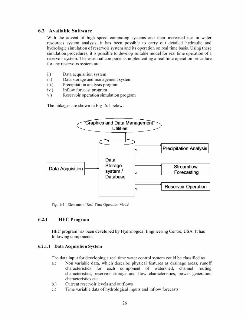
26

6.2 Available Software With the advent of high speed computing systems and their increased use in water resources system analysis, it has been possible to carry out detailed hydraulic and hydrologic simulation of reservoir system and its operation on real time basis. Using these simulation procedures, it is possible to develop suitable model for real time operation of a reservoir system. The essential components implementing a real time operation procedure for any reservoirs system are:

i.) Data acquisition system ii.) Data storage and management system iii.) Precipitation analysis program iv.) Inflow forecast program v.) Reservoir operation simulation program

The linkages are shown in Fig- 6.1 below:

Graphics and Data ManagementUtilities

Data Acquisition

Precipitation Analysis

StreamflowForecasting

Reservoir Operation

Data Storage system / Database

Graphics and Data ManagementUtilities

Data Acquisition

Precipitation Analysis

StreamflowForecasting

Reservoir Operation

Data Storage system / Database

Fig.- 6.1 : Elements of Real Time Operation Model

6.2.1 HEC Program HEC program has been developed by Hydrological Engineering Centre, USA. It has following components.

6.2.1.1 Data Acquisition System

The data input for developing a real time water control system could be classified as a.) Non variable data, which describe physical features as drainage areas, runoff

characteristics for each component of watershed, channel routing characteristics, reservoir storage and flow characteristics, power generation characteristics etc.

b.) Current reservoir levels and outflows c.) Time variable data of hydrological inputs and inflow forecasts

27

d.) Water demands for various purposes and project regulation criteria for each period from the knowledge of existing conditions.

Among the above data inputs, time variable data are of prime importance in real time operation. Thus the data collection system for real time operation of the reservoirs has to be designed primarily for observation and transmission of these data. The time variable data may be classified into

a.) Hydro-meteorological data b.) Project data The hydro-meteorological elements that may be observed are water levels in rivers and reservoirs, run-off at various G&D sites and precipitation. The time variable project data include spillway and outlet gate opening positions, hourly power generation and other water control parameters that are required for project regulation. The time variable data can be observed and transmitted through manual, semi-automatic, or automatic systems. Historically, manual observation represented the backbone of the hydrometeorological data collection and transmission system. Manual handling of data may be adequate for smaller basins, but the chances of errors in repetitive transmission of data from source to the end-user, time required for transmission, inability to physically process the vast amount of data from different sources usually dictate the installation of automatic systems. However, even with the installation of automatic systems, there may be a need for manual or semi-automatic data interrogation equipment to backup the automated systems.

6.2.1.1.1 Manual Data System In this system, manually observed data are transmitted by voice to water control managers through telephone / wireless / microwave system. In large river basins, the network may consist of several sub-systems, through which data may have to be repeatedly transmitted to control center. Repeated transmission of data from source to the end-user may increase the chances of errors.

6.2.1.1.2 Semi-Automatic Systems Semi-automatic transmission systems are those which have automated part of data collection system, but still need presence of an individual for complete functioning. The transmission of data could be through any medium available as in the case of manual system.

6.2.1.1.3 Automatic Data Systems The first automated observation and storage capabilities at field sites used analog methods. At a gauge station this typically included a float system to drive a pen recorder. Such a system produced an automatic analog record of water levels. With the availability of digital technology, the same float is used to drive a digital shaft encoder whose output is stored in memory of a local microprocessor at the gauging site, known as Data Collection Platforms (DCP). The precipitation is usually observed through sensors, which record the pressure exerted by the water / snow pack into DCPs which automatically transmit the data stored in the memory at user defined intervals to the central processing unit.

28

6.2.1.2 Data Storage and Management System

Several conventional general purpose data storage systems are commercially available. The Data Storage System (DSS) provides a means for storing and maintaining data in a centralized location, providing input to and storing output from application programs, transferring data between application programs and displaying the data in graphs or tables. The DSS has capabilities to store data in a fashion convenient for inventory, retrieval, archiving and model application. The DSS uses a block of sequential data as the basic unit of storage. This concept results in a more efficient access of time series or other uniquely related data. Each block contains a series of values of a single variable over a time span appropriate for most applications. The basic concept underlying the DSS is the organisation of data into records of continuous applications related elements, as opposed to individually addressable data items. This approach is ore efficient for water resources applications, than that of a conventional database system, because it avoids the processing and storage overhead required to assemble an equivalent record from a conventional system. The management of data essentially consists of entry of the data received into the data base, checking consistency, mathematical / statistical manipulation, editing and house keeping of the data.

6.2.1.3 Precipitation Analysis Program

One of the inputs to the stream flow forecast program is the basin average hyetograph, assessed from the real time rainfall data. Usually the basin average rainfall hyetograph is calculated using Thiessen polygon method. In real time operation mode, often rainfall data from all the stations in the basin may not be available at any instant of time, due to practical problems as failure of the reporting station, delay in data transmission etc. As the weights for calculation of average hyetograph depend on the number of rainfall stations considered, the Thiessen weights may vary from time to time according to the number of stations reported. Calculation of the weights each time according to the rain gauges reported at the time of preparing for forecast is cumbersome and time consuming. The delay in computation of average rainfall hyetograph may cause delay in flood forecast and consequently delay in taking release decision. The precipitation analysis program PRECIP, on the other hand automatically calculates the basin average hyetographs from the rainfall data reported at any instant, using a convenient method other than Thiessen polygon.

6.2.1.4 Inflow Forecast Program

The surface run-off response of a river basin to precipitation could be effectively assessed by representing the basin as an interconnected system of hydrological and hydraulic components and simulation of the model. The model of river basin, known as ‘ stream network model ’ could be developed using HEC1 flood hydrograph computer software package. The HEC1 models an aspect of the precipitation-runoff process of each component within a portion of the basin, commonly referred to as a sub-basin. The

29

result of the modelling process is the computation of stream flow hydrographs at desired locations. The model developed, calibrated and verified could be used for real time flood forecast at desired locations.

The HEC1 computer program was developed by Hydrological Engineering Centre, USA. The entire HEC1 package and its forecasting version HEC1F have been implemented in Bhakra Beas system study.

The HEC1 stream network model developed for the basin is the foundation for runoff forecast. With this model, real time forecast is achieved through the application of HEC1F program, which is the forecast version of HEC1 program. The HEC1F program is run in two separate applications. In the first application, the program re-estimates parameters for gauged headwater catchments using the real time data and calculates runoff hydrographs with these updated parameters. In the second application, HEC1F calculates discharge hydrographs for ungauged catchments with the user defined parameters and are routed and combined through out the basin. The hydrographs are also blended with the observed hydrographs at each gauge, prior to subsequent routing and combining operations. For all these applications the sub-basin average precipitation hyetograph computed by PRECIP is the primary input.

6.2.1.4.1 Rainfall-Runoff Simulation The HEC1 model components could be used to simulate the rainfall runoff process as it occurs in an actual river basin. The model components are based on simple mathematical relationships, which are intended to represent individual meteorologic, hydrologic, and hydraulic processes involving the precipitation runoff process. These processes can be grouped into precipitation, interception / infiltration, transformation of precipitation excess to sub-basin outflow, addition of baseflow, and flood hydrograph routing.

6.2.1.4.2 Flood Routing Flood routing is used to simulate flood wave movement through river reaches and reservoirs. Most of the flood routing methods available in HEC1 are based on the continuity equation and some relationship between flow and storage or stage. These methods are Muskingum, Muskingum-Cunge, Kinematic Wave, Modified Pulse, Working R&D, Level Pool reservoir routing. In all these methods, routing proceeds on an independent-reach basis from upstream to downstream and neither backwater effect nor discontinuities in the water surface such as jumps or bores are considered.

The Muskingum-Cunge and Kinematic Wave techniques could be used to route an upstream hydrograph independent of lateral inflow. None of the methods is available when the channel hydraulics are affected by backwater conditions. This limitation exists for all routing methods incorporated into HEC1 because of the headwater nature of the model.

In general, the Muskingum-Cunge method (an approximate diffusion router) is a superior and more preferable technique than the Kinematic wave method for channel routing, particularly when there is no lateral inflow to the channel. However, if applied, the Kinematic Wave channel routing method should be used for relatively short routing reaches (e.g. those encountered in urban watershed studies) in headwater areas. Routed hydrographs produced under these circumstances should show at the most five percent

30

peak discharge attenuation due to numerical errors in solving the kinematic wave equations. Peak attenuation greater than this amount probably indicates the formation of a kinematic wave ‘shock’ which is not desirable. Under these circumstances, the user should either reformulate the watershed model so that lateral inflow exists in the routing reach, or more preferably, utilise the Muskingum-Cunge method.

6.2.1.4.3 Pumping Plants Pumping plants may be simulated for interior flooding problems, where runoff ponds in low areas or behind levees, flood walls etc. Multiple pumps may be used, each with different on and off elevations. Pumps are simulated using the level-pool reservoir routing option. The program checks the reservoir stage at the beginning of each time period. If the stage exceeds the ‘pump on’ elevation, the pump is turned on and the pump outlet is included as an additional outflow term in the routing equation. When the reservoir stage drops below the ‘pump off’ elevation, the pump is turned off. Several pumps with different on and off elevations could be used.

Each pump discharges at a constant rate and could be either on or off. Variation of discharge with head is not considered in HEC1. The average discharge for a time period is set to the pump capacity, so it is assumed that the pump is turned on immediately after the end of the previous time period.

Pumped flow may be retrieved at any point after the pump location in the same manner as a diverted hydrograph.

6.2.1.4.4 Real Time Forecast The HEC1 Stream Network model developed for the basin is the foundation for runoff forecast. With this model, real time forecast is achieved through the application of HEC1F program, which is the forecast version of HEC1 program. The HEC1F program is run in two separate applications. In the first application, the program re-estimates parameters for gauged headwater catchments using the real time data and calculates runoff hydrographs with these updated parameters. The input for this step of application is referred as the HEC1E model. In the second application, HEC1F calculates discharge hydrographs for ungauged catchments with the user defined parameters and are routed and combined through out the basin. The hydrographs are also blended with the observed hydrograph at each gauge, prior to subsequent routing and combining operations. For all these applications the sub basin average precipitation hyetograph computed by PRECIP is the primary input.

6.2.2 Acres Reservoir Simulation Program (ARSP) ARSP is a general ‘multi-purpose, multi-reservoir simulation’ program. The ARSP formulation is capable of simulating a wide range of operating policies governing the allocation of water in a multi-purpose, multi-reservoir system. The program is based on the premise that a water resource system can be represented by a flow network and that an optimal operating decision for the upcoming time period can be made given the initial state of the system and estimates of net inflows during the period.

Since the network solving algorithm in ARSP is a subset of linear programming, it is subject to the same limitations. For instance, all constraints must be linear and consequently all non-linear relationships, such as volume-elevation curves, tail water

31

rating curves, efficiency curves, head loss functions etc. which may occur in a water resources system must be described by several piecewise linear segments.

In ARSP a physical water resource system is represented as network schematic consisting of discrete components each of which is separately represented in the model. Junctions and control points, such as reservoirs are represented as nodes, while natural or manmade flow paths that connect junctions are referred to as channels. Each channel which connects two nodes is represented in the computer model as either a flow channel or a demand channel. A flow channel can have its full flow carrying capacity broken up in to a number of discrete ranges. Each range can have user specified bounds and a penalty to reflect the relative desirability of having flow in that range. Demand channels, on the other hand, have user prescribed penalties associated with not meeting the imposed demand. The amount of water shortage in each demand channel is multiplied by the respective penalties assigned. In the case of reservoirs, discrete intervals of reservoir storage, known as zones are defined. Each storage zone has a specified upper and lower boundary and a user specified cost referred to as a penalty that represents the relative value of water stored in the zone. So that if the water level is in a particular zone then it will attract a penalty of that zone multiplied by the amount of water in that zone. The conservation zones have a lower penalty or sometimes a negative penalty (benefit) so that the water remains in the conservation zones. The Spill, Flood, and Dead storage zones have high penalties so that the water level does not enter in these zones.

The network solution technique routes water in such a way that the total demand and reservoir storage penalties are minimised for a given time step. ( e.g. the model decides if it is preferable to draw a reservoir down to maintain a minimum flow in a channel or to allow a channel flow to fall below the desired value).

Representing reservoir zones, demands and channel flow ranges in this manner permits the study of trade-offs in a water resource system subject to different operating policies. The policies reflect the operation strategy employed to optimize benefits within a water resource system and are represented in the model by penalties assigned to flow occurring in channels or water remaining in reservoir storage. Any water resource system must be described in two ways, namely: i.) Representation of the water resource system by a network; ii.) Representation of the water resource operating policy by a penalty structure. This approach allows for alternative water resource policies to be investigated by superimposing new penalty structure on the existing network. In the current general form, the model uses a monthly computational time step.

6.2.2.1 Hydrologic Data Requirement

ARSP requires a hydrologic data series which consists of: • monthly inflow (basin runoff) time series at specified reservoir nodes, with or

without storage;

32

• monthly precipitation time series at specified reservoir nodes; and • mean monthly evaporation at specified reservoir nodes.

6.2.2.2 Other Data Requirement

Other data requirements include • number of reservoirs and nodes (with inflow); • number of net basin inflow series; • number of precipitation gauge stations; • codes to specify units of basin runoff; • full reservoir area Mm2; • reservoir reference numbers for rainfall and inflow series; • Monthly Domestic and Industrial water demand at various nodes; • Monthly Irrigation water demand at various command areas; • Monthly Hydropower generation demands at various powerhouses; • Monthly minimum flow requirement in various river reaches; • Power house and turbine features; • Irrigation return flows; etc ARSP has no built-in capability for generating stochastic stream flows; consequently, inflow series must be externally derived. This data can be entered in any one of the following four units. • as total inflow in m3/s or Mm3 • as inflow per unit area in m3/s/Mm2 or Mm3/Mm2. Monthly precipitation data for the full simulation period are required for reservoirs with storage. These data are combined with a rainfall-runoff coefficient to determine the runoff contribution from rainfall on the reservoir surface area, as well as the surface area exposed when levels are low. Mean monthly evaporation coefficients (mm/month) are entered for each reservoir. The coefficients reflect the average depth of water lost to evaporation from the surface area of each reservoir on a monthly basis. In any time period, the net inflow to a reservoir is calculated as the net basin runoff and the net contribution from rainfall, both on the reservoir surface itself and at low levels on the exposed reservoir bed, less the evaporation. The water balance over the area occupied by the storage reservoir at full supply level (FSL) is considered separately from the net inflows. When evaporative losses are large, care is required to ensure that the overall water balance is treated correctly, and that ‘double counting’ does not occur.

6.2.3 RIBASIM Program RIBASIM is a generic model package for simulation of the behaviour of river basins during varying hydrologic conditions. The model is a comprehensive and flexible tool

33

to link the hydrologic inputs of water at various locations to the various water-using activities in the basin and to evaluate a variety of measures related to infrastructure and operational management. It provides an efficient handling and structured analysis of the large amounts of data commonly associated with water resources systems. RIBASIM has been developed and fine-tuned at WL | DELFT HYDRAULICS in the course of many projects. The variety of applications have resulted in a versatile model; modelling elements (e.g. reservoir operation, irrigation water use, low flow requirement, etc.) can be selected from a library of options which can easily be expanded to include further options. Delft tools offer a number of MS Windows based graphical analysis tools which can be used in a flexible way depending on the model application. The complete system enables a quantitative analysis of the various aspects, includes systems to structure the required data, and presents model calculations. The know-how, structuring, and methodology included in RIBASIM can be schematised as shown in Fig. 6.2.

Fig.- 6.2 : Structure of RIBASIM program

The sub-systems are:

• An object oriented data base system containing data describing the WRS including the data base management system;

• A set of application models describing the different components in the planning process;

• An analysis system containing various tools for structuring the analysis process and the visualisation & interpretation of the results;

• A graphical user-interface.

34

Purpose of the different models and programs are: HYMOS: a data base management system for storage, retrieval, processing, and analysis of hydrological data. HYMOS is a separate WL | DELFT HYDRAULICS software package, being implemented in India under World Bank aided National Hydrology Project. SAMO: determines the runoff of non-irrigated areas per water district and per time step, based on time series of potential evapotranspiration and rainfall. SAMO is part of the HYMOS software. AGWAT: determines the irrigation water requirements and return flows per irrigation node and per time step under full supply condition for a variety of cropping patterns, taking into account farming and irrigation practices, and physical parameters related to soils and hydro-meteorological characteristics. More in detail the following factors are taken into account: • reference evapotranspiration, and expected and actual rainfall data; • percolation losses and readily available soil moisture; • crop factors for various stages of crop growth, and cropping calendars; • water requirements for land preparation; • spatial distribution of cropping patterns; • maximum allowed and target field water levels for each crop; • staggering periods and starting dates for land preparation; • spatial distribution of golongan systems; • irrigation efficiency and re-use of drainage water; and • spatial distribution of irrigation systems. FISHWAT: determines fresh and saline water requirements of brackish water fish ponds under full supply conditions, taking into account various species per water district and per time step to be cultivated, production technology, climatological characteristics, and salinities of the supplied water. Water demands are derived from water and salt balances. DEMES: estimates the demand for domestic, municipal & industrial water supply based on projections of population and water using activities, a mode split between surface and groundwater, losses during transport and treatment, the applied level of technology, maintenance and management. DEMES is not included in the DSS RIBASIM being used in this study. RIBASIM: computes the water distribution in the main distribution network and inside the water district by simulating the river and canal flows, operation of reservoirs (including hydropower production) and diversion structures. The model simulates the water allocation to the water users within the water districts and within a river basin. For the water districts, the allocation is based on: • water demands for irrigated agriculture (AGWAT), brackish water aquaculture

(Fishwat), domestic, municipal and industrial water supply (DEMES); • runoff from the non-irrigated part of the water district (SAMO); and • water management rules for the allocation of water over various users. For the river basin, the allocation is based on : • water demand of all water users extracting water from the main distribution

system (network);

35

• water availability (supply); • characteristics of water distribution and storage facilities (infrastructure); • operation rules for water distribution and storage facilities like reservoirs,

canals, pumps, weirs and siphons; and • water management rules followed in the allocation of water over various users

in case of water shortages (allocation priorities). WADIS: determines the potential and actual crop yield, production costs of irrigated and rainfed agriculture per crop, and brackish water aquaculture in each water district. DELWAQ: determines the composition of the flow in any location of the main distribution network (rivers and canal system) which forms a first insight in the quality of the water at that location. The model can be used as well to predict the water quality in the main distribution network under various hydrological conditions, pollution and sanitation scenarios. Only fraction simulation aspect of DELWAQ is included in the version of RIBASIM available under HP. WLM (Waste Load Model): estimation of the actual and future waste loads (point and non-point sources) on surface water. WLM provides direct input to the DELWAQ simulation model. Not included in the version of RIBASIM available under HP. STRATIF: simulation of stratification layers in reservoirs. Not included in the version of RIBASIM available under HP.

6.2.3.1 When to use RIBASIM The types of analysis addressed by the model are the following: • evaluation of the limits on resources and/ or the potential for development in a

region or basin, given the available water resources and their natural variations, to what extent can a river basin be developed in terms of reservoirs, irrigation schemes, water supply systems, while avoiding unacceptable shortages for users? When and where will conflicts between water users occur? Which combination of infrastructure and operational management will provide an optimum use of the available resources?

• evaluation of measures to improve the water supply situation such as measures concerning changes in the infrastructure, operational management, and demand management; and

• evaluation of the origin of water for every location in the river basin as a first step towards an actual water quality analysis, without the necessity of having available information with regard to waste loads, waste water discharges and water quality of (upstream) sources, the effect of measures on the distribution of water from the various sources in the basin is calculated (influence area of a source of water).

Simulation of the water balance of the region/basin forms the basis for such analysis. RIBASIM provides the means to prepare such balance with sufficient detail, e.g. taking into account re-use of water, and with facilities to vary the simulated configuration and to process results.

36

6.2.3.2 Model Schematisation

To perform river basin simulations with RIBASIM, a model schematization of the study area is prepared in the form of a network, consisting of nodes connected by links. Such a network represents all the features of the basin that play a role in its water balance. Four main groups of schematization elements are differentiated in the model: • Infrastructure, both natural and man-made (reservoirs, lakes, rivers, canals,

surface water and groundwater pumping stations, pipelines); • Water users, or in a wider sense: water related activities (domestic, municipal

and industrial water supply, agriculture, hydropower, aquaculture, navigation, recreation, nature);

• Management of the water resources system (operation rules for reservoirs and diversions, priorities and proportional water allocation, minimum flows in certain river stretches for sanitary or ecological reasons); and

• Hydrology i.e. inflows to the system, inter-basin flows, precipitation and evaporation

The nodes of the network represent structures, water users, inflows and so on; the links represent transport of water between the different activities or water bodies (interaction between river reaches or surface water reservoirs and aquifers or among aquifers).

6.2.3.3 Simulation Simulations are usually made to analyse a specific (future) condition over long series of historical years to cover sequences of dry and wet periods. The simulation proceeds in time steps, of typically one month, half a month or 10 days. In essence, RIBASIM is a water balance model. Within each time step a water balance calculation is made, in two phases: • Target setting phase (demand phase)

Determination of all the water demands, resulting in targets for the releases from surface water reservoirs, aquifers, and diversion flows at weirs & pumping stations.

• Water allocation phase (supply phase). Allocation of water over the users according to targets, availability, and allocation rules.

Water allocation to users can be implemented in a variety of ways: in its simplest form, water is allocated on a "first come, first serve" principle along the natural flow direction. This allocation can be amended by rules which e.g. allocate priority to particular users or which result in an allocation proportional to demand. On the basis of a set of simulations, usually made for a range of alternative development or management strategies, the performance of the basin is evaluated in terms of water allocation, shortages, (firm) energy production, overall river basin water balance, water district crop yields and crop production costs, etc.

37

6.2.3.4 Model Structure The preparation of input data, running of the model and the processing of output data into graphs, maps of the study area, diagrams and tables take entire place via user-friendly menu screens. RIBASIM distinguishes a number of standard nodes and link types with which the river basin network can be constructed. Each type of node and link correspond to a particular part of the model that handles the relevant computations for this type of node or link. The model contains a library of nodes and links that can easily be expanded to include other activities specific to a particular basin. A short selection of available "node" and “link” features is presented below: • irrigation areas: computation of water demand on the network taking into

account crop characteristics, irrigation practice parameters, and actual rainfall; • conjunctive use of groundwater and surface water for various water users like

irrigation and public water supply; • water balance of aquifers; • pumping capacity and maximum groundwater depth for abstraction from an

aquifer; • brackish or fresh water aquaculture: flushing demands; • minimum flow requirements for sanitation, navigation or ecology; • loss flow from river stretches to groundwater; • run-of-river power plants; • hydropower production requirements at surface water reservoirs: firm

(guaranteed) and secondary energy, scheduling; • computation of pumping energy (from groundwater or surface water to users); • return flows from users (agriculture, aquaculture, public and industrial water

supplies); • additional (backwater) abstractions from surface water reservoir for various

water uses; • surface water reservoir operation rules (firm storage, target storage e.g. for

average maximum energy generation, flood control storage); • sub-catchments (water districts) which form a hydrological unit from the

viewpoint of water supply and demand; • hydraulic description of (part of) river stretches and partitions of surface water

reservoir.

6.2.3.5 Input Requirement of RIBASIM Input for RIBASIM covers the following subjects: • river basin network schematization: location of surface water reservoirs,

aquifers (groundwater reservoirs), irrigation areas, diversion weirs, (river) channels, DMI channels, sub-catchments comprising a system of nodes and links;

• model data characterising each node and link in the schematization;

• preferred sources of water for the identified water users in the basin;

38

• water allocation rules and operation rules for surface water reservoirs and diversions;

• hydrologic data (time series of available flow at the system boundaries e.g. from inter-basin transfers, open water evaporation, rainfall, general district water demand and discharges, water district runoff).

6.2.3.6 Output of RIBASIM

Simulation results can be processed with a number of standard post-processors into graphs, spreadsheets, maps, and tables. For a quick visual interpretation of results, a number of graphs can be produced on screen (e.g. during calibration testing). The form of the graphs can be adapted according to the user requirements. Graphs show e.g. the applied cropping pattern, the water allocation, the shortages per user, the actual surface or groundwater reservoir storage, the overall water balance of the basin, and the energy production. The results can be further processed with spreadsheet software like MS Excel or directly included in reports produced e.g. with MS Word. Tables range from summaries of the main results (success rate, allocated amounts of water, water shortages, water utilisation rate, failure year percentage, and energy production) to user-defined tables with detailed results per time step for specific variables per node or link.

6.2.3.7 Interaction with other Programs RIBASIM can be used in combination with other WL | DELFT HYDRAULICS software, such as: WLM (WASTE LOAD MODEL) : Estimation of actual and future waste loads (point and non-point sources) on surface water. It provides direct input to the DELWAQ simulation model.

DELWAQ (DELFT WATER QUALITY MODEL): Water quality simulation model; calculates the behaviour and fate of water quality constituents based on scenarios which have been formulated as input and which have been translated into a flow pattern and waste loads. DELWAQ can use the same schematization as RIBASIM and is tuned to use the flow pattern produced by RIBASIM. HYMOS (HYDROLOGICAL MODELLING SYSTEM): Data base management and data processing software package for hydro-meteorological data. It enables to set up a convenient structuring of data and provides an extensive set of tools for data entry, validation, completion, analysis, retrieval, and reporting.

39

STRATIF (STRATIFICATION MODEL): Model for the simulation of stratification layers in reservoirs (still under development).

6.2.3.8 Computational Framework Depending on the complexity of the water resources system to be analysed, a variable

set of coherent models can be used for the quantitative analysis of the water resources system, measures, and strategies. This set of models and related databases forms the “computational framework” or Decision Support System. The Decision Support System used in the study is DSS RIBASIM developed by WL | DELFT HYDRAULICS (Fig. 6.3).

DSS RIBASIM is a generic model package for simulation of the behaviour of river

basins during varying hydrologic conditions. The model is a comprehensive and flexible tool to link the hydrologic inputs of water at various locations to the various water-using activities in the basin and to evaluate a variety of measures related to infrastructure & operational management. It provides an efficient handling and structured analysis of the large amounts of data commonly associated with water resources systems.

Fig.- 6.3 : Computational Framework of RIBASIM

40

The core of DSS RIBASIM is a River Basin simulation model RIBASIM. The main RIBASIM user interface is presented as a flow diagram of blocks (Fig.6.4) representing the tasks to be carried out and their order to complete the simulation process. The interface guides the user through the analysis from data entry to simulation. The task blocks change colour on the computer screen to show the user which tasks have been completed, which are in progress, and which are yet to be carried out. The conceptual and computational framework thus developed is used to analyse relationships between water quantity and water quality issues, between land use and water resources development, and between ecosystem development and socio economic activities in the study region taking into account social, environmental, and economic objectives. The framework also provides support for policy formulation regarding WRM objectives and the development of strategies needed to reach these objectives. The purpose of the analysis is to prepare and support decisions. The analysis is iterative and cyclic.

Fig.- 6.4 : Main RIBASIM user interface

41

7 CASE STUDIES

7.1 Bhakra-Beas System

This study of “Real Time Integrated Operation of Bhakra Beas system” was conducted in BPMO, CWC in 1996 using the HEC group of programs. The Bhakra Beas system in the Indus basin has a number of multi purpose reservoirs and diversion structure with unique characteristics as runoff due to rainfall and snowmelt, interstate water sharing aspects, inter basin transfer of water etc. Thus this system was considered as an ideal system for development of Real time operation technique and demonstrating its capability. The same has been successfully developed for the system. The Bhakra Beas reservoirs system regulates the waters of Sutlej, Beas and Ravi of the Indus basin. The Sutlej river after traversing through Tibet crosses into India and flows towards Bhakra gorge. The Bhakra dam exists in this portion of the river. The Beas river joins Sutlej at Harike. The Pandoh and Pong are the two important projects in the Beas basin. The Pandoh dam diverts Beas water to Sutlej for generation of power and supplementing the Bhakra reservoir. The Pong dam, though primarily designed for meeting the irrigation demands of Rajasthan, Punjab and Haryana , is also used for power generation and flood control. The Bhakra Beas projects in the Sutlej Beas system comprises two major projects namely the Bhakra Nangal project on the Sutlej and the Beas project on the river Beas. The Bhakra Nangal project comprises the Bhakra dam, the Nangal dam (13Kms. d/s of Bhakra dam ), the Nangal Hydel channel, Ganguwal and Kotla power houses, Anandpur Sahib power channel and its two power houses. While the Beas project comprises two projects namely the Unit I : Beas – Sutlej link and the Unit II : Beas dam at Pong. The index map of Bhakra Beas system is shown in Fig-7.1

Fig.- 7.1 : Index map of Bhakra-Beas reservoir system

42

7.1.1 Bhakra Dam

The Bhakra dam, is constructed across river Sutlej at the Bhakra gorge. The reservoir created by the dam, known as Gobind Sagar, has a gross storage capacity of 9621 Mm3 and a water spread area of 168.35 Mm2. The catchment area upto the dam is 56,980 Mm2. It is a multipurpose dam serving the needs of irrigation, power, flood control and pisciculture. There are two Power Houses at Bhakra, one on the left side and the other on the right side. The total installed capacity of these plants is 1200 MW. The Power Houses are being operated in conjunction with the Ganguwal and Kotla Power Houses on the Nangal Hydel channel.

7.1.2 Nangal Dam

The Nangal Dam, situated at about 13 km downstream of the Bhakra dam, diverts water released from Bhakra into the Nangal Hydel Channel and also feeds the Anandpur Sahib Hydel Channel of Punjab State for power generation and irrigation needs. The pond created by the dam acts as a balancing reservoir to smoothen out the diurnal variation in releases. Just upstream of the Nangal dam, two hydel channels by name Nangal Hydel Channel and Anandpur Sahib Hydel Channel take off from the left bank of the Sutlej. The Nangal channel diverts water for power generation at Ganguwal and Kotla power houses, by utilizing the natural falls available along the channel. The Ganguwal power house is located about 16 km from Nangal and the Kotla power house at 10 km downstream of Ganguwal. These two power houses together generate 154 MW of power. The water released after power generation is utilised for irrigation in Punjab, Haryana and Rajasthan, though the Bhakra Main Canal. The Anandpur Sahib Hydel Channel has two power houses of 67 MW each.

7.1.3 Beas-Sutlej Link

The Beas Sutlej Link envisages diversion of 4716 Mm3of Beas water into the Sutlej for power generation, by utilizing a difference in head of 320 m. The water diverted also makes up any shortage of water in the Bhakra reservoir and provides canal irrigation in Gurgaon and other southern districts of the Haryana State. The project comprises the diversion dam at Pandoh, the Pandoh Baggi Diversion Tunnel, the Baggi Control Works, the Sunder Nagar Hydel Channel, the Sundernagar Balancing Reservoir, the Sundernagar Sutlej Tunnel and the Power House at Dehar.

7.1.4 Beas Dam at Pong

The Beas Dam is located at Pong, which was a tiny hamlet on the high bank of Beas in Kangra district of Himachal Pradesh. The reservoir created by the dam has a gross storage capacity of 8570 Mm3 and a live storage of 7290 Mm3. Though the project has been designed primarily for meeting the irrigation demands of Rajasthan, Punjab and

43

Haryana, it is being used for power generation and flood control also. The Pong Power Plant has a capacity of 360 MW.

7.1.5 Irrigation System

Downstream of the Nangal, two headworks are existing on river Sutlej, one at Ropar and another at Harike. The headworks at Ropar picks up the water released in the Sutlej at Nangal and through the escapes from the power houses on Nangal and Anandpur Sahib Power Channels. The water reaching Ropar is diverted for irrigation in Punjab, through the Sirhind canal system. The headworks at Harike, located just downstream of the confluence of Beas with Sutlej, picks up water released downstream of Ropar and from Pong dam on Beas. It also receives water diverted from Ravi at Madhopur though the Ravi Beas link. The water reaching the headworks is utilised for irrigation in Punjab and Rajasthan through the Rajasthan, Sirhind and Ferozpur feeder canal systems. The Harike headworks has been considered as the terminal control structure for the purpose of the study.

7.1.6 Existing Operation

Reservoir operations in the Bhakra Beas system constitute controlled release of water downstream of the Bhakra dam in relation to the inflow into the Gobindsagar, the available storage and the condition of flooding of downstream channels, so as to fulfil the design requirements of the system with respect to irrigation, power and flood control etc. The period from 1st June to 20th September is the filling period and from 21st September to 31st May is the depletion period, when water is released from reservoir to meet the conservational and other demands. During the filling period, irrigation demands are met in full, subject to the constraint that the reservoir is not allowed to deplete at any time. This means that the demands could not be met fully if they exceed the inflows. This could happen because of the delayed arrival of the monsoon, failure of monsoon and also in case of dry years. Because the demands could not be met in full in all the years, based on the Power Studies carried out by the BBMB a decision is taken on the 21st September regarding regulation of supplies from the reservoir during the depletion period. The maximum intensity of the routed floods passed downstream of the dam would be of the order of 8,212 m3/s, being the maximum design discharge intensity of the spillway. The maximum storage level of Gobindsagar is at EL.515.11m above MSL and is permitted to be achieved only when the early flood warning system is established and working properly. During the period when the early flood warning system is not in operation (as is the present situation), the maximum permissible reservoir elevation is to be maintained at EL 512.06 m above MSL. With this maximum permissible reservoir elevation, prior depletion of the reservoir in anticipation of the incoming flood would not be required and the flood would be routed by allowing temporary rise in level upto 515.11m.

44

When the early flood warning system is operative and the reservoir is permitted to be build up to the maximum EL. 515.11m above MSL, the reservoir is to be depleted to the required extent in anticipation of the incoming flood and the flood routing should be carried out in such a way that the reservoir level never rises above EL. 515.11 m.

7.1.7 Real Time Forecast Model For the real time operation of the reservoir system, the forecast of inflows from the catchment upstream of the Bhakra Dam is of prime importance. In addition, the inflow forecast for the catchments of two downstream Khads viz., Swan and Sirsa are very decisive, as the releases from the Bhakra dam are to be controlled according to the flood conditions of these two khads, to prevent down stream areas from flooding. Thus the conditions of these two khads, to prevent down stream areas from flooding. Thus the inflow forecast model was developed for the Bhakra dam catchment and for these two khads using the HEC 1 program. The actual forecast of unregulated stream run-off could be achieved using the computer program HECIF, which is the forecast version of the computer program HEC1 For the purpose of development of stream network model for the Bhakra dam catchment, it was divided into eight sub-basins. This delineation was done based on the consideration of (i) the location of the control points (ii) the location of the precipitation and flow gauging stations and (iii) the geographic, hydrographic and meteorological variability within the basin.

The Snyder unit hydrograph parameters, loss rates and routing parameters for all the sub-basins/channels were optimized, using the capabilities of HEC-1 package. Subsequently the model was calibrated with these runoff and routing parameters optimized using data of the historical events. For working out the weighted average precipitation of various sub-basin the PRECIP program was also implemented. The forecast model was tested with various historic flood events and forecast worked out using HEC1F model. The results compared well with the observed data.

7.1.8 Real Time Reservoir Operation

For real time operation of Bhakra Beas system simulation models for flood control and conservation were developed using HEC5. These models were used in conjunction with HEC1F forecast program. The flood control simulation model was developed by including Bhakra reservoir, Nangal pond, Ropar and Harike headworks, Swan Nadi and Sirsa Nadi confluences with Sutlej, Nangal and Anandpur Sahib Hydel channels and their return flows to Sutlej river. A wide variety of reservoir operation options that affect release decisions were studied through simulation of this model. These included maximum channel capacities at downstream control points, emergency conditions requiring pre-release, minimum flow requirements, variable foresight etc. The model was accordingly calibrated, tested and made operational with various input options.

45

7.1.9 Testing of Models

Using the historical precipitation data stored in the Data Storage System (HECDSS), various applications of HECIF was made and inflow hydrographs were stored in HECDSS. In the next sequential application, using the forecasted hydrographs stored in HECDSS, reservoir operation was simulated by HEC5 models according to the pre-defined operating policy and user defined constraints. Such sequential application of HEC1F and HEC5 models in conjunction with HECDSS gave very comparable simulation results. It could also be perceived that through sequential application of the models as and when required reservoir operation simulation could be done and results analysed well in advance for taking appropriate operational decisions. The real time reservoir operation techniques now developed, thus help in efficient and optimal integrated operation of reservoir system for deriving maximum benefits of flood control and conservation.

7.1.10 Lessons learnt during Bhakra Beas system case study

In view of the above, the following lessons are learnt during this case study:

• As far as possible the reservoirs be planned and operated in an integrated manner for the basin as a whole;

• At present real time operation models were developed using the water control

software of HEC. A number of models developed by other agencies are also available for implementing the procedure. It would be desirable to implement real time operation procedure using other appropriate models, after modifications to suit Indian conditions;

• The efficiency of the real time operation of a reservoir system mainly depends upon the data observation and transmission network in the basin. As far as possible efforts be made to install automatic data collection and transmission system;

• Balance should be maintained between temptations to model in extreme detail or to model with assumptions so gross as to eliminate the usefulness of the analysis. The methodology needs to be adapted to suit particular situations to achieve the desired objectives and to assist the decision maker; and

• Close co-ordination between various data collection and management agencies, water control managers, reservoir operation field staff and water use agencies be maintained for effective and efficient water utilisation.

7.2 Ukai-Kakrapar System This study on Integrated Operation of Ukai-Kakrapar sub-system in Tapi river basin was conducted in BPMO in June-2000 using ARSP program which works on monthly timestep.

46

7.2.1 System, Network, and Objective The Ukai multipurpose project on river Tapi in Gujarat was completed in 1973 to provide benefits of irrigation, hydropower generation and partial flood control. The dam was designed to cope with SPF of 43,490 m3/s and PMF of 59.920 m3/s. The spillway has the capacity to pass 37,859 m3/s at FRL and 46,269 m3/s at MWL. On the other hand Safe Carrying Capacity of the river on the d/s was considered to be of the order of 24,069 m3/s. Construction of flood embankments along the Tapi River d/s was contemplated to protect the low lying areas of the countryside and Surat city. These embankments are completed only partially till now.

The flood which occurred during September, 1998 resulted in heavy losses in the Surat city, though the flood peak was only about 29,817 m3/s. The Safe Carrying Capacity of the Tapi river near Surat is reported to have been significantly reduced due to encroachment in the flood plain areas, silting in the river bed and effluents caused by Singanpur weir constructed on the river close to the city. It is assessed that the river at Surat can not carry only 11,327 m3/s without causing significant damages. Thereafter, a Committee was formed to prepare the flood control operation manual for Ukai reservoir under the Chairmanship of CE (HSO) and members from CWC and Government of Gujarat. The Committee in April, 2000 suggested a rule curve for operation of Ukai reservoir in view of the flood irrigation for Surat City.

The schematic of the system is as given if figure 7.2:

Fig.- 7.2 : System Schematic for Ukai-Kakrapar System in Tapi Basin

In the study, attempt was made to maximize flood cushion without hampering fulfillment of water supply, Irrigation or Power Demands to be met from Ukai-Kakrapar System. Main objective of the study were:

• To meet irrigation demands at 75% dependability

2

3

4

5

6

Ukai Reservoir and Powerhouse

Ukai Command area

Kakrapar Command area

Surat city water supply

Sea

Kakrapar weir

Singanpur weir

1

Inflow

Inflow

Inflow

47

• To meet water supply demand of Surat City at 95% dependability • To meet firm power demand (65 MW) at Ukai Power House at 90%

dependability. • To derive optimum rule curve levels for Ukai reservoir so as to maximize the

flood cushion during monsoon period.

At present 40 major and medium projects exist and 15 are under construction in the Tapi Catchment. The project study for Ukai Kakrapar System includes Ukai dam, Kakrapar weir and Singanpur weir. The inflow data from June 1973 to May 1999 has been utilised in the study.

7.2.2 Water Demand Data

7.2.2.1 Irrigation Demand

The total annual utilisation for irrigation as envisaged at the time of taking up the project was 3947 Mm3). This includes the direct irrigation from the Ukai dam and the irrigation under the Kakrapar Weir. However, the utilisation has increased over the years, as the farmers are switching over to sugarcane and other cash crops. The current irrigation demand is estimated at 4388 Mm3which means an 11% increase over the planned figure. The irrigation water requirement is through Ukai Left Bank Main Canal, Ukai Right Bank main canal (which takes off from Kakrapar Weir), Kakrapar Left Bank Main Canal and Kakrapar Right Bank Main Canal. Table-7.1: Irrigation Demand in Ukai-Kakrapar System

Month Irrigation Demand through ULBML in m3/s

Irrigation Demand through URBMC, KLBMC and KRBMC in m3/s

June 14.27 61.86 July 0.00 4.60

August 0.00 0.00 September 14.27 71.38

October 27.63 119.74 November 33.31 152.28 December 32.23 151.98

January 32.23 133.55 February 30.32 136.45

March 27.63 128.95 April 28.55 133.24 May 32.23 138.16

7.2.2.2 Water Supply Demand of Surat City

Singanpur Weir was constructed across river Tapi in Surat City to provide standing pool of water over infiltration well at Warachha and to provide surface barrier to prevent tidal water from entering infiltration well. The work of construction of

48

Singanpur Weir was completed in 1995. Surat Municipal Corporation draws 163 MGD (8.58 m3/s) of water from Singanpur weir for drinking water requirement of Surat city.

7.2.2.3 Power Generation Demand at Ukai Powerhouse

The dam toe power house located on the Left side of the spillway is equipped with 4 units of 75 MW each and generally operates as a peaking station. The water release from the dam to toe power house is picked up at Kakrapar weir for firming up irrigation. The effort has been made to maximize the firm power generation after meeting out the Water Supply Demand of Surat city and irrigation demands from Ukai reservoir and Kakrapar weir. A number of simulation runs were made for maximizing the firm power generation using the existing rule curve and it was found that 65 MW can be generated at 90% dependability. The same firm power demand was considered while proposing the rule curve in this study.

7.2.2.4 Mandatory demand

Surat being just 20 km upstream of Sea, tidal effects increase salinity of river water near infiltration wells. Therefore, Singanpur Weir was constructed across river Tapi in Surat city to provide standing pool of water over infiltration well at Warachha and to provide surface barrier to prevent tidal water from entering infiltration well. There is no mandatory requirement of maintaining minimum flow beyond Singanpur weir. The flow in Power Control Channel gives the quantity of water going into sea.

7.2.3 Solution Approach

A rule-curve based operation procedure is adopted for the operation of the system. First, the existing rule curve is taken for simulation runs and the output in the form of tables giving month-end reservoir levels, power generated, spill channel flows, power channel flows, flows in general diversion channels and irrigation consumption deficits are obtained. Then the simulation technique is adopted through the model for refining these rule curves to maximize the flood cushion and still keeping the dependability of meeting various demands unaltered.

For each monthly time step, the model operates the system in accordance with the given operational policy and calculates the releases for different purposes, spills (if any) month-end reservoir levels and volumes. The output indicates the irrigation deficits, power generating capabilities and energy production at each power plant.

7.2.4 Operating Policy

Water supply Demand of Surat city are attempted to be met with 95% reliability, Irrigation demands with 75% reliability and Power Generation at a reliability of 90%. In order to represent an operating policy effectively, a penalty structure has been developed. The development of a satisfactory penalty structure requires several

49

computer runs and the structure is accordingly adjusted to get to the point where water is allocated in the most optimal manner. The final penalty structure arrived at after a number of simulation runs is discussed as follows:

7.2.4.1 Storage Zone Penalty Structure

In order to represent the operating policy for the reservoirs, four storage zones were considered. Two zones above the rule curves and two zones below the rule curve. These zones are named as spill, flood, conservation and dead storage zones. In the present study, the Ukai reservoir is operated primarily for meeting the Irrigation water demand, power demand and water supply demand of Surat city. Irrigation diversions are provided from Ukai dam (ULBMC) and Kakrapar weir (URBMC, KLBMC and KRBMC) and Water supply diversion for Surat city is provided at Singanpur Weir. The Ukai reservoir is operated for meeting these demands from these two weirs situated downstream.

7.2.4.2 Flow Channel Penalty Structure

In the input data file, 8 types of channels have been defined along with the number of areas being associated with these channels. Different penalties have been assigned to each of these arcs to meet the desired objectives. Channel type-I, which is the Power channel and has been assigned a penalty of 999 for not meeting the power demand. Channel type – 2 is spill channel, which has been assigned a very high penalty of 99999 with the intention to pass the surplus water through power house so as to maximize secondary power. Channel type – 3 is General Flow Channel i.e. river reach between Kakrapar weir and Singanpur weir, no penalty is assigned to natural river reaches. Channel type – 4 is General Diversion from Singanpur weir to meet Water Supply Demand of Surat city and has been assigned a penalty of 9999. Channel type – 5 is Power Control channel since there is only one power house in the system, no penalty is assigned to it. Channel type – 6 is Irrigation Diversion channel which has been assigned a penalty of 1111 so as to give it priority over power generation. Channel type 7 and 8 are associated Return Flow and Consumptive Use channels. No return flow demands are imposed. The flow in Consumptive use channel would, therefore, be equal to Irrigation Diversion channel the penalty of this channel is therefore, equal to the penalty of Irrigation Diversion Channel.

7.2.5 Simulation Strategies

Simulation study of the Ukai Kakrapar system was in general carried out as per the following strategy:

• The simulation study was carried out using the data for the period 1973-74 to

1998-99 (26 years)

• Monthly time step was adopted for simulation

• For meeting the conservation demands, priority was given to water supply requirements over irrigation water requirement. The system was operated in such a way that water supply requirements are met to the maximum possible

50

extent and available water is managed in such a way that minimise water shortages for irrigation and power generation. The water flowing through power house is available for irrigation/water supply.

• Mostly the command area lies downstream of Ukai Dam and topography is such

that no significant flow returns back to the system

• The latest Elevation Capacity table was obtained from Ukai project authorities and has been utilised in the study.

• The existing rule curve was collected from project authorities. First the

simulation runs were made as per the existing rule curve and thereafter the Rule Curve has been proposed based on this study.

• Tail water rating curve of Ukai Power House has been assumed as the

information is not available

• Irrigation is considered successful if these demands are met at 75%.

• No attempt has been made to quantify the irrigation failures and their effect on crop yield.

• The study was carried out for three development strategies which are as under.

7.2.5.1 Strategy-I

In the first strategy, the simulation runs were made with existing rule curve. The water supply and irrigation demands were considered and Power Generation demand was not imposed i.e. the power generation was considered to be incidental.

7.2.5.2 Strategy-II In the second strategy, the simulation runs were made with existing rule curve. The Water Supply, Irrigation and Firm Power Generation demands were considered. The only difference in this strategy with the first one is that the effort was made to maximize the firm power generation after meeting the water supply demand and irrigation demand under the existing operating policy.

7.2.5.3 Strategy-III In the third strategy, Water Supply, Irrigation and Firm demands as in the second scenario were imposed. The effort was made to further lower the rule curve in monsoon months. The purpose of this strategy is to increase the flood cushion in monsoon months without any reduction in demand fulfillment as compared to the second strategy.

The summarized table showing failures in meeting various demands in all the strategies is as given in table 7.2:

51

7.2.6 Analysis of Simulation Results

As explained earlier, the simulation runs were carried for a period of 26 years (June 73 to May 99). The analysis of simulation results is as under. Mainly the failure in meeting various demands are in the water years 1985-86 and 1987-88. In these years there was a severe drought in large parts of the country and Gujarat in particular. The yearly total inflows into Ukai reservoir during 1985-86 and 1987-88 are 33 78.19 Mm3 and 2937.83 Mm3against an average inflow of 10258.45 Mm3during these 26 years.

Table-7.2: Failure Years in Various Strategies in Ukai-Kakrapar System

Water Supply Irrigation Power Generation Year of failure

Month of failure Demand

(m3/s) Supply (m3/s)

Demand (m3/s)

ULBMC D/s

Supply (m3/s)

ULBMC D/s

Firm Power Demand

Generation (MW)

Strategy-I

1987-88 May-88 8.58 8.58 32.23 19.98 0.00 57.6 Strategy-II

1985-86 Mar-86 8.58 8.58 27.63 128.95

27.63 128.95

65.0 64.2

Apr.-86 8.58 8.58 28.55 133.24

28.55 133.24

65.0 63.4

May-86 8.58 8.58 32.23 138.16

32.23 138.16

65.0 61.7

1987-88 Mar-88 8.58 8.58 27.63 128.95

0.00 69.42

65.0 30.0

Apr-88 8.58 1.41 28.55 133.24

0.00 0.00

65.0 0.00

May-88 8.58 1.41 32.23 138.16

0.00 0.00

65.0 0.00

June-88 8.58 8.58 14.27 61.86

14.27 61.86

65.0

56.2

Strategy-III

1985-86 Mar-86 8.58 8.58 27.63 128.95

27.63 128.95

65.0 62.8

Apr-86 8.58 8.58 28.55 133.24

28.55 133.24

65.0 61.8

May-86 8.58 8.58 32.23 138.16

32.23 138.16

65.0 59.4

June-86 8.58 8.58 14.27 61.86

14.27 61.86

65.0 51.9

1987-88 Mar.-88 8.58 3.1 27.63 128.95

0.00 0.00

65.0 0.6

Apr.-88 8.58 1.48 28.55 133.24

0.00 0.00

65.0 0.00

May-88 8.58 1.48 32.23 138.16

0.00 0.00

65.0 56.2

June-88 8.58 8.58 14.27 61.86

14.27 61.86

65.0 56.2

7.2.6.1 Strategy-I (Existing Rule Curve with Incidental Power) • Ukai Kakrapar system under this strategy reports 100% dependability in

meeting the Water Supply Demand of Surat city.

52

• The system reports one failure in May 88 in meeting irrigation demands from

ULBMC. The irrigation deficit is 12.25 m3/s.

7.2.6.2 Strategy-II (Existing Rule Curve with 65 MW Power Demand)

• Ukai-Kakrapar system under this strategy reports failure in April 88 and May 88 in meeting the Water Supply Demand of Surat city. The water supplied in each of these months is 1.41 m3/s against the water supply demand of 8.57 m3/s.

• The system reports one failure year i.e. 1987-88 in meeting irrigation demands from ULBMC and combinedly from URBMC + KLBMC + KRBMC. The failure has occurred in the months of Mar 88 April, 88 and May 88.

• The system reports failure in two years i.e. 1985-86 and 1987-88 in generating firm power demand of 65 MW.

7.2.6.3 Strategy-III (Proposed Rule Curve with 65 MW Power demand)

• Ukai-Kakrapar system under this strategy reports failure in March 88, April 88 and May 88 in meeting the Water Supply Demand of Surat city. The Water supplied in these months is 3.10 m3/s, 1.48 m3/s and 1.48 m3/s respectively against the water supply demand of 8.58 m3/s.

• The system reports one failure year i.e. 1987-88 in meeting irrigation demands from ULBMC and combinedly from URBMC + KLBMC + KRBMC. The failure has occurred in the months of March 88, April, 88 and May, 88.

• The system reports failures in two years i.e. 1985-86 and 1987-88 in generating firm power demand of 65 MW.

Table-7.3: Reliabilities of various demand meeting in Ukai Kakrapar System

S.No. Description of the Demand

Strategy-1 With incidental power and existing rule curve

Strategy-2 With power demand of 65 MW and existing rule curve

Strategy-3 With power Demand of 65 MW and proposed rule curve

1. Irrigation demands through Ukai Left Bank Main Canal

Success in 25 years Success in 25 years

Success in 25 years

2. Irrigation demands through Ukai Right Bank Main Canal, Kakrapar Left and Right Bank Main Canals

Success in all the 26 years

Success in 25 years

Success in 25 years

3. Power Demand from Ukai Reservoir

Power demand not imposed

Success in 24 years

Success in 24 years

4. Municipal and Industrial Water Demands of Surat city from Singanpur weir

Success in all the 26 years

Success in 25 years

Success in 25 years

53

7.2.7 Recommendation of Ukai-Kakrapar System Case Study It is seen that success rate in 2nd and 3rd scenarios are identical. Therefore rule curves as proposed can be further lowered by 0.5m in July and 0.63m in August for maximizing the flood cushion within conservation zone. Thus the recommended rule curve levels for the Ukai reservoir are as follows :-

Table-7.4: Recommended Rule Levels for Ukai Reservoir

Month Existing rule levels (m)

Proposed rule levels (m)

June 97.5 97.5 July 101.5 101

August 103.63 103 September 105.15 105.15

October 105.15 105.15 November 105 105 December 104.31 104.31

January 103.13 103.13 February 102.31 102.31

March 101.3 101.3 April 100.36 100.36 May 99.35 99.35

Ukai Reservoir

80.00

85.00

90.00

95.00

100.00

105.00

110.00

Jun Jul Aug Sep Oct Nov Dec Jan Feb Mar Apr May

Mon

th e

nd le

vels

in m

.

Existing Rule Levels Proposed Rule levels FRL MDDL MWL

Fig.- 7.3 : Rule Levels for Ukai Reservoir

54

7.2.8 Lessons learnt during Ukai-Kakrapar system case study

• The efficiency of the real time operation of a reservoir system mainly depends upon the data observation and transmission network in the basin. As far as possible efforts be made to install automatic data collection and transmission system;

• The version of ARSP model used, works on monthly timestep which though seems

to be adequate for planning purpose studies, but the timestep is too large for actual operation of reservoirs;

• It has no capability to analyse the data when the data is available on real time basis

through automatic / semi-automatic data transmission systems;

• It does not have the capability to calculate water demands through change in cropping pattern;

• The version of ARSP model employed, is not very user-friendly and has no graphic

user interface / graphical outputs well; and

• The main component of operation of reservoir during floods is not there in ARSP version used, as the minimum timestep on which it can work is monthly whereas flood operation requires much shorter timesteps.

7.3 Tehri Reservoir Operation Manual The work of preparation of Reservoir Operation manual for Tehri reservoir was taken up in Reservoir Operation Dte. After CWC signed a Memorandum of Understanding with Tehri Hydro Development Corporation (THDC) on 15th October-2001. The purpose of this Manual is to document the plan and details of the regulation of Tehri dam for the principal benefits of flood management, irrigation, domestic water supply, industrial water supply, and hydropower generation. In order to prepare the manual, the simulation approach was decided and THDC was requested to supply a long inflow series on ten-daily basis alongwith other data e.g. Project features, drinking water demand, irrigation water demand, hydropower generation demand, network schematic, evaporation etc. It was considered to simulate the system with sufficiently long inflow series so that all possible hydrologic scenarios may be covered while formulating the operation plan. THDC, alongwith other data, made available the ten-daily inflow series for 69 years (1930-99) to BPMO. The simulation model used in the analysis is RIBASIM which has been developed by WLDelft Hydraulics, The Netherlands. The Tehri project features are described in subsequent paragraphs.

7.3.1 Tehri Reservoir and its Location Tehri dam project is located near Tehri town in district Tehri Garhwal in the state of Uttaranchal. The project site is located at latitude 300 23’ and longitude 780 29’. The nearest railway station to the project is Rishikesh on broad gauge line. The project site, which is 82 km from Rishikesh, is connected by a double lane metalled road via

55

Narendra Nagar & Chamba. Nearest airport is at Jolly-Grant which is about 18km from Rishikesh on the way to Dehradun. The project is being constructed on river Bhagirathi, at about 1.5 km d/s of its confluence with river Bhilangana. The Bhagirathi river traverses a distance of about 187 km from Gangotri upto the Tehri dam site and has a drop of approximately 2500 m. After its confluence with river Alaknanada at Devprayag, which is about 35 km d/s of Tehri, the Bhagirathi is known as Holy River Ganga. The river runs through the states of Uttaranchal, Uttar Pradesh, Bihar and West Bengal. The integrated Tehri Project comprises of an earth and rock-fill dam with a slightly inclined clay core flanked by filters on both u/s and d/s sides, followed by shell & riprap material. The height of dam above the deepest foundation level is 260.5m. The u/s and d/s slopes of the dam are 2.5H: 1V and 2.0H: 1V respectively. The top elevation of the dam near the abutments is 839.5m and the crest length is about 600m. The Location Plan of the area is shown in Fig-7.4below

Fig.- 7.4 : Location Plan of Tehri project

7.3.2 Salient Features

Catchment Area ………………………………………... 7511 Mm2. Normal Annual Rainfall ……………………………………. 1016 to 2630 mm. Maximum recorded flood discharge …………………………. 3800 m3/s Adopted maximum flood for diversion during monsoon period …8120 m3/s Probable maximum flood ………………………………………. 540 m3/s Routed Flood …………………………………………………... 13248 m3/s Full Reservoir Level (FRL)……………………………………. EL 830 m. Maximum Level during design flood (MFL) ……………………. EL 835 m. Minimum Draw Down Level ………………………………….. EL 740 m. Gross Storage …………………………………………………. 3540 Mm3 Dead Storage ………………………………………………… 925 Mm3 Live Storage ………………………………………………….. 2615 Mm3 Water Spread at full Supply Level EL.830 m. …………………… 42 Mm2 Water Spread at dead Storage Level EL.740 m. ………………… 18 Mm2

56

7.3.3 Spillway Capacity Tehri dam spillways have been designed for a probable maximum flood of 15,540 m3/s. The routed flood discharge corresponding to MWL of 835.0m through the spillways would be of the order of 13,025 m3/s. It would involve a drop of 220m, which would require suitable arrangements for energy dissipation.

7.3.4 Intermediate Level Outlet (ILO) An intermediate level outlet has been provided to meet the following requirements: • To control the reservoir filling. • To release the water d/s for the Irrigation purposes. • To draw down the reservoir in case of any emergency. The crest of intake of this outlet tunnel is at El. 700.0 m

7.3.5 Powerhouse An Underground Power House of 1000 MW capacity is proposed to be constructed on the left bank. It consists of four units of 250 MW each and the appurtenant works. Two head race tunnels of 8.5 m dia and each about 1100 m length will carry water from reservoir to the power house. The invert level of intake is at El. 720.0 m.

7.3.6 Irrigation Canals The releases after monsoon will be made according to irrigation requirements. The net quantity of additional water available from the reservoir shall be utilized to pick up additional CCA on Madhya Ganga Canal, Agra Canal and Lower Ganga Canal Systems. In addition, the supplies from Tehri Dam shall also be utilized to stabilize the irrigation in the existing above mentioned canal system. The estimated cost of Tehri Dam Project does not provide for canal distribution system for which a separate project has been framed. Additional channels and other necessary improvements in the canal system have been made to utilize the additional water available from Tehri Dam reservoir.

7.3.7 Domestic Water Demand The domestic water demand of 300 cusecs for Delhi and 200 cusecs for U.P. has been envisaged to be met from Tehri reservoir.

7.3.8 Irrigation Water Demand Irrigation demand starts from 1st November and continues till 20th June and amounts to a total of 4595.4 Mm3. There is no irrigation demand in the Kharif season. The ten-daily break-up of irrigation demand is given in Table 7.5.

57

Table-7.5: Irrigation demand at Tehri reservoir PERIOD Envisaged Irrigation Demand

(m3/s) 80% Irrigation Demand

(m3/s) NOV-I 128 102.8 NOV-II 131 104.6 NOV-III 136 109.3 DEC-I 221 176.9 DEC-II 229 183.3 DEC-III 231 185.2 JAN-I 242 193.5 JAN-II 254 202.8 JAN-III 260 208.3 FEB-I 276 220.4 FEB-II 224 179.6 FEB-III 239 190.7 MAR-I 241 192.6 MAR-II 242 193.5 MAR-III 220 175.9 APR-I 200 160.2 APR-II 207 165.7 APR-III 239 190.7 MAY-I 275 220.4 MAY-II 250 200.0 MAY-III 267 213.9

JUN-I 273 218.5 JUN-II 282 225.9

7.3.9 Hydropower Generation Demand Table-7.6: Hydropower Generation demand at Tehri Powerhouse PERIOD Power Generation

demand (MU) PERIOD Power Generation

demand (MU) NOV-I 59.1 MAR-I 85.4 NOV-II 60.3 MAR-II 82.3 NOV-III 62.2 MAR-III 79 DEC-I 100 APR-I 63.6 DEC-II 101.2 APR-II 64.9 DEC-III 111.6 APR-III 72.6 JAN-I 103.3 MAY-I 80.3 JAN-II 105.7 MAY-II 70.6 JAN-III 115.7 MAY-III 80.6 FEB-I 107.6 JUN-I 71 FEB-II 65.1 JUN-II 70 FEB-III 70.1

58

7.3.10 Simulation Results The simulations were carried out for 69 years on ten daily basis and it was found that the reservoir size is small as compared to the inflows even in the worst hydrological years. On account of poor post monsoon support, envisaged irrigation demands cannot be met at 75% reliability if the MDDL is kept at 740m. Although there is one Intermediate Level Outlet situated at 700 m. and water between MDDL (740m.) and ILO (700 m.) is 575 MCM. If this water is used then the envisaged irrigation demands can be met at 75% reliability. However, as per the advice of Embankment (N&W) Dte, CWC the water level cannot be depleted upto 700 m. because of dam safety constraints and design features. Hence, the MDDL was kept at 740m. and irrigation demand was suitably reduced to 80% of the envisaged demand so that the reliability of irrigation becomes 75%.

7.3.11 Recommended Reservoir Operation The Rule levels for Tehri reservoir have been derived keeping in view that the reservoir reaches FRL on 20th October even in worst monsoon year. The MDDL is at 740 m. and FRL is at 830 m. During monsoon season, extra cushion has been provided for flood moderation. The upper boundary of conservation zone meets FRL after the monsoon period (i.e. 20th October). During monsoon season, the reservoir level should not be allowed to cross the “Upper Boundary of Conservation Zone” and this space (extra flood cushion) must be kept empty for flood moderation by way of hydropower generation and spilling in that order. While negotiating a flood wave, the level may temporarily cross the upper boundary of conservation zone but the levels should be brought back to the levels specified by Upper Boundary of Conservation Zone as soon the flood passes.

7.3.11.1 Operation in Filling Period (21st June to 20th October) Following operation policy is suggested in filling period: • On 21st June each year, the reservoir level will be at the minimum level of

740.0m. • The Upper Boundary of conservation zone has been so fixed that even in very

bad monsoon years, the reservoir reached FRL by the end of monsoon season i.e. 20th October. Normally, the generation of hydropower in monsoon season and meeting of hydropower demands do not pose any problem because the Tehri reservoir size is much smaller as compared to the monsoon flows even in very bad years. It reaches FRL even in worst years.

• During monsoon (21st June to 20th October), as reservoir filling is the main

criterion, the power demand for monsoon season was not imposed while simulating. When the water level is expected to cross the upper boundary of conservation zone then the hydropower can be generated as per the designated

59

hydropower demands till the level is brought down to the upper boundary of conservation zone.

• If the reservoir level is between the 75% dependable level and upper boundary

of conservation zone, then only the emergency generation of hydropower can be resorted to apart from the secondary power generation while releasing water for domestic water demand.

• In no case, the hydropower should be generated, except for the secondary

generation while releasing water for domestic water demand, if the reservoir level is even below the 75% dependable levels i.e. in conservation zone-II.

• The incoming inflow should first be used to store the water upto the

conservation level specified for that timestep, any excess inflow then should be released through Powerhouse, Spillways, and ILO in that order till the level in the reservoir matches with the Upper Boundary of Conservation Zone.

• Normally the flood management operation is expected to cease by the end of

October. However, heavy inflow in the reservoir may occur during the month of November on account of heavy rainfall due to movement of cyclonic storms / local disturbances in the area. Such a situation may not be a regular feature and the heavy inflow due to this may also subside quickly. So, it is felt that there is no need to devise a separate operation schedule for this eventuality beyond 20th October. As and when such conditions arise / are foreseen, keeping the safety of structure as the overriding factor, suitable releases may be made from the reservoir to keep the reservoir level under control.

7.3.11.2 Operation in Depletion Period (21st October to 20th June) Following operation policy is suggested in depletion period: • During depletion period, the water levels would start falling and gap between

water level and upper boundary of conservation zone would increase. Water shall be released mainly through the hydel units as per the downstream water demands (domestic and irrigation) and approved power allocations as long as the water level is within the Conservation Zone-I. In a normal year (having good post monsoon support) the approved downstream demands shall be met in full.

• After the reservoir is filled upto FRL 830.0m, the river inflows will be mainly

regulated through the power plant. The water demand for domestic use and 80% of envisaged irrigation demand shall be released through the powerhouse generating secondary power. The excess, if any, will be passed through spillway / ILO.

• During the non-monsoon period from 21st October to 20th June, the total water

releases shall be as per domestic water demand and 80% of envisaged irrigation demand. The water release during any such period shall comprise the river inflow and the balance from the reservoir storage.

60

• Even if the reservoir reaches MDDL, the domestic water demand of 14.16 cumecs (300 cusecs for Delhi+200 cusecs for U.P.) can be easily met because the inflows in all the timesteps are more than the domestic water requirement.

• However, if the reservoir level drops below the 75% dependable level for a

particular timestep in an exceptionally dry year (having lesser post-monsoon support), then the water releases from the reservoir should be made for full domestic demand but NOT for irrigation in that timestep.

• In case of excess inflow during non-monsoon period, it may happen that the

reservoir may not fall down to DSL on 20th June. In such cases, all the excess storage will be released from the reservoir in the last ten-day block of the water year and hydropower would be generated.

• ‘The year’ for the purposes of the regulation commences from the beginning of

filling in period (21st June) and ends at the end of the depletion period (20th June). Regulation on year-to-year basis envisages that reservoir starts from dead storage level at the beginning of the year and comes down to dead storage level at the end of the year in case of an average or dry year.

7.3.11.3 Flushing Requirement In order to flush out silt and also to ensure the operation of ILO, flushing through the ILO is required from time to time. The flushing should be done twice in monsoon season by releasing about 20,000 cusecs for 24 hours in the months of July and September each year without jeopardising the safety of the structures. The recommended Rule Levels are shown in Fig-7.5

7.3.12 Lessons learnt during Tehri reservoir case study

• The efficiency of the real time operation of a reservoir system mainly depends upon the data observation and transmission network in the basin. As far as possible efforts be made to install automatic data collection and transmission system;

• The RIBASIM model does not have the capability to analyse the data when the data

is available on real time basis through automatic / semi-automatic data transmission systems; and

• The main component of operation of reservoir during floods is not there in

RIBASIM as the minimum timestep on which it can work is ten-daily whereas flood operation requires much shorter timesteps.

61

Rule Levels for Tehri Reservoir

730

740

750

760

770

780

790

800

810

820

830

840

Ten Daily Timestep

Leve

ls in

m.

FRL

Upper Boundaryof conservationzone

MDDL

75% dependablelevels

Dedicated flood space

Extra Flood cushion

Conservation Zone -I

Conservation Zone -IIEmergency Generation Zone

Fig.- 7.5 : Recommended Rule Levels for Tehri reservoir

62

8 RECOMMENDATIONS

Water which was once considered as abundant and inexhaustible has now become a rare resource and its availability to meet the ever increasing demands is becoming a challenging task. There is an urgent need for conservation of the available water resources and their optimal and effective management using scientific approach. Water resource development projects are mostly operated and managed considering them as single entity, instead of attempting integrated operation for deriving maximum benefits and operating decisions are taken based on empirical methods, their experience and judgement. Such operation procedures have their own inherent disadvantages and often result in sub-optimal utilisation of water. The real time operation technique could be gainfully applied to various reservoirs system. The usefulness of the technique will be accelerated if the following points are kept in view:

• The technique is not a mean for making decisions, rather it is a mean for helping in

making a decision. It is not a mathematical or mechanical substitute for the good judgement, wisdom, experience, and leadership of the official;

• The technique has the potential of significantly improving water resources planning and management. The use of these techniques will rapidly increase, with increasing complexities of water resources development problems, as no other present technique could provide objectivity and flexibility required for the solution;

• Improvement in hardware and software capabilities will further assist the development of the techniques. This will always remain an adjunct to the managers in the field and not a replacement for professional experience;

• The entire set up of software for real time operation of reservoir can be implemented

and run on PCs; and • More interaction between operation personnel and software developers be encouraged,

so as to have their practical difficulties and limitations in view; In view of the above, the following recommendations emerge: • As far as possible the reservoirs be planned and operated in an integrated manner for

the basin as a whole;

• The models employed must have the capability of analysing / processing the data received through automatic data transmission system quickly so that the decision maker can take a judicious and technically sound decision and the operator has enough time to implement the decision;

• The software must be user-friendly, easy to understand, and must have graphic user

interface for better presentability;

• The observation sites must be installed with sensors for observing the data such as water levels in rivers and reservoirs, releases / spills through the reservoir, discharge in the river at various G&D sites, velocity of flow, antecedent precipitation index, soil

63

moisture in catchment / command area, rainfalls in catchment as well as command areas, evaporation rate, etc;

• The efficiency of the real time operation of a reservoir system mainly depends upon the

data observation and transmission network in the basin. As far as possible efforts be made to install automatic data collection and transmission system;

• Balance should be maintained between temptations to model in extreme detail or to

model with assumptions so gross as to eliminate the usefulness of the analysis. The methodology needs to be adapted to suit particular situations to achieve the desired objectives and to assist the decision maker;

• Close co-ordination between various data collection and management agencies, water

control managers, reservoir operation field staff and water use agencies be maintained for effective and efficient water utilisation; and

• PCs be installed at all reservoir operation head quarters and field officers involved in

the reservoir operation must be trained in the use of computers and system engineering techniques.

64

9 REFERENCES

1. Acres Reservoir Simulation Program (ARSP) User Manual -1986

2. BPMO, CWC Publication on Real Time Integrated Operation of Reservoirs, March-1996

3. IS:7323-1994, BIS Code on “Operation of Reservoirs-Guidelines”

4. Reservoir Operation Manual-Tehri Reservoir (Draft Copy)-2004

5. Simulation Studies for “Integrated Operation of Ukai-Kakrapar System”-June-2000.

6. Technical Reference Manual (RIBASIM-6.3)-August-2001