Available online at www.sciencedirect.com

www.elsevier.com/locate/gca

Geochimica et Cosmochimica Acta 75 (2011) 7146–7179

Re-assessing the surface cycling of molybdenum and rhenium

Christian A. Miller a,b,⇑, Bernhard Peucker-Ehrenbrink a, Brett D. Walker a,c,Franco Marcantonio d

a Dept. of Marine Chemistry and Geochemistry, Woods Hole Oceanographic Institution, 360 Woods Hole Road, Woods Hole, MA 02543, USAb Dept. of Earth, Atmospheric and Planetary Sciences, Massachusetts Institute of Technology, 77 Massachusetts Avenue, Cambridge,

MA 02139, USAc Dept. of Ocean Sciences, University of California Santa Cruz, Room A-312, Earth & Marine Sciences Building, Santa Cruz, CA 95064, USA

d Dept. of Geology and Geophysics, Texas A&M University, MS 3115, Texas A&M University, College Station, TX 77843, USA

Received 21 July 2010; accepted in revised form 13 June 2011; available online 9 September 2011

Abstract

We re-evaluate the cycling of molybdenum (Mo) and rhenium (Re) in the near-surface environment. World river averageMo and Re concentrations, initially based on a handful of rivers, are calculated using 38 rivers representing five continents,and 11 of 19 large-scale drainage regions. Our new river concentration estimates are 8.0 nmol kg�1 (Mo), and 16.5 pmol kg�1

(Re, natural + anthropogenic). The linear relationship of dissolved Re and SO2�4 in global rivers (R2 = 0.76) indicates labile

continental Re is predominantly hosted within sulfide minerals and reduced sediments; it also provides a means of correctingfor the anthropogenic contribution of Re to world rivers using independent estimates of anthropogenic sulfate. Approxi-mately 30% of Re in global rivers is anthropogenic, yielding a pre-anthropogenic world river average of 11.2 pmol Rekg�1. The potential for anthropogenic contribution is also seen in the non-negligible Re concentrations in precipitation(0.03–5.9 pmol kg�1), and the nmol kg�1 level Re concentrations of mine waters. The linear Mo–SO2�

4 relationship(R2 = 0.69) indicates that the predominant source of Mo to rivers is the weathering of pyrite. An anthropogenic Mo correc-tion was not done as anthropogenically-influenced samples do not display the unambiguous metal enrichment observed forRe. Metal concentrations in high temperature hydrothermal fluids from the Manus Basin indicate that calculated end-memberfluids (i.e. Mg-free) yield negative Mo and Re concentrations, showing that Mo and Re can be removed more quickly than Mgduring recharge. High temperature hydrothermal fluids are unimportant sinks relative to their river sources 0.4% (Mo), and0.1% (pre-anthropogenic Re). We calculate new seawater response times of 4.4 � 105 yr (sMo) and 1.3 � 105 yr (sRe, pre-anthropogenic).� 2011 Elsevier Ltd. All rights reserved.

1. INTRODUCTION

The association between organic carbon (Corg) and“redox-sensitive” metals such as V, Cr, Zn, Mo, Cd, Re,and U is widely documented in both modern and ancientsediments, where these metals are used to infer theredox characteristics of the depositional and diagenetic

0016-7037/$ - see front matter � 2011 Elsevier Ltd. All rights reserved.

doi:10.1016/j.gca.2011.09.005

⇑ Corresponding author. Address: Dept. of Terrestrial Magne-tism, Carnegie Institution of Washington, 5241 Broad BranchRoad NW, Washington, DC 20015, USA.

E-mail address: xian.miller75@gmail.com (C.A. Miller).

environments (Bertine and Turekian, 1973; Klinkhammerand Palmer, 1991; Calvert and Pederson, 1993; Colodneret al., 1993a; Crusius et al., 1996; Quinby-Hunt and Wilde,1996; Morford and Emerson, 1999; Jaffe et al., 2002;Tribovillard et al., 2006; Morford et al., 2007). Becausethe burial and weathering of sedimentary Corg is a signifi-cant sink and source of atmospheric CO2 on geologicaltimescales (Rubey, 1951; Walker et al., 1981; Berner andRaiswell, 1983), redox-sensitive metals offer another wayof evaluating Corg cycling throughout geologic time.Molybdenum and Re are particularly valuable as they showminimal detrital influence, exhibit the greatest enrichmentin reducing sediments, are conservative in seawater, and

Mo and Re surface cycling 7147

have seawater response times sufficiently long to yield glob-ally-integrated information (Morris, 1975; Collier, 1985;Anbar et al., 1992; Colodner et al., 1993a; Jones andManning, 1994; Crusius et al., 1996; Morford andEmerson, 1999; Tribovillard et al., 2006).

The application of redox-sensitive metals to modern andpaleoenvironments has become increasingly specific andquantitative. For example, Algeo and Lyons (2006) usethe relationship between Mo and Corg to quantify the con-centration of H2S in bottom waters; analyses of stable iso-tope variations of Mo have been used to develop apaleoredox proxy (Siebert et al., 2003; Arnold et al., 2004;Nagler et al., 2005; Poulson et al., 2006; Neubert et al.,2008; Pearce et al., 2008), while isotopes of Re have beenshown to vary systematically across a redox gradient(Miller, 2009). The increasingly informative application ofMo and Re to paleoenvironmental problems is contingenton understanding their present-day cycling in near-surfacereservoirs. This study re-evaluates the surface cycling ofRe and Mo, with particular attention to their riverinesource to seawater and resulting seawater response times.

2. BACKGROUND: SURFACE CYCLING OF

MOLYBDENUM AND RHENIUM

Both Mo and Re are present in modern seawater as theoxyanions molybdate and perrhenate (MoO2�

4 and ReO�4 ,respectively; Łetowski et al., 1966; Brookins, 1986). Despitethe incorporation of Mo into nitrogenase (Kim and Rees,1992; Einsle et al., 2002) and the bio-accumulation of Rein certain seaweeds (Fukai and Meinke, 1962; Yang,1991) neither element is a major nutrient and both are con-servative in seawater (Morris, 1975; Collier, 1985; Anbaret al., 1992; Colodner et al., 1993a; Tuit, 2003). The seawa-ter concentrations of Mo and Re are 104 nmol kg�1 and40 pmol kg�1, respectively (Morris, 1975; Collier, 1985;Koide et al., 1987; Anbar et al., 1992; Colodner et al.,1993a, 1995).

The seawater response time (aka residence time) of anelement is the ratio of its seawater inventory and its fluxto or from seawater (Rodhe, 1992). Fluxes of Mo and Refrom seawater are very poorly constrained (Morford andEmerson, 1999), so response times have been determinedusing riverine fluxes to seawater. The world river averageMo concentration was estimated at 4.5 nmol kg�1 (Bertineand Turekian, 1973), while that of Re was estimated at2.1 pmol kg�1 (original estimate by Colodner et al., 1993awas 2.3 pmol kg�1; this was then revised down by 10%due to a miscalibration of the 185Re spike as described inColodner et al., 1995). Using an oceanic volume of1.332 � 1021 L (Charette and Smith, 2010) and a global riv-er water flux of 3.86 � 1016 L yr�1 (Fekete et al., 2002),these estimates correspond to Mo and Re seawater responsetimes of 8.7 � 105 yr and 7.2 � 105 yr. These are similar tothe reported Mo and Re response times of 8.0 � 105 yr and7.5 � 105 yr (Colodner et al., 1993a; Morford and Emerson,1999).

Using hydrothermal water flux values from Elderfieldand Schultz (1996) and Mo concentrations from Metzand Trefry (2000), Wheat et al. (2002) estimate respective

high- and low-temperature hydrothermal Mo fluxes ofabout 1% and 13% the Mo riverine flux. Incorporation ofthis 14% flux increase decreases the response time of Moin seawater to �7.6 � 105 yr. Prior to this study, there wereno equivalent data for Re, though Ravizza et al. (1996) con-sidered hydrothermal fluxes to be unimportant.

Though they are crucial components of mass balanceand modeling studies (e.g. Morford and Emerson, 1999;Algeo and Lyons, 2006), global Mo and Re river fluxesare poorly constrained. The world river Mo average isbased on three rivers (Amazon, Congo, and Maipo; Bertineand Turekian, 1973), while that of Re is based on four(Amazon, Orinoco, Brahmaputra, and Ganges; Colodneret al., 1993a). Previous river concentration estimates, there-fore, sampled only�23% of the global runoff and are heavilybiased by the Amazon. Though subsequent studies of Rehave shown much higher riverine concentrations and a largeconcentration range (Colodner et al., 1995; Dalai et al., 2002;Rahaman and Singh, 2010), a thorough re-evaluation ofworld river average Mo and Re concentrations has not beendone; that is the principal aim of this study.

3. MATERIALS AND METHODS

3.1. Sample collection

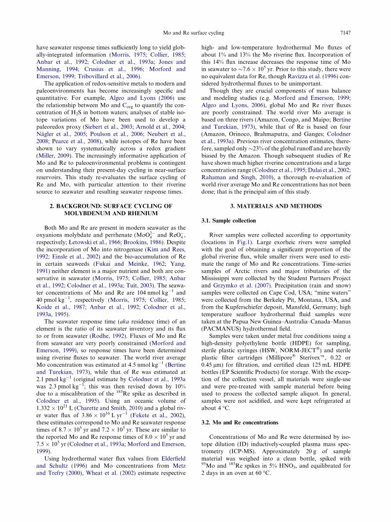
River samples were collected according to opportunity(locations in Fig.1). Large exorheic rivers were sampledwith the goal of obtaining a significant proportion of theglobal riverine flux, while smaller rivers were used to esti-mate the range of Mo and Re concentrations. Time-seriessamples of Arctic rivers and major tributaries of theMississippi were collected by the Student Partners Projectand Grzymko et al. (2007). Precipitation (rain and snow)samples were collected on Cape Cod, USA; “mine waters”

were collected from the Berkeley Pit, Montana, USA, andfrom the Kupferschiefer deposit, Mansfeld, Germany; hightemperature seafloor hydrothermal fluid samples weretaken at the Papua New Guinea–Australia–Canada–Manus(PACMANUS) hydrothermal field.

Samples were taken under metal free conditions using ahigh-density polyethylene bottle (HDPE) for sampling,sterile plastic syringes (HSW, NORM-JECT�) and sterileplastic filter cartridges (Millipore� Sterivexe, 0.22 or0.45 lm) for filtration, and certified clean 125 mL HDPEbottles (EP Scientific Products) for storage. With the excep-tion of the collection vessel, all materials were single-useand were pre-treated with sample material before beingused to process the collected sample aliquot. In general,samples were not acidified, and were kept refrigerated atabout 4 �C.

3.2. Mo and Re concentrations

Concentrations of Mo and Re were determined by iso-tope dilution (ID) inductively-coupled plasma mass spec-trometry (ICP-MS). Approximately 20 g of samplematerial was weighed into a clean bottle, spiked with95Mo and 185Re spikes in 5% HNO3, and equilibrated for2 days in an oven at 60 �C.

–90º

–45º

0º

45º

90º

–90º

–45º

0º

45º

90º

45º 0º 90º 135º ±180º –45º –90º –135º

±180º

12

3

5

10

11

12

13

14

15

1819

17

16

6

7

8

9

4

#

River

Precipitation

Mine water

Hydrothermal sample

Large-scale drainage region

Fig. 1. Locations for river, precipitation, mine water, and hydrothermal fluid samples analyzed for this study. Internally-draining continentalareas (i.e. non-exorheic) are hatched-out. Also shown are borders for the large-scale drainage regions (after Graham et al., 1999; data fromhttp://www.ngdc.noaa.gov/ecosys/cdroms/graham/graham/graham.htm#element7).

7148 C.A. Miller et al. / Geochimica et Cosmochimica Acta 75 (2011) 7146–7179

Chromatographic purification used 1 mL (wet volume)of pre-cleaned Biorad AG 1 � 8, 100–200 mesh anion resin(after Morgan et al., 1991). Chromatography was opti-mized for quantitative recovery of Re as Mo is typicallythree orders of magnitude more abundant in natural waters(Kharkar et al., 1968; Bertine and Turekian, 1973; Morris,1975; Collier, 1985; Anbar et al., 1992; Colodner et al.,1993a). Recovery of Mo, though not quantitative, was suf-ficient to obtain Mo ion beams larger than those of Re. AllMo and Re analyses were done with the ELEMENT 2 massspectrometer (Thermo Fisher Scientific) in the ICP-MSfacility. Samples were introduced using a perfluoroalkoxy(PFA) MicroFlow nebulizer (Elemental Scientific Incorpo-rated), a quartz spray chamber, and regular cones (Ni).Masses 95 (Mo), 97 (Mo), 98 (Mo), 185 (Re), 187 (Re),188 (Os), and 101 (Ru) were scanned 100 times in low massresolution; each nuclide was counted for a total of 2 s. Mass188 count rates were uniformly low, so no correction ismade for 187Os. Acid blanks and standards were analyzedevery five or six samples to correct for blank contributionsas well as instrumental mass fractionation using natural Moand Re isotopic ratios (Rosman and Taylor, 1998).

Uncertainties of Mo and Re concentration measure-ments were estimated using multiple (n = 12) analyses ofprocessed aliquots of a St. Lawrence sample from Coteaudu Lac, Quebec, Canada; Mo and Re uncertainties are6.2% and 4.6% (2 SD), respectively. This is similar to theRe concentration uncertainty of 4% reported by Colodneret al. (1993b).

3.3. Cation concentrations

Where feasible, concentrations of major (Na+, Mg2+,K+, Ca2+) and selected minor and trace cations (Rb+,Sr2+, and Ba2+) were determined by ID ICP-MS. Isotopedilution determination of Na was not possible as it ismono-isotopic; ID determination of K was complicatedby significant up-mass tailing of 40Ar on to 41K; ID

determination of both Rb and Sr would have doubled thenumber of analyses due to the isobars at mass 87. Concen-trations of Na, K, and Rb were determined by standard-calibration ICP-MS using 23Na, 39K, and 85Rb.

Sample aliquots of 1 mL were spiked with mixed25Mg–135Ba and 42Ca–84Sr, diluted 10-fold with 5% HNO3,and heated at 60 �C for 2 days to ensure spike-sampleequilibration. No purification chemistry was done.

Cation analyses were performed with the ELEMENT 2ICP-MS (Thermo Fisher Scientific) in the WHOI ICP-MSfacility. Samples were introduced using a PFA MicroFlownebulizer (Elemental Scientific Incorporated), a quartzspray chamber, and regular cones (Ni). Data were takenin low, medium, and high mass resolution. Low resolutionevaluated masses 23 (Na), 24 (Mg), 25 (Mg), 26 (Mg), 82(Kr), 83 (Kr), 84 (Kr + Sr), 85 (Rb), 86 (Kr + Sr), 87(Rb + Sr), 88 (Sr), 135 (Ba), 137 (Ba), and 138 (Ba); as withMo and Re, ion beam intensities are measured across 20channels of the central 5% of the peak. Medium resolutionevaluated masses 42 (Ca), 43 (Ca), 44 (Ca), and 48 (Ca) byintegrating the ion beam intensity of the entire peak. Highresolution evaluated masses 23 (Na), 24 (Mg), 25 (Mg), 26(Mg), and 39 (K) as whole peak integrations.

At the beginning of an analytical sequence, five-pointstandard calibration curves of 23Na, 39K, and 85Rb wereconstructed to evaluate these elements. Nuclide transmis-sion in the ELEMENT 2 is a function of mass and clo-sely follows a power law. Calibration curves were highlylinear (R2 > 0.99) across the counting-analog mode transi-tion of the secondary electron multiplier. The duration ofa typical analytical sequence (43 samples, 5 standards, 49rinse acid blanks) was �12 h. Standards evaluated duringand after a sequence indicated no significant instrumentaldrift.

As an internal consistency check, spike-unmixing of Mg,Ca, Sr, and Ba is done with multiple isotope ratios. 23So-dium was measured in both low and high resolution forthe same reason; unfortunately this was not done for K

Mo and Re surface cycling 7149

as proximity to the 40Ar peak restricts 39K acquisition tohigh resolution, or for Rb as even low-resolution 85Rb sig-nal intensities seldom exceeded 10 times the intensity in therinse acid blanks, preventing the acquisition of good data inmedium resolution.

Uncertainties were estimated using multiple samplealiquot processing (n = 22) and analyses (n = 33) of aSt. Lawrence sample from Coteau du Lac, Quebec, Canada.Uncertainties of Na, Mg, Ca, K, Rb, Sr, and Ba are 14%,1.3%, 10%, 16%, 15%, 20%, and 7% (2 SD) respectively.The uncertainty for Sr concentration is very large consider-ing analyses are done by ID; this is due to the �60% contri-bution of 84Kr to the mass 84 ion beam intensity.

3.4. Anion concentrations

Concentrations of Cl� and SO2�4 were determined

by standard-calibration using a Dionex� DX-500 ion

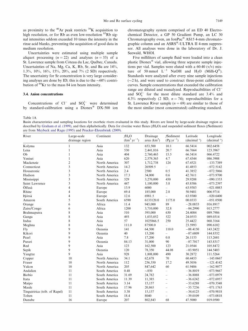
Table 1ABasin characteristics and sampling locations for exorheic rivers evaluatedescribed by Graham et al. (1999), and then alphabetically. Data for riveare from Meybeck and Ragu (1995) and Peucker-Ehrenbrink (2009).

River Large-scaledrainage region

Continent fH(k

Kolyma 1 Asia 13Lena 1 Asia 53Ob 1 Asia 40Yenisei 1 Asia 62Mackenzie 2 North America 30Connecticut 3 North America 14Housatonic 3 North America 2.Hudson 3 North America 17Mississippi 3 North America 52Saint Lawrence 3 North America 44Olfusa 4 Europe 13Rhine 4 Europe 69Þjorsa 4 Europe 12Amazon 5 South America 65Orange 6 Africa 11Zaire/Congo 6 Africa 12Brahmaputra 8 Asia 51Ganga 8 Asia 49Indus 8 Asia 57Meghna 8 Asia 11Fly 9 Oceania 14Kikori 9 Oceania 40Pearl 9 Asia 7.Purari 9 Oceania 84Red 9 Asia 12Sepik 9 Oceania 12Yangtze 9 Asia 92Copper 10 North America 34Fraser 10 North America 11Yukon 10 North America 20Andalien 11 South America 0.Biobıo 11 South America 31Itata 11 South America 11Maipo 11 South America 3.Maule 11 South America 17Tinguiririca (trib. of Rapel) 11 South America 5.Tolten 11 South America 18Danube 16 Europe 20

chromatography system comprised of an ED 40 Electro-chemical Detector, a GP 50 Gradient Pump, an LC 30Chromatography oven, an IonPac� AS15 4-mm chromato-graphic column and an ASRS�-ULTRA II 4-mm suppres-sor. All analyses were done in the laboratory of Dr. J.Seewald, WHOI.

Five milliliters of sample fluid were loaded into a cleanplastic Dionex� vial, allowing three separate sample injec-tions per vial. Samples were eluted with a 60:40 (v/v) mix-ture of 50 mmol L�1 NaOH and H2O (Milli-Q�).Standards were analyzed after every nine sample injections(�2 h), and were used to construct three-point calibrationcurves. Sample concentrations that exceeded the calibrationrange are diluted and reanalyzed. Reproducibilities of Cl�

and SO2�4 for the most dilute standard are 3.4% and

4.3% respectively (2 SD, n = 74); reproducibilities for aSt. Lawrence River sample (n = 69) are similar to those ofthe most similar (most concentrated) calibrating standard.

d in this study. Rivers are listed by large-scale drainage region asrine water fluxes (fH2O) and suspended sediment fluxes (fSediment)

2Om3 yr�1)

Drainagearea (km2)

fSediment(Pg yr�1)

Latitude(decimal �)

Longitude(decimal �)

2 653,500 10.1 66.5414 002.64580 2,441,816 20.7 66.7664 123.39674 2,760,465 15.5 66.5414 066.47220 2,579,365 4.7 67.4344 086.39087 1,712,738 124 67.4521 �133.7389.2 26509.5 – 41.4853 �072.51424 2500 0.5 41.3852 �072.5066.3 34,000 0.6 42.7611 �073.97009 3,270,000 450 29.9208 �090.13537 1,100,000 3.8 45.8586 �073.2397.9 6000 – 63.9383 �021.0083.4 185,000 2.8 50.9481 006.9714.6 6981.5 – 63.9300 �020.640090 6133120.0 1175.0 00.0333 �051.0500.4 945,000 89 �28.0833 016.891700 3,710,000 32.8 �04.2990 015.27770 595,000 630 24.4084 089.79863 1,033,052 522 24.0553 089.0314

1025866.5 250 25.4422 068.31641.0 87500.0 – 23.5993 090.61021 64,500 110.0 �08.4150 143.2422

13,200 – �07.6809 144.83528 17,200 0.8 26.1153 113.2681.13 31,000 90 �07.7017 143.83173 162,500 123 21.0544 105.84720 78,350 44.08 �03.9051 144.54038 1,808,000 490 30.2872 111.5264.1 62,678 70 60.4453 �145.06672 236,350 17.2 49.5056 �121.41425 847,642 60 61.9486 �162.907748 �850 – �36.8019 �073.9667.69 24,782 – �36.8088 �073.0979.39 11,385 – �36.6242 �072.695714 15,157 – �33.6288 �070.3548.96 20,865 – �35.7236 �071.176338 15,157 – �34.6125 �070.9818.4 8040 – �39.0109 �073.08187 802,843 68 47.5000 019.0500

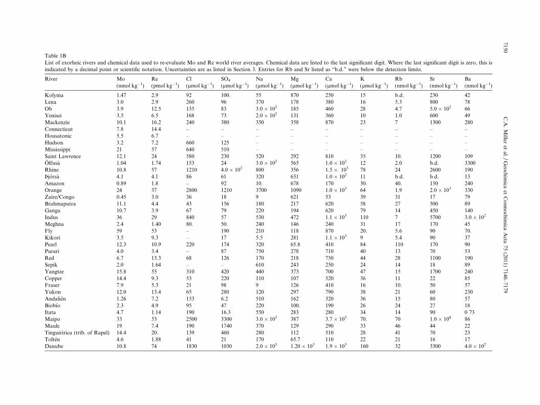
Table 1BList of exorheic rivers and chemical data used to re-evaluate Mo and Re world river averages. Chemical data are listed to the last significant digit. Where the last significant digit is zero, this isindicated by a decimal point or scientific notation. Uncertainties are as listed in Section 3. Entries for Rb and Sr listed as “b.d.” were below the detection limits.

River Mo(nmol kg�1)

Re(pmol kg�1)

Cl(lmol kg�1)

SO4

(lmol kg�1)Na(lmol kg�1)

Mg(lmol kg�1)

Ca(lmol kg�1)

K(lmol kg�1)

Rb(nmol kg�1)

Sr(nmol kg�1)

Ba(nmol kg�1)

Kolyma 1.47 2.9 92 100. 55 870 250 15 b.d. 230 42Lena 3.0 2.9 260 96 370 178 380 16 5.3 800 78Ob 3.9 12.5 135 83 3.0 � 102 185 460 28 4.7 5.0 � 102 66Yenisei 3.5 6.5 168 73 2.0 � 102 131 360 10 1.0 600 49Mackenzie 10.1 16.2 240 380 350 358 870 23 7 1300 280Connecticut 7.8 14.4 – – – – – – – – –Housatonic 5.5 6.7 – – – – – – – – –Hudson 3.2 7.2 660 125 – – – – – – –Mississippi 21 57 640 510 – – – – – – –Saint Lawrence 12.1 24 580 230 520 292 810 35 10. 1200 109Olfusa 1.04 1.74 153 24 3.0 � 102 565 1.0 � 102 12 2.0 b.d. 3300Rhine 10.8 57 1210 4.0 � 102 800 356 1.5 � 103 78 24 2600 190Þjorsa 4.1 4.1 86 61 320 631 1.0 � 102 11 b.d. b.d. 13Amazon 0.89 1.8 – 92 10. 678 170 30. 40. 150 240Orange 24 37 2800 1210 3700 1090 1.0 � 103 64 1.9 2.0 � 103 330Zaire/Congo 0.45 3.0 36 18 9 621 53 39 31 17 79Brahmaputra 11.1 4.4 43 156 180 217 620 58 27 500 89Ganga 10.7 3.9 67 79 220 194 620 79 14 450 140Indus 36 29 840 57 530 472 1.1 � 103 110 7 5700 3.0 � 102

Meghna 2.4 1.40 80. 50. 240 146 240 31 17 170 45Fly 59 53 – 190 210 118 870 20. 5.6 90 70.Kikori 3.5 9.3 – 17 5.5 281 1.1 � 103 9 5.4 90 37Pearl 12.3 10.9 220 174 320 65.8 410 84 110 170 90Purari 4.0 3.4 – 87 750 278 710 40 13 70 53Red 6.7 13.3 68 126 170 218 750 44 28 1100 190Sepik 2.0 1.64 – – 610 243 250 24 14 18 89Yangtze 15.8 55 310 420 440 373 700 47 15 1700 240Copper 14.4 9.3 53 220 110 107 520 36 11 22 85Fraser 7.9 5.3 21 98 9 126 410 16 10. 50 57Yukon 12.0 13.4 65 280 120 297 790 38 21 60 230Andalien 1.26 7.2 153 6.2 510 162 320 36 15 80 57Biobıo 2.3 4.9 95 47 220 100. 190 26 24 27 18Itata 4.7 1.14 190 16.3 550 283 280 34 14 90 0 73Maipo 33 53 2500 3300 3.0 � 102 387 3.7 � 103 70. 70 1.0 � 104 86Maule 19 7.4 190 1740 370 129 290 33 46 44 22Tinguiririca (trib. of Rapel) 14.4 20. 139 460 280 112 510 28 41 70 23Tolten 4.6 1.88 41 21 170 65.7 110 22 21 16 17Danube 10.8 74 1830 1030 2.0 � 103 1.20 � 103 1.9 � 103 160 32 3300 4.0 � 102

7150C

.A.

Miller

etal./

Geo

chim

icaet

Co

smo

chim

icaA

cta75

(2011)7146–7179

Table 2Mo, Re, and Mg chemical data for four hydrothermal fluid samples from the Roman Ruins vent site, PACMANUS, Manus Basin.

Vent orifice Mo(nmol kg�1)

Re(pmol kg�1)

Solutionmass (g)

Total Moa

(nmol)Total Rea

(pmol)Total Mo(nmol)

Total Re(pmol)

Mob

(nmol kg�1)Reb

(pmol kg�1)Mgc

(mmol kg�1)End-member Mod

(nmol kg�1)End-member Red

(pmol kg�1)

RMR 1 Fluide 4.3 1.5 750 3.2 1.1RMR 1 Dregs 640 72 25.769 16 1.9RMR 1 Bttl Fltrt 51 23 29.1013 2.1 0.94R RMR 1 21 4 29 5.3 8.7 10. �0.038RMR 2 Fluide 3.3 14.4 750 2.5 10.8RMR 2 Dregs 630 8.9 25.351 16 0.22RMR 2 Bttl Fltrt 82.2 97.4 29.1032 4.61 5.46R RMR 2 23 16 31 22 27 �27 5.6RMR 3 Fluide 3.7 0.65 750 2.8 0.48RMR 3 Dregs 180 10.8 111.933 20. 1.21RMR 3 Bttl Fltrt 49 12.7 28.4873 1.8 0.470R RMR 3 25 2 33 2.9 6.2 19 �0.92RMR 4 Fluide 14.9 0.82 750 11.2 0.61RMR 4 Dregs 1730 26 20.93 36.2 0.54RMR 4 Bttl Fltrt 111 12.5 28.9633 3.82 0.432R RMR 4 51 2 68 2.1 4.6 58 �0.69Bottom H2O 117.5 33 54.0

a For fluid and dregs subcomponents, total Mo and Re inventories are calculated by multiplying the concentrations and solution masses, however because the bottle filtrate fractions were notobtained from filtering the entire 750 g of fluid, the following scaling factors are applied to the bottle filtrate solution masses (the solution mass filtered is the denominator):

RMR 1: factor = 750 g/539.16 g = 1.3911,RMR 2: factor = 750 g/389.52 g = 1.9255,RMR 3: factor = 750 g/578.27 g = 1.2970,RMR 4: factor = 750 g/628.44 g = 1.1934.

b Calculated assuming an initial solution mass of 750 g.c Mg concentration data are from Craddock et al. (2010).d Calculated assuming bottom water Mg, Mo, and Re concentrations determined for the bottom water sample (“Bottom H2O”; see above).e Fluid samples were collected in August and September 2006 at approximately �3.7225�S, 151.6750�W. Temperature and pH (recalculated to 25 �C) listed below are from Craddock et al.

(2010).

RMR 1: T = 314 �C, pH = 2.4,RMR 2: T = 272 �C, pH = 2.7,RMR 3: T = 278 �C, pH = 2.5,RMR 4: T = 341 �C, pH = 2.6.

Mo

and

Re

surface

cycling

7151

Table 3AWater fluxes, water flux proportions, and average chemical concentrations for rivers of large-scale drainage region 1 (after Graham et al., 1999). The method of calculating flux-weighted regionalchemical averages used in this study is also shown.

Rivername

f H2Oð�1012 kg yr�1Þ

f H2Oa

(proportion)Individual river: chemical concentration averages

Mo (nmol kg�1) Re (pmol kg�1) Cl (lmol kg�1) SO4 (lmol kg�1) Na (lmol kg�1) Mg (lmol kg�1) Ca (lmol kg�1) K (lmol kg�1)

Kolyma 132 0.046 1.47 2.9 92 100. 55 87 250 15Lena 530 0.185 3.0 2.9 260 96 370 178 380 16Ob 404 0.141 3.9 12.5 135 83 3.0 � 102 185 460 28Yenisei 620 0.217 3.5 6.5 168 73 2.0 � 102 131 360 10.Rf H2O 1686 0.589

Individual river: annual chemical fluxes (i.e. ½X �river � f H2Oriver)b

nmol yr�1 � 1015 pmol yr�1 � 1014 lmol yr�1 � 1013 lmol yr�1 � 1013 lmol yr�1 � 1012 lmol yr�1 � 1013 lmol yr�1 � 1013 lmol yr�1 � 1012

Kolyma 1.94 3.8 1.2 1.33 7.2 1.2 3.3 2.0Lena 16 15 14 5.1 2.0 � 102 9.44 20. 8.2Ob 16 50.3 54.4 3.4 120 7.46 19 11Yenisei 22 40. 10.4 4.5 130 8.15 23 6.4

Rchemical fluxes 54.8 110. 30.7 14.3 450. 26.2 64.6 27.8

Large-scale drainage region: chemical concentration averages (i.e. Rchemical fluxes � Rf H2O)c

nmol kg�1 pmol kg�1 lmol kg�1 lmol kg�1 lmol kg�1 lmol kg�1 lmol kg�1 lmol kg�1

Region 1averages

3.3 6.5 182 85 270 155 380 16

a Proportions of H2O fluxes are the individual river fluxes divided by the regional sum (in this case, 2860.8 km3 yr�1 or 2860.8 � 1012 kg yr�1). Individual river fluxes are taken from thecompilation of Meybeck and Ragu (1995) while the large-scale drainage region 1 flux (after Graham et al., 1999) is from Peucker-Ehrenbrink (2009).

b Individual river chemical fluxes are obtained by multiplying the individual river chemical concentrations by the yearly riverine H2O fluxes.c Large-scale drainage region chemical concentration averages are obtained by taking the sum of the individual fluxes for the drainage region ðRchemical fluxesÞ, and dividing by the sum of the H2O

fluxes ðRf H2OÞ. The result is a flux-weighted chemical concentration for that portion of the large-scale drainage region that has been sampled (in this case 58.9% of the total regional H2O flux) thatis then applied to the water flux for the entire large-scale drainage region when determining global river average concentrations (see Table 3B).

7152C

.A.

Miller

etal./

Geo

chim

icaet

Co

smo

chim

icaA

cta75

(2011)7146–7179

Table 3BWater fluxes, water flux proportions, and average regional chemical concentrations for all large-scale drainage regions (after Graham et al., 1999) for which data are presented in this study.Resulting world river chemical concentrations are also shown.

Grahamregion

fH2O(km3 yr�1)

fH2Oa

(proportion)Large-scale drainage region chemical concentration averagesb

Mo (nmol kg�1) Re (pmol kg�1) Cl (lmol kg�1) SO4 (lmol kg�1) Na (lmol kg�1) Mg (lmol kg�1) Ca (lmol kg�1) K (lmol kg�1)

1 2855.8 0.082 3.2 6.5 182 85 270 155 380 162 846.1 0.024 10.1 16.2 240 380 350 358 870 233 2687.8 0.077 16.5 41 6.0 � 102 380 5.0 � 102 282 780 344 821.7 0.024 8.5 42 910 3.0 � 102 670 274 1100 605 10898.6 0.313 0.89 1.83 – 92 1.0 � 102 67.8 160 306 2426.9 0.070 0.68 3.3 63 29 120 71.8 62 40.8 4050.7 0.116 11.3 5.1 95 134 220 213 6.0 � 102 70.9 7001.3 0.201 17.0 42 283 330 410 314 690 4110 1688.3 0.049 10.9 10.4 50. 220 110 224 640 3111 1128.5 0.032 8.4 7.0 2.0 � 102 2.0 � 102 380 133 350 2916 403.5 0.012 10.8 74 1830 1030 2.0 � 103 1200 1900 160

Global River Averagec 8.0 16.5 190 190 270 193 470 38

a Proportions of H2O fluxes are the individual regional fluxes divided by their sum (34,809 km3 yr�1). Note that though we do not have samples for regions 7, 12, 13, 14, 15, 17, 18, and 19, thesum of the H2O fluxes for the regions sampled for this study is �90% of the total exorheic H2O flux.

b The method by which regional chemical averages are calculated is shown in detail in Table 3A.c The global chemical averages are calculated in the same manner as the regional averages (see Table 3A). The regional chemical flux contributions are calculated, then summed and divided by

the sum of the regional H2O fluxes.

Mo

and

Re

surface

cycling

7153

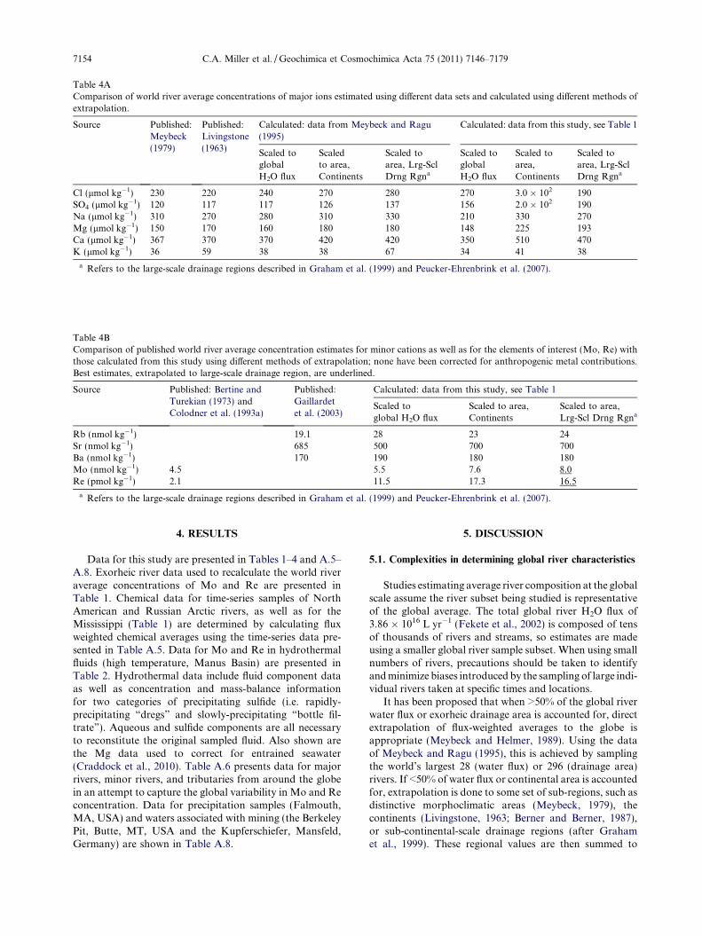
Table 4AComparison of world river average concentrations of major ions estimated using different data sets and calculated using different methods ofextrapolation.

Source Published:Meybeck(1979)

Published:Livingstone(1963)

Calculated: data from Meybeck and Ragu(1995)

Calculated: data from this study, see Table 1

Scaled toglobalH2O flux

Scaledto area,Continents

Scaled toarea, Lrg-SclDrng Rgna

Scaled toglobalH2O flux

Scaled toarea,Continents

Scaled toarea, Lrg-SclDrng Rgna

Cl (lmol kg�1) 230 220 240 270 280 270 3.0 � 102 190SO4 (lmol kg�1) 120 117 117 126 137 156 2.0 � 102 190Na (lmol kg�1) 310 270 280 310 330 210 330 270Mg (lmol kg�1) 150 170 160 180 180 148 225 193Ca (lmol kg�1) 367 370 370 420 420 350 510 470K (lmol kg�1) 36 59 38 38 67 34 41 38

a Refers to the large-scale drainage regions described in Graham et al. (1999) and Peucker-Ehrenbrink et al. (2007).

Table 4BComparison of published world river average concentration estimates for minor cations as well as for the elements of interest (Mo, Re) withthose calculated from this study using different methods of extrapolation; none have been corrected for anthropogenic metal contributions.Best estimates, extrapolated to large-scale drainage region, are underlined.

Source Published: Bertine andTurekian (1973) andColodner et al. (1993a)

Published:Gaillardetet al. (2003)

Calculated: data from this study, see Table 1

Scaled toglobal H2O flux

Scaled to area,Continents

Scaled to area,Lrg-Scl Drng Rgna

Rb (nmol kg�1) 19.1 28 23 24Sr (nmol kg�1) 685 500 700 700Ba (nmol kg�1) 170 190 180 180Mo (nmol kg�1) 4.5 5.5 7.6 8.0Re (pmol kg�1) 2.1 11.5 17.3 16.5

a Refers to the large-scale drainage regions described in Graham et al. (1999) and Peucker-Ehrenbrink et al. (2007).

7154 C.A. Miller et al. / Geochimica et Cosmochimica Acta 75 (2011) 7146–7179

4. RESULTS

Data for this study are presented in Tables 1–4 and A.5–A.8. Exorheic river data used to recalculate the world riveraverage concentrations of Mo and Re are presented inTable 1. Chemical data for time-series samples of NorthAmerican and Russian Arctic rivers, as well as for theMississippi (Table 1) are determined by calculating fluxweighted chemical averages using the time-series data pre-sented in Table A.5. Data for Mo and Re in hydrothermalfluids (high temperature, Manus Basin) are presented inTable 2. Hydrothermal data include fluid component dataas well as concentration and mass-balance informationfor two categories of precipitating sulfide (i.e. rapidly-precipitating “dregs” and slowly-precipitating “bottle fil-trate”). Aqueous and sulfide components are all necessaryto reconstitute the original sampled fluid. Also shown arethe Mg data used to correct for entrained seawater(Craddock et al., 2010). Table A.6 presents data for majorrivers, minor rivers, and tributaries from around the globein an attempt to capture the global variability in Mo and Reconcentration. Data for precipitation samples (Falmouth,MA, USA) and waters associated with mining (the BerkeleyPit, Butte, MT, USA and the Kupferschiefer, Mansfeld,Germany) are shown in Table A.8.

5. DISCUSSION

5.1. Complexities in determining global river characteristics

Studies estimating average river composition at the globalscale assume the river subset being studied is representativeof the global average. The total global river H2O flux of3.86 � 1016 L yr�1 (Fekete et al., 2002) is composed of tensof thousands of rivers and streams, so estimates are madeusing a smaller global river sample subset. When using smallnumbers of rivers, precautions should be taken to identifyand minimize biases introduced by the sampling of large indi-vidual rivers taken at specific times and locations.

It has been proposed that when >50% of the global riverwater flux or exorheic drainage area is accounted for, directextrapolation of flux-weighted averages to the globe isappropriate (Meybeck and Helmer, 1989). Using the dataof Meybeck and Ragu (1995), this is achieved by samplingthe world’s largest 28 (water flux) or 296 (drainage area)rivers. If <50% of water flux or continental area is accountedfor, extrapolation is done to some set of sub-regions, such asdistinctive morphoclimatic areas (Meybeck, 1979), thecontinents (Livingstone, 1963; Berner and Berner, 1987),or sub-continental-scale drainage regions (after Grahamet al., 1999). These regional values are then summed to

Calendar date, 2004Jul 1 May 1Mar 1Jan 1

H2O

flux

, km

3 d-1

; Mo,

nm

ol k

g-1

Daily M

o flux, % of total

0

2

4

6

8

10

0

0.2

0.4

0.6

0.8

1.0

Sep 1 Nov 1 Dec 31

daily H2O flux

H2O flux wtd annual Mo river average

Mo concentration daily Mo flux

Fig. 2. Fluxes of H2O and Mo, as well as Mo concentrations forthe Yenisei River, 2004. Water flux data are from http://rims.unh.edu/ (see footnotes, Table A.5). Intervals between Momeasurements are interpolated linearly (point-to-point). Daily Mofluxes are the product of daily H2O fluxes and interpolated ormeasured Mo concentrations. These daily fluxes are summed anddivided by the yearly H2O flux to determine flux-weighted yearlyaverage Mo concentration (dashed line).

Mo and Re surface cycling 7155

account for global runoff. If possible, rivers should besampled in an attempt to capture the large inter-river vari-ability caused by differences in basin morphology, climate,and geology.

There is also significant intra-river variability; one sam-pling event represents a single snapshot of the river in timeand space, and a temporal–spatial integration of the rivershould therefore be attempted where possible. Obtainingspatially integrated samples is theoretically simple; samplesobtained at the river mouth are representative of the entiredrainage region. Truly reliable averages for a single rivershould be obtained with time-series measurements thatare then flux-weighted to give a yearly average (Living-stone, 1963; Meybeck and Helmer, 1989). Though this isdesirable, the number of rivers required to provide largeproportions of total water flux renders it impractical.

In many cases, even monthly surveys may not be suffi-cient (Livingstone, 1963). Fig. 2 shows the 2004 water fluxfor the Yenisei River (see also Table A.5). The large H2Opulse associated with the spring freshet accounts for�40% of the yearly H2O flux over the course of 1 month(�8% of the year). In the case of large Arctic rivers suchas the Yenisei, the freshet must be sampled.

Because of the difficulty of obtaining river samples forspecific locations and times, many samples are samples ofopportunity. For example, significant tributaries are some-times assumed to represent the main stem of a river. In thisstudy only one of the exorheic rivers presented in Table 1 isrepresented by a single major tributary (the Tinguiririca is atributary of the Rapel).

5.2. Calculation of present-day average Mo and Re

concentrations in rivers

Prior estimates of world river Mo and Re averages usedsample subsets of three rivers (Amazon, Congo, Maipo)

and four rivers (Amazon, Orinoco, Ganges, Brahmaputra),respectively (Bertine and Turekian, 1973; Colodner et al.,1993a). Using global flux and exorheic land area data fromFekete et al. (2002) and Peucker-Ehrenbrink et al. (2007),these subsets account for 22% (Mo) and 24% (Re) of thewater flux and 7.6% (Mo) and 6.6% (Re) of exorheic conti-nental area. Though these limited sample sets seeminglynecessitate extrapolation to some larger global sub-region,such attempts are meaningless as so few of these regionsare characterized. These early investigations extrapolate di-rectly to the global river water flux.

This study analyzes 38 exorheic rivers (Table 1), encom-passing 37% of total water runoff and 22% of total exorheicdrainage area. This larger more geographically varied sam-ple set allows the regional extrapolation not attempted forprevious estimates. In this study, we favor the 19 large-scaledrainage regions of Graham et al. (1999) rather than the 14morphoclimatic zones of Meybeck (1979) or the total con-tinental areas used by Livingstone (1963). The large-scaledrainage regions are delineated according to continentalrunoff into specific regions of the world ocean or large in-land seas, and are a useful subdivision of global drainagearea as they form part of a river transport algorithm de-signed for climate modeling (Graham et al., 1999), and be-cause they have been characterized in terms of bedrockgeology (Peucker-Ehrenbrink et al., 2007). Table 3 liststhe large-scale drainage areas for which data are presentedin this study.

The potential for bias introduced by our calculationmethod is evaluated in Table 4A, using published major ele-mental concentration data from the compilation ofMeybeck and Ragu (1995, �250 rivers, 60% global H2Oflux, 51% global drainage area). World river averages calcu-lated with this compilation agree well with the publishedvalues of Meybeck (1979) and Livingstone (1963). Calcu-lated Meybeck and Ragu (1995) averages also agree wellacross the different calculation methods for all major anionsand cations except K. This generally good agreement is tobe expected for a data set accounting for such a large pro-portion of global totals. Results from the same calculationsusing data from Table 1 show good agreement with pub-lished values of Na, Mg, K, and Cl, but are somewhathigher for Ca, and SO4. As expected for a much smallersample set, averages calculated from Table 1 data showlarger variations across the different calculation methods.Likewise, published Rb, Sr, and Ba averages (Gaillardetet al., 2003, �36 rivers, 37% global H2O, flux, 33% globaldrainage area), are very similar to those calculated fromTable 1 data. Consideration of the river averages calculatedfor major and minor ions indicates that our sub-sample setis broadly consistent with global river chemistry and cantherefore be used to re-calculate the world river averageconcentrations of Mo and Re. The results of these calcula-tions are presented in Table 4B.

Recalculated Mo and Re world river averages arerespectively two and eight times greater than previous esti-mates (Bertine and Turekian, 1973; Colodner et al., 1993a).Significant changes are not surprising given that the smallnumbers of rivers evaluated for previous estimates intro-duces the possibility of significant bias. For example,

7156 C.A. Miller et al. / Geochimica et Cosmochimica Acta 75 (2011) 7146–7179

despite being only �17% of the global river H2O flux, theAmazon accounts for 76% and 85% of total H2O fluxesused in previous estimates. Because the Amazon has lowMo and Re concentrations, this bias is seen in the world riv-er averages calculated according to different methods in thisstudy (Table 4B). The Amazon represents nearly half of the�37% of the global river H2O flux accounted for by the riv-ers in Table 1; averages calculated by simply scaling to theglobal H2O flux are, therefore, lower than those obtainedby first scaling to the continental area or large-scale drain-age region in which the proportional water flux of theAmazon is kept closer to its global value.

Using modern Mo and Re average river concentrationsof 8.0 nmol kg�1 and 16.5 pmol kg�1 (Table 3B) and a glo-bal river H2O flux of 3.86 � 1016 kg yr�1 (Fekete et al.,2002), modern fluxes of these metals to seawater are3.1 � 108 mol yr�1 (Mo) and 6.4 � 105 mol yr�1 (Re). Inthe following sections, we evaluate natural and anthropo-genic sources of Mo and Re to world rivers.

5.3. Anthropogenic contributions and the pre-anthropogenic

world river average of Re

Industrial production of Mo and Re introduces ananthropogenic component to their modern surface cycles.The potential for a pollutive contribution to Mo was recog-nized by Bertine and Turekian (1973) and accounts for theirdecision to estimate an average river concentration basedon rivers from the southern hemisphere. Likewise, Manheimand Landergren (1978) used analyses of “pristine” Arcticrivers to estimate that modern Mo fluxes are twice thepre-anthropogenic value. Similarly, Colodner et al. (1995)and Rahaman and Singh (2010) invoke anthropogeniccontamination to explain the elevated Re concentrations ofrivers draining into the Black Sea and the Gulf of Cambay,respectively.

Anthropogenically-enhanced delivery of Mo and Re tomodern oceans is expected on the basis of the high concen-trations of these metals in fossil fuels (Bertine andGoldberg, 1971; Poplavko et al., 1974; Duyck et al., 2002;Selby et al., 2005, 2007a), and their presence in fuel process-ing catalysts (Chang, 1998; Moyse, 2000). Furthermore, theuse of Re in brake liners is thought to be the source for highconcentrations of Re (up to 10 ng g�1) in road dusts (Meiseland Stotter, 2007).

Table A.8 contains data for precipitation samples fromFalmouth, MA, USA. Many of these samples containnon-negligible metal concentrations even after correctingfor cyclic sea salt. Concentrations of Mo are consistentwith, though generally lower than, those reported forJapanese rain samples (Sugawara et al., 1961). These arethe first data for Re in precipitation, and the unexpectedlyhigh concentrations of some samples (e.g. 5.9 pmol Re kg�1)may be evidence of an atmospheric anthropogenic Recomponent as hypothesized by Chappaz et al. (2008).

Previous studies noted the likelihood of anthropogenicRe contamination in rivers (Colodner et al., 1995; Rahamanand Singh, 2010), and major rivers evaluated for this study(Table 1) may support this, as many known to exhibitanthropogenic effects also have high metal concentrations

(Danube, Mississippi, Rhine, Yangtze). Quantifying the ef-fects of anthropogenic contamination is difficult because ofwide natural variations and a lack of pre-industrial riversamples. Where such samples do exist, they illustrate a largeanthropogenic influence on river chemistry (e.g. a 4-fold in-crease for dissolved SO2�

4 and a 13-fold increase for dis-solved Cl� in the Rhine between 1854 and 1981; Zobristand Stumm, 1981).

Some samples evaluated in this study exhibit unambigu-ous anthropogenic contamination by virtue of their extre-mely elevated Re concentrations. The highest riverconcentration, 1240 pmol Re kg�1 for a sample of the SouthPlatte river (Table A.6B), is likely due to evaporative concen-tration of Re in groundwater used for irrigation. Groundwa-ter irrigation was observed in the area at the time ofsampling, and groundwaters exhibit higher concentrationsof Re than our world average (Hodge et al., 1996; Leybourneand Cameron, 2008). In addition, a sample of the SouthPlatte from much closer to the headwaters (at 11 MileCanyon) has a much lower Re concentration (37 pmol kg�1;Table A.6B). Table A.8 contains data for water samples frommining areas (Berkeley Pit from Butte, MT, USA andKupferschiefer from Mansfeld, Germany). Concentrationsof Re in these samples (11,900–37,000 pmol kg�1) are thehighest observed for water samples, with enrichment factorsof 700–2200 times the average river concentration deter-mined in this study. These samples have concentrationsequivalent to or higher than estimates of Re in thecrust (Esser and Turekian, 1993; Hauri and Hart, 1997;Peucker-Ehrenbrink and Jahn, 2001; Sun et al., 2003a). Con-centrations of Mo in these samples do not display the samelevel of enrichment; Mansfeld samples show concentrationsranging from 190 to 250 nmol Mo kg�1 (23–32 times worldriver average), Berkeley Pit samples have Mo concentrationsof less than 1 nmol kg�1 (�0.08 times the world riveraverage). The extremely high Re enrichments but only lowto moderately high Mo enrichments in waters associatedwith mining suggests that Re may be a particularly sensitivetracer of anthropogenic heavy metal contamination.

Given the compelling evidence for anthropogenic Re con-tamination, it should be quantified in order to determine thepre-anthropogenic river average. The linear relationship ob-served between Re and SO2�

4 in rivers (Section 5.4, Fig. 3;Colodner et al., 1993a; Dalai et al., 2002) allows us to do this.The anthropogenic SO2�

4 contribution of world rivers is var-iably estimated at 28% (Berner, 1971; Meybeck, 1979), 32%(Meybeck, 1988), and 43% (Berner and Berner, 1987). Themagnitudes of anthropogenic corrections of global river Reconcentration depend on the choice of both average SO2�

4

concentration and anthropogenic SO2�4 contribution. Using:

(i) SO2�4 river concentration estimates of Meybeck (1979) and

Livingstone (1963), and (ii) anthropogenic SO2�4 estimates

from the literature (Berner, 1971; Berner and Berner,1987), (iii) SO2�

4 estimates from Table 4A, as well as (iv)pristine river SO2�

4 concentration estimates (81.5 lmolSO2�

4 kg�1; Meybeck and Helmer, 1989), we obtainpre-anthropogenic world river Re concentrations rangingfrom 6.5 to 11.9 pmol kg�1.

Our best-estimate for anthropogenically-corrected aver-age river Re concentration is 11.2 pmol kg�1. The estimate

10-110-2

10 0

10 2

10 4

10 6

10 8

10 10

10 1 10 3 10 5 10 7 10 9

SO422- or S, μmol kg -1

Re,

pm

ol k

g,

- 1

Riverv

Precipitatione

Berkeley PitB k l Pite

UCCCSeawatere

Groundwatero r

Black shalea

MoSo 2 hist.

‘FeSS22’ hist.his

y = 0.100y x

R2 = 0.76=

porphyry Cuuu,Chilee

GGGGrrrrrrreat Basin,e iUSA

ReSe 2

porphyry Cu,,ChileChil

H 2O – ReSS22 m

ixing line

m22

Great Basin,BUSAAA

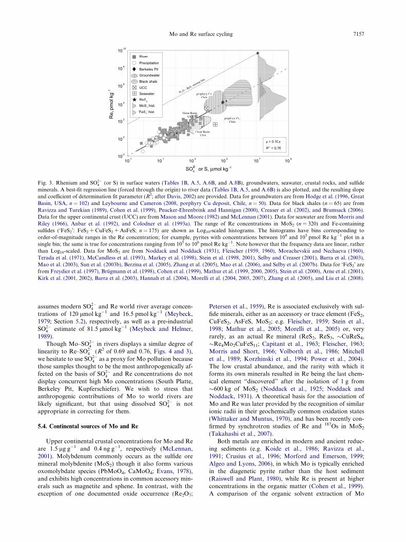
Fig. 3. Rhenium and SO2�4 (or S) in surface waters (Tables 1B, A.5, A.6B, and A.8B), groundwaters, seawater, crustal rocks, and sulfide

minerals. A best-fit regression line (forced through the origin) to river data (Tables 1B, A.5, and A.6B) is also plotted, and the resulting slopeand coefficient of determination fit parameter (R2; after Davis, 2002) are provided. Data for groundwaters are from Hodge et al. (1996, GreatBasin, USA, n = 102) and Leybourne and Cameron (2008, porphyry Cu deposit, Chile, n = 50). Data for black shales (n = 65) are fromRavizza and Turekian (1989), Cohen et al. (1999), Peucker-Ehrenbrink and Hannigan (2000), Creaser et al. (2002), and Brumsack (2006).Data for the upper continental crust (UCC) are from Mason and Moore (1982) and McLennan (2001). Data for seawater are from Morris andRiley (1966), Anbar et al. (1992), and Colodner et al. (1993a). The range of Re concentrations in MoS2 (n = 320) and Fe-containingsulfides (‘FeS2’: FeS2 + CuFeS2 + AsFeS; n = 175) are shown as Log10-scaled histograms. The histograms have bins corresponding toorder-of-magnitude ranges in the Re concentration; for example, pyrites with concentrations between 104 and 105 pmol Re kg�1 plot in asingle bin; the same is true for concentrations ranging from 105 to 106 pmol Re kg�1. Note however that the frequency data are linear, ratherthan Log10-scaled. Data for MoS2 are from Noddack and Noddack (1931), Fleischer (1959, 1960), Morachevskii and Nechaeva (1960),Terada et al. (1971), McCandless et al. (1993), Markey et al. (1998), Stein et al. (1998, 2001), Selby and Creaser (2001), Barra et al. (2003),Mao et al. (2003), Sun et al. (2003b), Berzina et al. (2005), Zhang et al. (2005), Mao et al. (2006), and Selby et al. (2007b). Data for ‘FeS2’ arefrom Freydier et al. (1997), Brugmann et al. (1998), Cohen et al. (1999), Mathur et al. (1999, 2000, 2005), Stein et al. (2000), Arne et al. (2001),Kirk et al. (2001, 2002), Barra et al. (2003), Hannah et al. (2004), Morelli et al. (2004, 2005, 2007), Zhang et al. (2005), and Liu et al. (2008).

Mo and Re surface cycling 7157

assumes modern SO2�4 and Re world river average concen-

trations of 120 lmol kg�1 and 16.5 pmol kg�1 (Meybeck,1979; Section 5.2), respectively, as well as a pre-industrialSO2�

4 estimate of 81.5 lmol kg�1 (Meybeck and Helmer,1989).

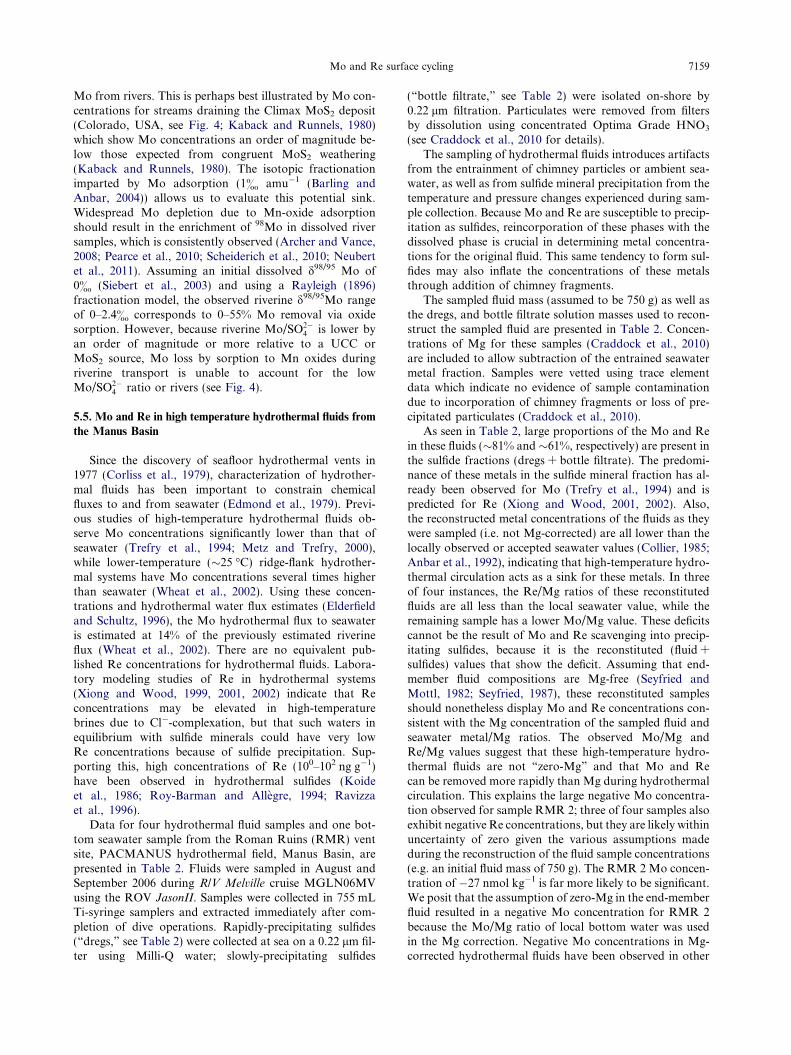
Though Mo–SO2�4 in rivers displays a similar degree of

linearity to Re–SO2�4 (R2 of 0.69 and 0.76, Figs. 4 and 3),

we hesitate to use SO2�4 as a proxy for Mo pollution because

those samples thought to be the most anthropogenically af-fected on the basis of SO2�

4 and Re concentrations do notdisplay concurrent high Mo concentrations (South Platte,Berkeley Pit, Kupferschiefer). We wish to stress thatanthropogenic contributions of Mo to world rivers arelikely significant, but that using dissolved SO2�

4 is notappropriate in correcting for them.

5.4. Continental sources of Mo and Re

Upper continental crustal concentrations for Mo and Reare 1.5 lg g�1 and 0.4 ng g�1, respectively (McLennan,2001). Molybdenum commonly occurs as the sulfide oremineral molybdenite (MoS2) though it also forms variousoxomolybdate species (PbMoO4, CaMoO4; Evans, 1978),and exhibits high concentrations in common accessory min-erals such as magnetite and sphene. In contrast, with theexception of one documented oxide occurrence (Re2O7;

Petersen et al., 1959), Re is associated exclusively with sul-fide minerals, either as an accessory or trace element (FeS2,CuFeS2, AsFeS, MoS2; e.g. Fleischer, 1959; Stein et al.,1998; Mathur et al., 2005; Morelli et al., 2005) or, veryrarely, as an actual Re mineral (ReS2, ReS3, �CuReS4,�Re4Mo2CuFeS11; Capitant et al., 1963; Fleischer, 1963;Morris and Short, 1966; Volborth et al., 1986; Mitchellet al., 1989; Korzhinski et al., 1994; Power et al., 2004).The low crustal abundance, and the rarity with which itforms its own minerals resulted in Re being the last chem-ical element “discovered” after the isolation of 1 g from�600 kg of MoS2 (Noddack et al., 1925; Noddack andNoddack, 1931). A theoretical basis for the association ofMo and Re was later provided by the recognition of similarionic radii in their geochemically common oxidation states(Whittaker and Muntus, 1970), and has been recently con-firmed by synchrotron studies of Re and 187Os in MoS2

(Takahashi et al., 2007).Both metals are enriched in modern and ancient reduc-

ing sediments (e.g. Koide et al., 1986; Ravizza et al.,1991; Crusius et al., 1996; Morford and Emerson, 1999;Algeo and Lyons, 2006), in which Mo is typically enrichedin the diagenetic pyrite rather than the host sediment(Raiswell and Plant, 1980), while Re is present at higherconcentrations in the organic matter (Cohen et al., 1999).A comparison of the organic solvent extraction of Mo

10- 110- 2

10 0

10 2

10 4

10 6

10 8

10 10

10 1 10 3 10 5 10 7 10 9

Mo,

nm

ol k

g - 1

SO42 - or S, μmol kg- 1

River

Precipitation

Berkeley Pit

UCCSeawater

Groundwater

Anoxic seds.

MoS2

y = 0.0089x

R2 = 0.69

porphyry Cu,Chile

H 2O – MoS 2

mixing lin

e

Great Basin,USA

MoS2 streamsFeS2 hist.

Fig. 4. Molybdenum and SO2�4 (or S) in surface waters (Tables 1B, A.5, A.6B, and A.8B), groundwaters, seawater, crustal rocks, and sulfides

(FeS2, MoS2). A best-fit regression line (forced through the origin) to river data (Tables 1B, A.5, and A.6B) is also plotted, and the resultingslope and coefficient of determination fit parameter (R2; after Davis, 2002) are provided. A mixing line between MoS2 and a hypothetical“pure” water (zero-SO2�

4 , zero-Mo) is also shown. Data for groundwaters are from Hodge et al. (1996, Great Basin, USA, n = 84) andLeybourne and Cameron (2008, porphyry Cu deposit, Chile, n = 50). Data for black shales and Black Sea sediments (“Anoxic seds.,” n = 281)are from Breger and Schopf (1955), Le Riche (1959), Wedepohl (1964), Vine et al. (1969), Hirst (1974), Pilipchuk and Volkov (1974), Lipinskiet al. (2003), Brumsack (2006), Chaillou et al. (2008), and Hetzel et al. (2009). Data for the upper continental crust (UCC) are from Masonand Moore (1982) and McLennan (2001). Data for seawater are from Morris and Riley (1966), Morris (1975), and Collier (1985). Data forstreams draining the Climax Mo mine, Colorado (“MoS2 streams,” n = 2), are from Kaback and Runnels (1980). Data for the range ofMo concentrations in FeS2 (n = 314) are shown as a smoothed Log10-scaled histogram. The histogram has bins that correspond to anorder-of-magnitude range in the Mo concentration; for example, pyrites with concentrations between 104 and 105 nmol Mo kg�1 plot in asingle bin; the same is true for concentrations ranging from 105 to 106 nmol Mo kg�1. Note however that the frequency data are linear, ratherthan Log10-scaled. Data are from Le Riche (1959), Badalov et al. (1966), Manheim (1972), Manheim and Siems (1972), Volkov and Fomina(1974), Raiswell and Plant (1980), Patterson et al. (1986), Huerta-Diaz and Morse (1992), Huston et al. (1995), Nesheim et al. (1997), Spearset al. (1999), Zhang et al. (2002), Tuttle et al. (2003, 2009), Tribovillard et al. (2008), Large et al. (2009), and Maslennikov et al. (2009).

7158 C.A. Miller et al. / Geochimica et Cosmochimica Acta 75 (2011) 7146–7179

and Re indicates that a significant proportion of Re, butnot Mo, is organically-bound, perhaps as metalloporphyrinspecies (Miller, 2004).

The association of Re, Mo, and S as sulfides in the crustand the high solubilities of their oxidized species MoO2�

4 ,ReO�4 , and SO2�

4 implies the effective mobilization of theseelements by oxidative weathering and suggests an associa-tion in the dissolved phase as seen in Figs. 3 and 4. The lin-earity of dissolved Re and SO2�

4 , previously observed forthe individual rivers (Colodner et al., 1993a; Dalai et al.,2002), can now be extended globally.

The Re–SO2�4 relationship in river samples is consistent

with precipitation samples, reported groundwater data(Hodge et al., 1996; Leybourne and Cameron, 2008) as wellas proposed Re and S concentrations for upper continentalcrust (UCC) and black shale sources (Fig. 3). In contrast,the Mo–SO2�

4 relationship of rivers is consistent with nei-ther the UCC and black shale abundances, nor with thecongruent weathering of MoS2 (Fig. 4). Relative to thesepresumed sources, rivers exhibit an excess of SO2�

4 , a deficitof Mo, or some combination of the two. The differences inthe Mo/SO2�

4 of rivers, UCC, and MoS2 are illustrative ofthe Mo riverine source.

Molybdenum concentrations in FeS2 (Fig. 4) suggestthat modern river concentrations of Mo are consistent witha predominantly pyritic continental source. Sources withhigher Mo/S ratios, such as UCC and black shales, must

be either less susceptible to weathering or volumetricallyunimportant. Likewise, due to the rarity of ReS2, weather-ing of this mineral cannot be a significant source of Re torivers. It should be noted that the observed riverineRe/SO2�

4 correlation is consistent with some mixture ofMoS2 and Fe-containing sulfides as the dominant weather-ing source.

The discrepancy between riverine and UCC Mo/SO2�4

might also be caused by sulfate weathering, but we do notthink this is likely. Riverine Re/SO2�

4 ratio is consistentwith that of UCC, while for Mo/SO2�

4 it is much lower.To be consistent with rivers and the UCC, sulfate mineralswould need Re concentrations of �120 ng Re g�1 (100-foldhigher than the UCC average). Though we have not foundpublished data for Re in sulfate or evaporite minerals, weconsider such high concentrations improbable. Thecorresponding gypsum-anhydrite concentration of Mo,�6 lg g�1, is of the same order as the UCC Mo average(McLennan, 2001). The range shown by the few publisheddata on sulfate Mo concentrations (10 lg g�1 and60 ng g�1; Manheim and Siems, 1972; Neubert et al.,2011) encompass this value, but we believe the requiredde-coupling of Re and Mo during weathering and the like-lihood of a pyrite Mo source render a significant continen-tal sulfate source unlikely.

Finally, the difference between riverine and UCCMo/SO2�

4 ratios might be due to sorptive loss of weathered

Mo and Re surface cycling 7159

Mo from rivers. This is perhaps best illustrated by Mo con-centrations for streams draining the Climax MoS2 deposit(Colorado, USA, see Fig. 4; Kaback and Runnels, 1980)which show Mo concentrations an order of magnitude be-low those expected from congruent MoS2 weathering(Kaback and Runnels, 1980). The isotopic fractionationimparted by Mo adsorption (1& amu�1 (Barling andAnbar, 2004)) allows us to evaluate this potential sink.Widespread Mo depletion due to Mn-oxide adsorptionshould result in the enrichment of 98Mo in dissolved riversamples, which is consistently observed (Archer and Vance,2008; Pearce et al., 2010; Scheiderich et al., 2010; Neubertet al., 2011). Assuming an initial dissolved d98/95 Mo of0& (Siebert et al., 2003) and using a Rayleigh (1896)fractionation model, the observed riverine d98/95Mo rangeof 0–2.4& corresponds to 0–55% Mo removal via oxidesorption. However, because riverine Mo/SO2�

4 is lower byan order of magnitude or more relative to a UCC orMoS2 source, Mo loss by sorption to Mn oxides duringriverine transport is unable to account for the lowMo/SO2�

4 ratio or rivers (see Fig. 4).

5.5. Mo and Re in high temperature hydrothermal fluids from

the Manus Basin

Since the discovery of seafloor hydrothermal vents in1977 (Corliss et al., 1979), characterization of hydrother-mal fluids has been important to constrain chemicalfluxes to and from seawater (Edmond et al., 1979). Previ-ous studies of high-temperature hydrothermal fluids ob-serve Mo concentrations significantly lower than that ofseawater (Trefry et al., 1994; Metz and Trefry, 2000),while lower-temperature (�25 �C) ridge-flank hydrother-mal systems have Mo concentrations several times higherthan seawater (Wheat et al., 2002). Using these concen-trations and hydrothermal water flux estimates (Elderfieldand Schultz, 1996), the Mo hydrothermal flux to seawateris estimated at 14% of the previously estimated riverineflux (Wheat et al., 2002). There are no equivalent pub-lished Re concentrations for hydrothermal fluids. Labora-tory modeling studies of Re in hydrothermal systems(Xiong and Wood, 1999, 2001, 2002) indicate that Reconcentrations may be elevated in high-temperaturebrines due to Cl�-complexation, but that such waters inequilibrium with sulfide minerals could have very lowRe concentrations because of sulfide precipitation. Sup-porting this, high concentrations of Re (100–102 ng g�1)have been observed in hydrothermal sulfides (Koideet al., 1986; Roy-Barman and Allegre, 1994; Ravizzaet al., 1996).

Data for four hydrothermal fluid samples and one bot-tom seawater sample from the Roman Ruins (RMR) ventsite, PACMANUS hydrothermal field, Manus Basin, arepresented in Table 2. Fluids were sampled in August andSeptember 2006 during R/V Melville cruise MGLN06MVusing the ROV JasonII. Samples were collected in 755 mLTi-syringe samplers and extracted immediately after com-pletion of dive operations. Rapidly-precipitating sulfides(“dregs,” see Table 2) were collected at sea on a 0.22 lm fil-ter using Milli-Q water; slowly-precipitating sulfides

(“bottle filtrate,” see Table 2) were isolated on-shore by0.22 lm filtration. Particulates were removed from filtersby dissolution using concentrated Optima Grade HNO3

(see Craddock et al., 2010 for details).The sampling of hydrothermal fluids introduces artifacts

from the entrainment of chimney particles or ambient sea-water, as well as from sulfide mineral precipitation from thetemperature and pressure changes experienced during sam-ple collection. Because Mo and Re are susceptible to precip-itation as sulfides, reincorporation of these phases with thedissolved phase is crucial in determining metal concentra-tions for the original fluid. This same tendency to form sul-fides may also inflate the concentrations of these metalsthrough addition of chimney fragments.

The sampled fluid mass (assumed to be 750 g) as well asthe dregs, and bottle filtrate solution masses used to recon-struct the sampled fluid are presented in Table 2. Concen-trations of Mg for these samples (Craddock et al., 2010)are included to allow subtraction of the entrained seawatermetal fraction. Samples were vetted using trace elementdata which indicate no evidence of sample contaminationdue to incorporation of chimney fragments or loss of pre-cipitated particulates (Craddock et al., 2010).

As seen in Table 2, large proportions of the Mo and Rein these fluids (�81% and �61%, respectively) are present inthe sulfide fractions (dregs + bottle filtrate). The predomi-nance of these metals in the sulfide mineral fraction has al-ready been observed for Mo (Trefry et al., 1994) and ispredicted for Re (Xiong and Wood, 2001, 2002). Also,the reconstructed metal concentrations of the fluids as theywere sampled (i.e. not Mg-corrected) are all lower than thelocally observed or accepted seawater values (Collier, 1985;Anbar et al., 1992), indicating that high-temperature hydro-thermal circulation acts as a sink for these metals. In threeof four instances, the Re/Mg ratios of these reconstitutedfluids are all less than the local seawater value, while theremaining sample has a lower Mo/Mg value. These deficitscannot be the result of Mo and Re scavenging into precip-itating sulfides, because it is the reconstituted (fluid +sulfides) values that show the deficit. Assuming that end-member fluid compositions are Mg-free (Seyfried andMottl, 1982; Seyfried, 1987), these reconstituted samplesshould nonetheless display Mo and Re concentrations con-sistent with the Mg concentration of the sampled fluid andseawater metal/Mg ratios. The observed Mo/Mg andRe/Mg values suggest that these high-temperature hydro-thermal fluids are not “zero-Mg” and that Mo and Recan be removed more rapidly than Mg during hydrothermalcirculation. This explains the large negative Mo concentra-tion observed for sample RMR 2; three of four samples alsoexhibit negative Re concentrations, but they are likely withinuncertainty of zero given the various assumptions madeduring the reconstruction of the fluid sample concentrations(e.g. an initial fluid mass of 750 g). The RMR 2 Mo concen-tration of �27 nmol kg�1 is far more likely to be significant.We posit that the assumption of zero-Mg in the end-memberfluid resulted in a negative Mo concentration for RMR 2because the Mo/Mg ratio of local bottom water was usedin the Mg correction. Negative Mo concentrations in Mg-corrected hydrothermal fluids have been observed in other

7160 C.A. Miller et al. / Geochimica et Cosmochimica Acta 75 (2011) 7146–7179

studies (Trefry et al., 1994; Metz and Trefry, 2000). Shouldthese fluids all contain Mg, the Mo and Re concentrationsreported in Table 2 are all minimum values.

Magnesium-corrected metal concentrations show Reas essentially absent from these fluids, while Mo is presentat levels consistent with those reported from otherhigh-temperature vent sites (Trefry et al., 1994; Metz andTrefry, 2000). Assuming the fluids are Mg-free and thatMo and Re concentrations listed in Table 2 are representa-tive of high-temperature hydrothermal fluids (Mo�22 nmol kg�1, Re �1.4 pmol kg�1; all negative valuesassumed to be 0), a high-temperature hydrothermal waterflux of 3 � 1013 kg yr�1 (Elderfield and Schultz, 1996)results in the removal of 2.6 � 106 mol Mo yr�1 and1.2 � 103 mol Re yr�1. These fluxes correspond to approx-imately 0.4% and 0.1% of the respective modern Mo andpre-anthropogenic Re river fluxes to seawater presentedearlier. High-temperature hydrothermal alteration isobviously not a significant source or sink for Mo and Rein seawater.

5.6. Response times and modeling of Mo and Re inventories

in seawater

The response time (s) of a system characterizes its re-adjustment to equilibrium after a perturbation; for a reser-voir with first order sink fluxes it is also called the turnovertime or residence time, and is expressed as the ratio of themagnitude of the reservoir to the magnitude of the flux out(M/fout; Rodhe, 1992). The seawater reservoirs are calculatedusing concentrations of 104 nmol Mo kg�1 (Morris, 1975;Collier, 1985), 40 pmol Re kg�1 (Anbar et al., 1992;Colodner et al., 1993a, 1995), an oceanic volume of1.332 � 1021 L (Charette and Smith, 2010), and an averageseawater density of 1.028 kg L�1 (after Montgomery, 1958and Millero and Poisson, 1981).

Sinks of oceanic Mo and Re are more difficult to quantify(e.g. Morford and Emerson, 1999), so response times are cal-culated by assuming steady state and using the fluxes of Moand Re to seawater. The main source fluxes of Mo to seawa-ter are river water, 3.1 � 108 mol yr�1 (Section 5.2), and lowtemperature hydrothermal fluids, 2.6 � 107 mol yr�1

(assuming a low temperature hydrothermal Mo flux of 13%of the previous riverine flux estimate, Metz and Trefry,2000). The major source of Re to seawater is the dissolvedriver flux, 4.3 � 105 mol yr�1 (pre-anthropogenic, Sec-tion 5.3). The low-temperature hydrothermal Re flux cannotbe evaluated due to a lack of data; we assume these fluids tobe negligible sources of seawater Re. The resulting Mo andRe response times are 4.4 � 105 yr (sMo), and 1.3 � 105 yr(sRe, pre-anthropogenic). The sRe corresponding to the mod-ern anthropogenically-enhanced Re flux is 8.2 � 104 yr.

The response times presented in this study are signifi-cantly shorter than previous estimates (sMo, 8.0 � 105 yr;sRe, 7.5 � 105 yr; Colodner et al., 1993a; Morford andEmerson, 1999; see also Section 2). Seawater inventoriesof both metals are, therefore, more sensitive to changingsource or sink fluxes than was previously thought. Previousresponse times were not only longer, they were also similarto one another (sRe was 82% of sMo), while our data

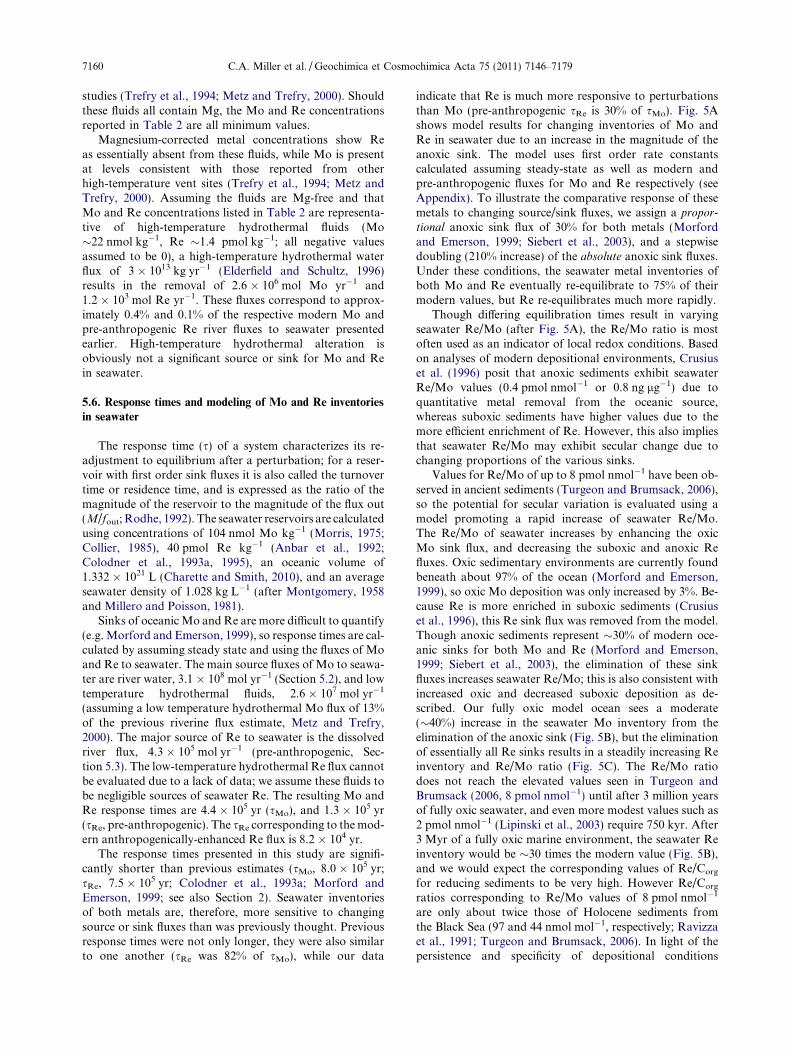
indicate that Re is much more responsive to perturbationsthan Mo (pre-anthropogenic sRe is 30% of sMo). Fig. 5Ashows model results for changing inventories of Mo andRe in seawater due to an increase in the magnitude of theanoxic sink. The model uses first order rate constantscalculated assuming steady-state as well as modern andpre-anthropogenic fluxes for Mo and Re respectively (seeAppendix). To illustrate the comparative response of thesemetals to changing source/sink fluxes, we assign a propor-

tional anoxic sink flux of 30% for both metals (Morfordand Emerson, 1999; Siebert et al., 2003), and a stepwisedoubling (210% increase) of the absolute anoxic sink fluxes.Under these conditions, the seawater metal inventories ofboth Mo and Re eventually re-equilibrate to 75% of theirmodern values, but Re re-equilibrates much more rapidly.

Though differing equilibration times result in varyingseawater Re/Mo (after Fig. 5A), the Re/Mo ratio is mostoften used as an indicator of local redox conditions. Basedon analyses of modern depositional environments, Crusiuset al. (1996) posit that anoxic sediments exhibit seawaterRe/Mo values (0.4 pmol nmol�1 or 0.8 ng lg�1) due toquantitative metal removal from the oceanic source,whereas suboxic sediments have higher values due to themore efficient enrichment of Re. However, this also impliesthat seawater Re/Mo may exhibit secular change due tochanging proportions of the various sinks.

Values for Re/Mo of up to 8 pmol nmol�1 have been ob-served in ancient sediments (Turgeon and Brumsack, 2006),so the potential for secular variation is evaluated using amodel promoting a rapid increase of seawater Re/Mo.The Re/Mo of seawater increases by enhancing the oxicMo sink flux, and decreasing the suboxic and anoxic Refluxes. Oxic sedimentary environments are currently foundbeneath about 97% of the ocean (Morford and Emerson,1999), so oxic Mo deposition was only increased by 3%. Be-cause Re is more enriched in suboxic sediments (Crusiuset al., 1996), this Re sink flux was removed from the model.Though anoxic sediments represent �30% of modern oce-anic sinks for both Mo and Re (Morford and Emerson,1999; Siebert et al., 2003), the elimination of these sinkfluxes increases seawater Re/Mo; this is also consistent withincreased oxic and decreased suboxic deposition as de-scribed. Our fully oxic model ocean sees a moderate(�40%) increase in the seawater Mo inventory from theelimination of the anoxic sink (Fig. 5B), but the eliminationof essentially all Re sinks results in a steadily increasing Reinventory and Re/Mo ratio (Fig. 5C). The Re/Mo ratiodoes not reach the elevated values seen in Turgeon andBrumsack (2006, 8 pmol nmol�1) until after 3 million yearsof fully oxic seawater, and even more modest values such as2 pmol nmol�1 (Lipinski et al., 2003) require 750 kyr. After3 Myr of a fully oxic marine environment, the seawater Reinventory would be �30 times the modern value (Fig. 5B),and we would expect the corresponding values of Re/Corg

for reducing sediments to be very high. However Re/Corg

ratios corresponding to Re/Mo values of 8 pmol nmol�1

are only about twice those of Holocene sediments fromthe Black Sea (97 and 44 nmol mol�1, respectively; Ravizzaet al., 1991; Turgeon and Brumsack, 2006). In light of thepersistence and specificity of depositional conditions

0

1

δ98/9

5 Mo

SW, ‰

2

3

100

120

140

160M

o SW

, % m

od.

0

2

4

6

8

Re/

Mo

SW, x

103

7580859095

100

SW i

nv.,

% m

od.

100

1000

2000

3000 Re SW

, % m

od.

Time, x 105 yr6543210

Time, x 106 yr32.521.510.50

1 5 50 100Oxic Mo deposition, %

10

MoRe

MoRe

D

C

B

A

10%, 2.8 kyr90%, 1,060 kyr75%, 640 kyr

END

START

25%, 7.7 kyr50%,11 kyr

Jurassic τ Mo ≈ 27 kyr

modern τMo ≈ 440 kyr

75%,37 kyr

50%,322 kyr

25%,134 kyr 10%,

49 kyr

90%,61kyr

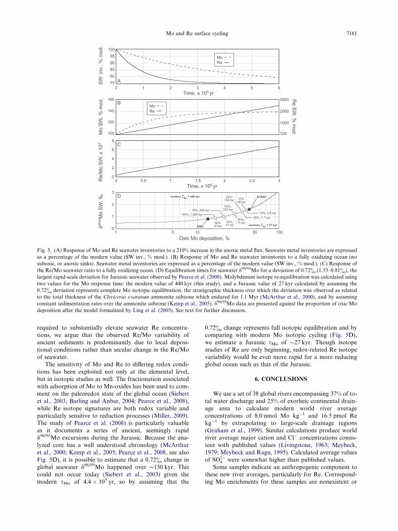
Fig. 5. (A) Response of Mo and Re seawater inventories to a 210% increase in the anoxic metal flux. Seawater metal inventories are expressedas a percentage of the modern value (SW inv., % mod.). (B) Response of Mo and Re seawater inventories to a fully oxidizing ocean (nosuboxic, or anoxic sinks). Seawater metal inventories are expressed as a percentage of the modern value (SW inv., % mod.). (C) Response ofthe Re/Mo seawater ratio to a fully oxidizing ocean. (D) Equilibration times for seawater d98/95Mo for a deviation of 0.72& (1.53–0.81&), thelargest rapid-scale deviation for Jurassic seawater observed by Pearce et al. (2008). Molybdenum isotope re-equilibration was calculated usingtwo values for the Mo response time: the modern value of 440 kyr (this study), and a Jurassic value of 27 kyr calculated by assuming the0.72& deviation represents complete Mo isotopic equilibration, the stratigraphic thickness over which the deviation was observed as relatedto the total thickness of the Cleviceras exaratum ammonite subzone which endured for 1.1 Myr (McArthur et al., 2000), and by assumingconstant sedimentation rates over the ammonite subzone (Kemp et al., 2005). d98/95Mo data are presented against the proportion of oxic Modeposition after the model formalized by Ling et al. (2005). See text for further discussion.

Mo and Re surface cycling 7161

required to substantially elevate seawater Re concentra-tions, we argue that the observed Re/Mo variability ofancient sediments is predominantly due to local deposi-tional conditions rather than secular change in the Re/Moof seawater.

The sensitivity of Mo and Re to differing redox condi-tions has been exploited not only at the elemental level,but in isotopic studies as well. The fractionation associatedwith adsorption of Mo to Mn-oxides has been used to com-ment on the paleoredox state of the global ocean (Siebertet al., 2003; Barling and Anbar, 2004; Pearce et al., 2008),while Re isotope signatures are both redox variable andparticularly sensitive to reduction processes (Miller, 2009).The study of Pearce et al. (2008) is particularly valuableas it documents a series of ancient, seemingly rapidd98/95Mo excursions during the Jurassic. Because the ana-lyzed core has a well understood chronology (McArthuret al., 2000; Kemp et al., 2005; Pearce et al., 2008, see alsoFig. 5D), it is possible to estimate that a 0.72& change inglobal seawater d98/95Mo happened over �150 kyr. Thiscould not occur today (Siebert et al., 2003) given themodern sMo of 4.4 � 105 yr, so by assuming that the

0.72& change represents full isotopic equilibration and bycomparing with modern Mo isotopic cycling (Fig. 5D),we estimate a Jurassic sMo of �27 kyr. Though isotopestudies of Re are only beginning, redox-related Re isotopevariability would be even more rapid for a more reducingglobal ocean such as that of the Jurassic.

6. CONCLUSIONS

We use a set of 38 global rivers encompassing 37% of to-tal water discharge and 25% of exorheic continental drain-age area to calculate modern world river averageconcentrations of 8.0 nmol Mo kg�1 and 16.5 pmol Rekg�1 by extrapolating to large-scale drainage regions(Graham et al., 1999). Similar calculations produce worldriver average major cation and Cl� concentrations consis-tent with published values (Livingstone, 1963; Meybeck,1979; Meybeck and Ragu, 1995). Calculated average valuesof SO2�

4 were somewhat higher than published values.Some samples indicate an anthropogenic component to

these new river averages, particularly for Re. Correspond-ing Mo enrichments for these samples are nonexistent or

Table A.5River time-series samples, sampling dates, and chemical data for Arctic rivers and Mississippi tributaries. Chemical data are listed to the last significant digit. Where the last significant digit is zero,this is indicated by a decimal point or scientific notation. Uncertainties are as listed in Section 3. Data listed as “b.d.” were below the detection limits.

River, date (yr/m/d) H2Oa

(km3 d�1)Mo(nmol kg�1)

Re(pmol kg�1)

Cl(lmol kg�1)

SO4

(lmol kg�1)Na(lmol kg�1)

Mg(lmol kg�1)

Ca(lmol kg�1)

K(lmol kg�1)

Rb(nmol kg�1)

Sr(nmol kg�1)

Ba(nmol kg�1)

Kolyma, 2004/06/11 1.56 1.07 3.6 3.0 � 102 101 46 73 212 22 0.9 460 52Kolyma, 2004/06/15 1.30 1.01 2.7 19 58 42 77 186 17 b.d. 1.0 � 102 43Kolyma, 2004/06/25 1.01 1.28 2.8 21 86 48 82 250. 14 b.d. 110 35Kolyma, 2004/07/15 0.617 1.62 2.9 21 98 58 80. 228 14 b.d. 110 40.Kolyma, 2004/08/10 0.416 1.48 2.6 24 104 63 91 260. 12 b.d. 150 39Kolyma, 2004/08/25 0.536 1.67 2.6 23 116 60. 91 268 12 b.d. 160 37Kolyma, 2004/09/23 0.358 2.3 2.2 31 131 70 121 352 11 b.d. 260 42

Lena, 2004/09/04 0.200 4.3 4.6 1610 320 1600 353 660. 18 5.4 1400 140Lena, 2004/06/05 5.37 2.2 3.0 280. 99 340 233 333 37 60. 600 2.0 � 102

Lena, 2004/06/07 6.69 1.81 3.2 190. 81 250 166 357 20. 7.5 1200 70.Lena, 2004/08/19 3.07 3.9 2.6 21 52 350 141 356 13 2.9 600 59Lena, 2004/08/24 2.69 3.7 2.9 290 116 330 150. 361 12 2.1 500 74Lena, 2004/10/07 2.14 3.4 2.6 290 112 350 168 370. 10. 0.7 500 61Lena, 2004/10/10 2.26 3.0 2.1 157 83 210 175 393 9 0.62 440 63

Lena, 2007/05/26 2.08 1.32 0.72 120. 38 130 73 288 8 2.2 900 62Lena, 2007/05/27 3.15 2.9 1.91 390 108 410 191 390. 27 9 900 93Lena, 2007/05/28 4.94 2.8 2.19 380 103 420 187 385 32 9 800 91Lena, 2007/05/29 6.22 2.2 1.75 450 87 340 158 310. 28 8 600 77Lena, 2007/05/30 7.01 2.0 1.71 320 80. 310 149 294 28 9 600 79Lena, 2007/05/31 7.78 2.0 1.84 310 78 330 149 291 29 9 500 74Lena, 2007/06/02 8.64 1.9 2.12 250 69 270 143 305 30. 9 500 70.Lena, 2007/06/02 8.50 1.9 1.91 250 65 260 142 291 29 9 500 76Lena, 2007/06/04 8.03 1.81 1.96 210 62 230 89 390. 29 8 700 45Lena, 2007/06/05 9.50 1.55 1.58 190 49 190 126 265 24 7 410 70.Lena, 2007/06/06 8.99 1.55 1.69 158 46 180 123 278 24 6 500 70.Lena, 2007/06/08 7.67 1.63 1.51 91 31 130 123 273 24 4.8 320 64Lena, 2007/06/09 7.49 1.50 1.79 90. 31 120 126 285 23 4.5 320 64Lena, 2007/06/10 7.38 0.80 0.78 47 17.6 66 93 255 14 2.7 290 60.Lena, 2007/06/11 7.23 1.45 1.61 79 29 1.0 � 102 139 312 23 4.7 380 69

Ob, 2004/04/05 0.307 5.4 15.9 250 136 250 360. 718 31 10. 1.0 � 103 44Ob, 2004/06/15 2.98 2.6 12.9 117 85 220 129 354 28 5.0 280 63Ob, 2004/06/17 2.98 3.0 13.9 110. 85 220 128 360. 29 4.2 320 66Ob, 2004/07/28 2.25 3.8 1.26 94 62 220 140. 385 32 3.6 380 71Ob, 2004/08/11 1.37 4.1 11.3 116 59 260 159 411 27 3.5 410 72Ob, 2004/10/11 0.771 4.6 11.1 140. 75 320 209 565 21 1.9 600 80.Ob, 2004/10/14 0.829 4.3 10.7 130. 72 320 207 549 20. 3.5 600 79

Ob, 2007/05/29 3.21 0.89 2.09 50. 19 80 49.4 136 13 3.0 80 33Ob, 2007/05/30 3.20 0.56 1.57 97 12.8 68 21.0 174 13 3.5 1.0 � 103 20.Ob, 2007/05/31 3.14 0.38 1.26 60. 9.1 60. 35.5 67.8 12 4.2 30. 23

7162C

.A.

Miller

etal./

Geo

chim

icaet

Co

smo

chim

icaA

cta75

(2011)7146–7179

Ob, 2007/06/01 3.14 0.44 1.57 55 10.3 70 39.0 71.5 14 5.6 33 26Ob, 2007/06/02 3.13 0.60 1.48 67 11.0 55 31.7 75.3 10. 2.7 39 28Ob, 2007/06/03 3.11 0.36 1.41 102 7.7 63 32.9 53.6 13 4.7 15 22Ob, 2007/06/04 3.08 0.35 1.14 54 8.6 62 32.8 57.5 11 3.4 17 25Ob, 2007/06/05 3.03 0.53 2.1 31 13.1 66 40.6 73.2 12 3.3 30. 31Ob, 2007/06/06 3.02 0.44 0.82 79 7.2 55 30.4 53.8 10. 3.8 12 22Ob, 2007/06/07 3.02 0.53 1.30 34 11.4 65 37.2 68.9 12 5.1 31 27Ob, 2007/06/08 3.02 0.43 4.9 48 10.3 50. 32.4 55.6 10. 3.0 16 26Ob, 2007/06/09 3.01 0.47 7.5 53 10.8 58 33.5 58.8 10. 3.0 18 30.Ob, 2007/06/10 3.00 0.74 2.1 30. 14.1 46 36.5 82.8 9 1.9 39 34Ob, 2007/06/11 3.00 1.06 3.1 80. 23 90 52.8 124 14 3.5 90 33Ob, 2007/06/12 3.01 0.22 0.78 20. 3.2 31 17.1 40.7 5.2 1.1 b.d. 21Ob, 2007/06/13 3.01 0.61 1.35 51 12.7 70 38.2 80.3 11 3.5 42 26Ob, 2007/06/14 3.01 0.47 1.9 63 10.8 70 37.8 65.3 10. 4.2 30. 31Ob, 2007/06/15 3.08 0.49 0.96 36 11.4 80 39.6 84.3 13 b.d. 30. 16Ob, 2007/06/16 3.10 0.67 1.60 40. 13.9 70 41.0 92.3 10. 3.2 45 29Ob, 2007/06/17 3.11 0.68 1.43 25 6.2 40. 24.1 57.9 5.8 1.3 9 23

Yenisei, 2004/03/19 0.638 6.7 9.9 3.0 � 102 144 380 214 664 20. 1.9 1400 82Yenisei, 2004/06/14 8.51 1.53 3.0 44 28 6.0 61.5 164 0.56 b.d. 150 28Yenisei, 2004/06/16 8.16 0.74 4.1 61 27 90 60.8 164 8 b.d. 140 27Yenisei, 2004/06/18 7.83 0.88 4.6 63 31 1.0 � 102 75 168 9 1.6 180 34Yenisei, 2004/08/25 1.57 6.0 10.3 280 105 360 195 506 16 2.6 1.0 � 103 65Yenisei, 2004/10/01 1.72 3.9 7.1 180 87 3.0 � 102 163 454 12 0.7 800 54Yenisei, 2004/10/02 1.67 4.1 7.1 250 87 3.0 � 102 162 442 11 0.32 800 50.

Mackenzie, 2004/03/24 0.327 9.3 16.8 380 410 5.0 � 102 374 847 24 4.4 1400 260Mackenzie, 2004/06/17 1.58 9.0 14.9 143 310 240 307 817 20. 5.4 1200 250Mackenzie, 2004/06/22 1.50 2.8 15.5 130. 310 220 308 766 22 9 1.0 � 103 3.0 � 102

Mackenzie, 2004/07/13 1.08 10.4 16.2 181 360 290 336 868 20. 4.7 1100 240Mackenzie, 2004/08/04 0.07 11.5 20. 210 4.0 � 102 330 369 903 22 5.6 1400 250Mackenzie, 2004/08/25 0.754 13.0 15.8 240 410 370 412 980 28 19 1600 380Mackenzie, 2004/08/09 0.758 13.2 15.7 260 430 4.0 � 102 402 950 26 11 1600 310

Yukon, 2004/04/07 0.1138 13.6 12.0 79 280 160 332 818 33 13 700 140Yukon, 2004/05/26 1.282 5.1 8.1 43 152 80 187 593 25 8 410 160Yukon, 2004/06/15 1.563 7.6 10.8 42 2.0 � 102 70 212 717 27 10. 320 2.0 � 102

Yukon, 2004/06/29 1.258 19 12.3 69 250 1.0 � 102 258 812 29 12 500 220Yukon, 2004/07/19 0.8685 13.9 15.6 74 310 140 322 800 54 35 700 260Yukon, 2004/08/18 0.8172 14.6 17.5 66 4.0 � 102 160 391 828 63 55 900 410Yukon, 2004/09/22 0.4942 14.1 17.8 85 390 160 381 970 42 19 900 250

Arkansas, 2004/02/12 0.112 6.6 19 1110 280 – – – – – – –Arkansas, 2004/04/15 0.122 9.3 27 1390 370 – – – – – – –Arkansas, 2004/07/17 0.205 9.3 22 1350 320 – – – – – – –Arkansas, 2004/11/13 0.113 12.4 17.7 1520 310 – – – – – – –

(continued on next page)

Mo

and

Re

surface

cycling

7163

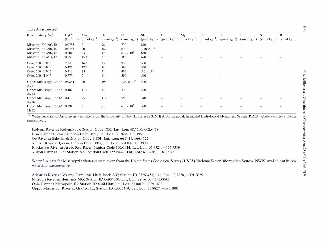
Table A.5 (continued)

River, date (yr/m/d) H2Oa

(km3 d�1)Mo(nmol kg�1)

Re(pmol kg�1)

Cl(lmol kg�1)

SO4

(lmol kg�1)Na(lmol kg�1)

Mg(lmol kg�1)

Ca(lmol kg�1)

K(lmol kg�1)

Rb(nmol kg�1)

Sr(nmol kg�1)

Ba(nmol kg�1)

Missouri, 2004/02/10 0.0785 21 96 770 810 – – – – – – –Missouri, 2004/04/14 0.0785 30. 164 610 1.10 � 103 – – – – – – –Missouri, 2004/07/12 0.204 33 123 6.0 � 102 880 – – – – – – –Missouri, 2004/11/12 0.153 15.6 57 360 420 – – – – – – –

Ohio, 2004/02/12 2.14 16.0 25 710 540 – – – – – – –Ohio, 2004/04/14 0.484 17.0 34 590 520 – – – – – – –Ohio, 2004/07/17 0.519 35 51 480 5.0 � 102 – – – – – – –Ohio, 2004/11/13 0.776 21 43 500 560 – – – – – – –

Upper Mississippi, 2004/02/11

0.0864 26 106 1.20 � 103 440 – – – – – – –

Upper Mississippi, 2004/04/14

0.409 11.0 45 570 270 – – – – – – –

Upper Mississippi, 2004/07/16

0.416 25 112 550 340 – – – – – – –

Upper Mississippi, 2004/11/12

0.294 21 91 6.0 � 102 320 – – – – – – –

a Water flux data for Arctic rivers were taken from the University of New Hampshire’s (UNH) Arctic Regional, Integrated Hydrological Monitoring System (RIMS) website available at http://rims.unh.edu/.

Kolyma River at Kolymskoye; Station Code 1802; Lat, Lon: 68.7500, 002.6458Lena River at Kusur; Station Code 3821; Lat, Lon: 66.7664, 123.3967Ob River at Salekhard; Station Code 11801; Lat, Lon: 66.5414, 066.4722Yenisei River at Igarka; Station Code 9803; Lat, Lon: 67.4344, 086.3908Mackenzie River at Arctic Red River; Station Code 10LC014; Lat, Lon: 67.4521, �133.7389Yukon River at Pilot Station AK; Station Code 15565447; Lat, Lon: 61.9486, �162.9077

Water flux data for Mississippi tributaries were taken from the United States Geological Survey (USGS) National Water Information System (NWIS) available at http://waterdata.usgs.gov/nwis/.

Arkansas River at Murray Dam near Little Rock AK; Station ID 07263450; Lat, Lon: 33.9878, �091.3625Missouri River at Hermann MO; Station ID 06934500; Lat, Lon: 38.5610, �092.0092Ohio River at Metropolis IL; Station ID 03611500; Lat, Lon: 37.0010, �089.1638Upper Mississippi River at Grafton IL; Station ID 05587450; Lat, Lon: 38.8827, �090.1882

7164C

.A.

Miller

etal./

Geo

chim

icaet

Co

smo

chim

icaA

cta75

(2011)7146–7179

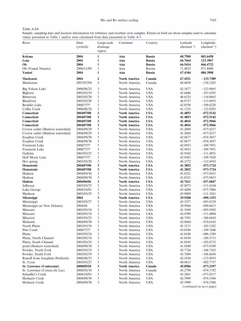
Table A.6ASample, sampling date and location information for tributary and exorheic river samples. Entries in bold are those samples used to calculatevalues presented in Table 1 and/or were calculated from data presented in Table A.5.

River Date(yr/m/d)

Large-scaledrainageregion

Continent Country Latitude(decimal �)

Longitude(decimal �)

Kolyma 2004 1 Asia Russia 68.7500 002.6458

Lena 2004 1 Asia Russia 66.7664 123.3967

Ob 2004 1 Asia Russia 66.5414 066.4722

Ob (Yamal Nemetz) 2006/11/09 1 Asia Russia 71.4833 071.8000Yenisei 2004 1 Asia Russia 67.4344 086.3908

Mackenzie 2004 2 North America Canada 67.4521 �133.7389

Mackenzie 2007/07/04 2 North America Canada 68.4659 �134.1283

Big Vulcan Lake 2000/08/23 3 North America USA 42.1877 �123.9845Bighorn 2005/05/19 3 North America USA 45.6446 �107.6585Bitterroot 2005/05/20 3 North America USA 46.6323 �114.0663Blackfoot 2005/05/20 3 North America USA 46.8737 �113.8855Boulder Lake 2000/??/?? 3 North America USA 42.8558 �109.6228Coffee Creek 2000/08/26 3 North America USA 41.1235 �122.8203Connecticut 2004/07/08 3 North America USA 41.4853 �072.5142

Connecticut 2004/07/08 3 North America USA 41.4853 �072.5142

Connecticut 2004/07/08 3 North America USA 41.4816 �072.5066

Connecticut 2004/07/08 3 North America USA 41.4816 �072.5066

Croton outlet (Hudson watershed) 2004/09/29 3 North America USA 41.2069 �073.8217Croton outlet (Hudson watershed) 2004/09/29 3 North America USA 41.2069 �073.8217Esophus Creek 2004/09/30 3 North America USA 42.0677 �074.3057Esophus Creek 2004/09/30 3 North America USA 42.0677 �074.3057Freemont Lake 2000/??/?? 3 North America USA 42.9453 �109.7951Freemont Lake 2000/??/?? 3 North America USA 42.9453 �109.7951Gallatin 2005/05/25 3 North America USA 45.9342 �111.4931Half Moon Lake 2000/??/?? 3 North America USA 42.9365 �109.7620Hot spring 2005/05/20 3 North America USA 46.1372 �112.8918Housatonic 2004/07/08 3 North America USA 41.3852 �073.1724

Housatonic 2004/07/08 3 North America USA 41.3852 �073.1724

Hudson 2004/09/30 3 North America USA 41.8321 �073.9415Hudson 2004/09/30 3 North America USA 41.8321 �073.9415Hudson 2006/06/06 3 North America USA 42.7611 �037.6847

Jefferson 2005/05/25 3 North America USA 45.8973 �111.6104Lake George 2004/10/01 3 North America USA 43.4200 �073.7086Madison 2005/05/25 3 North America USA 45.9009 �111.5261Mississippi 2004 3 North America USA 29.9208 �090.1353

Mississippi 2005/05/27 3 North America USA 45.3257 �093.8239Mississippi (at New Orleans) 2004/04 3 North America USA 29.9566 �090.0615Missouri 2005/05/18 3 North America USA 41.3569 �095.9502Missouri 2005/05/19 3 North America USA 45.9399 �111.4904Missouri 2005/05/25 3 North America USA 46.7591 �100.8410Mohawk 2004/09/30 3 North America USA 42.8484 �074.0143North Platte 2005/05/18 3 North America USA 41.3171 �102.1262Pine Creek 2000/??/?? 3 North America USA 43.0349 �109.7648Platte 2005/05/18 3 North America USA 41.0148 �096.1580Platte, North Channel 2005/05/18 3 North America USA 41.0194 �100.3715Platte, South Channel 2005/05/18 3 North America USA 41.0545 �102.0732pond (Hudson watershed) 2004/09/30 3 North America USA 41.9240 �073.9109Powder, North Fork 2005/05/19 3 North America USA 43.7726 �106.7103Powder, South Fork 2005/05/19 3 North America USA 43.7084 �106.6036Runoff from Josephine Peridotite 2000/08/23 3 North America USA 42.1836 �123.9933St. Croix 2005/05/27 3 North America USA 44.9613 �092.7737St. Lawrence (Contrecœur) 2008/05/18 3 North America Canada 45.8586 �073.2397

St. Lawrence (Coteau du Lac) 2008/05/18 3 North America Canada 45.2798 �074.1782Schaeffer’s Creek 2004/10/01 3 North America USA 43.2861 �073.8217Shoharie Creek 2004/09/30 3 North America USA 42.5999 �074.3360Shoharie Creek 2004/09/30 3 North America USA 42.5999 �074.3360

(continued on next page)

Mo and Re surface cycling 7165

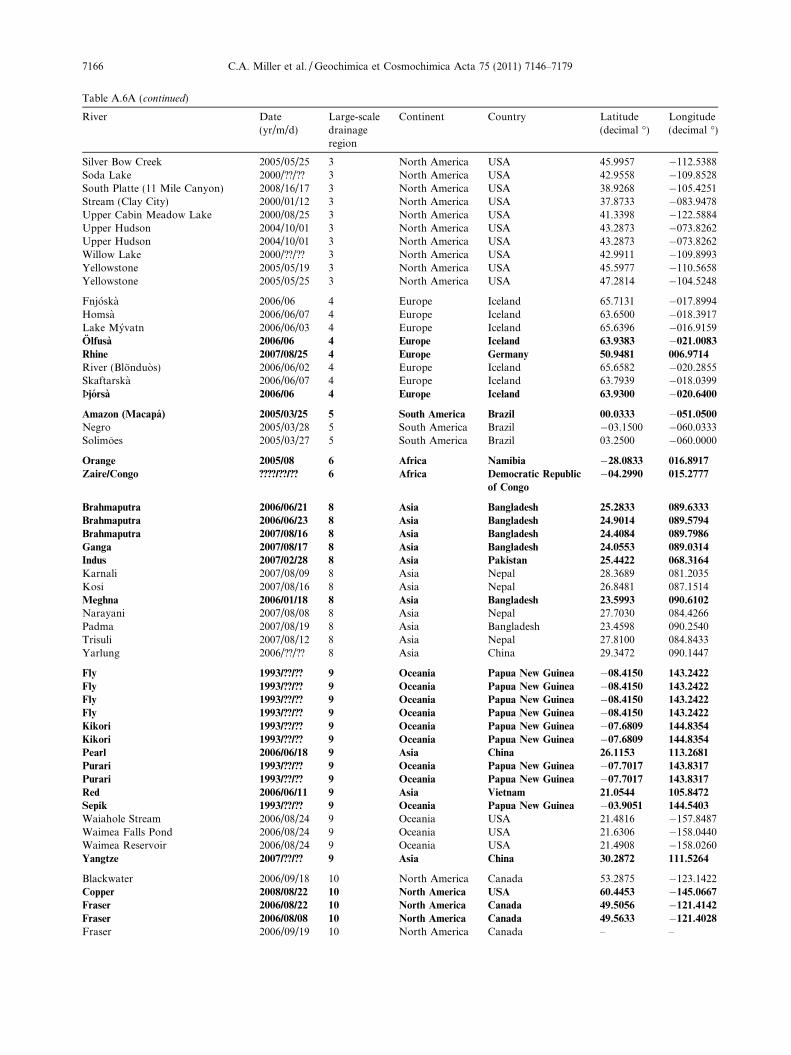
Table A.6A (continued)

River Date(yr/m/d)

Large-scaledrainageregion

Continent Country Latitude(decimal �)

Longitude(decimal �)

Silver Bow Creek 2005/05/25 3 North America USA 45.9957 �112.5388Soda Lake 2000/??/?? 3 North America USA 42.9558 �109.8528South Platte (11 Mile Canyon) 2008/16/17 3 North America USA 38.9268 �105.4251Stream (Clay City) 2000/01/12 3 North America USA 37.8733 �083.9478Upper Cabin Meadow Lake 2000/08/25 3 North America USA 41.3398 �122.5884Upper Hudson 2004/10/01 3 North America USA 43.2873 �073.8262Upper Hudson 2004/10/01 3 North America USA 43.2873 �073.8262Willow Lake 2000/??/?? 3 North America USA 42.9911 �109.8993Yellowstone 2005/05/19 3 North America USA 45.5977 �110.5658Yellowstone 2005/05/25 3 North America USA 47.2814 �104.5248

Fnjoska 2006/06 4 Europe Iceland 65.7131 �017.8994Homsa 2006/06/07 4 Europe Iceland 63.6500 �018.3917Lake Myvatn 2006/06/03 4 Europe Iceland 65.6396 �016.9159Olfusa 2006/06 4 Europe Iceland 63.9383 �021.0083

Rhine 2007/08/25 4 Europe Germany 50.9481 006.9714

River (Blonduos) 2006/06/02 4 Europe Iceland 65.6582 �020.2855Skaftarska 2006/06/07 4 Europe Iceland 63.7939 �018.0399Þjorsa 2006/06 4 Europe Iceland 63.9300 �020.6400

Amazon (Macapa) 2005/03/25 5 South America Brazil 00.0333 �051.0500

Negro 2005/03/28 5 South America Brazil �03.1500 �060.0333Solimoes 2005/03/27 5 South America Brazil 03.2500 �060.0000

Orange 2005/08 6 Africa Namibia �28.0833 016.8917

Zaire/Congo ????/??/?? 6 Africa Democratic Republic

of Congo

�04.2990 015.2777

Brahmaputra 2006/06/21 8 Asia Bangladesh 25.2833 089.6333

Brahmaputra 2006/06/23 8 Asia Bangladesh 24.9014 089.5794

Brahmaputra 2007/08/16 8 Asia Bangladesh 24.4084 089.7986

Ganga 2007/08/17 8 Asia Bangladesh 24.0553 089.0314

Indus 2007/02/28 8 Asia Pakistan 25.4422 068.3164

Karnali 2007/08/09 8 Asia Nepal 28.3689 081.2035Kosi 2007/08/16 8 Asia Nepal 26.8481 087.1514Meghna 2006/01/18 8 Asia Bangladesh 23.5993 090.6102

Narayani 2007/08/08 8 Asia Nepal 27.7030 084.4266Padma 2007/08/19 8 Asia Bangladesh 23.4598 090.2540Trisuli 2007/08/12 8 Asia Nepal 27.8100 084.8433Yarlung 2006/??/?? 8 Asia China 29.3472 090.1447

Fly 1993/??/?? 9 Oceania Papua New Guinea �08.4150 143.2422

Fly 1993/??/?? 9 Oceania Papua New Guinea �08.4150 143.2422

Fly 1993/??/?? 9 Oceania Papua New Guinea �08.4150 143.2422

Fly 1993/??/?? 9 Oceania Papua New Guinea �08.4150 143.2422

Kikori 1993/??/?? 9 Oceania Papua New Guinea �07.6809 144.8354

Kikori 1993/??/?? 9 Oceania Papua New Guinea �07.6809 144.8354

Pearl 2006/06/18 9 Asia China 26.1153 113.2681

Purari 1993/??/?? 9 Oceania Papua New Guinea �07.7017 143.8317

Purari 1993/??/?? 9 Oceania Papua New Guinea �07.7017 143.8317

Red 2006/06/11 9 Asia Vietnam 21.0544 105.8472

Sepik 1993/??/?? 9 Oceania Papua New Guinea �03.9051 144.5403

Waiahole Stream 2006/08/24 9 Oceania USA 21.4816 �157.8487Waimea Falls Pond 2006/08/24 9 Oceania USA 21.6306 �158.0440Waimea Reservoir 2006/08/24 9 Oceania USA 21.4908 �158.0260Yangtze 2007/??/?? 9 Asia China 30.2872 111.5264

Blackwater 2006/09/18 10 North America Canada 53.2875 �123.1422Copper 2008/08/22 10 North America USA 60.4453 �145.0667

Fraser 2006/08/22 10 North America Canada 49.5056 �121.4142

Fraser 2006/08/08 10 North America Canada 49.5633 �121.4028

Fraser 2006/09/19 10 North America Canada – –

7166 C.A. Miller et al. / Geochimica et Cosmochimica Acta 75 (2011) 7146–7179

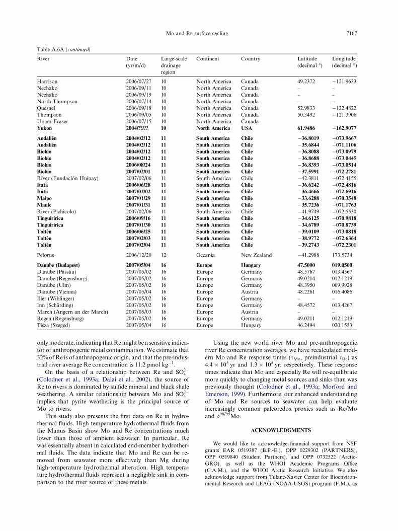
Table A.6A (continued)

River Date(yr/m/d)

Large-scaledrainageregion

Continent Country Latitude(decimal �)

Longitude(decimal �)

Harrison 2006/07/27 10 North America Canada 49.2372 �121.9633Nechako 2006/09/11 10 North America Canada – –Nechako 2006/09/19 10 North America Canada – –North Thompson 2006/07/14 10 North America Canada – –Quesnel 2006/09/18 10 North America Canada 52.9833 �122.4822Thompson 2006/09/05 10 North America Canada 50.3492 �121.3906Upper Fraser 2006/07/15 10 North America CanadaYukon 2004/??/?? 10 North America USA 61.9486 �162.9077

Andalien 2004/02/12 11 South America Chile �36.8019 �073.9667

Andalien 2004/02/12 11 South America Chile �35.6844 �071.1106

Biobıo 2004/02/12 11 South America Chile �36.8088 �073.0979

Biobıo 2004/02/12 11 South America Chile �36.8688 �073.0445

Biobıo 2006/08/24 11 South America Chile �36.8393 �073.0514

Biobıo 2007/02/01 11 South America Chile �37.5991 �072.2781

River (Fundacion Huinay) 2007/02/06 11 South America Chile �42.3811 �072.4155Itata 2006/06/28 11 South America Chile �36.6242 �072.4816

Itata 2007/02/02 11 South America Chile �36.4666 �072.6916

Maipo 2007/01/29 11 South America Chile �33.6288 �070.3548

Maule 2007/01/31 11 South America Chile �35.7236 �071.1763

River (Pichicolo) 2007/02/06 11 South America Chile �41.9749 �072.5530Tinguiririca 2006/09/16 11 South America Chile �34.6125 �070.9818

Tinguiririca 2007/01/30 11 South America Chile �34.6789 �070.8739

Tolten 2006/06/25 11 South America Chile �39.0109 �073.0818

Tolten 2007/02/03 11 South America Chile �38.9772 �072.6364

Tolten 2007/02/04 11 South America Chile �39.2743 �072.2301

Pelorus 2006/12/20 12 Oceania New Zealand �41.2988 173.5734

Danube (Budapest) 2007/05/04 16 Europe Hungary 47.5000 019.0500

Danube (Passau) 2007/05/02 16 Europe Germany 48.5767 013.4567Danube (Regensburg) 2007/05/02 16 Europe Germany 49.0214 012.1219Danube (Ulm) 2007/05/02 16 Europe Germany 48.3950 009.9928Danube (Vienna) 2007/05/04 16 Europe Austria 48.2261 016.4086Iller (Wiblinger) 2007/05/02 16 Europe Germany – –Inn (Scharding) 2007/05/02 16 Europe Germany 48.4572 013.4267March (Angern an der March) 2007/05/03 16 Europe Austria – –Regen (Regensburg) 2007/05/02 16 Europe Germany 49.0211 012.1219Tisza (Szeged) 2007/05/04 16 Europe Hungary 46.2494 020.1533

Mo and Re surface cycling 7167

only moderate, indicating that Re might be a sensitive indica-tor of anthropogenic metal contamination. We estimate that32% of Re is of anthropogenic origin, and that the pre-indus-trial river average Re concentration is 11.2 pmol kg�1.

On the basis of a relationship between Re and SO2�4

(Colodner et al., 1993a; Dalai et al., 2002), the source ofRe to rivers is dominated by sulfide mineral and black shaleweathering. A similar relationship between Mo and SO2�

4

implies that pyrite weathering is the principal source ofMo to rivers.

This study also presents the first data on Re in hydro-thermal fluids. High temperature hydrothermal fluids fromthe Manus Basin show Mo and Re concentrations muchlower than those of ambient seawater. In particular, Rewas essentially absent in calculated end-member hydrother-mal fluids. The data indicate that Mo and Re can be re-moved from seawater more effectively than Mg duringhigh-temperature hydrothermal alteration. High tempera-ture hydrothermal fluids represent a negligible sink in com-parison to the river source of these metals.

Using the new world river Mo and pre-anthropogenicriver Re concentration averages, we have recalculated mod-ern Mo and Re response times (sMo, preindustrial sRe) as4.4 � 105 yr and 1.3 � 105 yr, respectively. These responsetimes indicate that Mo and especially Re will re-equilibratemore quickly to changing metal sources and sinks than waspreviously thought (Colodner et al., 1993a; Morford andEmerson, 1999). Furthermore, our enhanced understandingof Mo and Re sources to seawater can help evaluateincreasingly common paleoredox proxies such as Re/Moand d98/95Mo.

ACKNOWLEDGMENTS

We would like to acknowledge financial support from NSFgrants EAR 0519387 (B.P.-E.), OPP 0229302 (PARTNERS),OPP 0519840 (Student Partners), and OPP 0732522 (Arctic-GRO), as well as the WHOI Academic Programs Office(C.A.M.), and the WHOI Arctic Research Initiative. We alsoacknowledge support from Tulane-Xavier Center for Bioenviron-mental Research and LEAG (NOAA-USGS) program (F.M.), as

Table A.6BSample ID and chemical data for tributary and exorheic river samples. Entries in bold are those samples used to calculate values presented in Table 1 and/or were calculated from data presented inTable A.5. Data listed as ”b.d.” were below the detection limits.

River Mo(nmol kg�1)

Re(pmol kg�1)

Cl(lmol kg�1)

SO4

(lmol kg�1)Na(lmol kg�1)

Mg(lmol kg�1)

Ca(lmol kg�1)

K(lmol kg�1)

Rb(nmol kg�1)

Sr(nmol kg�1)

Ba(nmol kg�1)

Kolyma 1.47 2.9 92 100. 55 87 250 15 b.d. 230 42

Lena 3.0 2.9 260 96 370 178 380 16 5.3 800 78

Ob 3.9 12.5 135 83 3.0 � 102 185 460 28 4.7 500 66

Ob (Yamal Nemetz) 2.8 7.6 1770 630 230 185 430 23 3.6 430 84Yenisei 3.5 6.5 168 73 2.0 � 102 131 360 10 1.0 600 49

Mackenzie 10.1 16.2 240 380 350 359 870 23 7 1300 270

Mackenzie 11.1 14.1 440 440 70 414 1.0 � 103 3.5 0.7 2100 280

Big Vulcan Lake b.d. 0.13 25 3.1 33 333 10. 0.36 b.d. b.d. 17Bighorn 28 1.9 � 102 430 3700 4700 1350 1400 140 31 8000 240Bitterroot 3.8 1.23 14.4 18.5 90 41.6 140 23 3.5 70 60.Blackfoot 2.9 2.9 14.6 40 7 285 580 1.7 0.28 170 620Boulder Lake 0.67 4.0 6.6 13.2 28 14.9 56 10 3.1 b.d. 28Coffee Creek 3.3 3.4 190 16.5 180 444 540 4.0 b.d. 32 20Connecticut 7.8 14.9 – – – – – – – – –Connecticut 7.7 14.8 – – – – – – – – –Connecticut 7.9 13.9 – – – – – – – – –Connecticut 7.9 13.9 – – – – – – – – –Croton outlet (Hudsonwatershed)

4.8 5.7 1520 108 1.0 � 103 293 6.0 � 102 52 9 120 120

Croton outlet (Hudsonwatershed)

4.9 5.7 1530 108 1100 296 6.0 � 102 53 10. 110 131

Esophus Creek 0.12 3.7 66 46 90 35.7 120 8 b.d. b.d. 48Esophus Creek 0.14 3.7 66 47 90 36.3 120 8 b.d. b.d. 47Freemont Lake 1.17 6.6 8.5 15.2 25 11.4 51 10. 2.9 b.d. 28Freemont Lake 1.29 6.7 9.4 15.1 25 11.9 52 9 1.9 b.d. 26Gallatin 7.6 11.3 51 159 230 300 730 44 10. 680 181Half Moon Lake 0.65 4.1 7.2 13.3 25 15.1 52 8 0.8 b.d. 27hot spring 33 8.2 13.3 79 90 174 610 25 13 170 83Housatonic 5.4 6.7 – – – – – – – – –Housatonic 5.6 6.6 – – – – – – – – –Hudson 5.7 7.7 520 126 450 173 640 38 3.8 350 88Hudson 4.2 7.7 520 127 460 173 660 38 3.3 340 99Hudson 3.2 7.2 660 124 – – – – – – –Jefferson 23 17.8 91 268 340 291 640 55 11 500 170Lake George 1.34 5.2 470 80. 410 102 350 13 b.d. 38 36Madison 52 10.2 510 126 1500 197 5.0 � 102 1.0 � 102 190 3.0 � 102 107Mississippi 21 57 640 510 – – – – – – –Mississippi 8.2 13.5 250 96 2.0 � 102 521 1.0 � 103 36 9 180 230Mississippi (New Orleans) 13.9 29 760 460 660 478 1.0 � 103 47 2.3 600 260Missouri 39 3.3 � 102 490 1810 2100 1140 1600 140 20. 3600 310

7168C

.A.

Miller

etal./

Geo

chim

icaet

Co

smo

chim

icaA

cta75

(2011)7146–7179

Missouri 14.0 14.9 110. 220 4.0 � 102 364 870 60 26 800 2.0 � 102

Missouri 32 93 320 1840 2900 860 1200 1.0 � 102 18 2900 270Mohawk 4.5 7.8 5.0 � 102 153 480 207 860 31 b.d. 800 104North Platte 27 3.0 � 102 370 1090 2400 483 930 230 61 3.0 � 103 6.0 � 102

Pine Creek 1.44 3.6 5.6 17.5 24 11.7 75 11 2.7 b.d. 33Platte 36 220 280 – 900 633 1600 247 21 2400 730Platte, North Channel 30. 44 77 147 610 276 1400 239 49 1900 1.0 � 103

Platte, South Channel 34 1240 3.0 � 103 9.0 � 103 9000 2460 3900 483 62 14000 190Pond (Hudson watershed) 1.47 6.2 710 111 6.0 � 102 134 870 33 b.d. 5.0 � 102 77Powder, North Fork 8.8 87 102 1780 1800 960 1600 55 7.9 4200 220Powder, South Fork 7.6 16.8 250 770 650 472 1.0 � 103 39 5.0 2500 100Runoff from Josephine Peridotite b.d. 0.29 34 4.8 44 424 10. 2.6 b.d. b.d. 24St. Croix 3.5 8.6 157 44 120 306 550 24 4.5 26 81St. Lawrence (Contrecœur) 12.1 24 580 230 520 292 810 35 10. 1200 109

St. Lawrence (Coteau du Lac) 12.3 17.8 610 240 520 300. 850 36 9 1200 106Schaeffer’s Creek 2.57 4.7 181 65 160 370. 520 12 b.d. b.d. b.d.Shoharie Creek 0.87 4.3 180. 57 190 62.3 280 21 b.d. 12 57Shoharie Creek 0.94 4.3 181 57 190 62.4 290 20 b.d. 6.7 56Silver Bow Creek 82 40. 250 – 390 262 710 61 7 1100 160Soda Lake 4.9 42 6300 – 3100 6150 2100 3200 130 1300 86South Platte (11 Mile Canyon) 19 37 1220 580 1500 611 1.0 � 103 51 7 2600 190Stream (Clay City) 11.7 157 660 3500 2.0 � 102 395 1.0 � 103 110 29 500 93Upper Cabin Meadow Lake b.d. 0.29 2.1 0.73 4.8 342 9.4 0.9 b.d. b.d. 160Upper Hudson 1.24 3.9 3.0 � 102 48 240 54.7 210 8 2.3 23 37Upper Hudson 1.02 3.9 3.0 � 102 48 240 54.3 210 8 2.2 18 45Willow Lake 0.43 9.4 20. 23 47 21.3 73 13 1.6 15 42Yellowstone 7.0 4.1 75 97 310 136 280 52 64 220 80Yellowstone 11.3 29 94 560 700 339 650 46 12 900 150

Fnjoska 0.42 0.92 33 3.8 65 20.4 45 2.2 b.d. b.d. 12.6Homsa 2.3 1.83 78 28 220 72.6 110 12 1.2 b.d. 20Lake Myvatn 10.6 11.2 – – 1200 203 340 60 34 b.d. 16Olfusa 1.04 1.74 153 24 3.0 � 102 56.5 1.0 � 102 12 2.0 b.d. 3300

Rhine 10.8 57 1210 390 800 356 1500 80 24 2600 190

River (Blonduos) 1.32 1.39 93 18 15 89 110 10 b.d. b.d. 18Skaftarska 1.76 3.6 87 79 270 78 160 9 b.d. b.d. b.d.Þjorsa 4.1 4.1 86 61 320 63.1 1.0 � 102 11 b.d. b.d. 13.4

Amazon (Macapa) 0.89 1.83 – 92 1.0 � 102 67.8 160 30 40. 150 240

Negro 0.15 b.d. – – 17 3.1 5.9 4.9 9 b.d. 336Solimoes 0.65 3.0 – 23 130 91 310 29 41 390 330

Orange 24 37 2800 1210 3600 1090 1.0 � 103 60 1.9 2.0 � 103 330

Zaire/Congo 0.45 3.0 36 17.9 90 62.1 523 39 31 17 79

Brahmaputra 13.2 5.4 44 190 220 253 7.0 � 102 60 28 600 99

Brahmaputra 11.8 4.8 44 174 210 263 7.0 � 102 59 26 600 95

Brahmaputra 8.4 3.0 40 102 93 134 450 57 27 240 73

(continued on next page)

Mo

and

Re

surface

cycling

7169

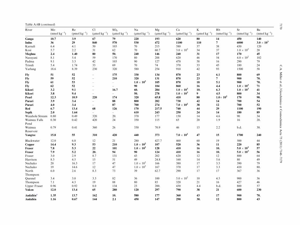
Table A.6B (continued)

River Mo(nmol kg�1)

Re(pmol kg�1)

Cl(lmol kg�1)

SO4

(lmol kg�1)Na(lmol kg�1)

Mg(lmol kg�1)

Ca(lmol kg�1)

K(lmol kg�1)

Rb(nmol kg�1)

Sr(nmol kg�1)

Ba(nmol kg�1)

Ganga 10.7 3.9 67 79 220 193 620 80 14 450 140

Indus 36 29 840 570 530 472 1100 110 7 6000 3.0 � 103

Karnali 6.4 4.1 50 103 70 215 580 37 38 430 120Kosi 5.7 2.2 31 62 70 60.7 3.0 � 102 34 37 1.0 � 102 20Meghna 2.4 1.40 80 50. 240 146 240 31 17 170 45

Narayani 8.1 5.4 59 170 80 288 620 46 54 4.0 � 102 102Padma 9.1 3.3 42 103 90 127 470 58 16 290 79Trisuli 5.4 1.74 33 69 70 74 370 33 45 180 24Yarlung 18.6 8.39 230 320 580 254 910 42 93 1500 58

Fly 51 52 – 175 330 134 870 23 6.1 800 69

Fly 59 52 – 210 320 131 870 23 7 900 70.

Fly 61 53 – – 1.0 � 102 105 870 18 5.1 900 70.

Fly 62 52 – – 90 104 860 16 4.4 1.0 � 103 71

Kikori 3.2 9.1 – 16.7 60. 284 1.0 � 103 10. 6.3 1.0 � 103 41

Kikori 3.8 9.4 – – 50. 278 1.0 � 103 9 4.5 800 34

Pearl 12.3 10.9 220 174 320 65.8 410 80 1.0� 102 170 90.

Purari 3.9 3.4 – 88 800 282 730 42 14 700 54

Purari 4.0 3.4 – 87 700 274 7.0 � 102 38 12 700 52

Red 6.7 13.4 68 126 170 217.5 740 44 29 1100 190

Sepik 2.0 1.64 – – 610 243 250 24 14 180 89

Waiahole Stream 0.80 0.49 320 20. 370 177 150 14 4.6 90 34Waimea FallsPond

0.30 0.42 420 24 350 115 65 20 1.9 16 20.

WaimeaReservoir

0.79 0.41 360 26 330 70.9 46 15 2.2 b.d. 30.

Yangtze 15.8 55 310 420 440 373 7.0 � 102 47 15 1700 240

Blackwater 12.0 6.0 12 21 280 427.7 460 60 19 500 44Copper 14.4 9.3 53 210 1.0 � 102 107 520 36 11 220 85

Fraser 7.8 5.3 22 101 1.0 � 102 128 410 16 10. 5.0 � 103 57

Fraser 7.9 5.2 20. 94 90 124 410 16 10. 5.0 � 103 56

Fraser 3.0 2.9 8.7 131 43 202 620 12 12 800 64Harrison 8.3 4.5 15 51 49 24.8 160 14 5.6 80 49Nechako 20 16.3 17 47 1.0 � 102 166 380 17 3.5 390 79Nechako 19 14.6 12 47 1.0 � 102 167 370 17 3.3 410 80.NorthThompson

6.0 2.6 8.3 73 39 62.7 290 17 17 367 36

Quesnel 3.4 3.0 3.3 82 36 100 5.0 � 102 10 4.5 900 36Thompson 7.1 4.3 19 88 80 85 320 21 16 427 46Upper Fraser 0.96 0.92 8.0 134 23 200. 430 4.4 b.d. 800 57Yukon 12.0 13.4 65 280 120 297 790 38 21 600 230

Andaliena 1.35 13.7 162 10. 580 177 360 43 17 900 70.

Andalien 1.16 0.67 144 2.1 450 147 290 30. 12 800 43

7170C

.A.

Miller

etal./

Geo

chim

icaet

Co

smo

chim

icaA

cta75

(2011)7146–7179

Biobıoa 2.1 5.7 88 50. 250 113 220 27 22 320 19

Biobıo 2.0 6.7 89 51 240 99 180 25 23 270 18

Biobıo 2.2 3.5 67 28 180 93 140 22 17 230 16

Biobıo 2.9 3.8 136 59 210 93 210 28 32 26 20

river (Fundacion Huinay) 5.0 3.8 28 24 47 45 250 160 20. 1700 4.4Itataa 2.9 1.60 53 29 190 94 120 22 24 280 20.

Itata 6.5 0.69 330 3.5 900 472 430 46 3.0 1500 126

Maipoa 33 53 2500 3300 2900 387 3700 70 70 1.0 � 104 86

Maulea 19 7.4 190 174 360 129 280 33 46 440 22

River at Pichicolo 68 2.78 2800 610 3800 34 320 21 40 210 8.7Tinguiriricaa 12.6 17.0 161 370 330 110. 540 26 39 800 25

Tinguiririca 16.3 24 117 540 240 114 470 31 43 600 21

Tolten 3.3 1.55 40. 15.6 140 55.6 1.0 � 103 19 17 140 14

Toltena 5.5 2.2 49 28 2.0 � 102 75 130 25 23 160 24

Tolten 5.1 1.88 35 19 160 66.4 120 22 22 180 12.5

Pelorus 1.9 0.59 85 21 140 105 160 8 b.d. 70 20Danube (Budapest) 10.8 74 1830 1030 2.0 � 103 1.20 � 103 1900 160 32 3300 4.0 � 103

Danube (Passau) 14.4 35 790 330 70 670. 1300 7 1.7 1600 150Danube (Regensburg) 18.5 43 790 360 800 660. 940 80 20 1500 150Danube (Ulm) 33 152 1030 290 700 512 1.0 � 103 60 8 1500 160Danube (Vienna) 11.8 21 5.0 � 102 320 540 498 1100 57 23 1500 108March (Angern an der March) 9.6 52 1030 1050 1200 750 1600 170 30 2200 210Iller (Wiblinger) 7.2 24 72 190 470 603 830 50. 3.5 2600 210Inn (Scharding) 13.0 13.9 280 240 3.0 � 102 381 910 40 21 1400 85Regen (Regensburg) 2.3 12.7 6.0 � 102 132 490 189 520 56 23 310 88Tisza (Szeged) 7.8 22 1190 4.0 � 102 1500 360. 1100 74 17 1200 130.

a Data for some Chilean rivers originally published in Fiege et al. (2009).

Mo

and

Re

surface

cycling

7171

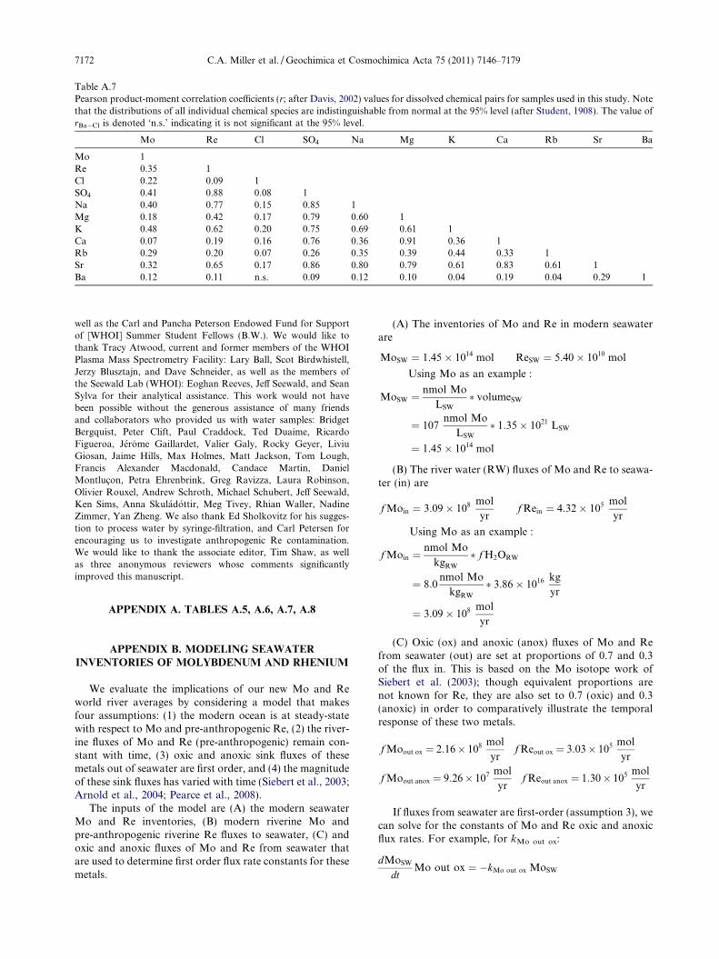
dt

Table A.7Pearson product-moment correlation coefficients (r; after Davis, 2002) values for dissolved chemical pairs for samples used in this study. Notethat the distributions of all individual chemical species are indistinguishable from normal at the 95% level (after Student, 1908). The value ofrBa�Cl is denoted ‘n.s.’ indicating it is not significant at the 95% level.

Mo Re Cl SO4 Na Mg K Ca Rb Sr Ba

Mo 1Re 0.35 1Cl 0.22 0.09 1SO4 0.41 0.88 0.08 1Na 0.40 0.77 0.15 0.85 1Mg 0.18 0.42 0.17 0.79 0.60 1K 0.48 0.62 0.20 0.75 0.69 0.61 1Ca 0.07 0.19 0.16 0.76 0.36 0.91 0.36 1Rb 0.29 0.20 0.07 0.26 0.35 0.39 0.44 0.33 1Sr 0.32 0.65 0.17 0.86 0.80 0.79 0.61 0.83 0.61 1Ba 0.12 0.11 n.s. 0.09 0.12 0.10 0.04 0.19 0.04 0.29 1

7172 C.A. Miller et al. / Geochimica et Cosmochimica Acta 75 (2011) 7146–7179

well as the Carl and Pancha Peterson Endowed Fund for Supportof [WHOI] Summer Student Fellows (B.W.). We would like tothank Tracy Atwood, current and former members of the WHOIPlasma Mass Spectrometry Facility: Lary Ball, Scot Birdwhistell,Jerzy Blusztajn, and Dave Schneider, as well as the members ofthe Seewald Lab (WHOI): Eoghan Reeves, Jeff Seewald, and SeanSylva for their analytical assistance. This work would not havebeen possible without the generous assistance of many friendsand collaborators who provided us with water samples: BridgetBergquist, Peter Clift, Paul Craddock, Ted Duaime, RicardoFigueroa, Jerome Gaillardet, Valier Galy, Rocky Geyer, LiviuGiosan, Jaime Hills, Max Holmes, Matt Jackson, Tom Lough,Francis Alexander Macdonald, Candace Martin, DanielMontluc�on, Petra Ehrenbrink, Greg Ravizza, Laura Robinson,Olivier Rouxel, Andrew Schroth, Michael Schubert, Jeff Seewald,Ken Sims, Anna Skuladottir, Meg Tivey, Rhian Waller, NadineZimmer, Yan Zheng. We also thank Ed Sholkovitz for his sugges-tion to process water by syringe-filtration, and Carl Petersen forencouraging us to investigate anthropogenic Re contamination.We would like to thank the associate editor, Tim Shaw, as wellas three anonymous reviewers whose comments significantlyimproved this manuscript.

APPENDIX A. TABLES A.5, A.6, A.7, A.8

APPENDIX B. MODELING SEAWATER

INVENTORIES OF MOLYBDENUM AND RHENIUM

We evaluate the implications of our new Mo and Reworld river averages by considering a model that makesfour assumptions: (1) the modern ocean is at steady-statewith respect to Mo and pre-anthropogenic Re, (2) the river-ine fluxes of Mo and Re (pre-anthropogenic) remain con-stant with time, (3) oxic and anoxic sink fluxes of thesemetals out of seawater are first order, and (4) the magnitudeof these sink fluxes has varied with time (Siebert et al., 2003;Arnold et al., 2004; Pearce et al., 2008).

The inputs of the model are (A) the modern seawaterMo and Re inventories, (B) modern riverine Mo andpre-anthropogenic riverine Re fluxes to seawater, (C) andoxic and anoxic fluxes of Mo and Re from seawater thatare used to determine first order flux rate constants for thesemetals.

(A) The inventories of Mo and Re in modern seawaterare

MoSW ¼ 1:45� 1014 mol ReSW ¼ 5:40� 1010 mol

Using Mo as an example :

MoSW ¼nmol Mo

LSW

� volumeSW

¼ 107nmol Mo

LSW

� 1:35� 1021 LSW

¼ 1:45� 1014 mol

(B) The river water (RW) fluxes of Mo and Re to seawa-ter (in) are

f Moin ¼ 3:09� 108 mol

yrf Rein ¼ 4:32� 105 mol

yr

Using Mo as an example :

f Moin ¼nmol Mo

kgRW

� f H2ORW

¼ 8:0nmol Mo

kgRW

� 3:86� 1016 kg

yr

¼ 3:09� 108 mol

yr

(C) Oxic (ox) and anoxic (anox) fluxes of Mo and Refrom seawater (out) are set at proportions of 0.7 and 0.3of the flux in. This is based on the Mo isotope work ofSiebert et al. (2003); though equivalent proportions arenot known for Re, they are also set to 0.7 (oxic) and 0.3(anoxic) in order to comparatively illustrate the temporalresponse of these two metals.

f Moout ox ¼ 2:16� 108 mol

yrf Reout ox ¼ 3:03� 105 mol

yr

f Moout anox ¼ 9:26� 107 mol

yrf Reout anox ¼ 1:30� 105 mol

yr

If fluxes from seawater are first-order (assumption 3), wecan solve for the constants of Mo and Re oxic and anoxicflux rates. For example, for kMo out ox:

dMoSWMo out ox ¼ �kMo out ox MoSW

Table A.8Chemical data for precipitation and mine water samples. Chemical data are listed to the last significant digit. Where the last significant digit is zero, this is indicated by a decimal point or scientificnotation. Uncertainties are as listed in Section 3. Data listed as “b.d.” were below the detection limits.

Sample Mo(nmol kg�1)

Re(pmol kg�1)

Cl(lmol kg�1)

SO4

(lmol kg�1)Na(lmol kg�1)

Mg(lmol kg�1)

Ca(lmol kg�1)

K(lmol kg�1)

Rb(nmol kg�1)

Sr(nmol kg�1)

Ba(nmol kg�1)

Precipitation, Falmouth, MAa

2004/09/18 0.080 1.41 103 33 80 10.6 7.1 4.6 b.d. b.d. 432004/09/18 0.080 0.91 23 4.9 4.3 2.20 4.6 1.4 b.d. b.d. b.d.2004/10/15 0.047 0.81 26 8.0 b.d. 2.97 7.5 3.9 b.d. b.d. 202004/12/01 0.64 1.25 204 17.0 140 19.4 7.6 5.6 b.d. b.d. 162004/12/10 0.062 0.70 26 7.2 b.d. 2.79 5.8 b.d. b.d. b.d. 332004/12/26 0.021 0.29 16.4 2.4 b.d. 1.64 7.1 b.d. b.d. b.d. 442005/01/06 0.067 1.03 9.8 4.5 b.d. 0.98 4.1 b.d. b.d. b.d. 712005/01/24 0.061 0.173 57 4.7 23 5.63 5.8 b.d. b.d. b.d. 192005/02/14 0.147 1.15 9.8 19 b.d. 1.19 5.3 b.d. b.d. b.d. 252005/02/16 0.135 5.9 440 32 320 39.9 25 19 12 b.d. 212005/02/21 0.136 1.13 31 7.9 7 3.31 3.7 b.d. b.d. b.d. 352005/02/21 b.d. 0.57 14 3.7 b.d. 1.82 3.9 b.d. b.d. b.d. b.d.2005/02/24–25 0.135 5.9 14 2.0 b.d. 2.54 6.6 b.d. b.d. b.d. b.d.2005/02/28 0.136 1.13 20 3.1 b.d. 2.53 4.7 b.d. b.d. b.d. 282005/03/?? 0.061 0.30 71 7.0 36 6.87 8.1 1.6 b.d. b.d. 482005/04/15–2005/05/10 0.023 2.4 95 16.6 65 9.1 8.8 3.1 b.d. b.d. 222005/07/08 1.28 0.35 19 7.9 b.d. 1.73 8.0 0.7 b.d. b.d. 20.2005/09/16 b.d. 0.034 1.83 1.00 b.d. 0.425 4.3 b.d. b.d. b.d. 100.2005/09/24 b.d. 0.27 71 8.5 46 7.16 6.6 3.5 b.d. b.d. 692005/09/29 0.060 2.2 360 42 280 35.4 21 b.d. 10 b.d. 17

Mine waters

Berkeley Pit, surface 0.76 11,900 710 8.0 � 104 6.7 268 11,000 90 590 b.d. 930Berkeley Pit, �76 m 0.62 1.31 � 104 550 86,000 5.1 132 15,000 2.6 270 b.d. 410Mansfeld 1 220 14,400 – – 43 4330 16,000 7.0 � 102 470 19,000 120Mansfeld 2 250 37,100 – – 2400 4650 14,000 7.0 � 102 570 33,000 150Mansfeld 3 190 16,200 – – 2.0 � 104 7070 2.0 � 104 1200 800 14,000 170

a Data for precipitation samples are the only ones corrected that have been corrected for cyclic sea salt.

Sampling locations Lat, Lon:Falmouth, MA, USA: 41.5605, �070.6154Berkeley Pit, MT, USA: 46.0167, �112.5060Mansfeld, Germany: 51.5941, �011.4547

Mo

and

Re

surface

cycling

7173

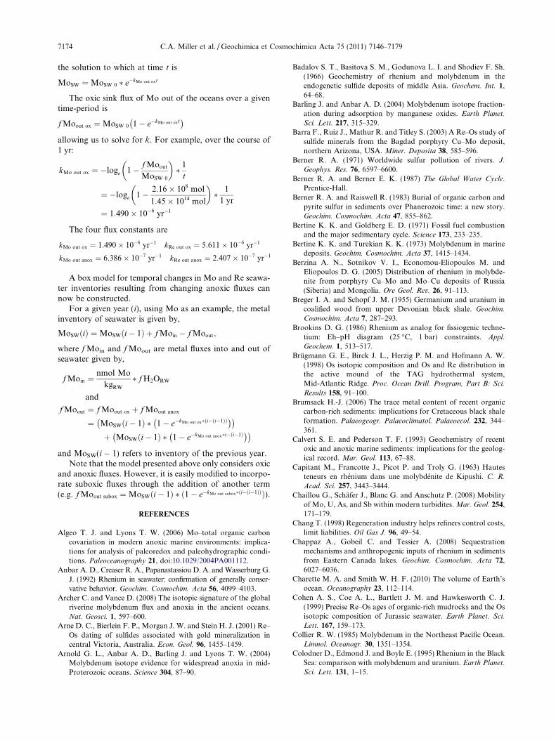
7174 C.A. Miller et al. / Geochimica et Cosmochimica Acta 75 (2011) 7146–7179

the solution to which at time t is

MoSW ¼MoSW 0 � e�kMo out ox t

The oxic sink flux of Mo out of the oceans over a giventime-period is

f Moout ox ¼MoSW 0 1� e�kMo out ox t� �

allowing us to solve for k. For example, over the course of1 yr:

kMo out ox ¼ �loge 1� f Moout

MoSW 0

� �� 1

t

¼ �loge 1� 2:16� 108 mol

1:45� 1014 mol

� �� 1

1 yr

¼ 1:490� 10�6 yr�1

The four flux constants are

kMo out ox ¼ 1:490� 10�6 yr�1 kRe out ox ¼ 5:611� 10�6 yr�1

kMo out anox ¼ 6:386� 10�7 yr�1 kRe out anox ¼ 2:407� 10�7 yr�1

A box model for temporal changes in Mo and Re seawa-ter inventories resulting from changing anoxic fluxes cannow be constructed.

For a given year (i), using Mo as an example, the metalinventory of seawater is given by,

MoSWðiÞ ¼MoSWði� 1Þ þ f Moin � f Moout;

where f Moin and f Moout are metal fluxes into and out ofseawater given by,

f Moin ¼nmol Mo

kgRW

� f H2ORW

and

f Moout ¼ f Moout ox þ f Moout anox

¼ MoSWði� 1Þ � 1� e�kMo out ox� i� i�1ð Þð Þ� �� �þ MoSWði� 1Þ � 1� e�kMo out anox�i� i�1ð Þ� �� �

and MoSW(i � 1) refers to inventory of the previous year.Note that the model presented above only considers oxic

and anoxic fluxes. However, it is easily modified to incorpo-rate suboxic fluxes through the addition of another term(e.g. f Moout subox ¼MoSWði� 1Þ � ð1� e�kMo out subox�ði�ði�1ÞÞÞ).

REFERENCES

Algeo T. J. and Lyons T. W. (2006) Mo–total organic carboncovariation in modern anoxic marine environments: implica-tions for analysis of paleoredox and paleohydrographic condi-tions. Paleoceanography 21, doi:10.1029/2004PA001112.

Anbar A. D., Creaser R. A., Papanastassiou D. A. and Wasserburg G.J. (1992) Rhenium in seawater: confirmation of generally conser-vative behavior. Geochim. Cosmochim. Acta 56, 4099–4103.

Archer C. and Vance D. (2008) The isotopic signature of the globalriverine molybdenum flux and anoxia in the ancient oceans.Nat. Geosci. 1, 597–600.

Arne D. C., Bierlein F. P., Morgan J. W. and Stein H. J. (2001) Re–Os dating of sulfides associated with gold mineralization incentral Victoria, Australia. Econ. Geol. 96, 1455–1459.

Arnold G. L., Anbar A. D., Barling J. and Lyons T. W. (2004)Molybdenum isotope evidence for widespread anoxia in mid-Proterozoic oceans. Science 304, 87–90.

Badalov S. T., Basitova S. M., Godunova L. I. and Shodiev F. Sh.(1966) Geochemistry of rhenium and molybdenum in theendogenetic sulfide deposits of middle Asia. Geochem. Int. 1,

64–68.

Barling J. and Anbar A. D. (2004) Molybdenum isotope fraction-ation during adsorption by manganese oxides. Earth Planet.

Sci. Lett. 217, 315–329.

Barra F., Ruiz J., Mathur R. and Titley S. (2003) A Re–Os study ofsulfide minerals from the Bagdad porphyry Cu–Mo deposit,northern Arizona, USA. Miner. Deposita 38, 585–596.

Berner R. A. (1971) Worldwide sulfur pollution of rivers. J.

Geophys. Res. 76, 6597–6600.

Berner R. A. and Berner E. K. (1987) The Global Water Cycle.Prentice-Hall.

Berner R. A. and Raiswell R. (1983) Burial of organic carbon andpyrite sulfur in sediments over Phanerozoic time: a new story.Geochim. Cosmochim. Acta 47, 855–862.

Bertine K. K. and Goldberg E. D. (1971) Fossil fuel combustionand the major sedimentary cycle. Science 173, 233–235.

Bertine K. K. and Turekian K. K. (1973) Molybdenum in marinedeposits. Geochim. Cosmochim. Acta 37, 1415–1434.

Berzina A. N., Sotnikov V. I., Economou-Eliopoulos M. andEliopoulos D. G. (2005) Distribution of rhenium in molybde-nite from porphyry Cu–Mo and Mo–Cu deposits of Russia(Siberia) and Mongolia. Ore Geol. Rev. 26, 91–113.

Breger I. A. and Schopf J. M. (1955) Germanium and uranium incoalified wood from upper Devonian black shale. Geochim.

Cosmochim. Acta 7, 287–293.

Brookins D. G. (1986) Rhenium as analog for fissiogenic techne-tium: Eh–pH diagram (25 �C, 1 bar) constraints. Appl.

Geochem. 1, 513–517.

Brugmann G. E., Birck J. L., Herzig P. M. and Hofmann A. W.(1998) Os isotopic composition and Os and Re distribution inthe active mound of the TAG hydrothermal system,Mid-Atlantic Ridge. Proc. Ocean Drill. Program, Part B: Sci.

Results 158, 91–100.

Brumsack H.-J. (2006) The trace metal content of recent organiccarbon-rich sediments: implications for Cretaceous black shaleformation. Palaeogeogr. Palaeoclimatol. Palaeoecol. 232, 344–

361.

Calvert S. E. and Pederson T. F. (1993) Geochemistry of recentoxic and anoxic marine sediments: implications for the geolog-ical record. Mar. Geol. 113, 67–88.

Capitant M., Francotte J., Picot P. and Troly G. (1963) Hautesteneurs en rhenium dans une molybdenite de Kipushi. C. R.

Acad. Sci. 257, 3443–3444.

Chaillou G., Schafer J., Blanc G. and Anschutz P. (2008) Mobilityof Mo, U, As, and Sb within modern turbidites. Mar. Geol. 254,

171–179.

Chang T. (1998) Regeneration industry helps refiners control costs,limit liabilities. Oil Gas J. 96, 49–54.

Chappaz A., Gobeil C. and Tessier A. (2008) Sequestrationmechanisms and anthropogenic inputs of rhenium in sedimentsfrom Eastern Canada lakes. Geochim. Cosmochim. Acta 72,

6027–6036.

Charette M. A. and Smith W. H. F. (2010) The volume of Earth’socean. Oceanography 23, 112–114.

Cohen A. S., Coe A. L., Bartlett J. M. and Hawkesworth C. J.(1999) Precise Re–Os ages of organic-rich mudrocks and the Osisotopic composition of Jurassic seawater. Earth Planet. Sci.

Lett. 167, 159–173.

Collier R. W. (1985) Molybdenum in the Northeast Pacific Ocean.Limnol. Oceanogr. 30, 1351–1354.

Colodner D., Edmond J. and Boyle E. (1995) Rhenium in the BlackSea: comparison with molybdenum and uranium. Earth Planet.

Sci. Lett. 131, 1–15.

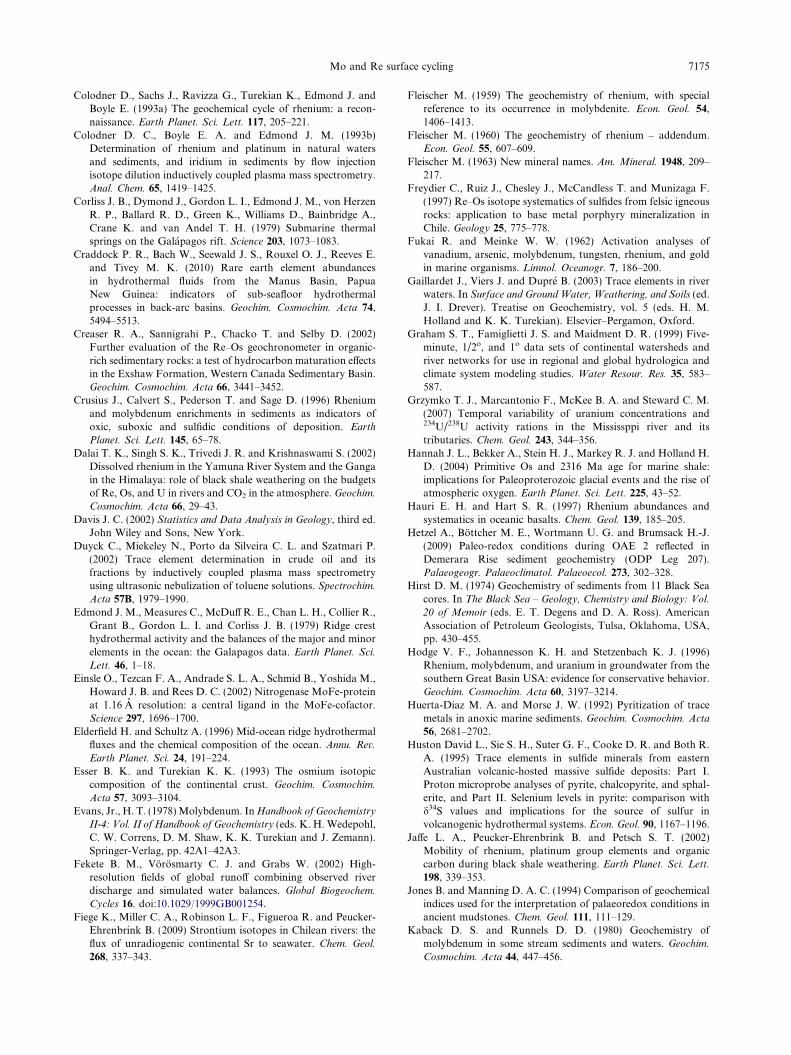
Mo and Re surface cycling 7175

Colodner D., Sachs J., Ravizza G., Turekian K., Edmond J. andBoyle E. (1993a) The geochemical cycle of rhenium: a recon-naissance. Earth Planet. Sci. Lett. 117, 205–221.

Colodner D. C., Boyle E. A. and Edmond J. M. (1993b)Determination of rhenium and platinum in natural watersand sediments, and iridium in sediments by flow injectionisotope dilution inductively coupled plasma mass spectrometry.Anal. Chem. 65, 1419–1425.

Corliss J. B., Dymond J., Gordon L. I., Edmond J. M., von HerzenR. P., Ballard R. D., Green K., Williams D., Bainbridge A.,Crane K. and van Andel T. H. (1979) Submarine thermalsprings on the Galapagos rift. Science 203, 1073–1083.

Craddock P. R., Bach W., Seewald J. S., Rouxel O. J., Reeves E.and Tivey M. K. (2010) Rare earth element abundancesin hydrothermal fluids from the Manus Basin, PapuaNew Guinea: indicators of sub-seafloor hydrothermalprocesses in back-arc basins. Geochim. Cosmochim. Acta 74,

5494–5513.

Creaser R. A., Sannigrahi P., Chacko T. and Selby D. (2002)Further evaluation of the Re–Os geochronometer in organic-rich sedimentary rocks: a test of hydrocarbon maturation effectsin the Exshaw Formation, Western Canada Sedimentary Basin.Geochim. Cosmochim. Acta 66, 3441–3452.

Crusius J., Calvert S., Pederson T. and Sage D. (1996) Rheniumand molybdenum enrichments in sediments as indicators ofoxic, suboxic and sulfidic conditions of deposition. Earth

Planet. Sci. Lett. 145, 65–78.

Dalai T. K., Singh S. K., Trivedi J. R. and Krishnaswami S. (2002)Dissolved rhenium in the Yamuna River System and the Gangain the Himalaya: role of black shale weathering on the budgetsof Re, Os, and U in rivers and CO2 in the atmosphere. Geochim.

Cosmochim. Acta 66, 29–43.

Davis J. C. (2002) Statistics and Data Analysis in Geology, third ed.John Wiley and Sons, New York.

Duyck C., Miekeley N., Porto da Silveira C. L. and Szatmari P.(2002) Trace element determination in crude oil and itsfractions by inductively coupled plasma mass spectrometryusing ultrasonic nebulization of toluene solutions. Spectrochim.

Acta 57B, 1979–1990.

Edmond J. M., Measures C., McDuff R. E., Chan L. H., Collier R.,Grant B., Gordon L. I. and Corliss J. B. (1979) Ridge cresthydrothermal activity and the balances of the major and minorelements in the ocean: the Galapagos data. Earth Planet. Sci.

Lett. 46, 1–18.

Einsle O., Tezcan F. A., Andrade S. L. A., Schmid B., Yoshida M.,Howard J. B. and Rees D. C. (2002) Nitrogenase MoFe-proteinat 1.16 A resolution: a central ligand in the MoFe-cofactor.Science 297, 1696–1700.

Elderfield H. and Schultz A. (1996) Mid-ocean ridge hydrothermalfluxes and the chemical composition of the ocean. Annu. Rev.

Earth Planet. Sci. 24, 191–224.

Esser B. K. and Turekian K. K. (1993) The osmium isotopiccomposition of the continental crust. Geochim. Cosmochim.

Acta 57, 3093–3104.

Evans, Jr., H. T. (1978) Molybdenum. In Handbook of Geochemistry

II-4: Vol. II of Handbook of Geochemistry (eds. K. H. Wedepohl,C. W. Correns, D. M. Shaw, K. K. Turekian and J. Zemann).Springer-Verlag, pp. 42A1–42A3.

Fekete B. M., Vorosmarty C. J. and Grabs W. (2002) High-resolution fields of global runoff combining observed riverdischarge and simulated water balances. Global Biogeochem.

Cycles 16. doi:10.1029/1999GB001254.

Fiege K., Miller C. A., Robinson L. F., Figueroa R. and Peucker-Ehrenbrink B. (2009) Strontium isotopes in Chilean rivers: theflux of unradiogenic continental Sr to seawater. Chem. Geol.

268, 337–343.

Fleischer M. (1959) The geochemistry of rhenium, with specialreference to its occurrence in molybdenite. Econ. Geol. 54,

1406–1413.

Fleischer M. (1960) The geochemistry of rhenium – addendum.Econ. Geol. 55, 607–609.

Fleischer M. (1963) New mineral names. Am. Mineral. 1948, 209–

217.

Freydier C., Ruiz J., Chesley J., McCandless T. and Munizaga F.(1997) Re–Os isotope systematics of sulfides from felsic igneousrocks: application to base metal porphyry mineralization inChile. Geology 25, 775–778.

Fukai R. and Meinke W. W. (1962) Activation analyses ofvanadium, arsenic, molybdenum, tungsten, rhenium, and goldin marine organisms. Limnol. Oceanogr. 7, 186–200.

Gaillardet J., Viers J. and Dupre B. (2003) Trace elements in riverwaters. In Surface and Ground Water, Weathering, and Soils (ed.J. I. Drever). Treatise on Geochemistry, vol. 5 (eds. H. M.Holland and K. K. Turekian). Elsevier–Pergamon, Oxford.

Graham S. T., Famiglietti J. S. and Maidment D. R. (1999) Five-minute, 1/2o, and 1o data sets of continental watersheds andriver networks for use in regional and global hydrologica andclimate system modeling studies. Water Resour. Res. 35, 583–

587.

Grzymko T. J., Marcantonio F., McKee B. A. and Steward C. M.(2007) Temporal variability of uranium concentrations and234U/238U activity rations in the Mississppi river and itstributaries. Chem. Geol. 243, 344–356.

Hannah J. L., Bekker A., Stein H. J., Markey R. J. and Holland H.D. (2004) Primitive Os and 2316 Ma age for marine shale:implications for Paleoproterozoic glacial events and the rise ofatmospheric oxygen. Earth Planet. Sci. Lett. 225, 43–52.

Hauri E. H. and Hart S. R. (1997) Rhenium abundances andsystematics in oceanic basalts. Chem. Geol. 139, 185–205.

Hetzel A., Bottcher M. E., Wortmann U. G. and Brumsack H.-J.(2009) Paleo-redox conditions during OAE 2 reflected inDemerara Rise sediment geochemistry (ODP Leg 207).Palaeogeogr. Palaeoclimatol. Palaeoecol. 273, 302–328.

Hirst D. M. (1974) Geochemistry of sediments from 11 Black Seacores. In The Black Sea – Geology, Chemistry and Biology: Vol.

20 of Memoir (eds. E. T. Degens and D. A. Ross). American

Association of Petroleum Geologists, Tulsa, Oklahoma, USA,

pp. 430–455.

Hodge V. F., Johannesson K. H. and Stetzenbach K. J. (1996)Rhenium, molybdenum, and uranium in groundwater from thesouthern Great Basin USA: evidence for conservative behavior.Geochim. Cosmochim. Acta 60, 3197–3214.

Huerta-Diaz M. A. and Morse J. W. (1992) Pyritization of tracemetals in anoxic marine sediments. Geochim. Cosmochim. Acta

56, 2681–2702.

Huston David L., Sie S. H., Suter G. F., Cooke D. R. and Both R.A. (1995) Trace elements in sulfide minerals from easternAustralian volcanic-hosted massive sulfide deposits: Part I.Proton microprobe analyses of pyrite, chalcopyrite, and sphal-erite, and Part II. Selenium levels in pyrite: comparison withd34S values and implications for the source of sulfur involcanogenic hydrothermal systems. Econ. Geol. 90, 1167–1196.

Jaffe L. A., Peucker-Ehrenbrink B. and Petsch S. T. (2002)Mobility of rhenium, platinum group elements and organiccarbon during black shale weathering. Earth Planet. Sci. Lett.

198, 339–353.

Jones B. and Manning D. A. C. (1994) Comparison of geochemicalindices used for the interpretation of palaeoredox conditions inancient mudstones. Chem. Geol. 111, 111–129.

Kaback D. S. and Runnels D. D. (1980) Geochemistry ofmolybdenum in some stream sediments and waters. Geochim.

Cosmochim. Acta 44, 447–456.

7176 C.A. Miller et al. / Geochimica et Cosmochimica Acta 75 (2011) 7146–7179

Kemp D. B., Coe A. L., Cohen A. S. and Schwark L. (2005)Astronomical pacing of methane release in the Early Jurassicperiod. Nature 437, 396–399.

Kharkar D. P., Turekian K. K. and Bertine K. K. (1968) Streamsupply of dissolved silver, molybdenum, antimony, selenium,chromium, cobalt, rubidium and cesium to the oceans.Geochim. Cosmochim. Acta 32, 285–298.

Kim J. and Rees D. C. (1992) Structural models for the metalcenters in the nitrogenase molybdenum-iron protein. Science

257, 1677–1682.

Kirk J., Ruiz J., Chesley J., Titley S. and Walshe J. (2001) Adetrital model for the origin of gold and sulfides in theWitwatersrand basin based on Re–Os isotopes. Geochim.

Cosmochim. Acta 65, 2149–2159.

Kirk J., Ruiz J., Chesley J., Walshe J. and England G. (2002) Amajor Archean, gold- and crust-forming event in the KaapvaalCraton, South Africa. Science 297, 1856–1858.

Klinkhammer G. P. and Palmer M. R. (1991) Uranium in theoceans: where it goes and why. Geochim. Cosmochim. Acta 55,

1799–1806.

Koide M., Hodge V., Yang J. S. and Goldberg E. D. (1987)Determination of rhenium in marine waters and sediments bygraphite furnace atomic absorption spectrometry. Anal. Chem.

59, 1802–1805.

Koide M., Hodge V. F., Yang J. S., Stallard M., Goldberg E. G.,Calhoun J. and Bertine K. K. (1986) Some comparative marinechemistries of rhenium, gold, silver and molybdenum. Appl.

Geochem. 1, 705–714.

Korzhinski M. A., Tkachenko S. I., Shmulovich K. I., Taran Y. A.and Steinberg G. S. (1994) Discovery of a pure rhenium mineralat Kudriavy volcano. Nature 369, 51–52.

Large R. R., Danyushevsky L., Hollit C., Maslennikov V., MeffreS., Gilbert S., Bull S., Scott R., Emsbo P., Thomas H., Singh B.and Foster J. (2009) Gold and trace element zonation in pyriteusing a laser imaging technique: implications for the timing ofgold in orogenic and Carlin-style sediment-hosted deposits.Econ. Geol. 104, 635–668.

Le Riche H. H. (1959) The distribution of certain trace elements inthe Lower Lias of southern England. Geochim. Cosmochim.

Acta 16, 101–122.

Łetowski F., Serkies J. and Niemiec J. (1966) Application ofpotential-pH diagrams for determination of the occurrenceforms of trace elements in some economic mineral deposits.Econ. Geol. 61, 1272–1279.

Leybourne M. I. and Cameron E. M. (2008) Source, transport, andfate of rhenium, selenium, molybdenum, arsenic, and copper ingroundwater associated with porphyry-Cu deposits, AtacamaDesert, Chile. Chem. Geol. 247, 208–228.

Ling H.-F., Gao J. F., Zhao K.-D., Jiang S.-Y. and Ma D.-S.(2005) Comment on “Molybdenum isotope evidence for wide-spread anoxia in Mid-Proterozoic oceans”. Science 309, 1017c.

Lipinski M., Warning B. and Brumsack H.-J. (2003) Tracemetal signatures of Jurassic/Cretaceous black shales fromthe Norwegian Shelf and the Barents Sea. Palaeogeogr.

Palaeoclimatol. Palaeoecol. 190, 459–475.

Liu G., Chou C.-L., Peng Z. and Yang G. (2008) Abundances andisotopic compositions of rhenium and osmium in pyrite samplesfrom Huaibei coalfield, Anhui, China. Int. J. Earth Sci. 97, 617–

621.

Livingstone D. A. (1963) Chemical composition of rivers and lakes.In Data of Geochemistry, 6th ed. (ed. M. Fleischer). UnitedStates Geological Survey Professional Paper. United StatesGovernment, Department of the Interior. G1–G64.

Manheim F. T. (1972) Red Sea geochemistry. Init. Rep. Deep Sea

Drill. Project 23, 975–998.

Manheim F. T. and Landergren S. (1978) Molybdenum. InHandbook of Geochemistry II-4: Vol. II of Handbook of

Geochemistry (eds. K. H. Wedepohl, C. W. Correns, D. M.Shaw, K. K. Turekian and J. Zemann). Springer-Verlag, pp.42B1–42O2.

Manheim F. T. and Siems D. E. (1972) Chemical analyses of RedSea sediments. Init. Rep. Deep Sea Drill. Project 23, 923–938.

Mao J., Du A., Seltmann R. and Yu J. (2003) Re–Os ages for theShamika porphyry Mo deposit and the Lipovy Log rare metalpegmatite, central Urals, Russia. Miner. Deposita 38, 251–257.

Mao J., Wang Y., Lehmann B., Yu J., Du A., Mei Y., Li Y., ZangW., Stein H. J. and Zhou T. (2006) Molybdenite Re–Os andalbite 40Ar/39Ar dating of Cu–Au–Mo and magnetite porphyrysystems in the Yangtze River valley and metallogenic implica-tions. Ore Geol. Rev. 29, 307–324.

Markey R., Stein H. and Morgan J. (1998) Highly precise Re–Osdating for molybdenite using alkaline fusion and NTIMS.Talanta 45, 935–946.

Maslennikov V. V., Maslennikova S. P., Large R. R. andDanyushevsky L. V. (2009) Study of trace element zonationin vent chimneys from the Silurian Yaman-Kasy volcanic-hosted massive sulfide deposit (southern Urals, Russia) usinglaser ablation-inductively coupled plasma mass spectrometry(LA-ICPMS). Econ. Geol. 104, 1111–1141.

Mason B. and Moore C. B. (1982) Principles of Geochemistry. JohnWiley and Sons.

Mathur R., Ruiz J. and Munizaga F. (2000) Relationship betweencopper tonnage of Chilean base-metal porphyry deposits andOs isotope ratios. Geology 28, 555–558.

Mathur R., Ruiz J. and Tornos F. (1999) Age and sources of theore at Tharsis and Rio Tinto, Iberian Pyrite Belt, from Re–Osisotopes. Miner. Deposita 34, 790–793.

Mathur R., Titley S., Ruiz J., Gibbins S. and Friehauf K. (2005) ARe–Os study of sedimentary rocks and copper–gold ores fromErtsberg District, West Papua, Indonesia. Ore Geol. Rev. 26,

207–226.

McArthur J. M., Donovan D. T., Thirlwall M. F., Fouke B. W.and Mattey D. (2000) Strontium isotope profile of the earlyToarcian (Jurassic) oceanic anoxic event, the duration ofammonite biozones, and belemnite palaeotemperatures. Earth

Planet. Sci. Lett. 179, 269–285.

McCandless T. E., Ruiz J. and Campbell A. R. (1993) Rheniumbehavior in molybdenite in hypogene and near surface envi-ronments: implications for Re–Os geochronometry. Geochim.

Cosmochim. Acta 57, 889–905.

McLennan S. M. (2001) Relationships between the traceelement composition of sedimentary rocks and upper continen-tal crust. Geochem. Geophys. Geosyst. 2. doi:10.1029/2000

GC000109.

Meisel T. and Stotter V. (2007) Identifying the sources of PGE, Reand Sb in road dust and soils along highways. Geochim.

Cosmochim. Acta Suppl. 71, A650.

Metz S. and Trefry J. H. (2000) Chemical and mineralogicalinfluences on concentrations of trace metals in hydrothermalfluids. Geochim. Cosmochim. Acta 64, 2267–2279.

Meybeck M. (1979) Concentration des eaux fluviales en elementsmajeurs et apports en solution aux oceans. Rev. Geol. Dyn.

Geogr. Phys. 21, 215–246.

Meybeck M. (1988) How to establish and use world budgets ofriverine material. In Physical and Chemical Weathering in

Geochemical Cycles (eds. A. Lerman and M. Meybeck). Kluwer

Academic Publishers, pp. 247–272.

Meybeck M. and Helmer R. (1989) The quality of rivers: frompristine stage to global pollution. Palaeogeogr. Palaeoclimatol.

Palaeoecol. 75, 283–309.

Mo and Re surface cycling 7177

Meybeck M. and Ragu A. (1995) River discharges to the oceans: anassessment of suspended solids, major ions and nutrients.Technical Report, United Nations Environment Programme.

Miller C. A. (2004) Re–Os dating of algal laminites: reductionenrichment of metals in the sedimentary environment and newgeoporphyrins. Master’s thesis, University of Saskatchewan,Saskatoon.

Miller C. A. (2009) Surface-cycling of rhenium and its isotopes.Ph.D. thesis, Massachusetts Institute of Technology, WoodsHole Oceanographic Institution.

Millero F. J. and Poisson A. (1981) International one-atmosphereequation of state for seawater. Deep Sea Res. 28A, 625–629.

Mitchell R. H., Laflamme J. H. G. and Cabri L. J. (1989) Rheniumsulphide from the Coldwell complex, northwestern Ontario,Canada. Mineral. Mag. 53, 635–637.

Montgomery R. B. (1958) Water characteristics of Atlantic Oceanand of world ocean.. Deep Sea Res. 5, 134–148.

Morachevskii D. E. and Nechaeva A. A. (1960) Characteristics ofmigration of rhenium from molybdenites. Geochemistry 6, 648–

651.

Morelli R. M., Creaser R. A., Selby D., Kelley K. D., Leach D. L.and King A. R. (2004) Re–Os sulfide geochronology of the RedDog sediment-hosted Zn–Pb–Ag deposit, Brooks Range,Alaska. Econ. Geol. 99, 1569–1576.

Morelli R. M., Creaser R. A., Selby D., Kontak D. J. and HorneR. J. (2005) Rhenium–osmium geochronology of arsenopyritein Meguma Group gold deposits, Meguma terrane, NovaScotia, Canada: evidence for multiple gold-mineralizing events.Econ. Geol. 100, 1229–1242.

Morelli R., Creaser R. A., Seltmann R., Stuart F. M., Selby D. andGraupner T. (2007) Age and source constraints for the giantMuruntau gold deposit, Uzbekistan, from coupled Re–Os–Heisotopes in arsenopyrite. Geology 35, 795–798.

Morford J. L. and Emerson S. (1999) The geochemistry of redoxsensitive trace metals in sediments. Geochim. Cosmochim. Acta

63, 1735–1750.

Morford J. L., Martin W. R., Kalnejais L. H., Franc�ois R.,Bothner M. and Karle I.-M. (2007) Insights on geochemicalcycling of U, Re and Mo from seasonal sampling in BostonHarbor, Massachusetts, USA. Geochim. Cosmochim. Acta 71,

895–917.

Morgan J. W., Golightly D. W. and Dorrzapf Jr., A. F. (1991)Methods for the separation of rhenium, osmium and molyb-denum applicable to isotope geochemistry. Talanta 38, 259–265.

Morris A. W. (1975) Dissolved molybdenum and vanadium in thenortheast Atlantic Ocean. Deep Sea Res. 22, 49–54.

Morris A. W. and Riley J. P. (1966) The bromide/chlorinity andsulphate/chlorinity ratio in sea water. Deep Sea Res. 13, 699–

705.

Morris D. F. C. and Short E. L. (1966) Minerals of rhenium.Mineral. Mag. 35(274), 871–873.

Moyse B. M. (2000) Process, catalyst choices key to producing 30-ppm sulfur fuels. Oil Gas J. 98, 72–74.

Nagler Th. F., Siebert C., Luschen H. and Bottcher M. E. (2005)Sedimentary Mo isotope record across the Holocene fresh-brackish water transition of the Black Sea. Chem. Geol. 219,

283–295.

Nesheim L., Gautneb H. and Myhr K. (1997) Plant uptake ofsulphur and trace elements from pyrite applied on grassland.Acta Agric. Scand. B: Soil Plant Sci. 47, 135–141.

Neubert N., Heri A. R., Voegelin A. R., Nagler T. F., SchluneggerF. and Villa I. M. (2011) The molybdenum isotopic composi-tion in river water: constraints from small catchments. Earth

Planet. Sci. Lett. 304, 180–190.

Neubert N., Nagler T. F. and Bottcher M. E. (2008) Sulfiditycontrols molybdenum isotope fractionation into euxinic

sediments: evidence from the modern Black Sea. Geology 36,

775–778.

Noddack I. and Noddack W. (1931) Die Geochemie des Rheniums.Z. Phys. Chem. 154A, 207–244.

Noddack W., Tacke I. and Berg O. (1925) Zwei neue Elemente derMangangruppe. Sitzung der physikalisch-mathematischen Klasse

11, 400–409.

Patterson J. H., Ramsden A. R., Dale L. S. and Fardy J. J. (1986)Geochemistry and mineralogical residences of trace elements inoil shales from Julia Creek, Queensland, Australia. Chem. Geol.

55, 1–16.

Pearce C. R., Burton K. W. and Pogge von Strandmann P. A. E.(2010) Molybdenum isotope behaviour accompanyingweathering and riverine transport in a basaltic terrain. Earth

Planet. Sci. Lett. 295, 104–114.

Pearce C. R., Cohen A. S., Coe A. L. and Burton K. W. (2008)Molybdenum isotope evidence for global ocean anoxia coupledwith perturbations to the carbon cycle during the EarlyJurassic. Geology 36, 231–234.

Petersen R. G., Hamilton J. C. and Myers A. T. (1959) Anoccurrence of rhenium associated with uraninite in CoconinoCounty, Arizona. Econ. Geol. 54, 254–267.

Peucker-Ehrenbrink B. (2009) Land2Sea database of river drainagebasin sizes, annual water discharges, and suspended sedimentfluxes. Geochem. Geophys. Geosyst. 10. doi:10.1029/2008

GC002356.

Peucker-Ehrenbrink B. and Hannigan R. E. (2000) Effects of blackshale weathering on the mobility of rhenium and platinumgroup elements. Geology 28, 475–478.

Peucker-Ehrenbrink B. and Jahn B.-m. (2001) Rhenium–osmiumisotope systematics and platinum group element concentra-tions: loess and the upper continental crust. Geochem. Geophys.

Geosyst. 2. doi:10.1029/2001GC000172.

Peucker-Ehrenbrink B. and Miller M. W. (2007) Quantitativebedrock geology of the continents and large-scale drainageregions. Geochem. Geophys. Geosyst. 8. doi:10.1029/2006

GC001544.

Pilipchuk M. F. and Volkov I. I. (1974) Behavior of molybdenumin processes of sediment formation. In The Black Sea – Geology,

Chemistry and Biology: Vol. 20 of Memoir (eds. E. T. Degensand D. A. Ross). American Association of Petroleum

Geologists, Tulsa, Oklahoma, USA, pp. 542–553.

Poplavko E. M., Ivanov V. V., Karasik T. G., Miller A. D.,Orekhov V. S., Taliyev S. D., Tarkhov Y. A. and Fadeyeva V.A. (1974) On the concentration of rhenium in petroleum,petroleum bitumens, and oil shales. Geochem. Int. 11, 969–972.

Poulson R. L., Siebert C., McManus J. and Berelson W. M. (2006)Authigenic molybdenum isotope signatures in marine sedi-ments. Geology 34, 617–620.

Power M. R., Pirrie D., Jedwab J. and Stanley C. J. (2004)Platinum-group element mineralization in an As-rich magmaticsulphide system, Talnotry, southwest Scotland. Mineral. Mag.

68, 395–411.

Quinby-Hunt M. S. and Wilde P. (1996) Chemical depositionalenvironments of calcic marine black shales. Econ. Geol. 91, 4–

13.

Rahaman W. and Singh S. K. (2010) Rhenium in rivers andestuaries of India: sources, transport and behaviour. Mar.

Chem. 118, 1–10.

Raiswell R. and Plant J. (1980) The incorporation of trace elementsinto pyrite during diagenesis of black shales, Yorkshire,England. Econ. Geol. 75, 684–699.

Ravizza G., Martin C. E., German C. G. and Thompson G. (1996)Os isotopes as tracers in seafloor hydrothermal systems:metalliferous deposits from the TAG hydrothermal area,26�N Mid-Alantic Ridge. Earth Planet. Sci. Lett. 138, 105–119.

7178 C.A. Miller et al. / Geochimica et Cosmochimica Acta 75 (2011) 7146–7179

Ravizza G. and Turekian K. K. (1989) Application of the187Re–187Os system to black shale geochronometry. Geochim.

Cosmochim. Acta 53, 3257–3262.

Ravizza G., Turekian K. K. and Hay B. J. (1991) The geochemistryof rhenium and osmium in recent sediments from the Black Sea.Geochim. Cosmochim. Acta 55, 3741–3752.

Rayleigh (1896) Theoretical considerations respecting the separa-tion of gases by diffusion and similar processes. Philos. Mag. 42,

493–498.

Rodhe H. (1992) Modeling biogeochemical cycles. In Global

Biogeochemical Cycles (eds. S. S. Butcher, R. J. Charlson, G.H. Orians and G. V. Wolfe). Academic Press, pp. 55–72, Ch. 4.

Rosman K. J. R. and Taylor P. D. P. (1998) Isotopic compositionsof the elements 1997. Pure Appl. Chem. 70, 217–235.

Roy-Barman M. and Allegre C. J. (1994) 187Os/186Os ratios ofmid-ocean ridge basalts and abyssal peridotites. Geochim.

Cosmochim. Acta 58, 5043–5054.

Rubey W. R. (1951) Geologic history of sea water. Geol. Soc. Am.

Bull. 62, 1111–1148.

Scheiderich K., Helz G. R. and Walker R. J. (2010) Century-longrecord of Mo isotopic composition in sediments of a seasonallyanoxic estuary (Chesapeake Bay). Earth Planet. Sci. Lett. 289,

189–197.

Selby D. and Creaser R. A. (2001) Re–Os geochronology andsystematics in molybdenite from the Endako porphyry molyb-denum deposit, British Columbia, Canada. Econ. Geol. 96, 197–

204.

Selby D. and Creaser R. A. (2005) Direct radiometric dating ofhydrocarbon deposits using rhenium–osmium isotopes. Science

308, 1293–1295.

Selby D., Creaser R. A. and Fowler M. G. (2007a) Re–Oselemental and isotopic stematics in crude oils. Geochim.

Cosmochim. Acta 71, 378–386.

Selby D., Creaser R. A., Stein H. J., Markey R. J. and Hannah J.L. (2007b) Assessment of the 187Re decay constant by crosscalibration of Re–Os molybdenite and U–Pb zircon chronom-eters in magmatic ore systems. Geochim. Cosmochim. Acta 71,

1999–2013.

Seyfried, Jr., W. E. (1987) Experimental and theoretical constraintson hydrothermal alteration processes at mid-ocean ridges.Annu. Rev. Earth Planet. Sci. 15, 317–335.

Seyfried, Jr., W. E. and Mottl M. J. (1982) Hydrothermalalteration of basalt by seawater under seawater-dominatedconditions. Geochim. Cosmochim. Acta 46, 985–1002.

Siebert C., Nagler T. F., von Blanckenburg F. and Kramers J. D.(2003) Molybdenum isotope records as a potential new proxyfor paleoceanography. Earth Planet. Sci. Lett. 211, 159–171.

Spears D. A., Manzanares-Papayanopoulos L. I. and Booth C. A.(1999) The distribution and origin of trace elements in a UKcoal: the importance of pyrite. Fuel 78, 1671–1677.

Stein H. J., Markey R. J., Morgan J. W., Hannah J. L. andSchersten A. (2001) The remarkable Re–Os geochronometer inmolybdenite: how and why it works. Terra Nova 13, 479–486.

Stein H. J., Morgan J. W. and Schersten A. (2000) Re–Os dating oflow-level highly radiogenic (LLHR) sulfides: the Harnas golddeposit, southwest Sweden, records continental-scale tectonicevents. Econ. Geol. 95, 1657–1671.

Stein H. J., Sunblad K., Markey R. J., Morgan J. W. and MotuzaG. (1998) Re–Os ages for Archean molybdenite and pyrite,Kuittila-Kivisuo, Finland and Proterozoic molybdenite,Kabeliai, Lithuania: testing the chronometer in a metamorphicand metasomatic setting. Miner. Deposita 33, 329–345.

Student (1908) The probable error of a mean. Biometrika 6, 1–25.

Sugawara K., Okabe S. and Tanka M. (1961) Geochemistry ofmolybdenum in natural waters (II). J. Earth Sci. Nagoya Univ.

9, 114–128.

Sun W., Bennett V. C., Eggins S. M., Kamenetsky V. S. andArculus R. J. (2003a) Enhanced mantle-to-crust rheniumtransfer in undegassed arc magmas. Nature 422, 294–297.

Sun W., Xie Z., Chen J., Zhang X., Chai Z., Du A., Zhao J., ZhangC. and Zhou T. (2003b) Os–Os dating of copper and molyb-denum deposits along the middle and lower reaches of theYangtze River, China. Econ. Geol. 98, 175–180.

Takahashi Y., Uruga T., Suzuki K., Tanida H., Terada Y. andHattori K. H. (2007) An atomic level study of rhenium andradiogenic osmium in molybdenite. Geochim. Cosmochim. Acta

71, 5180–5190.

Terada K., Osaki S., Ishihara S. and Kiba T. (1971) Distribution ofrhenium in molybdenites from Japan. Geochem. J. 4, 123–141.

Trefry J. H., Butterfield D. B., Metz S., Massoth G. J., Trocine R.P. and Feely R. A. (1994) Trace metals in hydrothermalsolutions from Cleft segment on the southern Juan de FucaRidge. J. Geophys. Res. 99, 4925–4935.

Tribovillard N., Algeo T. J., Lyons T. and Riboulleau A. (2006)Trace metals as paleoredox and paleoproductivity proxies: anupdate. Chem. Geol. 232, 12–32.

Tribovillard N., Lyons T. W., Riboulleau A. and Bout-RoumazeillesV. (2008) A possible capture of molybdenum during earlydiagenesis of dysoxic sediments. Bull. Soc. Geol. France 179,

3–12.

Tuit C. B. (2003) The marine biogeochemistry of molybdenum.Ph.D. thesis, Massachusetts Institute of Technology, WoodsHole Oceanographic Institution.

Turgeon S. and Brumsack H.-J. (2006) Anoxic vs dysoxic eventsreflected in sediment geochemistry during the Cenomanian–Turonian Boundary Event (Cretaceous) in the Umbria–MarcheBasin of central Italy. Chem. Geol. 234, 321–339.

Tuttle M. L. W., Breit G. N., Goldhaber M. B. (2003). Geochem-ical data from New Albany Shale, Kentucky: a study of metalmobility during weathering of black shales. U.S. GeologicalSurvey Open-File Report 03–207, pp. 1–57.

Tuttle M. L. W., Breit G. N. and Goldhaber M. B. (2009)Weathering of the New Albany Shale, Kentucky: II. Redistri-bution of minor and trace elements. Appl. Geochem. 24, 1565–

1578.

Vine J. D., Tourtelot E. B. and Keith J. R. (1969) Elementdistribution in some trough and platform types of black shalesand associated rocks. U.S. Geological Survey Bulletin 1214-H,H1–H38.

Volborth A., Tarkian M., Stumpfl E. F. and Housley R. M. (1986)A survey of the Pd–Pt mineralization along the 35-km strike ofthe J-M Reef, Stillwater Complex, Montana. Can. Mineral. 24,

329–346.

Volkov I. I. and Fomina L. S. (1974) Influence of organic materialand processes of sulfide formation on distribution of some traceelements in deep-water sediments of Black Sea. In The Black

Sea – Geology, Chemistry and Biology: Vol. 20 of Memoir (eds.E. T. Degens and D. A. Ross). American Association of

Petroleum Geologists, Tulsa, Oklahoma, USA, pp. 456–476.

Walker J. C. G., Hays P. B. and Kasting J. F. (1981) A negativefeedback mechanism for the long-term stabilization of Earth’ssurface temperature. J. Geophys. Res. 86, 9776–9782.

Wedepohl K. H. (1964) Untersuchungen am Kupferschiefer inNordwestdeutschland; Ein Beitrag zur Deutung der Genesebituminoser Sedimente. Geochim. Cosmochim. Acta 28, 305–

364.

Wheat C. G., Mottl M. J. and Rudnicki M. (2002) Traceelement and REE composition of a low-temperature ridge-flank hydrothermal spring. Geochim. Cosmochim. Acta 66,

3693–3705.

Whittaker E. J. W. and Muntus R. (1970) Ionic radii for use ingeochemistry. Geochim. Cosmochim. Acta 34, 945–956.

Mo and Re surface cycling 7179

Xiong Y. and Wood S. A. (1999) Experimental determination ofthe solubility of ReO2 and the dominant oxidation state ofrhenium in hydrothermal solutions. Chem. Geol. 158, 245–256.

Xiong Y. and Wood S. A. (2001) Hydrothermal transport anddeposition of rhenium under subcritical conditions (up to200 �C) in light of experimental studies. Econ. Geol. 96, 1429–

1444.

Xiong Y. and Wood S. A. (2002) Experimental determination ofthe hydrothermal solubility of ReS2 and the Re–ReO2 bufferassemblage and transport of rhenium under supercriticalconditions. Geochem. Trans. 3, 1–10.

Yang J. S. (1991) High rhenium enrichment in brown algae: abiological sink of rhenium in the sea? Hydrobiologia 211, 165–

170.

Zhang J., Ren D., Zheng C., Zeng R., Chou C.-L. and Liu J. (2002)Trace element abundances in major minerals of Late Permian

coals from southwestern Guizhou province, China. Int. J. Coal

Geol. 53, 55–64.

Zhang L., Xiao W., Qin K., Qu W. and Du A. (2005) Re–Osisotopic dating of molybdenite and pyrite in the Baishan Mo–Re deposit, eastern, Tianshan NW China, and its geologicalsignificance. Miner. Deposita 39, 960–969.

Zobrist J. and Stumm W. (1981) Chemical dynamics of the Rhinecatchment area in Switzerland, extrapolation to the ‘pristine’Rhine River input to the ocean. In River Inputs to Ocean

Systems (eds. J. M. Martin, J. D. Burton and D. Eisma).UNEP/UNESCO/IOC/SCOR, United Nations, New York, pp.

52–63.

Associate editor: Timothy J. Shaw