rc-1535 - development of new test procedures for · pdf filemeasuring fine and coarse...

FINAL REPORT DEVELOPMENT OF NEW TEST PROCEDURES FOR MEASURING FINE AND COARSE AGGREGATE SPECIFIC GRAVITIES

PI: Zhanping You, Ph.D., P.E. DEPARTMENT OF CIVIL AND ENVIRONMENTAL ENGINEERING

MICHIGAN TECHNOLOGICAL UNIVERSITY 1400 TOWNSEND DRIVE

HOUGHTON, MICHIGAN 49931

SUBMITTED TO

John W Barak, P.E. MICHIGAN DEPARTMENT OF TRANSPORTATION

CONSTRUCTION PAVING UNIT - C&T SECONDARY GOVERNMENTAL COMPLEX

8885 RICKS ROAD LANSING, MI 48909

December 2009

Technical Report Documentation Page 1. Project No. RC-1535

3. Recipient's Catalog No.

3. Recipient's Catalog No.

4. Title and Subtitle Development of New Test Procedures for Determining the Specific Gravity and Absorption of Fine and Coarse Aggregates

5. Report Date September 2009

6. Performing Organization Code

7. Author(s) Zhanping You, Julian Mills-Beale, R. Chris Williams, and Qingli Dai

8. Performing Organization Report No.

9. Performing Organization Name and Address Michigan Technological University 1400 Townsend Drive Houghton, Michigan 49931-1295 (906) 487-1059

10. Work Unit No. (TRAIS) 11. Contract or Grant No. 2006-0414/8

12. Sponsoring Agency Name and Address Michigan Department of Transportation (MDOT)

13. Type of Report and Period Covered 2007-2009 14. Sponsoring Agency Code

15. Supplementary Notes 16. Abstract The objective of the research is to develop and evaluate new test methods at determining the specific gravity and absorption of both fine and coarse aggregates. Current methods at determining the specific gravity and absorption of fine and coarse aggregates are the AASHTO T84-00 (ASTM C-128), Standard Method of Test for Specific Gravity and Absorption of Fine Aggregate. In addition to the time consuming 15-19 hours for AASHTO T84-00 (24 for ASTM C-128), experience has shown that the test methods are operator skill dependent, has less repeatability and problematic with angular and rough textured fine aggregates. The new automated SSDetect – equipment utilizes the phenomenon of reflection and scattering of light rays – is evaluated as a potential to replace the existing method. For the coarse aggregates, the Vacuum Saturation method was explored as a replacement for the conventional AASHTO T85-04 (ASTM C-127). The rationale behind the development of this approach is to reduce the 15-19 hours for AASHTO T85-04 (24 hours for ASTM C-127). The Vacuum Saturation aims at substituting the 15-19 hours (24+4 hours) unagitated soaking time using a 30 mm Hg vacuum saturation process to force water into the permeable voids on the coarse aggregate surface. Statistical analysis on the test results indicated that the specific gravity (Gsb), Gsb (SSD) and Gsa of the SSDetect had no significant difference compared with the AASHTO 84-00. The SSDetect, however, underestimated the water absorption potential than the AASHTO 84-00. The Vacuum Saturation method had no statistical differences for the Gsb (dry), Gsb (SSD), Gsa and Wa % as compared with the AASHTO T85-04 (ASTM C-127).

17. Key Word Specific Gravity, Absorption, Fine Aggregates, Coarse Aggregates, Vacuum Saturation, SSDetect

18. Distribution Statement Public distribution

19. Security Classif. (of this report) Unclassified

20. Security Classif. (of this page) Unclassified

21. No. of Pages 91

22. Price n/a

I

DISCLAIMER

This document is disseminated under the sponsorship of the Michigan Department

of Transportation (MDOT) in the interest of information exchange. MDOT assumes no

liability for its content or use thereof. The content of this report reflect the views of the

contracting organization, which is responsible for the accuracy of the information

presented herein. The contents may not necessarily reflect the views of MDOT and do

not constitute standards, specifications, or regulations. The contents of this report do not

necessarily reflect the official views and policies of any agency. The authors and the

sponsors do not have any financial interest with any of the equipment vendors.

II

ACKNOWLEDGEMENTS

The research work was partially sponsored by the Michigan Department of

Transportation (Federal Pass Through funds). John Barak of the Michigan Department of

Transportation is the Project Manager. The authors wish to express their sincere

gratitude to Jim Vivian and Ed Tulpo in the Transportation Materials Research Center at

Michigan Technological University, former undergraduate student Michelle Colling and

undergraduate student Kelly Heidbrier of Michigan Technological University. The

experimental work was completed in the Transportation Materials Research Center at

Michigan Technological University, which maintains the AASHTO Materials Reference

Laboratory (AMRL) accreditation on asphalt and asphalt mixtures, aggregates, and

portland cement concrete.

III

EXECUTIVE SUMMARY

In the transportation industry, it has become pertinent to develop new approaches and

techniques that can assist in the faster and more accurate determination of the specific

gravities and absorption of fine and coarse aggregates.

In terms of fine aggregate specific gravity and absorption determination, the

SSDetect is explored as a faster approach to supplement the conventional AASHTO T84.

In coarse aggregate side, the Vacuum Saturation Approach or Modified Rice Test is

similarly proposed as a faster approach to be used alongside the current AASHTO T 85.

The SSDetect is an automated device that uses the laws of reflection and scattering of

light to assess the saturated surface dry state of fine aggregate and ultimately the specific

gravity and gravity. This approach can determine the specific gravity and absorption of a

fine aggregate in approximately 1 hour 30 minutes. A vacuum saturation technique

whereby coarse aggregates are vacuumed at pressures of about 30mm is used to

substitute the AASHTO T 85 soaking process. The rationale here is to reduce the test

time while forcing sufficient water into the pores of highly absorptive coarse aggregates.

On completion of the AASHTO T 84 and SSDetect investigations, it was shown that

contractors, engineers and researchers can use the SSDetect as a replacement for the

current AASHTO T-84 in measuring the Gsb (dry) and Gsb (SSD) of single gradation

and blended fine aggregates. Comparing how the SSDetect compares with the AASHTO

T 84 when the #8, #16, #30, #50, #100 and #200 sieves were tested, it was observed that

SSDetect will work better in testing the #8, #16, #30, #50 and #100.

For the coarse aggregate aspect of this research, the vacuum saturation method

(10, 20 and 30 minutes of test duration in addition to 30 mm of mercury vacuum

pressure) can be used to determine the Gsb (dry), Gsb (SSD), Gsa and Wa% of coarse

aggregates. For cost efficiency and further time saving purposes, the 10 minutes of

vacuum saturation is proposed herein. Another point of interest from this research is the

fact that this approach is convenient to work for both individual and blended coarse

aggregates gradations.

A number of recommendations are worth noting as the Michigan Department of

Transportation (MDOT) seeks to employ faster methods of specific gravity and

IV

absorption determination alongside the existing methods. These include: 1) Empirical

transfer relationship to relate the underestimated Wa% from the SSDetect to the actual

Wa% of the AASHTO T 84; 2) The extent of specific gravity and absorption effect on

asphalt and concrete mixture volumetric analysis needs to be studied in detail; 3) Relating

the economic and cost effective gains of using more accurate values of specific gravity

and absorption. This will enable engineers and researchers scale to the bulk level, how

accurate specific gravity values determination translates into the economic figures; 4)

Further testing of the specific gravity and absorption of highly porous coarse aggregates

over 14, 21 and 28 days.

A trial specification criterion on using of the SSDetect and the Vacuum Saturated

Methods at testing the specific gravities and absorption of fine and coarse aggregates will

be developed in the final stages of this project. Additionally, training tool kits will be

prepared to supplement the efforts of the trial specification criterion.

V

TABLE OF CONTENTS

DISCLAIMER ..................................................................................................................... I

ACKNOWLEDGEMENTS ................................................................................................ II

EXECUTIVE SUMMARY .............................................................................................. III

TABLE OF CONTENTS ................................................................................................... V

LIST OF FIGURES ....................................................................................................... VIII

LIST OF TABLES ............................................................................................................. X

CHAPTER 1 INTRODUCTION ........................................................................................ 1

1.1 Background ............................................................................................................... 1

1.1.1 History of Specific Gravity ............................................................................................ 1

1.1.2 Specific Gravity in Civil Engineering Materials ............................................................ 1

1.2 Uses & Significance of Specific Gravity and Absorption ......................................... 2

1.2.1 Volumetric Design of Asphalt and Portland Concrete Cement (PCC) Pavements ........ 2

1.2.2 Freeze Thaw Issues in Civil Engineering Structure ....................................................... 2

1.2.3 Stabilization of Earth Structures and Highway Pavements ............................................ 2

1.3 Problems with AASHTO 84 Test Method ................................................................ 3

1.3.1 Time Consuming Nature of AASHTO T84 ................................................................... 3

1.3.2 Inaccurate Results with Angular & Rough Fine Aggregates .......................................... 3

1.3.3 Operator Dependency of Test Method ........................................................................... 3

1.4 Problems with AASHTO 85 Test Method ................................................................ 4

1.4.1 Time Consuming Nature of AASHTO T85 ................................................................... 4

1.4.2 Underestimation of water absorption of porous coarse aggregates ................................ 4

CHAPTER 2 LITERATURE REVIEW ............................................................................. 5

2.1 Fine Aggregate Specific Gravity Test Method Development ................................... 5

2.2 Coarse Aggregate Specific Gravity Test Method Development ............................. 10

CHAPTER 3 MATERIALS TESTED ............................................................................. 13

3.1 Fine Aggregate Materials ........................................................................................ 13

3.2 Coarse Aggregate Materials .................................................................................... 13

CHAPTER 4 RESEARCH METHODOLOGY ............................................................... 17

4.1 The SSDetect Automated Approach ....................................................................... 17

4.2 The Vacuum Saturation Approach .......................................................................... 17

VI

4.3 The Statistical Analysis of Results .......................................................................... 19

CHAPTER 5 THE AUTOMATED SSDETECT ............................................................. 20

5.1 Standard AASHTO T-84 Test Method ................................................................... 20

5.2 SSDetect Test Method ............................................................................................. 21

5.2.1 Film Coefficient Determination ........................................................................... 24

5.2.2 Infra-Red Detection of SSD Condition of Fine Aggregates ......................................... 24

5.2.3 SSDetect Mathematical Relationships .......................................................................... 25

CHAPTER 6 THE VACUUM SATURATION METHOD ............................................. 26

6.1 Standard AASHTO T-85 Test Method ................................................................... 26

6.2 Vacuum Saturation Approach ................................................................................. 26

CHAPTER 7 TESTING BLENDED FINE AND COARSE AGGREGATES ................ 28

7.1 SSDetect for Blended Fine Aggregates ................................................................... 28

7.2 Vacuum Saturation Method for Blended Coarse Aggregates ................................. 29

CHAPTER 8 RESULTS AND ANALYSIS .................................................................... 30

8.1 AASHTO T84 versus SSDetect .............................................................................. 30

8.1.1 Individual Gradations and As Received Fine Aggregates ............................................ 30

8.1.2 Bulk Specific Gravity (Dry) ......................................................................................... 30

8.1.3 Bulk Specific Gravity (SSD) ........................................................................................ 30

8.1.4 Apparent Specific Gravity (Gsa) .................................................................................. 30

8.1.5 Water Absorption (Wa %) ............................................................................................ 31

8.2 Spearman Correlation Coefficients ................................................................................. 31

8.3 Least Square Difference & Tukey Test ................................................................... 32


8.4.1.1 AASHTO T 85 versus 10 Minutes Vacuum Saturation Test ................................ 35



8.4.2 Bulk specific gravity (SSD) .......................................................................................... 37







VII


8.4.4 Water Absorption (Wa %) ............................................................................................ 38




8.5 BLENDED COARSE AGGREGATES .................................................................. 39

8.5.1 AASHTO T85 versus 10 Vacuum Saturation Test ...................................................... 39


8.5.3 Bulk Specific Gravity (SSD) ........................................................................................ 39


Water Absorption (Wa %) ................................................................................................. 39

Extended Soaking of Coarse Aggregates .......................................................................... 40

CHAPTER 9 CONCLUSIONS AND RECOMMENDATIONS ..................................... 41

9.1 AASHTO T-84 and SSDetect ................................................................................. 41

9.1.1 Conclusions .................................................................................................................. 41

9.1.2 Recommendations ........................................................................................................ 42

9.2 AASHTO T-85 and Vacuum Saturation ................................................................. 42

9.2.1 Conclusions .................................................................................................................. 42

9.2.2 Recommendations ........................................................................................................ 43

CHAPTER 10: DEVELOPMENT OF TRIAL SPECIFICATION CRITERION ............ 45

10.1 MDOT Specification for SSDetect Method .......................................................... 45

10.1.1 Preparation of Test Specimen ..................................................................................... 45

10.1.2 Procedure .................................................................................................................... 45

10.1.3 Relevant calculations: ................................................................................................. 47

10.2 MDOT Vacuum Saturation (Modified Rice) Method ........................................... 48

10.2.1 Preparation of Test Specimen ..................................................................................... 48

10.2.2 Procedure .................................................................................................................... 48

REFERENCES ................................................................................................................. 50

APPENDIX A ................................................................................................................... 53

APPENDIX B ................................................................................................................... 62

APPENDIX C ................................................................................................................... 71

VIII

LIST OF FIGURES

Figure 1. Flow chart indicating the processes carried out for the AASHTO T 84 against

the SSDetect ........................................................... Error! Bookmark not defined.

Figure 2. The AASHTO T84 set-up ................................................................................. 21

Figure 3. The Law of reflection of light on an even surface ............................................. 22

Figure 4. Scattering of light rays on an uneven surface (fine aggregate) ......................... 22

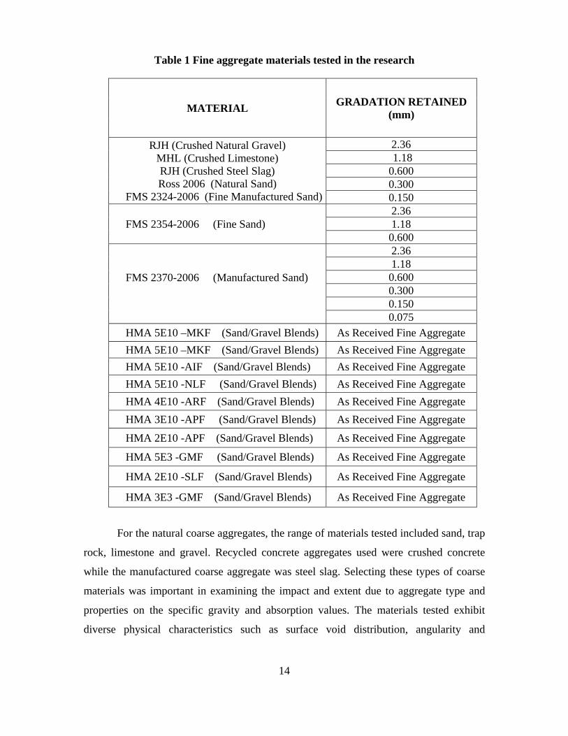
Figure 5. The SSDetect with AVU unit ............................................................................ 23

Figure 6 Internal components of the SSDetect ................................................................. 23

Figure 7 Film Coefficient Curve for the fine sand aggregate ........................................... 25

Figure 8. The set-up of the AASHTO T85 ....................................................................... 27

Figure 10. The Vacuum saturation apparatus used to expel the air in the coarse aggregate

mass and force water into the pores of the aggregates .......................................... 27

Figure 11 AASHTO T-84 against SSDetect Bulk Specific Gravity (dry) ........................ 63

Figure 12 AASHTO T-84 against SSDetect Bulk Specific Gravity (SSD) ...................... 64

Figure 13 AASHTO T-84 against SSDetect Bulk Specific Gravity (Gsa) ....................... 65

Figure 14 AASHTO T-84 against SSDetect Water Absorption (Wa %) .......................... 66

Figure 15 Blended-Calculated against SSDetect Gsb (dry) .............................................. 67

Figure 16 Blended-Calculated against SSDetect Gsb (SSD) ............................................ 68

Figure 17 Blended-Calculated against SSDetect Gsa ....................................................... 69

Figure 18 Blended-Calculated against SSDetect Wa% .................................................... 70

Figure 19 AASHTO T-85 versus 10 Minutes Vacuum Saturation Test for Gsb (Dry) .... 72

Figure 20 AASHTO T-85 against 20 Minutes Vacuum Saturation Test for Gsb (dry) .... 73

Figure 21 AASHTO T-85 against 30 Minutes Vacuum Saturation Test for Gsb (dry) .... 74

Figure 22 AASHTO T-85 against 10 Minutes Vacuum Saturation Test for Gsb (SSD) .. 75



Figure 25 AASHTO T-85 against 10 Minutes Vacuum Saturation Test for Gsa ............. 78



Figure 28 AASHTO T-85 against 10 Minutes Vacuum Saturation Test for Wa% .......... 81

IX



Figure 31 Gsb (Dry): Calculated Value against Single Test Value of 10 Minutes Vacuum

Saturation Test ...................................................................................................... 84

Figure 32 Gsb (Dry): Calculated Value against Single Test Value of 10 Minutes Vacuum

Saturation Test ...................................................................................................... 85

Figure 33 Gsa: Calculated Value against Single Test Value of 10 Minutes Vacuum

Saturation Test ...................................................................................................... 86

Figure 34 Wa%: Calculated Value against Single Test Value of 10 Minutes Vacuum

Saturation Test ...................................................................................................... 87

Figure 35 Gsb (dry) test results over 24, 36, 48 and 72 hours of soaking periods ........... 88

Figure 36 Gsb (SSD) test results over 24, 36, 48 and 72 hours of soaking periods ......... 89

Figure 37 Gsa test results over 24, 36, 48 and 72 hours of soaking periods..................... 90

Figure 38 Wa% test results over 24, 36, 48 and 72 hours of soaking periods .................. 91

X

LIST OF TABLES

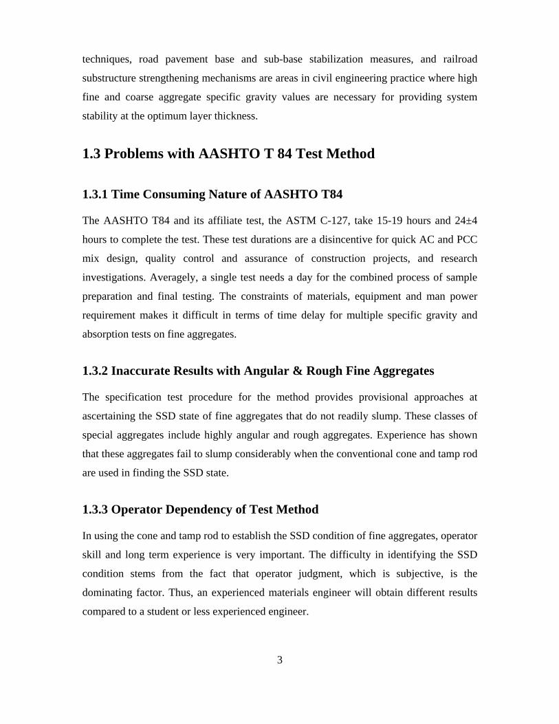
Table 1 Fine aggregate materials tested in the research ................................................... 14

Table 2 Coarse aggregate materials (including highly absorptive aggregates) tested in the

research ................................................................................................................. 15

Table 3 Coarse aggregates tested over extended soaking times ....................................... 16

Table 4 Blended fine aggregates tested (MDOT Designation) ......................................... 28

Table 5 Blended coarse aggregates tested (MDOT Designation) ..................................... 29

Table 6 Spearman correlation coefficients ....................................................................... 31

Table 7 Summary of LSD Means Testing ........................................................................ 33

Table 8 Summary of Tukey Means Testing ...................................................................... 34

Table 9 Statistical Analysis of the AASHTO T 85 versus the Vacuum Saturation Test .. 35

Table 10 Statistical Analysis of the AASHTO T 85 versus the Vacuum Saturation Test 36

Table 11 Gsb (Dry) and Standard Deviation Results for T-84 and SSDetect .................. 53

Table 12 Gsb (SSD) and Standard Deviation Results for T-84 and SSDetect ................. 56

Table 13 Gsa and Standard Deviation Results for T-84 and SSDetect ............................. 58

Table 14 Wa % and Standard Deviation results for T-84 and SSDetectError! Bookmark

not defined.

1

CHAPTER 1 INTRODUCTION

1.1 Background

1.1.1 History of Specific Gravity

The discovery of specific gravity is credited to the famous Greek Mathematician,

Archimedes, dating back to 250 B. C. (Rea 1917). The storyline has it that King Heiro II

of Syracuse contracted Archimedes to evaluate the gold content in a crown made for him

by a metal smith. Archimedes had determined that the quantity of water displaced by his

submerged body in a bath pool was equal in measure to the volume his body occupied in

the bath. Based on this theory, Archimedes was able to determine that a given mass of

silver occupies more volume than an equivalent mass of gold. In his experiment,

Archimedes put the crown molded by King Heiro II’s metal smith in a container full of

water and pure gold in a container of water; he detected that more water spilled from the

container when the molded crown was put in it. This made Archimedes confirm that the

king’s crown was adulterated and not made of pure gold.

1.1.2 Specific Gravity in Civil Engineering Materials

The American Association of State Highway and Transportation Officials (AASHTO)

Standard T-85 defines the specific gravity of an aggregate as the ratio of the density of a

material to the density of distilled water at a stated temperature, the values being

dimensionless. Specific gravity is determined at bulk and apparent conditions. In the

bulk state, denoted Gsb, both the permeable and impermeable voids on the surface on the

aggregate are considered in the volume calculations. Conversely, the apparent specific

gravity (Gsa) calculates the specific gravity excluding the permeable voids of the

aggregate. The absorption potential of an aggregate is the increase in mass of aggregate

due to water penetration into the pores of the particles during a prescribed period of time,

but not including water adhering to the outside surface of the particles, expressed as a

percentage of the dry mass. Gsb (SSD) is used when the fine aggregates are considered to

be wet at the time of use.

2

1.2 Uses & Significance of Specific Gravity and Absorption

Specific gravity and absorption values of fine and coarse aggregates are used in the

following applications:

1.2.1 Volumetric Design of Asphalt and Portland Concrete Cement

(PCC) Pavements

Voids in the mineral aggregate (VMA), voids filled with asphalt (VFA) and the total

voids in mix (VTM) are useful inputs in the volumetric design, mix preparation, and

quality control and assurance of asphalt pavement construction. Water-cement ratio

determinations for PCC mix are vital in ensuring a mix of high structural integrity and

durability. For example, when a highly absorptive aggregate is used in Hot Mix Asphalt

(HMA), more asphalt binder is absorbed. In the case of the PCC mix, mixing water

requirement for better mechanical strength and durability characteristics is increased

when an overly absorptive fine aggregate is used. Less absorptive fine aggregates are

satisfactory for the economical design and construction of most construction works.

1.2.2 Freeze Thaw Issues in Civil Engineering Structure

The freeze thaw potential in concrete mixes for civil infrastructure, AC and PCC

pavements and structures can be evaluated with the knowledge of the specific gravity and

absorption of fine and coarse aggregates. Freeze thaw evaluation is essential for the

elimination of damage due to ingression of water, moisture, snow, and other forms of

precipitation. The cycle freezing and thawing of fine and coarse aggregates result due to

the effect of temperature differential from extreme climatic and environmental changes

A high absorption value of fine aggregates tends to result in moisture-related damage.

1.2.3 Stabilization of Earth Structures and Highway Pavements

Specific gravity differentiation techniques are essential in separating good aggregates

from deleterious (lighter) materials such as degradable materials like wood, leaves and

bones, and non-degradable ones like glass, paper, plastic and rubber. These unwanted

materials reduce the overall specific gravity of coarse aggregates. Erosion control

3

techniques, road pavement base and sub-base stabilization measures, and railroad

substructure strengthening mechanisms are areas in civil engineering practice where high

fine and coarse aggregate specific gravity values are necessary for providing system

stability at the optimum layer thickness.

1.3 Problems with AASHTO T 84 Test Method

1.3.1 Time Consuming Nature of AASHTO T84

The AASHTO T84 and its affiliate test, the ASTM C-127, take 15-19 hours and 24±4

hours to complete the test. These test durations are a disincentive for quick AC and PCC

mix design, quality control and assurance of construction projects, and research

investigations. Averagely, a single test needs a day for the combined process of sample

preparation and final testing. The constraints of materials, equipment and man power

requirement makes it difficult in terms of time delay for multiple specific gravity and

absorption tests on fine aggregates.

1.3.2 Inaccurate Results with Angular & Rough Fine Aggregates

The specification test procedure for the method provides provisional approaches at

ascertaining the SSD state of fine aggregates that do not readily slump. These classes of

special aggregates include highly angular and rough aggregates. Experience has shown

that these aggregates fail to slump considerably when the conventional cone and tamp rod

are used in finding the SSD state.

1.3.3 Operator Dependency of Test Method

In using the cone and tamp rod to establish the SSD condition of fine aggregates, operator

skill and long term experience is very important. The difficulty in identifying the SSD

condition stems from the fact that operator judgment, which is subjective, is the

dominating factor. Thus, an experienced materials engineer will obtain different results

compared to a student or less experienced engineer.

4

1.4 Problems with AASHTO T 85 Test Method

1.4.1 Time Consuming Nature of AASHTO T85

Similar to the AASHTO T84, the AASHTO T85 also takes much testing time to conduct.

The 24±4 hours creates inconveniences for the facilitation of rapid design, construction

quality control and assurance. The construction industry is thus in need of test methods

that will reduce drastically the testing time for specific gravity and absorption

determination of coarse aggregates.

1.4.2 Underestimation of water absorption of porous coarse aggregates

Work at the Michigan Technological University Materials Laboratory has shown that for

some special coarse aggregate types like steel slag and crushed concrete which are highly

porous need extended soaking times to satisfy their full absorptive potential.

5

CHAPTER 2 LITERATURE REVIEW

The development of test methods to determine the specific gravity and absorption of fine

and coarse aggregates dates back to the early days of the 20th century. Researchers and

engineers tried in earnest to identify single and unique methods to serve all concerned

who utilize specific gravity and absorption for practice in civil engineering.

2.1 Fine Aggregate Specific Gravity Test Method Development

Among the early attempts at bulk specific gravity and absorption of fine aggregates was

the work undertaken to find the specific gravity of non-homogenous fine aggregates (Rea

1917). Rea’s approach found the apparent specific gravity by coating sand materials with

kerosene before finding the volume of the sand. The rationale behind coating the fine

aggregates is to prevent the penetration of water into the voids. The ASTM Committee C-

9 on Concrete and Concrete Aggregates revised this early method, of which the details

were carried out in the 1920’s ASTM Proceedings report (ASTM 1920)

Further development of a method to find the specific gravity and absorption of

sand was shown by Pearson. The method involved finding how dampened grains of sand

adhered to the sides of an Erlenmeyer flask (Pearson 1929). Pearson reported that this

proposed method underestimated the true absorption value due to incomplete saturation.

Pearson’s titration method was modified slightly, and accepted by the ASTM for

use as the standard practice for specific gravity and absorption determination (ASTM

1933). The sand was saturated with water and dried back to SSD state based on the

operator’s visual inspection. 500g of the SSD sample was placed in a 1-qt glass jar, and

water added in drops to ascertain whether the material sticks to the sides of the jar. The

SSD state condition of this method according to Pearson was highly subjective and thus

unreliable.

The use of color change in sand SSD determination has proved to be unreliable

and unrepeatable (Chapman 1929) . To further increase the usefulness of the colimetric

method of SSD and specific gravity determination, calcium chloride was used to dry the

sand for some time (Graf and Johnson 1930). The drying process, it was found unduly

removed substantial amounts of water from the SSD sand material.

6

Additional research worth noting is that of Myers in 1935. Myers found the free

moisture in the aggregate using gravimetric, displacement, dilution, colimetric and

electrical-resistance principles. All the four methods were not promising due to the fact

that visual inspection was used in finding the saturated surface dry state of the fine

aggregates during testing (Myers 1935). There have been a number of research advances

towards the modification of how the SSD condition of fine aggregate is determined to

make the test less prone to error. These advances have also aimed at reducing the test

time from about 24 hours to only a few hours.

AASHTO T-84 is currently used to determine the fine aggregate specific gravity

and absorption. The method dates back to 1935 when the kerosene method, ASTM

tentative method, cone method and visual inspection method were evaluated in order to

rank them in terms of which was the most promising. Results from this research showed

that the cone method (AASHTO T 84) was the most favorable among the four test

methods. The T-84 procedure requires approximately 1kg of the fine aggregate be

immersed in water or soaked in at least 6% moisture and allowed to stand undisturbed for

about 15 hours. The rationale behind the soaking of the fine aggregate is to enable the

full water absorption potential of the aggregate pore surfaces to be satisfied before the

specific gravity and absorption are measured in the laboratory. After soaking,

the sample is decanted and spread flat on a nonabsorbent surface exposed to a gentle

current of warm air, constantly stirred until surface dry, and a cone and tamp rod used to

determine its saturated surface-dry state (SSD). The subjectivity of the test in part is

when a tester determines when the fine aggregate just slumps after removal of the cone

and that in fact the slumped sample is uniformly representative of the approximately 1kg

sample.

Attempts at measuring fine aggregate specific gravity based on thermodynamic

principles were initiated by the Arizona Department of Transportation (ADOT)

(Dana and Peters 1974). Dana and Peters had sought to establish the SSD state of fine

aggregates by soaking the sample and placing it in a small rotating drum. As the

aggregates were rotated uniformly, hot air was issued through one end to dry it. An

attached thermocouple, an electronic device that converted the temperature gradient into

an electronic signal, was used to convey data to a digital recorder or sensor. The

attainment of the SSD condition caused a sudden drop in the thermal gradient between

7

the incoming and outgoing air. Their work established that the concept of monitoring the

temperature gradient of incoming and outgoing air or the relative humidity of the

outgoing air had positive results on a wide range of fine aggregates.

Further research on the initiative taken by Dana and Peters added the

measurement of the humidity of the outgoing air to the temperature gradient principle

(Kandhal et al. 2000). The research demonstrated that the humidity of the outgoing air

predicts the SSD condition more accurately than the temperature gradient. A significant

recommendation of this work was the improved automation of the

thermodynamic device to enable the operation to be stopped immediately after the SSD

state is found, and also measuring the final mass of fine aggregate during the process.

The device received enhanced modification by the National Center for Asphalt

Technology (NCAT) but the repeatability and reproducibility of test results was poor.

In other fine aggregate research developments, the idea of establishing the SSD

condition of fine aggregates by examining their flow under gravity off a tilted masonry

trowel has been exploited (Krugler et al. 1992). This approach defines the SSD condition

to be the state when the aggregates are capable of flowing off freely as discrete individual

particles. A second proposed method by Krugler involved placing the fine aggregate

samples adjacent to oven-dry ones; and the SSD condition determined as the point where

the test materials have the same color as the oven-dry aggregate. Another technique

Krugler considered was based upon sliding test samples along the bottom of a tilted pan.

When the test sample failed to stick to the bottom and flowed freely, the SSD state was

judged to have been reached.

The use of water-soluble glue to detect whether fines aggregates have achieved

SSD or not was also developed, and compared to earlier methods at specific gravity

measurement (Krugler et al. 1992). Krugler et al. employed a strip of packaging tape

(Supreme Super standard gummed paper tape, 5.08 cm medium duty), attached it to a

small block of wood and placed the wood with glue on the fine aggregate material. The

proposition was that if for two trials not more than one test-sample particle adheres to the

tape, the sample was judged to have attained the SSD condition.

Fine aggregates have been known to undergo color transformations with the

presence of water on the particle’s surfaces. This colimetric idea of establishing the SSD

condition of fine aggregates has been studied and investigated by some researchers

8

(Lee and Kandhal 1970). The process basically uses a special chemical dye to achieve the

same SSD requirements of the AASHTO T-84 procedure. The fine aggregate is first

soaked in water containing the dye. When removed from the water, the aggregate which

has now taken the color of the dye begins to dry. SSD is said to be reached when the

aggregate changes from this color status after receiving dry current from a fan. Lee and

Kandhal noted that the dyes never showed well on dark-colored aggregates, exhibited

non-uniform mixing when the fine aggregates were being dried and the color change was

highly subjective. These notable and problematic observations made this proposition

impracticable and difficult.

Some important successes in specific gravity research worth mentioning are

Saxer’s absorption curve procedure (Saxer 1956), Hughes and Bahramain’s saturated air-

drying method (Hughes 1967) and Martin’s wet and dry bulb temperature method

(Martin 1950). These test methods required a high level of expertise to perform and to

improve their practicability, extensive modifications were suggested.

Quite recently, automated equipment such as the SSDetect, AggPlus and the

Langley system have been developed by material testing engineers to address the

aforementioned limitations of AASHTO T84. For example, the SSDetect, which is more

scientific in nature, has been known to have statistically similar results with AASHTO

T84 according to research conducted on Oklahoma fine aggregates (Cross 2006). Cross et

al. also demonstrated that the new SSDetect could have better repeatability than the

traditional fine aggregate specific gravity and has great potential in replacing AASHTO

T84. Cross et al. reported that this electronic innovation had great potential in specific

gravity measurement since the vacuum sealed results were comparable to that of the

AASHTO T84.

Another significant scientific input towards improvement in specific gravity

determination is the use of the vacuum sealing approach – a single test method (Hall

2002). The method measures specific gravity by using electronic vacuum sealing

procedure to expel fine aggregates packed in standard polythene bags. Hall observed also

that tests of aggregate blends do not appear to be sensitive to nominal maximum

aggregate size, gradation nor mineralogy.

At Michigan Technological (Tech) University, researchers investigated the

applicability of the automated helium pycnometer in fine aggregate specific gravity

9

analysis in geotechnical engineering (Vitton et al. 1999). Current specific gravity test

methods require soaking for close to 24 hours to satisfy most of the absorption potential.

However, it is recognized that for some highly absorptive aggregates, not all of the

effective pore space may be saturated after 24 hours. Helium gas, on the other hand, can

more easily absorb into a material’s effective pore space. The helium pycnometer uses

the ideal gas law, PV=nRT, to determine the volume of a material based on pressure

measurements of helium gas. By knowing the dry mass of a soil, the specific gravity of

the aggregate can be determined.

Michigan Tech researchers explored another alternative (Vitton et al. 1999) -- the

automated envelope density analyzer. This device determines the bulk volume or

envelope volume of a sample by measuring the volume of a fine-grained material in a

cylinder, and then again measuring the volume of the fine-grained material plus the

sample. By finding the difference in volume between the two measurements, the bulk

volume of the sample can be calculated and the bulk specific gravity determined. The

findings concluded that the helium pycnometer can be used to automate the testing of

aggregate to determine apparent specific gravity. A combination of the helium

pycnometer and the envelope density analyzer can be used to calculate the absorption and

bulk specific gravity (SSD).

In Michigan Technological University, You et al. (2008) conducted research on

the fine aggregate specific gravity by comparing the SSDetect and AASHTO T84. It was

found that the SSDetect and AASHTO T84 had very good correlation in specific gravity.

This paper is based upon the existing work and expanded tested materials.

There are some other methods such as a gamma-ray method (Core Reader), Paraffin-

Coated test, and other methods used in HMA and Portland cement concrete (PCC)

materials testing. The CoreLok (vacuum sealing) method has been evaluated further by a

number of state transportation agencies and many universities (Prowell and Baker 2004).

Table 2 is a summary of some of the research work conducted for fine aggregate specific

gravity testing.

10

2.2 Coarse Aggregate Specific Gravity Test Method

Development

The challenges that result from the AASHTO T85 (ASTM C-127) test method for coarse

aggregate specific gravity and absorption has prompted many researchers to explore how

best this test approach can be improved.

Washburn and Bunting (Washburn and Bunting 1922) employed a gas expansion method

based on Boyle’s law to determine porosity of coarse aggregates. In this research,

isolated voids were counted as solids, and thus the method measured effective porosity if

the sample is not powdered. Knowledge of the effective porosity was critical in finding

the specific gravity and water absorption percent of the coarse aggregates.

In 1959, Dolch (Dolch 1959) further expanded on the knowledge of effective

porosity by conducting tests on limestone aggregates, measuring the parameter with the

McLeod gauge porosity developed by Washburn and Bunting (Washburn and Bunting

1922). Dolch’s research objective was to evaluate how the physical characteristics of

aggregates impact on their specific gravity and absorption determination. The method

gives a value for the effective void volume by causing the head to be lowered on a dry

sample while it is immersed in mercury. The air in voids expands and leaves the sample

and is then measured volumetrically at atmospheric pressure. The porosity was then

obtained after the bulk volume of the sample was determined by the use of shaped pieces.

One of the most effective and frequently used methods of determining the specific

surface of a solid was the sorption method (Brunauer (1938)). The specific surfaces were

obtained from sorption isotherms. The sorption absorption method had also been used

indirectly to obtain a curve for pore size distribution. Other methods for determining pore

size and specific surface are small angle – ray scattering, heat of immersion, rate of

dissolution, ionic adsorption, and radioactive and electrical methods.

During the early 1970’s, the most frequently used method of absorption

determination was the injection of mercury into the pore system (Ritter and Erich July

1948). The pressed mercury was used in finding the pore size distribution of aggregates.

The model was based on the assumption that the pores existed as a system of circular

capillaries. Washburn established that the relationship between the applied pressure, p;

11

radius of the pore, r; surface tension of mercury, σ; contact angle between the mercury

and the solid coarse aggregate, θ; is given as:

p = - 2 σ cos θ. [1]

Further development was based upon Washburn and Bunting's concept for

practical use, and thus an apparatus was developed for measuring the penetration of

mercury into aggregate pores (Drake 1945). The apparatus is generally referred to as a

mercury porosimeter. Subsequently, Drake (Drake 1945) utilized a high pressure mercury

porosimeter. The mercury penetration method has been used over a range of pore sizes in

research work and has been applied successfully to PCC aggregates (Hiltrop 1960).

During the first year of a Highway Research Project HR-142 (Lee and Kandhal

1970), a special study was conducted to develop new, simple, and more reproducible

method to determine the bulk specific gravity or the saturated surface-dry condition for

granular materials. As a result, a new chemical indicator method was developed to

determine the saturated surface-dry condition, and a glass mercury pycnometer was

designed to determine the bulk specific gravity of large aggregates.

Vitton et al. (Vitton et al. 1999) investigated the applicability of the automated

helium pycnometer in aggregate specific gravity analysis in geotechnical engineering.

The research targeted how to best measure the specific gravity of highly absorptive

coarse aggregates. This was necessitated by the discovery that the conventional

24±4hours failed to satisfy the full absorption potential of highly absorptive aggregates.

Helium gas, on the other hand, can more easily absorb into a material’s effective pore

space. A helium pycnometer uses the ideal gas law, PV=nRT, to determine the volume of

a material based on pressure measurements of helium gas. By knowing the dry mass of

the aggregate, the specific gravity of the aggregate can be determined. Another

alternative Vitton et al. (Vitton et al. 1999) explored was the use of the automated

envelope density analyzer. This device determines the bulk volume or envelope volume

of a sample by measuring the volume of a fine-grained material in a cylinder, and then

again measuring the volume of the fine-grained material plus the sample. By finding the

difference in volume between the two measurements, the bulk volume of the sample can

be calculated and the bulk specific gravity determined. The findings concluded that the

12

helium pycnometer can be used to automate the testing of coarse aggregates to determine

apparent specific gravity while the envelope density analyzer is applicable for specific

gravity measurement of coarse aggregates. A combination of the helium pycnometer and

the envelope density analyzer can be used to calculate the absorption, and bulk specific

gravity (SSD).

Hall (Hall 2002) performed research work on improving the existing AASHTO T

85 method of specific gravity and absorption testing of coarse aggregates. This work

concentrated basically on the evaluation of the use of a single test – vacuum sealing

approach - to determine specific gravity and absorption of coarse aggregate blends. The

process involves using the vacuum sealing device to suck all entrapped air within the dry

coarse aggregate which has been placed in a standard plastic bag. The vacuum sealing

method eliminates the traditional long soaking periods. Hall compared his results with

mathematical combinations of specific gravities from the individual tests. The research

revealed statistically similar results. Hall added that the tests of aggregate blends do not

appear to be sensitive to nominal maximum aggregate size, gradation or mineralogy.

13

CHAPTER 3 MATERIALS TESTED

3.1 Fine Aggregate Materials

The aggregates used in the research work were typical of those found in the state of

Michigan. Sand and gravel are two of the most important sources of fine aggregates

commonly found throughout the northern part of the United States due to glacial deposits

and occur in other parts of the United States from old lake or river beds.

The research considered a range of fine aggregate source materials with varying

gradations to determine if their specific gravity and absorption values measured by the

SSDetect were comparable to AASHTO T 84. Fine materials that have been used in this

study are listed in Table 1. The four source materials shown with the various sieve sizes

were tested for each sieve fraction as indicated, while the last 10 source materials in the

table were tested as “as received” gradation ranging in sieve size from the 4.75 to the

0.075mm sieve. The Ross 2006, FMS 2354-2006, FMS 2370-2006 and FMS 2324-2006

fine aggregates had 44, 58, 51 and 50% carbonate minerals respectively. Siliceous and

other minerals contained in the Ross, 2354, 2370 and 2324 were 56, 42, 49 and 50 %,

respectively. In addition to the blended ‘as received’ fine aggregate blend, a number of

the aggregates were blended to attain Michigan Department of Transportation (MDOT)

specifications, namely gradations. These materials were tested with the SSDetect device.

The MDOT blended gradations that were used in this analysis are shown in Table 1.

3.2 Coarse Aggregate Materials

The materials that were considered for this research were typical of natural, recycled and

manufactured coarse aggregates currently used in the construction industry in Michigan.

Michigan aggregates represent those that are ideal for both the cold (winter) and hot

(summer) climates of the United States. These aggregates thus have strength and material

properties that are similar to those used in other parts of the United States.

14

Table 1 Fine aggregate materials tested in the research

MATERIAL GRADATION RETAINED (mm)

RJH (Crushed Natural Gravel) MHL (Crushed Limestone) RJH (Crushed Steel Slag) Ross 2006 (Natural Sand)

FMS 2324-2006 (Fine Manufactured Sand)

2.36 1.18 0.600 0.300 0.150

FMS 2354-2006 (Fine Sand) 2.36 1.18 0.600

FMS 2370-2006 (Manufactured Sand)

2.36 1.18 0.600 0.300 0.150 0.075

HMA 5E10 –MKF (Sand/Gravel Blends) As Received Fine Aggregate HMA 5E10 –MKF (Sand/Gravel Blends) As Received Fine Aggregate HMA 5E10 -AIF (Sand/Gravel Blends) As Received Fine Aggregate HMA 5E10 -NLF (Sand/Gravel Blends) As Received Fine Aggregate HMA 4E10 -ARF (Sand/Gravel Blends) As Received Fine Aggregate HMA 3E10 -APF (Sand/Gravel Blends) As Received Fine Aggregate

HMA 2E10 -APF (Sand/Gravel Blends) As Received Fine Aggregate

HMA 5E3 -GMF (Sand/Gravel Blends) As Received Fine Aggregate

HMA 2E10 -SLF (Sand/Gravel Blends) As Received Fine Aggregate

HMA 3E3 -GMF (Sand/Gravel Blends) As Received Fine Aggregate

For the natural coarse aggregates, the range of materials tested included sand, trap

rock, limestone and gravel. Recycled concrete aggregates used were crushed concrete

while the manufactured coarse aggregate was steel slag. Selecting these types of coarse

materials was important in examining the impact and extent due to aggregate type and

properties on the specific gravity and absorption values. The materials tested exhibit

diverse physical characteristics such as surface void distribution, angularity and

15

sphericity. The tested materials, with their respective gradations for the research project

are given in Table 2.

Table 2 Coarse aggregate materials (including highly absorptive aggregates) tested

in the research

Coarse Aggregate Material

Tested Sieve Sizes (Retained)

ROSS ( Sand) # 4 Red Crushed Stone # 4

Trap Rock 3/8''

Steel Slag (highly absorptive aggregates)

# 4 3/8'' 1/2'' 3/4''

Crushed (Recycled) Concrete (highly absorptive aggregates)

# 4 3/8'' 1/2'' 3/4''

Limestone

# 4 3/8'' 1/2'' 3/4'' 1''

River Gravel

# 4 3/8'' 1/2'' 3/4'' 1''

In addition to the 24 hours soaking times required for the AASHTO T-85, the

specific gravities and water absorption percent of steel slag extended soaking times of 36,

48 and 72 hours were investigated. The tested materials at their various gradations are

shown in Table 3. Table 3 shows the different types of absorptive or highly porous coarse

aggregates tested in addition to the steel slag. Crushed or recycled concrete, gravel and

limestone were evaluated for their absorptive capacity over the extended soaking times.

16

Table 3 Coarse aggregates tested over extended soaking times

Material Gradation retained

Slag (highly absorptive aggregates)

#4

Crushed concrete (highly absorptive

aggregates) 1/2"

Gravel 3/4"

Limestone 1/2"

17

CHAPTER 4 RESEARCH METHODOLOGY

4.1 The SSDetect Automated Approach

The research methodology involved the exploration of two methods that could serve as

better alternatives for the determination of the specific gravity and absorption of fine and

coarse aggregates. For fine aggregates, the Automated SSDetect is selected as a

potentially good substitute for the conventional AASHTO T 84. The SSDetect was

evaluated to determine its potential to test the fine aggregates in less than 60 minutes

while providing more repeatable and accurate results. Additionally, the equipment could

eliminate the element of operator dependency which was associated with the AASHTO T

84. The SSDetect basically operates on the laws of reflection and scattering of light rays

to determine when fine aggregates have reached their SSD state. The hypothesis is that

unlike the AASHTO T 84, the SSDetect could eliminate the subjectivity in finding the

SSD condition of the fine aggregates when testing for their specific gravity and

absorption. Figure 1 indicates the flow chart diagram for the exploring the difference

between the SSDetect and the AASHTO T 84.

4.2 The Vacuum Saturation Approach

The Vacuum Saturation Approach is the proposed method that could serve as a viable

alternative for the AASHTO T 85. The approach involves employing the use of the rice

vacuum saturation method to replace the existing 24 ±4 hours soaking procedure which is

characteristic of AASHTO T 85. The method can be thought of as an incorporation of the

standard method for finding the theoretical maximum density, Gmm, of asphalt paving

mixtures into finding the specific gravity and absorption of the coarse aggregates. Rice

in 1952 developed this asphalt mixture testing approach to determine its void content

using pressure. The first part of the test procedure is the vacuum saturation process, after

which the coarse aggregate SSD state is determined using a dry absorbent cloth which is

specified in AASHTO T 85. Vacuum saturating the aggregates were conducted at three

selected time periods – 10, 20 and 30 minutes. The choice of these time durations was to

evaluate which of the three produces the most statistically similar specific gravity and

absorption values with AASHTO T 85. In terms of the vacuum pressure, a 30 ± 2mm (4.0

± 0.5kPa) was chosen to remove all the entrapped air within the coarse aggregate mass

and replace any air voids within the effective pores of the aggregates with water.

18

Figure 1. Flow chart indicating the processes carried out for the AASHTO T 84

against the SSDetect

FINE AGGREGATE MATERIAL (- 4.75mm Gradation)

SSDETECT TEST METHOD AASHTO T-84 TEST METHOD

15-19 HOURS SOAKING OF FINE AGGREGATE

FINE AGGREGATE FILM COEFFICIENT DETERMINATION

DECANTATION AND SSD STATE DETERMINATION

SSD STATE DETERMINATION USING INFRA-RED SCATTERING

OVEN DRY WEIGHT OF FINE AGGREGATE

SSDETECT BOWL + AGGREGATE WEIGHT MEASUREMENTS

SPECIFIC GRAVITY AND ABSORPTION CALCULATIONS

19

4.3 The Statistical Analysis of Results

Three replicates were tested for each of the fine and coarse aggregate materials. The

sources sampled and investigated were natural, manufactured and recycled aggregates.

For both the fine and coarse aggregates, three trial tests were conducted per individual

sieve size and blended gradation, and the results averaged to represent the specific gravity

and absorption values.

Spearman correlation coefficient, least square difference, Tukey test and paired t-

Test for difference in mean values were utilized in analyzing the results of the AASHTO

T 84 and SSDetect test methods. In evaluating the difference between the AASHTO T 85

and the Modified Rice Test Method, the paired t-Test for mean difference and the

confidence interval for mean values were used.

20

CHAPTER 5 THE AUTOMATED SSDETECT

5.1 Standard AASHTO T-84 Test Method

The fine aggregates were initially tested according to AASHTO T 84, Standard Test

Method of Test for Specific Gravity and Absorption of Fine Aggregate. About 1000g of

the fine aggregate, sampled using the AASHTO T 248 Test Procedure, Reducing Field

Samples of Aggregates to Testing Sizes, was dried at a constant temperature of 110 ± 5°C.

Upon cooling to handling temperature, the material was immersed in 6-percent moisture

and allowed to stand overnight for 15 hours. The water was decanted and spread on a flat

non-absorbent surface. With the aid of moving current from a hair drier, the fine

aggregates were continuously dried and stirred. Within intervals, portions of the partially

dried fine aggregates were put in the frustum cone, and made to heap above the top of the

mold. 25 light blows of the tamping rod are applied to the fine aggregate, and into the

mold. The slight slump of the tested aggregates gave an indication of the SSD state. The

frustum cone and tamping rod used is shown in figure 2. The mathematical calculations

of the specific gravities were conducted according to the formulae in the Appendix of the

AASHTO T84 test procedure.

Figure 2. The AASHTO T84 set-up

5.2 SSDetect Test Method

The SSDetect device works on the basic principle of the laws of reflection. Objects can

be seen by their characteristic nature of reflecting light rays that fall on them. The

reflected light rays conform to the scientific law of reflection, which in simpler terms

proves that the angle of reflection is equal and opposite to that of the angle of incidence.

The law of reflection is represented pictorially in figure 3.

Some objects however exhibit scattering of light rays – a phenomenon which

occurs when light rays are reflected at a number of angles after the incident rays fall on

uneven or granular surfaces. Fine aggregates, like most materials, obey the law of

reflection when viewed on the microscopic level but since the irregularities on its surface

are larger than the wavelength of light, the light is reflected in many directions. This

phenomenon is indicated in figure 4. The SSDetect operates on this principle to ascertain

the SSD state of the fine aggregates when thin films of moisture are coated on the

particles. The surface moisture causes diffusive reflection of the rays which are then

picked up by the laser system in the SSDetect unit. The new SSDetect basically involves

a 2- step procedure: determination of the film coefficient and infra-red detection of the

SSD condition of the fine aggregate sample.

21

Normal Angle of incidence (i°) Angle of reflection (r°)

Law of Reflection: iº = rº

Figure 3. The Law of reflection of light on an even surface

Incident rays

Scattered rays

Figure 4. Scattering of light rays on an uneven surface (fine aggregate

22

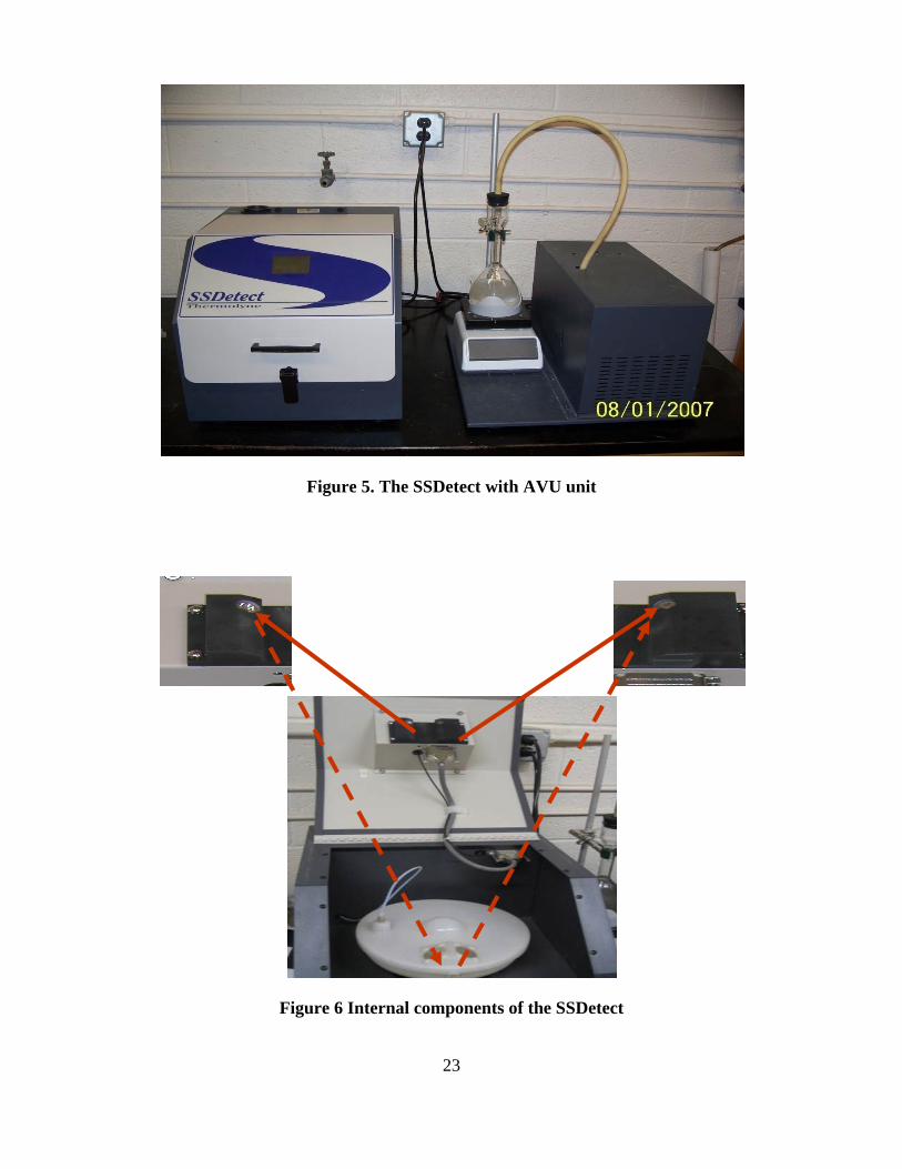
Figure 5. The SSDetect with AVU unit

Figure 6 Internal components of the SSDetect

23

24

5.2.1 Film Coefficient Determination

The film coefficient or “Baseline” test was conducted to determine the minimum amount

of water needed to form an effective film coating on a unit fine aggregate particle. 500g

of the fine aggregate and 250ml of water was put into a pycnometer, and water filled to

the calibration line before the final total mass was found. After vacuum agitating the

pycnometer with contents using the Automated Vacuum Unit (AVU), water was refilled

back to the calibration line and total mass of pycnometer plus contents determined. This

film coefficient value, which is empirical and increases as aggregate size increases, was

calculated by the following formula:

Fc = 52 + 4x – (0.11x2) [1]

Where:

Fc is the film coefficient value and;

x is the difference between the initial and final mass of the pycnometer and its

contents.

A plot of the film coefficient of a characteristic film coefficient curve for the fine

sand aggregate material used in this research is shown is figure 7.

5.2.2 Infra-Red Detection of SSD Condition of Fine Aggregates

A second 500g of the fine aggregate was put into the special SSDetect bowl and the film

coefficient value entered into the system input screen. The special SSDetect bowl has

been designed specifically, in terms of dimensions and style, to ensure the complete

orbital mixing of the fine aggregate material before it attains the SSD state. Once

initiated, the SSDetect unit injected water through a nozzle mounted on the lid of the test

bowl into the flow of the material. The SSDetect mixes the fine aggregate inside the bowl

by using an orbital motion. Through capillary action and hysteresis, the water is absorbed

into the pores of the aggregate. The forces of capillary and hysteresis act very strongly to

pull water into the aggregate pores quickly. Upon satisfying the optimum water potential

of the fine aggregate pores, the water begins to gather on the surface of the aggregate.

Wetting Curve ( Fine Sand )

50

60

70

80

90

100

0 2 4 6 8 10 12

Mass of Water to Fill Voids (g)

Film

Coe

ffici

ent V

alue

Figure 7 Film Coefficient Curve for the fine sand aggregate

As the process continued, infra-red rays were transmitted through a transparent

lens on the top of the bowl unto the fine aggregate surface. The reflected infra-red rays

then indicated the SSD state of the fine aggregate. The test duration is approximately 2

hours. After the test, the mass of the SSD sample was determined, and the difference

between the 500g fine aggregate and final SSD mass calculated as the water absorbed

during the SSDetect test.

5.2.3 SSDetect Mathematical Relationships

Finding the specific gravity and percent absorption with the SSDetect of the fine

aggregate involves the following mathematical computations:

Gsb (Dry) = A/ (A+B-C+D) [2]

Gsb (SSD) = (A+D)/(A+B-C+D) [3]

Gsa = E/(E+B-C) [4]

Wa% = (D/A) x 100 [5]

Where A is the dry sample mass in SSDetect bowl in grams; B is the mass of volumetric

flask filled with water in grams; C is the final mass in grams of flask with contents in film

coefficient determination; D is the water absorbed by the 500g fine aggregate in the

SSDetect bowl; and E is the mass in grams of dry aggregate in film coefficient

determination test. 25

26

CHAPTER 6 THE VACUUM SATURATION

METHOD

6.1 Standard AASHTO T-85 Test Method

Coarse aggregate samples are immersed in water for an approximate 24±4 hours. This

specification was from ASTM C-127 – 04, after which the AASHTO T85 was followed.

The soaked aggregates were then removed from the soaking chamber, and rolled in a dry

non-absorbent cloth to trap all the available moisture on the surface of the coarse

aggregates. The relevant weights that were taken for the specific gravity and absorption

include the SSD weight (submerged and in air condition) and the oven (dry) weights.

6.2 Vacuum Saturation Approach

The proposed research methodology involves employing the use of the rice vacuum

saturation method to replace the existing 24 ± 4 h soaking procedure which is

characteristic of AASHTO T 180. The method can be thought of as an incorporation of

the standard method for finding the theoretical maximum density, Gmm, of asphalt

paving mixtures into finding the specific gravity and absorption of the coarse aggregates.

Rice [12] in 1952 developed this asphalt mixture testing approach to determine its void

content using pressure. The first part of the test procedure is the vacuum saturation

process, after which the coarse aggregate SSD state is determined using a dry absorbent

cloth which is specified in AASHTO T 85. Vacuum saturating the aggregates were

conducted at three selected time periods – 10, 20 and 30 min. The choice of these time

durations was to evaluate which of the three produces the most statistically similar

specific gravity and absorption values with AASHTO T 85. In terms of the vacuum

pressure, a 30 ± 2 mm (4.0 ± 0.5 kPa) Hg was chosen to remove all the entrapped air

within the coarse aggregate mass and replace any air voids within the effective pores of

the aggregates with water. Three replicates were tested for each coarse aggregate source.

The sources studied were natural, manufactured and recycled aggregates. Averages of the

calculated values from the three replicate tests were used as the representative specific

gravity and absorption values.

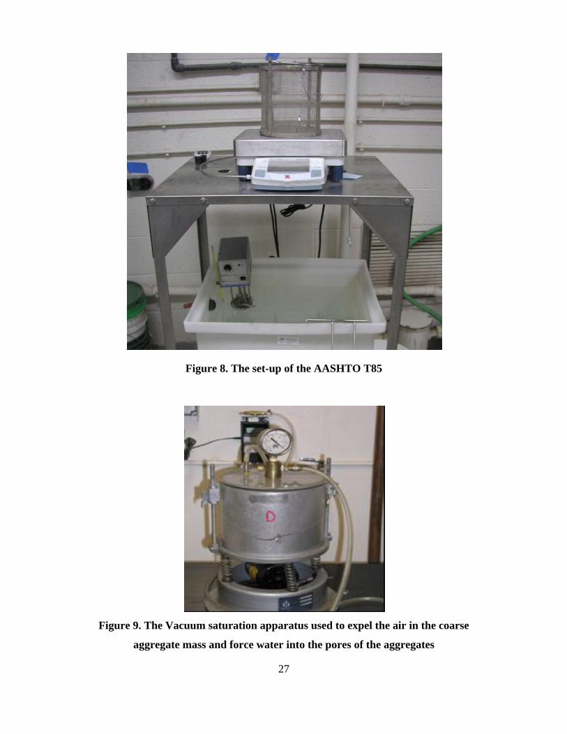
Figure 8. The set-up of the AASHTO T85

Figure 9. The Vacuum saturation apparatus used to expel the air in the coarse

aggregate mass and force water into the pores of the aggregates

27

28

CHAPTER 7 TESTING BLENDED FINE AND

COARSE AGGREGATES

7.1 SSDetect for Blended Fine Aggregates

In the standard AASHTO T-84 specific gravity and absorption testing, blended fine

aggregates are tested in two ways: testing the blended fine aggregate together or using the

proportionate formula to find a calculated blended specific gravity and absorption value.

The calculated specific gravity is obtained using the formula below:

Gsbc = 1/ [(Pb1/Gsb1) + (Pb2/Gsb2) + (Pb3/Gsb3) + ...] (6)

Where:

Gsbc is the specific gravities at either dry, SSD, or apparent conditions; Gsb1, Gsb2, and

Gsb3 are the specific gravities of the first, second, and third individual fine aggregates

used in the total blend; and Pb1, Pb2, and Pb3 are the percentage contributions of the

first, second, and third individual fine aggregates used in the total blend.

To determine whether the calculated blend values were comparable to the

SSDetect values for the blend, the prepared MDOT blends were tested with the SSDetect

and their individual gradation values used to obtain the calculated values. Table 4 gives

the fine aggregate MDOT blends tested with the SSDetect.

Table 4 Blended fine aggregates tested (MDOT Designation)

MATERIAL MDOT RATING

TOTAL PERCENT PASSING

# 4 # 8 # 16 # 30 # 50 # 100

Natural Sand, Fine and Manufactured Sand, Limestone,

Gravel and Slag Fines

2 NS 100 65 35 20 10 0

2 SS 100 80 50 25 15 0

2 MS 100 95 0 0 30 0

29

7.2 Vacuum Saturation Method for Blended Coarse

Aggregates

In parallel with the work done in blending the fine aggregate and testing them as such,

the coarse aggregates were blended according to MDOT blend specifications. The coarse

aggregate blends, with the respective contributions of the individual sieves, are shown in

Table 5.

Table 5 Blended coarse aggregates tested (MDOT Designation)

MATERIAL MDOT RATING

TOTAL PERCENT PASSING

1" 3/4" 1/2" 3/8" #4 #8

Limestone

Steel Slag

Crushed Concrete

25A 100 100 96 60 30 0

26A 100 100 98 60 25 0

29A 100 100 100 90 10 0

6AAA 100 85 30 0 0 0

6AA 95 0 30 0 0 0

30

CHAPTER 8 RESULTS AND ANALYSIS

8.1 AASHTO T84 versus SSDetect

8.1.1 Individual Gradations and As Received Fine Aggregates

The results of the source aggregates (individual gradations) and the as received fine

aggregates are summarized in this section separately. Table 1, 2, 3, and 4 in Appendix A

section gives detailed results of the all the Gsb (dry), Gsb (SSD), Gsa and Wa % tests for

both AASHTO T-84 and SSDetect, and their standard deviations values.

8.1.2 Bulk Specific Gravity (Dry)

The plot of bulk specific gravity (dry) relationship between the AASHTO T-84 and

SSDetect showed a good relationship with an R2 of 0.925 and is shown in Figure 1 of

Appendix B. A large percentage of the fine aggregates tested, 97.7% (42 of 44), satisfied

the AASHTO T-84 acceptable standard specification range (single-operator precision) of

0.032 for any similar given fine aggregate material. The paired t-test for mean Gsb (dry)

analysis at the 95 % significance level showed that there was no significant difference

between the two methods. The confidence interval for difference in mean Gsb (dry) was

found to be (-0.0108, 0.0008) about the mean values.

8.1.3 Bulk Specific Gravity (SSD)

The coefficient of correlation for the Gsb (SSD) was good with an R2 of 0.925 and is

shown in Figure 2 of Appendix B. For the Gsb (SSD), 97.7% of the results satisfied the

acceptable standard specification range (single-operator precision) of 0.027 representing

42 out of the 44 results. The results also showed no statistical difference at the 95% level

of significance with a confidence range of between -0.0039 and 0.0059 about the mean

values.

8.1.4 Apparent Specific Gravity (Gsa)

Approximately two thirds, 28 out of the 43 results, satisfied the AASHTO T-84 range

(single-operator precision) of 0.027 with an R2 coefficient of 0.721 and is summarized in

Figure 3 of Appendix B. With a mean difference range of between 0.0056 and 0.0264,

the paired t-test showed a significant difference between the measurements of the two

methods at a 95% level of significance.

8.1.5 Water Absorption (Wa %)

The coefficient of determination was poor with an R2 of 0.235 and is shown in Figure 4

of Appendix B. 14 of the 44 results (97.7%) satisfied the acceptable standard

specification range (single-operator precision) of 0.31. The results also showed statistical

difference at the 95% level of significance with a confidence range of between 0.634 and

0.310 about the mean values.

8.2 Spearman Correlation Coefficients

Table 6 summarizes the correlation coefficients between AASHTO T84 and the SSDetect

methods for determining the Gsb (dry), Gsb (SSD), Gsa and Wa %. The correlation

coefficients are high for Gsb (dry), Gsb (SSD) and Gsa for the two different methods;

with all of the values greater than 0.80. However, the correlation coefficient between the

two methods is rather low, 0.405, for the Wa %.

Table 6 Spearman correlation coefficients

Gsa

Wa %

SSDETECT

TEST METHOD / RESULT

0.801

0.405

Gsb (dry) 0.894

0.899Gsb (SSD)

AASHTO T84

Gsb (dry) Gsb (SSD) Gsa Wa %

31

32

8.3 Least Square Difference & Tukey Test

Statistical means testing was conducted to examine if statistical differences exist between

the two methods. The three types of specific gravities and water absorption for the sieve

sizes were analyzed using means tests. This consisted of determining the difference

between the levels of each factor and calculating a 95% confidence interval. The

confidence intervals and the significance of the differences were calculated using two

methods: Least Squares Difference (LSD) and Tukey. The LSD method controls the

Type I comparisonwise error rate while the Tukey method controls the Type I

experimentwise error rate and results in the LSD method being less conservative in the

means testing than the Tukey Method. The outcome of these mean tests is summarized in

Table 7 and 8.

120 mean comparisons were done for all sieve size combinations using the LSD

and Tukey methods. 53 mean differences were identified for the LSD method as

identified in Table 7 with “Yes” whereas 36 mean differences were identified for the

Tukey method as shown in Table 8. Both methods of determining the three different

specific gravities using both types of means comparisons show that the specific gravity

values for the sieve sizes (#8, #16, #30, #50, and #100) are different than the #200 sieve

size.

The results of the means testing for the other sieve size comparisons for the

specific gravities were not consistent as some means were different and in other instances

the means were not different. These results lead to the belief that the SSDetect better

determines the three specific gravities for the #8, #16, #30, #50, and #100) sieve sizes

than for the #200 sieve. This could be due to the fact that the SSDetect laser beam is not

effective in finding the SSD state of a closely-packed #200 particles. The closeness of the

particles makes it impossible for the infra-red rays to locate other SSD state particles

aside the ones at the surface. There is thus, non-uniformity in SSD determination when

the #200 is tested.

The outcomes of the means comparisons for the water absorption for both

AASHTO T84 and the SSDetect were inconsistent.

Table 7 Summary of LSD Means Testing

Sieve Comparison

AASHTO T-84 SSDetect

Gsb, dry Gsb, ssd Gsa Wa Gsb, dry Gsb, ssd Gsa Wa

#8 vs. #16 Yes Yes No No Yes Yes No Yes

#8 vs. #30 No No Yes No Yes No No Yes

#8 vs. #50 No Yes Yes No Yes No No Yes

#8 vs. #100 No Yes Yes No Yes No No Yes

#8 vs. #200 Yes Yes Yes No Yes Yes Yes No

#16 vs. #30 No No No Yes No No No No

#16 vs. #50 No No Yes Yes No No No No

#16 vs. #100 No No Yes Yes No Yes Yes No


#30 vs. #50 No No No No No No No No






33

Table 8 Summary of Tukey Means Testing

Sieve

Comparison AASHTO T-84 SSDetect

Gsb, dry Gsb, ssd Gsa Wa Gsb, dry Gsb, ssd Gsa Wa

#8 vs. #16 No No No No Yes Yes No No


#8 vs. #50 No No Yes No Yes No No No

#8 vs. #100 No No Yes No No No No No



#16 vs. #50 No No No Yes No No No No









34

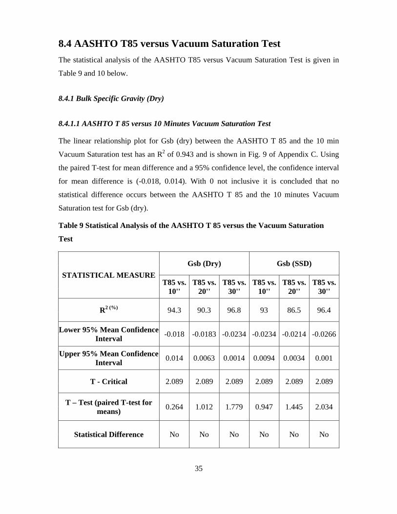
35

8.4 AASHTO T85 versus Vacuum Saturation Test

The statistical analysis of the AASHTO T85 versus Vacuum Saturation Test is given in

Table 9 and 10 below.


8.4.1.1 AASHTO T 85 versus 10 Minutes Vacuum Saturation Test

The linear relationship plot for Gsb (dry) between the AASHTO T 85 and the 10 min

Vacuum Saturation test has an R2 of 0.943 and is shown in Fig. 9 of Appendix C. Using

the paired T-test for mean difference and a 95% confidence level, the confidence interval

for mean difference is (-0.018, 0.014). With 0 not inclusive it is concluded that no

statistical difference occurs between the AASHTO T 85 and the 10 minutes Vacuum

Saturation test for Gsb (dry).

Table 9 Statistical Analysis of the AASHTO T 85 versus the Vacuum Saturation

Test

STATISTICAL MEASURE Gsb (Dry) Gsb (SSD)

T85 vs. 10''

T85 vs. 20''

T85 vs. 30''

T85 vs. 10''

T85 vs. 20''

T85 vs. 30''

R2 (%) 94.3 90.3 96.8 93 86.5 96.4

Lower 95% Mean Confidence Interval -0.018 -0.0183 -0.0234 -0.0234 -0.0214 -0.0266

Upper 95% Mean Confidence Interval 0.014 0.0063 0.0014 0.0094 0.0034 0.001

T - Critical 2.089 2.089 2.089 2.089 2.089 2.089

T – Test (paired T-test for means) 0.264 1.012 1.779 0.947 1.445 2.034

Statistical Difference No No No No No No

36

Table 10 Statistical Analysis of the AASHTO T 85 versus the Vacuum Saturation

Test

STATISTICAL MEASURE

Gsa Wa%

T85 vs.

10''

T85 vs.

20''

T85 vs.

30''

T85 vs.

10''

T85 vs.

20''

T85 vs.

30''

R2 (%) 76.5 63.2 82.8 77.3 79.0 83.4

Lower 95% Mean Confidence

Interval -0.0522 -0.0435 -0.0478 0.484 0.4694 0.2966

Upper 95% Mean Confidence

Interval 0.0142 0.0155 0.0098 -0.755 -0.6707 -0.5346

T - Critical 2.089 2.089 2.089 2.089 2.089 2.089

T – Test (paired T-test for

means) 1.186 1.008 1.412 1.046 0.781 0.596

Statistical Difference No No No No No No


The linear regression trend has an R2 of 0.903 and a mean confidence interval of (-

0.0183, 0.0063) at the 95% confidence level. The 95% confidence interval of (-0.0183,

0.0063) suggests that no significant different occurs between the two methods. Fig. 10 of

Appendix C shows the regression plot.


The linear trend has an R2 of 0.968 and a 95% mean confidence interval of (-0.0234,

0.0014). No statistical difference occurs between the results of the AASHTO T 85 and 30

37

minutes of the Vacuum Saturation test. The plot of the linear relationship is shown in Fig.

11 of Appendix C.

8.4.2 Bulk specific gravity (SSD)


The R2 for the Gsb (SSD) is 0.930 and is shown in Fig. 12 of Appendix C. The 95%

mean–difference confidence interval is between -0.0234 and 0.0094; suggesting

statistical similarity between the two methods.


Fig. 13 of Appendix C shows the graphical plot between the AASHTO T 85 and 20 min

of vacuum saturation for Gsb (SSD), which has an R2 of 0.865. The results exhibited no

statistical difference at the 5% significance level; the mean confidence interval being (-

0.0214, 0.0034).


No statistical difference occurred at the 5% confidence interval and the relationship was

excellent with an R2 of 96.4% as indicated in Fig. 14 of Appendix C. The confidence

mean interval is between -0.0266 and 0.001.



The coefficient of relationship for this comparison was 0.765 and is shown in Fig. 15 of

Appendix C. The 95% mean confidence interval is between -0.0522 and 0.0142;

suggesting statistical similarity between the two methods.

38


The coefficient of linear relationship for this comparison was 0.632 and is shown in Fig.

25 of Appendix C. The 95% mean–difference confidence interval is between -0.0435 and

0.0155; suggesting statistical similarity between the two methods.


The R2 was 0.829 and is shown in Fig. 17 of Appendix C. The 95% mean-difference

confidence interval is between -0.0435 and 0.0155; suggesting statistical similarity

between the two methods.



As provided in Fig. 18 of Appendix C, the relationship was good with an R2 of 0.773.

Since the confidence interval (-0.7550, 0.4840) contains the null mean i.e. 0, there is no

statistical difference between the two methods.


The test results showed no statistical difference at 95% significance level, having a

confidence interval of between -0.06707 and 0.4694. The graphical plot had an R2 of 0.79

and is shown in Fig. 19 of Appendix C.


The R2 of the relationship between AASHTO T 85 and 30 min of vacuum saturation was

0.834, and the graph is given in Fig. 20 of Appendix C. There is no statistical difference

between the two methods for this comparison. The calculated confidence interval was

found to be (-0.5346, 0.2966).

39

8.5 BLENDED COARSE AGGREGATES

8.5.1 AASHTO T85 versus 10 Vacuum Saturation Test


The R2 between the calculated and combined Gsb (dry) and the single test value for Gsb

(dry) using 10 minutes of vacuum saturation was 0.806 as shown in Fig 21 of Appendix

C. Additionally, the paired t-Test of means revealed no statistical difference between the

calculated Gsb (dry) and the single test laboratory value since the confidence interval of

means at the 95% significance level was (- 0.089, 1.164).

8.5.3 Bulk Specific Gravity (SSD)

In terms of the Gsb (SSD), the linear regression coefficient or R2 between the calculated

and combined Gsb (SSD) and the single test value for Gsb (SSD) using 10 minutes of

vacuum saturation was 0.652 (shown in Fig. 22 of Appendix C). The 95% confidence

interval for mean difference was (-0.256, 1.256) which implied that there is no statistical

difference between the two methods.


The linear regression coefficient or R2 between the calculated and combined Gsa and the

single test value for Gsa using 10 minutes of vacuum saturation was 0.445. Fig. 23 of

Appendix C shows this linear relationship. The 95% confidence interval for mean

difference was (-0.779, 1.716) suggesting no statistical difference between the two

methods.


The R2 between the two methods was 0.975 as indicated in Fig. 24 of Appendix C, and

the 95% statistical confidence interval is (-0.373, 0.373). Since the confidence interval

does includes 0, there is no statistical difference between the calculated and combined

Wa% and the single test value for Wa% using 10 minutes of vacuum saturation.

40

Extended Soaking of Coarse Aggregates

Bar charts indicating the relationships between Gsb (dry), Gsb (SSD), Gsa, Wa%,

and soaking periods of 24, 36, 48 and 72 hours are shown in Figures 25, 26, 27 and 28 of

Appendix C. From the test results of specific gravities and water absorption percentages

over extended soaking periods, it is evident that the Gsb (dry) decreases as the soaking

period increases from 24 through to 72 hours as shown in the bar charts of Figure 34. In

Figure 35, the same trend is evident for the Gsb (SSD) expect for the average Gsb (SSD)

at 72 hours, which is an outlier. The Gsa bar chart trend is shown in Figure 36. There is

no significant difference between the Gsa results from the 24 hours through to the 72

hours since Gsa values are not affected by the change in degree of water absorption in the

coarse aggregate voids. Finally, it can be observed from Figure 37 that the water

absorptive capacity of the steel slag generally increases as the time of soaking was

extended from 24 hours to 36, 48 and 72 hours. This trend suggests that the 24 hours

soaking period might not be sufficient as specified in the specification standard.

On the crushed or recycled concrete, the Wa% capacity showed incremental

differences when tested over 24, 36 and 48 hours. The Wa% values were 6.544. 6.75 and

6.93 for the 24, 36 and 48 hours soaking times respectively. At the scale of percent

increment, it is showed that from 24 to 36 hours soaking time, the absorptive capacity of

the crushed concrete is increased by 3.3%, while from 24 to 36 hours the absorptive

capacity experienced an increment of 5.9%. With regard to the absorptive limestone

aggregate tested, it was determined that when subjected to 2 hours soaking, the limestone

had a water absorptive percent of 0.665 while over 48 hours, the same limestone

aggregate had a water absorptive percent of 1.060%. This 56% increase underscores the

fact that for some special aggregate types – porous aggregates – the 24 hours or overnight

soaking test is inadequate in satisfying the full absorptive capacity of the coarse

aggregates.

To clearly emphasize the fact that the extended soaking periods of more than 24

hours is unwarranted for some aggregates, a non-absorptive aggregate (gravel) was tested

over 24 and 48 hours. While the 24 hour Wa% was 2.237, that for the 48 hours soaking

was 1.915; suggesting that for non-absorptive aggregates, there is no need to test over

extended soaking times.

41

CHAPTER 9 CONCLUSIONS AND

RECOMMENDATIONS

9.1 AASHTO T-84 and SSDetect

9.1.1 Conclusions

The comparison of the SSDetect against the AASHTO T-84 in finding the specific

gravities of the tested fine aggregates has led to the following conclusions:

1. For the tested single gradation and as received material, the SSDetect can be

confidently used alongsidethe current AASHTO T-84 in Gsb (dry) and Gsb (SSD)

measurement with desirable time-saving advantages and better accuracy in testing

fine aggregates.

2. In terms of standard deviation comparisons between the AASHTO T-84 and

SSDetect test results for the tested single gradation and as received material, the

SSDetect proved to have lower deviations for the Gsb (dry), Gsb (SSD) and Gsa,

and thus has less variability within the test procedure for these properties. With

the SSDetect implementation, there is the beneficial assurance that operator errors

will be reduced as compared to AASHTO T-84.

3. When mathematical calculations were used for finding the specific gravities of the

blended fine aggregates as against using the SSDetect, no statistical differences

occurred between results of the two approaches.

4. The SSDetect is insensitive and unaffected by the presence of different aggregate

size mixes and can therefore be used to test for blended fine aggregates similar for

testing single gradation fine aggregates.

5. Comparing how the SSDetect compares with the AASHTO T 84 when the #8,

#16, #30, #50, #100 and #200 sieves were tested, it was observed that SSDetect

will work better in testing the #8, #16, #30, #50 and #100. The SSDetect will

however need more validation when used for the #200 sieve-size fine aggregate.

6. The 24 hour soaking period may be inadequate in determining the absorptive

capacities of special porous aggregates like steel slag.

42

9.1.2 Recommendations

It is believed that the SSDetect can be improved for measuring specific gravity of fine

aggregates.

• One improvement could be achieved by the inclusion of an extra digital

measurement system which automatically finds the bowl mass with contents

before and after the SSD operation. This improvement would eliminate the

inconvenience of the operator having to wait and monitor closely the SSD

attainment stage during the process and immediately remove the sample for mass

measurement.

• Extended research should also be carried out to determine whether empirical

relationships can be determined between the water film coefficient and the

specific gravity of fine aggregate. This development would greatly aid in using

the film coefficient to predict the specific gravity of fine aggregates for various

gradations. In addition the device could be modified with a better testing fluid,

such as an alcohol which has a higher penetration rate into aggregate voids, and is

highly applicable to fine aggregates that experience testing issues with water.

• Research work should also be conducted on the automated SSDetect to verify its

applicability and feasibility in finding the specific gravity and absorption of a

wide range of fine aggregates including recycled, natural, and manufactured

aggregates (recycled PCC, recycle asphalt pavement, and slag). Preliminary

results of the study have revealed that the SSDetect highly underestimates the

absorption potential of highly absorptive fines even though the specific gravity

measurements match very well.

9.2 AASHTO T-85 and Vacuum Saturation

9.2.1 Conclusions

The comparison of the specific gravity and absorption of the 10, 20 and 30 minutes of

vacuum saturation with AASHTO T85 led to the following conclusions:

43

1. The vacuum saturation method has potential for use alongside the current

AASHTO T85 for Gsb (dry), Gsb (SSD), Gsa and Wa% of coarse aggregates.

2. Even though the three test times: 10, 20 and 30 minutes of vacuum saturation all

had statistically a similar result at the 95% confidence interval, 10 minutes is the

selected test time due to the least testing time involved.

3. With the statistical similarity between the proposed method e.g. 10 minutes of

vacuum saturation and the existing AASHTO T85, the new method will

significantly save time in specific gravity and absorption testing in the laboratory.

4. From the blended coarse aggregate testing using the 10 minutes Vacuum

Saturation Approach compared with the calculated value of Gsb (dry), Gsb

(SSD), Gsa and Wa %, it was observed the proposed Vacuum Saturation approach

holds promise for testing blended coarse aggregates, in addition to its applicability

for single or individual coarse gradations.

5. In testing highly absorptive coarse aggregates, the Vacuum Saturation approach is

best suited since it satisfies the high absorptive requirements by forcing water into

the effective pores of the coarse aggregates.

9.2.2 Recommendations

Useful suggestions that have come out of this research include:

• The application of the test method to coarse aggregates of varied nature ranging

from manufactured, recycled and natural aggregates.

• The 24 hours soaking time period is not adequate in determining the water

absorptive percent of highly porous coarse aggregates.

• It will also be interesting to find the relationship between surface voids of coarse

aggregates like steel slag and crushed concrete, and their rate of absorption.

• Further work is also necessary to determine the viability of the new approach in

finding the blended specific gravity and absorption of a more varied range of

coarse aggregates and possibly fine aggregates too.

• The extent of specific gravity and absorption effect on asphalt and concrete

mixture volumetric analysis needs to be studied in detail. For example, how range

of specific gravity and absorption values can impact significantly or otherwise on

44

the Void in Mineral Aggregates (VMA), Volume Filled with Asphalt (VFA) and

Voids in Total Mix (VTM). In portland concrete mixes, it will be beneficial to

analyze the quantitative and qualitative effect of the specific gravity and

absorption on the mechanical properties of fresh and hardened concrete.

• Relating the economic and cost effective gains of using more accurate values of

specific gravity and absorption. This will enable engineers and researchers scale

to the bulk level, how accurate specific gravity values determination translates

into the economic figures.

45

CHAPTER 10: DEVELOPMENT OF TRIAL

SPECIFICATION CRITERION

10.1 MDOT Specification for SSDetect Method

Based on the research findings from the AASHTO T 84 and SSDetect method used in

this study, the trial specification criteria or guiding framework on the use of the SSDetect

in Michigan for the testing of fine aggregates is developed. The trial specification criteria

incorporate: 1) the test procedure for using the SSDetect; 2) the fine aggregate material

type in terms of gradations which will provide the best results when using the SSDetect;

3) Within laboratory standard deviation specification boundaries when using the

SSDetect.

The SSDetect procedure which this research recommends for implementation by MDOT,

alongside the existing AASHTO T 84, is also most recently accepted for use in the

United States and is known as ASTM D 7172–06, Standard Test Method for Determining

the Relative Density (Specific Gravity) And Absorption of Fine Aggregates Using

Infrared. This specification is exactly what was followed in this research investigation.

The draft specification criteria that this research suggests for use by MDOT in

determining the specific gravities and absorption of fine aggregates are:

10.1.1 Preparation of Test Specimen

Obtain 1.5 kg of of the fine aggregate from the sample.

Dry it in a suitable pan or vessel to constant mass at a temperature of 110 ± 5°C (230 ±

9°F). Allow it to cool to 23 ± 2.0°C (73 ± 3°F).

10.1.2 Procedure

Make and record all mass determinations to 0.1 g.

Determine the mass of a 500 ml, large neck volumetric flask filled to its calibration

capacity with water at 23 ± 2.0°C (73 ± 3°F).

Record the mass and discard the water.

46

Film Coefficient and Apparent Relative Density (Specific Gravity) Determination:

Put 500g of the fine aggregate and 250ml of water into a pycnometer, and fill with water

to the calibration line and determine the final total mass.

With the aid of the Automated Vacuum Unit (AVM) unit, vacuum agitate the pycnometer

with its contents.

Refill the pycnometer with its contents back to the calibration line and find the total mass

of pycnometer.

The film coefficient value for the fine aggregate being tested is calculated by equation

[1]:

Fc = 52 + 4x – (0.11x2) [1]

Where:

Fc is the film coefficient value and;

x is the difference between the initial and final mass of the pycnometer and its

contents.

Bulk Relative Density (Specific Gravity) and Percent Absorption Determination:

Turn the infrared unit on and allow it to complete the 30-minute warm up period.

Place the empty, clean and completely dry bowl from the infrared unit on balance and

record the mass of the bowl (initial mass).

Place 500 ± 0.1 g of the sample into the bowl and record the mass of the bowl and sample

(final mass).

Calculate and record the dry aggregate weight by subtracting the initial mass from the

final mass.

Place the bowl with the aggregate into the infrared unit, making certain that the notch in

the front of the bowl fully engages in the notch in the front of the metal mounting plate.

47

Use the ring on the bowl to securely fasten the bowl to the plate by pressing down and

turning the ring 1⁄4 of a turn until tight.

Place the top on the bowl and lightly press down to be certain it is engaged.

Close the lid to the infrared unit and latch in the front while ensuring that there is distilled

water in the reservoir in the unit.

Set the film coefficient to that determined earlier and press the enter button.

Press the start button.

After the test comes to a stop, press the OK button.

Compare the film coefficient on the display with the measured film coefficient for that

material to be certain it was entered properly and then press the OK button.

Open the unit and remove the lid to the bowl and store it.

Remove the bowl and immediately place the bowl on the balance and record the mass

(this step should be undertaken immediately after the lid is removed to prevent the drying

up of the material).

Finally, determine the amount of water absorbed by fine aggregate during the SSDetect

test.

10.1.3 Relevant calculations:

Gsb (Dry) = A/ (A+B-C+D) [2]

Gsb (SSD) = (A+D)/(A+B-C+D) [3]

Gsa = E/(E+B-C) [4]

Wa% = (D/A) x 100 [5]

Where:

A is the dry sample mass in SSDetect bowl in grams,

B is the mass of volumetric flask filled with water in grams,

C is the final mass in grams of flask with contents in film coefficient determination,

D is the water absorbed by the 500g fine aggregate in the SSDetect bowl, and

E is the mass in grams of dry aggregate in film coefficient determination test.

48

10.2 MDOT Vacuum Saturation (Modified Rice) Method

In terms of the coarse aggregates, the trial specification criteria is developed that involves

the test procedure, grades of materials suited for testing, within laboratory standard

deviation specification boundaries when using the Vacuum Saturation Approach or

Modified Rice Test. Based on this trial specification criterion, engineers, researchers and

contractors in Michigan can confidently apply the Vacuum Saturation Approach

(Modified Rice Test) in transportation design and construction in Michigan. The

procedure is a combination of AASHTO T 209-05 and AASHTO T 85-08

10.2.1 Preparation of Test Specimen

Obtain the minimum amount of the coarse aggregates, according to the AASHTO T 85-

08 test method.

Dry the test sample to a constant mass at a temperature of 110 ± 5°C (230 ± 9°F)

and allow to cool to a handling temperature (approximately 50°C).

Put sample into pycnometer and remove air trapped in the sample and force water into

the permeable pores by applying gradually increased vacuum until the residual pressure

manometer reads 3.7 ± 0.3 kPa (27.5 ± 2.5 mm Hg).

Maintain this residual pressure for 10 ± 2 minutes.

Agitate the pycnometer and contents during the vacuum period manually or

mechanically.

At the end of the vacuum period, release the vacuum by increasing the pressure at

a rate not to exceed 8 kPa per second.

10.2.2 Procedure

Remove the sample from the water and roll it in a large absorbent cloth until all the

visible films of water are removed.

Determine the mass of the saturated surface-dry coarse aggregates to the nearest

1.0g or 0.1 percent of the sample mass.

Immediately place the saturated surface-dry coarse aggregates in a wire basket and

determine its mass in water at 23.0 ± 1.7 °C (73.4 ± 3°F).

49

Dry the test sample to a constant mass at a temperature of 110 ± 5°C (230 ± 9°F) and

cool in air at room temperature until the aggregates can be comfortably handled

(approximately 50°C), and find the sample mass.

10.2.2 Relevant calculations

The relevant calculations were then determined based on the following equations:

Gsb (Dry) = A / (B – C) [6]

Gsb (SSD) = B / (B – C) [7]

Gsa = A / (A – C) [8]

Wa% = [(B – A) / A]*100 % [9]

Where A is the mass of oven-dry test sample in air (g),

B is the mass of saturated-surface dry test sample in air (g), and

C is the apparent mass of saturated test sample in water (g).

50

REFERENCES

History of Science" Encyclopedia Britannica. 2009.

http://www.britannica.com/EBchecked/topic/528771/history-of-science

American Association of State Highway and Transportation Officials (AASHTO)

Standard Specifications for Transportation Materials and Methods of Sampling and

Testing: AASHTO T84 (2007).Washington, DC.

ASTM. (1920). "ASTM Committe C-9 Report on Concrete and Concrete Aggregates."

Proceedings, American Soceity of Testing Materials, Vol. XX, p. 301.

ASTM. (1933). "Tentative Method of Test for Absorption by Aggregates fon Concrete

(Laboratory Determinations) (C-5-33T) " Proceedings, American Soceity of

Testing Materials, Vol. 33(Part I), p. 711.

Brunauer, S. E., P. H.; Teller, E. ((1938)). "Adsorption of gases in multimolecular

layers." Journal of American Chemical Soceity, vol. 60, p. 309-319.

Chapman, C., M. (1929). "Discussion of Comparison of Methods of Determining

Moisture in Sands." Proceedings, American Concrete Institute, XXV, p. 261.

Cross, S. A., Mgonella K. M., and Jakatimath J. (2006). "Evaluation of Test Equipment

for Determination of Fine Aggregate Specific Gravity and Absorption."

Transportation Research Board, National Academy of Sciences, Washington,

DC, No. 1721.

Dana, J. S., and Peters, R. J. (1974). "Experimental Moisture Determination for Defining

Saturated Surface Dry State of Highway Aggregates." Report No. 6, HPR 1-11, p.

153.

Dolch, W. L. (1959). "Studies of Limestone Aggregates by Fluid Flow Methods." ASTM

Special Technical Publication, Vol. 59, pp. 1204 -1215

Drake, H. L. R. a. L. C. (1945). "Pore size distribution in porous materials." Industrial

Engineering and Chemical Analysis, Edition 17, pp. 782–786.

http://www.britannica.com/EBchecked/topic/528771/history-of-science

51

Graf, S. H., and Johnson, R. H. (1930). "Study of Methods for Determining Moisture in

Sand." Proceedings, American Soceity of Testing Materials, Vol. 30(Part I), p.

578.

Hall, K. D. (2002). "A Comparison of Fine and Coarse Aggregate Specific Gravity

Results and Variability Using Vacuum Sealing and SSDetect Methods Preprint."

Transportation Research Board, National Academy of Sciences, Washington, DC.

Hiltrop, C. L. a. L., J. . (1960). "The Relationship of Pore-Size Distribution and Other

Rock Properties to the Serviceability of Some Carbonate Rocks." Highway Research

Board Bulletin 239 1-23.

Hughes, B. P., and B. Bahramian. . (1967). "An Accurate Laboratory Test for

Determining the Absorption of Aggregates." Materials Research and Standards,

18-23.

Kandhal, P. S., Mallick, R. B., and Huner, M. (2000). "Development of a New Test

Method for Measuring Bulk Specific Gravity of Fine Aggregates." Transportation

Research Board No. 1721.

Krugler, P. E., Tahmoressi, M., and Rand, D. A. (1992). "Improving the Precision of Test

Methods Used in VMA Determination." Asphalt Paving Technology, Vol. 61,

272-303

Lee, D. Y., and Kandhal, P. S. (1970). "An Evaluation of the Bulk Specific Gravity for

Granular Materials." Highway Research Record, National Research

Council,Washington, D.C., 307, 44-55.

Martin, J. R. (1950). "Two Years of Highway Research at Oklahoma A & M."

Proceedings of the Association of Asphalt Technologists, Vol. 19, 41-54.

Myers, B. (1935). "''Free Moisture and absorption of Agregates'' Report on Significance

of Tests of Concrete and Concrete Aggregates." American Soceity Testing

Materials, p. 87.

Pearson, J. C. (1929). "A Simple Titration Method for Determining the Absorption of

Fine Aggregates." Rock Products., Vol. 32(No. 10), p. 64.

Prowell, B. D., and Baker, V. B. (2004). "Evaluation of New Test Procedures for

Determining Bulk Specific Gravity of Fine Aggregate by Automated Methods."

Transportation Research Record, Volume 1874 Pages 11-18.

52

Rea, S. A. (1917). "Apparent specific Gravity of Non-Homogenous Fine Aggregates."

American Soceity for Testing and Materials Proceedings, XVII(Part II), 257.

Rice, J. M. (1952). "THE MEASUREMENT OF VOIDS IN BITUMINOUS

MIXTURES BY PRESSURE METHODS " Assoc Asphalt Paving Technol

Proceedings Vol 21, pp 92-119.

Ritter, H. L., and Erich , L. C. (July 1948). Journal Of Analytical Chemistry, 20(7), 665.

Saxer, E. L. (1956). "A Direct Method of Determining Absorption and Specific Gravity

of Aggregates Rock Products." Vol. 87, pp. 77-79.

Vitton, S. J., Lehman, M. A., and Van Dam, T. J. (1999). "Automated Soil Particle

Specific Gravity Analysis Using Bulk Flow and Helium Pycnometry." American

Soceity for Testing and Materials, STP 1350, 3-13.

Washburn, E. W., and Bunting, E. N. (1922). "THE DETERMINATION OF THE

POROSITY OF HIGHLY VITRIFIED BODIES." Journal of the American

Ceramic Society, Volume 5 (Issue 8), Page 527-537.

53

APPENDIX A

TABLE OF RESULTS FOR AASHTO T-84 AND SSDETECT

Table 1 Gsb (Dry) and Standard Deviation Results for T-84 and SSDetect

54

BULK SPECIFIC GRAVITY (DRY)

Material Gradation T-84 Average

SSDetect Average

T-84 St. Dev

SSDetect St. Dev.

Ross 2006 (Natural Sand)

2.36mm (No. 8) 2.595 2.623 0.014 0.002 1.18 mm (No. 16) 2.547 2.574 0.073 0.004 0.600mm (No. 30) 2.596 2.618 0.010 0.003 0.300mm (No. 50) 2.613 2.628 0.055 0.006

0.150mm (No. 100) 2.637 2.669 0.022 0.011

FMS 2324 - 2006 (Fine

Manufactured Sand)


0.150mm (No. 100) 2.658 2.663 0.021 0.005

FMS 2354 - 2006 (Fine Sand)

0.0937 (2.36) 2.586 2.594 0.003 0.004 0.0467 (1.18) 2.572 2.594 0.005 0.003

0.0234 (0.600) 2.578 2.588 0.008 0.016

FMS 2370 - 2006 (Manufactured

Sand)


0.150mm (No. 100) 2.595 2.624 0.030 0.019 0.075mm (No. 200) 2.526 2.565 0.007 0.013

RJH1 - 2006 (Crushed Natural

Gravel)


0.150mm (No. 100) 2.519 2.541 0.027 0.028

MHL-2006 (Crushed

Limestone)


0.150mm (No. 100) 2.620 2.627 0.003 0.015

MHL-2006 (Crushed Steel

Slag)


0.150mm (No. 100) 2.734 2.724 0.010 0.002

BULK SPECIFIC GRAVITY (DRY)


SSDetect Average

T-84 St. Dev

SSDetect St. Dev.

HMA 5E10 - MLK1 Blended 2.657 2.656 0.016 0.009

HMA 5E10 - MKF2 Blended 2.659 2.643 0.015 0.004

HMA 5E10 - AIF Blended 2.671 2.646 0.008 0.002

HMA 5E10 - NLF Blended 2.671 2.656 0.031 0.002

HMA 4E10 - ARF Blended 2.660 2.689 0.018 0.001

HMA 3E10 - APF Blended 2.662 2.629 0.004 0.012

HMA 2E10 - APF Blended 2.628 2.635 0.027 0.032

HMA 5E3 - GMF Blended 2.615 2.630 0.009 0.003

HMA 4E3 - SLF Blended 2.619 2.599 0.043 0.008

HMA 3E3 - GMF Blended 2.631 2.622 0.013 0.004

55

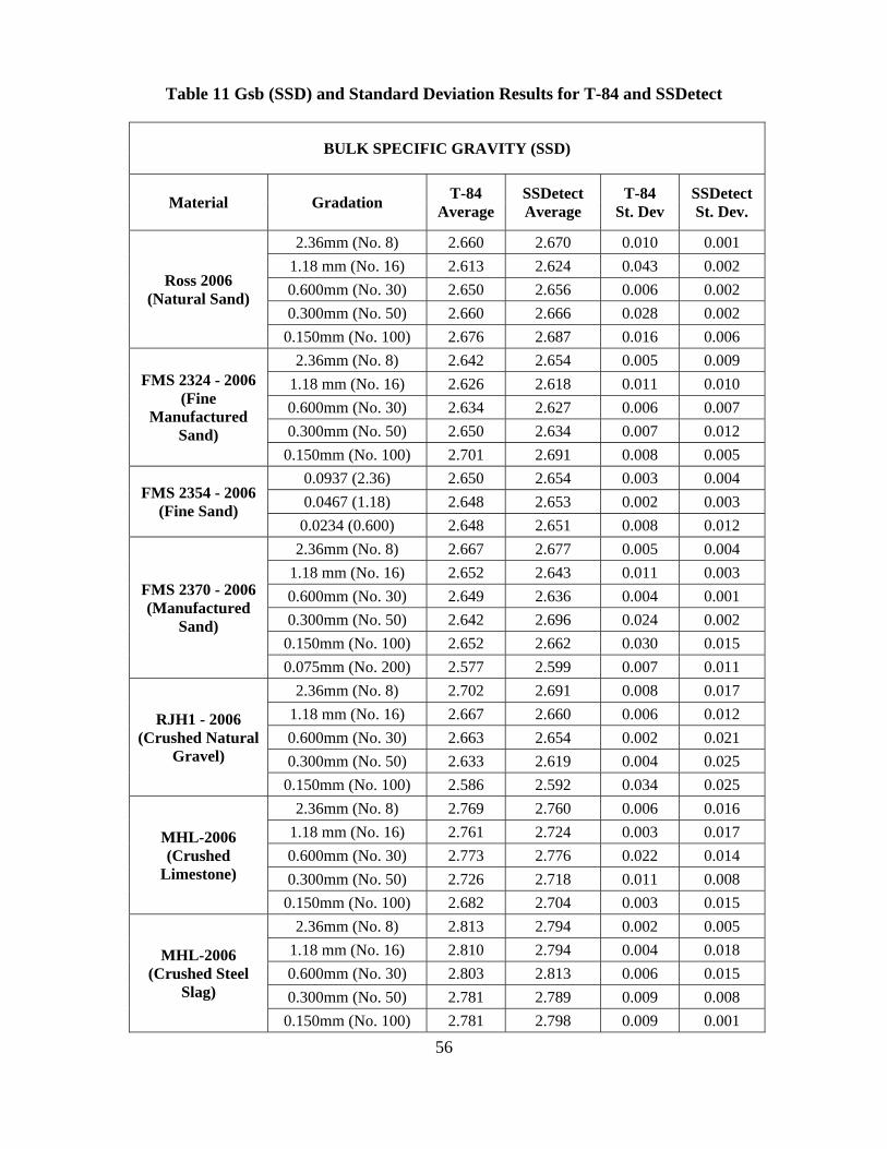
56

Table 11 Gsb (SSD) and Standard Deviation Results for T-84 and SSDetect

BULK SPECIFIC GRAVITY (SSD)


SSDetect Average

T-84 St. Dev

SSDetect St. Dev.



0.150mm (No. 100) 2.676 2.687 0.016 0.006

FMS 2324 - 2006 (Fine

Manufactured Sand)


0.150mm (No. 100) 2.701 2.691 0.008 0.005


0.0937 (2.36) 2.650 2.654 0.003 0.004 0.0467 (1.18) 2.648 2.653 0.002 0.003

0.0234 (0.600) 2.648 2.651 0.008 0.012


Sand)


0.150mm (No. 100) 2.652 2.662 0.030 0.015 0.075mm (No. 200) 2.577 2.599 0.007 0.011


Gravel)


0.150mm (No. 100) 2.586 2.592 0.034 0.025

MHL-2006 (Crushed

Limestone)


0.150mm (No. 100) 2.682 2.704 0.003 0.015


Slag)


0.150mm (No. 100) 2.781 2.798 0.009 0.001

BULK SPECIFIC GRAVITY (SSD)


SSDetect Average

T-84 St. Dev

SSDetect St. Dev.

HMA 5E10 - MLK1 Blended 2.691 2.684 0.014 0.009

HMA 5E10 - MKF2 Blended 2.730 2.707 0.012 0.004

HMA 5E10 - AIF Blended 2.714 2.687 0.008 0.001

HMA 5E10 - NLF Blended 2.707 2.696 0.030 0.002

HMA 4E10 - ARF Blended 2.723 2.731 0.013 0.002

HMA 3E10 - APF Blended 2.702 2.691 0.008 0.011

HMA 2E10 - APF Blended 2.679 2.680 0.019 0.037

HMA 5E3 - GMF Blended 2.667 2.668 0.005 0.002

HMA 4E3 - SLF Blended 2.684 2.657 0.029 0.005

HMA 3E3 - GMF Blended 2.682 2.688 0.005 0.002

57

58

Table 12 Gsa and Standard Deviation Results for T-84 and SSDetect

APPARENT SPECIFIC GRAVITY (Gsa)


SSDetect Average

T-84 St. Dev

SSDetect St. Dev.



0.150mm (No. 100) 2.743 2.720 0.006 0.003

FMS 2324 - 2006 (Fine

Manufactured Sand)


0.150mm (No. 100) 2.777 2.739 0.031 0.005


0.0937 (2.36) 2.764 2.759 0.003 0.008 0.0467 (1.18) 2.783 2.756 0.005 0.004

0.0234 (0.600) 2.774 2.762 0.008 0.009


Sand)


0.150mm (No. 100) 2.754 2.727 0.048 0.009 0.075mm (No. 200) 2.661 2.654 0.007 0.008


Gravel)


0.150mm (No. 100) 2.698 2.677 0.047 0.022

MHL-2006 (Crushed

Limestone)


0.150mm (No. 100) 2.794 2.845 0.020 0.002


Slag)


0.150mm (No. 100) 2.870 2.943 0.010 0.001

APPARENT SPECIFIC GRAVITY (Gsa)


SSDetect Average

T-84 St. Dev

SSDetect St. Dev.

HMA 5E10 - MLK1 Blended 2.750 2.732 0.014 0.009

HMA 5E10 - MKF2 Blended 2.862 2.822 0.007 0.003

HMA 5E10 - AIF Blended 2.791 2.759 0.012 0.002

HMA 5E10 - NLF Blended 2.770 2.768 0.030 0.001

HMA 4E10 - ARF Blended 2.840 2.809 0.004 0.008

HMA 3E10 - APF Blended 2.774 2.803 0.006 0.009

HMA 2E10 - APF Blended 2.769 2.728 0.006 0.005

HMA 5E3 - GMF Blended 2.758 2.732 0.002 0.001

HMA 4E3 - SLF Blended 2.801 2.789 0.036 0.052

HMA 3E3 - GMF Blended 2.772 2.808 0.000 0.001

59

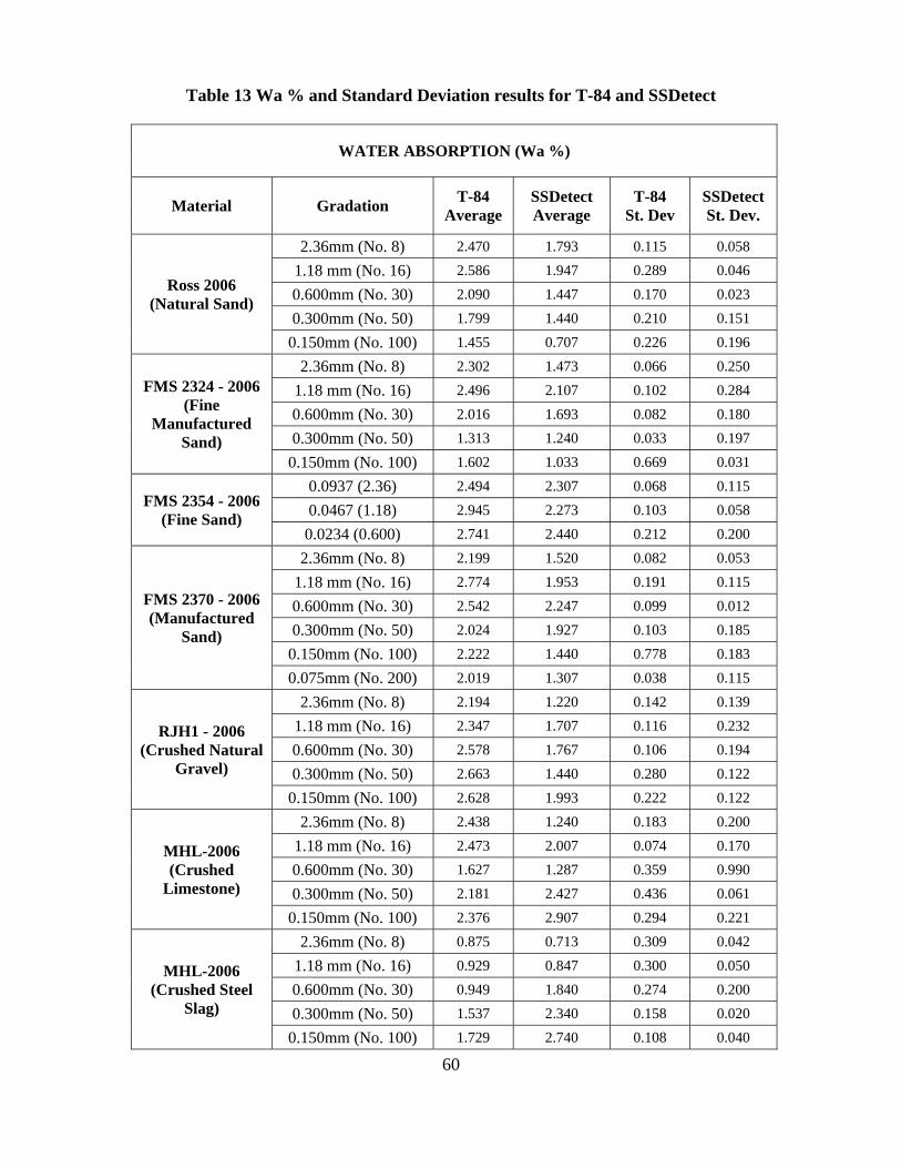
60

Table 13 Wa % and Standard Deviation results for T-84 and SSDetect

WATER ABSORPTION (Wa %)


SSDetect Average

T-84 St. Dev

SSDetect St. Dev.



0.150mm (No. 100) 1.455 0.707 0.226 0.196

FMS 2324 - 2006 (Fine

Manufactured Sand)


0.150mm (No. 100) 1.602 1.033 0.669 0.031


0.0937 (2.36) 2.494 2.307 0.068 0.115 0.0467 (1.18) 2.945 2.273 0.103 0.058

0.0234 (0.600) 2.741 2.440 0.212 0.200


Sand)


0.150mm (No. 100) 2.222 1.440 0.778 0.183 0.075mm (No. 200) 2.019 1.307 0.038 0.115


Gravel)


0.150mm (No. 100) 2.628 1.993 0.222 0.122

MHL-2006 (Crushed

Limestone)


0.150mm (No. 100) 2.376 2.907 0.294 0.221


Slag)


0.150mm (No. 100) 1.729 2.740 0.108 0.040

WATER ABSORPTION (Wa %)


SSDetect Average

T-84 St. Dev

SSDetect St. Dev.

HMA 5E10 - MLK1 Blended 1.275 1.040 0.108 0.002

HMA 5E10 - MKF2 Blended 2.668 2.400 0.127 0.020

HMA 5E10 - AIF Blended 1.612 1.547 0.124 0.042

HMA 5E10 - NLF Blended 1.345 1.520 0.078 0.020

HMA 4E10 - ARF Blended 2.382 1.593 0.212 0.115

HMA 3E10 - APF Blended 1.523 2.367 0.006 0.070

HMA 2E10 - APF Blended 1.937 1.707 0.306 0.220

HMA 5E3 - GMF Blended 1.991 1.420 0.147 0.020

HMA 4E3 - SLF Blended 2.484 2.213 0.779 0.142

HMA 3E3 - GMF Blended 1.930 2.533 0.189 0.061

61

62

APPENDIX B

AASHTO T-84 VERSUS SSDETECT GRAPHICAL PLOTS

63

2.500

2.550

2.600

2.650

2.700

2.750

2.800

2.850

2.500 2.550 2.600 2.650 2.700 2.750 2.800 2.850

AV

ER

AG

E G

sb

(d

ry),

SS

DE

TE

CT

AVERAGE Gsb (dry), AASHTO T84

y = 0.8534x + 0.3904

R2 = 0.925

R2adj = 0.919

Se = 0.0165

Figure 1 AASHTO T-84 against SSDetect Bulk Specific Gravity (dry)

y = 0.9177x + 0.2198

R2 = 0.925

R2adj = 0.923

Se = 0.0165

Figure 2 AASHTO T-84 against SSDetect Bulk Specific Gravity (SSD)

64

65

Figure 3 AASHTO T-84 against SSDetect Bulk Specific Gravity (Gsa)

2.600

2.650

2.700

2.750

2.800

2.850

2.900

2.950

3.000

2.600 2.650 2.700 2.750 2.800 2.850 2.900 2.950 3.000

AV

ER

AG

E G

sa,

SS

DE

TE

CT

AVERAGE Gsa, AASHTO T84

y = 0.9177x + 0.2198

R2 = 0.721

R2adj = 0.715

Se = 0.0165

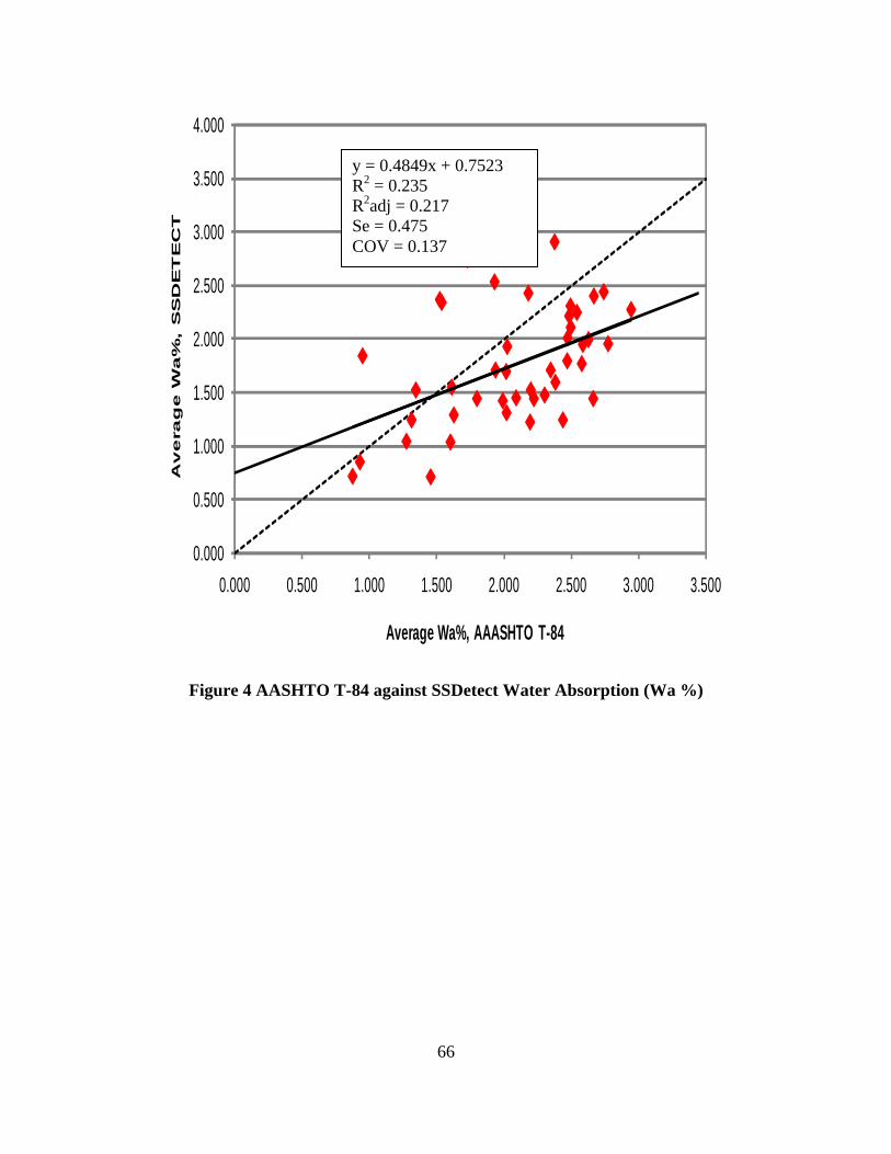
0.000

0.500

1.000

1.500

2.000

2.500

3.000

3.500

4.000

0.000 0.500 1.000 1.500 2.000 2.500 3.000 3.500

Av

era

ge

Wa

%,

SS

DE

TE

CT

Average Wa%, AAASHTO T-84

y = 0.4849x + 0.7523 R2 = 0.235 R2adj = 0.217 Se = 0.475 COV = 0.137

Figure 4 AASHTO T-84 against SSDetect Water Absorption (Wa %)

66

67

Figure 5 Blended-Calculated against SSDetect Gsb (dry)

R² = 0.9468

2.5

2.55

2.6

2.65

2.7

2.75

2.8

2.85

2.5 2.55 2.6 2.65 2.7 2.75 2.8 2.85

BL

EN

DE

D F

INE

S G

sb

(d

ry),

SS

DE

TE

CT

CALCULATED Gsb (dry)

y = 1.0955x + 0.2529

R2 = 0.9287

R2adj = 0.217 Se = 0.475

68

Figure 6 Blended-Calculated against SSDetect Gsb (SSD)

R² = 0.8363

2.5

2.55

2.6

2.65

2.7

2.75

2.8

2.85

2.5 2.55 2.6 2.65 2.7 2.75 2.8 2.85

BL

EN

DE

D F

INE

S G

sb

(S

SD

),S

SD

ET

EC

T

CALCULATED Gsb (SSD)

y = 0.8701x + 0.34

R2 = 0.836 R2adj = 0.752

Se = 0.021

69

Figure 7 Blended-Calculated against SSDetect Gsa

R² = 0.7212

2.6

2.65

2.7

2.75

2.8

2.85

2.6 2.65 2.7 2.75 2.8 2

BL

EN

DE

D G

sa,S

SD

ET

EC

T

CALCULATED Gsa.85

y = 0.7131x + 0.7793 R2 = 0.887 R2adj = 0.878 Se = 0.0149 COV = 0.002

70

R² = 0.6401

0

0.5

1

1.5

2

2.5

3

0 0.5 1 1.5 2 2.5 3

BL

EN

DE

D F

INE

S W

a %

, S

SD

ET

EC

T

CALCULATED Wa %

y = 0.814x + 0.449

R2 = 0.64

R2adj = 0.621 Se = 0.230 COV 0 137

Figure 8 Blended-Calculated against SSDetect Wa%

71

APPENDIX C

AASHTO T-85 VERSUS VACUUM SATURATION TEST GRAPHICAL PLOTS

EXTENDED SOAKING PERIODS FOR COARSE AGGREGATES

Figure 9 AASHTO T-85 versus 10 Minutes Vacuum Saturation Test for Gsb (Dry)

72

Figure 10 AASHTO T-85 against 20 Minutes Vacuum Saturation Test for Gsb (dry)

73

Figure 11 AASHTO T-85 against 30 Minutes Vacuum Saturation Test for Gsb (dry)

74

Figure 12 AASHTO T-85 against 10 Minutes Vacuum Saturation Test for Gsb

(SSD)

75


(SSD)

76


(SSD)

77

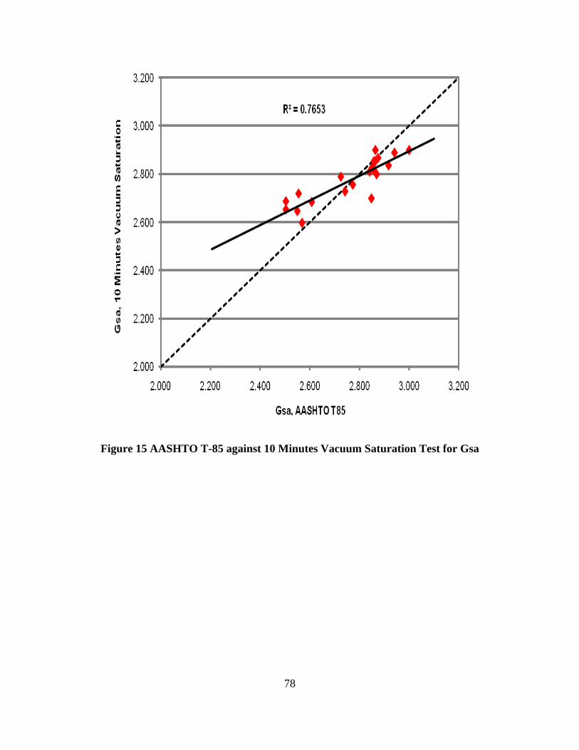
Figure 15 AASHTO T-85 against 10 Minutes Vacuum Saturation Test for Gsa

78


79


80

Figure 18 AASHTO T-85 against 10 Minutes Vacuum Saturation Test for Wa%

81


82


83

R² = 0.8056

2.000

2.200

2.400

2.600

2.800

3.000

2.000 2.200 2.400 2.600 2.800 3.000

Ble

nd

ed

Gsb

(D

ry),

10 M

intu

es V

acu

um

Satu

rati

on

Calculated Gsb (Dry), AASHTO T85

Blended Coarse Aggregates

Figure 21 Gsb (Dry): Calculated Value against Single Test Value of 10 Minutes

Vacuum Saturation Test

84

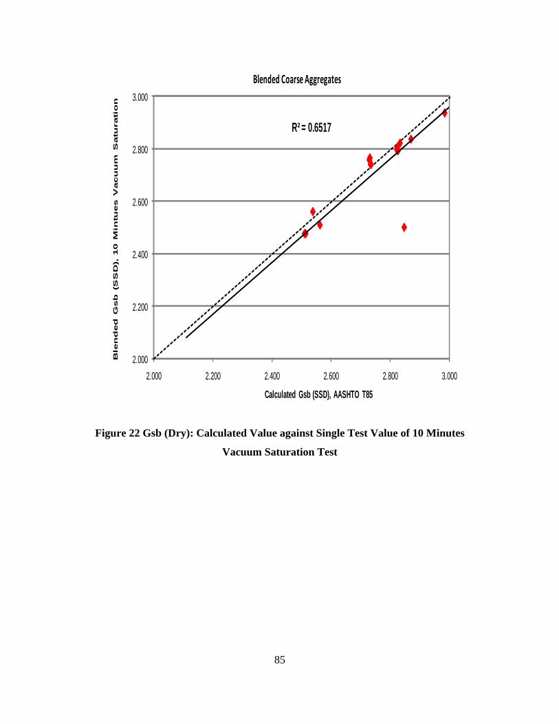
R² = 0.6517

2.000

2.200

2.400

2.600

2.800

3.000

2.000 2.200 2.400 2.600 2.800 3.000

Ble

nd

ed

Gsb

(S

SD

), 1

0 M

intu

es V

acu

um

Satu

rati

on

Calculated Gsb (SSD), AASHTO T85


Figure 22 Gsb (Dry): Calculated Value against Single Test Value of 10 Minutes

Vacuum Saturation Test

85

Figure 23 Gsa: Calculated Value against Single Test Value of 10 Minutes Vacuum

Saturation Test

R² = 0.4449

2.500

2.750

3.000

3.250

3.500

2.500 2.750 3.000 3.250 3.500

Ble

nd

ed

Gsa,

10 M

intu

es V

acu

um

Satu

rati

on

Calculated Gsa, AASHTO T85


86

R² = 0.9752

0.000

1.000

2.000

3.000

4.000

5.000

6.000

7.000

8.000

0.000 1.000 2.000 3.000 4.000 5.000 6.000 7.000 8.000

Ble

nd

ed

Wa%

, 10 M

intu

es V

acu

um

Satu

rati

on

Calculated Wa%, AASHTO T85


Figure 24 Wa%: Calculated Value against Single Test Value of 10 Minutes Vacuum

Saturation Test

87

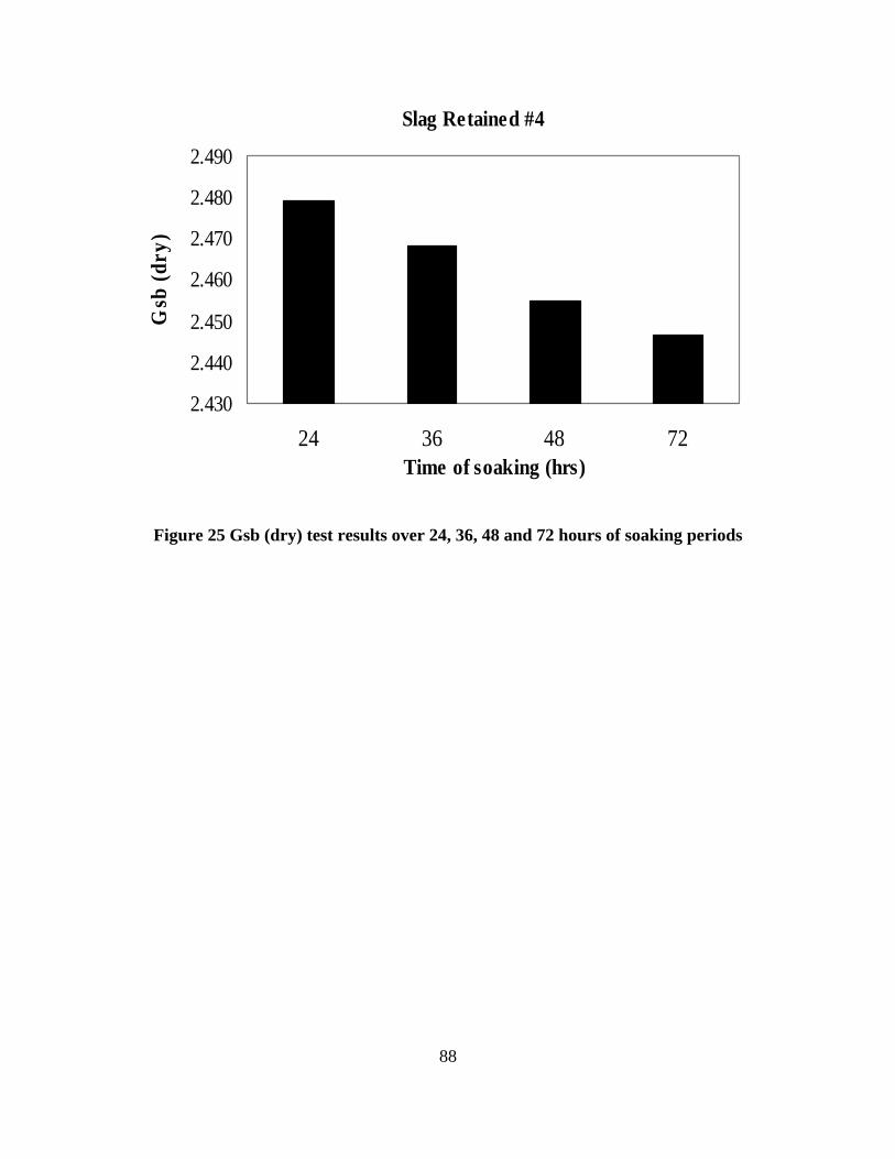
Slag Retained #4

2.430

2.440

2.450

2.460

2.470

2.480

2.490

24 36 48 72Time of soaking (hrs)

Gsb

(dry

)

Figure 25 Gsb (dry) test results over 24, 36, 48 and 72 hours of soaking periods

88

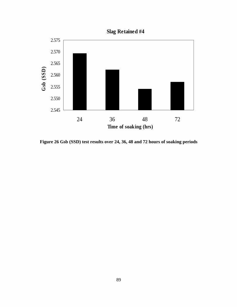
Slag Retained #4

2.545

2.550

2.555

2.560

2.565

2.570

2.575


Gsb

(SSD

)

Figure 26 Gsb (SSD) test results over 24, 36, 48 and 72 hours of soaking periods

89

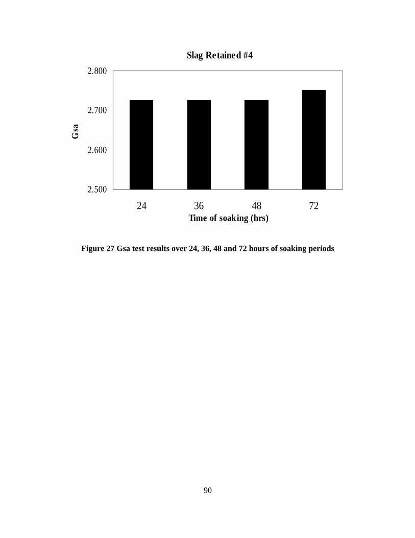
Slag Retained #4

2.500

2.600

2.700

2.800


Gsa

Figure 27 Gsa test results over 24, 36, 48 and 72 hours of soaking periods

90

Slag Retained #4

2.500

2.600

2.700

2.800


Wa%

Figure 28 Wa% test results over 24, 36, 48 and 72 hours of soaking periods

91

rc-1535 - development of new test procedures for · pdf filemeasuring fine and coarse...

Documents