Ray Optics and Heat Transfer Analysis of a Curved Fresnel Lens Heater for a Desalination System Laura Mabel Almara1 1. Department of Mechanical Engineering, University of North Texas, Denton, TX, USA. lauraalmara@my.unt.edu Abstract

This paper uses COMSOL Multiphysics® to investigate, analyze and simulate a system composed of a Fresnel lens, a heat receiver and a heating chamber. The project provides the energy to a solar powered desalination system, where the input is seawater, and the output is drinking water. The lens is curved, made of PMMA, 120 cm diameter. The receiver and the chamber are made of copper.

This study comprises two parts. The heat transfer simulation considers only the receiver and the chamber, using a Gaussian Function on the receiver surface to simulate the sunlight energy. The ray heating simulation includes lens, receiver and chamber.

The results show temperatures and heat flux values. The same simulations were performed for a flat Fresnel lens of the same diameter. Comparative analysis and discussion are provided. Keywords

Curved Fresnel lens, flat Fresnel lens, prism groove, desalination system, seawater, heater, receiver, COMSOL Multiphysics, simulation, heat transfer, ray heating, ray trajectory, solar irradiation, heat flux, Gaussian Function, Gaussian Pulse, Geometrical Optics, Ray Optics, Ray Heat Source. Introduction

Fresnel lenses have wide applications; one of them is to concentrate energy. Seawater can be converted into fresh water using solar energy. This is as an easy, suitable and green solution method to obtain heat for desalination. It is possible to concentrate the sunlight heat flux onto a small focal area by using a Fresnel lens. When the focal area is correctly located to an evaporation chamber, the obtained heat from the sun can significantly increase the temperature, and therefore evaporate the water, separating the salt. This water steam can be condensed to produce fresh water for human consumption.

Seawater has an average salinity of 35 parts per thousand (35 g/l), and its boiling point is at 373.15 K (100 °C). The melting point of copper is at 1,358.15 K (1,085 °C).

Depending on the requirements of fresh water output as a function of time, it is necessary to design the lens to obtain the expected heat at the receiver surface, and dimension the chamber in order to have an energy distribution on the entire evaporating chamber.

This project is about simulating an efficient and portable solar technology desalination to obtain drinking water. The heater system has an internal core to act as the energy supplier for the chamber. The design and size of the core are determined by the amount of heat that it can transport and distribute to the chamber, where a uniform distribution of the heat is an important aspect. A 120 cm diameter curved PMMA (Polymethyl methacrylate) Fresnel lens is used to concentrate energy from incoming sunlight on the receiver focal plane, which is 10 cm diameter, distributing it to the core of the water heater. The entire system was set to work at ambient temperature. The rod is 30 cm height; the receiver thickness is 0.2 cm. In order to analyze and test this project, a simulation using COMSOL Multiphysics® was used. A comparison with Flat Fresnel lens is provided.

Curved Fresnel lens

The simulation and analysis on this work includes a 120

cm diameter PMMA Fresnel lens and a copper chamber, with the receiver at the top of it.

Figure 1. System components.

The chamber has fins equally distributed along the total height of a rod, with holes that allow the seawater to drip downward from one fin to another, to easy the evaporation. The hollow rod has a height of 0.3 m plus a top thin plate receiver of 0.002 m. At the bottom of the rod, there is a thin plate base of 0.0064 m thickness.

Figure 2. a) Chamber, b) Hollow rod and receiver designs. Design Parameters and Material Properties

Copper was used for the chamber and the receiver, and PMMA for Fresnel lens.

Figure 3 illustrates a diagram with the main curved Fresnel lens parameters.

Figure 3. Parameters of curved Fresnel lens design.

Table 1 lists the design parameters and Table 2 the material properties considered. Table 1: Design parameters

Table 2: Material Properties

Computational Methods

This work includes two computational methods: 1. Computational Analysis: Curved Fresnel lens was designed based on an

algorithmic method using MATLAB[1], which provides the high optimization lens measurements, giving the optimum number of grooves and dimensions of each groove, where each

groove has different dimensions along the lens. Then it was drawn with CAD software.

2. Simulation Analysis: The Fresnel lens and chamber, including the core rod and

receiver were simulated in COMSOL Multiphysics®. Appling Heat Transfer in Solids analysis, from the Fluid Flow and Heat Transfer Module, it was possible to simulate heat propagation and distribution in the system. With Ray Optics, from the Electromagnetics Module, using Geometrical Optics, it was possible to simulate ray trajectories. Ray Heating simulation combines Heat Transfer and Geometrical Optics analysis, by using Ray Heat Source from Multiphysics Couplings.

Simulation Methods

This work includes two types of COMSOL simulations: 1. Heat Transfer in Solids: Simulates only the temperature propagation and

distribution in the heating chamber using a Gaussian Pulse to simulate the sunrays energy (heat flux) applied to the receiver. The Gaussian function parameters were calculate running an algorithmic method using MATLAB[1]. This provides an idealized result.

2. Ray Heating (Ray Optics): Simulates the chamber and lens heat propagation and

distribution due to sunrays, real sunrays energy (heat flux) applied on the receiver and ray trajectories. This simulation provides results that resemble real behavior.

The parts of the chamber were drawn in 3D in COMSOL, and the Fresnel lens was imported as STL file. From the Material Library, copper was selected for the receiver, core and chamber and PMMA for the lens. Extremely Fine Free Tetrahedral mesh size was used for the receiver's surface. Heat Transfer and Ray Heating simulations were run on a 4 hours Time Dependent study. Governing Equations

The main equations used in Heat Transfer for heat flux in

these simulations are:

Convective heat flux: 푞 = ℎ ∙ (푇 − 푇) (1) General inward heat flux: 푞 = gop.wall2.bsrc1.Qp (2)

Initial Conditions

1. Heat Transfer in Solids: The domain selection includes the entire system. The

initial temperature value was 293.15 K. There are no thermal insulation selections.

a b

H

2. Geometrical Optics: The domain selection includes only the Fresnel lens. The

wavelength distribution of released rays is monochromatic. For intensity computation, it was selected “Compute intensity and power”.

The values of the parameters used in Heat Transfer and Geometrical Optics are listed in Tables 3 and 4, respectively. Air was used as fluid.

푃 = 퐼 ∙ 퐴푟푒푎 (3) 퐴푟푒푎 = 휋 ∙ (푅푎푑푖푢푠 ) (4) Table 3: Heat Transfer parameters

Table 4: Geometrical Optics parameters

Boundary Conditions

1. Heat Transfer in Solids: Different Heat Flux boundaries were defined for each

component, where the heat transfer coefficients for each component was selected depending on the shape.

In the case for Heat Transfer, which considers only the chamber and receiver, a Gaussian Pulse function was used to simulate the sunrays energy on the receiver. The fifth order Gaussian Function was placed in the general inward heat flux. The boundary selection was the receiver surface.

2. Geometrical Optics: Boundary Illuminated Surface feature was used on the

lens surface top, which simulates the release sunrays. Freeze Wall boundary condition was used on the receiver surface, which stops the sunrays from the lens. Deposited Ray Power boundary selection was applied on the receiver surface.

Results

1. Heat Transfer in Solids: Only the chamber was simulated applying Heat Transfer

simulation and setting Gaussian Function at the receiver surface. The Gaussian Function output from MATLAB code is fifth order, and applying it along the receiver surface, it shows a peak of 612057.5 W/m2.

Figure 4. 3D Receiver Surface Inward Heat Flux Distribution using Gaussian Function.

The maximum and minimum temperatures obtained for 4

hours were 679.94 and 354.22 K. The minimum temperature is located on the last fin edge. See Figure 5. The temperature distribution along the receiver surface is concentric with a peak of 680.07 K, minimum of 532.32 K, and follows the shape of the Gaussian Function. See Figure 6.

Heat flux had a peak of 6.15x105 W/m2 on the 2D plot, Figure 7, being very similar in value to the 612057.5 W/m2 obtained on the 3D plot of Figure 4.

Figure 5. 3D Chamber Temperature Distribution using Heat Transfer by applying Gaussian Function.

Figure 6. 2D Receiver Surface Temperature Distribution using Heat Transfer by applying Gaussian Function.

Figure 7. 2D Receiver Surface Heat Flux Distribution using Gaussian Function.

2. Ray Heating: The total system was simulated, lens and chamber,

applying Ray Heating. In this case, Figure 8 shows the maximum and minimum temperatures obtained for 4 hours were 898.07 and 363.93 K, where the minimum temperature of the chamber is located on the last fin edge. The minimum temperature of the system is in the lens with 293.15 K. As in Heat Transfer simulation, the temperature distribution along the receiver surface is concentric with a peak of 902.67 K, following the shape of the Gaussian Function, Figure 9. Heat flux had a peak of 3.63x106 W/m2 on the 2D plot, along the receiver surface, Figure 10. As Ray Heating simulation is more close to reality compared to only Heat Transfer, the peak value of temperature and heat flux are higher. The ray trajectories have very good concentric focus on the receiver surface.

Figure 8. 3D Temperature Distribution and Ray Trajectory using Ray Heating.

Figure 9. 2D Receiver Surface Temperature Distribution using Ray Heating.

Figure 10. 2D Receiver Surface Heat Flux Distribution using Ray Heating.

Figure 11 shows the decreasing temperature on the receiver as function of its depth. From the top of the receiver surface to the plane that starts the rod surface, it is losing approximate 7 K.

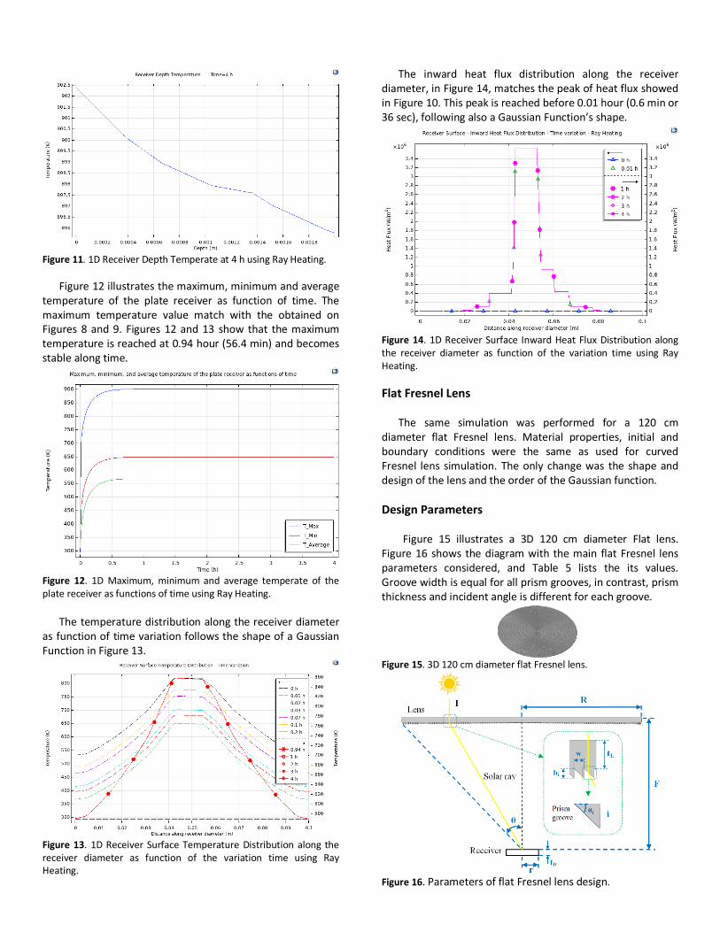
Figure 11. 1D Receiver Depth Temperate at 4 h using Ray Heating.

Figure 12 illustrates the maximum, minimum and average temperature of the plate receiver as function of time. The maximum temperature value match with the obtained on Figures 8 and 9. Figures 12 and 13 show that the maximum temperature is reached at 0.94 hour (56.4 min) and becomes stable along time.

Figure 12. 1D Maximum, minimum and average temperate of the plate receiver as functions of time using Ray Heating.

The temperature distribution along the receiver diameter

as function of time variation follows the shape of a Gaussian Function in Figure 13.

Figure 13. 1D Receiver Surface Temperature Distribution along the receiver diameter as function of the variation time using Ray Heating.

The inward heat flux distribution along the receiver diameter, in Figure 14, matches the peak of heat flux showed in Figure 10. This peak is reached before 0.01 hour (0.6 min or 36 sec), following also a Gaussian Function’s shape.

Figure 14. 1D Receiver Surface Inward Heat Flux Distribution along the receiver diameter as function of the variation time using Ray Heating. Flat Fresnel Lens

The same simulation was performed for a 120 cm

diameter flat Fresnel lens. Material properties, initial and boundary conditions were the same as used for curved Fresnel lens simulation. The only change was the shape and design of the lens and the order of the Gaussian function.

Design Parameters

Figure 15 illustrates a 3D 120 cm diameter Flat lens. Figure 16 shows the diagram with the main flat Fresnel lens parameters considered, and Table 5 lists the its values. Groove width is equal for all prism grooves, in contrast, prism thickness and incident angle is different for each groove.

Figure 15. 3D 120 cm diameter flat Fresnel lens.

Figure 16. Parameters of flat Fresnel lens design.

Table 5: Design parameters

Where: 퐹표푐푎푙 푙푒푛푔푡ℎ = 퐹 = 2 ∙ 푅 (5) Results

1. Heat Transfer in Solids:

The Gaussian Function output from MATLAB code is of third order. Applying this function along the receiver surface a peak of 1253292.4 W/m2 is obtained, being higher than 612057.5 W/m2 from heat transfer using a curved Fresnel lens. The peaks from MATLAB and 3D COMSOL Gaussian Function, Figure 17 Left and Right, match in value and shape.

Figure 17. Left: 1D heat flux along the receiver surface distribution due to third order Gaussian Function for a 120 cm diameter flat Fresnel lens by MATLAB. Right: 3D Receiver Surface Inward Heat Flux Distribution using Gaussian Function.

For 4 hours simulation, the maximum and minimum temperatures obtained were 927.03 and 390.51 K. See Figure 18. Like in curved lens, the minimum temperature is located on the last fin edge. The temperature distribution along the receiver surface is concentric with a peak of 927.3 K and has a minimum of 677.29, following the shape of the Gaussian Function. See Figure 19 Left. The maximum temperature is higher than obtained using a curved lens. Heat flux had a peak of 1.256x106 W/m2 on the 2D plot, Figure 19 Right, which is similar in value to the 1253292.4 W/m2 obtained on the 3D plot in Figure 17 Right, and higher compared to the use of a curved lens.

Figure 18. 3D Chamber Temperature Distribution using Heat Transfer by applying Gaussian Function.

Figure 19. Left: 2D Receiver Surface Temperature Distribution using Heat Transfer by applying Gaussian Function. Right: 2D Receiver Surface Heat Flux Distribution using Gaussian Function.

2. Ray Heating:

As in Ray Heating simulation for curved lens, the peak value of temperature and heat flux are higher compared to Heat Transfer simulation.

There is a concentric focus on the receiver surface of ray trajectories. For 4 hours simulation, the maximum and minimum temperatures were 794.39 and 362.96 K, where the minimum temperature of the chamber is also located on the last fin edge. The minimum temperature of the system is at the lens, with 293.15 K. Curved lens provides higher maximum temperature compared to flat lens; however in both cases the minimum temperatures are very similar in value. The temperature distribution along the receiver surface is concentric with a peak of 798.33 K, and follows the shape of the Gaussian Function. See Figure 21 Left.

The heat flux obtained has a peak of 2.32x106 W/m2 on the 2D plot, along the receiver surface, Figure 21 Right, which is, in value, lower than using a curved lens.

Figure 20. 3D Temperature Distribution and Ray Trajectory using Ray Heating.

Figure 21. Left: 2D Receiver Surface Temperature Distribution using Ray Heating. Right: 2D Receiver Surface Heat Flux Distribution using Ray Heating.

The decreasing temperature on the receiver as function of its depth figure shows that from the top of the receiver surface to the plane that starts the rod surface, is losing approximate 5 K. See Figure 22 Left.

Figure 22. Left: 1D Receiver Depth Temperate at 4 h using Ray Heating. Right: 1D Maximum, minimum and average temperate of the plate receiver as functions of time using Ray Heating.

According to Figure 22 Right, the maximum temperature value matches the obtained in Figures 20 and 21 Left. In flat lens, the temperature was reached at 0.72 hour (43.2 min) (acquiring stability through time), Figure 23, following the shape of a Gaussian Function on the receiver surface.

Figure 23. 1D Receiver Surface Temperature Distribution along the receiver diameter as function of the variation time using Ray Heating.

As in curved lens, the inward heat flux distribution along the receiver diameter illustrated in Figure 24, matches the peak of heat flux in Figure 21 Right. This peak is reached before 0.01 hour (0.6 min or 36 sec), following also a Gaussian Function’s shape.

Figure 24. 1D Receiver Surface Inward Heat Flux Distribution along the receiver diameter as function of the variation time using Ray Heating.

Table 5 shows the summary of the main results obtained from heat transfer and ray heating simulations for a 120 cm

diameter curved and flat Fresnel lenses. In heat transfer simulation, flat lens achieved the higher temperature at the receiver surface and at the entire system. In contrast, in ray heating simulation, curved lens achieved the higher temperature. The same behavior happens in terms of heat flux, where in heat transfer the flat lens has the higher value, and in ray heating, curved lens has the higher value. Using a flat lens, the maximum temperature is reached faster than using a curved lens. Table 5: Summary of Main Results

Conclusions

The objective of this work is to predict temperature and heat flux values on the receiver surface. The designs of the water evaporating chamber and lens depend on the freshwater output requirements.

The results of this work will be used to analyze the best chamber design and diameter of curved or flat Fresnel lens, according to the fresh water output requirements with the purpose to generate a prototype.

Ray Heating simulations show that curved lens provides higher values compared to heat transfer simulations.

Results of temperature and heat flux values on the receiver surface obtained in this study can be used as a reference to investigate and apply in other Fresnel lens applications.

Further work will continue with the fabrication of a prototype. References [1] H. Qandil, W. Zhao, Design and Evaluation of the Fresnel-Lens Based Solar Concentrator System through a Statistical-Algorithmic Approach, Proceedings of IMECE 2018, 87023, (2018) Acknowledgements Dr. W. Zhao and Dr. H. Qandil provided access the MATLAB code for the Gaussian Functions used in the Heat Transfer simulation and design optimization of lenses.