randomized and deterministic primality testing - algo

Ecole Polytechnique Fédérale de Lausanne

Bachelor semester project:Randomized and Deterministic PrimalityTesting

Monica Perrenoud

Under the direction of

Professor Mohammad Amin ShokrollahiResponsible assistant Ghid Maatouk

Fall 2009

Abstract

This project presents some randomized and deterministic algorithmsof number primality testing, and, for some of them, their implementa-tion in C++.The algorithms studied here are the naive algorithm (deterministic),the Miller-Rabin algorithm (randomized), the Fermat algorithm (ran-domized), the Solovay-Strassen algorithm (randomized) and the AKSalgorithm (deterministic).These algorithms are presented with the number theory they need tobe understood and with some proofs of the theorems they use.

1

Contents

1 Introduction 4

2 General informations about the algorithms 5

2.1 Deterministic and randomized algorithms . . . . . . . . . . . 52.2 Density of prime numbers . . . . . . . . . . . . . . . . . . . . 52.3 Output of the algorithms . . . . . . . . . . . . . . . . . . . . 52.4 Running time . . . . . . . . . . . . . . . . . . . . . . . . . . . 6

3 The naive algorithm 7

3.1 General idea . . . . . . . . . . . . . . . . . . . . . . . . . . . . 73.2 More precisely . . . . . . . . . . . . . . . . . . . . . . . . . . 73.3 Running time . . . . . . . . . . . . . . . . . . . . . . . . . . . 8

4 The Miller-Rabin algorithm 9

4.1 Number theory for the Miller-Rabin algorithm . . . . . . . . 94.1.1 Carmichael numbers . . . . . . . . . . . . . . . . . . . 12

4.2 General idea . . . . . . . . . . . . . . . . . . . . . . . . . . . . 174.3 More precisely . . . . . . . . . . . . . . . . . . . . . . . . . . 184.4 Running time . . . . . . . . . . . . . . . . . . . . . . . . . . . 194.5 Analysis of the errors . . . . . . . . . . . . . . . . . . . . . . . 19

5 The Fermat algorithm 22

5.1 General idea . . . . . . . . . . . . . . . . . . . . . . . . . . . . 225.2 More precisely . . . . . . . . . . . . . . . . . . . . . . . . . . 225.3 Running time . . . . . . . . . . . . . . . . . . . . . . . . . . . 22

6 The Solovay-Strassen algorithm 24

6.1 Number theory for the Solovay-Strassen algorithm . . . . . . 246.2 General idea . . . . . . . . . . . . . . . . . . . . . . . . . . . . 286.3 More precisely . . . . . . . . . . . . . . . . . . . . . . . . . . 286.4 Running time . . . . . . . . . . . . . . . . . . . . . . . . . . . 296.5 Number of non-witnesses . . . . . . . . . . . . . . . . . . . . . 31

7 The AKS algorithm 33

7.1 Number theory for the AKS algorithm . . . . . . . . . . . . . 337.2 The algorithm . . . . . . . . . . . . . . . . . . . . . . . . . . . 347.3 Running time . . . . . . . . . . . . . . . . . . . . . . . . . . . 347.4 Correctness . . . . . . . . . . . . . . . . . . . . . . . . . . . . 35

8 Comparison of the algorithms 41

Appendices 44

2

A Implementations in C++ 44

A.1 Fermat algorithm implementation . . . . . . . . . . . . . . . . 44A.2 Miller-Rabin algorithm implementation . . . . . . . . . . . . 45A.3 Solovay-Strassen algorithm implementation . . . . . . . . . . 47A.4 Implementation of the comparison of the algorithms . . . . . 49

References 54

3

1 Introduction

For many applications (as cryptography), it is very useful to find large primenumbers. But the problem is to find these large prime numbers. Somealgorithms have been developed to check if a given large number is prime ornot. Some of them make the study of this project.Some of these algorithms do not give a sure answer, they only give it with acertain probability (which can be very high if we iterate a lot the algorithm).But we can study how many errors they make (in comparison to the naivealgorithm) and what can be done to make these errors as small as possible.This is the case for the Miller-Rabin, the Fermat and the Solovay-Strassenalgorithm.The AKS algorithm is interesting in an other way. It is more theoreticalthan practical. The problem of finding if an algorithm of primality testingcan be in P (so which runs in polynomial time) was resolved a little timeago. This algorithm is the AKS algorithm which is presented here with theexplanation of its running time and correctness.All of the algorithms of primality testing are based on some elements ofnumber theory. Here are presented some of these elements that are used inthe studied algorithms and are necessary to understand them.Note that this subject makes sense only in N. So all the numbers, unlessotherwise specified, are taken in N.

4

2 General informations about the algorithms

2.1 Deterministic and randomized algorithms

There are two types of algorithms: deterministic and randomized.A deterministic algorithm is an algorithm that behaves predictably. Wecan run it as many times we want, with the same input, it will always dothe same steps and give the same answer.But a randomized algorithm is an algorithm that uses some randomvalues in hope to verify a property in the average case. Since it is not possibleto have random numbers, the randomized algorithms use a pseudorandomgenerator of numbers. If the probability to find a number verifying theproperty is rather good, we say that it is a good randomized algorithm.

2.2 Density of prime numbers

To ensure that the randomized algorithms can work in a little time, we haveto look at the density of prime numbers.

Definition 2.2.1

The distribution function of prime numbers is written π(n) and spec-ifies the quantity of prime numbers less than or equal to n.

Theorem 2.1 (Prime number theorem)A good approximation of π(n) is given by:

limn→∞

π(n)� nlnn� = 1.

So we can estimate that a number a ∈ N randomly chosen has a proba-bility of 1

ln a to be prime. If we randomly take a number a, we will have totest about ln a numbers around a to find a prime number of the same lengthof a.

2.3 Output of the algorithms

The output of the algorithms seen in this project is, for an input n ∈ N, ifn is prime or composite.But not in all algorithms the output is right at 100%. Some of them arebased on some criterion that ensures with a certain probability that theanswer is right. In our case, when the algorithm gives the answer thata number is composite, then it is really composite. But if the algorithmgives the answer that this number is prime, this means that this number isprime with a certain (high) probability (but it can be composite). It is thecase for the Miller-Rabin, the Fermat and the Solovay-Strassen algorithms.With them, we can determine if a number is composite, but only say that

5

a number have a certain probability to be prime because it passes a certainnumber of tests. These tests are criteria for the number not to be prime.The goal of these algorithms is to have a high probability for a number tobe prime in a few tests.The naive algorithm and the AKS algorithm give a "sure" answer. So if suchan algorithm gives us the answer that a certain number is prime (respectivelycomposite), then this number is really prime (that is sure) (respectivelycomposite).

2.4 Running time

In this project, the running time of the algorithms is analyzed. They aregiven in function of the binary length of their input n ∈ N (written len(n)).

6

3 The naive algorithm

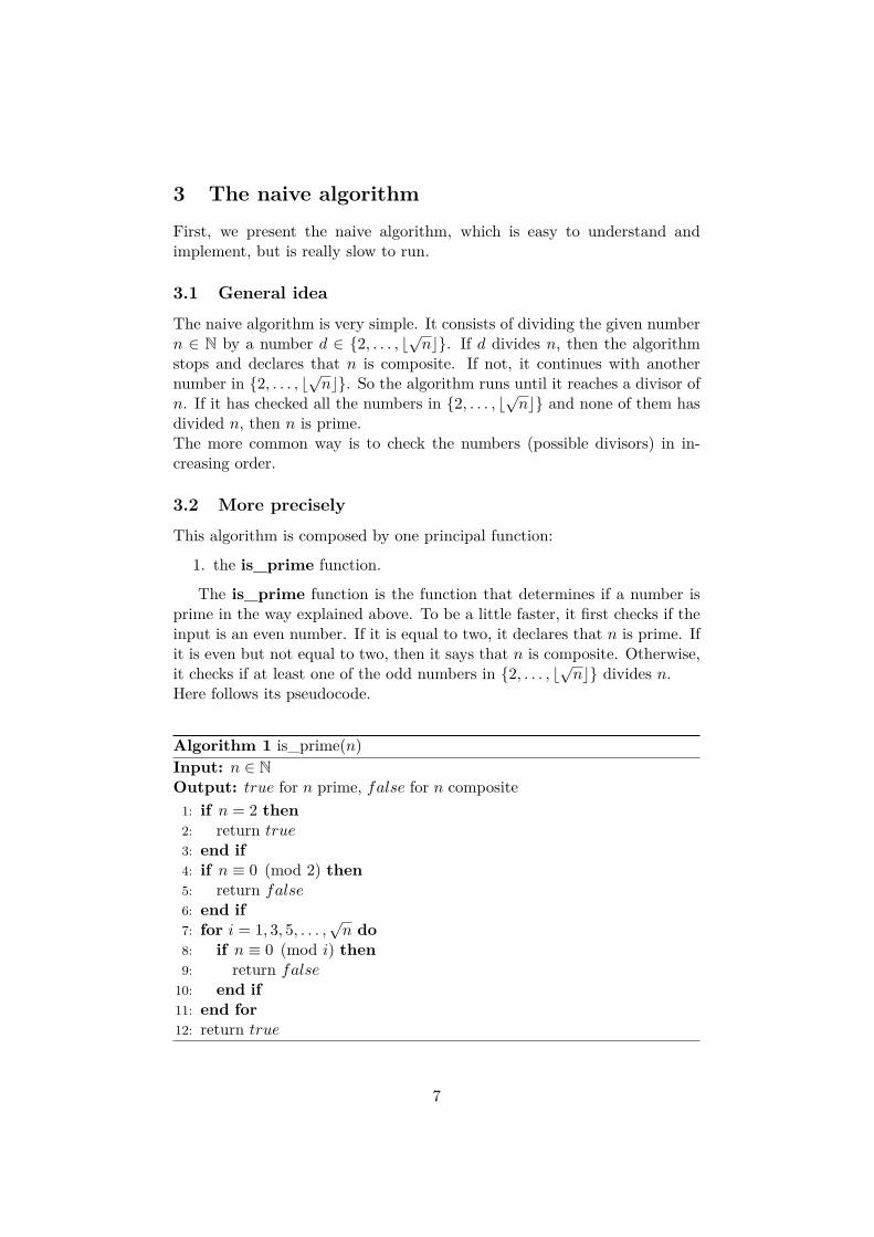
First, we present the naive algorithm, which is easy to understand andimplement, but is really slow to run.

3.1 General idea

The naive algorithm is very simple. It consists of dividing the given numbern ∈ N by a number d ∈ {2, . . . , �

√n�}. If d divides n, then the algorithm

stops and declares that n is composite. If not, it continues with anothernumber in {2, . . . , �

√n�}. So the algorithm runs until it reaches a divisor of

n. If it has checked all the numbers in {2, . . . , �√n�} and none of them has

divided n, then n is prime.The more common way is to check the numbers (possible divisors) in in-creasing order.

3.2 More precisely

This algorithm is composed by one principal function:

1. the is_prime function.

The is_prime function is the function that determines if a number isprime in the way explained above. To be a little faster, it first checks if theinput is an even number. If it is equal to two, it declares that n is prime. Ifit is even but not equal to two, then it says that n is composite. Otherwise,it checks if at least one of the odd numbers in {2, . . . , �

√n�} divides n.

Here follows its pseudocode.

Algorithm 1 is_prime(n)Input: n ∈ NOutput: true for n prime, false for n composite

1: if n = 2 then

2: return true3: end if

4: if n ≡ 0 (mod 2) then

5: return false6: end if

7: for i = 1, 3, 5, . . . ,√n do

8: if n ≡ 0 (mod i) then


11: end for

12: return true

7

3.3 Running time

The advantage of this algorithm is that it never gives a false answer, but forlarge numbers, this algorithm is really slow. For exemple, if n is an integerof length β bits (which means that β = �log2 n�), then the algorithm hasa running time in O(

√n) = O(

√2β) = O(2

β2 ), which is exponential in the

length of n.

8

4 The Miller-Rabin algorithm

To understand and implement this algorithm, I based my researches on [1].

4.1 Number theory for the Miller-Rabin algorithm

Definition 4.1.1

We define Zn byZn = {0, 1, . . . , n− 1}.

AndZ+n = Zn \ {0}.

Then if n is prime, we have Z+n = Z∗n, where Z∗n is the set of the invertible

elements of Zn.We can also see that with the usual addition and multiplication Z+

n is a ringand Z+

p is a field for p prime.

Theorem 4.1 (Chinese remainder theorem)Let n = n1 · . . . · nk be an integer where the ni are pairwise relatively prime.Then

Zn ∼= Zn1 × · · ·× Znk . (1)

Proof. We can say that n = n1 · m with m = n2 · . . . · nk and m and n1relatively prime. So we can prove the theorem for k = 2 and then prove therest by induction over k.We suppose that n = n1 · n2 with n1 and n2 relatively prime. That meansthat n1Z + n2Z = gcd(n1, n2)Z = Z. So there exist some u and v in Z suchthat un1 + vn2 = 1 (this result is called Bezout’s theorem). To simplify wecall b1 = un1 and b2 = vn2.Let π : Z → Zn1 , a �→ a and ρ : Z → Zn2 , a �→ a be the two canonichomomorphisms. We consider now the homomorphism

φ : Z→ Zn1 × Zn2 , a �→ (a, a).

We clearly see that kerφ = n1n2Z = nZ.We want to show that φ is surjective. Let (x, y) ∈ Zn1 × Zn2 . And leta = yb1 + xb2 (where x is a preimage of x by the canonic homomorphism πand y is a preimage of y by the canonic homomorphism ρ). Then workingin Zn1 , we have

a = yb1 + xb2 = yb1 + xb2 = yun1 + xvn2 = yu0 + xvn2 = xb2= x(1− b1) = x(1− un1) = x(1− un1) = x− xun1 = x.

Similarly, working in Zn2 , we have a = y too. So we have shown that(a, a) = φ(a) = (x, y), which implies that φ is surjective.We can now apply the first isomorphism theorem, which tells us that

Zn ∼= Zn1 × Zn2 .

9

We can repeat this theorem into the following corollary.

Corollary 4.2

Let n1 and n2 be two integers which are relatively prime. Then for somegiven a and b, we can solve the following congruence relations:

�x ≡ a (mod n1)x ≡ b (mod n2).

And the solution is unique modulo n1n2.

Corollary 4.3

Let n1 and n2 be two integers which are relatively prime and such thatn = n1n2. Then for some given x and a, we have:

�x ≡ a (mod n1)x ≡ a (mod n2)

if and only ifx ≡ a (mod n).

These two corollaries can be generalized for n1, . . . , nk some integerswhere the ni are pairwise relatively prime.

Definition 4.1.2

The Euler totient function φ(n) is the number of integers less than orequal to n which are relatively prime to n.

Properties 4.4

The totient function has the following properties:

• φ(p) = p− 1 for each p prime;

• φ(pe) = pe−1(p− 1) for each p prime and each e integer;

• φ(mn) = φ(m) · φ(n) for each m and n relatively prime.

Theorem 4.5 (Euler’s theorem)Let n be an integer. Then for every a ∈ Z+

n with a and n relatively prime,n verifies the following equation:

aφ(n) ≡ 1 (mod n). (2)

Proof. Since gcd(a, n) = 1, we have (using again Bezout’s theorem seenin the proof of the Chinese remainder theorem, theorem 4.1) that a is anelement of Z∗n. And the reciprocal is true too (with the same arguments).This implies that φ(n) = |Z∗n|.

10

Let �a� be the subgroup of Z∗n generated by a and let d be its order. Weknow that d divides |Z∗n| (result called Lagrange’s theorem). So there existsa k ∈ N such that d · k = |Z∗n|.By the definition of the order, we have ad = 1. So we have

aφ(n) = a|Z∗n| = ad·k = (ad)k = 1k = 1

(all equations done in Zn).

Theorem 4.6 (Fermat’s little theorem)Let p be a prime number. Then for every a ∈ Z∗p, p verifies the followingequation:

ap−1 ≡ 1 (mod p).

Proof. Since a lies in Z∗p, we have that gcd(a, p) = 1. Then by the propertiesof the totient function, we know that p prime implies that φ(p) = p−1. Thenusing Euler’s theorem, we have

ap−1 = aφ(p) ≡ 1 (mod p).

Theorem 4.7

Let n be an integer. Then

{a ∈ Z∗n : an−1 ≡ 1 (mod n)} ≤ Z∗n,

where ≤ means "to be a subgroup of".Proof. Let a, a1, a2 ∈ (Z/nZ)∗ be such that an−1 ≡ 1 (mod n), an−1

1 ≡ 1 (mod n)and an−1

2 ≡ 1 (mod n).We have now to verify the criteria to be a subgroup:

• 1n−1 ≡ 1 (mod n);

• (a1 · a2)n−1 ≡ an−11 · an−1

2 ≡ 1 · 1 ≡ 1 (mod n);

• let a−1 be such that a−1 · a ≡ 1 (mod n), then

(a−1)n−1 ≡ (a−1)n−1 · 1 ≡ (a−1)n−1 · an−1

≡ (a−1 · a)n−1 ≡ 1n−1 ≡ 1 (mod n).

So{a ∈ Z∗n : an−1 ≡ 1 (mod n)}

is a subgroup of Z∗n.

The equationan−1 ≡ 1 (mod n) (3)

for n ∈ N is the criterion of the Fermat algorithm and one of the criterionof the Miller-Rabin algorithm.

11

4.1.1 Carmichael numbers

There exist some numbers that verify equation (3) for a given a ∈ Z+p . They

are called pseudo-primes to the base a. Furthermore, some of thesepseudo-primes verify equation (3) for all a ∈ Z+

p .

Definition 4.1.3

The composite numbers that verify equation (3) for all a ∈ Z+p are called the

Carmichael numbers.So Fermat’s little theorem is not a characterization of prime numbers,

but only a criterion they verify.

Theorem 4.8

If n is a Carmichael number, then n does not have any square factor.Proof. By contradiction, we suppose that there exists a prime number p suchthat p2 divides n. This means that there exist two integers m and k ≥ 2such that n = pkm with gcd(m, pk) = 1. Now, let g ∈ Z∗n be a generator ofZ∗pk (which exists since Z∗pk is cyclic). By definition of a generator, we have|�g�| = |Z∗pk | = φ(p

k) = pk−1(p− 1). Since n = pkm with gcd(m, pk) = 1, wecan apply the Chinese remainder theorem which implies that there exists ana ∈ Zn such that �

a ≡ g (mod pk)a ≡ 1 (mod m).

The first equation implies that a is a generator of Z∗pk too. So a is in-vertible in Zpk (so a lies in Z∗pk). And this means that gcd(a, pk) = 1, sogcd(a, p) = 1, which implies that p does not divide a. The second equationimplies that a ≡ 1 (mod qi) for every qi prime dividing m. This means thatqi does not divide a. So none of the divisors of n divides a. So gcd(a, n) = 1,which means that a lies in Z∗n.Now we suppose that an−1 ≡ 1 (mod n). Since pk divides n, we have thatan−1 ≡ 1 (mod pk). But we know that an−1 ≡ gn−1 (mod pk). Together,this implies that gn−1 ≡ 1 (mod pk). By Euler’s theorem, we know thatgpk−1(p−1) ≡ 1 (mod pk) (where pk−1(p−1) is the smallest power which ver-

ifies this property). So we must have that pk−1(p−1) divides n−1. But sincepk divides n, we have that p divides n, which implies that n ≡ 0 (mod p)and this is equivalent to n− 1 ≡ −1 (mod p). So since k− 1 ≥ 1, we obtainthat −1 ≡ n − 1 ≡ pk−1(p − 1)l ≡ 0 (mod p) (for some l ∈ N). Which is acontradiction! So an−1 �≡ 1 (mod n).We have shown that there exists an a in Z∗n such that an−1 �≡ 1 (mod n).So n is not a Carmichael number.

Theorem 4.9

If n does not have any square factor, then it is a Carmichael number if andonly if p− 1 divides n− 1 for every p dividing n.

12

Proof. First, we prove the undirect way. We suppose that for every p divid-ing n we have that p − 1 divides n − 1. Let a be in Z∗n. This is equivalentsaying that gcd(a, n) = 1. Using Fermat’s little theorem, we now calculatean−1 ≡ a(p−1)k ≡ 1k ≡ 1 (mod p). We obtain that an−1−1 ≡ 0 (mod p) forevery p dividing n. This implies that p divides an−1− 1 for every p dividingn and then n divides an−1−1 (it is the case since n does not have any squarefactor). So an−1− 1 ≡ 0 (mod n), which implies that an−1 ≡ 1 (mod n) forevery a ∈ Z∗n. So n is a Carmichael number.Now we show the direct way. We do it by proving the contrapositive. Wesuppose that there exists a p dividing n such that p − 1 does not dividen − 1. Let g be a generator of Z∗p. We apply now the same method as intheorem 4.8. We know by the Chinese remainder theorem that there existsan a ∈ Zn such that �

a ≡ g (mod p)a ≡ 1 (mod m),

where n = p · m (since n does not have any square factor, p and m arerelatively prime and we can apply the Chinese remainder theorem). Asin the proof of theorem 4.8, the first equation implies that a lies in Z∗p.And this means that gcd(a, p) = 1. By the same reasoning as before weobtain that gcd(a, n) = 1, so a lies in Z∗n. With the first equation we obtainthat an−1 ≡ gn−1 (mod p) too. But since g is a generator, we have that|�g�| = p − 1. This implies that gp−1 ≡ 1 (mod p). So by definition of agenerator, gs ≡ 1 (mod p) for a given s if and only if there exists a k ∈ Nsuch that s = k(p− 1). But by hypothesis p− 1 does not divide n− 1. Thismeans that gn−1 �≡ 1 (mod p). So an−1 �≡ 1 (mod p), which implies thatan−1 �≡ 1 (mod n).So we have shown that there exists an a in Z∗n such that an−1 �≡ 1 (mod n).So n is not a Carmichael number.

Theorem 4.10

The number of prime factors in the decomposition in prime factors of aCarmichael number is at least 3.

Proof. Let n be a Carmichael number. Then by theorem 4.8 we know that ndoes not have any square factor. We will use the fact that it is a Carmichaelnumber if and only if p− 1 divides n− 1 for every p dividing n.We show that a Carmichael number n is product of at least three primefactors.By contradiction, we suppose that it is not the case. Since n is not primeand does not have any square factor, there exist some p and q with p < qsuch that n = p ·q. This implies that p divides n and since n is a Carmichaelnumber this means that p−1 divides n−1. So n−1 ≡ 0 (mod p−1). We cando the same reflexion about q and we obtain that n−1 ≡ 0 (mod q−1) too.But n−1 = pq−1 = p(q−1 + 1)−1 = p(q−1) +p−1≡ p− 1 (mod q − 1).

13

Since p < q, p−1 < q−1 and p−1 �= 0 since p > 1. So p−1 �≡ 0 (mod q−1).And this is a contradiction!We have shown that if n is a Carmichael number, then n is product of atleast three prime factors.

We can see that Carmichael numbers are not very common, but thefollowing theorem (stated without proof) tells us something important aboutthem.

Theorem 4.11

There is an infinity of (different) Carmichael numbers.

Definition 4.1.4

We say that a number x ∈ N is a nontrivial square root of 1 (mod n) ifx �= ±1 and x2 ≡ 1 (mod n).

Definition 4.1.5

The discrete logarithm of a modulo n to the base g is the number z suchthat gz ≡ a (mod n) where g is a primitive element of Z∗n and a a numberin Z∗n. This z is written indn,g(a).

Theorem 4.12 (Discrete logarithm theorem)Let g be a primitive element of Z∗n. We have that

gx ≡ gy (mod n) is satisfied ⇐⇒ x ≡ y (mod φ(n)) is satisfied .

Theorem 4.13

Let p be an odd prime number and e ≥ 1. Then the equation

x2 ≡ 1 (mod pe) (4)

has exactly two solutions, which are x = 1 and x = −1.

Proof. We know that for every p > 2 and for all e ≥ 1 Z∗pe is a cyclic group.This implies that there exists g ∈ Z∗pe such that g is a primitive element ofZ∗pe . We have that |�g�| = |Z∗pe | = φ(pe) = pe−1(p− 1).So for every a ∈ Z∗pe there exists a k ∈ {0, . . . , pe−1(p − 1) − 1} such thata ≡ gk (mod pe). This k is written indpe,g(a). We can now rewrite equation(4) as �

gindpe,g(x)

�2≡ gindpe,g(1) (mod pe). (5)

By the theorem of the discrete logarithm (theorem 4.12), we obtain

indpe,g(x) · 2 ≡ indpe,g(1) ≡ 0 (mod φ(pe)). (6)

But since p is an odd prime number, we have that gcd(2, pe−1(p − 1)) = 2.Since 2 divides 0 we have that 2 · indpe,g(x) ≡ 0 (mod φ(pe)) has a solution.But we know that an equation of type ax ≡ b (mod n) has no solution or

14

exactly gcd(a, n) distinct solutions. But since we have shown that equation(6) has a solution, it has exactly gcd(2,φ(pe)) = 2 solutions.By the theorem of discrete logarithm, we have that equation (5) is satisfiedif and only if equation (6) is satisfied. So (5) has exactly two solutions.Clearly, x = 1 and x = −1 are the two unique solutions of equation (4).

The contrapositive of this theorem is used to show the following corollary,which is a criterion of the Miller-Rabin algorithm.

Corollary 4.14

Let n be in N. If there exists a nontrivial square root of 1 (mod n), then nis composite.

Theorem 4.15

Let n be an odd integer. Then

|{a ∈ Z∗n : a2 ≡ 1 (mod n)}| = 2�n,

where �n is equal to the number of different prime factors of n.

Proof. Let n = pα11 · . . . · p

αtt the decomposition of n in prime factors, where

pi is prime for all i ∈ {1, . . . , t}, pi �= pj for all i �= j and αi is an integer forall i ∈ {1, . . . , t}. Since n is an odd integer, we have that pi �= 2 for everyi ∈ {1, . . . , t}.By the Chinese remainder theorem, we have

a2 ≡ 1 (mod n) ⇐⇒ a2i ≡ 1 (mod pαii ) ∀i ∈ {1, . . . , t},

where (a1, . . . , at) is defined by the isomorphism of the proof of the Chi-nese remainder theorem (theorem 4.1). So we have the correspondencea↔ (a1, . . . , at) for every a in Z∗n.But we know that the second equation above has exactly two solutions foreach i ∈ {1, . . . , t} which are ai = 1 and ai = −1. So there are 2t possi-ble vectors (a1, . . . , at) which verify the equation above. And, because ofthe isomorphism, this implies that the first equation has exactly 2t = 2�nsolutions.

Theorem 4.16

Let n be an integer. Then the set�a ∈ Z∗n : an−1 ≡ 1 (mod n) and

a2k ≡ 1 (mod n)⇒ ak ≡ ±1 (mod n) ∀k ∈ {1, . . . , n−12 }

�

is contained in a subgroup of Z∗n.If n is composite, then this set is contained in a proper subgroup of Z∗n.

15

Proof. To simplify the notation, we call S the set above.When n is prime, by theorems 4.6 and 4.13, every a ∈ Z∗n verifies the prop-erties of S. So we obtain that S = Z∗n. For n prime the result is clear.We have now to show that, if n is composite, S is contained in a propersubgroup of Z∗n. So suppose now that n is composite.First, remark that S is the set of the non-witnesses of n. Clearly the twoproperties are the one characterizing the non-witnesses of n and we showthat the non-witnesses lie in Z∗n. In fact, if a ∈ Z+

n is a non-witness then ithas to verify an−1 ≡ 1 (mod n), which we can write as a·an−2 ≡ 1 (mod n).This implies that there exists a solution for equation ax ≡ 1 (mod n). Butsince we know that equation ax ≡ b (mod n) has a solution for x if and onlyif gcd(a, n) divides b, we have that gcd(a, n) divides 1. So gcd(a, n) = 1. Andthis is equivalent to say that a ∈ Z∗n.We will find now a proper subgroup B of Z∗n which contains every non-witnesses of n, so such that S ⊆ B. We divide this research into two cases:if n is not a Carmichael number and if it is.

• Suppose that n is not a Carmichael number. So this implies that thereexists a x ∈ Z∗n such that xn−1 �≡ 1 (mod n). Let

B = {b ∈ Z∗n : bn−1 ≡ 1 (mod n)}.

Since 1 ∈ B, B is not empty. We have already shown that B is asubgroup of Z∗n (theorem 4.7). Remark that every non-witness is inB, so S ⊆ B. But since x ∈ Z∗n \ B, we have that B is a propersubgroup of Z∗n.

• Now suppose that n is a Carmichael number. This implies that we havexn−1 ≡ 1 (mod n) for all x ∈ Z∗n. We know that n does not containany square factor (theorem 4.8) and is the product of at least threeprimes (theorem 4.10). So we can write n as n = p1 · . . . ·pk with k ≥ 3.So there exist n1, n2 odd integers relatively prime such that n = n1n2(we can take for example n1 = p1 and n2 = p2 · . . . · pk). Let u be anodd integer and t be a positive number such that n − 1 = 2tu. Nowwe call a pair (v, j) of integers acceptable if v ∈ Z∗n, j ∈ {0, 1, . . . t}and

v2ju ≡ −1 (mod n).

There exist acceptable pairs (since u is odd the pair (n − 1, 0) is ac-ceptable). Now we choose the largest j such that there exists a pair(v, j) acceptable and we fix v to have a pair (v, j) acceptable. Let

B = {x ∈ Z∗n : x2ju ≡ ±1 (mod n)}.

Since j is fixed, B is clearly a subgroup of Z∗n. Now take a in S. Then ifit does not exist j� such that a2j

�u ≡ −1 (mod n) then a2ku ≡ 1 (mod n)

16

for all k ∈ {0, 1, . . . t}, so a2ju ≡ 1 (mod n). If there exists j� suchthat a2j

�u ≡ −1 (mod n), then by maximality of j, we have j� ≤ j, so

a2ju ≡ ±1 (mod n). So we have shown that S ⊆ B.

Now we show that there exists w ∈ Z∗n \ B. Using corollary 4.2, weknow that there exists w ∈ Zn such that

�w ≡ v (mod n1)w ≡ 1 (mod n2).

But since v2ju ≡ −1 (mod n), by corollary 4.3 we have v2ju ≡ −1 (mod n1).So we obtain �

w ≡ −1 (mod n1)w ≡ 1 (mod n2).

By corollary 4.3, w �≡ 1 (mod n1) implies that w �≡ 1 (mod n) andw �≡ −1 (mod n2) implies that w �≡ −1 (mod n). So w �≡ ±1 (mod n),which means that w �∈ B. We have now to show that w ∈ Z∗n. Sincev ∈ Z∗n, we have gcd(v, n) = 1, which implies that gcd(v, n1) = 1 andgcd(v, n2) = 1. And since w ≡ v (mod n1), gcd(w, n1) = 1. But sincew ≡ 1 (mod n2), we have that gcd(w, n2) = 1 (by the same argumentas in the beginning of the proof). So we obtain that gcd(w, n) = 1,which means that w ∈ Z∗n. Finally we have w ∈ Z∗n \B, which impliesthat B is a proper subgroup.

In each case, for n composite, we have that S ⊆ B and B < Z∗n.

This theorem will help us to calculate the number of witnesses of n (byobservations on the cardinality of the proper subgroup B). This is done intheorem 4.17.

4.2 General idea

The Miller-Rabin algorithm detects if a number is prime or not by testingtwo criteria.First recall Fermat’s little theorem (theorem 4.6). It says that if p is a primenumber, then for every a ∈ Z+

p , p verifies ap−1 ≡ 1 (mod p). So if, for acertain number n ∈ N, we can find an a ∈ Z+

p such that n does not ver-ify equation (3), then we can ensure that n is composite. And this is thefirst criterion used in the Miller-Rabin algorithm.The goal of Miller-Rabinalgorithm is to check equation (3) for a certain number of a, which are ran-domly chosen in {1, . . . , n}, such that the probability, for n composite, ofdetermining that n is composite increases.Recall corollary 4.14. The other criterion used in this algorithm is to detecta non trivial square root of 1 (mod n). If there is one, then we can ensurethat n is composite.We can easily see that the Miller-Rabin algorithm is a randomized algorithm.

17

4.3 More precisely

Let n ∈ N be the input of our algorithm. We want to know if n is prime orcomposite.The Miller-Rabin algorithm uses a random function that gives it a randomnumber a ∈ Z+

n . This algorithm is composed by three principal functions:

1. the witness function;

2. the modular_exponentiation function;

3. the miller_rabin function.

The witness function tells us if a is a "witness" that n is composite ornot (with the criterion of Fermat’s little theorem).First we can find an odd integer u and a positive number t such thatn − 1 = 2tu. So the binary representation of n − 1 is the binary repre-sentation of u followed by t zeros. So we have an−1 ≡ (au)2t (mod n). Wecan now calculate an−1 (mod n) by calculating au (mod n) and then tak-ing t times the square of the answer. To calculate au (mod n) we use themodular_exponentiation function.If in one of the squaring steps a non trivial square root of 1 is found, thenthe function stops and says that n is composite (because of corollary 4.14).And if at the end of the procedure an−1 �≡ 1 (mod n), then the functionsays that n is composite (because of the contraposition of Fermat’s littletheorem).If we’re not in one of these cases, then the function says that n is prime.

The modular_exponentiation function calculates au (mod n). Wecan calculate it directly, but if a and u are large, then au will be really large.So it is better to calculate that in steps and taking the value modulo n ineach step. So we will work with smaller numbers.The function consists of doing repeated squaring steps and using the binaryrepresentation of u. We can write u = Σki=0αi2i with αi ∈ {0, 1}. So the list�αk, . . . ,α0� is the binary representation of u. It now calculates a (mod n),a2 (mod n), a4 (mod n), . . . (each time squaring the value obtained at theprevious step). Then it takes all the values a2i (mod n) obtained in thesteps where αi = 1 and multiplies them. Since we have

au = aΣki=0αi2i = Πki=0a

αi2i = Πki=0(a2i)αi ,

this result is equal to au (mod n).So using the binary representation of u, the modular_exponentiation

function calculates au (mod n).

The miller_rabin function does the following operations with a certainnumber a ∈ Z+

p (randomly chosen, in the algorithm by a function called

18

random(1,n-1)) and then if it does not stop before, it iterates the same op-eration s times (s chosen by the user) with other numbers.If the witness function of a and n returns that n is composite, then thealgorithm stops and says that n is composite. If not, then it tries again withanother number in Z+

p . Again, if the witness function of this number andn returns that n is composite, then the algorithm stops and says that n iscomposite. And so on, until the algorithm has made s iterations. If none ofthe s numbers tried by the algorithm gives the answer that n is composite,then the miller_rabin function declares that n is prime.

We see that, in this algorithm, if n is declared composite, then it sure is.But if n is declared prime, it can be prime or composite.

The following pseudocodes are the ones of these functions.

Algorithm 2 modular_exponentiation(a, u, n)Input: a, u, n ∈ NOutput: au (mod n)

1: d← 12: �αk, . . . ,α0� the binary representation of u3: for i = k, . . . , 0 (decreasing) do

4: d← d · d (mod n)5: if αi = 1 then

6: d← d · a (mod n)7: end if

8: end for

9: return d

4.4 Running time

The modular_exponentiation function costs O(len(n)) for the len(n)successive squaring steps. Since it deals only with numbers of lenght len(n)(because all numbers are taken modulo n) every multiplication between twonumbers in Zn costs O(len(n)2). Finally the modular_exponentiation

function costsO(len(n)3) bits operations. This implies that the Miller-Rabinalgorithm costs O(s · len(n)3) operations.

4.5 Analysis of the errors

We have seen that if n is declared composite, then it sure is. But if n isdeclared prime, it can be prime or composite. So we have to understandwhy the algorithm declares n prime when it is composite. This depends onthe random numbers a tested and on s. Recall that a is called a "witness" of

19

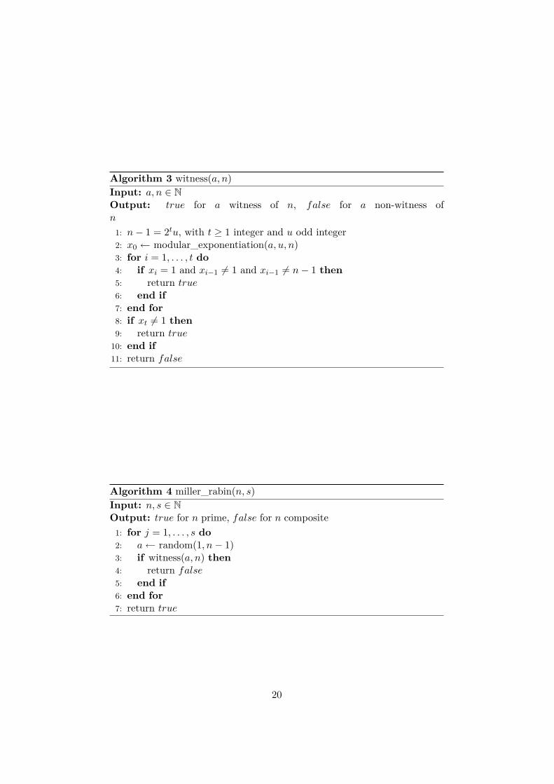
Algorithm 3 witness(a, n)Input: a, n ∈ NOutput: true for a witness of n, false for a non-witness ofn

1: n− 1 = 2tu, with t ≥ 1 integer and u odd integer2: x0 ← modular_exponentiation(a, u, n)3: for i = 1, . . . , t do

4: if xi = 1 and xi−1 �= 1 and xi−1 �= n− 1 then


7: end for

8: if xt �= 1 then


11: return false

Algorithm 4 miller_rabin(n, s)Input: n, s ∈ NOutput: true for n prime, false for n composite

1: for j = 1, . . . , s do

2: a← random(1, n− 1)3: if witness(a, n) then


6: end for

7: return true

20

n if an−1 �≡ 1 (mod n) (so this implies that n is composite). The followingtheorem tells us something important.

Theorem 4.17

If n is an odd composite number, the number of witnesses of n is at leastn−1

2 .

Proof. We have shown in theorem 4.16 that the set (called S) of non-witnesses of n for the Miller-Rabin algorithm is contained in a proper sub-group of Z∗n, called B. By the Lagrange theorem, we know that the order of asubgroup divides the order of the group. So |B| divides |Z∗n| = φ(n) ≤ n−1.So, since S ⊆ B, we have |S| ≤ |B| ≤ |Z

∗n|2 ≤

n−12 . This means that the

number of non-witnesses is at most n−12 . So the number of witnesses is at

least n−12 .

So each time that we test the witness function, we have the probabilityof at least 1

2 to obtain true. So we have the following theorem (stated withoutproof).

Theorem 4.18

For every odd integer n > 2 and every positive integer s (number of randomnumbers tested if they are witnesses or not), the probability of error of theMiller-Rabin algorithm is at most 2−s.

In practice, we can run the algorithm for s = 50 to have a good proba-bility that if n is composite we catch a witness.

21

5 The Fermat algorithm

The Fermat algorithm is based on the same principles as the Miller-Rabinalgorithm, so uses the Fermat’s little theorem as principal criterion. But itis less restrictive because it does not check the square roots when doing thecalculus. Its criterion is the one in 4.7.

5.1 General idea

The Fermat algorithm is exactly the same algorithm as the Miller-Rabinalgorithm, except for the checking of square root of 1 (mod n).

5.2 More precisely

Let n ∈ N be the input of our algorithm. We want to know if n is prime orcomposite.The Fermat algorithm is composed by exactly the same functions as theMiller-Rabin algorithm:

1. the witness function;


3. the miller_rabin function.

The only thing that changes is the witness function. It does not usethe corollary 4.14, but only bases its criterion on the Fermat’s little theorem(theorem 4.6).The witness function in this algorithm tells us if a is a "witness" that n iscomposite or not (with the criterion of Fermat’s little theorem).We calculate an−1 (mod n) with the modular_exponentiation function.If an−1 �≡ 1 (mod n), then the function says that n is composite (becauseof the contraposition of Fermat’s little theorem).If we’re not in this case, the function says that n is prime.

Here follows the pseudocode of the witness function for the Fermatalgorithm.

5.3 Running time

Since this algorithm is quite the same as the Miller-Rabin algorithm (itonly checks less things, but performs the same calculations), it has the samerunning time as the Miller-Rabin algorithm.

22

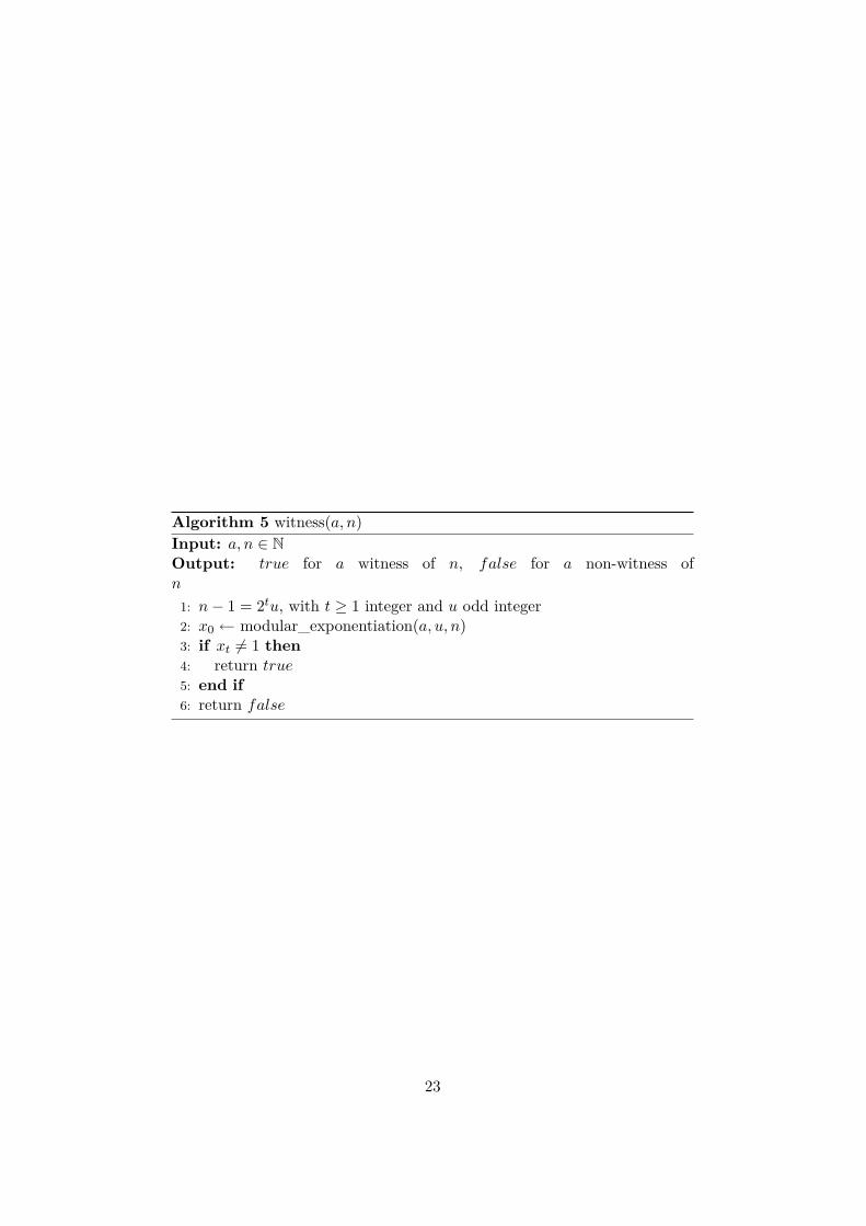
Algorithm 5 witness(a, n)Input: a, n ∈ NOutput: true for a witness of n, false for a non-witness ofn

1: n− 1 = 2tu, with t ≥ 1 integer and u odd integer2: x0 ← modular_exponentiation(a, u, n)3: if xt �= 1 then


6: return false

23

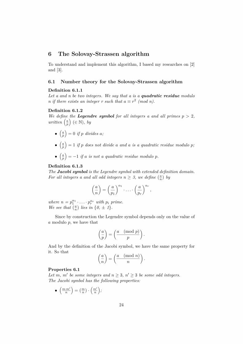
6 The Solovay-Strassen algorithm

To understand and implement this algorithm, I based my researches on [2]and [3].

6.1 Number theory for the Solovay-Strassen algorithm

Definition 6.1.1

Let a and n be two integers. We say that a is a quadratic residue modulon if there exists an integer r such that a ≡ r2 (mod n).

Definition 6.1.2

We define the Legendre symbol for all integers a and all primes p > 2,written

�ap

�(∈ N), by

•�ap

�= 0 if p divides a;

•�ap

�= 1 if p does not divide a and a is a quadratic residue modulo p;

•�ap

�= −1 if a is not a quadratic residue modulo p.

Definition 6.1.3

The Jacobi symbol is the Legendre symbol with extended definition domain.For all integers a and all odd integers n ≥ 3, we define

� an

�by

�a

n

�=�a

p1

�α1· . . . ·

�a

pr

�αr,

where n = pα11 · . . . · pαrr with pi prime.

We see that� an

�lies in {0, ± 1}.

Since by construction the Legendre symbol depends only on the value ofa modulo p, we have that

�a

p

�=�a (mod p)

p

�.

And by the definition of the Jacobi symbol, we have the same property forit. So that �

a

n

�=�a (mod n)

n

�.

Properties 6.1

Let m, m� be some integers and n ≥ 3, n� ≥ 3 be some odd integers.The Jacobi symbol has the following properties:

•�m·m�n

�=�mn

�·�m�

n

�;

24

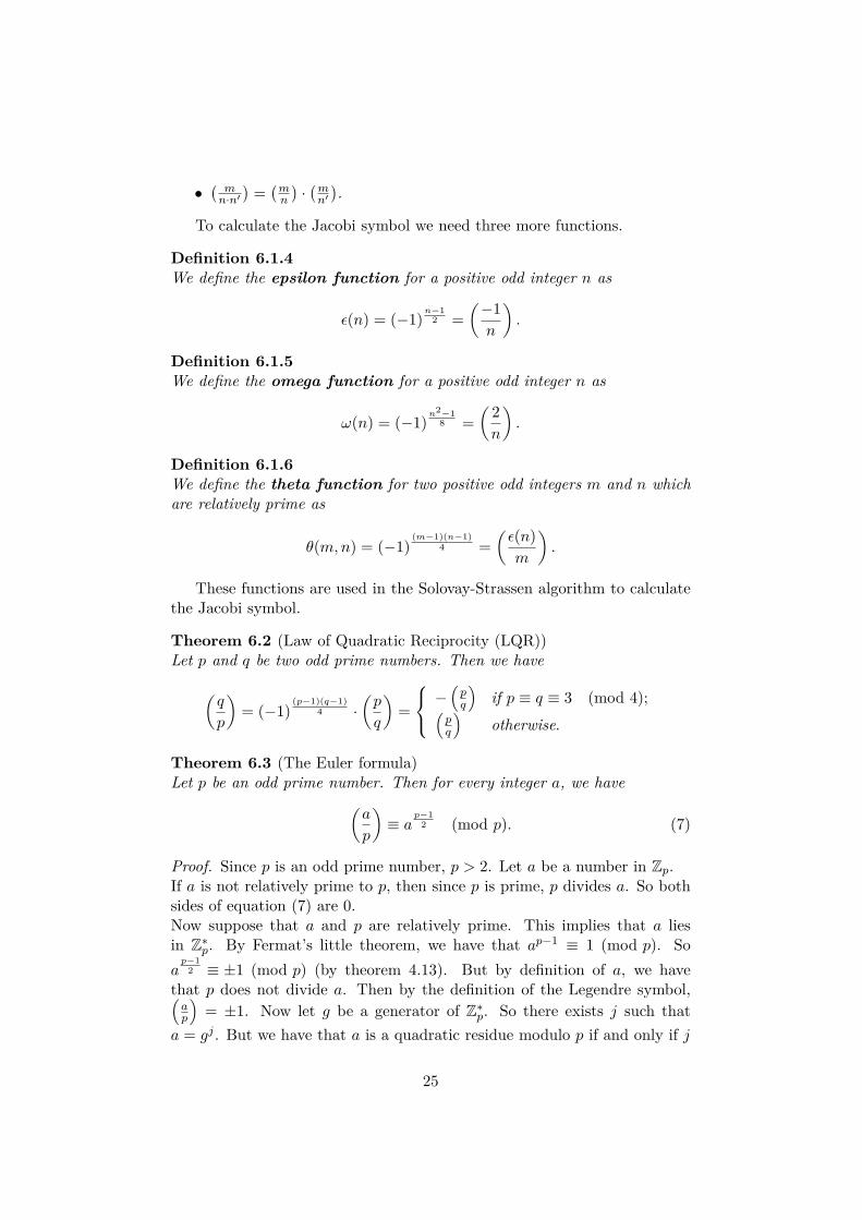
•� mn·n��

=�mn

�·�mn��.

To calculate the Jacobi symbol we need three more functions.

Definition 6.1.4

We define the epsilon function for a positive odd integer n as

�(n) = (−1)n−1

2 =�−1n

�.

Definition 6.1.5

We define the omega function for a positive odd integer n as

ω(n) = (−1)n2−1

8 =� 2n

�.

Definition 6.1.6

We define the theta function for two positive odd integers m and n whichare relatively prime as

θ(m,n) = (−1)(m−1)(n−1)

4 =��(n)m

�.

These functions are used in the Solovay-Strassen algorithm to calculatethe Jacobi symbol.

Theorem 6.2 (Law of Quadratic Reciprocity (LQR))Let p and q be two odd prime numbers. Then we have

�q

p

�= (−1)

(p−1)(q−1)4 ·

�p

q

�=

−�pq

�if p ≡ q ≡ 3 (mod 4);

�pq

�otherwise.

Theorem 6.3 (The Euler formula)Let p be an odd prime number. Then for every integer a, we have

�a

p

�≡ a

p−12 (mod p). (7)

Proof. Since p is an odd prime number, p > 2. Let a be a number in Zp.If a is not relatively prime to p, then since p is prime, p divides a. So bothsides of equation (7) are 0.Now suppose that a and p are relatively prime. This implies that a liesin Z∗p. By Fermat’s little theorem, we have that ap−1 ≡ 1 (mod p). Soap−1

2 ≡ ±1 (mod p) (by theorem 4.13). But by definition of a, we havethat p does not divide a. Then by the definition of the Legendre symbol,�ap

�= ±1. Now let g be a generator of Z∗p. So there exists j such that

a = gj . But we have that a is a quadratic residue modulo p if and only if j

25

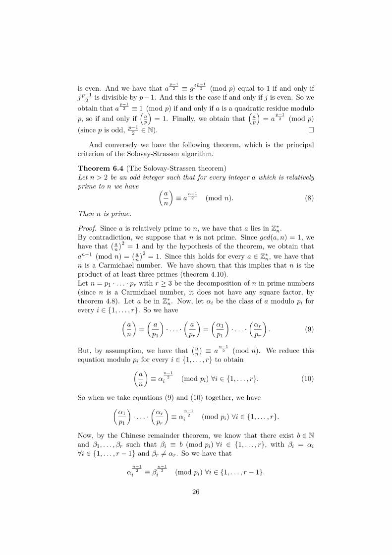
is even. And we have that ap−1

2 ≡ gjp−1

2 (mod p) equal to 1 if and only ifjp−1

2 is divisible by p−1. And this is the case if and only if j is even. So weobtain that a

p−12 ≡ 1 (mod p) if and only if a is a quadratic residue modulo

p, so if and only if�ap

�= 1. Finally, we obtain that

�ap

�= a

p−12 (mod p)

(since p is odd, p−12 ∈ N).

And conversely we have the following theorem, which is the principalcriterion of the Solovay-Strassen algorithm.

Theorem 6.4 (The Solovay-Strassen theorem)Let n > 2 be an odd integer such that for every integer a which is relativelyprime to n we have �

a

n

�≡ a

n−12 (mod n). (8)

Then n is prime.

Proof. Since a is relatively prime to n, we have that a lies in Z∗n.By contradiction, we suppose that n is not prime. Since gcd(a, n) = 1, wehave that

� an

�2 = 1 and by the hypothesis of the theorem, we obtain thatan−1 (mod n) =

� an

�2 = 1. Since this holds for every a ∈ Z∗n, we have thatn is a Carmichael number. We have shown that this implies that n is theproduct of at least three primes (theorem 4.10).Let n = p1 · . . . · pr with r ≥ 3 be the decomposition of n in prime numbers(since n is a Carmichael number, it does not have any square factor, bytheorem 4.8). Let a be in Z∗n. Now, let αi be the class of a modulo pi forevery i ∈ {1, . . . , r}. So we have

�a

n

�=�a

p1

�· . . . ·

�a

pr

�=�α1p1

�· . . . ·

�αr

pr

�. (9)

But, by assumption, we have that� an

�≡ a

n−12 (mod n). We reduce this

equation modulo pi for every i ∈ {1, . . . , r} to obtain�a

n

�≡ α

n−12i (mod pi) ∀i ∈ {1, . . . , r}. (10)

So when we take equations (9) and (10) together, we have�α1p1

�· . . . ·

�αr

pr

�≡ α

n−12i (mod pi) ∀i ∈ {1, . . . , r}.

Now, by the Chinese remainder theorem, we know that there exist b ∈ Nand β1, . . . ,βr such that βi ≡ b (mod pi) ∀i ∈ {1, . . . , r}, with βi = αi∀i ∈ {1, . . . , r − 1} and βr �= αr. So we have that

α

n−12i ≡ β

n−12i (mod pi) ∀i ∈ {1, . . . , r − 1}.

26

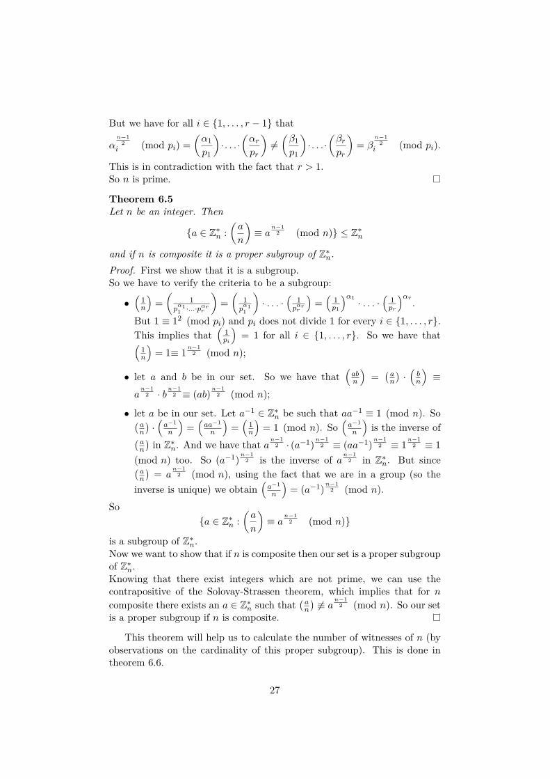
But we have for all i ∈ {1, . . . , r − 1} that

α

n−12i (mod pi) =

�α1p1

�· . . . ·�αr

pr

��=�β1p1

�· . . . ·�βr

pr

�= β

n−12i (mod pi).

This is in contradiction with the fact that r > 1.So n is prime.

Theorem 6.5

Let n be an integer. Then

{a ∈ Z∗n :�a

n

�≡ a

n−12 (mod n)} ≤ Z∗n

and if n is composite it is a proper subgroup of Z∗n.Proof. First we show that it is a subgroup.So we have to verify the criteria to be a subgroup:

•�

1n

�=�

1pα11 ·...·p

αrr

�=�

1pα11

�· . . . ·

�1pαrr

�=�

1p1

�α1 · . . . ·�

1pr

�αr .

But 1 ≡ 12 (mod pi) and pi does not divide 1 for every i ∈ {1, . . . , r}.This implies that

�1pi

�= 1 for all i ∈ {1, . . . , r}. So we have that

�1n

�= 1≡ 1

n−12 (mod n);

• let a and b be in our set. So we have that�abn

�=� an

�·�bn

�≡

an−1

2 · bn−1

2 ≡ (ab)n−1

2 (mod n);

• let a be in our set. Let a−1 ∈ Z∗n be such that aa−1 ≡ 1 (mod n). So� an

�·�a−1n

�=�aa−1n

�=�

1n

�= 1 (mod n). So

�a−1n

�is the inverse of

� an

�in Z∗n. And we have that a

n−12 · (a−1)

n−12 ≡ (aa−1)

n−12 ≡ 1

n−12 ≡ 1

(mod n) too. So (a−1)n−1

2 is the inverse of an−1

2 in Z∗n. But since� an

�= a

n−12 (mod n), using the fact that we are in a group (so the

inverse is unique) we obtain�a−1n

�= (a−1)

n−12 (mod n).

So{a ∈ Z∗n :

�a

n

�≡ a

n−12 (mod n)}

is a subgroup of Z∗n.Now we want to show that if n is composite then our set is a proper subgroupof Z∗n.Knowing that there exist integers which are not prime, we can use thecontrapositive of the Solovay-Strassen theorem, which implies that for ncomposite there exists an a ∈ Z∗n such that

� an

��≡ a

n−12 (mod n). So our set

is a proper subgroup if n is composite.

This theorem will help us to calculate the number of witnesses of n (byobservations on the cardinality of this proper subgroup). This is done intheorem 6.6.

27

6.2 General idea

Recall Solovay-Strassen theorem (theorem 6.4). It says that if n > 2 isan odd integer such that for every integer a which is relatively prime ton we have

� an

�≡ a

n−12 (mod n), then n is prime. So the Solovay-Strassen

algorithm checks equation (8) for some a ∈ Z∗n. If it finds an a such thatthis equation is not verified, then it declares that n is composite. And if,for a large number of such a (their number, s ∈ N, is chosen by the user),equation (8) is verified, the Solovay-Strassen algorithm declares that n isprime. These numbers a are randomly chosen in {1, . . . , n}.

6.3 More precisely

Let n ∈ N be the input of our algorithm. We want to know if n is prime orcomposite.The Solovay-Strassen algorithm uses a random function that gives it a ran-dom number a ∈ Z∗n. This algorithm is composite by three principal func-tions:


2. the jacobi function;

3. the solovay_strassen function.

The modular_exponentiation function is the same as in the Miller-Rabin algorithm. It is used to calculate a

n−12 (mod n).

The jacobi function calculates the Jacobi symbol. We want to calculate�uv

�for an integer u and an odd integer v ≥ 3. The principal steps of this

calculation are the following:Let t ≥ 0 be an integer and r be an odd integer such that u = 2tr. So wehave

�u

v

�=�

2trv

�

=�

2tv

�

·�r

v

�.

The second equation is obtained by applying the properties of the Jacobisymbol. But we know that

�2tv

�= ±1 because v is odd and 2 (and so 2t)

28

does not divide v. And then we can apply the LQR. We have then�

2tv

�

·�r

v

�= ±

�r

v

�

= ±�v

r

�

= ±�s

r

�,

where s is an integer such that v = k · r + s for some integer k.We now set s =

�pαii with αi integers, pi primes and pi �= pj for all i �= j.

So

±�s

r

�= ±

��pαii

r

�

= ±��pi

r

�αi.

Again, the second equality is obtained by using the properties of the Jacobisymbol.If one of the pi is equal to 2, then we have

�2r

�αi = ±1. So we can assumethat none of the pj remaining are equal to 2. We can use again the LQR tohave

±��pi

r

�αi= ±

�� rpi

�αi.

There are now only Legendre symbols and we can calculate them directly(using the definition of Legendre symbol). And the function returns thecalcuated value of

�uv

�.

The solovay_strassen function tests if the jacobi function of a and nis equal to the modular_exponentiation function of a and n (with expo-nent n−1

2 ). If the answer at this question is no, then the solovay_strassen

function says that n is composite. If not, then it declares that n is prime.

The following pseudocodes are the ones of the jacobi function and thesolovay_strassen function.

Recall that �(·), ω(·) and θ(·) are the functions defined in 6.1.4, 6.1.5and 6.1.6.

6.4 Running time

The cost of the computation of the jacobi symbol as described above (inthe jacobi function) is O(len(n)2). The computation of the right partof the equation of the Solovay-Strassen theorem (which is done by the

29

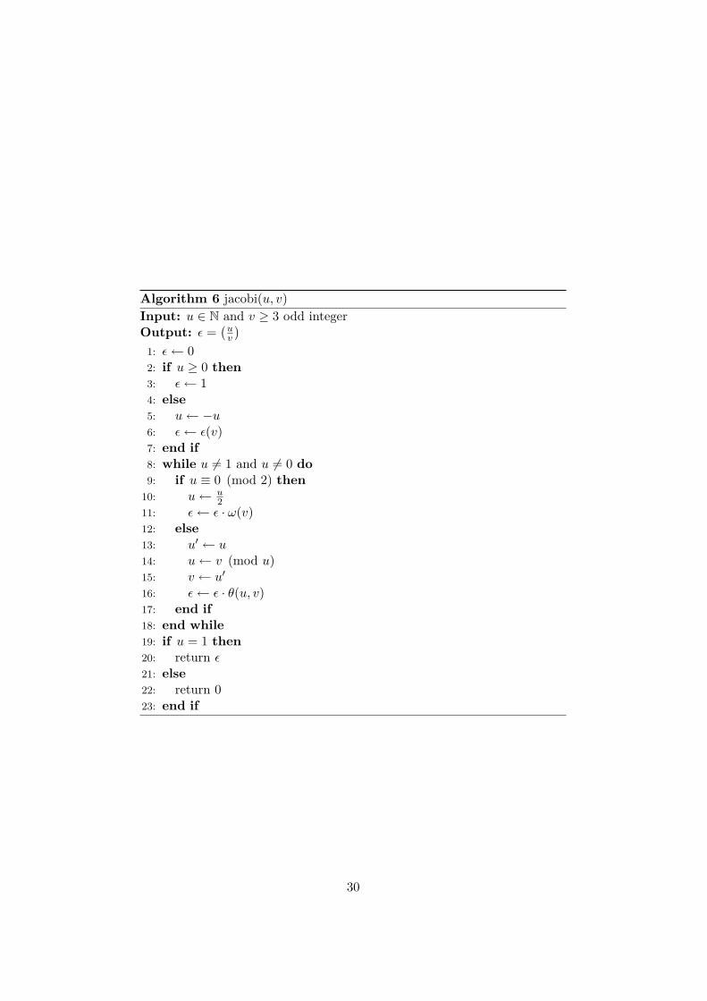
Algorithm 6 jacobi(u, v)Input: u ∈ N and v ≥ 3 odd integerOutput: � =

�uv

�

1: �← 02: if u ≥ 0 then

3: �← 14: else

5: u← −u6: �← �(v)7: end if

8: while u �= 1 and u �= 0 do

9: if u ≡ 0 (mod 2) then

10: u← u2

11: �← � · ω(v)12: else

13: u� ← u14: u← v (mod u)15: v ← u�16: �← � · θ(u, v)17: end if

18: end while

19: if u = 1 then

20: return �21: else

22: return 023: end if

30

Algorithm 7 solovay_strassen(n, s)Input: n, s ∈ NOutput: true for n prime, false for n composite

1: for j = 1, . . . , s do

2: a = random(1,n-1)3: if n = 2 then

4: return true5: else

6: if n ≡ 0 (mod 2) then


9: end if

10: if jacobi(a, n) �= modular_exponentiation(a, n) then


13: end for

14: return true

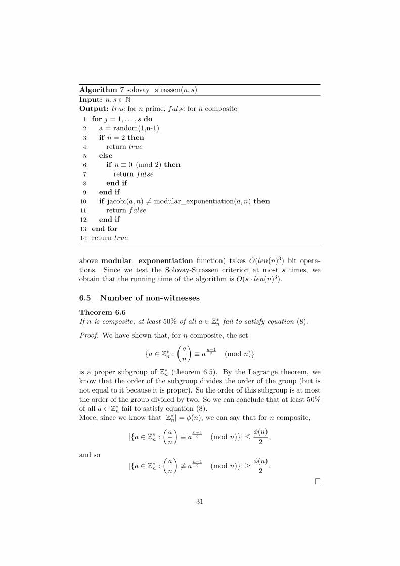
above modular_exponentiation function) takes O(len(n)3) bit opera-tions. Since we test the Solovay-Strassen criterion at most s times, weobtain that the running time of the algorithm is O(s · len(n)3).

6.5 Number of non-witnesses

Theorem 6.6

If n is composite, at least 50% of all a ∈ Z∗n fail to satisfy equation (8).

Proof. We have shown that, for n composite, the set

{a ∈ Z∗n :�a

n

�≡ a

n−12 (mod n)}

is a proper subgroup of Z∗n (theorem 6.5). By the Lagrange theorem, weknow that the order of the subgroup divides the order of the group (but isnot equal to it because it is proper). So the order of this subgroup is at mostthe order of the group divided by two. So we can conclude that at least 50%of all a ∈ Z∗n fail to satisfy equation (8).More, since we know that |Z∗n| = φ(n), we can say that for n composite,

|{a ∈ Z∗n :�a

n

�≡ a

n−12 (mod n)}| ≤ φ(n)2 ,

and so|{a ∈ Z∗n :

�a

n

��≡ a

n−12 (mod n)}| ≥ φ(n)2 .

31

So if n is composite, then we will have to try equation (8) for a certainnumber of a before finding a witness of the fact that n is composite. It canbe observed that this quantity of non-witnesses can depend on the form ofn (by exemple: if n is the product of two primes, if n is the product of twoGermain primes, ...).

32

7 The AKS algorithm

To understand this algorithm (AKS stands for Agrawal, Kayal and Saxena,who founds this algorithm), I based my researches on [4].

Since the last few years, there was no known deterministic polynomial-time algorithm of finding if an integer is prime or not. But the 6 August2002, Agrawal, Kayal and Saxena, three indian mathematicians, found suchan algorithm. This algorithm is called AKS (for the names of the people whofound it) and is presented in the following section. The importance of thisalgorithm is more theoretical than practical, the probabilistic algorithms,such as the Miller-Rabin algorithm seen before, being much more efficient.

7.1 Number theory for the AKS algorithm

Definition 7.1.1

Let R be a ring. An R-algebra is a ring E with a ring homomorphismτ : R→ E.

In our case, we are interested in this definition for K[X] in the place ofE and the homomorphism τ which sends a ∈ R to the constant polynomiala ∈ K[X].

Definition 7.1.2

Let E and E� be some R-algebras with associated maps τ : R → E andτ � : R → E�. We call ρ : E → E� a R-algebra homomorphism if andonly if ρ is a ring homomorphism from E to E� and ρ(τ(a)) = τ �(a) for alla ∈ R.

The AKS algorithm bases his criterion on principally one theorem, whichis the following.

Theorem 7.1

Let n > 1 be an integer.If n is prime, then

(X + a)n ≡ Xn + a (mod n) (11)

for every a ∈ Zn, where X is an indefinite of Zn.If n is composite, then

(X + a)n �≡ Xn + a (mod n)

for every a ∈ Z∗n, where X is an indefinite of Zn.But this criterion is not efficient because only evaluating the left-hand

side of equation (11) already takes time O(n) which is not polynomial inlen(n). The AKS algorithm uses another more restrictive criterion, whichis to test this equation modulo Xr − 1 instead of modulo n for a suitablevalue of r.

33

Theorem 7.2

If (X + a)n ≡ Xn + a (mod Xr − 1) holds in Zn[X] for a certain r and acertain number of a, then n is prime.

The r and the number of a necessary to have this result is explained inthe algorithm below.

7.2 The algorithm

Let n ∈ N be the input of our algorithm. We want to know if n is prime orcomposite. The AKS algorithm is as follow:

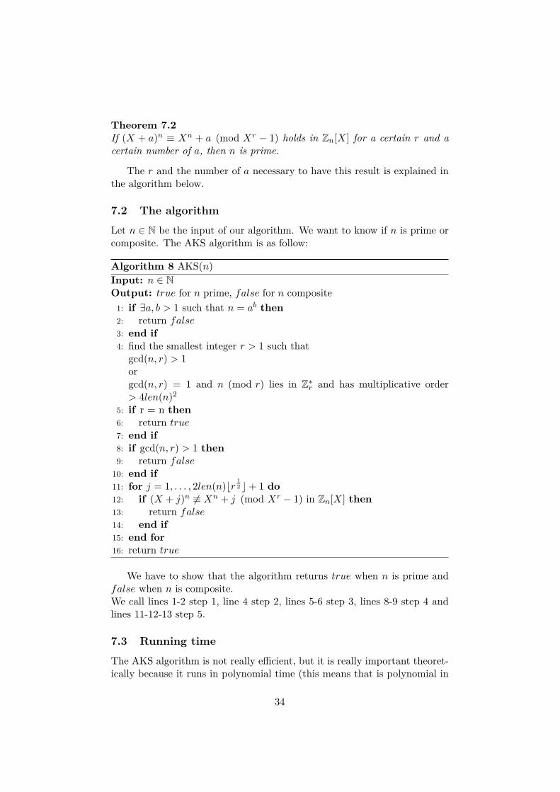
Algorithm 8 AKS(n)Input: n ∈ NOutput: true for n prime, false for n composite

1: if ∃a, b > 1 such that n = ab then


4: find the smallest integer r > 1 such thatgcd(n, r) > 1orgcd(n, r) = 1 and n (mod r) lies in Z∗r and has multiplicative order> 4len(n)2

5: if r = n then


8: if gcd(n, r) > 1 then


11: for j = 1, . . . , 2len(n)�r 12 �+ 1 do

12: if (X + j)n �≡ Xn + j (mod Xr − 1) in Zn[X] then


15: end for

16: return true

We have to show that the algorithm returns true when n is prime andfalse when n is composite.We call lines 1-2 step 1, line 4 step 2, lines 5-6 step 3, lines 8-9 step 4 andlines 11-12-13 step 5.

7.3 Running time

The AKS algorithm is not really efficient, but it is really important theoret-ically because it runs in polynomial time (this means that is polynomial in

34

len(n)).We show that analyzing each step of the algorithm.

• For step 1, there already exists an algorithm of perfect power testingwhich runs in O(len(n)3len(len(n))), which is polynomial in len(n).

• For step 2, the search of r can be done by brute-force. The compu-tation of gcd(n, r) can be done using Euclid’s algorithm which runsin O(len(n)2). If r does not divide n and the multiplicative order ofn (mod r) in Z∗r is greater than m = 4len(n)2, then it can be shownthat the least r verifying these hypothesis is O(m2len(n)). The deter-mination of the multiplicative order of n (mod r) in Z∗r can be doneby brute-force, using modular exponentiation to compute successivepowers of n modulo r, which runs in polynomial time. So r found instep 2 is at most O(len(n)5).

• For step 3 and 4, which are only tests, we easily see that they are inpolynomial time.

• For step 5, we see that we have to perform O(r 12 len(n)) exponenti-

ations (one for each iteration). To perform the exponentiation, weuse the modular_exponentiation function which costs O(len(n))for the len(n) successive squaring steps, O(r2) for the multiplicationof two polynomials of degree at most r − 1 in each squaring step andO(len(n)2) for the cost of one operation in Zn. So the step 5 runs inO(r 5

2 len(n)4).

Put together, since the r found in step 2 is in O(len(n)5), this implies thatthe AKS algorithm runs in O(len(n) 33

2 ).

7.4 Correctness

The proof of the correctness being rather long, this is only the idea of themain steps of the proof of the correctness of the AKS algorithm.

First, we show that if n is prime, then the algorithm outputs true.We clearly see that the test in step 1 will fail. If the algorithm does notreturn true in step 3, then the test in step 4 will fail too (because of theprimality of n). Because of theorem 7.1, the test in step 5 will fail for everyj. So the output will be true.

Now we show that if n is composite, then the algorithm outputs false.If n is a prime power, it will be detected in the first step. So we can assumethat n is not a perfect power. Assume that a suitable value has been foundin step 2. So the test in step 3 will certainly fail. If the test in step 4 passes,we are done, so we assume that it fails. We can now assume that all prime

35

factors of n are greater than r (if not we would have taken another value ofr in step 2). We have to show that one of the tests in step 5 will pass. Wewill do this by contradiction. We suppose that every test fails and derive acontradiction.For the rest of the proof, we fix a prime divisor p of n. Since p divides n,we have a natural ring homomorphism from Zn[X] to Zp[X]. This impliesthat if the congruence in step 5 holds in Zn[X], then it will hold in Zp[X]too. So for the rest of the proof we will work in Zp[X].Here is a summary of the assumptions we make:

1. n > 1, r > 1, and l ≥ 1 are integers, p is a prime dividing n, andgcd(n, r) = 1;

2. n is not a prime power;

3. p > r;

4. the congruence

(X + j)n ≡ Xn + j (mod Xr − 1)

holds for j = 1, . . . , l in Zp[X];

5. the multiplicative order of n (mod r) in Z∗r is greater than 4len(n)2;

6. l > 2len(n)�r 12 �.

From now on, only assumption 1 will always be in force. The other assump-tions will be explicitly named when they are necessary.The goal now is to show that assumptions 1, 2, 3, 4, 5 and 6 cannot all betrue simultaneously.First, we define E = Zp[X]/(Xr − 1) and ξ = X (mod Xr − 1) ∈ E. So wehave that

E = Zp[ξ].

And this implies that every element of E can be uniquely expressed asg(ξ) = g (mod Xr − 1) for some g ∈ Zp[X] of degree less than r. Thesedefinitions mean that we have g(ξ) = 0 for an arbitrary g ∈ Zp[X] if andonly if Xr− 1 divides g. We can easily see that ξ has multiplicative order r.We define now the following function for all integers k:

σk : E → E, g(ξ) �→ g(ξk),

with g an arbitrary element of Zp[X]. Now, for k ∈ Z∗r , let’s define thefollowing function: σk : Zp[X] → E, g �→ g(ξk), which is the polynomialevaluation map. Note that, by assumption 1, n and p lie in Z∗r . By showingthat the kernel of σk is (Xr − 1) and the image of σk is E, we show that σkis a ring automorphism. So for all k, k� ∈ Z∗r we obtain that:

36

• σk = σk� if and only if ξk = ξk� if and only if k = k� (mod r);

• σk ◦ σk� = σk� ◦ σk = σkk� .

Now, since E is of characteristic p and using Fermat’s little theorem (theorem4.6), we have that the p-power map is a Zp-algebra homomorphism. Letα ∈ E and its expression α = g(ξ) for some g ∈ Zp[X]. We obtain that

αp = g(ξ)p = g(ξp) = σp(α).

So we see that σp acts like the p-power map.We can rewrite assumption 4 as

σn(ξ + j) = (ξ + j)n for j = 1, . . . , l.

This would mean that for every n the map σn would act like the n-powermap on each element of the form ξ + j, which seems really strange andgives the intuition that we will derive a contradiction somewhere looking atelements of this form.We will now examine the elements and the values of n such that σn behaveslike the n-power map on these elements. To do so we define two sets:

C(α) = {k ∈ Z∗r : σk(α) = αk}

for α ∈ E andD(k) = {α ∈ E : σk(α) = αk}

for k ∈ Z∗r . So we see that C(α) is the set of values of k such that σk actslike the k-power map on α and D(k) is the set of values of α such that σkacts like the k-power map on α. We remark that 1 and p are in C(α) forall α ∈ E, α is in D(p) for all α ∈ E and 1 is in D(k) for all k ∈ Z∗r . Usingthe properties of σk, we can easily show that the sets C(α) and D(k) aremultiplicative.Now, let us define

• s as the multiplicative order of p (mod r) in Z∗r , and

• t as the order of the subgroup of Z∗r generated by p (mod r) and n(mod r).

In the following we will work a lot with elements of this subgroup.Let F be the extension field of degree s over Zp, which is the field with pselements. This implies that F ∗ is cyclic and has order ps − 1. By definitionof s, we have that r divides ps − 1. And this implies that there exists anelement ζ ∈ F ∗ of multiplicative order r.Let us now define the Zp-algebra homomorphism

τ : E → F , g(ξ) �→ g(ζ)

37

for g ∈ Zp[X] (this is well-defined because Xr − 1 is the kernel of theevaluation map that sends g ∈ Zp[X] to g(ζ) ∈ F ).We define now the set

S = τ(D(n)),

which is the set of the images under τ of all elements in E over which σn actslike the n-power map. We will observe this set and derive a contradictionfrom some observations on its cardinality.First, we have the following lemma.

Lemma 7.3

Under assumption 2, we have

|S| ≤ n2�t12 �.

Proof. To do that we consider the set

I = {nupv : u, v = 0, . . . , �t12 �}.

Noting that n is not a prime power (by assumption 2), we can easily seethat for each distinct pair (u, v) we obtain a distinct value of nupv. Sinceu and v each take �t 12 � + 1 values, there are strictly more than t distinctvalues of nupv. So |I| > t. But recall that t = |�p (mod r), n (mod r)�|. Sothis means that there exist some k and k� in I which are distinct but equalmodulo r. Since k and k� lie in I, we have that they both are less thann2�t

12 �.

Now, let α ∈ D(n). This implies that n ∈ C(α). Since 1 ∈ C(α) andp ∈ C(α), we have that for every u and v non negative integers nupv ∈ C(α).So k, k� ∈ C(α). This means that σk(α) = αk and σk�(α) = αk� . But sincek ≡ k� (mod r), we have σk = σk� , which implies that αk = αk� . Weapply τ to this and use the fact that it is an homomorphism to obtainτ(α)k = τ(α)k� . So τ(α) is a root of the polynomial Xk −Xk� (which is anon-zero polynomial since k �= k�). Since this holds for every α ∈ D(n), everyelement of S is a root of Xk−Xk� . This polynomial being of degree at mostmax{k, k�} ≤ n2�t

12 �, we have that |S| ≤ |{roots of Xk−Xk�}| ≤ n2�t

12 �.

Now we limit the other side of |S|.

Lemma 7.4

Under assumptions 3 and 4, we have

|S| ≥ 2min(t,l) − 1.

Proof. To simplify the notations, we write m = min(t, l) (remember thatt = |�p (mod r), n (mod r)�| and l is the number of values of j we test instep 5 of the algorithm). We see that assumption 4 implies that ξ+j ∈ D(n)

38

for j = 1, . . . ,m. But assumption 3 means that p > r and by definition oft, we have r > t and by definition of m, we have t ≥ m. So we havep > r > t ≥ m. This implies that the integers j = 1, . . . ,m are distinctmodulo p. So we can see that D(n) is very large if we take t and l large andwe will see that nothing "collapses" under τ .To obtain the 2m − 1, we have to work on a set which is the following:

P =

m�

j=1(X + j)ej ∈ Zp[X] : ej ∈ {0, 1} for j = 1, . . . ,m and

m�

j=1ej < m

.

Since all j are distinct modulo p, there exists a bijection between the setP and the different choices of the ej for j = 1, . . . ,m (with the condition

thatm�

j=1ej < m). So we have that |P | = 2m − 1. We define now two sets:

P (ξ) = {f(ξ) ∈ E : f ∈ P} and P (ζ) = {f(ζ) ∈ F : f ∈ P}, which isclearly the image of P (ξ) under τ . Since ξ + j ∈ D(n) for j = 1, . . . ,mand D(n) is multiplicative, we have that P (ξ) ⊆ D(n). So we have thatP (ζ) = τ(P (ξ)) ⊆ τ(D(n)) = S, hence |P (ζ)| ≤ |S|. So it suffices to showthat |P (ζ)| = 2m − 1 (since |P | = 2m − 1, it will not be more). We do thisby contradiction.We suppose that |P (ζ)| < 2m− 1. This implies that there exist two distinctpolynomials g, h ∈ P such that g(ζ) = h(ζ). Since g, h ∈ P , we havethat g and h are both of degree at most t − 1 (more precisely at mostm− 1), that g(ξ), h(ξ) ∈ D(n) and that τ(g(ξ)) = τ(h(ξ)). So we have that1, p, n ∈ C(g(ξ)) and 1, p, n ∈ C(h(ξ)). Hence for all k of the form nupv foru and v non-negative integers, k ∈ C(g(ξ)) and k ∈ C(h(ξ)). So we obtainthat, since τ(g(ξ)) = τ(h(ξ)), τ(g(ξ))k = τ(h(ξ))k. Hence, using that τ isan homomorphism, we have

0 = τ(g(ξ))k − τ(h(ξ))k

= τ(g(ξ)k)− τ(h(ξ)k)= τ(g(ξk))− τ(h(ξk))= g(ζk)− h(ζk).

So we have obtained a non-zero polynomial f = g − h ∈ Zp[X] which hasζk ∈ F as root for all k of the form nupv. Recall that ζ has multiplicativeorder r. So ζk = ζk� if and only if k ≡ k� (mod r). But we have shown thatthere are exactly t distinct values for an integer k of the form nupv (mod r).So there are exactly t different values of ζk in F , which are all roots of f .But f is of degree at most t− 1, so it can only have t− 1 roots, which is acontradiction. So |P (ζ)| has to be equal to 2m − 1.

So we have shown that under assumptions 2, 3 and 4, we have

2min(t,l) − 1 ≤ |S| ≤ n2�t12 �.

39

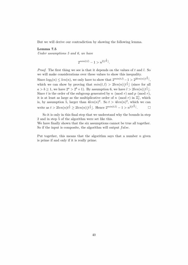
But we will derive our contradiction by showing the following lemma.

Lemma 7.5

Under assumptions 5 and 6, we have

2min(t,l) − 1 > n2�t12 �.

Proof. The first thing we see is that it depends on the values of t and l. Sowe will make considerations over these values to show this inequality.Since log2(n) ≤ len(n), we only have to show that 2min(t,l)−1 > 22len(n)�t

12 �,

which we can show by proving that min(t, l) > 2len(n)�t 12 � (since for alla > b ≥ 1, we have 2a > 2b+ 1). By assumption 6, we have l > 2len(n)�t 12 �.Since t is the order of the subgroup generated by n (mod r) and p (mod r),it is at least as large as the multiplicative order of n (mod r) in Z∗r , whichis, by assumption 5, larger than 4len(n)2. So t > 4len(n)2, which we canwrite as t > 2len(n)t 12 ≥ 2len(n)�t 12 �. Hence 2min(t,l) − 1 > n2�t

12 �.

So it is only in this final step that we understand why the bounds in step2 and in step 5 of the algorithm were set like this.We have finally shown that the six assumptions cannot be true all together.So if the input is composite, the algorithm will output false.

Put together, this means that the algorithm says that a number n givenis prime if and only if it is really prime.

40

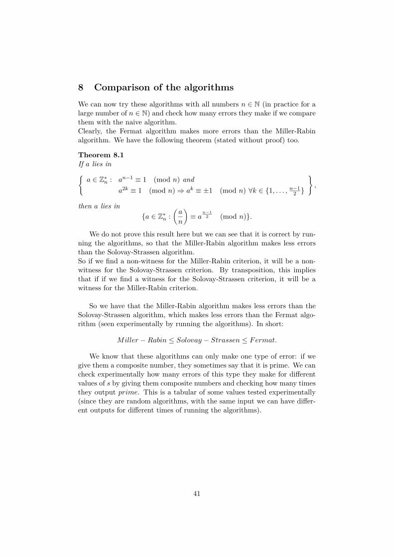
8 Comparison of the algorithms

We can now try these algorithms with all numbers n ∈ N (in practice for alarge number of n ∈ N) and check how many errors they make if we comparethem with the naive algorithm.Clearly, the Fermat algorithm makes more errors than the Miller-Rabinalgorithm. We have the following theorem (stated without proof) too.

Theorem 8.1

If a lies in�a ∈ Z∗n : an−1 ≡ 1 (mod n) and

a2k ≡ 1 (mod n)⇒ ak ≡ ±1 (mod n) ∀k ∈ {1, . . . , n−12 }

�

,

then a lies in{a ∈ Z∗n :

�a

n

�≡ a

n−12 (mod n)}.

We do not prove this result here but we can see that it is correct by run-ning the algorithms, so that the Miller-Rabin algorithm makes less errorsthan the Solovay-Strassen algorithm.So if we find a non-witness for the Miller-Rabin criterion, it will be a non-witness for the Solovay-Strassen criterion. By transposition, this impliesthat if if we find a witness for the Solovay-Strassen criterion, it will be awitness for the Miller-Rabin criterion.

So we have that the Miller-Rabin algorithm makes less errors than theSolovay-Strassen algorithm, which makes less errors than the Fermat algo-rithm (seen experimentally by running the algorithms). In short:

Miller −Rabin ≤ Solovay − Strassen ≤ Fermat.

We know that these algorithms can only make one type of error: if wegive them a composite number, they sometimes say that it is prime. We cancheck experimentally how many errors of this type they make for differentvalues of s by giving them composite numbers and checking how many timesthey output prime. This is a tabular of some values tested experimentally(since they are random algorithms, with the same input we can have differ-ent outputs for different times of running the algorithms).

41

Number of tested n: 220

1 ≤ n ≤ 220

s Fermat Miller-Rabin Solovay-Strassen2 465 347 3713 399 342 3505 377 339 341

10 349 339 33920 340 339 33950 339 339 339

This seems to be a lot of errors, but since 220 = 1048576, for s = 50,the algorithms make about 0.03% of errors. We see that increasing s in-creases the performance of the algorithms, but not as much as we wouldhave thought.


1 ≤ n ≤ 2100

s Fermat Miller-Rabin Solovay-Strassen2 0 0 03 0 0 05 0 0 0

10 0 0 020 0 0 050 0 0 0

We see that when we increase the size of the input, the algorithms makea lot less errors than in the previous example. This is probably becausesince the numbers are large they have more possible witnesses and so wehave more chance to find one.

Let n ∈ N composite number be the input of our algorithm. We can lookat how many random values we have to test before finding a witness of n.


1 ≤ n ≤ 220

s = 1 2 3 4Fermat 1022 2 0 0

Miller-Rabin 1024 0 0 0Solovay-Strassen 1023 1 0 0

We see that we find very quickly a witness of n. This shows that thealgorithms are efficient.But if we compare this result with the ones before, it seems strange to haveso many errors in the first example. Since this last example is more inagreement with the theory, there is probably an error in the implementation

42

of the algorithm for the first example.To have good examples we have to deal with big numbers and iterate ourfunctions many times. But it is difficult to make that on my own computer.This explain why these examples are so little.

43

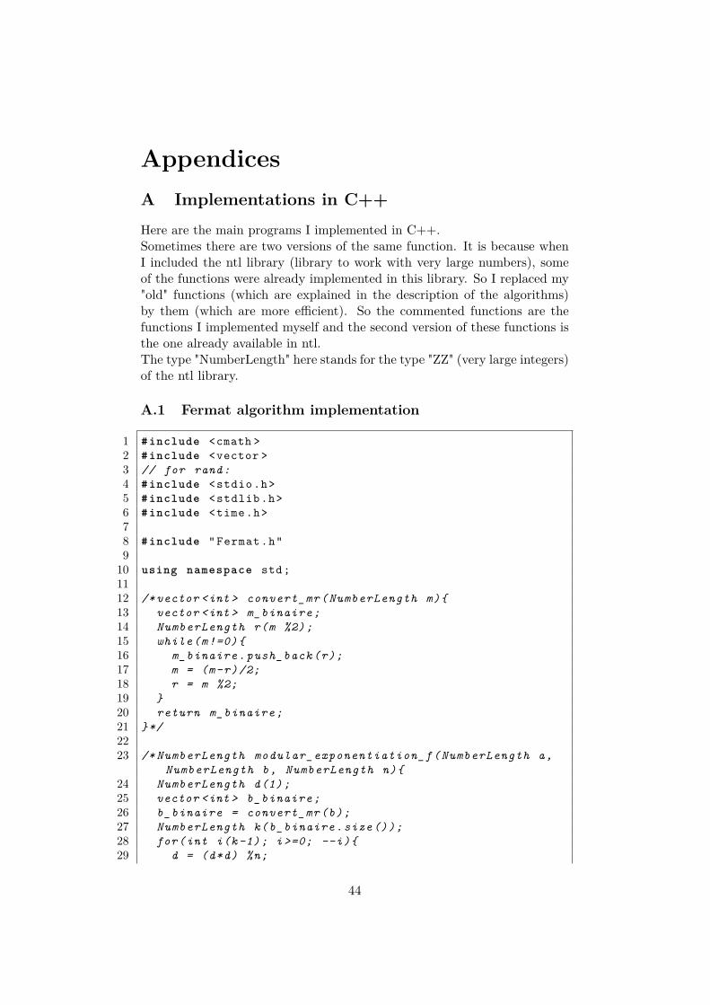
Appendices

A Implementations in C++

Here are the main programs I implemented in C++.Sometimes there are two versions of the same function. It is because whenI included the ntl library (library to work with very large numbers), someof the functions were already implemented in this library. So I replaced my"old" functions (which are explained in the description of the algorithms)by them (which are more efficient). So the commented functions are thefunctions I implemented myself and the second version of these functions isthe one already available in ntl.The type "NumberLength" here stands for the type "ZZ" (very large integers)of the ntl library.

A.1 Fermat algorithm implementation

1 # include <cmath >2 # include <vector >3 // for rand:4 # include <stdio.h>5 # include <stdlib .h>6 # include <time.h>78 # include " Fermat .h"9

10 using namespace std;1112 /* vector <int > convert_mr ( NumberLength m){13 vector <int > m_binaire ;14 NumberLength r(m %2);15 while(m!=0){16 m_binaire . push_back (r);17 m = (m-r)/2;18 r = m %2;19 }20 return m_binaire ;21 }*/2223 /* NumberLength modular_exponentiation_f ( NumberLength a,

NumberLength b, NumberLength n){24 NumberLength d(1);25 vector <int > b_binaire ;26 b_binaire = convert_mr (b);27 NumberLength k( b_binaire .size ());28 for(int i(k -1); i >=0; --i){29 d = (d*d) %n;

44

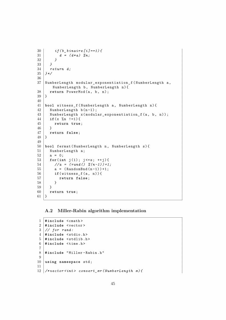
30 if( b_binaire [i ]==1){31 d = (d*a) %n;32 }33 }34 return d;35 }*/3637 NumberLength modular_exponentiation_f ( NumberLength a,

NumberLength b, NumberLength n){38 return PowerMod (a, b, n);39 }4041 bool witness_f ( NumberLength a, NumberLength n){42 NumberLength b(n -1);43 NumberLength x( modular_exponentiation_f (a, b, n));44 if(x %n !=1){45 return true;46 }47 return false;48 }4950 bool fermat ( NumberLength n, NumberLength s){51 NumberLength a;52 a = 0;53 for(int j(1); j<=s; ++j){54 //a = (rand () %(n -1))+1;55 a = ( RandomBnd (n -1))+1;56 if( witness_f (a, n)){57 return false;58 }59 }60 return true;61 }

A.2 Miller-Rabin algorithm implementation

1 # include <cmath >2 # include <vector >3 // for rand:4 # include <stdio.h>5 # include <stdlib .h>6 # include <time.h>78 # include "Miller -Rabin.h"9

10 using namespace std;1112 /* vector <int > convert_mr ( NumberLength m){

45

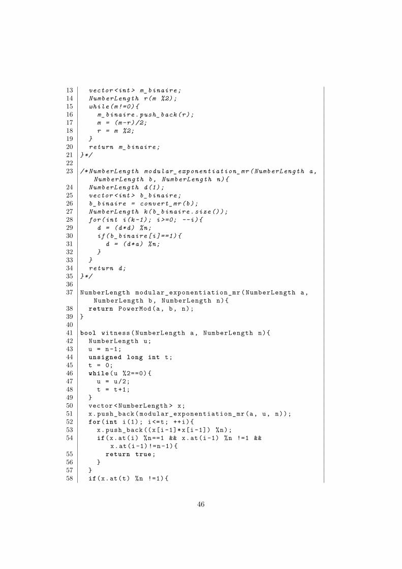
13 vector <int > m_binaire ;14 NumberLength r(m %2);15 while(m!=0){16 m_binaire . push_back (r);17 m = (m-r)/2;18 r = m %2;19 }20 return m_binaire ;21 }*/2223 /* NumberLength modular_exponentiation_mr ( NumberLength a,

NumberLength b, NumberLength n){24 NumberLength d(1);25 vector <int > b_binaire ;26 b_binaire = convert_mr (b);27 NumberLength k( b_binaire .size ());28 for(int i(k -1); i >=0; --i){29 d = (d*d) %n;30 if( b_binaire [i ]==1){31 d = (d*a) %n;32 }33 }34 return d;35 }*/3637 NumberLength modular_exponentiation_mr ( NumberLength a,

NumberLength b, NumberLength n){38 return PowerMod (a, b, n);39 }4041 bool witness ( NumberLength a, NumberLength n){42 NumberLength u;43 u = n -1;44 unsigned long int t;45 t = 0;46 while (u %2==0) {47 u = u/2;48 t = t+1;49 }50 vector < NumberLength > x;51 x. push_back ( modular_exponentiation_mr (a, u, n));52 for(int i(1); i<=t; ++i){53 x. push_back ((x[i -1]*x[i -1]) %n);54 if(x.at(i) %n==1 && x.at(i -1) %n !=1 &&

x.at(i -1) !=n -1){55 return true;56 }57 }58 if(x.at(t) %n !=1){

46

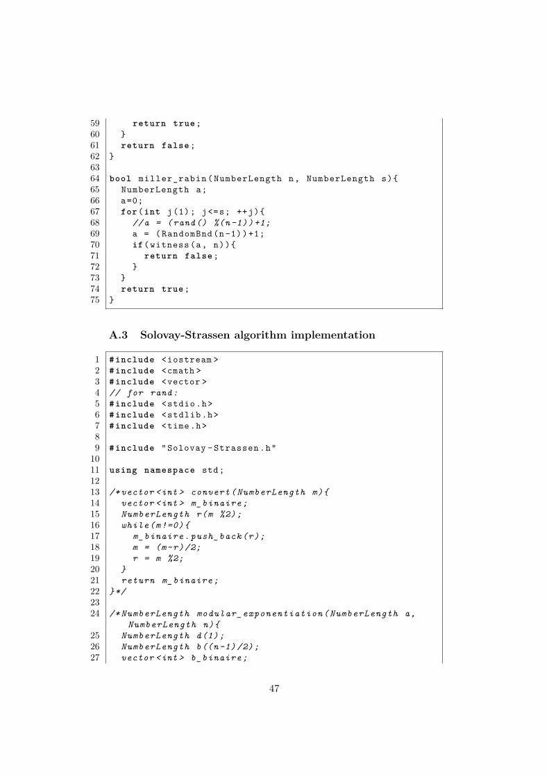
59 return true;60 }61 return false;62 }6364 bool miller_rabin ( NumberLength n, NumberLength s){65 NumberLength a;66 a=0;67 for(int j(1); j<=s; ++j){68 //a = (rand () %(n -1))+1;69 a = ( RandomBnd (n -1))+1;70 if( witness (a, n)){71 return false;72 }73 }74 return true;75 }

A.3 Solovay-Strassen algorithm implementation

1 # include <iostream >2 # include <cmath >3 # include <vector >4 // for rand:5 # include <stdio.h>6 # include <stdlib .h>7 # include <time.h>89 # include "Solovay - Strassen .h"

1011 using namespace std;1213 /* vector <int > convert ( NumberLength m){14 vector <int > m_binaire ;15 NumberLength r(m %2);16 while(m!=0){17 m_binaire . push_back (r);18 m = (m-r)/2;19 r = m %2;20 }21 return m_binaire ;22 }*/2324 /* NumberLength modular_exponentiation ( NumberLength a,

NumberLength n){25 NumberLength d(1);26 NumberLength b((n -1) /2);27 vector <int > b_binaire ;

47

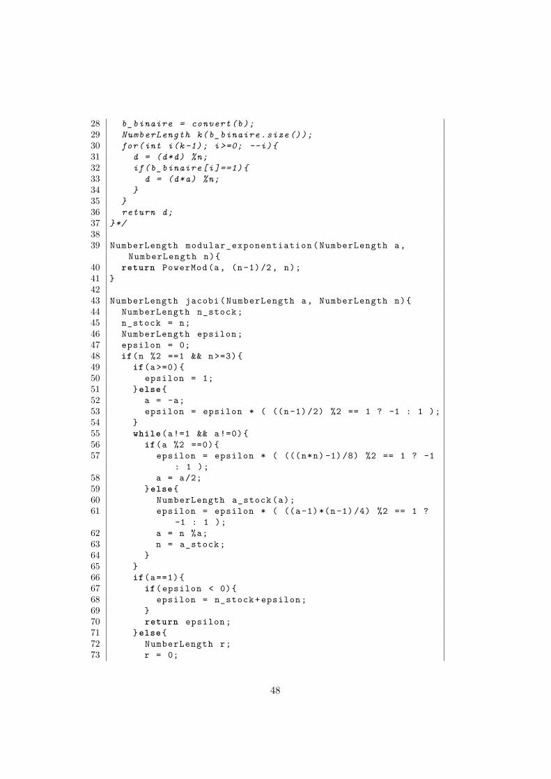
28 b_binaire = convert (b);29 NumberLength k( b_binaire .size ());30 for(int i(k -1); i >=0; --i){31 d = (d*d) %n;32 if( b_binaire [i ]==1){33 d = (d*a) %n;34 }35 }36 return d;37 }*/3839 NumberLength modular_exponentiation ( NumberLength a,

NumberLength n){40 return PowerMod (a, (n -1) /2, n);41 }4243 NumberLength jacobi ( NumberLength a, NumberLength n){44 NumberLength n_stock ;45 n_stock = n;46 NumberLength epsilon ;47 epsilon = 0;48 if(n %2 ==1 && n >=3){49 if(a >=0){50 epsilon = 1;51 }else{52 a = -a;53 epsilon = epsilon * ( ((n -1) /2) %2 == 1 ? -1 : 1 );54 }55 while (a!=1 && a!=0){56 if(a %2 ==0){57 epsilon = epsilon * ( (((n*n) -1) /8) %2 == 1 ? -1

: 1 );58 a = a/2;59 }else{60 NumberLength a_stock (a);61 epsilon = epsilon * ( ((a -1) *(n -1) /4) %2 == 1 ?

-1 : 1 );62 a = n %a;63 n = a_stock ;64 }65 }66 if(a==1){67 if( epsilon < 0){68 epsilon = n_stock + epsilon ;69 }70 return epsilon ;71 }else{72 NumberLength r;73 r = 0;

48

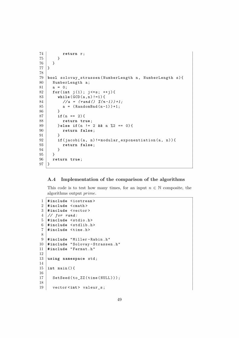
74 return r;75 }76 }77 }7879 bool solovay_strassen ( NumberLength n, NumberLength s){80 NumberLength a;81 a = 0;82 for(int j(1); j<=s; ++j){83 while (GCD(a,n)!=1){84 //a = (rand () %(n -1))+1;85 a = ( RandomBnd (n -1))+1;86 }87 if(n == 2){88 return true;89 }else if(n != 2 && n %2 == 0){90 return false;91 }92 if( jacobi (a, n)!= modular_exponentiation (a, n)){93 return false;94 }95 }96 return true;97 }

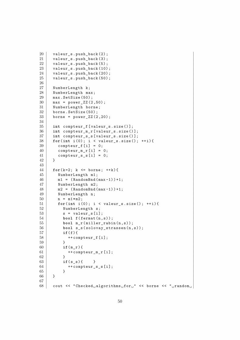
A.4 Implementation of the comparison of the algorithms

This code is to test how many times, for an input n ∈ N composite, thealgorithms output prime.

1 # include <iostream >2 # include <cmath >3 # include <vector >4 // for rand:5 # include <stdio.h>6 # include <stdlib .h>7 # include <time.h>89 # include "Miller -Rabin.h"

10 # include "Solovay - Strassen .h"11 # include " Fermat .h"1213 using namespace std;1415 int main (){1617 SetSeed ( to_ZZ (time(NULL)));1819 vector <int > valeur_s ;

49

20 valeur_s . push_back (2);21 valeur_s . push_back (3);22 valeur_s . push_back (5);23 valeur_s . push_back (10);24 valeur_s . push_back (20);25 valeur_s . push_back (50);2627 NumberLength k;28 NumberLength max;29 max. SetSize (50);30 max = power_ZZ (2 ,50);31 NumberLength borne;32 borne. SetSize (50);33 borne = power_ZZ (2 ,20);3435 int compteur_f [ valeur_s .size ()];36 int compteur_m_r [ valeur_s .size ()];37 int compteur_s_s [ valeur_s .size ()];38 for(int i(0); i < valeur_s .size (); ++i){39 compteur_f [i] = 0;40 compteur_m_r [i] = 0;41 compteur_s_s [i] = 0;42 }4344 for(k=2; k <= borne ; ++k){45 NumberLength m1;46 m1 = ( RandomBnd (max -1))+1;47 NumberLength m2;48 m2 = ( RandomBnd (max -1))+1;49 NumberLength n;50 n = m1*m2;51 for(int i(0); i < valeur_s .size (); ++i){52 NumberLength s;53 s = valeur_s [i];54 bool f( fermat (n,s));55 bool m_r( miller_rabin (n,s));56 bool s_s( solovay_strassen (n,s));57 if(f){58 ++ compteur_f [i];59 }60 if(m_r){61 ++ compteur_m_r [i];62 }63 if(s_s){ }64 ++ compteur_s_s [i];65 }66 }6768 cout << " Checked � algorithms �for�" << borne << "� random �

50

composite � numbers �<�" << max << "." << endl;69 for(int i(0); i < valeur_s .size (); ++i){70 cout << "For�s�=�" << valeur_s [i] << ",�the� Fermat �

algorithm � makes�" << compteur_f [i] << "� errors ."<< endl;

71 cout << "For�s�=�" << valeur_s [i] << ",�the�Miller -Rabin� algorithm �makes�" <<compteur_m_r [i] << "� errors ." << endl;

72 cout << "For�s�=�" << valeur_s [i] << ",�the�Solovay - Strassen � algorithm �makes�" <<compteur_s_s [i] << "� errors ." << endl;

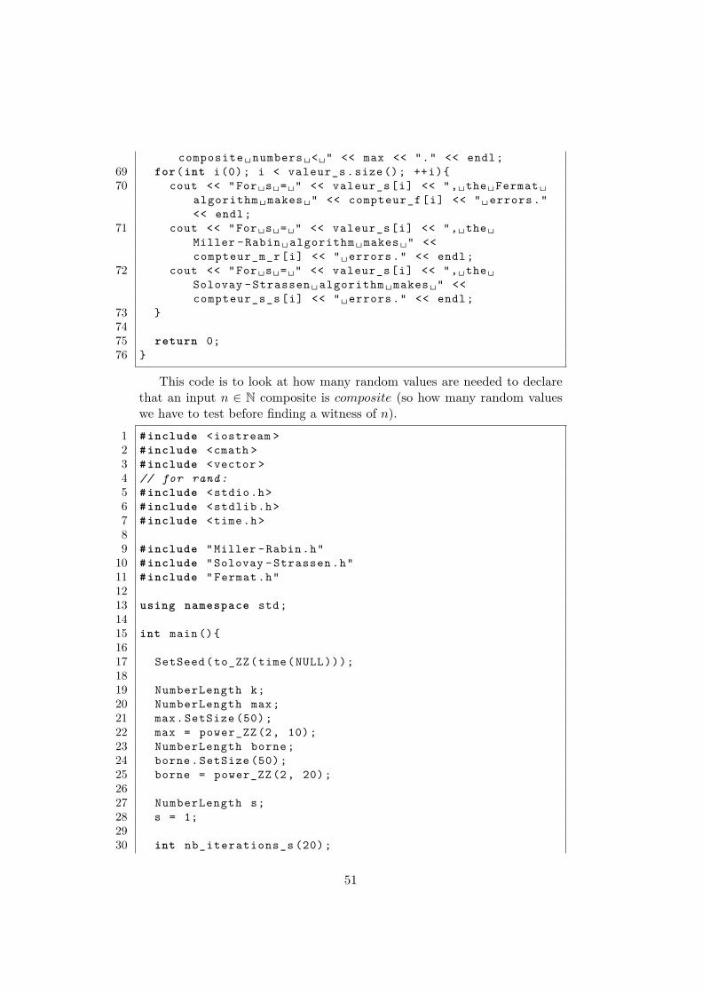
73 }7475 return 0;76 }

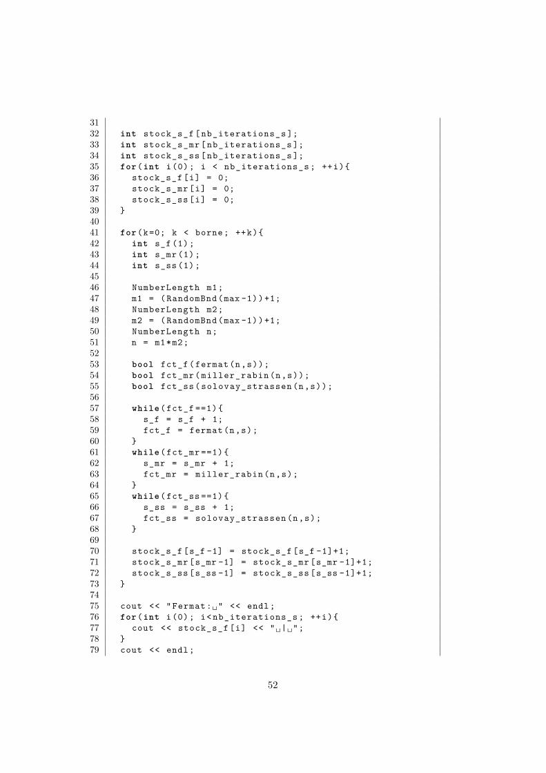
This code is to look at how many random values are needed to declarethat an input n ∈ N composite is composite (so how many random valueswe have to test before finding a witness of n).

1 # include <iostream >2 # include <cmath >3 # include <vector >4 // for rand:5 # include <stdio.h>6 # include <stdlib .h>7 # include <time.h>89 # include "Miller -Rabin.h"

10 # include "Solovay - Strassen .h"11 # include " Fermat .h"1213 using namespace std;1415 int main (){1617 SetSeed ( to_ZZ (time(NULL)));1819 NumberLength k;20 NumberLength max;21 max. SetSize (50);22 max = power_ZZ (2, 10);23 NumberLength borne;24 borne. SetSize (50);25 borne = power_ZZ (2, 20);2627 NumberLength s;28 s = 1;2930 int nb_iterations_s (20);

51

3132 int stock_s_f [ nb_iterations_s ];33 int stock_s_mr [ nb_iterations_s ];34 int stock_s_ss [ nb_iterations_s ];35 for(int i(0); i < nb_iterations_s ; ++i){36 stock_s_f [i] = 0;37 stock_s_mr [i] = 0;38 stock_s_ss [i] = 0;39 }4041 for(k=0; k < borne ; ++k){42 int s_f (1);43 int s_mr (1);44 int s_ss (1);4546 NumberLength m1;47 m1 = ( RandomBnd (max -1))+1;48 NumberLength m2;49 m2 = ( RandomBnd (max -1))+1;50 NumberLength n;51 n = m1*m2;5253 bool fct_f( fermat (n,s));54 bool fct_mr ( miller_rabin (n,s));55 bool fct_ss ( solovay_strassen (n,s));5657 while (fct_f ==1){58 s_f = s_f + 1;59 fct_f = fermat (n,s);60 }61 while ( fct_mr ==1){62 s_mr = s_mr + 1;63 fct_mr = miller_rabin (n,s);64 }65 while ( fct_ss ==1){66 s_ss = s_ss + 1;67 fct_ss = solovay_strassen (n,s);68 }6970 stock_s_f [s_f -1] = stock_s_f [s_f -1]+1;71 stock_s_mr [s_mr -1] = stock_s_mr [s_mr -1]+1;72 stock_s_ss [s_ss -1] = stock_s_ss [s_ss -1]+1;73 }7475 cout << " Fermat :�" << endl;76 for(int i(0); i< nb_iterations_s ; ++i){77 cout << stock_s_f [i] << "�|�";78 }79 cout << endl;

52

8081 cout << "Miller - Rabin:�" << endl;82 for(int i(0); i< nb_iterations_s ; ++i){83 cout << stock_s_mr [i] << "�|�";84 }85 cout << endl;8687 cout << "Solovay - Strassen :�" << endl;88 for(int i(0); i< nb_iterations_s ; ++i){89 cout << stock_s_ss [i] << "�|�";90 }91 cout << endl;9293 return 0;94 }

53

References

[1] Thomas Cormen, Charles Leiserson, Ronald Rivest, and Clifford Stein.Introduction à l’algorithmique, 2ème édition. Dunod, 2002.

[2] Michel Demazure. Cours d’algèbre. Primalité. Divisibilité. Codes.Cassini, 1997.

[3] Neal Koblitz. A Course in Number Theory and Cryptography. Springer-Verlag, 1988.

[4] Victor Shoup. A Computational Introduction to Number Theory andAlgebra. Cambridge University Press, 2005.

54

randomized and deterministic primality testing - algo

Documents