Elliptic Curves

Notes from a series of lectures by

Rene SchoofUniversita di Roma “Tor Vergata”

Guest Lecturers:Henri Darmon, Isabelle Dechene, Eyal Goren,Andrew Granville and Kiran Kedlaya

The 2008 Barbados Workshop on Computational ComplexityMarch 2nd – March 9th, 2008

Organizer:Denis Therien

Scribes:Anil Ada, Anne Broadbent, Arkadev Chattopadhyay, Matei David, Laszlo Egri, Mark Mercer,Nitin Saxena, Valentina Settimi, John Voight.

1

2

Lecture 1. Introduction

Lecturer: Rene Schoof Scribe: Anne Broadbent

“The kind of computer science we do, we like to call math.Rene will be showing us some real mathematics.”— Denis Therien

1.1 Introduction

The topic of these lectures are applications of elliptic curves. The main applications we will seeare:

1. factoring integers

2. primality testing

3. discrete logarithm

Scribe notes: Rene Schoof will give five morning lectures, each approximately2 hours each.Late afternoon lectures last approximately 1.5 hours and will be given by different speakers eachday.

1.2 Factoring, primality testing and “p − 1” algorithms

Factoring is the jungle— Rene Schoof

TheRabin-Miller algorithm is a very efficient “probable” primality test. Applied ton ∈ Z>0 ,it can give two answers:

1. n is not prime

2. n could be prime.

In case 1, the answer is guaranteed to be correct and so we knowthatn is not prime. Case 2,is not so favourable, and all we can do is repeat the test to increase our confidence level (if the testalways passes, we conclude thatn is “very likely” a prime). This of course, does not give a proofof primality.

Depending on the situation, we can ask the following questions:

1. If n is not prime, what are its factors?

3

2. If n “very likely” prime, can we have a proof of primality?

Note: There exists a deterministic polynomial time primality test by Agrawal, Kayal and Sax-ena.

Let p be prime, thenp− 1 = #(Z/pZ)∗ is theorder of Z mod p. We will also writeZ/pZ =Fp ; it is a finite cyclic group.

Proposition 1. LetA be a finite multiplicative Abelian group of ordern (#A =n). Then:

1. ∀a ∈ A, an = 1

2. ∀a ∈ A, ord(a) dividesn.

1.2.1 p − 1 factoring

Algorithm 1 is due to Pollard and goes back to the ’70ies.

Algorithm 1 p − 1 factoringinput: n ∈ Z>0 to be factoredoutput: non-trivial factor ofn or⊥

1. Choose a boundB which will determine the time spent running the algorithm

2. Pick a randomx ∈ (Z/pZ)∗ with gcd(x, n) = 1 (use Euclidean algorithm to test this)

3. LetM be the product of all prime powers smaller thanB:

M =∏

qe(q)<B

qe(q) , (1.1)

whereq is prime andqe(q) is the largest power ofq that is less thanB. By a version of theprime number theorem,M ∼ exp(B)

4. Computegcd(xM − 1, n) = m by first computingxM (mod n) using modular exponentia-tion

5. If m 6= 1, outputm, otherwise output⊥

The work required for the modular exponentiation is inO(B log2 n), while the rest of step 4 isin O(log3 n). The total work of algorithm 1 is inO(B) .

We now havegcd(XM−1, n), which obviously dividesn. Let’s see under which circumstancesthis algorithm gives us something useful.

If gcd(XM − 1, n) 6= 1, it is divisible by a primep|n

⇔ xM − 1 ≡ 0 (mod p) (1.2)

⇔ xM ≡ 1 (mod p) . (1.3)

4

By Proposition 1,xp−1 ≡ 1 (mod p) (Fermat’s little theorem).

xM ≡ 1 (mod p) (1.4)

⇔p − 1 dividesM (1.5)

⇔p − 1 is B-smooth (1.6)

Where the before-last equivalence is “not exactly an equivalence, but true in practice”. Note thatwe say thatp − 1 is B-smoothif all primes dividingp − 1 are less thanB.

Hence we have success in algorithm 1 ifn is divisible by a primep with the property thatp− 1is B-smooth. The problem is that in practice, if you want to factor n, you do not knowp, and youdo not know for whichB, the numberp− 1 is B-smooth! The worst case arises whenn = pq withp, q ≈ √

n, andp− 1 not smooth for anyB, i.e.p− 1 = 2r for r prime,r ≈ 12

√n. The total work

in this case is inO(B) ∈ O(√

r). The naive factoring algorithm runs in the same time, hence wehaven’t done much better.

We can formally analyze the probability that this algorithmwill work, and conclude that thealgorithm almost never works!

5

1.2.2 p − 1 primality test (Pocklington 1916)

We now describe an algorithm for primality testing, it is based on a proposition:

Proposition 2. Let n − 1 = QR. If for every primeq|Q there existsa ∈ (Z/nZ)∗ with aQ ≡ 1

(mod n) andgcd(aQq −1, n) = 1, then any prime divisorp ofn satisfiesp ≡ 1 (mod Q) (including

p > Q). In particular, if Q >√

n, we have thatn is prime.

Proof. Let q be a prime divisor ofQ, with qm the exact power ofq dividing Q.

Claim: b = aQ

qm ∈ (Z/pZ)∗ has orderqm. This is becausebqm ≡ aQ ≡ 1 (mod n), so the

order ofb dividesqm. Now, bqm−1= a

Qq in (Z/nZ)∗. We also know thatbqm ≡ 1 in (Z/pZ)∗, so

bam−1= a

Qq in (Z/pZ)∗.

Couldbqm−1= 1? If so, we havea

Qq ≡ 1 (mod p). Sincep|(a

Qq − 1), p| gcd(a

Qq − 1, n) is not

true. So the claim is true also in(Z/pZ)∗.Hence:

qm|#(Z/pZ)∗ = p − 1 (1.7)

p ≡ 1 (mod qm)∀q (1.8)

p ≡ 1 (mod Q)

Scribe notes: in what follows, the speaker’s original presentation has been modified to highlightthe algorithm and its properties.

Algorithm 2 p − 1 primality testinput: n ∈ Z>0 (supposen passes the Miller-Rabin test)output: “n is prime” or⊥

1. Using computational resources available, find all small prime factors ofn − 1. Let Q be theproduct of these primes. Letn − 1 = QR (we callR thecofactor).

2. Now, three things can happen

(a) (almost never)Q >√

n. For each primeq|Q (suppose we already have a proof of pri-mality for q, if need be, call algorithm 2 recursively!), we need to find a correspondinga as in proposition 2. Picka at random inZ/nZ. Check thataQ ≡ 1 (mod n), and

thatgcd(aQq − 1, n) = 1 . If all tests succeed, output “n is prime”.

(b) (usually)R not prime but cannot factor within reasonable time. Give up and output⊥.

(c) (occasionally)n − 1 = QR, with Q <√

n andR >√

n passes the Miller-Rabin test.Reverse the roles ofQ andR, at which point we fall back into case (a).

The goal of algorithm 2 is to check that the conditions of proposition 2 are satisfied, withQ >

√n. It is clear that this is what is accomplished and that the output of the algorithm is correct.

6

What about the choice ofa in step (a)? Ifn is prime, then(Z/nZ)∗ is cyclic, suppose it isgenerated byg. Takea = gR. ThenaQ = gRQ = gn−1 ≡ 1 (mod n) (Fermat’s little theorem),

andgcd(aQq − 1, n) = 1 because if not,a

Qq ≡ g

n−1g ≡ 1 (mod n), which cannot happen. So ifn

is prime, our method of pickinga at random should give good results.How about the complexity of the algorithm? ComputingaQ (mod n) (modular exponentia-

tion) requires work inO(log3 n). Thegcd computation is also polynomial.But will it work? In practice, because of (a), (b) and (c), we won’t make much progress. For

instance, takingn ∼ 101000 gives a probability of success that is low.

1.3 Elliptic Curves

Elliptic curves are an “old” subject— much older than computers. Our study is motivated byalgorithmic applications. In the previous section, we saw two p − 1 algorithms:

• factoring: Success if there existsp|n such thatp − 1 is B-smooth.

• primality: Success ifp− 1 = QR where the factored partQ is >√

n or p− 1 = QR wherethe factored partQ <

√n andR is a probable prime.

These algorithms have in common the fact that they use group-theoretic statements, but they needto be lucky to actually work.

Now, our key idea will be to replace(Z/pZ)∗ by groups of points on elliptic curves. Theadvantage here is that there are many elliptic curves to we can try, thus eliminating the need for“luck”.

An elliptic curveover a fieldk (R, C, Fq) is given by the cubic curve:

Y 2 + a1XY + a3Y = X3 + a2X2 + a4X + a6 , (1.9)

wherea1, a2, a3, a4, a6 ∈ k (no, it’s not a mistake thata5 is missing). Define the following:

b2 = a21 + 4a2

b4 = a1a3 + 2a4

b6 = a23 + 4a6

b8 = a21a6 + 4a2a6 − a1a3a4 + a2a

23 − a2

4

c4 = b22 − 24b4

c6 = −b32 + 36b2b4 − 216b6

∆ = −b22b8 − 8b3

4 − 27b26 + 9b2b4b6 .

We’re interested in nonsingular curves with discriminant∆ 6= 0. We also have the relationship

1728∆ = c34 − c2

6 . (1.10)

7

If the characteristic of the field isn’t 2, we can divide by 2 and complete the square:

(Y +a1X + a3

2)2 = X3 + (a2 +

a21

4)X2 + a4X + (

a23

4+ a6) , (1.11)

which can be written as:Y 2

1 = X3 + a′2X

2 + a′4X + a′

6 , (1.12)

with Y1 = Y + a1X/2 + a3/2. If the characteristic is also not 3, then we can letX ← X+a′

2

3to get

the curveY 2 = X3 + AX + B . (1.13)

The discriminant becomes∆ = −16(4A3 +27B2), and the condition that the curve be nonsingularis of course still verified by∆ 6= 0 .

Some notation: elliptic curves are denotedE, andE(k) denotes the set of points onE withcoordinates ink, together with a special “symbolic” point(∞,∞) called the point at infinity.

Now, we want to show our main point of this lecture, that is, that we can giveE(k) the structureof a group in a natural way. Our approach is a practical one; more mathematical approaches wouldbe possible.

Figure 1.1: Elliptic curve addition (source: certicom.com)

1.3.1 Group Law on Elliptic Curves

Consider the right-hand side ofY 2 = X3 +AX +B, which is a cubic. A cubic can have either oneor two roots. When we take the square root of this cubic, we get two different families of ellipticcurves, as illustrated in figures 1.1 and 1.2 (our illustrations are done with underlying fieldk = R) .

8

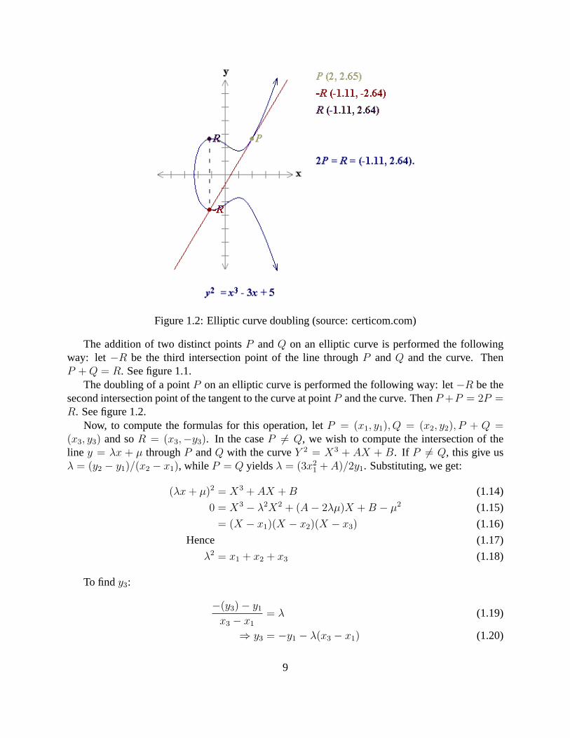
Figure 1.2: Elliptic curve doubling (source: certicom.com)

The addition of two distinct pointsP andQ on an elliptic curve is performed the followingway: let −R be the third intersection point of the line throughP andQ and the curve. ThenP + Q = R. See figure 1.1.

The doubling of a pointP on an elliptic curve is performed the following way: let−R be thesecond intersection point of the tangent to the curve at point P and the curve. ThenP +P = 2P =R. See figure 1.2.

Now, to compute the formulas for this operation, letP = (x1, y1), Q = (x2, y2), P + Q =(x3, y3) and soR = (x3,−y3). In the caseP 6= Q, we wish to compute the intersection of theline y = λx + µ throughP andQ with the curveY 2 = X3 + AX + B. If P 6= Q, this give usλ = (y2 − y1)/(x2 − x1), while P = Q yieldsλ = (3x2

1 + A)/2y1. Substituting, we get:

(λx + µ)2 = X3 + AX + B (1.14)

0 = X3 − λ2X2 + (A − 2λµ)X + B − µ2 (1.15)

= (X − x1)(X − x2)(X − x3) (1.16)

Hence (1.17)

λ2 = x1 + x2 + x3 (1.18)

To findy3:

−(y3) − y1

x3 − x1

= λ (1.19)

⇒ y3 = −y1 − λ(x3 − x1) (1.20)

9

Explicitly,

x3 = −x1 − x2 + λ2 (1.21)

y3 = −y1 − λ(x3 − x1) . (1.22)

Where eitherλ = (y2 − y1)/(x2 − x1) (if P 6= Q) or λ = (3x21 + A)/(2y1) (if P = Q).

We also add the rule that for any pointP = (x, y), −P = (x,−y) and theP +−P = (∞,∞).We now have all the tools to compute on an elliptic curve, and we can indeed show that this

operation forms a commutative group (associativity is harder to prove).We now give two examples overZ/5Z:

We cannot draw a picture anymore. A picture would be quite pointless. . . literally.— Rene Schoof

Example 1 (Adding points overZ/5Z). Let E : Y 2 = X3 + X + 1 overZ/5Z. First, we checkthat this is an elliptic curve:

∆ = −16(4 · 13 + 27 · 12) ≡ −1(−1 + 2) 6≡ 0 (mod 5) . (1.23)

LetP = (0, 1). We want to computeP + P . Using the given formulas, we get:

λ =3 · 02 + 1

2 · 1 ≡ 3 (mod 5) (1.24)

x3 = −0 − 0 + 32 = 9 ≡ −1 (mod 5) (1.25)

y3 = −1 − 3(−1 − 0) ≡ 2 (mod 5) . (1.26)

SoP + P = (−1, 2) and we can check that it sits on the curve.

10

Example 2 (Determining all points overZ/5Z). Consider the curveE given in the previous ex-ample. We want to list all points onE.

First, we compute the squares inZ/5Z . We get12 = 1, 22 = −1, (−2)2 = −1, (−1)2 = 1, so1 and−1 are squares, with roots1,−1 and2,−2, respectively. We proceed as in table 1.1 toget the 8 points of the curve, to which we add the point at infinity.

X X3 X3 + X + 1 points0 0 1 (0, 1), (0,−1)1 1 -2 none2 -2 1 (2, 1), (2,−1)-2 2 1 (−2, 1), (−2,−1)-1 -1 -1 (−1, 2), (−1,−2)

Table 1.1: Finding points on the curveY 2 = X3 + X + 1 overZ/5Z

A further question we can ask is whether the group is isomorphicto Z/9Z or Z/3Z × Z/3Z.The answer isZ/9Z since we eliminate the possibility ofZ/3Z × Z/3Z by takingP = (0, 1), andfinding thatp + p 6= −p. (See example 1.)

11

Lecture 2. Prime and Smooth Numbers in Intervals

Lecturer: Andrew Granville Scribe: Arkadev Chattopadhyay

Here we go through a quick survey of results from analytic number theory on the asymptoticbehavior of the number of primes and smooth numbers in a giveninterval.

2.1 Prime numbers

Gauss made the conjecture that the number of primes uptox, denoted byπ(x), is roughlyx/ log x.Gauss’s guessed estimate ofπ(x), called the logarithmic integral estimate and denoted by Li(x),is inspired by the fact that he expected (aided by his very impressive mental calculation of the first“few” primes) the density of primes to be about1/ log n aroundn. More precisely,

Li(x) =

∫ x

2

dt

log t.

Integrating above by parts, we get

Li(x) =x

log x

(1 +

∞∑

k=1

k!

(log x)k

).

The first big progress towards understanding the relationship of π(x) and Li(x) was made in1896 by Hadamard and de la Vallee Poussin who proved the following:

Theorem 1(Prime Number Theorem). limx→∞π(x)

x/ log x→ 1.

Although the Prime Number Theorem tells us that the density of primes asymptotically agreewith Gauss’s estimate, it does not tell us much about the error functionπ(x) − Li(x).

Using Fourier Analysis, we believe that10316 is the right point where Gauss’s estimate isinadequate. Moreover, it seems from the data that

∣∣∣∣π(x) −∫ x

2

dt

log t

∣∣∣∣ < 2x1/2(log x)A (2.27)

It is remarkable that the correctness of the above statementis equivalent to the famous RiemannHypothesis.

Riemann defined a zeta function, denoted byζ, by the following series for Re(s) > 1:

ζ(s) =∑

n≥1

1

ns.

Although ζ(s) has a pole ats = 1, it can be analytically continued to the set of every othercomplex number i.e.C − 1. This analytic continuation is called the Riemann zeta function.

12

Conjecture 1 (Riemann’s Hypothesis). If ζ(s) = 0, then Re(s) ≤ 1/2.

Riemann knew that every negative even integer is a zero of the zeta function but called themthe trivial zeroes. His hypothesis could be reformulated assaying “Every non-trivial zero of thezeta function occurs on the Re(s) = 1/2 line”. The proof of the Prime Number Theorem followedby establishing the following key fact:

Fact 1 (Hadamard and de la Vallee Poussin). The Prime Number Theorem is equivalent to sayingthat ζ(s) 6= 0 if Re(s) ≥ 1.

It was totally surprising when in 1949 Erdos/Selberg provided an elementary proof the PrimeNumber Theorem.

Riemann had showed also the following remarkable fact:

π(x) −∫ x

2

dt

log t≈ −

∑

ρ;ζ(ρ)=0

xρ

ρ log x(2.28)

In (2.28)ρ in the summation on the RHS has positive real part. Assumeρ = β + iα. Note that

∣∣∣∣xρ

ρ log x

∣∣∣∣ =xβ

|ρ| log x.

Hence, taking absolute values on both sides of (2.28) we get

|Error| ≤∑

ρ=β+iα

xβ

|ρ| log x.

Thus,

|Error| ≤ xmaxβ

log x

∑ 1

|ρ|(log x)A.

Thus, assuming the Riemann Hypothesis we see that maxβ = 1/2 and plugging this into theabove gives us the refined estimate onπ(x) provided by (2.27).

2.1.1 Consequences for primality testing

Our guess estimate for the number of primes in the interval[x, x + y] i.e. π(x + y) − π(x)will be roughly y/ log x where2 < y < x1−ǫ. However, our estimate does not give us even aninteger for too small values ofy. May be it is true forx > y > (log x)3. It can be proved tobe true forx > y > x2/3. On the other hand, the Riemann Hypothesis implies that it holds forx > y > x1/2 log x.

Aside Remark 1. In 1932 Cramer conjectured that there is always a prime in(x, x + (log x)2).This conjecture is still open.

13

This discussion brings us to the question on how large could the gap between consecutiveprimes be? Letp1 = 2 < p2 = 3 < p3 < p4 < · · · be the sequence of consecutive prime numberswith pi denoting theith prime. The prime number theorem tells us that on the averagepn+1 − pn isaboutlog pn. Erdos and others proved that the gap between consecutive primescan be arbitrarilylarge compared to the average. More precisely, it was shown

maxpn≤x pn+1 − pn > 2e−γ log x(log log x) log log log log x

(log log log x)2(2.29)

In particular, (2.29) implies that

limn→∞

suppn+1 − pn

log pn

→ ∞.

By contrast, one can ask the question how small can the gap between consecutive primes be?In a recent breakthrough, Goldston, Pintz and Yildirim showed that the gap can be arbitrarily smallcompared to the average i.e.

limn→∞

infpn+1 − pn

log pn

→ 0.

The result above constitutes important progress to the twinprime conjecture that says there areinfinitely many pairs of primes that are separated by 2 i.e.limn→∞ inf pn+1 − pn = 2.

We come back to the application to the Goldwasser-Kilian (GK) algorithm for primality testingusing elliptic curves. Recall that such a curveE is given by equations of the formy2 = x3 + ax +b modp for some primep. In the morning lecture, we saw that the points on such a curveform anabelian group of orderNp(E) with p − 2

√p < Np(E) < p + 2

√p. The idea of the GK algorithm

is to modify Pocklington’s algorithm by working with the group of points on a randomly generatedcurveE instead of the fixed groupZ/nZ. What this modified algorithm requires (in practice) isthat the number of points on the curveE be either a prime or twice a prime. In other words, weare interested in the existence of a primeq such that

x =p − 2

√p + 1

2< q <

p + 2√

p + 1

2≈ x + 2

√x.

What we can prove is that100% of intervals(x, x + x1/1000) i.e. “almost allx” have aboutx1/1000

log xmany primes. Consequently, Goldwasser-Kilian will prove the primality of a prime number

almost all of the time. Adleman-Huang bettered GK by workingwith random hyperelliptic curvesoverZp. The number of points on such a curve lies in the interval(p2 − cp3/2, p2 + cp3/2). Thus,we need to find primes in the interval(x, x + x3/4) and with even higher probability than GK,Adleman-Huang (AH) succeeds. Both AH and GK tests are mostly of historical importance nowas AKS provides a determinisitc poly time test for primality.

14

2.2 Smooth Numbers

A numbern is calledy-smooth if every prime that dividesn is no larger thany. We denote byΨ(x, y) the number of integers less than or equal tox that arey-smooth. ObviouslyΨ(x, x) = x.

Let us estimateΨ(x, x) − Ψ(x, y). Assumex > y >√

x. Then,

Ψ(x, x) − Ψ(x, y) =#n = pm ≤ x : p > y=

∑

y<p≤x

#m ≤ x

p

≈∑

y<p≤x

x

p

Thus,

Ψ(x, y) ≈ x

(1 −

∑

y<p≤x

1

p

).

It can be shown that ∑

p≤x

1

p= log log x + C + O

( 1

log x

).

So,∑

y<p≤x

1

p≈ log

(log x

log y

).

If x = yu and1 ≤ u ≤ 2, then

Ψ(x, x1/u

)≈ x(1 − log u).

If 2 < u < 3, then following what we did before gets us

Ψ(x, x1/u

)≈ x

(1 −

∑

y<p≤x

1

p+

∑

p,q>y;pq≤x

1

pq

).

2.2.1 Largeru

We will try to estimateΨ(x, y) recursively having established it for small values ofu. Noting that

Ψ(x, x) − Ψ(x, y) =∑

y<p≤x

#pm ≤ x : m is p-smooth.

This immediately gives the recursive relation

Ψ(x, x) − Ψ(x, y) =∑

y<p≤x

Ψ(x

p, p

).

15

AssumingΨ(x, x1/u) ∼ xρ(u), we get

x(1 − ρ(u)

)=

∑

y<p≤x

x

pρ

(log(x/p)

log p

)(2.30)

Applying the Prime Number Theorem,

RHS of (2.30)≈∫ x

y

x

t log tρ

(log(x/t)

log t

)dt (2.31)

The RHS of (2.31) has an error term that has to be eventually taken care of. Substitutet = yw sothat log t = w log y. It is easily verified then

dt

t log t=

dw

w.

Plugging this substitution into the RHS of (2.31) we get

RHS of (2.31)≈ x

∫ u

w=1

ρ

(u

w− 1

)dw

w(2.32)

Substitutev = u/w, wherebydv/v = −dw/w and so we get

1 − ρ(u) =

∫ u

v=1

ρ(v − 1)dv

v(2.33)

To summarize, what we have proved is thatΨ(x, x1/u)/x → ρ(u) whereρ(u) is a complicatedfunction that is given by the integral equation (2.33). The key thing to remember is thatΨ(x, y) =xρ(u) where,

ρ(u) ≈ 1

uu(2.34)

andx = yu. This remains provably true for

y > e(log log x)5/3+ǫ

(2.35)

Surprisingly, the Riemann Hypothesis is equivalent to the above estimate holding fory >(log x)2+ǫ.

16

2.2.2 Lenstra’s algorithm

Lenstra’s algorithm modifies Pollard’sp − 1 algorithm of factoring by working with the group ofpoints on an elliptic curve. Roughly, we estimate the time that we want the algorithm to work. Sayit is B. Then letM =

∏qǫ<B qǫ be aB-smooth number. We choose a random elliptic curveE

(overZ/nZ) and a pointP on it. Then we computeP + · · ·+M times· · ·+P using the group lawfor adding points onE. Letp be a prime factor ofn. If the curveEp (the oneE induces overZ/pZvia reduction modp) has an order that isB-smooth and the order of all otherEq, whereq|n, are notB-smooth then this addition process identifiesp as a factor ofn. Since the order of the group ofpoints onEp lies betweenp−2

√p+1 andp+2

√p+1, we are interested to findB-smooth numbers

in this interval1. The relationship betweenB andp is roughly given byB = O(log p)c for someconstantc if we want Lenstra’s algorithm to run in polytime w.r.t its input length (which islog n).Moreover the running bound of Lenstra’s algorithm works if the number ofB-smooth numbers inthis interval is what we would expect it to be according to estimate (2.34) i.e.4

√p/ρ(u)u where

y = x1/u = (log p)c = exp(c log log p). This is unfortunately smaller than the range for whichestimates provably work as given by (2.35).

1Note that corresponding to every number in this interval, wecan find an elliptic curve that has exactly that manypoints on it.

17

Lecture 3. Hasse’s Theorem

Lecturer: Rene Schoof Scribe: Laszlo Egri

Part 1

Before Rene’s lecture, Pavel shortly explained some probabilistic complexity classes. Primes is incoRP due to Rabin and Miller. Adleman and Huang showed that Primes is in RP and thereforePrimes is in coRP∩ RP= ZPP . Finally, in 2002 it was shown by AKS that Primes is in P. Notethat the generalized Riemann hypothesis implies that primesis in P.

A problemX ∈ ZPP if there exists a randomized polynomial time algorithmA such that

A(x) = 0 → x 6∈ X, x ∈ X → P (A(x) = 1) ≥ 1

3

A(x) = 1 → x ∈ X, x 6∈ X → P (A(x) = 0) ≥ 1

3.

More General Form

Here Rene shortly remarked that in general, an elliptic curve has theform y2 + a1xy + a3y =x3 + a2x

2 + a4x + a6 but usuallya1 = a2 = a3 = 0 and then we get the form which we use mostof the time.

Addition can be defined in the same way. Consider(x1, y1) + (x2, y2) = (x3, y3). The slope is

λ =

y2−y1

x2−x1if the two points are different

3x2+2a2x+a4x−a1y24+a1x+a3

if the two points are the same

x1 + x2 + x3 = λ2 + a1λ

−y3 + a1x3 + a3 = λ(x3 − x1) + y1

−(x, y) = (x,−y + a1x + a3).

Projective Coordinates

Let K be a field andE : y2 = x3 + Ax + B be an elliptic curve such thatchar(K) 6= 2, 3,A,B ∈ K and4A3 + 27B2 6= 0.

A projective planeP2 is defined as

P2 = (x, y, z) : (x : y : z) 6= (0, 0, 0) and(x : y : z) ≡ (x′ : y′ : z′)

if there existsc ∈ K∗ such thatcx = x′, cy = y′, cz = z′

18

We can define a map fromA2 (affine space) intoP2 as(x, y) 7→ (x : y : 1). We can also goback:

(x

z,y

z

)← (x : y : z) ∈ P2, z 6= 0

curve projective curve

We can see that the infinity point is

(∞,∞) =

z = 0

x = 0

y 6= 0 y = 1.

Work on a Computer

Let K = Z/pZ. Then we can determine

x3 = −x1 − x2 +

(y2 − y1

x2 − x1

)2

: y3 : 1

(here the calculation of the inverse of the denominator is expensive, it can be done using theEuclidean algorithm) or equivalently,

(−x1 − x2)(x2 − x1)2 + (y2 − y1)

2 : y2(y2 − x1)2 : (x2 − x1)

2

in O(log3p) time.

Exercises

Let E be an elliptic curvey2 = x3 + Ax + B over a fieldK = K such thatchar(K) 6= 2, 3. Let’sdetermine the number of points of order2 and3.

Points of order 2

Let P = (x, y). ThenP + P = 0 ↔ P = −P ↔ (x, y) = (x,−y) → y = 0 → x3 + Ax + B =0 → there are three points of order2.

Let n ∈ N. Assume thatK is an algebraically closed field. Define the set ofn-torsion pointsE[n] ⊂ E(K) to be the set of elements inE(K) which have ordern, i.e.

E[n] = P ∈ E(K) : P + · · · + P︸ ︷︷ ︸n

= (∞,∞).

ThenE[2] ∼= Z/2Z × Z/2Z.

19

Points of order 3

Let P = (x, y). Assume thatP + P + P = 0. ThenP + P = −P and−P = (x,−y). SoP +P = (x3, y3). Thenx3 = −x−x+λ2, whereλ = 3x2+A

2y. So(−2x+(3x2+A

2y)2, y3) = (x,−y).

It follows that(3x2 + A)2 = 3x(Ay2) = 12x(x3 + Ax + B) and3x4 + 6Ax2 + 12Bx − A2 = 0.So there are four zeroes. In fact,E[3] ∼= Z/3Z × Z/3Z.

Main Result

Let p be a prime andE be an elliptic curve overZ/pZ. The main result of today is:

1. E(Z/pZ) is almost cyclic, i.e. it can be generated by at most2 elements2;

2. p + 1 − 2√

p < #E(Z/pZ) < p + 1 + 2√

p.

Let K be the fieldFq whereq = pm (p is characteristic). HereE(K) = (x, y) : x, y ∈K, y2 = x3 +Ay +B∪∞,∞. LetK denote the algebraic closure ofK. ThenE(K) ⊂ E(K)(E(K) is an infinite group).

k(E) denotes a function field,k(E) = f1(x)+Y f2(x)g(x)

: f1, f2, g ∈ K[x], g(x) 6= 0.

Morphisms

Assume thatE1 andE2 are two elliptic curves over a fieldK. Then a morphismh from E1 toE2 maps any(x, y) ∈ E1(K) to (ϕ(x, y), ψ(x, y)) ∈ E1(K), whereϕ andψ are quotients ofpolynomials with coefficients inK. Morphismh must induce a group homomorphism and mustmap(∞,∞) to (∞,∞).

Examples

Let E : y2 = x3 + Ax + B. The following maps fromE to E are morphisms.

(x, y) 7→ (x,−y)

(x, y) 7→ (x, y)

(x, y) 7→ (∞,∞)

The zero morphism.Another example is the following. Let’s define(f +g)(x, y) := f(x, y)+g(x, y). Assume that

f = g = id. Then(f +g)(P ) = f(P )+g(P ) = P +P so(x, y)+(x, y) = (−2x+(3x2+A2y

)2 : y3)

and the function that maps(x, y) to (−2x + (3x2+A2y

)2 : y3) is a morphism.

2By almost cyclic we mean the following. Letℓ be a prime. Then ifℓ 6 |p − 1 then theℓ-part (Sylow subgroup) ofE(Z/pZ) is cyclic. If ℓ|p − 1 then the proportion ofE over(Z/pZ) with ℓ-part not cyclic≤ 1

ℓ3.

20

The Frobenius morphism. LetK be a field of characteristicp andα, β ∈ K. Clearly,(α+β)p =αp + βp. Let E be the elliptic curvey2 = x3 + Ax + B. Let P = (x, y).

(y2)p = (x3 + Ax + B)p

(yp)2 = (xp)3 + Apxp + Bp

Then the point(xp, yp) is on E : y2 = x3 + Apx + Bp. (∆(E) = ∆(E)p, where∆ is thediscriminant.)

Let ϕp : E → E be defined as(x, y) 7→ (xp, yp). Thenϕp is called thep-Frobenius morphism.Now letK = Fq. Then ifx ∈ K thenxq = x. (In particular, ifx ∈ Z/pZ thenxp ≡ x mod p.)

Consider

Eϕp→ E

ϕp→ ˜Eϕp→ . . .

ϕp→

˜

...E︸ ︷︷ ︸

m−times

.

Theq-Frobenius morphism is defined asϕq = ϕpm. Observe that the curvey2 = x3+Aqx+Bq

is the same asy2 = x3 + Ax + B, so in factϕq is fromE to E.Now letK = Fq ⊂ K = Fq. ThenK = α ∈ K : αq = α, i.e. Fq is the set of fixed points of

the mapα 7→ αq (from K to K). SoE(K) ⊂ E(K) whereE(K) = (x, y) : ϕq(x, y) = (x, y).

Part 2

Recall that Rene went over this section in finer detail in the first part of his next lecture.Recall the following. LetK = Fq (or Z/pZ). Consider the elliptic curveE : y2 = x3 +Ay+B

whereA,B ∈ K. ThenE(K) ⊆ E(K). (E(K) is a finite field.) A morphism fromE to itself iscalled an endomorphism. For example, theq-Frobeniusϕq(x, y) = (xq, yq) from E(K) to E(K)is an endomorphism.

Let E(K) = P ∈ E(K) : φq(P ) = P. Now ϕq(P ) = P ↔ (ϕ − id)(P ) = 0 ↔ P ∈ker(ϕq − id). It follows that

E(k) = ker(E(K)ϕq−id−→ E(K)).

Question: ifE1f→ E2 wheref is a morphism, then what isker(f)?

f : E → E : a morphism overK = End(E) is a ring. We can add, subtract, multiply:

(f + g)(P ) = f(P ) + g(P )

(f · g)(P ) = f(g(P ))

The identity for multiplication is the identity mapid. The identity for addition is the0-morphism(sends everything to∞). Let’s define[n] = id + · · · + id︸ ︷︷ ︸

n−times

, wheren ∈ N. Observe that the map

21

n 7→ [n] from Z to End(E) is an injective map. Also note that[n] : E(K) → E(K) defined asP 7→ P + · · · + P︸ ︷︷ ︸

n

is never the zero map.

An isogenybetween two elliptic curvesE1 andE2 is a morphismϕ : E1 → E2 such thatϕ(0) = 0. Two elliptic curves areisogenousif there is an isogenyϕ between them withϕ(E1) 6=0.

Let E1(K) andE2(K) be elliptic curves andf : E1 → E2 be a non-constant ”rational map”defined overK. Then composition withf induces an injection of function fields fixingK,

f ∗ : K(E1) ← K(E2)

f ∗g = f g.

We definedeg(f) = deg(formulas), anddeg(f) = degsep(f) · deginsep(f) or deg(f) =[K(E1) : f ∗K(E2)] (e.g.deg(id) = 1 anddeg(q − Frobenius) = q).

For example, lety2 = x3 + Ax + B andE[2]→ E.

(x, y) →(−2x +

(3x2 + A)2

4(x3 + Ax + B), yK(x)

)

K(E) ← K(E) = a(x + Y b(x) a(x) andb(x) are rational functions inx

← above is a degree4 extension.

−2x +(3x2 + A)2

4(x2 + Ax + B)← x

yK(x) ← y

Sodeg([2])=4.Fact:deg(fg) = deg(f)deg(g).Let f be a morphism fromE to E. If f is ap-th power where the characteristic of the field isp

thenf is inseparable. It is a fact that iff is separable then#ker(f) = deg(f).

Let Ef→ E. ThenI = f : E → E : inseparable ⊂ End(E). Note thatI is a two-sided

ideal andI is a strict subset ofEnd(E). For example,φq ∈ I.Let f = [p] wherep is the characteristic of the field. Then[p] ∈ I. The formula to express

f = (x, y) + · · · + (x, y) (p terms) is ap-th power.

Corollary 1.

p 6 |n ⇒ [n] 6∈ I

⇒ [n] is separable

#ker([n]) = deg(n)

22

Notice thatφq−id 6∈ I and it follows that#ker(φq−id) = deg(φq−id). (And#ker(φq−id) =#E(K).)

Let f : E → E. It is a fact thatdeg(f) = degnonsep(f)degsep(f) and therefore it is always thecase that#ker(f) = degsep(f)|deg(f). ⇒ deg(f) “kills” ker(f).

Let f : E → E be an isogeny. It is a fact that there exists a unique mapf v called the dualisogeny with the propertyf vf = [deg(f)]. These maps are inEnd(E). Here are some propertiesof f v:

f vv = f

(fg)v = f vgv

deg(f v) = deg(f)

(f + g)v = (f v + gv) (hardest to show)

Let’s do an example. LetFq = F2 = Z/2Z andE : y2 + xy = x3 + 1. Let’s compute the dualof φ2(x, y) = (x2, y2), deg(φ2) = 2.

[2] : E → E:

(x, y) + (x, y) =

(x2 +

1

x2, (y2 + 1)(1 +

1

x4) +

1

x2

)

=(V (x)2,W (x, y)2

)

Therefore

(V (x),W (x, y)) =

(x +

1

x, (y + 1)(1 +

1

x2) +

1

x

).

(x, y)g7→ (V (x),W (x, y)).

Observe thatφ2 g = [2] so the dual ofφ2 is g.Observe that multiplication is self-dual:

[n]v = [id + . . . + id]v = id + . . . id = [n].

Then[deg([n])] = [n]v[n] = [n]2 = [n2] and it follows thatdeg([n]) = n2. It follows that for everyn if p 6 |n then#ker([n]) = #E(K)[n] = n2. Then

⇒ E(K)[n] = P ∈ E(K) : P + . . . + P︸ ︷︷ ︸n

= ∞ ∼= Z/n × Z/n

⇒ E(K) ⊂ E(K)

⇒ E(K) can be generated by at most2 points.

Recall that

#E(K) = #ker(φq − id)

= deg(φq − id).

23

We define the tracet of a functionf ∈ End(E) as follows.t = trace = f + f v. Then

f + f v = (f + [1])(f v + [1]) − ff v − [1]

= [deg(f + 1)] − [deg(f)] − [1]

Therefore[f + f v] is in [Z] ⊂ End(E). For anyf we can write that

f 2 − (f + f v)f + f vf = 0 (in End(E))

f 2 − [t]f − [deg(f)] = 0

t anddeg(f) are integers so the maps∈ End(E).

Proposition 3 (Analogue of Riemann Hypothesis, 1933, Hasse). t2 ≤ 4deg(f).

Let m,n ∈ Z.

0 ≤ [deg([m] + [n]f)] = ([m] + [n]f)([m]v + [n]vf v)

= ([m] + [n]f)([m] + [n]f v)

= ([m]2 + [m][n](f + f v) + [n]2ff v)

= [n]2(

([m]

[n]

)2

+[m]

[n]t + deg(f))

It follows thatx2 − tx + deg(f) ∈ Z[x] has only≥ 0 values. Thereforet2 ≤ 4deg(f).

Corollary 2. #E(K) = q + 1 − t with |t| ≤ 2√

q.

Proof. We have

#E(K) = deg(φq − id)

= (φq − id)(φvq − id)

= q + 1 − t

andt2 ≤ 4deg(φq) = 4q as required.

24

Lecture 4. Constructing Elliptic Curves of Prescribed Order

Lecturer: Eyal Goren Scribe: Anil Ada

4.1 Introduction

Consider an elliptic curveE overFp given by the equationy2 = x3 + Ax + B. The number ofpoints on this elliptic curve is equal top + 1 − t where|t| ≤ 2

√p (Hasse bound). Letϕ denote

thep-th Frobenious function:ϕ(x, y) = (xp, yp). Then we know[t] = ϕ + ϕ∨ andϕ satisfies thequadratic equationx2 − tx + p = 0.

We have seen the ring End(E) containsZ. In fact it contains the subring containingZ andϕ,i.e. it containsZ[ϕ]. The ringZ[ϕ] looks like a subring ofC since

ϕ =t ±

√t2 − 4p

2∈ C.

(There is an ambiguity because of “±”.) This subring is not contained inR becauset2 − 4p < 0.In this lecture we will be interested in the following three questions.

1. Given a permissiblet, does there exist an elliptic curve overFp with p + 1 − t points?

2. If so, how many are there?

3. If so, how do you write them down?

The quick answers to these questions are as follows.

1. Yes.

2. A certain “class number”. (This can be calculated rapidlyfor eachp andt.)

3. The method is to construct elliptic curves over a number field H that is a finite extensionof Q and a subset ofC. Then reduce these elliptic curvesmod p. One looks for ellipticcurvesE overC such that End(E) also containsZ[ϕ].

For this lecture, we assume that End(E) is imaginary quadratic, i.e.E is ordinary. This isequivalent to sayingt 6= 0.

25

4.2 Thej-invariant

Let EA,B be an elliptic curve over the fieldk with points satisfying the equationy2 = x3 +Ax+B.We can associate thej-invariant ofEA,B:

j(EA,B) := 17284A3

4A3 + 27B2

Now we state two facts about thej-invariant.

• If k is an algebraically closed field thenEA,B∼= EA′,B′ if and only if j(EA,B) = j(EA′,B′).

• In general, any elliptic curveE over k with j(E) = j(EA,B) is isomorphic to the ellipticcurveEd given by the equationdy2 = x3 + Ax + B, d 6= 0. Note that this equation can bewritten in standard form via simple manupilations.Ed is isomorphic toEd′ overk if and onlyif d/d′ is a square ink×. Therefore one can deduce that for anyj ∈ Fp, there exists preciselytwo elliptic curves up to isomorphism overFp with a givenj-invariant (unlessj = 0 orj = 1728).

Given somej ∈ k, the elliptic curveEj given byy2 = x3 + A(x + 1) whereA = 27j4(1728−j)

issuch that thej-invariant ofEj is j. Givent, to find all the elliptic curves overFp that havep+1− tpoints, we will find all thej-invariants of the elliptic curves overFp with p + 1 − t points. Thengiven thesej’s, we can construct the corresponding elliptic curves. Here we have to be carefulbecause the curve we constructed might actually havep + 1 + t points. If Ej(Fp) hasp + 1 + tpoints than the elliptic curve given bydy2 = x3 + A(x + 1) whered is a non-square inFp (i.e. thequadratic twist) will havep + 1 − t points.

We will be interested in elliptic curves over the complex numbers and thej-invariants of theseelliptic curves. This is because:

Fact 2. Thej-invariants ofE(C) with End(E) ⊇ Z[−t+

√t2−4p

2

]reduce mod p bijectively to

j-invariants of those elliptic curves overFp with p + 1 − t points.

4.3 Endomorphisms of Elliptic Curves OverC

Let E be an elliptic curver overC given by the equationy2 = x3 +Ax+B whereA,B ∈ C. Thenthe endomorphism ring End(E) = f : E → E | morphism containsZ. Here eachf is of theform f(x, y) = (ϕ(x, y), ψ(x, y)) for someϕ andψ.

An elliptic curverE over C is a torus and every torus is isomorphic toC/Λ whereΛ is alattice. GivenE, there exists a latticeZ + Zτ , Im(τ) > 0 and a surjective group homomorphismw : C → E such that Ker(w) = z ∈ C | w(z) = 0E = Λ. Thus the first isomorphism theoremgives usC/Λ ∼= E.

Consider two elliptic curvesE1 = C/Λ1 andE2 = C/Λ2. Suppose there existsλ ∈ C suchthatλΛ1 ⊆ Λ2. Then we have the following diagram.

26

C C

C/Λ1 C/Λ2

λ

fλ

Herefλ(z mod Λ1) = λz mod Λ2. In fact, any morphism fromE1 to E2 is of this form soHom(E1, E2) = λ ∈ C | λΛ1 ⊆ Λ2. Similarly we have End(E) = λ ∈ C | λΛ ⊆ Λ. If wewrite λ using basis1 andτ : λ = λ1 = a + bτ , λτ = c + dτ , then we see thatλ is actually of theform (

a cb d

)

mappingα + βτ to (aα + cβ) + (bα + dβ)τ . So End(E) ⊆ M2(Z).One can conclude that

End(E) =

ZO

HereO is anorder in a quadratic fieldK = Q(√

d), whered is a square-free integer. The integralclosure ofZ in K is called thering of integersof K and is denotedOK . We haveOK = Z[δ] =Z · 1 + Z · δ with integral basis1, δ where

δ =

√d if d ≡ 2, 3 mod 4

1+√

d2

if d ≡ 1 mod 4

An orderO 6= Z is a subring contained inOK . The discriminant ofOK is denoteddK and

dK =

4d if d ≡ 2, 3 mod 4d if d ≡ 1 mod 4

Any order has the shapeZ[mδ] for a unique positive integerm with discrimimantm2dK .Suppose End(E) = O. We haveλ · 1 = a + bτ and soτ = λ−a

b∈ K. This impliesΛ ⊆ K is a

rank 2 free abelian group andOΛ ⊆ Λ, i.e. Λ is an ideal ofO.

Fact 3. Elliptic curvesE over C with End(E) = O is in bijection with ideals ofO up to theequivalenceΛ ∼ αΛ, α ∈ K×. The latter is the class group ofO and is denoted by cl(O).

LetOo = Z[−t+

√t2−4p

2

]. Recalling Fact 2 we conclude:

Theorem 2. The number of elliptic curves overFp with p + 1 − t points is equal to the number ofelliptic curvesE overC with OK ⊇ End(E) ⊇ Oo, and this is equal to

∑

K⊇O⊇Oo

#cl(O),

whereK = Q(√

t2 − 4p).

27

There is an explicit formula for#cl(O) and therefore the number of elliptic curves overFp

with p + 1 − t points can be calculated rapidly for eachp andt.Our next goal is to find thej-invariants of the elliptic curvesE overFp with p + 1 − t points.

Consider the polynomialfO =

∏

E/C:End(E)=O

(x − j(E))

whereO is an order with discriminantD.

Fact 4. Let E/C be an elliptic curve with End(E) ∼= O. Thenj(E) is an algebraic integer, i.e.fO ∈ Z[X].

The roots offO in Fp[X] are thej-invariants of the elliptic curves overFp with endomorphismring O. Given a rootj ∈ Fp of fO whereO has discriminantD = t2 − 4p, the correspondingelliptic curve (or the twist) overFp hasp + 1 − t points.

The rest of the lecture is devoted to showing how one can compute fO. ViewingO as a latticein C, the elliptic curveC/O has endomorphism ringO. Furthermore, every idealΛ ⊆ O is alattice inC and the curveC/Λ has endomorphism ringO if Λ is invertibleO−ideal. We will beinterested in the bijection between ideal classes ofO (i.e. cl(O)) and binary quadratic forms.

SupposeΛ is anO-ideal whereΛ = Zα + Zβ, α, β ∈ K = Q(√

d). Without loss of generality(βα − αβ)/

√d > 0. Associate toΛ the quadratic form

Nm(xα − yβ)

NmΛ= ax2 + bxy + cy2

wherea = αα, −b = αβ + βα, c = ββ and we assume NmΛ = 1. This produces positivedefinite primitive binary quadratic form with discriminantD = disc(O). We write〈a, b, c〉 for the

form ax2 + bxy + cy2. A matrix A =

(i jk ℓ

)∈ SL2(Z) acts on these forms viaf(x, y)A =

f(ix + jy, kx + ℓy). Since−1 ∈ SL2(Z) acts trivially, we get an action of PSL2(Z). Eachequivalence class under this action can be represented witha unique form〈a, b, c〉 with a > 0,|b| ≤ a ≤ c, b2 − 4ac = D and if either|b| = a or a = c thenb ≥ 0. LetFD denote these quadraticforms.

Fact 5. The ideal classes ofO, cl(O), is in bijection withFD:

〈a, b, c〉 7→ aZ +−b +

√D

2Z

Now we can computefO as ∏

〈a,b,c〉∈FD

(x − ja,b,c)

whereja,b,c = j(Eτ ). Hereτ = −b+√

D2a

andEτ = C/(Z + Zτ).It is a classical result that the Fourier expansion ofj(Eτ ) has integral coefficients; it is a power

series ine2πiτ that we can calculate to any amount of precision. We know thatfO has integercoefficients, we only have to approximate thej-values in the product with high enough precision.The running time to calculatefO is O(|D|(log |D|)3(log log |D|)3).

28

Lecture 5. Schoof’s Algorithm

Lecturer: Rene Schoof Scribe: Mark Mercer

5.1 Review

Since many people had questions about the material in the Tuesday morning lecture, we will spendthe first hour going over this material in finer detail. Following that, we will continue with theschedule topics, which is Schoof’s algorithm for computing#E(Fq).

The material regarding basic properties of endomorphisms on elliptic curves and their relationto the problem of counting the number of points on a curve can be found in Chapters 3 and 5 ofthe Silverman text. The applications can be found in the textby Lawrence C. Washington.

Recall that in the Tuesday morning lecture we showed that#E(Z/pZ) satisfies:

p + 1 − 2√

p ≤ #E(Z/pZ) ≤ p + 1 + 2√

p.

Note in particular that the value of#E(Z/pZ) is centered aroundp + 1. There is an intuitivereason for this. Let us take for example a curveY 2 = X3 + AX + B, and we will try to countthe points directly. First of all, there is always one point at infinity. There arep possible values forX, each of which contribute either two, one, or zero points to the curve. A given valuex for Xcontributes two points ifx3 + Ax + B is a nonzero square, or one point in the case that this valueis zero. Otherwise, this value is a nonzero nonsquare and contributes no points to the curve.

Let us defineχ : Z/pZ → −1, 0, +1 by:

χ(a) =

1 a is nonzero square,

0 a = 0,

−1 otherwise.

You may note that this corresponds to the values of the Legendre symbol. We can rewrite theequation for#E(Z/pZ) as:

#E(Z/pZ) = 1 +∑

x∈Z/pZ

(1 + χ(X3 + AX + B))

= 1 + p +∑

x∈Z/pZ

χ(X3 + AX + B).

We will now proceed to give some background on endomorphismsof elliptic curves. Let usfix the field to beFq, and let us denote byEnd(E) the set of endomorphism overFq. This forms

29

a ring with function addition(φ + ψ)(P ) = φ(P ) + ψ(P ) as the additive operator and functioncomposition as the multiplicative operator. The identity of the ring is the identity mappingid, andthe zero is the morphism mapping all points to zero. Iff ∈ End(E) then the morphismf can beexpressed as a mapping(x, y) → (φ(x, y), ψ(x, y)), whereφ andψ are polynomials.

An important class of endomorphisms on curves are what we call themult-by-n mappings. Forn ∈ Z we define[n] to be the sum ofn identity mappings. Thenn 7→ [n] is a morphism fromZ toEnd(E). Another important example is theFrobenius morphism, defined asϕq(x, y) = (xq, yq).

For f ∈ End(E), the degree off or deg(f) is defined as[K(E) : f ∗K(E)]. Informally,we can think ofdeg(f) to be the degree of the formulas forf . We can factor this quantity asdeg(f) = deg(f)sep ·deg(f)insep, theseparableandinseparabledegrees off . It can be shown that#ker(f) = deg(f)sep. We will use this fact in several counting arguments in the sequel.

For f ∈ End(E), we definef v to be the (provably unique) endomorphism such thatf v f =[degf ]. Them mappingf 7→ f v is an involution, i.e. it satisfies:

(f v)v = f,

(f + g)v = f v + gv, and

(fg)v = gvf v.

Here are a few easy-to-prove identities that we will use:

idv = id,

[n]v = [n] ,

f vf = [deg f ],

deg(f v) = deg(f).

This implies, for example, thatdeg([n]) = n2. This can be used to prove thatE(Z/pZ) can begenerated using at most two elements. The idea here is to decompose the abelian groupE(Z/pZ)as a direct product of cyclic groups, and analyzeE(Z/pZ)[ℓ] whereℓ is the order of the group.

For some curves, the mult-by-n and Frobenius mappings are sufficient to generateEnd(E).This is not always the case, however. We will now introduce some more endomorphisms whichwe haven’t seen before. Consider the curveY 2 = X3 − X over fieldZ/pZ with p ≡ 1 mod 4.The discriminant of this curve is−64. Let us denote by[j] the endomorphism defined by(x, y) 7→(−x, iy) (note that we usej here as a symbol to suggest the action of a complex number; is notmeant to represent a positive integer). Then[j] [j] = (x,−y) = −(x, y).

(X,Y )[j]- (−X, iY )

(X,−Y )

[j]

?[j]2 -

30

Note that[j]2 = [−1], so in particular this map cannot be equivalent to any of the mult-by-nmaps. It can be shown thatEnd(E) is in fact generated by the mult-by-n maps and the[j] map.

The properties of the involutionf 7→ f v are similar in some sense to complex conjugation. Anarbitraryf ∈ End(E) will, for example, satisfy:

f + f v = (f + id)(f v + id) − ff v − id

= (f + id)(f + id)v − ff v − id

= [deg(f + id)] − [degf ] − [1]

= [t] for some integert.

We callt thetraceof f . The endomorphismsf and[t] satisfyf 2 − [t] f + [deg f ] = 0, in otherwordsf is a zero ofX2 − [t]X + [degf ]. We call this the characteristic polynomial off .

In general, it is not always clear how to computef v. However, if the coefficients of the char-acteristic polynomial are known, then we can immediately plug t into the equationf v = [t] − f .

Here is another example. Consider the curveY 2 = X3 −X overFp2, wherep ≡ 3 mod 4. Inthis caseFp = Fp(i). In this case, theEnd(E) ring is generated by the[n] mappings, the[j] map,and the Frobenius mapϕp, defined as usual:

(X,Y )[j]- (−X, iY )

(X,Y )ϕp- (Xp, Y p)

Then:

(X,Y )[j]- (−X, iY )

ϕp- (−Xp, ipY p) = (−Xp,−Y p)

(Xp, Y p)[j]

-

ϕp

-

(−Xp, iY p)

We observe quaternion-like behavior with respect to these morphisms:

ϕq [j] = − [j] ϕq,

[j]2 = −1,

ϕ2q = − [p] ,

It can be shown thatEnd(E) is generated by the mult-by-n mappings, the[j] mapping, andtheϕq mapping. Curves having this property are calledsupersingular(although this is a bit of amisnomer). They have a number of equivalent characterizations.

31

5.2 Hasse’s Theorem

We now give a sketch of the following result:

Theorem 3. (Hasse) For any curveE over finite fieldFq, we have

#E(Fq) = q + 1 − t,

with |t| ≤ 2√

q.

Let ϕq theq-Frobenius morphism. It can be shown that all of the points inE(Fq) are fixed byϕq. Therefore,E(K) = ker(ϕq − id). In particular,

#E(K) = # ker(ϕq − id) = deg(ϕq − id)sep.

It can be shown thatϕq − id is itself separable, so#E(Fq) = deg(ϕq − id). Now:

[deg(ϕq − id)] = (ϕq − id)(ϕq − id)v

= ϕqϕvq + id − ϕq − ϕv

q

= [q] + [1] + [t] .

5.3 Riemann-type theorems

In the last section, we showed that the number of points on an elliptic curve overFq is q + 1 − t,with |t| ≤ 2

√q. Results such as these are often referred to as being analogous to the Riemann

hypothesis. In this section we will give some explanation asto why this terminology is used. First,we need to understand this we will first describe two ways in which the Riemann Zeta function hasbeen generalized. Recall that this function is defined to be the analytic continuation of the functiondefined by:

ζ(s) =∞∑

n=1

1

ns

on alls ∈ C such thatRe(s) > 1. Euler showed that this function can also be formulated as:

ζ(s) =∏

p prime

1

1 − p−s.

Furthermore, the function can be reexpressed as a sum over the set of idealsI of Z as follows:

ζ(s) =∑

I⊆Z

1

[Z : I]s.

32

This type of expression is a special case of what is called aDedekind Zeta Function. TheDedekind Zeta function over fieldF is defined by:

ζF(s) =∑

I⊆OF

1

[OF : I]s,

whereOF is the ring of integers, and the sum is again taken over the setof ideals. We obtainthe Riemann zeta function whenF = Q. We can also write:

ζF(s) =∏

P⊆OF

1

1 − [OF : P ]−s.

Another type of generalization of the Riemann zeta function was introducted by Artin. Hedefined:

ζFq(X)(s) =∑

I

1

[Fq[X] : I]s,

whereFq[X] be the set of polynomial with coefficients inFq. Each ideal is generated by a uniquemonic polynomial, so to evaluate this sum we count, for each degreei, the number of monicpolynomials of degreei is qi. Thus,

ζFq(X) = 1 +q

qs+

q2

q2s+

q3

q3s· · ·

=1

1 − q · q−s.

We want to define a zeta-type function for elliptic curvesE, combining the two generalizationsabove. We define:

ζE(s) =∏ 1

1 − [R : P ]s.

There exists a bijection of the prime ideals ofR not equal to 0 and the pointsP of E overFq.So we can rewrite this function as:

ζE(s) =∏

P∈E(Fq)

1

1 − #Fq(P )−s.

This function can be evaluated to:

ζE(s) =1 − tq−s + q · q−2s

(1 − q · q−s).

Supposes is a zero ofζE. Thenqs is a zero ofX2+tX+q. This is the characteristic poly ofϕq,so we know that the discriminant is≤ 0 so there are two roots of equal magnitude. In particular,

33

|qs| =√

q, and thusqRe(s) = q12 andRe(s) = 1

2. All of the zeroes lie on the critical line where the

points have real part equal to1/2, so we say that the Riemann hypothesis forζFq(X) is true. Unlikethe Riemann Zeta function however, this function is periodicmodulo 2πi

log q.

5.4 Computing#E(Fq)

In this last section we address the following computationalproblem:

Input: Y 2 = AX + B + X2 overFq,Problem: compute#E(Fq).

We focus on the particular case whereFq = Z/pZ, for p ≫ 0. In this we are helped in this caseby Hasse’s Theorem, and also the fact thatE(Fq) is either cyclic or almost cyclic, in the sense thatit is generated by at most two elements.

We will consider two techniques. The first technique is to directly evaluate the formula:

#E(Z/pZ) = p + 1 −∑

X∈Z/pZ

(X3 + AX + B

p

).

Roughly, this is a feasible algorithm forp < 100.

For larger primes, we can use the following algorithm. This is a randomized algorithm whichwill be feasible for primes of size up to1020 (roughly).

This algorithm uses a time-space tradeoff technique calledthebaby step, giant steptechnique.Let a =

√4√

p ≈ p1/4. The first step is to choose a random pointP = (x, y). We can do thisby picking a randomx in Fq and then solve fory. Our next objective then is to compute the orderof this point. To do this we compute all the points in the sequenceP, 2P, 3P, . . . , aP . Since wecan compute the inverse of each of these points by negating the Y component, we have actuallycomputed2a points. We call these points thebaby steps. We store these points in a hash table andfrom here on we assume that we can check in constant time whether a given point is a baby step.

We also compute the point(2a + 1)P and the point(p + 1)P . From this we compute, forall j, Qj = (p + 1)P ± j(2a + 1)P . We check each pointQj in turn to see if it is one of thebaby steps. Indeed by the choice ofa we will find for somei, j with −a ≤ i, j ≤ a such thatQj = iP . It follows then thatmP = 0 for m = p + 1 + (2s + 1)i − j. If there is exactly one(i, j) such thatQj = iP , then we will have thatm is the order of the groupE(Fq), and so in thiscase#E(Fq) = m. This will be the case for most curves. The running time for this algorithm isO(p

14 log2 p).

In rare cases there will be two(i, j) pairs for whichQj = iP . In this case, it is a fact that thereare exactly two solutions. We can handle this exceptional case using some additional machineryby J.-F. Mestre.

34

Lecture 6. Hyperelliptic Curves Point Counting by p-adic Methods

Lecturer: Kiran Sridhara Kedlaya Scribe: Nitin Saxena

6.1 Introduction

The finite field in this lecture isFq whereq = pN andp is a prime. Think ofp as a fixed or atleast a small prime. In this lecture we will see Kedlaya’s algorithm to compute the number ofFq-points on a given curveE(Fq) of genusg usingp-adic methods. The complexity of the algorithmis O(g4N3). Elliptic curves are of genus1 and this algorithm is better than Schoof’s algorithm(rememberp is fixed). For higher genus this algorithm is exponentially better than Schoof’s! Ahyperellipticcurve of genusg is given by the equation:y2 = f(x) wheref(x) is of degree(2g+1).In this lecture we will see only a sketch of Kedlaya’s algorithm in the special case of elliptic curves.

Our problem : Given an elliptic curveE(Fq): y2 = x3 +Ax+B. Find the numbert for which#E(Fq) = q + 1 − t and|t| ≤ 2

√q.

There are currently four ways to do this:

1. Enumerate all theFq points onE. Deterministic and time taken:O(q).

2. SinceE(Fq) is a group of which we have a size estimate and anoracleaccess. We can usegeneric group algorithms (eg. baby-step giant-step). Randomized and time taken:O(q

14 ).

3. Schoof’s algorithm. Deterministic and time taken:O(log5 q).

4. p-adic methods. Deterministic and time taken:poly(pN).

We will look at the fourth method here. But before that let us see two special instances when#E(Fq) is easy to compute.

When the given equation of the elliptic curve has coefficientsin Fp then it is easy to compute#E(Fq). This is because we can trivially compute#E(Fp) and then using the following lemmacompute#E(Fq).

Lemma 1. LetE be an elliptic curve with coefficients inFp. If #E(Fp) = p + 1− t0 andα, β arethe roots of(x2 − t0x + p) then#E(Fq) = q + 1 − αN − βN .

Proof Sketch.We have from the theory of elliptic curves that#E(Fp) = p + 1 − tr(φp) and theFrobenius mapφp satisfies the (endomorphism) equation:φ2

p − tr(φp) · φp + p = 0. Similarly,#E(Fq) = q + 1 − tr(φN

p ) where we can now expresstr(φNp ) in terms of the eigen values of

φp.

35

An elliptic curveE(Fq) is calledsupersingularif t = 0 (modp). There is a way to checkwhether an elliptic curve is supersingular and if it is then there is an explicit expression for#E(Fq).Thus, we can assume that our given elliptic curve is not supersingular.

Rough Idea: In p-adic methods we computet (modpm) for large enoughm’s. Since we havea bound fort it will be enough to go uptom ∼ N .

6.2 p-adic Numbers: Preliminaries

Definition 1. p-adic numbers: Informally, for a primep, Zp are base-p expansions that are infiniteon the left of the “decimal” unlike the natural integers. AndQp are base-p expansions that areinfinite on both sides of the “decimal” unlike the rationals.

Note that a typical elementa in Zp looks like:a = a0 +a1p+a2p2 + · · · where0 ≤ ai < p and

there maybe infinitely manyai’s in the expansion. Thea0, (a0 + a1p), (a0 + a1p + a2p2), . . . can

be seen as the values ofa(modp), a(modp2), a(modp3), . . . respectively. This fact can be used todefine the addition and multiplication operations in the setZp.

Problem 1. Zp is a principal ideal domain andQp is a field. Both are of characteristic0.

A useful result about thep-adic numbers isHensel’s lemma. It says that iff(x) is a polynomialwith coefficients inZp then a rootα of f(x) (modp) can be lifted to a rootα in Zp.

Problem 2. Let p be an odd prime. Ifx ∈ Zp such thatx is a square modulop then√

x ∈ Zp.(Hint: Use Newton’s iteration.)

Quadratic extensions ofQp: If x ∈ Zp is not a square modulop then the extension ringQp[T ]/(T 2 − x) is infact a field. It is a field of dimension2 aboveQp.

Higher extensions ofQp: In general, ifFq = Fp[T ]/(P (T )) is a finite field whereP (T ) isan irreducible polynomial with coefficients inFp. Then we can embedP (T ) in Zp[T ] and call itP (T ). This gives us an extension ring ofZp:

Zq := Zp[T ]/(P (T ))

and a corresponding extension field ofQp:

Qq := Qp[T ]/(P (T ))

For example, the finite fieldF9 = F3[T ]/(T 2 + 1) of characteristic3 has the correspondinginfinite fieldQ9 = Q3[T ]/(T 2 + 1) of characteristic0.

36

6.3 p-adic Cohomology Framework

The framework of cohomology has its roots in the theory of curves over characteristic zero. Weknow, for instance, that a circle inR2 locally looks like a line and we know that there are ‘objects’calleddifferentialsthat can beintegratedon a part of the circle. Thus, the differentialr · dθ, where(r, θ) are the polar coordinates, when integrated on the whole circle gives its circumference. Thegeneral philosophy is to associate linear data to nonlineargeometric objects. This associated lineardata is calledcohomology.

We want to bring these notions of locality and differentialsto curves over characteristicp > 0.This is what thep-adic cohomology framework achieves and gives us a strong tool to study andto do computations in general curves over finite fields. We sketch here the main ideas of thisframework in the case of elliptic curves.

Definition 2. Let Fq(E) = fraction field of Fq[x, y]/(y2 − x3 − Ax − B), be the set of ratio-nal functions defined (almost everywhere) on the elliptic curveE. There is a naturalderivationoperator d defined onFq(E). For anyf, g ∈ Fq(E), d satisfies:

• df = 0 if f ∈ Fq.

• d(f + g) = df + dg.

• d(f · g) = f · dg + g · df .

For example,d(x2) = 2xdx andd(yp) = pyp−1dy = 0. But what aredx anddy? To give themmeaning we define the following module.

Definition 3. The setΩ of differential forms of an elliptic curveE(Fq) is the formalFq-linearcombinations off · dg, wheref, g are in the function fieldFq(E) of the elliptic curve.

Almost by the above two definitions we have the following properties ofΩ:

• d is aFq-module homomorphism fromFq(E) → Ω.

• Ω is a module overFq(E) and is generated bydx, dy modulo(2ydy − (3x2 + A)dx).

It turns out that there is a unique1-dimensional subspace ofΩ with no singularitiesanywhereonE. It is generated by:

dx

y=

2dy

3x2 + A

Note thatdxy

has a singularity only aty = 0 but at that point3x2 +A 6= 0 (asE is nonsingular) and

hence aty = 0 we can use 2dy3x2+A

which is well defined.How does an endomorphismψ of E acts ondx

y? Usingψ, anf ∈ Fq(E) can bepulled-backto

another functionψ∗(f) := f ψ ∈ Fq(E). Similarly, a differentialf · dg ∈ Ω can be pulled-backto another differentialψ∗(f · dg) = ψ∗(f) · d(ψ∗(g)). Thus, an endomorphismψ of E extends to:

• an algebra homomorphismψ∗ : Fq(E) → Fq(E) by f 7→ f ψ, and

37

• aFq-module homomorphismψ∗ : Ω → Ω by f · dg 7→ (f ψ) · d(g ψ).

Now any endomorphismψ of E when applied todxy

gives d(xψ)yψ which is again nonsingular

everywhere onE. By the uniqueness of the nonsingular subspace generated bydxy

we get that:

Lemma 2. For any endomorphismψ of E(Fq) there exists acψ ∈ Fq such that

ψ∗(

dx

y

)= cψ · dx

y(6.36)

The above lemma shows the “usefulness” of working with the differential forms: some of theseare the eigen-vectors of the endomorphisms ofE.

What do these differential forms tell us about the Frobenius endomorphismφq? We could applyφq on dx

yand getcφq such that:

φ∗q

(dx

y

)= cφq ·

dx

y(6.37)

But thencφq is an eigenvalue ofφq and will satisfy the endomorphism equation of the elliptic curve:

c2φq

− t · cφq + q = 0 (6.38)

and hence it seems that we can recovert from the valuecφq and hence compute#E(Fq). Exceptthat there is a problem: clearlyq = 0 (modp), also if you do the derivation in Equation (6.37) thencφq comes out to0 (modp), thus, Equation (6.38) is actually a triviality. This disaster happened be-cause the field over which the differential forms are defined has a nonzero characteristicp. Can wegeneralize these ideas to a field of zero characteristic thatstill has a Frobenius-like endomorphismwhose eigenvalues are related to#E(Fq)?

The idea of Satoh [Sat00] was to lift a given elliptic curveE(Fq) together with its Frobeniusendomorphismφq to aq-adic elliptic curveE(Qq) and a Frobenius endomorphismφ : E(Qq) →E(Qq). Then he computedφ(dx/y) to getcφ. Finally, approximatedt from the (now nontrivial)equation:c2

φ− t · cφ + q = 0 overQq. Assuming a fixedp andq = pN Satoh’s algorithm runs in

timeO(N2).

6.4 p-adic de Rham Cohomology

Satoh’s algorithm is a fastp-adic algorithm for elliptic curves. Kedlaya [Ked01] used amoregeneral cohomology and gave ap-adic algorithm that is efficient for hyperelliptic curves and po-tentially works for higher dimensional varieties as well.

In classical analysis de Rham cohomology is the way to associate differentials to curves (in gen-eral, manifolds) over characteristic zero (motivating case isR). The cohomology used in Kedlaya’salgorithm is a version of de Rham cohomology for curves over nonzero characteristic developedby Dwork and Monsky-Washnitzer (1960s).

38

Given an elliptic curveE(Fq) it is again lifted toE(Qq). But now the Frobenius mapφq islifted to a ‘strange’ morphismφ (which isφq when restricted toFq[x, y]) that satisfies:

φ∗(x) = xq

φ∗(x) = yq ·√

x3q + Axq + B

(x3 + Ax + B)qwritten as a power series.

Now the differentialdx/y is no more an eigen vector ofφ but still the action ofφ on the differentialgives some information aboutt. If Ω′ is the module of differential forms associated toE(Qq) thenΩ′/Im(d) (recall thatd is the derivative operator) is generated bydx

yandx·dx

yoverQq. Thus,φ acts

on Ω′/Im(d) as a2 × 2 matrix which we can compute. This2 × 2 matrix of φ still satisfies theendomorphism equationφ2 − t · φ + q = 0. Thus, we can again approximatet in Qq.

39

Lecture 7. Schoof’s algorithm and some improvements

Lecturer: Rene Schoof Scribe: Valentina Settimi

7.1 Schoof’s algorithm

In this section we presentSchoof’s algorithmwhich is a deterministic polynomial time algorithmto determine the number of rational points of an elliptic curveE over a finite fieldFq.

We assumechar(Fq) = p 6= 2, 3 (the algorithm actually works, with slight modifications, evenwhenp = 2 or 3). Let

Y 2 = X3 + AX + B with A,B ∈ Fq

be theWeierstraß equationof E and let

ϕq : E(Fq) −→ E(Fq)

(x, y) 7−→ (xq, yq)

be theq-Frobenius. We have#E(Fq) = q + 1 − t, with t = trace(ϕq) and|t| ≤ 2√

q (Hasse’sTheorem).

The main idea of Schoof’s algorithm is:

• computet (mod l), for the first few small primesl;

• computet (mod∏

l l), usingChinese Remainder Theorem;

• if∏

l l > 4√

q, thent (mod∏

l l) = t, by Hasse’s Theorem.

The question is: how can we control∏

l l? As consequence of theWeak Prime Number Theo-rem, we have

∏l≤x,l prime l ∼ ex. We want

ex ∼∏

l≤x,l prime

l > 4√

q i.e. x > ln (4√

q).

Sinceq is large, it is enough to setx ≈ log q which means to take all the primesl ≤ log q. Thenumber of such primes is clearly less thanlog q.

Now we show how to compute#E(Fq) (mod l). Below is anexample:

l = 2 Compute#E(Fq) (mod 2).

#E(Fq) ≡ 0 (mod 2) ⇐⇒ #E(Fq) even

⇐⇒ ∃P ∈ E(Fq) of order2.

So we want to check the existence of a pointP = (x, y) ∈ E(Fq) which satisfies thefollowing two requirements:

40

1. P ∈ E(Fq) ⇔ ϕq(P ) = P ⇔ (xq, yq) = (x, y).

2. P of order2 ⇔ P +P = 0 ⇔ P = −P ⇔ (x, y) = (x,−y) ⇔ y = 0 = x3 +Ax+B.

Thus

#E(Fq) ≡ 0 (mod 2) ⇐⇒ ∃x ∈ Fq s.t.

xq = xx3 + Ax + B = 0

⇐⇒ gcd (Xq − X,X3 + AX + B) 6= 1 in Fq[X].

We cannot compute suchgcd directly, becauseXq is too large; but we can compute it in thefollowing way:

• computeh(X) ≡ Xq (mod X3 + AX + B) in Fq[X]/(X3 + AX + B);

• computegcd (h(X) − X,X3 + AX + B) in Fq[X].

Xq (mod X3 + AX + B) can be computed efficiently using the binary expansion ofq andrepeated squarings. Moreover#Fq[X]/(X3 + AX + B) = q3, so any element of the ringFq[X]/(X3 + AX + B) has size3 log q. Therefore the amount of work is:O(log q1+µ) with1 ≤ µ ≤ 2 (in particularµ = 2 if we use standard multiplications andµ = 1 if we use fastmultiplications).

l > 2 We know that theq-Frobenius verifies

ϕ2q − [t]ϕq + [q] = 0 in End(E).

That is,∀P ∈ E(Fq) (and in particular∀P ∈ E[l]):

[t]ϕq(P ) = ϕ2q(P ) + [q](P ) in E.

Let q0 = q (mod l). Since for everyP ∈ E[l], [n]P = [n (mod l)]P , we can findt(mod l) by checking whether

[i]ϕq = ϕ2q + [q0] onE[l]

for i = 0, . . . , l − 1. This can be done efficiently using polynomials, but to do it we need apolynomial which characterizes thel-torsion points ofE(Fq). We have

E[l] = P ∈ E(Fq) : P + . . . + P︸ ︷︷ ︸l times

= 0 ∼= Z/lZ × Z/lZ.

There exists polynomials, calleddivision polynomials, Ψl(X) ∈ Fq[X] such that∀x ∈ Fq:

Ψl(x) = 0 ⇐⇒ ∃y ∈ Fq s.t. (x, y) ∈ E[l].

41

Since#E[l] = l2, there existl2 − 1 non-zero points inE[l]; moreover

(x, y) ∈ E[l] ⇒ (x,−y) ∈ E[l]

so there existl2−12

x ∈ Fq such that(x, y) ∈ E[l] for somey ∈ Fq. Thusdeg Ψl(X) = l2−12

.

We can computeΨl(X) using recursively the formulas to add points onE(Fq). For instance,let l = 3 and letP = (x, y) ∈ E(Fq):

P ∈ E[3] ⇐⇒ P + P + P = 0

⇐⇒ P + P = −P

⇐⇒ (x, y) + (x, y) = (x,−y)

⇐⇒(−2x +

(3x2 + A

2y

)2

, . . .

)= (x, . . .)

(we can neglect theY -coordinate, since eachX-coordinate identifies

a unique point ”modulo the opposite”)

⇐⇒ x = −2x +

(3x2 + A

2y

)2

⇐⇒ 12xy2 = (3x2 + A)2

(y2 = x3 + Ax + B, becauseP ∈ E(Fq))

⇐⇒ 3x4 + 6Ax2 + 12Bx − A2 = 0

that isΨ3(X) = 3X4 + 6AX2 + 12BX − A2.

So we have, fori = 0, . . . , l − 1:

[i]ϕq = ϕ2q + [q0] in E[l]

m[i](Xq, Y q) ≡ (Xq2

, Y q2

) + [q0](X,Y ) in R := Fq[X]/(Ψl(X), Y 2 − X3 − AX − B)

(with + the addition onE).

Since the elements ofR have sizel2 log q, the amount of work to check whether[i]ϕq =ϕ2

q + [q0] in E[l] is:

• to compute[i](Xq, Y q): O(l(l2 log q)µ);

• to compute(Xq2, Y q2

) + [q0](X,Y ): O(log q(l2 log q)µ + l(l2 log q)µ).

But l ≤ log q, so the total amount of work to compute#E(Fq) (mod l) is O(log q1+3µ).

We have to do it for every primel ≤ log q, thus the amount of work involved in Schoof’s algorithmis

O(log q2+3µ),

with 1 ≤ µ ≤ 2 (in particular it isO(log q8) if we use standard multiplications andO(log q5)if we use fast multiplications). Schoof’s algorithm is therefore a deterministic polynomial timealgorithm, but in practice its behavior is not so good because the size of the elements ofR is toolarge. We conclude presenting briefly two practical improvements of the Schoof’s algorithm.

42

7.2 Atkin’s algorithms

As before, letE/Fq be an elliptic curve. For every primel 6= p = char(Fq), there exists a universalpolynomial, calledmodular polynomial, Φl(S, T ) ∈ Z[S, T ] such that for every morphism ofelliptic curvesf : E1 → E2 of degreel

Φl(j(E1), j(E2)) = 0.

Foe everyl, we have:

• Φl(S, T ) is symmetric:Φl(S, T ) = Φl(T, S);

• degS Φl(S, T ) = l + 1.

Naively, Atkin’s idea is to reduceΦl(j(E), T ) ∈ Fq[T ] as product of irreducible polynomials and,from their degrees, deduce partial information ont (mod l).

7.3 Elkies’s algorithm

Elkies’s idea is to use a divisorF (X) of Ψl(X) of small degree, instead ofΨl(X) itself.Suppose thatϕq acts onE[l] in such a way that it fixes a subgroupC of orderl. Then∃λ ∈

1, . . . , l − 1 such that:ϕq(P ) = [λ]P ∀P ∈ C.

As E[l] is defined by the polynomialΨl(X) (i.e. the zeros ofΨl(X) are theX-coordinates of thepoints inE[l]), such eigenspaceC can be defined by a polynomialF (X) ∈ Fq[X] which is suchthat:

• the zeros ofF (X) are theX-coordinates of the points inC;

• F (X)|Ψl(X), sinceC ⊆ E[l];

• deg F (X) = l−12

, since inC there arel − 1 non-zero points and eachX-coordinate corre-sponds to two points.

The characteristic polynomial ofϕq is X2 − tX + q, so the product of its eigenvalues is equalto q and the sum is equal tot. It implies

t ≡ λ + q/λ (mod l).

Thus, to computet (mod l), it is enough to find the eigenvalueλ of ϕq corresponding to theeigenspaceC. This can be easily done by checking whether fori = 1, . . . , l − 1

ϕq(P ) = [i]P ∀P = (x, y) ∈ C

m

43

(Xq, Y q) = [i](X,Y ) in R′ := Fq[X]/(F (X), Y 2 − X3 − AX − B).

SinceF (X) has degreel−12

(while Ψl(X) has degreel2−12

), the element ofR′ have sizel log q.So the amount of work to compute(Xq, Y q) in R′ is O(l(l log q)µ) = O(log q1+2µ).

To conclude, we remark that Elkies’s idea only works for primesl for which theq-Frobeniusacting onE[l] has its eigenvalues inZ/lZ, which are about50%.

44

Lecture 9. The Algorithms of Lenstra and Goldwasser-Kilian-Atkin

Lecturer: Rene Schoof Scribe: John Voight

Today we will talk about two algorithms. The first is Lenstra’s elliptic curve factoring method(ECM), and the second is the primality testing algorithm of Goldwasser-Kilian-Atkin.

9.1 Lenstra’s algorithm

Recall the oldp − 1 factoring method due to Pollard. Letn ∈ Z>0 be the integer to be factored.First we choose a boundB ∈ Z>0 and precompute

M =∏

qe<Bqprime

qe ≈ exp(B).

Next, we pickx ∈ (Z/nZ)∗ at random. Then we computexM (mod n), and letd = gcd(xM −1, n).

Thend | n, and one hopes thatd > 1, i.e., there exists a primep dividing d, which holds if andonly if xM ≡ 1 (mod p). In practice, one succeeds with this approach whenp− 1 | M , i.e.,p− 1is B-smooth, so that all primesq which dividesp − 1 are≤ B. (Usually,xM 6≡ 1 (mod p), sowhend 6= 1 we almost never haved = n.)

Here, we havep − 1 = #(Z/pZ)∗, andxM = 1 in (Z/pZ)∗. The computation is essentially agroup-theoretic one, so it makes sense to look for other groups where this general approach maywork. We replace the multiplicative group by an elliptic curve. We chooseB and computeM asbefore.

Next, we pick an elliptic curve overZ/nZ. Note thatZ/nZ is not a field, so we have noteven defined what this means! We take the lazy way out and definean elliptic curve overZ/nZto be defined by a Weierstrass equationY 2 = X3 + AX + B with A,B ∈ Z/nZ with ∆ =−16(4A3 + 27B2) is invertible inZ/nZ, i.e.,gcd(4A3 + 27B2, n) = 1. In particular, ifp | n is aprime divisor, thenY 2 = X3 + AX + B considered modulop is a genuine elliptic curve, so thisis a natural generalization. The same formulas for additionon an elliptic curve hold (the subtletieshere exactly lead to the factoring algorithm!); the zero element is again the point(0 : 1 : 0).

[For any ringR, one can make sense of an elliptic curve overR. In particular, an ellipticcurve overZ/nZ with n = pq may be thought of as a product of elliptic curves overZ/pZ andover Z/qZ. One can also work with projective coordinates overZ/nZ; and then we define theprojective plane overZ/nZ to be the set of triples(x : y : z), up to rescaling by elements of(Z/nZ)∗, satisfyinggcd(x, y, z, n) = 1.]

Now, pick an elliptic curveE : Y 2 = X3 + AX + B, pick P ∈ E(Z/nZ), and computeMP = P + · · · + P︸ ︷︷ ︸

M

in E(Z/nZ). Now we have to check whether for some primep, we have the

45

analogue ofxM ≡ 1 (mod p), that is,MP is the neutral element modulop, so thatp | n, and thenusuallyMP is not the neutral element modulo the other primes dividingp. In this situation, wecan also factor.

To show how this works, we will do a “Mickey mouse” example. Wewill factor 35. LetE : Y 2 = X3 −X −2. We have∆ = −16(4(−1)+27(4)) which hasgcd(∆, 35) = 1. We chooseP = (2, 2) a ‘random’ point, and chooseM = 3. We computeMP = 3P . We first compute

2P = P + P = (x3, y3) = (−2 − 2 + (3 · 22 − 1)2/(2 · 2)2, y3) = (−4 + (11/4)2, y3) = (−3, 3).

And then3P = 2P + P = (−3, 3) + (2, 2) = (3 − 2 + (2 − 3)2/(2 + 3)2, ...)

which causes a disaster, since5 is not invertible modulo35; and computinggcd(5, 35) = 5 | 35,and thus we have factored35! The ‘problem’ is that(−3, 3) ≡ (2,−2) = −(2, 2) (mod 5), so ourformulas do not apply, and by using the inappropriate formulas, we discover a factor.

To pick a point onE, if we were working over a field we would pick a randomx until x3 +Ax+B is a square, and then we compute a square root. But computing a square root is notoriouslydifficult modulo a nonsquare (given an oracle that computes square roots, one can factorn), sowe reverse the steps; first we pick a random(x, y) and a randomA, then take the curveY 2 =X3 + AX + B with B = y2 − x3 − Ax. (In fact, it is enough to choose random(0, y).)

In the classical case, we had success if#(Z/pZ)∗ = p− 1 is B-smooth. Now we have successif #E(Z/pZ) is B-smooth for some primep | n (and notB-smooth for other primesq | n). Then,MP ≡ ∞ (mod p) andMP 6≡ ∞ (mod q) for p 6= q | n. If m = #E(Z/pZ), then by grouptheory,mP = ∞, and indeedMP = ∞ (almost in practice) if and only ifm | M =

∏qe<B qe if

and only ifM is B-smooth.Note that if we do not succeed, we can simply throw awayE and choose another curve! (In the

classical case, the game was over.) So we wait for a “good” curve, i.e., a curve with#E(Z/pZ)B-smooth for somep | n. [One desperately hopes that#E(Z/pZ) is B-smooth for some choiceof E; it will almost never happen in practice that#E(Z/qZ) will be B-smooth for other primesq | n.]

To reiterate, the algorithm runs as follows. The input is theintegern ∈ Z>0 to be factored. WechooseB and precomputeM =

∏qe<B qe. We repeat: pick a randomP on a randomE(Z/nZ),

and computeMP until one cannot invert a denominator, and then stop with thedivisor producedby this failed inversion.

Now the question is: How many times do we repeat in the loop? ChooseA,B ∈ Z/nZ atrandom givingE : Y 2 = X3 + AX + B, and usuallygcd(∆, n) = 1 (otherwise we are happyanyway). Letp be (the smallest) prime divisor ofn. We analyze how much work it takes to findp,i.e., when doesE(Z/pZ) haveB-smooth order? What is essential for the success of this methodis that when the elliptic curves vary, so do the group orders.Picking objects at random modulongives objects which are random modulop, so we do the analysis there.

There arep2 ‘choices’ for an elliptic curveE modulop, and so we ask, how are they distributedwith respect to#E(Z/pZ)? Well, this order lies in the interval(p + 1 − 2

√p, p + 1 + 2

√p), and

very roughly,

#(a, b) : E : Y 2 = X3 + AX + B hasp + 1 − t points =p

2H(t2 − 4p) ≈ p

2π

√4p − t2.

46

whereH(d) is the class number of the order of discriminantd < 0. This approximation is veryrough, and gives roughly ‘an ellipse’: there are approximately an even number around the middle,with fewer at the ends, subject to very chaotic behavior.

If we pretend that the values are equidistributed in the interval, then picking a random curvecorresponds to picking a random integer in the range(p + 1 − 2

√p, p + 1 + 2

√p). So the key

question is: what is the probability that such a random integer isB-smooth? Defineu ∈ R>2 asB = p1/u. Then the probability is1/uu, so we need to tryuu curves, and the work for each curveis to computeMP whereM ≈ exp(B) soO(B) = O(p1/u), so the total work isO(uup1/u). Tooptimize, if B is very big one does a huge amount of work to computeMP ; if B is very small,then by smoothness one must repeat many, many curves. Using calculus, we find the optimum at

u ≈√

2 log p

log log p

so we must do the workO

(exp(

√2 log p log log p)

).

Lenstra’s algorithmprobably finds small prime factorsp first, which is a unique feature ofthis algorithm. This is good for factoring numbers that you find ‘in the street’; but the worstcase is for RSA numbers which aren = pq the product of two primesp, q; then the time isO(exp(

√log n log log n)).

9.2 Goldwasser-Kilian-Atkin’s algorithm

Recall Pocklington’s criterion. Letn be an integer which is to be proved prime. Writen−1 = QRwith Q,R ∈ Z>0. Suppose that for all primesq | Q, there existsa ∈ (Z/nZ)∗ satisfying

aQ ≡ 1 (mod n) and gcd(aQ/q − 1, n) = 1.

Thena has orderqm ‖ n − 1 modulo everyp | n, so for allp | n we havep ≡ 1 (mod Q), so inparticularp > Q, so if Q >

√n, thenn is prime.

Note that one doesnot needQ | (n− 1); in practice, one needs this, but the statement does notdepend on it. We do, however, need thatQ is completely factored.

We now replace this by the ‘elliptic version’. We look at elliptic curves modulon; recall thatafter running many compositeness tests we can be almost certain thatn is prime, but we would likea proof.

The translation of Pocklington’s criterion reads as follows. Choose an elliptic curveE overZ/nZ. Suppose we have an integerQ ∈ Z>0. If for all q | Q there existsP ∈ E(Z/nZ) such that

QP = ∞ (mod n) and(Q/q)P 6≡ ∞ (mod p)for anyp | n.

[One can check the latter condition by using homogeneous coordinates and computing(Q/q)P =(x : y : z) and then check ifgcd(z, n) = 1.] Then P has orderqm in E(Z/pZ), and taking

47

the product we find thatQ | #E(Z/pZ) for all p | n, so Q < (√

p + 1)2 ≈ p. Therefore, ifQ > ( 4

√n + 1)2, then we can conclude thatn is prime.

We use in practice that#E(Z/nZ) = QR; what one needs in practice the complete factoriza-tion of Q. Morally, #E(Z/nZ) ≈ p, so one will almost succeed in finding such a sufficiently largefactoredQ.

The idea of Goldwasser-Kilian: sometimes it will happen that R will be a probable prime.Then switch the roles ofQ,R, exactly as we did with the Pocklington test. We have then proventhat “if R is prime, thenQ is prime”. The profit is that again we can vary the curve and throw awaya curve that does not work; so by the prime number theorem, we need to try approximatelylog ncurves to haveR to be a probable prime (with alsoQ ≥ 2; in practice,Q may be much larger).

To summarize: Letn be the integer which is to be proved prime. First try to factorn−1 = QRfor Q small andR a probable prime. (This will almost never happen; so make only a small effort.)Now repeat the following loop: pick an elliptic curveE at random, compute#E(Z/nZ), and hopethat#E(Z/nZ) = QR with Q completely factored andR a probable prime; if not, throw awayEand return. If success, then start over withR in place ofn.

The important issue to discuss is computing the order#E(Z/nZ). In the asymptotic analysis,Goldwasser-Kilian use Schoof’s algorithm; in practice, this is too slow. Atkin uses CM ellipticcurves and reduces them modulon: if E has CM byZ[

√d] with d < 0, then one can reduce

over Z/nZ with n = x2 − dy2 (which can be done very quickly using lattice reduction), then#E(Z/nZ) = (x ± 1)2 − dy2. The analysis here is shaky, but in practice it works very well.

This algorithm holds world records for primality proving (for numbers without a special form):in July 2007,(242737 + 1)/3 was proved prime.

48

Lecture 10. Elliptic Curves overQ

Lecturer: Henri Darmon Scribe: Matei David

10.1 Introduction

In our lectures so far, we have considered elliptic curves over finite fieldsFpm and their applicationsto computing. Today, we consider elliptic curves over the field of rational numbersQ and theapplications of computing to answering questions about such curves.

In general, an elliptic curveE over a fieldk is given by the Weierstrass equation

E : y2 = x3 + A · x + B,

with A,B ∈ k (when6 6= 0 in k.) The discriminant of this curve is∆ = 4A3 + 27B2 6= 0. Asbefore, we denote byE(k) the set of points with coordinates ink that are on the curveE, i.e.,that satisfy the equation definingE, plus the point “at infinity”,(∞,∞). We have seen before thatthere exists an addition operation on this set making it a group.

We will be concerned with the following two problems.

A Make a list of all elliptic curves overQ.

B Given a fixed elliptic curveE (by its Weierstrass equation), computeE(Q).

10.2 Basic Remarks

10.2.1 On problem A

When it comes to listing all elliptic curves overQ, we have previously seen in lecture 4 thatthe notion ofj-invariant gives a bijection between the set of all ellipticcurves overQ (up toisomorphism) and the underlying fieldQ. It turns out, thej-invariant is not a good measure of the“arithmetic complexity” of an elliptic curve. Instead, we could try to use its discriminant∆.

We can assume WLOG that the coefficientsA,B defining the curve are integers, otherwise wecan change the equation obtaining the same curve. Then, the discriminant∆ is also an integer.(Note, if p is a prime andp ∤ ∆, thenE mod p is still an elliptic curve.) To make a list of allelliptic curves, we can ask questions of the form: are there elliptic curves with discriminant∆ = 1?That is, are there integersA,B such that4A3 +27B2 = 1? In this particular case, the answer is no.Continuing in this way, we would hope to list all elliptic curves by listing all curves with a givendiscriminant.

However, we will work with the notion ofconductorinstead, which is a better measure of thearithmetic complexity ofE.

49

Definition 4. The conductorNE of an elliptic curveE overQ is defined to be

NE =∏

p prime

pδp ,

whereδp is a function ofp andE, andδp ∈ 0, 1, 2 for p > 3.

Whenp ∤ ∆, δp = 0, soNE is divisible by the same primes as∆. Whenp | ∆, δp ∈ 1, 2depending on whether the equation definingE has a triple or a double root. Forp = 2, 3, δp iscomputed using another recipee (Tate’s algorithm), which we omit.

Thus, we can rephrase problem A as follows: givenN , list all elliptic curves (up to isomor-phism) with conductorN . Let e(N) denote the number of such curves. We know thate(N) = 0for N < 11, e(11) = 3, e(12) = e(13) = 0, e(14) = 6 and so on. There exist tables computinge(N) for N up to 130000. In this lecture, we will touch upon the math involved in building thesetables.

10.2.2 On problem B

Given an elliptic curveE, we want to computeE(Q), the group of rational points onE. Unlike thecase for finite fields, there is no reason forE(Q) to be finite. However, one of the most importanttheorems in the study of elliptic curves over the rationals states that this group is finitely generated.

Theorem 4 (Mordell, 1923). E(Q) is a finitely generated abelian group. That is, there existrpointsP1, . . . , Pr with rational coordinates such that every element inE(Q) can be written asn1P1 + · · · + nrPr with n1, . . . , nr ∈ Z.

Definition 5. The valuer in the Theorem above is calledthe rank ofE overQ.

Thus, problem B reduces to the following subproblems. Givenan elliptic curveE,

1. find the rankr of E overQ; and

2. findP1 = (x1, y1), . . . , Pr = (xr, yr) that generateE(Q).

Even for simple curves, the generatorsP can be very large in terms of space, so the naiveapproach of ranging overx while looking for points onE is not adequate.

10.3 Modularity

In what follows, we investigate the connection between elliptic curves over the rationals andmod-ular forms.

Given an elliptic curveE over Q and a primep not dividing NE, E is still an elliptic curveoverFp. Let Np = #E(Fp) be the number of points onE over the finite fieldFp. Furthermore,defineap = p + 1 − Np. This way, we associated with the curveE a sequence(ap) for primespnot dividingNE. In what follows, we will be interested in the structure of this sequence. As a firststep in our analysis, we will extend the sequencep → ap to a sequence over all positive integersn → an.

50

step 1. for primesp dividingNE, we defineap as one of0, 1,−1 according to the nodal singularityof p.

step 2. for all primesp, defineapn = apapn−1 − papn−1 whenp ∤ NE, andapn = anp whenp | NE.

step 3. in general, defineamn = aman whengcd(m,n) = 1.

Thus, givenE, we can construct the sequence(a1, a2, . . . ). A natural question to ask is, howmuch information aboutE is lost in this mapping. That is, given(an)n≥1, can one retrieveE? Thefollowing result answers this question.

Theorem 5. Two curvesE1, E2 generate the same sequence(an)n≥1 iff there exists a morphismφ : E1 → E2 with finite kernel.

Proof sketch.For the “⇐” direction, fix a morphismφ betweenE1 andE2. If φ has finite kernel,φ is, in general, neither injective nor surjective. To show they generate the same sequence(ap)p≥1,we must show that for all primesp, we have#E1(Fp) = #E2(Fp). Then, the extended sequenceswill be the same.

Let l be a prime not dividing#Ker(φ), and consider the induced mappingφ : E1[l](Fp) →E2[l](Fp). It can be shown that the Frobenius map on the left is mapped tothe Frobenius map onthe right, and therefore, that#E1(Fp) = #E2(Fp) mod l. Since this holds for alll not dividing#Ker(φ) (which is a finite number), the equality holds for infinitely many l, thus we must have#E1(Fp) = #E2(Fp).

Note: if φ is a mapE1 → E2, thenφ∨ is a mapE2 → E1.The “⇐” direction is much harder. Faltings in 1985 showed how to constructφ when two

elliptic curves generate the same sequence(ap)p≥1.

Note: In the PARI programming language, the functionanell can be used to compute thefirst values of thea-sequence associated with a given elliptic curve.

We have seen how to associate to each elliptic curveE an a-sequence(an)n≥1. We can useTheorem 5 above to list all curves with the samea-sequence. Thus, to solve problem A (listing allelliptic curves over the rationals), it is enough to classify whicha-sequences can be obtained fromsuch curves. To this end, we consider several ways of packingan a-sequence into a generatingseries.

Definition 6. Given an elliptic curveE over Q, let (an)n≥1 be its associateda-sequence. TheTaylor series ofE is defined to be

fE(q) =∞∑

n=1

an · qn,

and the Dirichelet series ofE is defined to be

LE(s) =∞∑

n=1

an

ns.

51

We also define the shifted Taylor series ofE to be

fE(τ) = fE(e2πiτ ).

One can show that the Taylor series converges on the open unitdisk, the shifted Taylor seriesconverges on the open halfplane defined by Im(τ) > 0, and the Dirichelet series converges on theopen half-plane defined by Re(s) > 3

2(for the latter, we need to use bounds onap).

Consider the special linear group of2 × 2 integer matrices with determinant equal to 1

SL2(Z) =

(a bc d

): a, b, c, d ∈ Z anda · d − b · c = 1

.

This group acts on the set of complex numbersH = z : Im(z) > 0 by(

a bc d

)τ → a · τ + b

c · τ + d.

Let us define

Γ0(N) =

(a bc d

)∈ SL2(Z) : N | c

The following theorem was the last piece in the proof of Fermat’s Last Theorem.

Theorem 6 (Wiles, 1994). Take an elliptic curveE over Q, with conductorNE. The Taylorgenerating seriesfE(τ) is a modular form of weight 2 on the groupΓ0(NE), satisfying

(a) fE

(aτ+bcτ+d

)= (cτ + d)fE(τ) for all

(a bc d

)∈ Γ0(NE); and

(b) a certain behaviour at the boundary, which we omit.

Note that

(1 10 1

)∈ Γ0(NE), but the fact thatfE(τ + 1) = fE(τ) is not deep because of the

periodicity of fE. However, also note that

(1 0

NE 1

)∈ Γ0(NE). The proof thatfE( τ

NEτ+1) =

(NEτ + 1)fE(τ) is over 200 pages long.The reason we have chosen to introduce modular forms is because problems A and B are hard

when dealing with elliptic curves directly, but they becomemuch easier in the world of modularforms.

10.3.1 On problem A

By Theorems 5 and 6, the problem of listing all elliptic curvesover the rationals reduces to theproblem of listing alla-sequences coming from modular forms of weight 2 onΓ0(N), for increas-ing conductorN .

Let MN be the set of all modular forms of weight 2. Then,

52

(a) MN is a vector space overC;

(b) MN is finite dimensional (from the analogue of the Riemann Hypothesis).

(c) MN is equipped with a natural collection of operators, called Hecke operators, indexed byintegers. Initially, they are defined only on primes, but they can be extended to all integersas in the case ofa-sequences. We only give two equivalent definitions for the case whenpdoes not divideN :

1 Tpf = (Tp(f))(τ) = pf(pτ) + 1p

∑p−1i=0 f

(τ+ip

); or

2 Tpf = (Tp(f))(q) =∑

p|n anqn/p + p

∑anq

pn.

It can be shown thatTp preserves the space of modular forms, and that the two definitionsabove are equivalent.

(d) MN has a basis consisting of eigenvectors for all the operatorsTN .

It turns out thatfE, the Taylor series associated with the elliptic curveE is in fact an eigenvectorfor TN (normalized, so thata1 = 1). This allows us to give a linear algebra characterization ofsequences(ap). Thus, computingMN is equivalent to computing its eigenvectors. Moreover, iff =

∑anq

n is an eigenfunction inMN , thenTN(f) = aNf (seen using definitions 1 or 2 ofTN ).Therefore, it is enough to compute the eigenvalues ofTN .

Theorem 7. There exists a vector spaceVN of modular symbolssuch that

(a) VN can be described in an explicit combinatorial way and it is equipped with an action oflinear operatorsTn that are described by rational matrices; and

(b) there exists an isomorphism betweenVN andMN that respects Hecke operators.

The reason for introducingVN is that it is hard to use restrictions on infinite series fromMN ,while all treatment ofVN involves finite linear algebra operations, plus the isomorphism betweenthese vector spaces preserves Hecke operators.

The list of all elliptic curves for conductors up toN ≤ 200 was given by Antwerp in 1972.Today, there exist lists of all curves with conductor up to 130000.

This completes our treatment of problem A.

10.3.2 On problem B

We now turn to problem B, which is, to computeE(Q). As we have seen before, this group isfinitely generated byr independent points, wherer is the rank ofE over Q. Thus, our task is,givenE, to findr and a set ofr generators.

The work of Birch and Swinnerton-Dyer in the 60s was based on the idea that the rankr ofE(Q) should be related to the behaviour of the quantitiesNp (the cardinality ofE(Fp)) asp → ∞.Numerical experiments led to the following conjecture.

53

Conjecture 2 (BSD).∏

p<xNp

p→ CE · (log x)r asx → ∞, whereCE is a constant depending

only on the curveE.

An interpretation of this conjecture is that, as we fixE and varyp, the distribution of cardinal-itiesNp “knows about” the rankr of E overQ.

We can rephrase this conjecture in terms of theL-function ofE. Let N be the conductor ofEand recall thatap = p + 1 − Np. We can write

LE(s) =∏

p∤N

(1 − app−s + p1−2s)−1

∏

p∤N

(1 − app−s)−1

Note,LE can be rewritten as the Dirichelet series seen before∑

n≥1 an/ns. In fact, this equivalence

provides thedefinitionfor an whenn is not a prime.Evaluating the seriesformally at s = 1 (note that it only converges for Re(s) > 3/2), we get

LE(1)‘ = ‘∏

pp

Np, which is the quantity in the BSD Conjecture 2. The existence ofan analytic

continuation ofLE(s) was a long-standing open problem, but the following Theoremfollows fromthe work of Wiles.

Theorem 8 (Hecke). If fE is a modular form (and by Wiles’s Theorem, it is), thenLE(s) has ananalytic continuation to alls ∈ C, and it satisfies a functional equation of the formΛE(s) =±ΛE(2 − s), whereΛE(s) = (2π)−sN s/2Γ(s)LE(s).

In light of this Theorem, the modern reformulation of the BSD Conjecture 2 is

Conjecture 3 (BSD, modern reformulation). The order of vanishing ofLE(s) at s = 1 equals therank r of the elliptic curveE overQ.

This is Conjecture is a Clay Institute Millenium Prize problem. The work of Gross-Zagierand Kolyvagin establishes thatif the order of vanishing ofLE(s) at s = 1 is at most 1,thenConjecture 3 is true, and there exists an efficient method for calculatingE(Q).

Another Conjecture about the rank of elliptic curves is

Conjecture 4. The sequencerEE, whererE is the rank of the curveE overQ, is unbounded.

Currently, we know of curves with rank up to 28.

10.4 The Fun Stuff

Last but not least, we touch upon the proof of the famous Theorem:

Theorem 9(Fermat’s Last Theorem). The equationxn+yn = zn has no non-zero integer solutionswhenn > 2.

54

As a basic observation, one can easily show that it is enough to prove the Theorem whenn is aprime, henceforth calledl. We assume that there exista, b, c a nontrivial solution to the equation,so thatal + bl = cl. Frey had the idea to associate with this solution the elliptic curve

E : Y 2 = X(X − al)(X + bl).

It can be verified that the discriminant of this curve is∆ = 212(abc)2l, and that the equationdefining the curve might have a double root, but never a tripleroot. As a consequence, we havethatN =

∏p|∆ p, that is, the conductor of the elliptic curve above is square-free. We see thatN is

very small relative to∆.From this point on, the idea is to look at the groupE[l] of torsion points. Thea-sequence

associated toE[l] is simply thea-sequence of the curveE, modulol. That is, if (an)n≥1 is thea-sequence of the curveE, then(an mod l)n≥1 is thea-sequence of the curveE[l]. Furthermore,the conductor of the curveE[l], NE[l] = 2.

Theorem 10(Ribet). If the a-sequence attached toE is modular of levelN , then thea-sequenceattached toE[l] corresponds to the reduction(mod l) of an a-sequence of an elementg in thespace of modular formsM2 of levelNE[l] = 2 and weight 2.

The punchline is that it is trivial to show that there are no modular forms of weight 2 and level2, which in turn provides the contradiction to the assumption that a non-trivial solution exists toFermat’s equation.

55

56

Bibliography

[Ked01] K. S. Kedlaya. Counting points on hyperelliptic curves using Monsky-Washnitzer coho-mology. Journal of Ramanujan Math. Soc., 16:323–338, 2001.

[Sat00] T. Satoh. The canonical lift of an ordinary ellipticcurve over a finite field and its pointcounting.Journal of Ramanujan Math. Soc., 15:247–270, 2000.

57