The Pennsylvania State University

The Graduate School

College of Engineering

RAINWATER HARVESTING:

A SUSTAINABLE SOLUTION TO

STORMWATER MANAGEMENT

A Thesis in

Civil Engineering

by

David Vargas

2009 David Vargas

Submitted in Partial Fulfillment of the Requirements

for the Degree of

Master of Science

August 2009

ii

The thesis of David Vargas was reviewed and approved* by the following:

Richard Schuhmann Assistant Professor and Director, Engineering Leadership Development Minor, College of Engineering Thesis Co-Advisor

Peggy Johnson Head of Department, Civil and Environmental Engineering Thesis Co-Advisor

Arthur Miller Distinguished Professor Emeritus of Civil and Environmental Engineering

James M. Hamlett Associate Professor of Agricultural Engineering

*Signatures are on file in the Graduate School

iii

ABSTRACT

In most urban areas, conventional stormwater management has led to increasing

environmental and economical problems. It is becoming increasingly important to better

utilize the limited amount of available water resources as global population growth and

climate change are forecasted to increase water stresses such as flooding and drought.

Locally in the Borough of State College and at the University Park Campus of The

Pennsylvania State University (Penn State), stormwater flooding has caused infrastructure

damage and environmental ecosystem damage in terms of erosion, sedimentation, flooding

and potential pollution. Stormwater can be viewed either as an expensive threat to

environmental protection and social wellbeing, or it can be viewed as an opportunity to

promote micro-watershed sustainable development through the use of decentralized

stormwater solutions such as rainwater harvesting (RWH).

The overall goal of this thesis is to demonstrate how RWH is a sustainable solution

to stormwater management. Therefore, a study was conducted to investigate whether RWH

could mitigate future climate change effects on stormwater runoff and help restore natural

pre-development stormwater flow patterns, hence improving stormwater quantity and

quality before the runoff enters receiving waters. RWH also was tested to determine

whether it was a financially feasible answer to stormwater management.

In order to conduct an urban stormwater impact assessment, hydrologic discharge

data were collected from an outlet storm-sewer in the East Campus Drainage Area (ECDA)

at Penn State and used to calibrate the Storm Water Management Model (SWMM). Also, a

financial comparison between a RWH system and the implementation of a green roof on a

building under construction at the university with a conventional subterranean stormwater

iv

facility was assessed. Through the simulation of five storm events, the ECDA-SWMM

hydrologic results indicate that RWH at Penn State has the ability to decrease stormwater

quantity peak runoff by 52.7% and total volume runoff by 46.1%. This resulted in a

potential decrease of possible future flooding events, a decrease of potential constituents of

water quality pollution, and assisted in water conservation. Results from the financial

analysis indicate that Penn State could realize savings of between $10 million to $30 million

over the next 30 years by investing in RWH in future buildings instead of green roofs and

conventional stormwater management facilities.

v

TABLE OF CONTENTS

LIST OF FIGURES ................................................................................................................... vii LIST OF TABLES ...................................................................................................................... ix

ACKNOWLEDGMENTS ....................................................................................................... xi

Chapter 1 INTRODUCTION ................................................................................................. 1 1.1 Thesis Objective ..................................................................................................... 1 1.2 Goals ........................................................................................................................ 2

Chapter 2 LITERATURE REVIEW ...................................................................................... 5 2.1 Sustainability ........................................................................................................... 5

2.1.1 Global Sustainability ............................................................................. 5 2.1.2 Water Sustainability ............................................................................... 6 2.1.3 Stormwater Sustainability ..................................................................... 8

2.2 The History of Stormwater Management ........................................................... 8 2.2.1 Surface Water Runoff ........................................................................... 8 2.2.2 Stormwater Management in Ancient History ................................... 9 2.2.3 Conventional Stormwater Management ............................................ 10 2.2.4 Environmental Effects of Stormwater Discharges .......................... 12 Water Quantity ...................................................................................... 13 Water Quality ........................................................................................ 14 Best Management Practices ...................................................................... 15 Low Impact Development ........................................................................ 15 2.2.5 Economic Instruments for Stormwater Policy ................................. 16 Monetary Fee Mechanisms ...................................................................... 17 Stormwater Trading Mechanisms ............................................................ 17 Abatement Trading Credits..................................................................... 18 2.3 Rainwater Harvesting ............................................................................................ 19 2.3.1 What is Rainwater Harvesting?............................................................ 19 Rainwater Harvesting Prevents Flooding ................................................. 21 Rainwater Harvesting Reduces Depletion of Drinking Water Resources ... 22 Rainwater Harvesting Reduces Pollutant Loading to Receiving Waters .... 22

2.4 Climate Change and its Effects on Precipitation ............................................... 23 2.4.1 Climate Change ...................................................................................... 23 2.4.2 Climate Change and the Hydrological Cycle ..................................... 25

2.4.3 Regional Climate Change Effects On Precipitation ......................... 26 Pennsylvania ........................................................................................... 27 Susquehanna River Basin ....................................................................... 28

Chapter 3 METHODS .............................................................................................................. 29 3.1 Study Area ............................................................................................................... 29 3.2 Data Sets and Data Collection ............................................................................. 32 3.2.1 Weather Data ......................................................................................... 32

vi

3.2.2 Water Usage Data .................................................................................. 32 3.2.3 Flow Data ............................................................................................... 33 3.3 Model Selection, Description, and Development ............................................. 36 3.3.1 Model Selection and Description ........................................................ 36 3.3.2 ECDA-SWMM Model Develoment ................................................... 38

ECDA-SWMM Input Parameters ........................................................ 39

Chapter 4 RESULTS AND ANALYSIS ................................................................................ 42 4.1 Precipitation Data .................................................................................................. 42 4.2 Validation of the Rainfall Runoff Storm Event Data ....................................... 44

4.3 ECDA-SWMM Model Development Results ................................................... 45 4.3.1 ECDA-SWMM Sensitivity Analysis ................................................... 45 4.3.2 ECDA-SWMM Model Calibration ..................................................... 48 4.3.3 Uncalibrated Simulations for Five Selected Storm Events ............. 50 4.3.4 ECDA-SWMM Uncalibrated Error Analysis .................................... 52

4.3.5 Calibration Exercise and Simulations of Five Selected Storm Events ......................................................................................................... 54

4.4 Analysis of Three Scenarios Using the ECDA-SWMM Model ...................... 60 4.4.1 Scenario 1: Current State Scenario with the use of RWH ............. 61 ECDA Water Usage Analysis .............................................................. 61 ECDA-SWMM Model Simulation with 100% RWH Potential .......... 64

4.4.2 Scenario 2: Future Climate Change Scenario With and Without RWH ........................................................................................................... 66 4.4.3 Scenario 3: Pre-Colonial Scenario ....................................................... 70 4.5 Financial Analysis of Rainwater Harvesting ....................................................... 72

4.5.1 Retrospective Water Savings Analysis ................................................ 73 4.5.2 Present Financial Analysis .................................................................... 74

Water Balance for the Millennium Science Complex ................................ 76 4.5.3 Future Financial Analysis ..................................................................... 80

Chapter 5 DISCUSSION.......................................................................................................... 84 5.1 Penn State Stormwater Management: Past Regulations ................................... 84 5.2 Penn State Stormwater Management: Present Conditions .............................. 84 5.3 Penn State Stormwater Management: Future Direction .................................. 87 5.4 Applying a RWH Paradigm Model for the State College Borough ................ 91

Chapter 6 SUMMARY, CONCLUSIONS, AND RECOMMENDATIONS ................ 94 6.1 Summary and Conclusions ................................................................................... 94 6.2 Recommendations for Future Research ............................................................. 95

REFERENCES ........................................................................................................................... 97

Appendix A Supplementary Calculations for Chapter 3 ...................................................... 113 Appendix B Supplementary Figures and Tables for Chapter 4........................................... 116 Appendix C Propositional Paper for the State College Borough ....................................... 133

vii

LIST OF FIGURES

Figure 2.1.1: Historical and projected world population ....................................................... 6

Figure 2.1.2: World 1995 and 2025 freshwater supply: Annual renewable supplies per capita per river basin ..................................................................................................... 7

Figure 2.2.1: Water infrastructure in Volubilis, a 2000-year-old Roman city in Morocco .......................................................................................................................... 9

Figure 2.2.2: Schematic representation of conventional stormwater management ........... 11

Figure 2.3.1: Indirectly pumped RWH system schematic ..................................................... 21

Figure 2.4.1: Proportion of heavy rainfalls for the past 100 years: Regions of disproportionate changes in heavy (95th) and very heavy (99th) precipitation .... 27

Figure 3.1.1: The four watersheds Penn State regulates and maintains super-imposed over topography ............................................................................................................. 29

Figure 3.1.2: The ECDA located within the borders of the Main Campus Basin ............. 30

Figure 3.1.3: Location of University Drive – College Avenue cloverleaf manhole. .......... 31

Figure 3.1.4: Location and watersheds within the Spring Creek Basin, Centre County, Pennsylvania. .................................................................................................................. 31

Figure 3.2.1: Collecting data at the cloverleaf manhole in winter 2007............................... 34

Figure 3.2.2: Depiction of the flow meter positioned to read two different stormwater pipes at the cloverleaf manhole. ............................................................. 34

Figure 3.2.3: Breazeale Reactor flow versus calculated runoff flow .................................... 36

Figure 3.3.1: SWMM subcatchment runoff/routing diagram ............................................... 38 Figure 4.1.1: Intensity Duration Frequency Curves (IDF) for State College, PA, with

the 76 precipitation events larger than 0.05 in. rainfall depth that fell in 2007 on the Main Campus Watershed. ................................................................................ 43

Figure 4.2.1: ECDA observed rainfall validation: Rainfall hyetograph versus observed

runoff for the 7/11/07 storm event ........................................................................... 44

Figure 4.3.1: Pre-calibration peak runoff sensitivity analysis of the ECDA-SWMM model using the 6/22/06 storm event ....................................................................... 46

viii

Figure 4.3.2: Pre-calibration runoff total volume sensitivity analysis of the ECDA-

SWMM model using the 6/22/06 storm event ........................................................ 47

Figure 4.3.3: Normalized peak runoff and normalized total volume runoff for all 29 storms…..…… .............................................................................................................. 50

Figure 4.3.4: ECDA-SWMM uncalibrated simulations for five selected storm events .... 51

Figure 4.3.5: ECDA-SWMM calibrated simulations for five selected storm events ......... 59

Figure 4.3.6: Calibrated simulation peak and total volume runoff versus observed peak and total volume runoff for the 5 storm events. ............................................. 60

Figure 4.4.1: Percent of building types in ECDA ................................................................... 62

Figure 4.4.2: Percent of water usage by building sector in the ECDA ................................ 62

Figure 4.4.3: ECDA RWH yield versus water usage based on averaged monthly precipitation .................................................................................................................... 64

Figure 4.4.4: ECDA-SWMM simulations with 100% RWH ................................................ 65

Figure 4.4.5: ECDA-SWMM simulations with a 20% increase in precipitation from future climate change scenarios and the mitigation of stormwater through 100% RWH .................................................................................................................... 69

Figure 4.5.1: Location of the Millennium Science Building with the five green roofs labeled ............................................................................................................................ 75

Figure 4.5.2: MSC RWH 100% yield versus calculated water usage. ................................... 77

Figure 4.5.3: Schematic of the proposed MSC RWH system ............................................... 78

Figure 5.2.1: Simplified Penn State “water reuse cycle” at local aquifers ........................... 85

ix

LIST OF TABLES

Table 2.4.1: Key observations and future projections from the 2007 IPCC report .......... 25

Table 3.2.1: Detailed information of the University Weather Station at Penn State University ........................................................................................................................ 32

Table 3.3.1: Hydraulic and hydrology parameter input data ................................................. 41

Table 4.1.1: 1882-1990 average monthly precipitation for State College, PA, average monthly observed data for 2007, and the percent difference ................................. 42

Table 4.3.1: Summary of the five uncalibrated storm events ................................................ 52

Table 4.3.2: ECDA- SWMM calibration of the first storm event on 7/22/06 (1) ............ 56

Table 4.3.3: ECDA- SWMM calibration of the 6/22/06 and 7/22/06 (1) storm events ............................................................................................................................... 57

Table 4.3.4: ECDA- SWMM calibration of the 6/27/06 and 7/12/06 (2) storm events ............................................................................................................................... 58

Table 4.3.5: ECDA- SWMM calibration of the 6/8/07 storm event .................................. 58

Table 4.3.6: Summary of the five calibrated storm events .................................................... 58

Table 4.4.1: Percent decrease in total volume and peak runoff through 100% RWH ...... 66

Table 4.4.2: Predicted range of climate change impacts in Pennsylvania relative to current historical averages .......................................................................................................... 67

Table 4.4.3: Climate change scenario 20% increase on the five storm events‟ rainfall ..... 67

Table 4.4.4: Climate change scenario with 20% increase in precipitation .......................... 68

Table 4.4.5: Climate change – RWH (CC-RWH) scenario with 20% increase in precipitation and 100 percent RWH potential .......................................................... 70

Table 4.5.1: University Park, PA water and wastewater utility rates .................................... 74

Table 4.5.2: MSC building details .............................................................................................. 75

Table 4.5.3: Installation costs of RWH system and conventional stormwater system ..... 79

Table 4.5.4: Yearly water cost savings of RWH system......................................................... 80

Table 4.5.5: MSC green roof size and cost .............................................................................. 80

x

Table 4.5.6: Built and proposed green roofs square footage and total costs ...................... 81

Table 4.5.7: Penn State‟s Master Plan of future building infrastructure and estimated green roof costs ........................................................................................................... 83

Table 5.3.1: Comparison of four different water management strategies at Penn State .. 89

Table 5.3.2: Twelve universities utilizing RWH on campus ................................................. 91

xi

ACKNOWLEDGMENTS

Numerous people have contributed to the completion of this thesis through various

combinations of advice, moral support and the occasional free meal. I would like to take

this opportunity to formally express my gratitude towards my thesis advisors, Dr. Peggy

Johnson and Dr. Richard Schuhmann. Dr. Johnson provided me with trenchant critiques,

probing questions, and remarkable patience throughout my research endeavors. Dr.

Schuhmann has been a personal mentor for the past five years and has given me an

inspiration to make this world a better place. His passion, personal integrity, and „flow with

the Tao‟ individuality have left a profound impact on my life and I cannot thank him

enough. This thesis would not have been possible without the financial contribution of the

Engineering Leadership Program, which fully supported my master studies.

Appreciation is also extended to Dr. Larry Fennessey, Dick Tennant, Amy Frantz,

and Bill Syrett for providing access to data and drawings at The Pennsylvania State

University. I would also like to thank Dr. Jim Hamlett and Dr. Art Miller, for their interest

in my research and their valuable assistance.

An acknowledgment would be incomplete without a formal expression of gratitude

toward all of my friends and family members who have been here for me along the journey.

I am most grateful to my parents and grandparents, who were always there to encourage me

and my choices, both financially and psychologically.

1

Chapter 1

INTRODUCTION

Conventional stormwater management relies on expensive and centralized

infrastructure systems, such as large, expensive stormwater pipes and detention ponds that

concentrate and transport rainfall (and potential pollutants) to receiving bodies of water.

For example, at The Pennsylvania State University, University Park campus (Penn State) and

in the Borough of State College (SCB), stormwater is managed through pipes and ponds,

which may result in environmental degradation to receiving waters because of the increased

peak and total volume runoff which erodes stream banks, introduces contaminants, and

increases the water temperature (CC, 2007). In some areas of the SCB, peak stormwater

flow and total runoff volume currently exceed piping capacity resulting in infrastructure

property damage (Hopkins, 2002; Smeltz, 2005). Increasing pipe size to mitigate this

problem is expensive and only exacerbates downstream ecosystem damage. According to the

U.S. Environmental Protection Agency (EPA) and the Intergovernmental Panel on Climate

Change (IPCC), the frequency of high intensity rainfall events leading to flooding can be

expected to increase in the future because of climate change(CIER 2008; UCS, 2008). This

will result in greater runoff to receiving waters and less infiltration for aquifer recharge if not

addressed by proper management. Hence, there is an urgent need to take a more holistic and

sustainable approach to the management of stormwater runoff.

1.1 Thesis Objective

This thesis seeks to determine whether stormwater runoff, when managed

sustainably through rainwater harvesting (RWH), can become a valuable resource and not a

2

financial and environmental liability. The sustainable management of stormwater requires a

different approach from the conventional conveyance and disposal paradigm. It is proposed

here that if stormwater is treated as a resource, and managed through the use of properly

engineered decentralized stormwater harvesting systems, the resulting benefits will be

multiple: decreased stormwater runoff peak and volume with the associated environmental

impact and reduced demand for potable water. Stormwater harvesting can be a key to

sustainable water resource management as it reduces aquifer depletion, potable water costs,

non-point pollutant discharge, and future flooding events that could potentially cause

infrastructure damage. Using the East Campus Drainage Area (ECDA) at Penn State as a

case study, the potential for RWH will be evaluated from both engineering and economic

perspectives.

1.2 Goals

This thesis is organized around the following specific goals:

1) Define sustainability and its role in stormwater management in the 21st century.

a. Discuss global sustainability in terms of water and wastewater

b. Review the literature of the progression of stormwater management

throughout time

c. Discuss economic instruments for stormwater policies

2) Review the literature of state-of-the-art rainwater harvesting technology. Explain

how reusing stormwater benefits the following:

a. Stormwater flooding concerns

b. Water quality issues

c. Water conservation concerns

3

3) Project future increases in severe precipitation events.

a. Discuss the science of climate change and its relationship with the

hydrological cycle

b. Summarize future climate change effects on precipitation in the Northeastern

USA, the Mid-Atlantic region, and Pennsylvania

c. Discuss the potential problems facing local stormwater infrastructure

because of future climate change scenarios

4) Collect runoff discharge data from the ECDA on the Main Campus Basin and use

these data to calibrate a numerical model for decision-making.

a. Develop a computer-based modeling tool that can produce good estimates of

the rainfall/runoff observed storm events

b. Run a sensitivity analysis with the ECDA model to identify important

parameters for the model calibration

c. Explain limitations of the ECDA model simulations

5) Using building roof area data, calculate the volume potential of harvested rainwater

for Penn State given current average rainfall rate (i.e., 100% RWH potential).

a. Analyze the harvesting potential by implementing the RWH scenario through

diversions on building rooftops within the ECDA model

b. Evaluate the hydraulic and hydrological effects that RWH would have on the

ECDA

c. Discuss how RWH can mimic nature by running the ECDA model in a pre-

developed scenario

4

6) Determine the monetary value of harvested rainwater.

a. Discuss the potential water savings from collecting and reusing stormwater in

the ECDA

b. Perform a financial analysis of the benefits if Penn State implemented RWH

in new building infrastructure

c. Predict future stormwater regulations and the attendant economic benefits of

RWH if implemented in certain scenarios

5

Chapter 2

LITERATURE REVIEW

2.1 Sustainability

2.1.1 Global Sustainability

“Humanity has the ability to make development sustainable to ensure that it meets the needs of

the present without compromising the ability of future generations to meet their own needs.”

- Bruntland (1987)

Sustainability is a broad concept that provides a critical link between the future life

on earth with the present actions of mankind. The need to embrace sustainability has never

been greater than it is now, given the 21st century‟s rapidly increasing economic and

environmental pressures. Figure 2.1.1 shows that by the year 2050, the global population

will number over 9 billion people (Sophocleous, 2004). In the next 12 years, the world‟s

middle class will grow from 30% to 52% (Naim, 2008). Given the social implications

resulting from these pressures, purely technical solutions are no longer sufficient (ASCE,

1998). Sustainable development requires a systems approach, and multi-disciplinary and

multi-participatory global leadership. Sustainability is as much an ethical as it is a technical

concept; it must therefore embrace traditional cultures and value systems in each and every

community around the world, and technical solutions must be culturally appropriate. By

understanding and practicing sustainability at the local level, we may begin to overcome the

challenges of the diminishing quantity of fresh water resources and the rising levels of

human consumption. This thesis is based on this premise and focuses on sustainability and

6

water resources, specifically through appropriate and sustainable stormwater management at

the local level.

Figure 2.1.1: Historical and projected world population (Sophocleous, 2004).

2.1.2 Water Sustainability

Providing access to potable water in the 21st century is becoming an increasing

challenge, and a lack of available water resources is already affecting a large amount of the

world‟s population. Currently, over 1.1 billion people live without clean drinking water, 2.6

billion people lack adequate sanitation, and over 3,900 children die every day from

waterborne diseases (UN, 2003). Water scarcity levels, as displayed in Figure 2.1.2, are

projected to spread to many parts of the world as compared to the 1995 levels. As climate

change increases, so will the likelihood of more frequent draughts, faster desertification, and

more widespread water shortages. With the shared responsibility of the world‟s most

essential necessity, many countries, including countries in the Middle East, Asia, and Africa,

have been on the brink of war over water. Water is a global humanitarian need that will

have to be addressed by the world community in order to circumvent catastrophic effects.

The social and institutional components associated with water resource management must

7

seek a common and sustainable vision for our water that will share the responsibility of

deterring future environmental impacts such as water pollution, desertification or flooding.

The complicated water challenges this world faces are opportunities to be solved with a

mixture of innovative technology and a passion to improve human life.

Figure 2.1.2: World 1995 and 2025 freshwater supply: Annual renewable supplies per capita per river basin (UNEP, 2007).

8

2.1.3 Stormwater Sustainability

Increased urbanization has caused drastic changes in hydrologic flow through the

engineered alteration of land and water resources (Pierpont, 2008). Although most

developed countries enjoy clean water and sanitation, their urban water systems still lack a

comprehensive approach to sustainable stormwater management (Malmqvist et al., 2006).

Sustainable stormwater management should strive to naturalize the built environment with

the goal of reaching predevelopment flow conditions through the conservation of green

space, the use of green infrastructure, and innovatively engineered systems. This chapter will

discuss the ancient history of stormwater management, the progression from conventional

to sustainable stormwater management in the United States, and the future challenges faced

by the stormwater field due to climate change, and will suggest a free market economic

solution for stormwater management through the implementation of decentralized

engineered rainwater harvesting systems.

2.2 The History of Stormwater Management

2.2.1 Surface Water Runoff

Surface water runoff is created when pervious or impervious surfaces are saturated

from rain, snowmelt, or melting ice (Durrans, 2003). Pervious surface areas can naturally

absorb water until a point of saturation after which a greater amount of the rainwater runs

off and travels via gravity to the nearest stream. This point of saturation is dependent on

soil type, topography, flora and fauna, and evapotranspiration (Pierpont, 2008). In urban

land use, where impervious surfaces blanket the natural environment, the hydrological

process of surface water runoff patterns become more complex and unnatural, often causing

infrastructure damage and the impairment of receiving waters by pollutants (Ragab at el.,

9

2003). The need for stormwater management conveyance systems developed as a result of

thousands of years of human experiences with destructive floods. The next section will

discuss how stormwater infrastructures arose in ancient societies.

2.2.2 Stormwater Management in Ancient History

Water management infrastructure is an essential component of the built

environment. For thousands of years, quality of life was directly correlated to flood control

because floods would destroy both food crops and livestock. This required even very

ancient societies to have some technique or strategy to manage and control rainwater

(Koutsoyiannis at el., 2008). As far back as 3000 years ago, the ancient civilizations of

Assyria and Babylonia had combined wastewater and stormwater sewage systems (Durrans,

2003). Figure 2.2.1 shows a picture of the water infrastructure of the ancient Roman city

Volubilus, in North Africa, built in the 3rd century, B.C.

Figure 2.2.1: Water infrastructure in Volubilis, a 2000-year-old Roman city in Morocco

(Stone slabs over stormwater culvert).

10

Underneath the stone pavings, a box culvert was implemented to transport

stormwater and wastewater from household uses. Water infrastructure has served centralized

cities worldwide and has provided the basic human needs of sanitation, clean drinking water,

and flood prevention.

2.2.3 Conventional Stormwater Management

Conventional stormwater management requires the construction of an expansive and

expensive centralized infrastructure system to transport runoff efficiently and rapidly. This

approach often results in financial and environmental liability in the forms of infrastructure

flooding damage and the externalization of possible stormwater pollution costs. Potential

stormwater pollution externalities costs include the public recreation value of fishing or

avoided permitting and mitigation costs. Beginning in the 1920s, stormwater management

and flood prevention were implemented in a linear fashion, assuming that stormwater was a

waste and not a resource (Durrans, 2003). With the help of gravity, stormwater was

“disposed” of through streets, gutters, pipes, and channels, with its final destination being

detention ponds and receiving waters. This allowed for drainage to occur in urban

developments and the control of infrequent flooding events. Figure 2.2.2 shows the

conventional view of centralized stormwater management. Every urban setting has only two

types of drainage systems: major systems, designed to manage 100-year storm events; and

minor systems, designed to manage 2- to 25-year storm events (Grigg, 2003). The

conventional and cost-effective solution to reducing peak flows and total volumes up until

recent years was to build larger detention ponds. Detention ponds had an adverse effect on

the environment because they disrupted natural drainage paths, failed to improve the

stormwater quality resulting from constituents of non-point pollution, and caused channel

11

degradation complications (Durrans, 2003). This one-dimensional view that stormwater is a

nuisance and its management acts as a service for urban communities to simply reduce flood

damage, traffic delays, and citizens‟ inconvenience is at odds with an environmental

understanding that rainwater can be utilized as a valuable resource.

Figure 2.2.2: Schematic representation of conventional

stormwater management (Grigg, 2003).

As environmental degradation worsened through the practice of these conventional

stormwater practices, stormwater management regulations were promulgated and began to

impact how stormwater was handled. Regulations promulgated as part of the 1987 Clean

Water Act (CWA) Amendments (i.e., Phase I and II of the National Pollutant Discharge

Elimination System (NPDES)) required the control of runoff quantity and quality, which

sparked innovative solutions and progressive goals that helped reduce the negative impacts

on aquatic ecosystems. The regulations address runoff quantity in order to control flooding,

12

change in streambed morphology, and to decrease base flows; they address quality because

of the potential for deleterious effects from nutrient and sediment transport and pollutant

loading. These quantity and quality impacts affect ecological habitats, public health, safety,

and recreation in local watersheds. The CWA regulations led to a transition to the use of

Best Management Practices (BMPs), which are discussed later in this chapter. Elements of

urban infrastructure are characterized by “long lifetimes,” with buildings and roads lasting

more than 100 years. Much of the existing stormwater infrastructure is in an advanced stage

of aging and will need significant funding in the near future to be replaced and updated

(Anderson, 2005; EPA, 2007). This need to update existing infrastructure offers an

enormous opportunity for a paradigm shift in stormwater management, with new

infrastructure designed in a sustainable manner (Malmqvist et al., 2006). With the

advancement of urban runoff modeling programs and the availability of predevelopment

flow data, sustainable stormwater development starting at the micro scale, through

accumulation, can have a macro beneficial effect with the ultimate goal of “no discharge”

(i.e., predevelopment flow).

2.2.4 Environmental Effects of Stormwater Discharges

In the past, stormwater management was practiced in a anthropocentric - human

centered – manner and as a result has had a profound effect on the environment. As

suburban sprawl has exploded in the last 20 years, so too has the increase in imperviousness

over the forest, pasture and range lands, and cropland which those suburban developments

replaced. This has affected local hydrological cycles by producing more surface runoff and

decreasing the base flow, interflow, and depression storage (Davis et al., 2006). Studies have

shown a direct correlation between water quality of streams and imperviousness and have

revealed that communities with more than 10% imperviousness cause the streams in

13

watersheds to become physically unstable, thereby producing an increase in erosion and

sedimentation damage (EPA, 1996).

Surface water and aquatic ecosystem quality has increased dramatically over the last

25 years because of the prevention of point source constituents of pollution such as

industries and sewage treatment plants (Roebuck, 2007). Potential stormwater non-point

source pollution, which was not regulated strictly until recently with the implementation of

NPDES Phase II stormwater regulations, is now becoming increasingly recognized as the

largest source of water quality impairment in the United States (Andoh et al., 2001). As

runoff travels through impervious land, it absorbs natural and human-made pollutants that

eventually discharge into receiving rivers, lakes, wetlands, and coastal waters and can even

directly infiltrate into aquifers through sinkholes. Urban stormwater accounts for

approximately 40% of the constituents of pollution which results in the country‟s lakes,

rivers, and estuaries not being clean enough to meet basic uses such as swimming or fishing

(Schueler, 1994). Stormwater runoff pollution is multifaceted and arises from stormwater

volume quantity and quality; these are explained below.

Water Quantity

Excessive stormwater quantity may produce streambank erosion and change the

morphology of the stream bed (Wynn, 2004). Stormwater quantity is commonly controlled

in developments by assuring that post-development peak runoff discharges are equal to or

lower than pre-development runoff discharges. Even though the peak runoff is controlled

on post-development discharges, the amount of evapotranspiration, baseflow, interflow and

groundwater recharge would be lower than the pre-development state. Also, during the

construction stages of developments, soils may become compacted and have less infiltration

capacity than in post-development environments. This means that during construction the

14

amount of stormwater could possibly increase in quantity because less rainwater is

evaporating or infiltrating. Specific impacts may include “flooding, erosion, sedimentation,

temperature and species succession, dissolved oxygen depletion, nutrient enrichment and

eutrophication, toxicity, reduced biodiversity, and the associated impacts on beneficial water

value uses” (Wagner et al., 2007).

Water Quality

Water quality concerns vary regionally and are a function of factors such as land use,

air pollution, vehicle density, and population density (Fletcher et al., 2007). The main

pollutants produced by stormwater (and conventional stormwater management) are

suspended solids, oxygen-demanding matter, bacteria, nutrients such as nitrogen and

phosphorus, and heavy metals. Suspended solids typically originate from the first flush

runoff of a surface due to a rain event. Suspended solids cause an increase of turbidity,

which lowers the amount of light penetration in water and directly affects ecosystems in

numerous ways, but primarily by lowering the amount of dissolved oxygen (DO) in the

water. It is important to maintain a higher DO level in or to better sustain aquatic life.

Stormwater picks up organic matter from animal feces and combined sewer overflows

(CSOs) and typically lowers the DO levels in receiving surface waters. Pathogenic bacteria

in CSOs have caused detrimental human health effects and have caused beaches to be off

limits because of health safety issues. Some examples of diseases associated with waterborne

infections in CSOs are gastroenteritis and hepatitis (EPA, 2001a).

Nitrogen and phosphorous originate primarily from agricultural runoff but may also

come from household usage of fertilizers, pesticides, and herbicides (Adams and Papa,

2000). Another major pollutant is thermal enrichment. Thermal enrichment occurs when

surface water is heated as it gets transported through conventional stormwater drainage, or

15

when wastewater at an elevated temperature is discharged to a lower temperature receiving

water. Thermal changes can detrimentally affect receiving waters, especially rivers and

streams that are cold water fisheries where just the slightest increase in temperature can

affect the dissolved oxygen concentration (the solubility of oxygen is a function of

temperature, its solubility decreasing with increasing temperature) and change the entire

ecosystem.

Best Management Practices

In the past, stormwater management consisted of “end-of-pipe” treatment methods,

meaning that the runoff would quickly drain from landscapes to a centralized treatment

facility. Conventionally, most stormwater plans consisted of one centralized best

management practice (BMP) such as a detention pond to lower the stormwater quantity

rushing into receiving waters. A BMP is any program, technology, process, criteria,

operating method, measure, or device that controls, prevents, removes, or reduces

constituents of stormwater pollution (DOT, 2004). BMPs include permeable or porous

pavement, infiltration basins, infiltration trenches, rain gardens, bioretention ponds, dry well

and seepage pits, constructed filters, vegetable swales, infiltration berms and retentive

grading, vegetated green roofs, and rainwater harvesting (DEP, 2006). Rainwater harvesting

will be discussed in more detail as an example of how a stormwater BMP works.

Low Impact Development

Low impact development (LID) is a relatively recent approach to stormwater

management that focuses on the minimization of runoff and onsite treatment. LID is a

strategy that incorporates a number of stormwater runoff BMPs distributed throughout the

entire site in order to maintain the site‟s predevelopment hydrologic regime. The goal of LID

16

is to use “source control” techniques that encourage effective storage, infiltration,

evaporation and groundwater recharge. The LID concept is based primarily on five

concepts, which include: (1) conservation and minimization, (2) storage, (3) conveyance, (4)

landscaping, and (5) infiltration (DER, 2002). The principle of conservation and

minimization refers to the preservation of existing vegetated areas in urban settings. LID

encourages storage of runoff volume in order to minimize the peak runoff rates and also to

convey stormwater runoff to vegetated areas which helps mitigate the runoff rate. LIDs can

be more cost effective than traditional stormwater management when evaluated using whole

life cycle analysis. If implemented correctly, LIDs have the ability to eliminate all

conventional stormwater infrastructure by managing discharge in a decentralized location

and dealing with rainfall where it lands (Saravanapavan et al., 2005).

2.2.5 Economic Instruments for Stormwater Policy

“The problem of stormwater runoff management grows apace with continued urbanization, yet the

management tools for this growing non-point source problem have not fully kept pace.”

-Thurston et al. (2002)

In order for environmental quality to improve, a market must be created to offer

incentives to reduce the quantity and improve the quality of an environmental externality.

Ordinarily, this can be achieved in one of three ways: (1) measuring the emissions of

pollutants into the environment and charging for them, (2) promoting the use of

technological advances to decrease the inputs, or (3) measuring the ambient concentration

and creating an economic system to achieve this level. Non-point constituents of pollution

are complicated and generally cannot be regulated by mechanisms (1) and (3) because the

externalities are usually stochastic and are non-observable. Instead, hydrologists must model

17

emissions in order to estimate possible pollution based on certain practices. The two major

mechanisms that are commonly used for public policy in controlling urban stormwater

runoff are a Monetary Fee Mechanism and a Stormwater Trading Mechanism.

Monetary Fee Mechanisms

One way to improve stormwater control is to create fees that are commensurate with

the degree of water degradation. This is known as the “polluter pays principle,” for it forces

polluters to provide monetary compensation for the ecological damage they are creating.

One method is to create a stormwater utility that generates revenues by correlating the

percentage of imperviousness at either a parcel level or at a regional level with receiving

water degradation (Cyre, 2000). Some communities have done this by instituting either a flat

rate or a compounding rate based on imperviousness. This non-market tax internalizes good

practices through emission charges. The revenue that is generated can be used to invest in

improvements in the communities‟ stormwater infrastructure. This drives homeowners or

business owners to invest in technology such as BMPs or LIDs to stop polluting and also

creates an efficient market through a varied difference in control costs between large

polluters and small polluters (Doll and Lindsey, 1999). For stormwater management, many

transaction costs are incurred in acquiring all the data one needed to evaluate and assess a

monetary valuation for the watershed.

Stormwater Trading Mechanisms

Urban stormwater credit trading mechanisms are used to provide developers,

engineers, and designers with incentives to manage stormwater in a sustainable manner in

order to protect the overall quality of the aquatic resources (Woodward and Kaiser, 2002).

Stormwater emissions directly affect the rival value goods associated with them. This means

18

that the total sum of all the stormwater produced in an urban setting and its entire associated

economic, social, and environmental values are summed in order to determine a fixed

environmental protection baseline emission. Most trading schemes in the United States have

to do with nutrient loadings and water temperature. By implementing a market-based

mechanism to improve the water quality of a watershed, higher polluters are allowed to use a

stormwater quantity rationing by allowing them to purchase water quality improvements

from smaller producers to offset their urban runoff and at the same time all participants are

performing in an economic optimality.

According to Thurston et al. (2002), in order to create a successful stormwater credit

trading market, the following must exist:

1) A precise target in environmental improvement or stormwater runoff must be

specified through reduction or detention of specific stream parameters.

2) A shared responsibility of stormwater mitigation between the entire watershed being

analyzed.

3) A cost differentiation between large, high control cost polluters and individual, low

control cost polluters because the monetary difference creates “opportunities in cost

reduction that large, centralized approaches miss because they are essentially „end of

pipe‟ rather than source-reduction in nature.”

This last point is extremely important because it differentiates trading credits from

monetary fee mechanisms, thus yielding higher cost advantages to the large polluters.

Abatement Trading Credits

Stormwater abatement trading credits are an economic tool that provide promotion

of onsite abatement for individual property owners by lowering their stormwater fees. With

19

this increase in revenues gained from the fees of selling stormwater credits, onsite centralized

BMPs can be utilized (Thurston et al., 2002). When environmental damage has been done

to a watershed, smaller BMPs spread through a community can be built sustainably by a

system of abatement trading credits giving economic incentives to control stormwater runoff

in a cost-efficient way.

2.3 Rainwater Harvesting

For thousands of years, RWH was integrated into ancient cultures all over the world,

from the Negev desert region in Israel to the Anti Atlas region in Morocco, and from the

Mayan Civilizations in Central America to the isolated Pacific Island of Fiji (Gould and

Nissen-Peterson, 1999). With the increasing intensity of water droughts and shortages

projected worldwide and an escalation of floodwater occurring from intense storm events,

the ancient practice of RWH is gaining significant public policy attention in regions of the

world such as the Gold Coast of Australia, Germany and Sub-Saharan Africa. Developing

an effective stormwater management system is imperative to help prevent the detrimental

results from the increase of flooding. RWH has been shown to unravel these flooding-

related stormwater problems as well as provide a resource for water-stressed regions

(Coombes and Kuczera, 2001a; Fewkes and Warm, 2000; Ragab et al., 2003). It is estimated

that over 100 million people in the world currently utilize RWH (Heggen, 2000). In the U.S.,

only about 250,000 RWH systems had been installed by start of the 21st century (Krishna et

al., 2005).

2.3.1 What is Rainwater Harvesting?

RWH, in the broadest sense, is a technique that collects and stores roof runoff to be

used for non-potable sources within domestic, commercial, institutional and industrial

20

sectors in lieu of drinking water. Five controllable components are associated with RWH:

(1) catchment surface, (2) conveyance system, (3) filter, (4) storage tank(s), and (5) water

pump(s). The catchment surface dictates how much rainfall can be collected and therefore

what size storage tank is needed. Conveyance systems are required to transfer rainwater

from the roof to the storage tanks. Every inch of rain has the capacity to produce about 623

gallons of water per 1000 square feet of roof area. The main focus of the filter is to decrease

the concentration of contaminants (i.e., atmospheric particulates, tree leaves, and animal

manure) from the first flush of a rain event from being conveyed directly into the cistern.

Storage tanks can vary from a small above-ground 65-gallon tank to large underground tanks

that are able to store thousands of gallons of rainwater. A well-designed storage tank allows

particles to settle and prevents algae and bacterial growth (Fewkes, 2006; Konig, 2001).

Pumps are used to distribute rainwater to its end uses either directly or indirectly depending

on the type of RWH system.

Three types of RWH systems are able to convey rainwater to buildings for non-

potable uses, including gravity fed, directly pumped, or indirectly pumped (Roebuck, 2007).

Gravity-fed RWH systems require that cisterns be located on top of the roof of a building in

order to provide the amount of pressure head to be used for toilet flushing. In the indirectly

pumped RWH system, stormwater is pumped to a second holding tank typically located on

the roof and then water is conveyed to toilets through the use of gravity. Directly pumped

RWH skips the holding tank and pumps water directly to the needed destination (Leggett et

al., 2001). A diagram of an indirectly pumped RWH system is displayed in Figure 2.3.1. The

advantages of using an indirectly pumped RWH system include:

1) Provides water for non-potable uses in case of pump failure because it relies on

gravity to distribute water to toilets.

21

2) More energy efficient because the water pump can run at full flow rather than only

running at times when the supply is needed (EA, 1999).

3) Can be connected to a backup water main pipe in case the water level at the header

tank runs low and needs to be supplemented by potable water.

Figure 2.3.1: Indirectly pumped RWH system schematic (Roebuck, 2007).

Rainwater Harvesting Prevents Flooding

Rainwater harvesting reduces the load on stormwater piping systems, thereby

preventing flooding of existing infrastructure by decreasing the peak runoff (Bucheli et al.,

1998; Fewkes and Warm, 2000). By increasing the number of decentralized rainwater

harvesting units, municipalities can install smaller and less expensive stormwater

22

management systems. Also, decreasing stormwater discharges to a central municipal system

increases the life cycle of the stormwater management system by extending the service life of

the infrastructure assets and decreasing replacement costs (Coombes et al., 2000). Rainwater

collection benefits stormwater infrastructure by making roof runoff independent from

conventional centralized stormwater conveyances and by decreasing stormwater

infrastructure corrective and/or restoration costs.

Rainwater Harvesting Reduces Depletion of Drinking Water Resources

Rainwater collection is not only a solution to problems caused by stormwater runoff;

it also decreases the demand on public water supplies which in turn reduces the demand for

new reservoir and well construction (Lallana et al., 2001; Leggett et al., 2001). Potable water

provided by a municipality is used by consumers for both potable and non-potable purposes.

RWH can supplement both these potable and non-potable water uses, but rainwater must be

properly filtered and treated to be used for consumption because untreated it does not meet

typical drinking water standards. Coombes et al. (2001b) modeled RWH for a community

in Southern Australia and concluded that rainwater tanks are able to provide a viable

alternative source of water and decreases the demand for potable water by 50%. RWH also

could help reduce the peak demand for potable drinking water (Lallana et al., 2001).

Rainwater Harvesting Reduces Pollutant Loading to Receiving Waters

As discussed earlier, stormwater negatively affects the ecosystems of receiving

waterways through the introduction of pollutants and the erosion of stream banks. In the

Penn State University area, this is important because part of the university discharges its

stormwater to a cold water fishery area and a small increase of water temperature could

devastate the trout population in Spring Creek. Some of the key factors that influence roof

23

runoff quality include roof material (roughness, age, and chemical characteristics), size and

inclination of roof, precipitation intensity of event, pollutant concentration in the rain, and

wind patterns. For example, changes in wind patterns from climate change also could

increase the amount of sediment debris on rooftops, which could further degrade the quality

of receiving waters (Arthur and Wright, 2005). Rainwater collection decreases the volume

and rate of stormwater that flows into the receiving waterways and acts as a buffer for

stormwater quality control.

2.4 Climate Change and its Effects on Precipitation

2.4.1 Climate Change

Greenhouse gasses occur naturally in the earth‟s atmosphere and help to protect the

planet and sustain life by trapping solar energy. Without these gasses, the earth‟s average

temperature would be about 30º C (86º F) lower than we currently experience (i.e., about

15º C) making life on earth as we know it impossible (Matondo et al., 2004). The global

energy cycle receives incoming short wave (~0.5 um) solar radiation. Some energy reflects

back into the atmosphere off clouds, high albedo surfaces (e.g., snow), and aerosols (e.g.,

sulphuric acid droplets formed from volcanic eruption or sulphates formed from industries

or forest fires). The remainder of the incoming energy is absorbed by the earth‟s surface and

atmosphere. Eventually, the earth‟s surface releases the energy back into space as long-wave

(~10 um) infrared radiation. As this energy departs, clouds and greenhouse gasses absorb

and trap some of it (Hengeveld, 2005). This energy cycle balance within our atmosphere is

responsible for providing life to the world‟s ecosystems, changes in seasons, wind patterns,

ocean currents, and the global water balance that controls the interaction between

precipitation, evapotranspiration, runoff, and evaporation.

24

Anthropogenic influences, such as the combustions of hydrocarbons and

deforestation, can increase the amount of carbon dioxide, nitrous oxide, methane, and

sulphates in the earth‟s thin layer of atmosphere if their emission rates exceed the ability of

the various sinks on the earth to absorb these gasses. If exceeded, a resulting enhanced

greenhouse effect traps outgoing solar radiation and causes warming to occur on the earth

and climates to change nonlinearly. Changes in land use, such as urbanization, create carbon

cycle disturbances that enhance the greenhouse effect by modifying land albedo values by

increasing the amount of imperviousness (e.g., heat island effects from asphalt cities)

(UNEP, 2007).

Since the industrial revolution in the mid-19thcentury, the anthropogenic driving

forces of hydrocarbon combustion and deforestation have increased the amount of excess

greenhouse gasses in the atmosphere. This was proven beyond a reasonable doubt by

modeling natural drivers of global warming and anthropogenic drivers of global warming,

over time (IPCC, 2007). Man-made carbon dioxide has had the strongest role in increasing

the amount of greenhouse gasses in the atmosphere, most of which have come from fossil

fuel use and land-use change. Fossil fuel use mainly has been due to applications in

transportation, heating, cooling, industry, and agricultural farming. Land use changes,

including urbanization, deforestation, and agricultural applications, have caused methane and

nitrous oxide to increase.

The Intergovernmental Panel of Climate Change (IPCC) published a report in 2007

which was written by over 450 lead scientific authors from 130 countries and has been peer

reviewed by over 2500 scientific experts. Table 2.4.1 presents the key direct observations

and future projections from the latest IPCC report (IPCC, 2007). These scientists agreed,

25

with 90% certainty, that humans are at fault for increasing global temperatures and causing

climate change

Table 2.4.1: Key observations and future projections from the 2007 IPCC report (IPCC, 2007).

2.4.2 Climate Change and the Hydrological Cycle

Modifying the global energy cycle directly affects the world‟s water resources. Global

warming increases the amount of land evapotranspiration and ocean evaporation, which in

turn causes longer and more frequent droughts in some parts of the world and higher

intensity precipitation in other parts through the increase in moisture availability and cloud

cover (Hengeveld, 2005). Average precipitation is predicted to increase between 5-20% in

certain regions of the world and will cause greater extremes in weather than we have now,

with stronger and more intense rainfall (Houghton et al., 2001). The rate of heavy

precipitation, or rainfall intensity, is expected to increase at a greater rate than that of average

precipitation. This will cause extreme rainfall events to occur more often. Ashley et al.

Key Direct Observations from 2007 IPCC Report Key Future Projections from the 2007 IPCC report

Carbon dioxide levels have increased from 280 parts per million (ppm) to 379 ppm since the industrial revolution.

Probable temperature rise likely, between 1.8º C and 4º C.

The global average air temperature has increased by 0.74º C (0.56º C-0.92º C) in the past 100 years.

Possible temperature rise likely, between 1.1º C and 6.4º C.

11 out of the past 12 years have been among the warmest years in recorded history.

Sea level likely to rise by 28-43 cm

Since the 1980's, average atmospheric water vapor content has risen because warmer air can hold more water vapor.

Arctic summer sea ice disappears in second half of century

Mountain glaciers and snow cover have decreased. Increase in heat waves very likely

Global sea levels have increased at a rate of 1.8 mm (1.3 mm - 2.3 mm).

Increase in tropical storm intensity likely

Extreme > 99% probability of occurrence, Extremely likely > 95%, Very likely > 90%, Likely > 66%, More Likely than not > 50%, Unlikely < 33%, Very unlikely < 10%, Extremely unlikely < 5%,

26

(2005) stated that climate change and urban sprawl are increasing the frequency of

worldwide flooding. The stormwater infrastructure of urban areas will fail to control a

greater runoff volume and flooding will become more persistent (Semadeni-Davies et al.,

2008). For example, in the United Kingdom, what is presently considered a 20-year storm is

predicted to occur once every 3-5 years in the next century (Hengeveld, 2005).

Understanding how climate change affects different regions of the world is imperative for

the implementation of appropriate adaptation strategies.

2.4.3 Regional Climate Change Effects on Precipitation

Climate change has begun to affect patterns of precipitation, runoff and

evapotranspiration regionally in the Mid-Atlantic Region. As temperatures around the

region increase, models are predicting that the Mid-Atlantic states will see more frequent and

more intense rainfall that will increase flood frequencies and amplitudes (EPA, 2001b).

Regionally, studies have assessed different models and have shown that precipitation overall

will increase from 5-20% (CIER, 2008; UCS, 2008). Ashley et al. (2005) stated that because

of climate change, “flood risks may increase by a factor of almost 30 times and that

traditional engineering measures alone are unlikely to be able to provide protection… [since]

urban storm drainage assets have relied on past performance of natural systems and the

ability to extrapolate this performance.” Human activities change the environment of local

regions which also affects the hydrological cycle. Urban sprawl in the Mid-Atlantic Region

continues to affect the hydrological cycle through loss of pervious surfaces, which prevents

rainwater from infiltrating naturally. In the past 100 years in the United States, average

precipitation has increased; though precipitation events are fewer in number, they are more

extreme. Figure 2.4.1 shows how the proportions of heavy rainfalls (95th and 99th percentile)

have increased significantly in most areas of the world, including the eastern United States

27

(Groisman et al., 2005). Snowmelt also has been occurring earlier across many parts of the

Mid-Atlantic Region (Hengeveld, 2005). Fisher et al. (1999) conducted a study that took into

consideration two models and concluded that by 2030, precipitation will increase from -1%

to 8% and by 2095 precipitation will increase from 6-24%. These numbers indicate a major

human impact on the local hydrological cycle of the Mid-Atlantic Region. Choi and Fisher

(2003) concluded that precipitation in the Mid-Atlantic Region would increase from 13.5%

to 21.5%, an increase that is especially notable since a 1% rise in annual precipitation

enlarges catastrophic losses by as much as 2.8%.

Figure 2.4.1: Proportion of heavy rainfalls for the past 100 years: Regions of disproportionate changes in heavy (95th) and very heavy (99th) precipitation

(Regions with a blue plus sign signify increase in precipitation and regions with a red negative sign signify a decrease in precipitation) (Groisman et al., 2005).

Pennsylvania

Since the start of the 20th century, Pennsylvania has seen its average yearly

temperature rise by 1.2º F and precipitation increase between 10% and 20%. The United

Kingdom Hadley Centre‟s climate model, HadCM2, predicts that temperatures in

Pennsylvania will rise between 2-9º F and this will cause precipitation to jump 50% in the

fall, 20% in the winter and summer, and 10% in the spring (EPA, 1997). Buda and DeWalle

(2002) concluded that the state‟s annual precipitation would increase by 5%. Warmer

28

temperatures will cause the larger quantity of snow to melt sooner in spring, which will

reduce the amount of stream flows in the summer and fall. This is significant because

snowmelt floods caused over $320 million worth of damage in 1996 in Pennsylvania (Buda

and DeWalle, 2002).

Susquehanna River Basin

The Susquehanna River basin has been negatively affected as population has

increased and the water quality and quantity has been altered in the area. With climate

change causing more frequent and more intense storms, the Susquehanna River basin will be

prone to more flooding. As the Susquehanna River basin is already listed as one of the most

flood-prone river basins in the country, more snowmelt floods and hurricane floods will

occur from the warming temperatures in the area (American Rivers, 2005). Reed et al.

(2006) stated that “the global climate system has interacted with the regional terrestrial

hydrology in important yet unquantified ways.” Historically, the hydro-climatic variability

and the change in the area‟s human land use has had negative effects on the ecosystems that

exist in the basin area.

29

Chapter 3

METHODS

This chapter provides information on the collection of the data used in the analysis

of stormwater discharged from the East Campus Drainage Area (ECDA).

3.1 Study Area

The East Campus Drainage Area (ECDA) is part of the Main Campus Basin, which

is one of the four watershed basins Penn State maintains and preserves (Figures 3.1.1 and

3.1.2). With a total of 129 acres, the ECDA makes up a third of the Main Campus Basin and

has an intensively developed land use with 66.2 acres (51.1%) of the area impervious.

Buildings make up the largest percentage of the total imperviousness in the ECDA with 21.7

acres (16.8% of the total area), compared to roads (7.78 acres or 6.01%), parking (18.3 acres

or 14.1%), sidewalks (14.0 acres or 10.8%), and impervious sports areas (4.39 acres or

3.39%). This is significant because buildings are the ideal catchment surface for rainwater

harvesting.

Figure 3.1.1: The four watershed basins Penn State regulates and maintains

super-imposed over topography (PSU, 2007a).

30

Figure 3.1.2: The ECDA (red) located within the borders of the Main Campus basin (blue).

The Main Campus stormwater management utility is a 100% gravity flow system that

is maintained by Penn State University, which works closely with the State College Borough

because they share discharge right-of-ways (PSU, 2007b). The ECDA discharges stormwater

into the University Park Storm Drain System at the University Drive – College Avenue

cloverleaf manhole on the southeast corner of campus (see Figures 3.1.2 and 3.1.3). The

watershed outlet at the University Drive cloverleaf manhole discharges into the Duck Pond,

which then flows into Slab Cabin Run, and thence into Spring Creek, before finally entering

and travelling down the Susquehanna River to the Chesapeake Bay. Figure 3.1.4 shows the

Spring Creek watershed in detail. Penn State is concerned about the direct impingement

stormwater runoff has on the local watershed and promotes the use of conservation design

practices. Both the Spring Creek and Susquehanna Watersheds are forecasted to continue

developing and growing; therefore, stormwater runoff quantity and quality must be observed

closely and managed sustainably.

31

Figure 3.1.3: Location of University Drive – College Avenue cloverleaf manhole.

Figure 3.1.4: Location and watersheds within the Spring Creek Basin, Centre County, Pennsylvania (Fulton et al., 2005).

32

3.2 Data Sets and Data Collection

3.2.1 Weather Data

Weather data for the ECDA were obtained from the Penn State Meteorology

Department, which has a University Weather Station (part of the National Weather Station

network), located within the borders of the Main Campus Watershed at Walker Building.

Weather parameters including barometric pressure, daily average air temperature,

precipitation, humidity and winds are recorded using in 5-minute intervals a Davis Monitor

II observing system. The monitoring system uses a tipping bucket rain gauge to record

rainfall, also in small increments. Table 3.2.1 lists detailed information about the University

Weather Station.

Table 3.2.1: Detailed information about the University Weather Station at Penn State University.

Station COOP-ID 36-8449

Location 40.79N 77.86W

Elevation 1181 ft

Data in Archive 1882 to present

3.2.2 Water Usage Data

Records of water usage data were obtained from the Office of the Physical Plant

(OPP) at Penn State. The 2005-2007 average water volume pumped from eight wells in two

different well fields at University Park was 2.28 million gallons per day or a total of 835

million gallons of clean drinking water per year. With a population of over 41,000 at

University Park, the average water consumption equates to 54 gallons/person/day. Even

though enrollment rates have increased steadily over the past 30 years and new construction

projects are initiated each year, Penn State actually has decreased its total yearly water

consumption by 27% from 1981 to 2006 (PSU, 2000). The reduction in water consumption

33

can be attributed to water efficiency improvements (i.e., low flow toilets, urinals and shower

heads) and updating the efficiency of the West Campus Steam Plant, which accounts for 9%

of the total water consumption on campus (PSU 2007b).

3.2.3 Flow Data

Stormwater quantity data were collected from the 60 in. diameter Main Campus

stormwater pipe and the 48 in. diameter East Campus stormwater pipe using a Hach Sigma

930 flow meter located at the cloverleaf manhole. The Hach Sigma 930 flow meter records

the water depth (in inches) with a submerged pressure transducer and water flow velocity (in

feet per seconds, fps) using sound waves and applying the Doppler principle (Hach

Company, 2006). The data logger recorded water depths and velocity readings for

stormwater discharges in both pipes in 5-minute intervals for the study period beginning

6/06 and ending 12/07. Figure 3.2.1 shows the author collecting data at the cloverleaf

manhole with the Hach Simga flow meter. The sampling setting of 5 minutes, instead of

every 15 minutes, was chosen in order to capture more precise hydrographs. The water

depth data are used to calculate cross-sectional areas of flow, which were combined with

flow velocities to provide the volumetric flow rates of stormwater through the pipes (See

Appendix A.1). The flow meter was intended to simultaneously collect discharge data from

both the 60 in. diameter Main Campus stormwater pipe and the 48 in. diameter East

Campus stormwater pipe (Figure 3.2.2). The flow meter connected to the 60 in. diameter

Main Campus pipe was not calibrated correctly and therefore the data collected could not be

used. For this reason, the thesis scope was narrowed such that the study area was restricted

to the ECDA.

34

The 48 in. diameter East Campus runoff data could not be used directly because the

48 in. diameter pipe had a 6 in. diameter coaxial pipe running within it. In order to convert

the measured height and velocity readings to discharge, the effective area had to be

Figure 3.2.1: Collecting data at the cloverleaf manhole in winter 2007.

Figure 3.2.2: Depiction of the flow meter positioned to read two different stormwater pipes

at the cloverleaf manhole (Hach, 2006).

35

calculated for both stormwater pipes. In the case of the 48 in. diameter pipe with the coaxial

pipe inside it, the effective area of the 6 in. diameter pipe had to be subtracted from the 48

in. diameter pipe in order to calculate the correct runoff values. (See Appendix A.2 for

effective area calculations for a pipe with a coaxial pipe inside it.) The 6 in. diameter coaxial

pipe carries stormwater from the stormwater detention facility (the Duck Pond) back

through the ECDA to cool the Breazeale Nuclear Reactor. The Breazeale Nuclear Reactor

pumps 340 gallons per minute of water through the 6 in. diameter pipe to cool the 1 MW

thermal reactor in its 71,000 gallon tank. After the water is used at the Breazeale Nuclear

Reactor, it is released directly into the East Campus Drainage Area stormwater system at a

fairly constant rate. The Combustion Lab and the Research Boiler Lab also use stormwater

from the 6 in. diameter return pipe for research purposes, but do so at irregular times, and

then release this water directly into the 48 in. diameter stormwater pipes (personal

communication with M. Morlang, Breazeale Safety Representative (Morlang, 2008)). For

this study, the water discharged by these two buildings is presupposed to be insignificant.

After the effective area flow of the 6 in. diameter pipe is subtracted to calculate the

correct runoff flow, the water that is used by Breazeale also must be subtracted in order to

correct total measured flow to represent just stormwater runoff flow from precipitation.

The Breazeale flow was fluctuates consistently; therefore, the average runoff flow from the

Breazeale Nuclear Reactor was calculated by averaging the constant discharge in the 48 in.

pipe during periods when no rain events occurred. This gave the runoff data during storm

events a near to zero discharge baseline in order to accurately represent runoff from storm

events. Figure 3.2.3 graphically depicts the relationship between the corrected runoff flow

data (Raw data – Breazeale flow) versus the raw flow data collected (Breazeale flow +

Runoff flow).

36

Figure 3.2.3: Breazeale Reactor flow versus calculated runoff flow.

3.3 Model Selection, Description, and Development

3.3.1 Model Selection and Description

In order to investigate potential hydrological benefits that RWH systems could

provide to Penn State, the USEPA Stormwater Management Model (SWMM) was chosen as

the urban stormwater management simulation tool with which to model and simulate the

ECDA. Stormwater flow and precipitation data were collected for specific events between

6/06 through 12/07. These storm specific data were used to calibrate the SWMM model in

order to test RWH, given broad and general precipitation scenarios.

Other common hydrologic and hydraulic urban models that were considered were

TR-55 (Soil Conservation Service), HEC-HMS (U.S. Army Corps of Engineers), MOUSE

(Danish Hydraulic Institute) and HydroWorks (HR Wallingford Ltd.) (Barco et al., 2008).

0

5

10

15

20

25

6/3

/07

14

:00

6/3

/07

16

:00

6/3

/07

18

:00

6/3

/07

20

:00

6/3

/07

22

:00

6/4

/07

0:0

0

6/4

/07

2:0

0

6/4

/07

4:0

0

6/4

/07

6:0

0

6/4

/07

8:0

0

6/4

/07

10

:00

6/4

/07

12

:00

6/4

/07

14

:00

Flo

w R

ate

(cf

s

Date

Breazeale Reactor flow (Q b,u ) + Runoff flow (Q R,d)

Calculated Runoff flow

37

These models are all advanced, computer assisted, lumped rainfall-runoff models that can

link together a number of different size sub-catchments, with varying topographic features,

in order to create a single network that can simulate stormwater quantity or quality for a

given watershed (Huber and Dickinson, 1998; Lee et al., 2008).

The SWMM model was chosen because it is widely accepted by engineering

consultants around the world; free to download (and thus readily available to municipalities

and engineering firms); provides output for thorough analysis; and is more widely used than

other available urban runoff quantity/quality models for stormwater planning, analysis, and

design (Barco et al., 2008; Lee et al., 2008; Nix, 1994; Wurbs, 1995). SWMM was first

introduced in 1973 and has undergone five subsequent upgrades (Rossman, 2004). SWMM

5.0 is a physically based, deterministic model, which depends on the estimation of many

initial parameters (Barco et al., 2008). It is capable of providing either single-event or

continuous-storm-event simulations when analyzing the rainfall/runoff relationship

(Rossman, 2004). Figure 3.3.1 depicts how SWMM is capable of simulating hydrologic

processes such as infiltration and overland flow on a collection of sub-catchment areas while

routing runoff through a system of hydraulic stormwater structures such as pipes, channels,

storage/treatment devices, pumps and regulators (Rossman, 2004).

A SWMM hydrologic model for the ECDA was used to analyze runoff hydrographs

under three scenarios as a function of time: past, present and future. The present scenario

was analyzed first in order to set up a rainfall/runoff model which could be calibrated for

the ECDA using the collected observed data. The calibrated parameters from the present

model then were used to simulate past and future rainfall events.

38

Figure 3.3.1: SWMM sub-catchment runoff/routing diagram (Rossman, 2004).

3.3.2 ECDA-SWMM Model Development

The ECDA was represented using the ECDA-SWMM in its current physical state by

including all of the land use information discussed in this chapter (See Appendix B.1 for the

ECDA-SWMM input data). The drainage area was spatially represented by dividing the

ECDA into 53 sub-catchments. A large number of sub-catchments were used to better

increase the spatial detail of the model and to more effectively simulate the use of RWH and

its hydrological impacts. The sub-catchments were divided into groupings that shared

similarity in physical characteristics, land uses, and drainage patterns (i.e., direction of flow).

Buildings were grouped and delineated as separate sub-catchments within the catchment area

that contained them. By delineating the buildings as separate from the parent sub-

catchments, a stormwater storage node (i.e., RWH cisterns) could easily be added to the

buildings in order to model the effect RWH would have on stormwater peak flow rates and

volumes. This will be discussed in more detail later in the Chapter 4.

39

ECDA-SWMM Input Parameters

The input parameters that drive a SWMM model and which characterize the ECDA

include the watershed‟s meteorological, hydrology, and pipe hydraulics data. The

meteorological data includes precipitation, evaporation and daily average air temperature and

were discussed previously in Section 3.2.1. The ECDA-SWMM model used rainfall data as

the driving input and used the kinematic wave routing method to conduct a hydrologic

rainfall/runoff event simulation. The catchment hydrology is dictated by the associated

parameters of the sub-catchments which include total area, width of overland flow, average

overland slope, percent impervious area (%), pervious and impervious Manning roughness,

soil saturated hydraulic conductivity and drying time, Curve Number for pervious areas,

percent impervious area with no depression storage (%), and pervious and impervious

depression storage depth. A few of these sub-catchment parameters are explained in greater

detail:

The “width of overland flow” parameter was calculated by dividing the total area of

each sub-catchment by the average overland flow length a drop of water would

travel in that particular sub-catchment (Rossman, 2004).

The “percent of non-building impervious area” describes the impervious area created

by roads, sidewalks and parking, and not by buildings.

The percent impervious area with no depression storage is the amount of impervious

area that does not allow ponding to occur (i.e., sloped impervious surfaces).

The hydraulics of the stormwater management utilities were dictated by parameters

provided in the OPP CAD map of the ECDA nodes and links, which included the

manhole‟s invert elevations and maximum water depth; the conduit‟s shape, length, and

diameter; and the pipe roughness. For each of the storage unit nodes, stage/storage and

40

stage/discharge graphs were created in order to simulate the proper detention of flow

associated with each stormwater facility by graphing the depth of water/storage volume and

depth of water/discharge relationships for each storage facility.

The following hydraulic conditions were used to build the ECDA-SWMM model:

39 Junction Nodes

4 Storage Unit Nodes (3 subsurface detention facilities and 1 surface detention pond)

44 Conduit Links

1 Outfall (Cloverleaf Structure)

1 Rain Gauge (located in the Main Campus Drainage Area)

Table 3.3.1 clarifies the fixed hydrology and hydraulic input parameters that were utilized

for the ECDA-SWMM model. For the Manning‟s n and depth of depression storage

parameters, the higher ends of the accepted values were selected because the stormwater

pipes have aged and some impervious surfaces such as sidewalks, impervious sport areas and

some roads and parking lots allow stormwater to overflow onto pervious surfaces. Also,

Appendix B.2 shows the ECDA-SWMM node/link map representation of the ECDA.

In order to properly analyze possible stormwater effects under different precipitation

and storage scenarios, a runoff model must be able to produce good estimates of runoff

hydrographs (Tsihrintzis and Sidan, 2008). In the following chapter, the current physical

state parameters discussed in this chapter are run through a sensitivity analysis of the

ECDA-SWMM model using a specific storm event and then three to six storm events are

calibrated to match the observed runoff data.

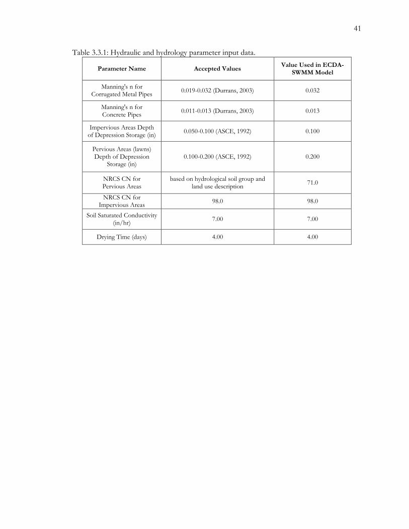
41

Table 3.3.1: Hydraulic and hydrology parameter input data.

Parameter Name Accepted Values Value Used in ECDA-

SWMM Model

Manning's n for Corrugated Metal Pipes

0.019-0.032 (Durrans, 2003) 0.032

Manning's n for Concrete Pipes

0.011-0.013 (Durrans, 2003) 0.013

Impervious Areas Depth of Depression Storage (in)

0.050-0.100 (ASCE, 1992) 0.100

Pervious Areas (lawns) Depth of Depression

Storage (in) 0.100-0.200 (ASCE, 1992) 0.200

NRCS CN for Pervious Areas

based on hydrological soil group and land use description

71.0

NRCS CN for Impervious Areas

98.0 98.0

Soil Saturated Conductivity (in/hr)

7.00 7.00

Drying Time (days) 4.00 4.00

42

Chapter 4

RESULTS AND ANALYSIS

4.1 Precipitation Data

During the one-year analysis period of this study (2007), 33.8 in. of total rainfall data

were cataloged at the University Weather Station on the Main Campus Watershed. Table

4.1.1 shows the monthly percent difference between the 100-year average rainfall data and

the observed rainfall data of 2007. For the 2007 data, rainfall in the Main Campus

Watershed was 11.9% less than the 100-year average, including differences in rainfall of -

50.9% in May and -40.7% in September. This less-than-average rainfall in the fall of 2007

prompted the Department of Environmental Protection to declare a drought watch in most

of the Commonwealth of Pennsylvania, including Centre County (DEP, 2007; Dvorak,

2007).

Table 4.1.1: 1882-1990 average monthly precipitation for State College, PA, average monthly observed data for 2007, and the percent difference.

Month 2007 Observed

Rainfall (in.) 100-year Average Rainfall data (in.)

Percent Difference relative to the 100-year Average Rainfall Data (%)

January 2.12 2.74 -22.6

February 1.14 2.54 -55.1

March 2.94 3.34 -12.0

April 3.45 3.30 4.55

May 1.95 3.97 -50.9

June 2.61 4.01 -34.9

July 3.32 3.74 -11.2

August 4.55 3.40 33.8

September 1.76 2.97 -40.7

October 2.35 2.86 -17.8

November 3.85 2.85 35.1

December 3.80 2.67 42.3

Total 33.8 38.4 -11.9

43

The decrease in precipitation in 2007 in the Main Campus Watershed was

accompanied by a lesser number of larger volume rain events and also decreased the amount

of higher intensity storm events. The 2007 rainfall data were broken into 122 precipitation

events in which 46 of the rainfall events had less than 0.05 in. of rain total. Precipitation

events of less than 1/20th of an inch (0.060 in.) rarely generate runoff, meaning that for this

study, only the 76 events that produced 0.060 in. of rain or greater were studied and analyzed

(Zhang and Hamlett, 2006).

Intensity-duration-frequency (IDF) curves for State College were produced using

current data available at the National Oceanic and Atmospheric Administration (NOAA)

website (NOAA, 2008). The probabilistic relationship between the precipitation duration,

rainfall intensity, storm return periods and the 76 precipitation events are represented

graphically in Figure 4.1.1. The 76 precipitation events then were broken down to 1-, 2-, 5-,

10-, 25-, and 100-year period events. As Figure 4.1.1 depicts, in 2007, the largest return

event was a 1-year precipitation event and, therefore, all the rest of the 75 rainfall events are

below the 1-year event curve.

Figure 4.1.1: Intensity Duration Frequency Curves (IDF) for State College, PA,

with the 76 precipitation events larger than 0.05 in. rainfall depth that fell in 2007 on the Main Campus Watershed (NOAA, 2008).

0.001

0.01

0.1

1

10

10 100 1000

Rai

nfa

ll In

ten

sity

(in

/hr)

Rainfall Duration (minutes)

100-yr50-yr25-yr10-yr

5-yr2-yr1-yr

1-year

44

4.2 Validation of the Rainfall Runoff Storm Event Data

The measured stormwater discharge, collected from the cloverleaf outlet structure,

was plotted under rainfall hyetographs in order to verify the data to make sure the observed

timing of runoff data matched the timing of the rainfall data. Figure 4.2.1 shows that the

timing of the stormwater peak runoff flow for the 7/11/07 storm event matches the timing

of the highest 5-minute intensities of the rainfall events. This visual validation of the storm

events data was implemented for all the storm events prior to calibration, which will be

discussed in greater detail in the next section.

Figure 4.2.1: ECDA observed rainfall validation: Rainfall hyetograph versus

observed runoff for the 7/11/07 storm event.

0

0.2

0.4

0.6

0.8

1

1.2

0

0.05

0.1

0.15

0.2

0.25

0.3

0.35

0.4

0.45

Accu

mu

lative R

ainfall (in

.)

5-M

inu

te R

ain

fall

(in

.)

0

5

10

15

20

25

30

35

7/1

1/0

7 1

3:0

0

7/1

1/0

7 1

3:3

0

7/1

1/0

7 1

4:0

0

7/1

1/0

7 1

4:3

0

7/1

1/0

7 1

5:0

0

7/1

1/0

7 1

5:3

0

7/1

1/0

7 1

6:0

0

7/1

1/0

7 1

6:3

0

7/1

1/0

7 1

7:0

0

7/1

1/0

7 1

7:3

0

7/1

1/0

7 1

8:0

0

7/1

1/0

7 1

8:3

0

7/1

1/0

7 1

9:0

0

7/1

1/0

7 1

9:3

0

7/1

1/0

7 2

0:0

0

Flo

w R

ate

(cfs

)

45

4.3 ECDA-SWMM Model Development Results

4.3.1 ECDA-SWMM Sensitivity Analysis

A sensitivity analysis was performed in order to evaluate the significance of each

modeling parameter. The 6/22/06 and 6/23/06 storm events were used to systematically

determine which model parameters have a significant effect on the surface runoff. For this

analysis, a significant effect means that if a certain parameter was adjusted by ± 100%, the

output results would show changes greater than ± 5%. The sensitivity analysis results for

the two storms were almost identical and therefore validated the use of the sensitivity

analysis for multiple storm events. Figures 4.3.1 and 4.3.2 show the sensitivity of the runoff

volume and runoff peak flow results to various percentage changes in the parameters for the

6/22/06 event. The sensitivity analysis examined the following parameters: percent of non-

building imperviousness, impervious depression storage depth, pervious depression storage

depth, slope, width of overland flow, percent of impervious area with no depression storage,

pipe roughness coefficient, soil saturated conductivity, and curve number. The sensitivity

analysis was performed by adjusting each parameter by +/- 25%, 50%, 75% and 100%.

Parameters not shown in Figures 4.3.1 or 4.3.2 including the curve number, soil saturated

conductivity, and pervious depression storage depth, were also analyzed. These parameters

did not show significant changes in the model outputs. Although these parameters were

adjusted the maximum of ± 100%, the peak flows and runoff volumes in the ECDA-

SWMM model simulation results were not affected greater than ± 5%, which was this

study‟s parameter for determining significant effects. The curve number is typically the

parameter which has the greatest impact on peak volume rates in a sensitivity analysis;

however, it did not have a significant effect on the ECDA-SWMM model because the

ECDA is a highly urbanized catchment area with a high impermeability percentage (Davis et

46

al., 2006). Possibly, the curve number did not influence the model‟s results because the two

storms that were used for the sensitivity analysis were both moderate rainfall events resulting

in minimal runoff. Similarly, the soil saturated conductivity and pervious depression storage

depth both are associated with infiltration and therefore do not play an influential role in the

ECDA-SWMM model because of its high imperviousness (Nix, 1994).

Figure 4.3.1: Pre-calibration peak runoff sensitivity analysis of the

ECDA-SWMM model using the 6/22/06 storm event.

The pre-calibration peak runoff sensitivity analysis shows a linear change with all of

its parameters except for the pipe roughness. Decreasing the pipe roughness parameter by

75% caused the peak runoff to decrease, while it was expected to have increased linearly. An

explanation for this decrease is feedback in one or more of the 44 pipe conduits causing the

runoff to be restricted therefore decreasing the peak runoff. Ideally, it would be possible to

change the pipe roughness one conduit at a time and then run separate simulations in order

-100%

-80%

-60%

-40%

-20%

0%

20%

40%

60%

80%

100%

-100% -75% -50% -25% 0% 25% 50% 75% 100%

Pe

rce

nt

Ch

ange

in P

eak

Ru

no

ff

Percent Change in Indicated Parameters

i = Non Building Imperviousness w = Width of Overland flow

s = Slope z = % of Impervious Area with Zero Storage

d = Impervious Depression Storage Depth p = Pipe Roughness

z

w

ds

p

i

47

to look for feedback in each pipe. Given that the model runs as a whole entity and there are

many pipes feeding into each other, finding the confining combination of interacting pipes

would be difficult.

Figure 4.3.2: Pre-calibration runoff total volume sensitivity analysis of

the ECDA-SWMM model using the 6/22/06 storm event.

The sensitivity analysis in Figure 4.3.1 depicts that the peak runoff is most sensitive

to changes in non-building imperviousness, width of overland flow, slope, and pipe

roughness coefficient. Figure 4.3.2 shows that the ECDA-SWMM model runoff volume

results are most sensitive to changes with the non-building imperviousness parameter and

the impervious depression storage depth parameter. These were the same parameters that

were most sensitive in a SWMM model study done by Barco et al. (2008). The four

parameters that were used in the next section to calibrate the ECDA-SWMM model are the

non-building imperviousness, impervious depression storage depth, slope and width of

-100%

-80%

-60%

-40%

-20%

0%

20%

40%

60%

80%

100%

-100% -75% -50% -25% 0% 25% 50% 75% 100%

Pe

rce

nt

Ch

ange

in R

un

off

Vo

lum

e

Percent Change in Indicated Parameters

I = Non Building Imperviousness d = Impervious Depression Storage Depth

i

d

48

overland flow. These results from the sensitivity analysis allowed a more systematic and

focused approach to the calibration of the ECDA-SWMM model because the four

parameters that have a noteworthy effect on the model outputs are known and can be

adjusted and utilized for a specific reason (Lee et al., 2008).

4.3.2 ECDA-SWMM Model Calibration

Understanding the primary modeling objective is necessary in order to discern the

interconnection between the “path to model calibration” and the data observed. The

ECDA-SWMM modeling objective in this thesis was to successfully calibrate and simulate

between three to six storm events and come within a margin of error of ± 10% of the

observed data . In order for a model to be credible and conclusive, between three to six

storms need to be “reasonably well calibrated” (Nix, 1994). Single storm events with less

than 0.10 in. of rainfall were not simulated because this diminutive amount of precipitation

would not produce a large enough runoff peak and/or runoff volume to be constructively

evaluated (Tsihrintzis and Sidan, 2008). Data from 29 storm events with more than 0.10 in.

of rainfall were then organized and prepared to be utilized by formatting them into

precipitation input files for the ECDA-SWMM model. Next, the ECDA-SWMM model

was run to simulate the peak flows and runoff volumes for the 29 storm events. Calibration

simulations were performed on a trial-and-error basis with the 29 storm events, and five

storm events were chosen to be utilized for this study because they successfully simulated

within a range of error of ± 10% of the observed data. Appendix B.3 lists all 29 storm

events observed, uncalibrated and calibrated peak runoff, and total runoff volume data.

After calibrating all the storm events, resulting in only five out of the 29 storm

events falling within a range of error of ± 10% of the observed data, the ECDA-SWMM

model demonstrated that it is not a generally fair representation of the observed data.

49

Although this may be significant in other studies, the model is not being used here to predict

the accuracy of future storm events; it is being used as a vehicle to simulate future

generalized RWH scenarios.

For a visualization of the divergence between observed and simulated results, the

calibrated and observed peak and total runoff then were normalized by dividing each

simulation run by its observed counterpart. See Appendix B.4 for the results of all 29 storm

events. Figure 4.3.3 presents normalized data (i.e. simulated/observed) in a graphical form.

Data for the five selected storm events are presented as calibrated and non-calibrated

normalized points as a function of total rainfall. The remaining 24 storm events are

presented as calibrated and non-calibrated normalized points as a function of total rainfall.

Running averages of the 24 storm events not selected for this analysis show a non-linear

relationship between rainfall and model accuracy; however, this running average illustrates

that the general positive effect of calibration on all 29 storm events. The next section of this

chapter first will show the uncalibrated simulation of the five uncalibrated storm events

selected and then compare the deviation with the rest of the 29 simulated storm events.

4.3.3 Uncalibrated Simulations for Five Selected Storm Events

The uncalibrated simulations for the five selected storm events were run using the

ECDA-SWMM model and then the predicted outputs were compared to the observed total

runoff volume, the runoff peaks, and the runoff peak timing. Figure 4.3.4 (a-e) on page 51

shows that the simulated peak runoff timing for the five simulated storm events agrees well

with the observed peak flow. The simulations also show that in all five storm events, the

simulations over-predict the peak rates and quantity of the runoff.

50

Fig

ure

4.3

.3: N

orm

aliz

ed p

eak r

un

off

an

d n

orm

aliz

ed t

ota

l vo

lum

e ru

no

ff f

or

all 29 s

torm

s.

51

(a) 06/22/06 (b) 06/27/06

(c) 07/12/06(2) (d) 07/22/06(1)

(e) 06/08/07

Figure 4.3.4: ECDA-SWMM uncalibrated simulations for five selected storm events.

0

0.1

0.2

0.3

0.4

0.5

0.6

0.7

0.80

10

20

30

40

50

60

70

6/2

2/0

6 1

9:0

0

6/2

2/0

6 1

9:3

0

6/2

2/0

6 2

0:0

0

6/2

2/0

6 2

0:3

0

6/2

2/0

6 2

1:0

0

6/2

2/0

6 2

1:3

0

6/2

2/0

6 2

2:0

0

6/2

2/0

6 2

2:3

0

6/2

2/0

6 2

3:0

0

6/2

2/0

6 2

3:3

0

6/2

3/0

6 0

:00

Rai

nfa

ll (i

n.)

Flo

w R

ate

(cf

s)

Time

0

0.1

0.2

0.3

0.4

0.5

0.6

0.7

0.80

10

20

30

40

50

60

70

6/2

7/0

6 1

3:0

0

6/2

7/0

6 1

4:0

0

6/2

7/0

6 1

5:0

0

6/2

7/0

6 1

6:0

0

6/2

7/0

6 1

7:0

0

6/2

7/0

6 1

8:0

0

6/2

7/0

6 1

9:0

0

6/2

7/0

6 2

0:0

0

6/2

7/0

6 2

1:0

0

6/2

7/0

6 2

2:0

0

6/2

7/0

6 2

3:0

0

6/2

8/0

6 0

:00

Rai

nfa

ll (i

n.)

Flo

w R

ate

(cf

s)

Time

0

0.1

0.2

0.3

0.4

0.5

0.6

0.7

0.80

5

10

15

20

25

7/1

2/0

6 1

7:0

0

7/1

2/0

6 1

7:3

0

7/1

2/0

6 1

8:0

0

7/1

2/0

6 1

8:3

0

7/1

2/0

6 1

9:0

0

7/1

2/0

6 1

9:3

0

7/1

2/0

6 2

0:0

0

7/1

2/0

6 2

0:3

0

7/1

2/0

6 2

1:0

0R

ain

fall

(in

.)

Flo

w R

ate

(cf

s)

Time

0

0.1

0.2

0.3

0.4

0.5

0.6

0.7

0.80

5

10

15

20

25

30

35

40

45

7/2

2/0

6 7

:00

7/2

2/0

6 7

:30

7/2

2/0

6 8

:00

7/2

2/0

6 8

:30

7/2

2/0

6 9

:00

7/2

2/0

6 9

:30

7/2

2/0

6 1

0:0

0R

ain

fall

(in

.)

Flo

w R

ate

(cf

s)

Time

0

0.1

0.2

0.3

0.4

0.5

0.6

0.7

0.80

5

10

15

20

25

6/8

/07

19

:00

6/8

/07

19

:30

6/8

/07

20

:00

6/8

/07

20

:30

6/8

/07

21

:00

6/8

/07

21

:30

6/8

/07

22

:00

6/8

/07

22

:30

6/8

/07

23

:00

6/8

/07

23

:30

6/9

/07

0:0

0R

ain

fall

(in

.)

Flo

w R

ate

(cf

s)

Time

52

4.3.4 ECDA-SWMM Uncalibrated Error Analysis

The flow peak and total volume error were calculated using the normalized

percentage error (NPE) using the following equation:

𝑁𝑃𝐸𝑋𝑖=

𝑋𝑠𝑖−𝑋𝑜𝑖

𝑋𝑜𝑖

∗ 100 (Eq. 4.3.1)

where X is either the peak runoff (Qp) or the total runoff volume (VT); the subscripts s and o

indicate whether observed quantities are simulated or observed, and the subscript i is a

numerical index meaning the ith storm. The NPE of the five storm events then was

compared to the mean normalized percentage error (MNPE) of all 29 storm events with

more than 0.10 in. of rainfall using the following equation:

𝑀𝑁𝑃𝐸𝑋 =1

𝑀 𝑁𝑃𝐸𝑋𝑖

𝑀𝑖=1 (Eq. 4.3.2)

where M is the number of storms simulated (Tsihrintzis and Sidan, 2008).

The results of all five selected storm simulations and their associated rainfall, NPE

error, and MNPE error characteristics are shown in Table 4.3.1; Appendix B.5 shows the

results from the 29 storm events. Storm events with a one or two in the parenthesis were

multiple peaking storm events that were split up in order to isolate peak runoff flows. The

multiple peaking storm events were analyzed as separate storm events only if they had a gap

of no rain greater than three hours.

Table 4.3.1: Summary of the five uncalibrated storm events.

Storm Event Total

Rainfall (in.) Uncalibrated VT NPE (%)

Uncalibrated Qp NPE (%)

6/22/06 0.50 86.3 68.6

6/27/06 1.52 73.6 81.7

7/12/06(2) 0.26 108 128

7/22/06 (1) 0.38 106 132

6/8/07 0.32 204 269

MNPEX (%) 116 136

53

The five uncalibrated storm events selected had a MNPE error of 116% (VT) and

136% (Qp), compared with the 29-storm MNPE error of 168% (VT) and 197% (Qp). The

over-simulation by the ECDA-SWMM model compels limitations to the precision of the

model or the accuracy of the data observed. In order to check the validity of the simulated

volume results of the storm events, the theoretical physical maximum amount of runoff

volume was calculated using Equation 4.3.3:

𝑀𝑎𝑥𝑖𝑚𝑢𝑚 𝑇𝑜𝑡𝑎𝑙 𝑅𝑢𝑛𝑜𝑓𝑓 𝑉𝑜𝑙𝑢𝑚𝑒 = 𝑇𝑜𝑡𝑎𝑙 𝑅𝑎𝑖𝑛𝑓𝑎𝑙𝑙 ∗ 𝐷𝑟𝑎𝑖𝑛𝑎𝑔𝑒 𝐴𝑟𝑒𝑎 (Eq. 4.3.3)

Using the Maximum Total Runoff Volume for all 29 storms, the Observed Runoff

Coefficient Ko and the Simulated Runoff Coefficient Ks were calculated using the following

equations:

𝑂𝑏𝑠𝑒𝑟𝑣𝑒𝑑 𝑅𝑢𝑛𝑜𝑓𝑓 𝐶𝑜𝑒𝑓𝑓𝑖𝑐𝑖𝑒𝑛𝑡(𝐾𝑂) =1

𝑀

𝑂𝑏𝑠𝑒𝑟𝑣𝑒𝑑 𝑇𝑜𝑡𝑎𝑙 𝑅𝑢𝑛𝑜𝑓𝑓 𝑉𝑜𝑙𝑢𝑚𝑒𝑖𝑀𝑎𝑥𝑖𝑚𝑢𝑚 𝑇𝑜𝑡𝑎𝑙 𝑅𝑢𝑛𝑜𝑓𝑓 𝑉𝑜𝑙𝑢𝑚𝑒𝑖

𝑀

𝑖

(Eq. 4.3.4)

𝑆𝑖𝑚𝑢𝑙𝑎𝑡𝑒𝑑 𝑅𝑢𝑛𝑜𝑓𝑓 𝐶𝑜𝑒𝑓𝑓𝑖𝑐𝑖𝑒𝑛𝑡(𝐾𝑆) =1

𝑀

𝑆𝑖𝑚𝑢𝑙𝑎𝑡𝑒𝑑 𝑇𝑜𝑡𝑎𝑙 𝑅𝑢𝑛𝑜𝑓𝑓 𝑉𝑜𝑙𝑢𝑚𝑒𝑖𝑀𝑎𝑥𝑖𝑚𝑢𝑚 𝑇𝑜𝑡𝑎𝑙 𝑅𝑢𝑛𝑜𝑓𝑓 𝑉𝑜𝑙𝑢𝑚𝑒𝑖

𝑀

𝑖

(Eq. 4.3.5)

where M is the number of storm events used and i implies the ith storm event.

Results for this analysis are shown in Appendix B.6. The Ks coefficient was 0.233 or

twice the Ko coefficient of 0.116. Interestingly, the results from this analysis showed that the

observed (Ko) and simulated (Ks) runoff coefficients had deviations similar to the ECDA-

SWMM normalized uncalibrated and calibrated total volume model simulations. The

average normalized uncalibrated total volume percentage for the 29 storm events was 2.68

and the average normalized calibrated total volume percentage was 1.19 (see Appendix B.4).

Both error analyses show similar deviations of the observed, uncalibrated simulations being

54

about twice as much as the simulated calibration; therefore, the accuracy of the data and the

model simulations could show limitations in this study. The model was calibrated using five

storm events that took place over a relatively brief period of time. Given the limited nature

of the data used in calibration, care should be exercised in extrapolating model simulations

beyond these data. The observed data in the 29 storms could be underestimated for the

following reasons:

The stormwater pipe network is aging and possibly leaking runoff.

The East Halls drainage network has a slope that runs in the opposite direction of

the surface topography and therefore runoff may overflow to a different drainage

area than indicated in the 2004 pipe diagrams.

The ECDA-SWMM model was constructed using CAD files from 2004 and does

not take into account any new infiltration BMPs that may have been implemented in

the last four years.

There could be an unknown number of dry wells in the ECDA that were drilled

sometime in the past that percolate stormwater directly to the baseflow or

groundwater.

The Karst topography in the area may be allowing a greater amount of the overland

flow to infiltrate more rapidly into the groundwater table.

4.3.5 Calibration Exercise and Simulations of the Five Selected Storm Events

In order for the ECDA-SWMM model to more accurately mimic the observed

watershed behavior, a calibration was performed using the appropriate parameters that were

discussed in the sensitivity analysis. The five selected storm events from Section 4.3.2 were

used in this calibration exercise. The total precipitation ranged from 1.52 in. to 0.260 in. for

55

the five selected storm events. The ECDA-SWMM model shows versatility by running

calibrations using storm events with precipitation that differed by over an inch. Also, the

ECDA-SWMM model appears capable of evaluating typical summer thunderstorms because

all five modeled storm events occurred in summer conditions during the months of June and

July. The calibration is limited to a fixed number of storms that occurred only in a fixed

number of months during the summer season. The ECDA-SWMM model calibration was

performed in the following sequence:

1) The runoff “volume” parameters were calibrated in order to best match the

simulated runoff volume to that of the observed (Nix, 1994). This was done by

adjusting the non-building imperviousness (i) and the impervious depression storage

depth (d).

2) The “peak and shape” parameters were calibrated in order to match the simulated

runoff peak to the observed. Width (w) and slope (s) were used as the parameters to

adjust the peak and shape of the hydrograph. In some cases, adjusting the peak

parameters altered the volume as well, suggesting that those parameters needed to be

readjusted until the calibrated runoff was within ± 10% of the observed data.

3) Once the calibration of one storm was completed the same process was performed

on the remaining four storm events until all five storm events were within ± 10% of

the observed peak and volume. Tables 4.3.2 though 4.3.5 show a step-by-step

process of the calibration of all five storms.

The storm event on 7/22/06 was chosen to be calibrated first because it had a

relatively low total precipitation and therefore would be more sensitive to changes in

parameters because adjusting parameters from smaller storm events causes more significant

56

changes in the results as compared to larger storm events. Table 4.3.2 shows each run

calibrated for the 7/22/06 storm event and the specific parameter that was adjusted.

Table 4.3.2: ECDA- SWMM calibration of the first storm event on 7/22/06 (1).

7/22/06 (1) - 0.38 in.

Percent of Estimated Values (%)

Run # 1 2 3 4 5 6 7 8 9

i 100 75.0 50.0 50.0 50.0 40.0 40.0 40.0 40.0

d 100 100 100 125 150 150 175 175 175

w 100 100 100 100 100 100 100 50 50

s 100 100 100 100 100 100 100 100 50

Obs. Simulated

Volume (ac-ft) 0.730 1.51 1.26 1.02 0.953 0.895 0.807 0.747 0.699 0.672

Peak (cfs) 16.8 39.0 32.3 25.5 25.0 24.5 21.7 20.7 18.5 17.2

NPE VT (%) 106 73.2 39.9 30.6 22.6 10.6 2.33 -4.25 -7.95

NPE Qp (%) 132 92.3 51.7 48.8 45.9 29.3 23.56 10.37 2.48

The first run is the starting point of this exercise and is the uncalibrated simulation

for the 7/22/06 storm event. In runs #2, #3, and #6 the non-building imperviousness was

decreased by 60% in order to decrease the total runoff volume, because according to the

sensitivity analysis the ECDA-SWMM runoff volume was most sensitive to this parameter.

The non-building imperviousness can be decreased this much (i.e., 60%) in the model

calibration because it can be argued that some non-building impervious surfaces are not

directly connected to the stormwater network. For example, some impervious surfaces such

as sidewalks, impervious sport areas and some roads and parking lots allow stormwater to

overflow onto pervious surfaces. The next variable that was adjusted was the impervious

depression storage parameter. In modeling runs #4, #5, #7 the depression storage was

increased by 75% to a value of 0.175. After run #7, the NPE total volume (VT) had

decreased to a mere 2.33% over the observed data; however, the NPE peak flow (Qp) still

had not reached an acceptable level of within ± 10%, so the width and slope parameters

were chosen to calibrate the model. These two parameters are more abstract because they

57

are difficult to measure and therefore are excellent parameters to use in the calibration (Nix,

1984). After run #9, the 7/22/06 storm event had been calibrated to a deviation of less

than ± 10% and therefore the next storm event then was able to be calibrated.

The same calibrated parameter values that were used in run #9 on the 7/22/06

storm event then were used to simulate the storm event on 6/22/06 in run #10. After

calibrating the remaining parameters with this storm in runs #10 through #13, the updated

parameters (depression storage (d) decreased to 150%, and width (w) increased to 60%)

allowed the model to effectively simulate the other four storm events within ± 10% of the

observed data. Tables 4.3.3 through 4.3.5 present the calibration sequence for the

remaining three storm events. Table 4.3.6 presents the summary of the calibrated simulation

results for the five storm events that were analyzed.

Table 4.3.3: ECDA- SWMM calibration of the 6/22/06 and 7/22/06 (1) storm events. 6/22/06 - 0.5 in. 7/22/06 (1) - 0.38 in.

Percent of Estimated Values (%)

Percent of Estimated Values (%)

Run # 10 11 12 13 Run # 14

I 40.0 40.0 40.0 40.0 i 40.0

D 175 150 150 150 d 150

w 50.0 50.0 40.0 60.0 w 60.0

s 50.0 50.0 50.0 50.0 s 50.0

Obs. Simulated Obs. Simulated

Volume (ac-ft) 1.27 1.24 1.18 1.22 1.26 Volume (ac-ft) 0.730 0.738

Peak (cfs) 40.7 34.6 33.6 33.1 36.3 Peak (cfs) 16.8 18.8

NPE VT (%) -2.43 -7.06 -4.16 -0.940 NPE VT (%) 1.10

NPE Qp (%) -15.0 -17.4 -18.6 -9.96 NPE Qp (%) 11.9

Figure 4.3.5 shows the hydrographs for all five calibrated storms events. In

comparison to Figure 4.3.4, the calibrated storm events greatly decreased the modeled total

runoff volume and runoff peak rate to within an error of ±10%. While doing so, the

stormwater peak timing seemed to have become less accurate. Nevertheless, the ECDA-

SWMM model still was able to predict and simulate the peak timing within 15 minutes. Also,

58

the timing of the observed peak flows slightly preceded the timing of rainfall. This is

possible since the recording rain gage is located outside of the ECDA watershed, thereby

experiencing rain at a different time than within the ECDA watershed.

Table 4.3.4: ECDA- SWMM calibration of the 6/27/06 and 7/12/06 (2) storm events. 6/27/06 - 1.52 in. 7/12/06 (2) - 0.26 in.

Percent of Estimated

Values (%) Percent of Estimated

Values (%) Run # 15 Run # 16

i 40.0 i 40.0

d 150 d 150

w 60.0 w 60.0

s 50.0 s 50.0

Obs. Simulated Obs. Simulated

Volume (ac-ft)

4.38 4.69 Volume (ac-ft)

0.460 0.404

Peak (cfs) 31.2 33.0 Peak (cfs) 7.06 6.41

NPE VT (%) 7.05 NPE VT (%) -12.2

NPE Qp (%) 5.92 NPE Qp (%) -9.22

Table 4.3.5: ECDA- SWMM Table 4.3.6: Summary of the five calibrated calibration of the 6/8/07 storm events. storm event.

6/8/07 - 0.32 in.

Storm Event Total

Rainfall (in.)

Calibrated VT NPE

(%)

Calibrated Qp NPE

(%)

Percent of Estimated Values (%)

6/27/2006 1.52 7.05 5.92

6/22/2006 0.5 -9.96 -0.94 Run # 17

7/22/06 (1) 0.38 1.1 11.9

i 40

6/8/2007 0.32 4.29 -4.4

d 150

7/12/06 (2) 0.26 -12.2 -9.22

w 60

MNPEX

(%) -1.94 0.64

s 50

Obs. Simulated

Volume (ac-ft) 0.210 0.220

Peak (cfs) 5.41 5.17

NPE VT (%) 4.29

NPE Qp (%) -4.40

59

(a) 06/22/06 (b) 06/27/06

(c) 07/12/06(2) (d) 07/22/06(1)

(e) 06/08/07

Figure 4.3.5: ECDA-SWMM calibrated simulations for five selected storm events.

0

0.1

0.2

0.3

0.4

0.5

0.6

0.7

0.80

10

20

30

40

50

60

6/2

2/0

6 1

9:0

0

6/2

2/0

6 1

9:3

0

6/2

2/0

6 2

0:0

0

6/2

2/0

6 2

0:3

0

6/2

2/0

6 2

1:0

0

6/2

2/0

6 2

1:3

0

6/2

2/0

6 2

2:0

0

6/2

2/0

6 2

2:3

0

6/2

2/0

6 2

3:0

0

6/2

2/0

6 2

3:3

0

6/2

3/0

6 0

:00

Rai

nfa

ll (i

n.)

Flo

w R

ate

(cf

s)

Time

0

0.1

0.2

0.3

0.4

0.5

0.6

0.7

0.80

5

10

15

20

25

30

35

40

45

6/2

7/0

6 1

3:0

0

6/2

7/0

6 1

4:0

0

6/2

7/0

6 1

5:0

0

6/2

7/0

6 1

6:0

0

6/2

7/0

6 1

7:0

0

6/2

7/0

6 1

8:0

0

6/2

7/0

6 1

9:0

0

6/2

7/0

6 2

0:0

0

6/2

7/0

6 2

1:0

0

6/2

7/0

6 2

2:0

0

6/2

7/0

6 2

3:0

0

6/2

8/0

6 0

:00

Rai

nfa

ll (i

n.)

Flo

w R

ate

(cf

s)

Time

0

0.1

0.2

0.3

0.4

0.5

0.6

0.7

0.80

5

10

15

20

25

7/1

2/0

6 1

7:0

0

7/1

2/0

6 1

7:3

0

7/1

2/0

6 1

8:0

0

7/1

2/0

6 1

8:3

0

7/1

2/0

6 1

9:0

0

7/1

2/0

6 1

9:3

0

7/1

2/0

6 2

0:0

0

7/1

2/0

6 2

0:3

0

7/1

2/0

6 2

1:0

0R

ain

fall

(in

.)

Flo

w R

ate

(cf

s)

Time

0

0.1

0.2

0.3

0.4

0.5

0.6

0.7

0.80

5

10

15

20

25

7/2

2/0

6 7

:00

7/2

2/0

6 7

:30

7/2

2/0

6 8

:00

7/2

2/0

6 8

:30

7/2

2/0

6 9

:00

7/2

2/0

6 9

:30

7/2

2/0

6 1

0:0

0R

ain

fall

(in

.)

Flo

w R

ate

(cf

s)

Time

0

0.1

0.2

0.3

0.4

0.5

0.6

0.7

0.80

2

4

6

8

10

6/8

/07

19

:00

6/8

/07

19

:30

6/8

/07

20

:00

6/8

/07

20

:30

6/8

/07

21

:00

6/8

/07

21

:30

6/8

/07

22

:00

6/8

/07

22

:30

6/8

/07

23

:00

6/8

/07

23

:30

6/9

/07

0:0

0R

ain

fall

(in

.)

Flo

w R

ate

(cf

s)

Time

60

Figure 4.3.6: Calibrated simulation peak and total volume runoff versus observed peak and

total volume runoff for the 5 storm events.

Figure 4.3.6 shows that the calibration regression for the five storm events analyzed

had a coefficient of determination (r2) of 0.970 for the peak runoff and 0.990 for the total

volume. By having r2 values so close to 1.00, the relationship between the observed and

simulated variables shows small variability and therefore the ECDA-SWMM model

simulations are statistically well representative of the observed values.

4.4 Analysis of Three Scenarios Using the ECDA-SWMM Model

Scenario 1: Current State Scenario With the use of RWH: The watershed was represented by

incorporating the utilization of 100% potential RWH. The ECDA-SWMM model was used

to simulate the effect on stormwater runoff due to a decrease in effective impervious area

through the use of rainwater catchment systems represented by SWMM storage nodes.

Scenario 2: Future Climate Change Scenario With and Without RWH: This scenario

incorporated current features (i.e., parking lots, etc.) and simulated climate change and the

predicted future increases in precipitation by inputting a greater total rainfall amount in the

y = 0.970xR² = 0.970

0

10

20

30

40

50

0 10 20 30 40 50

Sim

ula

ted

Pe

ak R

un

off

(cf

s)

Observed Peak Runoff (cfs)

y = 1.060xR² = 0.990

0

1

2

3

4

5

0 1 2 3 4 5

Sim

ula

ted

To

tal V

olu

me

(ac

re-f

t)

Observed Total Volume (acre-ft)

61

calibrated storm events within the ECDA-SWMM model. The RWH scenario then was run

with the increased rainfall storm events in order to test whether RWH was able to mitigate

the effects caused by climate change and the resulting stormwater runoff.

Scenario 3: Pre-Colonial Scenario: The watershed was considered pristine and undeveloped

with wooded groundcover and permeable soils.

4.4.1 Scenario 1: Current State Scenario With the use of RWH

Through the use of RWH, this scenario illustrates the sustainable benefits Penn State

could gain if it was to incorporate RWH systems in the ECDA. Two of these benefits

include improved stormwater management (i.e. decrease in peak flow, total runoff volume)

and the conservation of potable water. To begin with, rainwater was selected to be collected

and supplement only non-potable water in this analysis because more complex RWH

systems (i.e., systems that utilize rainwater for drinking) are more difficult and expensive to

implement. For the ECDA RWH scenario, the only non-potable uses considered include

toilet flushing and landscape irrigation. In order to determine the RWH potential, the

hydrologic potential must be compared to the water demand (Hicks, 2008).

ECDA Water Usage Analysis

A proper analysis of the water usage in the ECDA is an important component to

modeling the use of RWH. Each building on campus is equipped with its own separate water

meter to maintain an accurate account of the water used in gallons. The 2005-2007 average

total water consumption in the ECDA was 2.29 MG/day and accounted for 13% of the total

water used at Penn State(PSU, 2006; PSU, 2007b; PSU, 2008a);. Penn State is in many ways

like a small town, meaning that there are different types of buildings with different design

codes for water usage. Furthermore, water demand varies with the type of building, and

62

therefore buildings in the ECDA were categorized by sector in order to determine the

amount of water used for flushing toilets and landscape irrigation. The types of buildings in

the ECDA include academic and research buildings, sports facilities, common facilities and

student residential housing. The percentages of each building sector are shown below in

Figure 4.4.1, with academic and research buildings making up the largest percentage of

buildings in the ECDA (i.e., 47%).

Figure 4.4.1: Percent of building types in ECDA.

Figure 4.4.2 shows that the largest water-consuming buildings are residence halls,

which consume more than 50% of all the potable water in the ECDA.

Figure 4.4.2: Percent of water usage by building sector in the ECDA.

Even though water usage data was provided for each building on the ECDA, the

percentage of water used for potable and non-potable sources is not measured separately at

Academic and Research

Buildings, 47%Residence Halls, 21%

Commons Facilities, 11%

Sports Facilities, 22%

Academic and Research

Buildings, 18%

Residence Halls, 54%

Commons Facilities, 13%

Sports Facilities, 14%

63

Penn State. Therefore, the percentage of water used for non-potable uses was estimated to

be 86% for commercial buildings and 78% for domestic buildings based on previous

research (AWWARF, 1999; PI, 2003). For this analysis, the common facilities, sports

facilities, and academic and research buildings were grouped together in order to for them to

have water consumption characteristics similar to typical commercial facilities, and

residential hall water usage were selected to behave comparably to that of typical residential

structures. The water end use of a commercial building might vary in some cases. For

example, a sport facility might use more water for irrigation, yet an academic and research

building could utilize more water for toilet flushing, but since both end uses were grouped as

non-potable, there is no conflict in their being grouped in the same sector. A water

assessment case study performed by Stanford University found that toilet flushing and

landscape irrigation can account for over 30% of the water used on a college campus (SU

and MWM, 2003).

Figure 4.4.3 shows the 100% potential monthly RWH yield in comparison with the

3-year average monthly water usage. Hypothetically, if the ECDA was able to collect 100%

of the rainwater that fell on building rooftops, then it would be possible to supplement

between 14-46% of the drinking water demand and utilize rainwater for 100% of flushing

and irrigational needs. The higher end drinking water demand of 46% is well below the

selected non-potable water usage for commercial and domestic buildings of about 80%.

It is only possible to collect 100% of rooftop rainfall by designing building-specific

cisterns of adequate volume. With the water supply/demand data of the buildings on the

ECDA, an analysis of the hydrological stormwater impact and potential is explained in the

next section.

64

Figure 4.4.3: ECDA RWH yield versus water usage based on averaged monthly precipitation.

ECDA-SWMM Model Simulation with 100% RWH Potential

The five storm events that were calibrated with the ECDA-SWMM model in

Scenario (1) were utilized to run the RWH simulation. First, the ECDA-SWMM model was

adjusted by adding storage nodes that would collect and store the flow from the separate

building nodes in order to represent the storage tanks of RWH. Since 100% of the amount

of RWH yield makes up between 14-46% of the monthly water, it was accepted that 100%

of the collected rainfall could be utilized for flushing toilets and irrigation in the ECDA

buildings each month. Therefore, the storage nodes were designed to detain 100% of the

stormwater produced from each storm event. Figure 4.4.4 shows the results of the RWH

simulation. Table 4.4.1 shows the percentage differences of total runoff and peak flow rates

between the calibrated simulation and the RH simulation.

25%14%

26% 18%26% 46% 27%

33%16% 14% 15% 18%

0

2

4

6

8

10

12

14

Jan

uar

y

Feb

uar

y

Mar

ch

Ap

ril

May

Jun

e

July

Au

gust

Sep

tem

ber

Oct

ob

er

No

vem

ber

Dec

emb

er

Mill

ion

Gal

lon

s

Month

ECDA-SWMM Monthly Rainwater Harvesting Yield (MG)

3 Year Average Monthly Water Usage (MG)

65

(a) 06/22/06 (b) 06/27/06

(c) 07/12/06(2) (d) 07/22/06(1)

(e) 06/08/07

Figure 4.4.4: ECDA-SWMM simulations with 100% RWH.

0

0.1

0.2

0.3

0.4

0.5

0.6

0.7

0.80

10

20

30

40

50

60

6/2

2/0

6 1

9:0

0

6/2

2/0

6 1

9:3

0

6/2

2/0

6 2

0:0

0

6/2

2/0

6 2

0:3

0

6/2

2/0

6 2

1:0

0

6/2

2/0

6 2

1:3

0

6/2

2/0

6 2

2:0

0

6/2

2/0

6 2

2:3

0

6/2

2/0

6 2

3:0

0

6/2

2/0

6 2

3:3

0

6/2

3/0

6 0

:00

Rai

nfa

ll (i

n.)

Flo

w R

ate

(cf

s)

Time

0

0.1

0.2

0.3

0.4

0.5

0.6

0.7

0.80

5

10

15

20

25

30

35

40

45

6/2

7/0

6 1

3:0

0

6/2

7/0

6 1

4:0

0

6/2

7/0

6 1

5:0

0

6/2

7/0

6 1

6:0

0

6/2

7/0

6 1

7:0

0

6/2

7/0

6 1

8:0

0

6/2

7/0

6 1

9:0

0

6/2

7/0

6 2

0:0

0

6/2

7/0

6 2

1:0

0

6/2

7/0

6 2

2:0

0

6/2

7/0

6 2

3:0

0

6/2

8/0

6 0

:00

Rai

nfa

ll (i

n.)

Flo

w R

ate

(cf

s)

Time

0

0.1

0.2

0.3

0.4

0.5

0.6

0.7

0.80.0

1.5

3.0

4.5

6.0

7.5

9.0

7/1

2/0

6 1

7:0

0

7/1

2/0

6 1

7:3

0

7/1

2/0

6 1

8:0

0

7/1

2/0

6 1

8:3

0

7/1

2/0

6 1

9:0

0

7/1

2/0

6 1

9:3

0

7/1

2/0

6 2

0:0

0

7/1

2/0

6 2

0:3

0

7/1

2/0

6 2

1:0

0R

ain

fall

(in

.)

Flo

w R

ate

(cf

s)

Time

0

0.1

0.2

0.3

0.4

0.5

0.6

0.7

0.80

5

10

15

20

25

7/2

2/0

6 7

:00

7/2

2/0

6 7

:30

7/2

2/0

6 8

:00

7/2

2/0

6 8

:30

7/2

2/0

6 9

:00

7/2

2/0

6 9

:30

7/2

2/0

6 1

0:0

0R

ain

fall

(in

.)

Flo

w R

ate

(cf

s)

Time

0

0.1

0.2

0.3

0.4

0.5

0.6

0.7

0.80

2

4

6

8

10

6/8

/07

19

:00

6/8

/07

19

:30

6/8

/07

20

:00

6/8

/07

20

:30

6/8

/07

21

:00

6/8

/07

21

:30

6/8

/07

22

:00

6/8

/07

22

:30

6/8

/07

23

:00

6/8

/07

23

:30

6/9

/07

0:0

0R

ain

fall

(in

.)

Flo

w R

ate

(cf

s)

Time

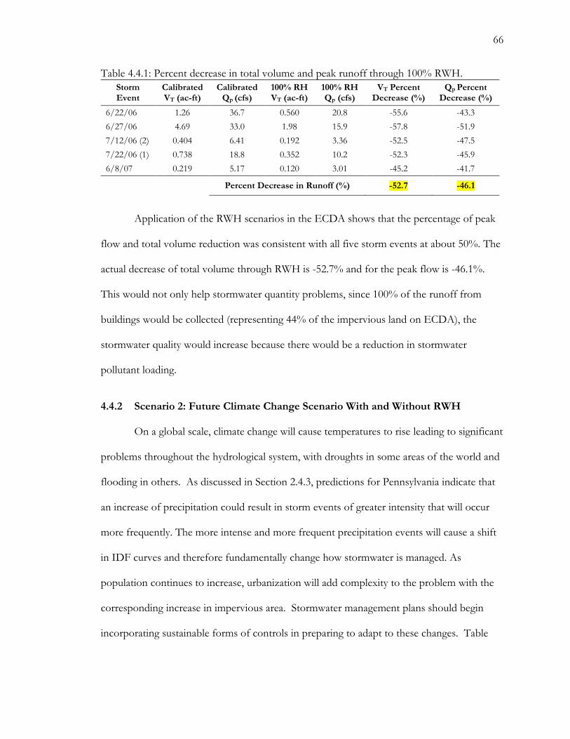
66

Table 4.4.1: Percent decrease in total volume and peak runoff through 100% RWH.

Storm Event

Calibrated VT (ac-ft)

Calibrated Qp (cfs)

100% RH VT (ac-ft)

100% RH Qp (cfs)

VT Percent Decrease (%)

Qp Percent Decrease (%)

6/22/06 1.26 36.7 0.560 20.8 -55.6 -43.3

6/27/06 4.69 33.0 1.98 15.9 -57.8 -51.9

7/12/06 (2) 0.404 6.41 0.192 3.36 -52.5 -47.5

7/22/06 (1) 0.738 18.8 0.352 10.2 -52.3 -45.9

6/8/07 0.219 5.17 0.120 3.01 -45.2 -41.7

Percent Decrease in Runoff (%) -52.7 -46.1

Application of the RWH scenarios in the ECDA shows that the percentage of peak

flow and total volume reduction was consistent with all five storm events at about 50%. The

actual decrease of total volume through RWH is -52.7% and for the peak flow is -46.1%.

This would not only help stormwater quantity problems, since 100% of the runoff from

buildings would be collected (representing 44% of the impervious land on ECDA), the

stormwater quality would increase because there would be a reduction in stormwater

pollutant loading.

4.4.2 Scenario 2: Future Climate Change Scenario With and Without RWH

On a global scale, climate change will cause temperatures to rise leading to significant

problems throughout the hydrological system, with droughts in some areas of the world and

flooding in others. As discussed in Section 2.4.3, predictions for Pennsylvania indicate that

an increase of precipitation could result in storm events of greater intensity that will occur

more frequently. The more intense and more frequent precipitation events will cause a shift

in IDF curves and therefore fundamentally change how stormwater is managed. As

population continues to increase, urbanization will add complexity to the problem with the

corresponding increase in impervious area. Stormwater management plans should begin

incorporating sustainable forms of controls in preparing to adapt to these changes. Table

67

4.4.2 shows the summary of the literature review of climate change and its effect on

precipitation in Pennsylvania.

Table 4.4.2: Predicted range of climate change impacts in Pennsylvania relative to current historical averages (see Chapter 2 of this thesis) (UCS, 2008; CIER, 2008).

2020s

(2010-2039) 2050s

(2040-2069) 2080s

(2070-2099)

Change in Average Annual Temperature

2.5° F increase

4.0-5.5° F increase

5.0-8.5° F increase

Change in Maximum Summer Temperature

2-3° F increase

2.0-7.0° F increase

3.0-12° F increase

Change in Average Annual Rainfall

5.0% increase

5.0-12% increase

12-20% increase

Change in Average Annual Snowfall

50% decrease

50-100% decrease

75-100% decrease

The main objective of this scenario is to examine the hydraulic impact to the urban

drainage system resulting from climate change. Simulations were performed using the five

storm events that were calibrated with the ECDA-SWMM model. For this scenario, an

increase amount of precipitation of 20% was selected in order to take into consideration the

worst case scenario in the impact of climate change on stormwater management. This

assumption was analyzed by increasing the precipitation of each storm event by 20% for the

5-minute interval rainfall data for each of the five storm events. The increase of

precipitation for the five storm events is displayed in Table 4.4.3.

Table 4.4.3: Climate change (CC) scenario 20% increase on the rainfall of the five storm events.

Storm Event

Rainfall (in.)

20% Increase in Rainfall (in.)

6/22/06 0.500 0.600

6/27/06 1.52 1.82

7/12/06 (2) 0.260 0.312

7/22/06 (1) 0.380 0.456

6/8/2007 0.320 0.384

68

In order to determine if this climate change scenario could be mitigated by RWH,

the RWH ECDA-SWMM model was run using the increased precipitation data. The runoff

hydrographs comparing the simulations of future climate change effects on precipitation

with the use of RWH (in purple) and without the use of RWH (in blue) are shown in Figure

4.4.5. The calibrated simulation from Section 4.3.2 is shown (in green) as the current

condition scenario with no increase in precipitation in order to illustrate the potential affect

climate change could have on stormwater peak runoff and total volume. Table 4.4.4 shows

the results of running the ECDA-SWMM model with this increased precipitation.

Table 4.4.4: Climate change (CC) scenario with 20% increase in precipitation.

Storm Event

Calibrated VT (ac-ft)

Calibrated Qp (cfs)

CC VT (ac-ft)

CC Qp (cfs)

VT Percent Increase (%)

Qp Percent Increase (%)

6/22/06 1.26 36.7 1.63 48.4 29.4 31.9

6/27/06 4.69 33.0 6.01 41.0 28.1 24.2

7/12/06 (2) 0.404 6.41 0.570 8.19 41.1 27.8

7/22/06 (1) 0.738 18.8 0.972 24.2 31.7 28.7

6/8/2007 0.219 5.17 0.333 8.53 52.1 65.0

Percent Increase in Runoff (%) 36.5 35.5

In the climate change scenario, the peak runoff and total volume would increase by

about 35%. Results from the simulation produced by the ECDA-SWMM model of

combining the climate change scenario‟s adjusted rainfall storm events and the RWH

scenario from section 4.4.1 are listed in Table 4.4.5, which shows the hydraulic effect RWH

would have on peak runoff and total volume discharge in storm events affected by future

climate change increases in precipitation.

RWH can be viewed as a sustainable solution to difficulties of stormwater

management in the coming years. This section reveals that even though stormwater quantity

(peak and total volume runoff) possibly could be increased by 35% because of climate

change, RWH still would be able offset this increase by decreasing total volume flows by

69

(a) 06/22/06 (b) 06/27/06

(c) 07/12/06(2) (d) 07/22/06(1)

(e) 06/08/07(1)

Figure 4.4.5: ECDA-SWMM simulations with a 20% increase in precipitation from future climate change scenarios and the mitigation of stormwater through 100% RWH.

0

0.1

0.2

0.3

0.4

0.5

0.6

0.7

0.80

10

20

30

40

50

60

6/2

2/0

6 1

9:0

0

6/2

2/0

6 1

9:3

0

6/2

2/0

6 2

0:0

0

6/2

2/0

6 2

0:3

0

6/2

2/0

6 2

1:0

0

6/2

2/0

6 2

1:3

0

6/2

2/0

6 2

2:0

0

6/2

2/0

6 2

2:3

0

6/2

2/0

6 2

3:0

0

6/2

2/0

6 2

3:3

0

6/2

3/0

6 0

:00

Rai

nfa

ll (i

n.)

Flo

w R

ate

(cf

s)

Time

0

0.1

0.2

0.3

0.4

0.5

0.6

0.7

0.805

10152025303540455055

6/2

7/0

6 1

3:0

0

6/2

7/0

6 1

4:0

0

6/2

7/0

6 1

5:0

0

6/2

7/0

6 1

6:0

0

6/2

7/0

6 1

7:0

0

6/2

7/0

6 1

8:0

0

6/2

7/0

6 1

9:0

0

6/2

7/0

6 2

0:0

0

6/2

7/0

6 2

1:0

0

6/2

7/0

6 2

2:0

0

6/2

7/0

6 2

3:0

0

6/2

8/0

6 0

:00

Rai

nfa

ll (i

n.)

Flo

w R

ate

(cf

s)

Time

0

0.1

0.2

0.3

0.4

0.5

0.6

0.7

0.80

3

6

9

12

7/1

2/0

6 1

7:0

0

7/1

2/0

6 1

7:3

0

7/1

2/0

6 1

8:0

0

7/1

2/0

6 1

8:3

0

7/1

2/0

6 1

9:0

0

7/1

2/0

6 1

9:3

0

7/1

2/0

6 2

0:0

0

7/1

2/0

6 2

0:3

0

7/1

2/0

6 2

1:0

0R

ain

fall

(in

.)

Flo

w R

ate

(cf

s)

Time

0

0.1

0.2

0.3

0.4

0.5

0.6

0.7

0.80

5

10

15

20

25

30

35

7/2

2/0

6 7

:00

7/2

2/0

6 7

:30

7/2

2/0

6 8

:00

7/2

2/0

6 8

:30

7/2

2/0

6 9

:00

7/2

2/0

6 9

:30

7/2

2/0

6 1

0:0

0R

ain

fall

(in

.)

Flo

w R

ate

(cf

s)

Time

0

0.1

0.2

0.3

0.4

0.5

0.6

0.7

0.80

2

4

6

8

10

6/8

/07

19

:00

6/8

/07

19

:30

6/8

/07

20

:00

6/8

/07

20

:30

6/8

/07

21

:00

6/8

/07

21

:30

6/8

/07

22

:00

6/8

/07

22

:30

6/8

/07

23

:00

6/8

/07

23

:30

6/9

/07

0:0

0R

ain

fall

(in

.)

Flo

w R

ate

(cf

s)

Time

70

Table 4.4.5: Climate change – RWH (CC-RWH) scenario with 20% increase in precipitation and 100% RWH potential.

Storm Event

CC VT (ac-ft)

CC Qp (cfs)

CC-RWH VT (ac-ft)

CC-RWH Qp (cfs)

VT Percent Decrease (%)

Qp Percent Decrease (%)

6/22/06 1.63 48.4 0.730 28.2 -55.2 -41.8

6/27/06 6.01 41.0 2.68 19.5 -55.5 -52.4

7/12/06 (2) 0.570 8.19 0.192 3.36 -66.3 -58.9

7/22/06 (1) 0.972 24.2 0.454 12.6 -53.3 -48.0

6/8/07 0.333 8.53 0.173 4.91 -48.0 -42.3

Percent Decrease in Runoff (%) -55.7 -48.7

-55.7% and peak flows by -48.7%. The increased runoff of the future climate change

scenario does not significantly decrease the percentage of stormwater quantity that RWH is

able to mitigate because the more stormwater produced just increases the amount of

rainwater collected and reused.

4.4.3 Scenario 3: Pre-Colonial Scenario

One goal of sustainable development is to have zero impact on the environment.

Goals of this type are seen in other environmental disciplines; for drinking water the

Maximum Contamination Level Goals for many contaminants is zero. This would be similar

to setting a goal for stormwater of zero impact from pre-construction levels by minimizing

the detrimental impacts of stormwater discharge (i.e., no temperature changes, no

sedimentation loading, no erosion damage, no increase in Biological Oxygen Demand, etc.).

When planning or evaluating a stormwater management design, it is important to quantify

the “zero” impact as a benchmark; one way that can be done is by assessing the pre-colonial

runoff and stream conditions before the impact of imperviousness. Pre-colonial conditions

represent an example of the natural flow of runoff and could be a zero discharge aspiration

to be emulated as an innovative approach to sustainable stormwater management to

minimize the environmental impact of stormwater discharge. In this section, the East

71

Campus Drainage Area‟s stormwater runoff was evaluated based on its pre-development

conditions and then modeled using the calibrated ECDA-SWMM model.

In the early 1800‟s, central Pennsylvania would have been covered by an

undeveloped pristine watershed, with permeable soils and wooded groundcover. Before the

rise of the metal industry in Pennsylvania, which caused the deforestation of much of the

region, rainwater infiltrated naturally into the ground and overflowed at lower speeds

downslope to the discharge point. This scenario was modeled as a baseline condition in

order for discussion later in this thesis regarding stormwater management goals.

In order to simulate a pre-colonial scenario, several of the calibrated ECDA-SWMM

model parameters were adjusted. First, the percentage of building and non-building

imperviousness for all 53 sub-catchments was adjusted to 0 in order to model a pre-

developed watershed without the impact that buildings, roads, sidewalks, and all other land

uses have on stormwater runoff. Next, the SCS Curve Number was lowered to 55; a value

set for heavy mixed woods and forests for all the sub-catchments in which brush covers the

ground. All five storm events then were run with these pre-colonial conditions and the

results showed that all the stormwater runoff would infiltrate giving a value of zero

discharge. Even when the 1.42 in. precipitation event on the 6/27/06 storm event was used

as the input, the ECDA-SWMM produced zero discharge.

In most cases, zero impact for drinking water is unattainable. Similarly, a zero

discharge stormwater management philosophy would be difficult to achieve but it is being

practiced as a sustainable solution to stormwater management at another drainage area on

Penn State Campus. The Fox Hollow Drainage Basin at Penn State has impervious land on

28% of the drainage area but produces runoff equal to only 3% of the annual precipitation

(PSU 2007a). This drainage basin shares a border with the ECDA and serves as the most

72

progressive basin for stormwater management at Penn State. Stormwater in the Fox Hollow

Drainage Basin is managed through the use of stormwater BMPs including an aggressive

approach to stormwater infiltration. In order for the ECDA‟s stormwater management to

become more sustainable, Penn State must begin trying to emulate the pre-colonial

conditions by reducing the amount of stormwater runoff. One way to attempt to meet a

zero discharge goal is to minimize the detrimental impact of stormwater discharge through

the use of RWH on future construction projects.

When considering the benefits of RWH the true value, which includes an economic

analysis on the ECDA, also must be considered. The next section illustrates the financial

benefits of utilizing RWH on a sample future building project.

4.5 Financial Analysis of Rainwater Harvesting

RWH systems could have significant environmental benefits by reducing stormwater

peak runoff and total volume; but in order to measure the total sustainable impact of the

collection and reuse of rainwater, tangible costs must be quantified through a financial

analysis. A “conservative” financial evaluation was performed instead of a full economic

analysis because social and environmental “non-monetary” intangibles or externalities are

discussed but are not included in the capital (Roebuck, 2007). This section evaluates three

different RWH financial analyses:

1) Retrospective Water Savings Analysis: Water savings analysis through the use of

RWH on 100% of buildings in the ECDA.

2) Present Financial Analysis: Comparison of the use of RWH on the Millennium

Science Complex (MSC) and the proposed conventional stormwater facility.

73

3) Future Financial Analysis: Use of RWH instead of green roofs on future buildings

that Penn State has proposed under the University Park Master Plan for future

campus building infrastructure projects.

4.5.1 Retrospective Water Savings Analysis

Penn State could benefit economically through lower water bills and avoided costs of

future stormwater infrastructure by having the capacity to utilize 100% of the potential

RWH within the ECDA. For this hypothetical and retrospective financial analysis, the

amount of water conserved and the savings from future water bills are analyzed. Table 4.5.1

shows the price of water and wastewater for the past five years; the rates of 2004-2005 are

missing from the data set (PSU, 2004; PSU, 2006; PSU, 2007b; PSU, 2008a). The price of

water includes the monetary value of water and also the energy used to pump the water and

wastewater. There is an increasing trend of higher water prices each year; therefore the

amount of money saved in annual water bills could be significant. The costs for the two

utilities were selected to have identical fees for each commodity because Penn State does not

separate the water and wastewater rates. Using the most current data for potable water rates

($4.19 per 1000 gallons) and assuming the 100% RWH scenario in the ECDA for a time

period of one year (refer to Table 4.4.3 for 100% RWH yield monthly values), Penn State

would save $96,135 in future water bills per year and also would conserve over 22.6 million

gallons of fresh drinking water per year. This does not take into account the following

possible intangible costs: the price of water continuing to increase, the costs of possible

future flooding events, future aging stormwater infrastructure replacement costs, or potential

stormwater permitting and mitigation costs (Roebuck, 2007).

The hypothetical situation of utilizing RWH in all the buildings in the ECDA (as

described in Scenario 1) would not be financially beneficial because the implementation of

74

Table 4.5.1: University Park, PA, water and wastewater utility rates (PSU, 2004; PSU, 2006; PSU, 2007b; PSU, 2008a).

Year Water and Wastewater

Costs (per 1000 Gallons) Price Change

Since 2003 (%)

2007-2008 $8.38 33.9%

2006-2007 $7.83 25.1%

2005-2006 $7.16 14.4%

2003-2004 $6.26 --

RWH on existing infrastructures is extremely difficult and costly due to the high price and

complexity of retrofitting RWH on every building in the ECDA. Therefore, the costs of

constructing a RWH system are discussed in terms of a real construction project that is

currently taking place at Penn State.

4.5.2 Present Financial Analysis

In September of 2008, Penn State began building the Millennium Science Complex

(MSC), located on the corner of Bigler Road and Pollock Road (see the building design

details used for this analysis in Table 4.5.2 and its precise location in Figure 4.5.1) on the

existing ECDA (Cullerot and Whelan, 2008). The current land use for the site includes

sports fields, two tennis courts and two roller hockey rinks. The new 275,600 gross square-

foot (GSF) research building (99,836 ft2 roof catchment area) will be the largest in the

ECDA. The MSC will increase the total building impermeability in the ECDA from 21.74

acres to 24.03 acres and increase the total imperviousness of the ECDA by 2%. Like all

buildings built at Penn State since 2004, the MSC is planned to be built to meet Leadership

in Energy and Environmental Design (LEED) standards and will feature a green roof in

order to reduce the stormwater impact in the ECDA. Also, an underground stormwater

detention pipe system is being built and implemented in order to meet storm design

standards.

75

Table 4.5.2: MSC building details.

Number of Stories 4

Gross Floor Area 276,000 ft2

Total Roof Catchment Area 94,400 ft2

Green Roof Catchment Area 50,000 ft2

Ground Floor Patio Garden 4220 ft2

Design Occupants 2990 people

Design Water Closets 60 toilets

Toilet Demand 1.60 Gallon/flush

Flushes/occupant 3/day

Irrigation 1.50 inches/week

Figure 4.5.1: Location of the Millennium Science Building with

the five green roofs labeled (GR).

76

Water Balance for the Millennium Science Complex

In order to calculate the RWH potential supply, a water balance estimate must be e

for the MSC. First, the monthly rainwater supply was calculated using the monthly rainfall

data for State College, PA, the MSC‟s total roof square feet (SF), and the following equation:

𝑅𝑎𝑖𝑛𝑤𝑎𝑡𝑒𝑟 𝑃𝑜𝑡𝑒𝑛𝑡𝑖𝑎𝑙 𝑆𝑢𝑝𝑝𝑙𝑦 = 𝑃𝑟𝑒𝑐𝑖𝑝𝑖𝑡𝑎𝑡𝑖𝑜𝑛 ∗ 𝐾𝑟𝑜𝑜𝑓 ∗ 𝑆𝐹 ∗ 0.623 (Eq. 4.4.1)

where 𝐾𝑟𝑜𝑜𝑓 = 0.9 because the first 10% of rainwater typically is lost to initial abstractions

such as transpiration, evaporation, and surface wetting (Hicks, 2008). The value of 0.623

was used as the precipitation unit conversion from inches of precipitation to gallons/square

foot. The toilet water usage demand for the MSC was calculated by assuming that each of

the “design building occupants” would flush a toilet three times a day at 1.6 Gallons per

flush (Hicks, 2008). The selected irrigation water usage was calculated by assuming that the

4220 ft2 garden would have a water demand of 1.5 in. of water per week (Hicks, 2008).

Figure 4.5.2 shows the comparison of the RWH supply and the total water demand for

toilets and irrigation. By collecting and utilizing 90% of the rainwater that runs off the MSC

building, between 32-50% of the potable water used for flushing toilets could be conserved.

This could result in up to $8700 of water savings per year at the current water rate of

$4.19/1000 gallons.

The MSC currently is designed to have a green roof that will cover over an acre of

the MSC‟s roof and will cost $1.25 million. Because green roofs can only “retain the first

inch” of storm events and by code the stormwater system must be able to handle a 100-year

storm event, an additional stormwater management structure must be built in order to

decrease predevelopment runoff peak and volume rates (Buranen, 2008). In front of the

MSC, a conventional subterranean stormwater pond for the management of the MSC‟s

77

Figure 4.5.2: MSC RWH 90% yield versus calculated water usage.

stormwater is being built that consists of five 240 ft long, 48 in. corrugated steel detention

pipes that run parallel to Pollock Road. This conventional stormwater detention facility was

designed ignoring the green roof‟s retention capabilities. The costs of the purchase and

installation of the corrugated steel detention pipes is compared financially to a RWH system

appropriate for the MSC. For this analysis, the Stormtank, RWH system stormwater storage

modules (Brentwood Industries, 2009) was chosen to be analyzed (See Figure 4.5.3). The

Stormtank RWH system will be able to detain the stormwater on site for landscape irrigation

and toilet flushing while also being able to handle the same volume of stormwater as the

proposed conventional stormwater structures in order to meet stormwater peak and volume

NPDES II regulations (Reidy, 2008).

33%31%

41% 40%

48% 49%46%

41%36% 35% 35% 33%

0

0.1

0.2

0.3

0.4

0.5

0.6

Jan

uar

y

Feb

uar

y

Mar

ch

Ap

ril

May

Jun

e

July

Au

gust

Sep

tem

ber

Oct

ob

er

No

vem

ber

Dec

emb

er

Mill

ion

Gal

lon

s

Month

Rainwater Harvesting Supply (MG)

Total Water Demand for Toilets and Irrigation (MG)

78

Figure 4.5.3: Schematic of the proposed MSC RWH system

(Adapted from Roebuck, 2007).

The Stormtank stormwater storage modular cells were selected for several reasons:

The modular storage cells create a 97% void space allowing them to optimize the

amount of water that can be stored in a smaller area. They are then wrapped with an

impermeable membrane to act just like an ordinary cistern or detention structure.

Each Stormtank stormwater storage modular cell can take loads up to 2.32 tons per ft2

allowing them to be built under parking lots, streets, or recreational facilities.

Maintenance costs are minimal.

In order to estimate the costs or savings associated with an integrated stormwater

management system, detailed assumptions were made based on available data sources (see

Table 4.5.3). The conventional system is designed to store up to 113,000 gallons (total

volume of five 240-ft long, 48 in. corrugated steel pipes) and the modular RWH system is

designed to collect up to 220,000 gallons (each Stormtank modular cell holds about 100

gallons). The RWH system modular detention size was estimated assuming the maximum

amount of rainfall that would need to be collected in the month with the maximum amount

of rainfall.

79

Table 4.5.3: Installation costs of RWH system and conventional stormwater system.

RWH System Unit Cost Count Total Cost

Stormtank Modular Cells (Brentwood Industries, 2009) (each cell is 36 in. * 36 in. * 18 in.)

units $67.50 2244 $151,470.00

Stormtank Plumbing (Hicks, 2008) (i.e. overflow, potable water supply, actuated valves, and tank level sensors)

each $2,541.60 1 $2,541.60

Geo-textile Fabric (8 oz.) (FEMP, 2003) yd2 $0.55 2702 $1,486.10

Geo-grid PVC Under-liner (FEMP, 2003) yd2 $3.83 1378 $5,277.74

Excavated Volume Needed (FEMP, 2003) yd3 $14.00 1638 $22,932.00

3/4 in. Crushed Stone/Backfill (FEMP, 2003) yd3 $12.00 972 $11,664.00

24 in. Minimum Cover (FEMP, 2003) yd3 $12.00 386 $4,632.00

Approx. Labor to Install System (FEMP, 2003) hours $70.00 178 $12,460.00

First Flush Filter (Hicks, 2008) each $120 1 $120.00

Tank Pump (Hicks, 2008) each $3,378 1 $3,378.00

10,000 Gallon Header Tank (Hicks, 2008) each $17,372 1 $17,372.00

Booster Pump (Hicks, 2008) each $1,478 1 $1,478.00

TOTAL $234,811.44

Conventional System Unit Cost Count Total Cost

Stormwater 48 in. diameter Detention Corrugated Steel pipes (ACE, 2005) (includes excavation and necessary backfill/cover)

linear foot

$206.50 1200 $247,800.00

Tees (FEMP, 2003) each $900.00 16 $14,400.00

Elbows (FEMP, 2003) each $700.00 8 $5,600.00

Approx. Labor to Install System (FEMP, 2003) hours $70.00 106 $7,420.00

TOTAL $275,220.00

Installation costs for the Stormtank modular RWH system are approximately $40,400

less expensive than the costs to install a conventional stormwater detention pipes; and the

Stormtank RWH system has the potential to save about $8740/year in water costs (see Table

4.5.4). Furthermore, these estimates do not account for the costs of the sustainable

stormwater management green roof structure that is being designed and built for the MSC.

Table 4.5.5 shows the cost breakdown of the MSC green roof. Green roofs are estimated to

cost $25 per square foot (Berghage, 2008).

80

Table 4.5.4: Yearly water cost savings of RWH system.

Cost of Water per 1000 Gallons

MSC yearly RWH Potential (Gallons)

Total Savings

$0.00419 2,085,425 $8,737.93

Table 4.5.5: MSC green roof size and cost.

Stormwater Structure Unit Cost Count Total Cost

Extensive Green Roof Sq. ft. $25.00

(Berghage, 2008) 50,000 $1,250,000

A study done by Penn State showed that a green roof “can be expected to retain

55% of Pennsylvania‟s annual rainfall” and is capable of improving stormwater quality by

decreasing total suspended solids by 85%, and decreasing nutrient loadings of total

phosphorous by 85% and total nitrate by 30% (DeNardo et al., 2003; DEP, 2006). If

designed appropriately, RWH systems are able to capture 100% of the stormwater volume,

thereby decreasing stormwater pollutant loadings by 100%. The total cost of the proposed

stormwater system for the MSC is estimated to be about $1,581,000 (green roof +

conventional stormwater structure), which is about five times the cost of an RWH system,

which includes an integrated stormwater management infrastructure benefit. This benefit

will be described in greater detail in the next section and in the discussion of this study.

4.5.3 Future Financial Analysis

Since 2005, Penn State has begun an institutional transformation on campus by

integrating sustainable design and management of facilities by integrating conservation of

energy, water, and waste. Every new building at Penn State will be built within LEED

standards. With the help of the Penn State Center for Green Roof Research Institute, Penn

State has achieved LEED stormwater quantity and quality design control points by installing

81

three green roofs and preparing to install two more in the next two years. A summary of

Penn State‟s total green roof square footage and cost information is provided in Table 4.5.6.

Table 4.5.6: Built and proposed green roofs square footage and total costs.

Building Year Built

Building Gross Square Feet

(GSF)

Roof Square Feet (SF)

Cost of Building (Dollars)

Green Roof Square Feet

(GR SF)

Cost of Green Roof

per SF (Dollars)

Total Cost of Green

Roof (Dollars)

Root Cellar Roof 2007 4,500 4,500 Renovated 4,500 $7.00 $31,500

Forest Resources Roof

2007 92,000 33,300 $27,000,000 4,700 $25.00 $117,500

Student Health Center

2008 63,000 15,750 $26,000,000 12,500 $25.00 $312,500

Lewis Katz Building

2009 113,000 32,000 $60,000,000 22,000 $25.00 $550,000

Millennium Science Complex

2011 275,600 94,380 $172,000,000 50,000 $25.00 $1,250,000

Total Green Roof Square

Footage 93,700 Total cost $2,261,500

One reason that Penn State is installing green roofs is to improve the stormwater

quality and decrease the quantity of stormwater entering the Spring Creek Watershed. Since

2007, five of Penn State‟s near term construction projects have incorporated or plan to

incorporate green roof technology in upcoming years. With a total of over two acres of

green roofs, assuming at $25/square foot cost for all the buildings, except the Root Cellar

which cost $7/square foot, construction costs of these green roofs will cost the University

$2.26 million dollars. In addition, the University still has to utilize a secondary stormwater

infrastructure in order to meet stormwater regulations, which adds a resultant concurrent

cost (i.e., expensive detention pipes).

Since 1950, the University Park campus of Penn State has averaged about 240,000

GSF of new buildings and facilities constructed per year. In the next 20 years, it is estimated

that Penn State will expand its building infrastructure by over 26%, adding about 5 million

82

GSF and a total of 7 million GSF by 2040 (PSU, 2008b). The future economic analysis

makes the following assumptions about future building infrastructure at Penn State:

1) All future buildings will need to invest in a conventional stormwater management

structure designed to limit peak flows to pre-construction levels (i.e., subterranean

detention pipes).

2) Modular RWH cells meet all stormwater regulations of peak and volume difference

management and maintain and protect the water quality of HQ-CWF.

3) The purchasing and installation costs of a RWH system are equal to the costs of

purchasing and installing a conventional stormwater detention structure.

4) Recent stormwater infrastructure patterns show that Penn State is planning to utilize

green roofs on 20% to 80% of new buildings proposed in its Master Plan (see Table

4.5.7 for the costs associated with this estimated range of green roof construction).

5) The average gross square feet (GSF) of each building is 3.5 times greater than the

total roof square feet (SF). This is based on the assumption that the average building

at Penn State has between three and four floors.

6) The costs of green roofs will remain at $25/square foot over time (Berghage, 2008).

7) Through the use of RWH systems, future buildings do not need green roofs in order

to address possible stormwater pollution and infrastructure problems (green roof

energy benefits will be discussed in the conclusion).

83

Table 4.5.7: Penn State‟s Master Plan of future building infrastructure and estimated green roof costs (PSU, 2008b).

Building Construction

Projection

Total Building

Gross Square Feet (GSF)

Total Roof

Square Feet (SF)

Projected 20% Increase in

Green Roofs (GR SF)

Cost of Projected

20% Increase (Dollars)

Projected 80% Increase

in Green Roofs

(GR SF)

Cost of projected

80% increase (Dollars)

20-year Building Plan

4,590,000 1,310,000 262,000 $6,550,000 1,050,000 $26,200,000

Future Campus

Expansion Beyond the 20-year Plan (≈10 years)

2,340,000 667,000 133,000 $3,340,000 533,000 $13,400,000

30 Year Construction Master Plan

6,930,000 1,980,000 395,000 $9,890,000 1,580,000 $39,600,000

The second financial analysis demonstrated that a RWH system is financially

competitive with that of a conventional stormwater detention facility. Therefore, if Penn

State decided to utilize RWH systems instead of conventional stormwater infrastructure and

green roofs, it could benefit by saving between $10,000,000 and $40,000,000 in the next 30

years or between $300,000 and $1,300,000 per year.

84

Chapter 5

DISCUSSION

5.1 Penn State Stormwater Management: Past Regulations

Penn State is confronted with the importance of having a holistic approach to its

water resources because campus watersheds discharge stormwater to a High Quality Cold

Water Fishery (HQ-CWF, Pennsylvania Department of Environmental Protection) and a

Class A Wild Trout Stream (Pennsylvania Boat and Fish Commission) (DEP, 1999; CC,

2007). In the past, the primary objectives of stormwater management at Penn State included

preventing flood damage and protecting the quality of surface water and ground water. As

the University Park campus expanded to its current conditions, over 66 miles of stormwater

pipes were installed and 26 subsurface detention facilities were constructed (PSU, 2007A).

Stormwater regulations required peak projected stormwater flow rates from 100-year storm

events to meet those of preconstruction levels (PA, 1978); water quality had to meet HQ-

CWF dissolved oxygen and temperature requirements (DEP, 1999), and federal stormwater

management requirements were integrated into the stormwater management program

(NPDES II) (DEP, 1978; DEP, 1999; EPA, 2000). As statutory requirements, these

ordinances and regulations took a central role in Penn State‟s plan for stormwater

management.

5.2 Penn State Stormwater Management: Present Conditions

Regulations have helped drive Penn State towards a more sustainable approach to

managing its water resources. Since 1983, Penn State has been pumping all of its treated

wastewater to be sprayed for infiltration in a land treatment area; this eliminated discharge to

85

Thompson Run, a tributary to Spring Creek and helps recharge the local aquifer.

Furthermore, Penn State established Water Resource Protection (WRP) Zones in order to

optimize natural BMPs by minimizing development in “drainage ways, streams, Zone 1

wellhead protection areas, natural infiltration areas, major sinkholes and depressions,

detention basins, and other lands that have significant impact on the University‟s water

resources” (PSU, 2008b). These protection zones help to protect the HQ-CWF and Natural

Heritage Inventory areas (WPC, 2002). Penn State currently is utilizing infiltration BMPs in

order to manage its runoff from less developed parts of the watershed, such as the Fox

Hollow Drainage Area. Wastewater land treatment and infiltration BMPs are examples of

how Penn State practices water reuse technologies, for they both are designed to increase the

amount of aquifer water recharge and also use natural systems to buffer flow to receiving

waters. Figure 5.2.1 shows a simplified hydrological “water reuse cycle” at Penn State. This

focus on aquifer recharge is important because water use in the area will be affected by the

projected increase in population which will add to the depletion of ground water.

Figure 5.2.1: Simplified Penn State “water reuse cycle” at local aquifers.

86

Penn State has completed the necessary requirements for the NPDES Phase II

stormwater program including public education and outreach, public participation and

involvement, discharge detection and elimination, construction site runoff control, post-

construction stormwater management in new developments and redevelopment, and has

acquired the necessary NPDES permits. Minimum control measures have been

incorporated into Penn State‟s normal operation, including utilizing and preserving natural

drainage systems, using minimum structural controls, and focusing on infiltration of

stormwater (PSU, 2007a). However, this regulatory compliance has been done on a “micro-

watershed scale” as currently there is only a stormwater design manual for only the Fox

Hollow Drainage Area, which includes only 43% of all Penn State‟s watersheds and 34% of

its imperviousness.

Penn State has elected to go beyond mere regulatory compliance and is actively

pursuing LEED certification for all new construction. In order to meet requirements to treat

the first half inch of rainfall and to fulfill LEED requirements, Penn State has begun to

implement green roofs on new buildings on the campus. Green roofs are able to reduce

heat island effect, reduce winter heat demand, reduce stormwater volume and peak runoff

for 1- in. or smaller storm events, provide a natural environment for bird wildlife, and

improve aesthetics (Buranen, 2008; Carter and Jackson, 2007; Cheney, 2002). White-painted

rooftops with the proper amount of insulation have the same thermo-energy benefits as

green roofs for they are able to reduce heat island effects and winter heat demand in equal

amounts (Gaffin et al., 2006). In terms of stormwater quantity, a great deal of research has

shown that during larger storm events the substrate layer of a green roof becomes fully

saturated and sheds rainfall; therefore, a green roof is not a stormwater solution to

stormwater peak and volume runoff (Connelly and Liu, 2005; Liu, 2003; Moran et al., 2003).

87

Also, green roofs can add runoff constituents to local water sources by extracting

phosphorous and nitrogen from the compost in their media during large storm events

causing nitrification in rivers (Teemusk and Mander, 2007). In summary, green roofs are

able to improve water quality and reduce stormwater volume and peak flows for smaller

storm events, but in larger storm events after becoming fully saturated, green roofs do not

have any stormwater quantity benefits and are sources of potential nutrient pollution to

receiving waters.

5.3 Penn State Stormwater Management: Future Direction

Penn State has made considerable improvements with the management of the

stormwater in the Fox Hollow Drainage Area, but could enhance its stormwater

management program by implanting a sustainable macro-watershed stormwater vision for

the entire University Park campus. Specifically, the Main Campus Drainage Area should

implement a preventative Thompson Run stormwater management plan before the need of

a curative approach in the future when problems worsen. The Main Campus Drainage Area,

which is over 50% impervious, makes up 60% of the Thompson Run Drainage Area (the

other 40% is located within the State College Borough). Studies by Lipton (1998) and

Wilson (2001) have concluded that significant erosion and sedimentation damage from

stormwater along the inlet channel are already occurring. Penn State should act swiftly to

prevent even more damage; given the current degree of impervious area on the campus, the

survival of trout in the receiving water is surprising and should not be taken for granted.

One way to accomplish this is for Penn State to focus on the entire watershed, instead of

just designing for a specific region such as the Fox Hollow Drainage Area. Also, Penn State

plans to incorporate another form of water reuse by diverting the recycled wastewater for

88

graywater by piping recycled wastewater to individual buildings and using the graywater for

flushing toilets instead of pumping it to the spray fields.

Penn State has done a commendable job of exceeding regulatory minima and

addressing stormwater sustainability through green technologies, LID, BMPs, LEED

certification and through the implementation of water reuse technologies, green roofs, and

infiltration BMPs. Moreover, the university should establish some hard goals to accompany

these tools and standards. Two specific goals that will be discussed are (1) zero stormwater

discharge and (2) water independence.

Penn State should continue to emphasize the importance of viewing the water cycle

as a sustainably integrated philosophy rather than three different entities (stormwater,

wastewater, portable water). Penn State should be setting goals towards eliminating its

stormwater volume by implementing strategies such as zero discharge coming from new

construction. Penn State has already lowered its water use by 27% since 1981 and in the

2007-2008 school year, 33.4 million gallons of potable water were saved through water

efficiency improvements. Working towards water interdependence, Penn State could set

specific goals such as 50% water reduction from groundwater sources by 2020. One way to

achieve goals such as these is through the use of RWH on future Penn State buildings. For

example, Penn State estimates that 155 MG of stormwater runoff discharges from its

campus watershed basins each year (PSU, 2007b). With an annual water demand of about

835 MG, rainwater could provide a significant source of water for Penn State. Also, the

results from this thesis show that RWH is a cost effective solution to achieve stormwater

sustainability by decreasing peak runoff and total volume flows by dealing with stormwater

where it falls. A financial analysis provided an example on how RWH is economically

feasible (and advantageous) in comparison with conventional stormwater facilities. This

89

analysis is conservative as it did not include the costs associated with avoided flooding,

public recreation value of the cold water fishery, future water supply facilities, energy for

delivering water from greater distances and stormwater pipe replacement. Table 5.3.1

compares three strategies Penn State is considering for its future sustainable water resource

management plans and the rainwater harvesting proposal presented in this thesis.

Table 5.3.1: Comparison of four different water management strategies at Penn State

( marks signify abundant costs/benefits, + marks signify partial costs/benefits, and

marks signify adverse costs/benefits).

Strategies

COSTS Do Nothing

(i.e. status quo) Green Roofs

Recycled Wastewater for Graywater use

RWH

Engineered Roof + +

Subterranean Pipe Structures + + + +

Pumping Station + +

BENEFITS Do Nothing

(i.e. status quo) Green Roofs

Recycled Wastewater for Graywater Use

RWH

Conserve Aquifer Water

+ + Recharge Aquifer - + Mitigate Stream

Damage + +

Monetary Water Cost Savings

+

Table 5.3.1 shows a cost benefit comparison for future water management strategies

by comparing conventional technologies (do nothing, green roofs, recycled wastewater) and

RWH. The conventional technologies are considered a “status quo (do nothing) strategy”

because no new sustainable water management is implemented and would still require

expensive subterranean stormwater structures yielding no water conservation, water

infiltration, or additional stormwater benefits. Through the implementation of the “green

90

roof strategy,” Penn State would have to comply with high engineered roof costs that would

require expensive large storm event-subterranean stormwater facilities in order to mitigate

stream damage about 40-60% of the time. The “recycled wastewater for graywater use”

strategy is another example of a centralized stormwater strategy that requires great amounts

of energy to pump graywater to an extensive network of pipes. Recycled wastewater would

help conserve fresh water, but at the cost of preventing that wastewater from recharging the

aquifer. As Table 5.3.1 shows, RWH provides the greatest benefits when comparing the

four options Penn State is considering for future management of its water resources since, at

the same costs as the status quo, RWH harvesting yields all four benefits including the

monetary savings of yearly water costs. Universities across the United States are beginning

to implement RWH as a core stormwater management strategy. Table 5.3.2 shows a list of

12 Universities that are currently utilizing rainwater harvesting.

Even though Penn State is doing a commendable job of managing stormwater in the

Fox Hollow Drainage Area, it should consider the use of RWH projects in future buildings

in the Main Campus Drainage Area. Also, since Penn State shares its watershed with the

State College Borough, it should work with the community to coordinate and improve their

water resources management strategies.

91

Table 5.3.2: Twelve universities utilizing RWH on campus.

University Building Name RWH End Use

1 Emory

University Whitehead Biomedical Research

Building irrigation and toilets

2 Humboldt State

University Behavioral and Social Science

Building toilets

3 MIT incorporated in three buildings irrigation and toilets

4 Oregon Health Sciences Univ.

Block 25 toilets, cooling energy,

groundwater reclamation, and fire sprinkler backup

5 Portland State

University Epler Hall irrigation and toilets

6 Sierra Nevada

College Tahoe Center for Environmental

Sciences toilets

7 Univ. of Florida Rinker Hall toilets

8 Univ. of Georgia

Tate Student Center irrigation and toilets

9 Univ. of North

Carolina incorporated in five buildings irrigation and toilets

10 Univ. of Texas-

Houston School of Nursing and Student

Community Center irrigation and toilets

11 Yale University Kroon Hall irrigation and toilets

12 Yavapai College Chino Valley Campus Agribusiness

and Science Tech Center irrigation

5.4 Applying a RWH Paradigm Model for the State College Borough

The Borough of State College (SCB) is located in Centre County, Pennsylvania, and

shares one of its drainage areas with Penn State. The Borough has four drainage areas that

discharge stormwater to local tributaries, and is home to about 70,000 permanent residents.

State College is composed of over 70% open space, or non imperviousness land, with the

imperviousness made up of 4% sidewalks, 7% paved roads, 9% parking lots, and 10%

buildings.

The stormwater problems facing the SCB include infrastructure damage from

flooding, high stormwater quantity stream degradation, and water quality constituents of

pollution (Lebzelter, 1998; Smeltz, 2005). In an assessment conducted in 2002, the Spring

Creek Watershed had over 16.2 miles of impaired streams as a result of increased sediment

92

loading and increased temperatures (Hughey, 2002). The Centre County Planning

Commission identified 48 areas in the region that are flood prone (Hopkins, 2002). An

example of a flooding site in the SCB is located at the intersection of Beaver Avenue and

South Atherton Street. In the early 1990s, the SCB enacted zoning changes to prevent the

Urban Village (the area west of Atherton Street) community houses from being torn down

and replaced by large apartment buildings. The new zoning allowed Urban Village

homeowners to build or expand a structure on their property (also known as “infill”) in

order to prevent the development of large apartment complexes. This infill occurred

without homeowners being compelled to follow any stormwater regulations, thereby causing

imperviousness to increase, which consequently caused flooding during storm events at

lower elevations as stormwater conveyance capacity volume exceeded designed pipe runoff

facilities and storm sewers overflowed. The high volume discharge of stormwater also has

caused serious ecosystem degradation to the receiving waters. Locally, the Millbrook Marsh

wetland's viability is being threatened from stormwater input (Lipton, 1998). The SCB built

an underground stormwater detention facility to prevent future flooding, at an estimated

remediation cost of $2 million to $4 million (Smeltz, 2005). These new infrastructure costs

could result in a future increase in stormwater management costs of between 30 and 40%

which are “likely to be passed on to homeowners” (Hopkins, 2002). To prevent future

flooding problems, the SCB has now prohibited all infill development in the Urban Village

area in order to stop the increase of stormwater volume entering the storm sewer system.

This “do nothing” approach to the current stormwater problem at best simply freezes the

problem in place, and does not take into consideration future possible “pollution limit”

regulations to help reduce pollutants such as reducing nitrogen and phosphorous loadings to

meet requirements to the Chesapeake Bay Strategy (Brenckle, 2006). To make matters

93

worse, climate change is forecasted to increase flooding events in the region because of

higher intensity rainfall which will exacerbate the SCB stormwater problem.

Much of the stormwater infrastructure in the United States is outdated and decaying;

instead of investing in costly 19th century replacement infrastructure, 21st century stormwater

management should incorporate sustainable design in order to deal with future climatic

changes and future stricter regulations (Anderson, 2005; EPA, 2007). A social-economical-

environmental solution to stormwater management is the decentralized approach of RWH.

As of August of 2006, the SCB farsightedly has enacted a climate protection declaration

(Resolution 944) which sets “specific goals including to establish incentives for the

installation of green roofs, rainwater cisterns, and other best management practices to reduce

urban runoff” (SCB, 2007). A RWH propositional paper is attached and will be presented

to the State College Borough (see Appendix C).

94

Chapter 6

SUMMARY, CONCLUSIONS, AND

RECOMMENDATIONS

6.1 Summary and Conclusions

This thesis has shown how RWH systems have a sustainable and positive impact on

stormwater management by reducing surface runoff compared to conventional stormwater

systems, decreasing potential water pollutant loadings, increasing water conservation and

being cost effective. Chapter 2 laid out the foundation for the thesis by providing a

literature review on sustainability, the history of stormwater management, RWH, and climate

change. All of these topics are related in terms of sustainability. It was concluded that in

order to circumvent troubles associated with future population growth, land use changes or

urbanization, and climate change, decisions must be made in a micro scale by understanding

the macro-sustainability effects. For example, locally in the Spring Creek Watershed,

conventional stormwater management currently is causing environmental and financial

damages in the forms of erosion, sedimentation, possible pollution and infrastructure flood

cost externalization. In Chapter 3, the collected stormwater runoff data were explained and

the methods of the proposed analysis were defined. In Chapter 4, the ECDA-SWMM

model was calibrated and successfully simulated peak runoff and total volume from five

storm events within ±10% of the observed flow. The model was utilized to run past,

present and future scenarios which included a pre-colonial scenario, a RWH scenario, and a

future climate change scenario with and without the use of RWH. Results from these

scenarios demonstrated that RWH was able to reduce the current peak and volume flows

from the ECDA by 50% and also was able to mitigate future climate change effects of

95

increased precipitation. Finally, three RWH financial scenarios also were assessed in Chapter

4. These scenarios included: (1) a retrospective water savings analysis, (2) a financial

comparison of a conventional stormwater facility being built with a RWH system, and (3) a

simplified future analysis of the use of RWH facilities within Penn State‟s University Park

Master Plan. Results from the financial analysis show that through the use of RWH systems

as decentralized stormwater facilities in place of green roofs and conventional stormwater

detention systems, Penn State could save between $10 and $40 million dollars in the next 30

years.

6.2 Recommendations for Future Research

Numerous avenues exist for building upon the work presented in this thesis. The

suggestions for future research include the following:

(1) Further development of the ECDA-SWMM model

In order to more accurately predict hydrological discharges from the ECDA-

SWMM model, runoff data should be collected at more locations throughout the

drainage area so as to better understand and analyze the stormwater discharge from

the ECDA and to better calibrate the ECDA-SWMM model. By collecting runoff

data at different locations throughout the watershed, the reasons that the ECDA-

SWMM model underestimated the observed data could be tested. The precision of

the ECDA-SWMM model could be assessed by comparing the simulated results with

the observed results in more than just one outfall point.

(2) Conduct a full economic analysis on RWH projects

In this thesis, a cost-benefit financial analysis was utilized in order to compare

stormwater technologies. A full economic analysis should be implemented in order

96

to consider the Life Cycle Analysis of RWH systems in comparison to other options

(e.g., stormwater detention pipes, green roofs, etc.). Pumping costs, grey water pipe

infrastructure costs and maintenance costs should be taken into consideration in the

full economic analysis.

(3) Develop local RWH codes

With the current lack of knowledge and expertise on RWH in the engineering

profession, it would be advantageous to write common technical codes that could be

used by private consultants, engineers, developers and planners to design RWH

systems that focuse on their use as a sustainable solution to stormwater management.

Sample plumbing, electrical and building permits would help allow governments and

utilities to accept RWH as an option for stormwater management.

(4) Improve and develop more specific Penn State water management goals

Penn State has a comprehensive water management program that has

extensively reduced water consumption and embraced a variety of sustainable

stormwater practices. The university could improve its water management program

by developing specific water conservation and stormwater management goals.

Through the development of specific goals, and using RWH as a tool to achieve

them, Penn State could seek grants to continuously fund research in sustainable

water management.

97

REFERENCES

ACE (2005) Sustainable Stormwater Storage Alternatives for Army Instillations, US Army Corps of

Engineers, Public works technical bulletin #200-1-36, Washington DC, USA.

Adams, B.J. and F. Papa (2000) Urban Stormwater Management Planning. New York, NY: John

Wiley and Sons Publishers.

American Rivers (2005) America’s Most Endangered Rivers. Washington DC, USA.

http://www.americanrivers.org/assets/pdfs/mer-past-

reports/AR_MER_20054625.pdf

Anderson, R. (2005) Water conservation and water infrastructure discussed in Chicago, in

Conference of Mayors Urban Water Council 2005, Chicago, IL, USA.

Andoh, R.Y.G., M.G. Faram, A. Stephenson and A.S. Kane (2001) A novel integrated

system for stormwater management, in Novatech: 4th International Technologies in Urban

Drainage 25-27 June, 2001, Lyon-Villeurbane, France, 433-440.

Arthur, S. and G.B. Wright (2005) Recent and future advances in roof drainage design and

performance. Building Services Engineering Resource and Technology, 26(4), 337-348.

ASCE (1992) Design and Construction of Urban Stormwater Management Systems. American Society

of Civil Engineers. ASCE Manuals and Reports of Engineering Practice No. 77.

New York, NY, USA.

ASCE (1998) Sustainability Criteria for Water Resource Systems, American Society of Civil

Engineers. Task Committee on Sustainability Criteria. Reston, VA, USA.

Ashley, R.M., D.J. Balmforth, J. Saula and J.D. Blanskby (2005) Flooding in the future –

predicting climate change, risks and responses in urban areas. Water, Science, and

Technology, 52(5), 265-273.

98

AWWARF (1999) Residential End Uses of Water. American Water Works Association Research

Foundation, Denver, CO, USA.

Barco, J., K.M. Wong and M.K. Stenstrom (2008) Automatic calibration of the U.S. EPA

SWMM model for large urban catchments. Journal of Hydraulic Engineering, 134(4), 466-

474.

Berghage, R.D. (2008, November 14) Green Roof Research Faculty, Department of

Horticulture, The Pennsylvanaia State University. Personal Communication, University

Park, PA, USA.

Brenckle, L. (2006, January 29) Clean water carries high cost, strategy to save may cost

billions. Centre Daily Times, State College, PA, USA, 1.

Brentwood Industries (2009) Brentwood StormTank Stormwater Storage Modules.

http://www.brentwood-ind.com/water/stormtank.html (last accessed on 22

February 2009)

Bruntland, G. (ed.) (1987) Our Common Future: The World Commission on Environment and

Development, United Nations Report No. A/RES/42/187. Oxford, UK: Oxford

University Press.

Bucheli, T.D., S.R. Muller, S. Heberle and R.P. Schwarenbach (1998) Occurrence and

behavior of pesticides in rainwater, roof runoff and artificial stormwater infiltration.

Environmental Science Technology, 32(22), 3457-3464.

Buda, A. and D.R. DeWalle (2002) Potential effects of changes in precipitation and

temperature on wet deposition in central Pennsylvania. Atmospheric Environment, 36,

3767-3778.

Buranen, Margaret (2008) University roofs go green. Stormwater, 9(7), 18-25.

99

Carter, T. and C. R. Jackson (2007) Vegetated roofs for stormwater management at multiple

spatial scales. Landscape and Urban Planning, 80, 84-94.

CC (2007) Upper Spring Creek Watershed Coldwater Conservation Plan, Clearwater Conservancy; in

cooperation with Penn State Cooperative Wetlands Center, Pennsylvania, University

Park, PA, USA.

http://www.coldwaterheritage.org/grantinfo/2005Grantees/Upper%20Spring%20C

reek%20Plan.pdf (last accessed on 10 January 2009).

Cheney, C. (2002) Greening Gotham‟s rooftops. Green Roof Infrastructure Monitor, 4(2), 9-10.

Choi, O. and A. Fisher (2003) The impacts of socio-economic development and climate

change on severe weather catastrophe losses: Mid-Atlantic Region (MAR) and the

US. Climate Change, 58, 149-170.

CIER (2008) Economic Impacts of Climate Change on Pennsylvania, Center for Integrative

Environmental Research, University of Maryland, College Park, MD, USA.

Connelly, M. and K. Liu (2005) Green roof research in British Columbia – an overview, in

Proceedings of the Third North American Green Roof Conference: Greening Rooftops for

Sustainable Communities, 5-6 May, 2005, Washington DC, USA.

Coombes, P.J., G. Kuczera and J.D. Kalma (2000) Economic benefits arising from use of

water sensitive urban development source control measures, in 3rd International

Hydrology and Water Resource Symposium, Perth, Australia, 152-157.

Coombes, P.J. and G. Kuczera (2001a) Rainwater tank design for water supply and

stormwater management, in Stormwater Industry Association 2001Regional Conference, Port

Stephens, New South Wales, Australia.

100

Coombes, P.J., A. Frost, and G. Kuczera (2001b) Impact of Rainwater Rank and On-site Detention

Options on Stormwater Management in the Upper Parramatta River Catchment; in cooperation

with the Upper Parramatta River Catchment Trust. Department of Civil, Surveying

and Environmental Engineering, University of Newcastle, Callaghan, Australia.

Cullerot, C. and A. Whelan (2008, September 19) Trustees approve $215 million project. The

Daily Collegian. University Park, PA, USA.

Cyre, H.J. (2000). The stormwater utility concept in the next decade, in EPA National

Conference on Tools for Urban Water Resource Management and Protection, U.S. EPA Office

of Research and Development, Cincinnati, OH, USA.

Davis, J.P., C.A. Rohrer and L.A. Roesner (2006) Effects of four catchment modifications

on urban runoff, in Hydrology Days Conference 2006, Colorado State University, Fort

Collins, CO, USA.

DeNardo, J.C., A.R. Jarrett, H.B. Manbeck, D.J. Beattie and R.D. Berghage (2003) Green

roofs: A stormwater BMP, in 2003 Pennsylvania Stormwater Management Symposium, 16-

17 October, 2003, Villanova University, Radnor Township, PA, USA.

DEP (1978) Stormwater Management Act 1978, Pennsylvania Department of Environmental

Protection, P.L. 864, No. 167 as amended by Act 63, Harrisburg, PA, USA.

DEP (1999) Pennsylvania Code, Title 25. Environmental Protection, Chapter 93. Water Quality

Standards. Pennsylvania Department of Environmental Protection, Bureau of

Watershed Management, Division of Water Quality Assessment and Standards,

Harrisburg, PA, USA.

DEP (2006) Pennsylvania Stormwater Best Management Practices Manual. Pennsylvania

Department of Environmental Protection, Bureau of Watershed Management,

Document # 363-0300-002, Harrisburg, PA, USA.

101

DEP (2007) DEP Declares Drought Watch in 58 Counties. Pennsylvania Department of

Environmental Protection, news release Commonwealth of Pennsylvania,

Harrisburg, PA, USA.

DER (2002) Low Impact Development Design Strategies: an Integrated Design Approach. Maryland

Department of Environmental Resource, Programs and Planning Division, Prince

George‟s County, MD, USA.

http://www.lowimpactdevelopment.org/pubs/LID_National_Manual.pdf (last

accessed on 10 January 2009)

Doll, A. and G. Lindsey (1999) Credits bring economic incentives for onsite stormwater

management. Watershed Wet Weather Technical Bulletin, 4(1), 12-15.

DOT (2004) Construction Site Best Management Practices Manual. Nevada Department of

Transportation, Nevada, USA.

http://www.nevadadot.com/reports_pubs/Water_Quality/pdfs/BMP_BestManage

mentPracticesManual.pdf (last accessed on 10 January 2009)

Durrans, S.R. (2003) Stormwater Conveyance Modeling and Design. Waterbury, CT: Haestad Press.

Dvorak, K. (2007, August 7) Drought watches spread to county. The Daily Collegian.

University Park, PA, USA.

EA (1999) Conserving Water in Buildings – Fastcards. United Kingdom Environmental Agency,

National Water Demand Management Centre, Worthing, UK.

EPA (1996) Nonpoint Source Pollution: The Nation’s Largest Water Quality Problem. Environmental

Protection Agency, Office of Research and Development, Document # EPA841-F-

96-004A, Washington, DC, USA.

102

EPA (1997) Climate Change and Pennsylvania. Environmental Protection Agency, Office of

Research and Development, Document #EPA230-F-97-00811, Washington, DC,

USA.

EPA (2000) Stormwater Phase II Final Rule, Fact Sheet 1.0. Environmental Protection Agency,

Washington DC, USA.

EPA (2001a) Report to Congress: Implementation and Enforcement of the Combined Sewer Overflow

Policy. Environmental Protection Agency, Office of Water, Document # EPA841-F-

96-004A, Washington DC, USA.

EPA (2001b) How Will Climate Change Affect the Mid-Atlantic Region? Environmental Protection

Agency, Office of Research and Development, Document #EPA/903F-00/002,

Washington DC, USA.

EPA (2007) Innovation and Research for Water Infrastructure for the 21st Century Research Plan,

Environmental Protection Agency, Office of Research and Development,

Washington DC, USA.

http://www.epa.gov/awi/pubs/researchplan.pdf (last accessed on 10 January 2009).

FEMP (2003) The Business Case for Sustainable Design in Federal Facilities, Federal Energy

Management Program, US Department of Energy, Office of Energy Efficiency and

Renewable Energy , Washington DC, USA.

Fewkes, A. and P. Warm (2000) Method of modeling the performance of rainwater

collection systems in the United Kingdom. Building Service Engineering Resource

Technology, 21(4), 257-265.

Fewkes, A. (2006) “The technology, design, and utility of rainwater catchment systems”. In

Water Demand Management, edited by Butler, D., F.A. Memon. London, UK: IWA

Publishing, 27-51.

103

Fisher, A., E. Barren, B. Yarnal, C.J. Knight and J. Shortle (1999) Climate Change Impacts in the

Mid-Atlantic - A Workshop Report. Report to the US EPA. Office of Research and

Development, Global Change Research Program, (Coop. Agreement No. CR

826554-01) and Office of Policy, (Coop. Agreement No. CR 824369-01):

Washington, DC.

Fletcher, T.D., V.G. Mitchell, A. Deletic, T.R. Ladson and A. Seven (2007) Is stormwater

harvesting beneficial to urban waterway environmental flows? Water, Science and

Technology, 55(4), 265-272.

Fulton, J.W., E.H. Koerkle, S.D. McAuley, S.A. Hoffman and L.F. Zarr (2005) Hydrogeologic

Setting and Conceptual Hydrologic Model of the Spring Creek Basin, Centre County,

Pennsylvania, June 2005. In cooperation with the ClearWater Conservancy, Scientific

Investigations Report 2005-5091, State College, PA, USA.

Gaffin, S., C. Rosenzweig, L. Parshall, J. Eichenbaum-Pikser, A. Greenbaum, R. Blake, D.

Beattie, and R. Berghage (2006) Quantifying evaporative cooling from green roofs

and comparison to other land surfaces, in Boston Green Roof Annual Conference, 11 May,

2006, Boston, MA, USA.

Gould, J. and E. Nissen-Peterson (1999) Rainwater Catchment Systems for Domestic Supply: Design,

Construction, and Implementation. London, UK: Intermediate Technology Publications.

Grigg, N. S. (2003) Water, Wastewater and Stormwater Infrastructure Management, New York, NY:

Lewis Publishers.

Groisman, P., R.W. Knight, T.R. Karl, G.C. Hegerl and V.N. Razuvaev (2005) Trends in

intense precipitation in the climate record. Journal of Climate, 18, 1326-1350.

104

Hach Company (2006) 930/930T AV Flow Meter User Manual. Catalog Number 480018.

www.marshmcbirney.com/support_manuals.tpl?getfile=manuals/930_930T_User%

2520Manual.pdf (last accessed on 2 February 2009)

Heggen, R.J. (2000) Rainwater catchment and the challenges of sustainable development.

Water Science and Technology, 42(1,2), 141-145.

Hengeveld, H. (2005) “Climate change – past, present and future”. In Encyclopedia of

Hydrological Sciences, 34, edited by M. G. Anderson. Hoboken, NJ, USA: John Wiley

and Sons.

Hicks, B. (2008) A Cost-benefit Analysis of Rainwater Harvesting at Commercial Facilities in Arlington

County, VA. Master‟s Thesis, Duke University, Durham, NC, USA.

Hopkins, M. (2002, October 27) Local water runoff problem growing. In Centre Daily

Times State College, PA, USA, 7A.

Houghton J.T., Y. Ding, D.J. Griggs, M. Noguer, P.J. Van Der Linden, X. Dai, K. Maskell

and C.A. Johnson (Eds.) (2001) Climate Change 2001: The Scientific Basis, Contribution of

Working Group I to the Third Assessment Report of the Intergovernmental Panel on Climate

Change, Cambridge, UK: Cambridge University Press, 881.

Huber, W.C. and R.E. Dickinson (1998) Storm Water Management Model (SWMM) User’s

Manual, Version 4.4. Environmental Protection Agency, Document #

EPA/600/3?88/001a, Athens, GA, USA.

Hughey, R.E. (2002) Aquatic biological investigation of Spring Creek, Centre County, PA.

Pennsylvania Department of Environmental Protection, Bureau of Water Quality

Management, internal memorandum dated February 5, 2002 (Survey was done

March, April, and May 2001).

105

IPCC (2007) Climate change 2007: The Physical Science Basis. Summary for Policymakers.

Intergovernmental Panel on Climate Change, Contribution of Working Group I to

the 4th Assessment Report of the Intergovernmental Panel on Climate Change,

February, 2007, Paris, France.

Konig, K.W. (2001) The Rainwater Technology Handbook: Rain harvesting in Buildings. Dartmund,

Germany: WiloBrain.

Koutsoyiannis, J., N. Zarkadoulas, A.N. Angelakis and G. Tchobanoglous (2008) Urban

water management in ancient Greece: legacies and lessons. Journal of Water Resource

Planning and Management, 134(45), 45-54.

Krishna, H.J., C. Brown, J. Gerston and S. Colley (2005) The Texas Manual on Rainwater

Harvesting. Texas Water Development Board, 3rd Edition, Austin, Texas, USA.

Lallana, C., W. Krinner, T. Estrela, S. Nixon, J. Leonard and J.M. Berland (2001) Sustainable

Water Use in Europe. Part 2: Demand Management. European Environmental Agency.

Copenhagen, Denmark.

Lebzelter, W. (1998, August 30) Troubled Waters. Centre Daily Times, State College, PA,

USA, 1A.

Lee, K., K. Hwanseok, P. Gijung and J. Yoon (2008) Analysis of the effect of runoff by

storage and infiltration facilities in urban areas, in 12th International Conference on

Integrated Diffuse Pollution Management August, 2008. Khon Kaen University, Thailand:

25-29.

Leggett, D.J., R. Brown, D. Brewer, D. Stanfield and G.E. Holliday (2001) Rainwater and

Graywater Use in Buildings: Decision-making for Water Conservation. CIRIA report PR80,

London, UK.

106

Lipton, C. J. (1998) A Natural History of Millbrook Marsh, A Wetland In An Urbanized Setting,

Master‟s thesis, The Pennsylvania State University, University Park, PA, USA.

Liu, K. (2003) Engineering performance of rooftop gardens through field evaluation, in

Proceedings of the RCI 18th International Convention and Trade Show, 13-18 March, 2003,

Tampa, FL, USA.

Malmqvist, P.A., G. Heinicke, E. Kaerrmann, T.A. Stenstroem and G. Svensson (2006)

“Urban Water in Context.” In Strategic Planning of Sustainable Urban Water Management,

1-21. London, UK: IWA Publishers.

Matondo, J.I., P. Graciana and K.M. Msibi (2004) Evaluation of the impact of climate

change on hydrology and water resources in Swaziland: Part 1. Physics and Chemistry of

the Earth, 29, 1181-1191.

Moran, A., B. Hunt, and G. Jennings (2003) A North Carolina field study to evaluate green

roof runoff quantity, runoff quality, and plant growth, in Proceedings of the ASAE

Annual International Meeting, Paper No. 032303, 27-30 July, Las Vegas, NV, USA.

Morlang, M. (2008, June 14) Breazeale nuclear reactor safety representative, Penn State

University. Personal Communication, University Park, PA, USA.

Naim, M. (2008, March/April) “Can the world afford a middle class?” In Foreign Policy,

Washington, DC, USA.

http://www.foreignpolicy.com/story/cms.php?story_id=4166 (last accessed on 10

January 2009)

Nix, S.J. (1994) Urban Stormwater Modeling and Simulation. Boca Raton, FL: Lewis Publishers.

NOAA (2008) National Oceanic and Atmospheric Administration website.

http://www.nws.noaa.gov/ (last accessed on 2 February 2009)

107

PI (2003) Waste Not, Want not: The Potential for Urban Water Conservation in California. Pacific

Institute, Boulder, CO, USA.

Pierpont, L. (2008) Simulation-optimization Framework to Support Sustainable Watershed Development

by Mimicking the Pre-development Flow Regime. Master‟s Thesis, North Carolina State

University, Raleigh, NC, USA.

PSU (2000) Indicators Report 2000, The Pennsylvania State University, Penn State Green

Destiny Council, University Park, PA, USA.

http://www.bio.psu.edu/greendestiny/publications/gdc-indicators_2000.pdf (last

accessed on 2 February 2009)

PSU (2003) Fox Hollow Drainage Basin Storm Water Management Design Manual, The

Pennsylvania State University, Office of Physical Plant, Operations Divisions,

University Park, PA, USA.

http://www.opp.psu.edu/construction/standards/design_standards/StormwaterMa

nual-toc.doc (last accessed on 10 January 2009).

PSU (2004) University Park Utility Fact Sheet 2003-2004, The Pennsylvania State University,

Office of Physical Plant, Operations Divisions, University Park, PA, USA.

http://www.opp.psu.edu/about/divisions/operations/utilityfactsheet03-04.pdf (last

accessed on 10 January 2009).

PSU (2006) University Park Utility Fact Sheet 2005-2006, The Pennsylvania State University,

Office of Physical Plant, Operations Divisions, University Park, PA, USA.

http://www.opp.psu.edu/about/divisions/operations/utilityfactsheet05-06.pdf (last

accessed on 10 January 2009).

108

PSU (2007a) Comprehensive Water Resources for Long-term Sustainability at the University Park

Campus, Power point presentation, The Pennsylvania State University, Office of

Physical Plant, Operations Divisions, University Park, PA, USA.

http://www.opp.psu.edu/environment/stormwater/psu-initiatives.pdf (last accessed

on 2 February 2009).

PSU (2007b) University Park Utility Fact Sheet 2006-2007, The Pennsylvania State University,

Office of Physical Plant, Operations Divisions, University Park, PA, USA.

http://www.opp.psu.edu/about/divisions/operations/utilityfactsheet06-07.pdf (last

accessed on 10 January 2009).

PSU (2008a) University Park Utility Fact Sheet 2007-2008, The Pennsylvania State University,

Office of Physical Plant, Operations Divisions, University Park, PA, USA.

http://www.opp.psu.edu/about/divisions/operations/utilityfactsheet07-08.pdf (last

accessed on 10 January 2009).

PSU (2008b) University Park Campus Master Plan, The Pennsylvania State University, Office of

Physical Plant, prepared by Division of Campus Planning and Design and Sasaki

Associates, University Park, PA, USA.

http://www.opp.psu.edu/construction/upmp/current/index.cfm (last accessed on

24 February 2009).

Ragab, R., J. Bromley, P. Rosier, J.D. Cooper and J.H.C. Gash (2003) Experimental study of

water fluxes in a residential area: rainfall, roof runoff and evaporation. The effect of

slope and aspect. Hydrological Processes. 17, 2409-2422.

109

Reed, P., R.B. Brooks, K.A. Davis, C.J. Duffy, H. Lin, D. Miller, R. Najjar, K. Salvage, T.

Wagener and B. Yarnal (2006) Bridging river basin scales and processes to assess

human-climate impacts and the terrestrial hydrologic systems. Water Resources Research,

42.

Reidy, P.C. (2008) Integrating rainwater harvesting and stormwater management

infrastructure: Double benefit – single cost, in 2008 International Low Impact

Development Conference, American Society of Civil Engineers, 16-19 November, 2008,

Seattle, WA, USA.

Ritschard, R., J. O'Brien, U. Hatch, J. Jones, J. Hanson, S. McNulty, B. Abt, B. Murray, J.

Cruise and 10 others (2001) Preparing for a Changing Climate: Potential Consequences of

Climate Variability and Change---Southeast. Report of the Southeastern Regional Climate

Assessment Team for the U.S. Global Change Research Program.

Roebuck, R. (2007) A Whole Life Costing Approach for Rainwater Harvesting Systems. Doctoral

Thesis, University of Bradford, Bradford, UK.

Rossman, L.A. (2004) Stormwater Management Model User’s Manual, Version 5.0. Environmental

Protection Agency, Cincinnati, OH, USA.

Saravanapavan, T., L. Shoemaker, J. Zhen, A. Davis, M. Clar, S. Meigs and M. Cheng (2005)

Integrating on site water management practices- a field study in Prince George's

County, MD, in World Water and Environmental Resource Congress Conference, 2005,

Anchorage, AL, USA.

SCB (2007) Declaration of the Borough of State College as a climate protection community, State College

Borough, Resolution 944, State College, PA, USA.

Schueler, T.R. (1994) The importance of imperviousness. Watershed Protection Technology. 1, 61-

75.

110

Semadeni-Davies, A., C. Hernebring, G. Svensson and L. Gustafsson (2008) The impacts of

climate change and urbanization on drainage in Helsingborg, Sweden: Suburban

stormwater. Journal of Hydrology, 350, 114-125.

Smeltz, A. (2005, January 19) Flood fix may cost millions. Centre Daily Times, State College,

PA, USA, 1A.

Sophocleous, M. (2004) Global and regional availability and demand: Prospects for the

future. Natural Resources Research, 13(2), 61-75.

SU and MWM (2003) Water conservation, reuse, and recycling master plan, Stanford University.

Stanford University and Maddaus Water Management, Stanford, CA, USA.

TCSC (1998), Sustainability criteria for water resource systems, Task Committee on Sustainability

Criteria; in cooperation with American Society of Civil Engineers and the working

group of UNESCO/IHP IV Project M-4.3, Reston, VA, USA and UNESCO Paris,

France.

Teemusk, A and U. Mander (2007) Rainwater runoff quantity and quality performance from

a green roof: The effects of short-term events. Ecological Engineering, 30, 271-277.

Thurston H.W. (2006) Opportunity costs of residential best management practices for

stormwater runoff Control. Journal of Water Resources Planning and Management, 132(2),

89-96.

Thurston, H.W., H.C. Goddard, D. Szlag and B. Lemberg (2002). Trading stormwater

abatement credits in Cincinnati's Shepherd Creek. Stormwater, 3(5).

Tsihrintzis, A.V. and C.B. Sidan (2008) ILLUDAS and PSRM-QUAL predictive ability in

small urban areas and comparison with other models. Hydrological Processes, 22, 3321-

3336.

111

UCS (2008) Climate Change in Pennsylvania: Impacts and Solutions for the Keystone State, Union of

Concerned Scientists, Cambridge, MA, USA.

UN (2003) Water for People, Water for life – The United Nations World Water Development Report,

UN Educational Scientific and Cultural Organization-World Water Assessment

Program. Paris, France: UNESCO Publishing/Berghahn Books.

http://www.unesco.org/water/wwap/ (last accessed on 10 January 2009)

UNEP (2007) Vital Climate Graphics, United Nations Environment Program, in cooperation

with the Global Resource Information Database. Arendal, Norway.

Wagner, I., J. Marsalek and P. Breil (eds) (2007) Aquatic habitats in sustainable urban water

management: Science, policy, and practice. Leiden, Netherlands: Taylor and

Francis/Balkema.

Wilson, P.W. (2001) Channel improvements along Thompson Run, in 2001 Pennsylvania

Stormwater Management Symposium, 17-18 October, 2001, Villanova University, Radnor

Township, PA, USA.

Woodward, R.T. and R.A. Kaiser (2002) Market structures for US water quality trading.

Review of Agricultural Economics, 24, 366-383.

WPC (2002) Centre County Natural Heritage Inventory. Western Pennsylvania Conservancy,

prepared for the Centre County Planning Office.

Wurbs, R.A. (1995) Water Management Models. Prentice Hall: Upper Saddle River, NJ, USA.

Wynn, T. (2004) The Effects of Vegetation on Stream Bank Erosion. Doctoral Dissertation,

Virginia Polytechnic Institute and State University, Virginia, USA.

Zhang, G. and J.M. Hamlett (2006). Development of a SWMM Hydrologic Model for the Fox Hollow

Watershed, Centre County, PA. University Park, PA. Prepared in cooperation with

112

Office of Physical Plant, The Pennsylvania State University, University Park, PA,

USA.

113

APPENDIX A

Supplementary Calculations for Chapter 3

114

Appendix A.1: Diagram explaining discharge calculation for the 48 in. ECDA stormwater pipe

Necessary Equations:

1. Area of a circular segment: 𝐴 =1

2𝑅𝑠 , 𝑠 = 𝑅(2∅)

2. Area of the two isosceles triangles: 𝐴 = 1

2 𝑅 − 𝑕 *L

3. Effective Area of pipe water flow = Area of circular segment – Area of two isosceles

triangles …

𝐴 = 1

2𝑅2(2∅) −

𝐿

2 (𝑅 − 𝑕)

To solve for L: 1. Solve for Ø:

𝑐𝑜𝑠Ø =(R−h)

R

Ø = arccos(R−h)

R

2. Solve for L:

𝑠𝑖𝑛Ø = L

2R → 𝐿 = 2𝑅𝑠𝑖𝑛Ø

115

Appendix A.2: Discharge calculation for the 48 in. ECDA stormwater pipe with a coaxial pipe inside

Assumptions:

Coaxial water pipe is located on the bottom center of the stormwater pipe

Water does not leak in or out of the coaxial water pipe

Calculation:

1. Effective Area of pipe water flow

𝐴48" 𝑝𝑖𝑝𝑒 = 1

2𝑅48" 𝑝𝑖𝑝𝑒

2(2∅) − 𝐿

2 (𝑅48" 𝑝𝑖𝑝𝑒 − 𝑕𝑠𝑡𝑜𝑟𝑚𝑤𝑎𝑡𝑒𝑟 )

2. 6” pipe cross-sectional area

If water height is below 6”

𝐴6"𝑝𝑖𝑝𝑒 = 1

2𝑟6" 𝑝𝑖𝑝𝑒

2(2∅) − 𝐿

2 (𝑟6" 𝑝𝑖𝑝𝑒 − 𝑕𝑠𝑡𝑜𝑟𝑚𝑤𝑎𝑡𝑒𝑟 )

1. If water is 6” or higher

𝐴6"𝑝𝑖𝑝𝑒 = 𝜋𝑟6" 𝑝𝑖𝑝𝑒2

3. Effective Area = 48” pipe – 6”pipe

116

APPENDIX B

Supplementary Figures and Tables for Chapter 4

117

Appendix B.1: ECDA-SWMM input data [TITLE] [OPTIONS] FLOW_UNITS CFS INFILTRATION CURVE_NUMBER FLOW_ROUTING KINWAVE START_DATE 07/22/2006 START_TIME 07:00:00 REPORT_START_DATE 07/22/2006 REPORT_START_TIME 07:00:00 END_DATE 07/22/2006 END_TIME 10:00:00 SWEEP_START 01/01 SWEEP_END 12/31 DRY_DAYS 0 REPORT_STEP 00:05:00 WET_STEP 00:15:00 DRY_STEP 01:00:00 ROUTING_STEP 0:01:00 ALLOW_PONDING NO INERTIAL_DAMPING PARTIAL VARIABLE_STEP 0.75 LENGTHENING_STEP 0 MIN_SURFAREA 0 NORMAL_FLOW_LIMITED BOTH SKIP_STEADY_STATE NO IGNORE_RAINFALL NO FORCE_MAIN_EQUATION H-W LINK_OFFSETS DEPTH [EVAPORATION] ;;Type Parameters ;;---------- ---------- CONSTANT 0.0866 [TEMPERATURE] TIMESERIES 072206 WINDSPEED MONTHLY 6.14 7.05 5.15 6.21 3.62 3.37 3.03 2.71 2.79 3.63 4.48 5.33 SNOWMELT 34 0.5 0.6 0.0 50.0 0.0 ADC IMPERVIOUS 1.0 1.0 1.0 1.0 1.0 1.0 1.0 1.0 1.0 1.0 ADC PERVIOUS 1.0 1.0 1.0 1.0 1.0 1.0 1.0 1.0 1.0 1.0 [RAINGAGES] ;; Rain Recd. Snow Data ;;Name Type Freq. Catch Source ;;-------------- --------- ------ ------ ----------

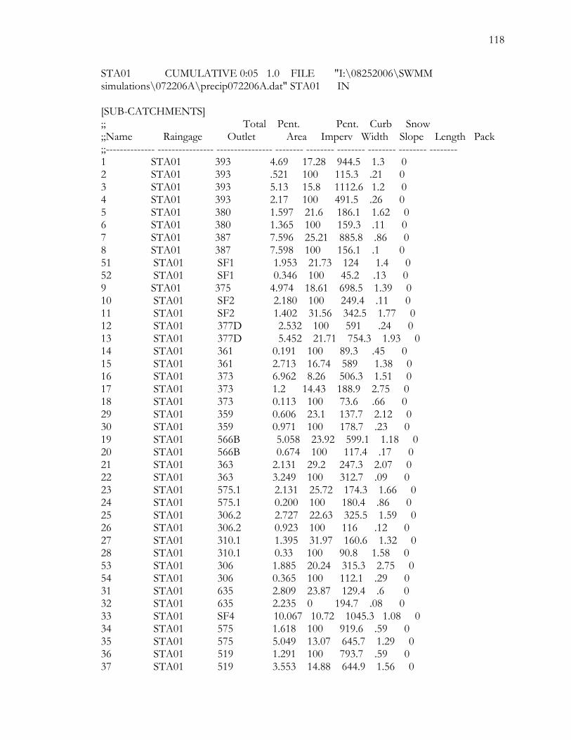
118

STA01 CUMULATIVE 0:05 1.0 FILE "I:\08252006\SWMM simulations\072206A\precip072206A.dat" STA01 IN [SUB-CATCHMENTS] ;; Total Pcnt. Pcnt. Curb Snow ;;Name Raingage Outlet Area Imperv Width Slope Length Pack ;;-------------- ---------------- ---------------- -------- -------- -------- -------- -------- -------- 1 STA01 393 4.69 17.28 944.5 1.3 0 2 STA01 393 .521 100 115.3 .21 0 3 STA01 393 5.13 15.8 1112.6 1.2 0 4 STA01 393 2.17 100 491.5 .26 0 5 STA01 380 1.597 21.6 186.1 1.62 0 6 STA01 380 1.365 100 159.3 .11 0 7 STA01 387 7.596 25.21 885.8 .86 0 8 STA01 387 7.598 100 156.1 .1 0 51 STA01 SF1 1.953 21.73 124 1.4 0 52 STA01 SF1 0.346 100 45.2 .13 0 9 STA01 375 4.974 18.61 698.5 1.39 0 10 STA01 SF2 2.180 100 249.4 .11 0 11 STA01 SF2 1.402 31.56 342.5 1.77 0 12 STA01 377D 2.532 100 591 .24 0 13 STA01 377D 5.452 21.71 754.3 1.93 0 14 STA01 361 0.191 100 89.3 .45 0 15 STA01 361 2.713 16.74 589 1.38 0 16 STA01 373 6.962 8.26 506.3 1.51 0 17 STA01 373 1.2 14.43 188.9 2.75 0 18 STA01 373 0.113 100 73.6 .66 0 29 STA01 359 0.606 23.1 137.7 2.12 0 30 STA01 359 0.971 100 178.7 .23 0 19 STA01 566B 5.058 23.92 599.1 1.18 0 20 STA01 566B 0.674 100 117.4 .17 0 21 STA01 363 2.131 29.2 247.3 2.07 0 22 STA01 363 3.249 100 312.7 .09 0 23 STA01 575.1 2.131 25.72 174.3 1.66 0 24 STA01 575.1 0.200 100 180.4 .86 0 25 STA01 306.2 2.727 22.63 325.5 1.59 0 26 STA01 306.2 0.923 100 116 .12 0 27 STA01 310.1 1.395 31.97 160.6 1.32 0 28 STA01 310.1 0.33 100 90.8 1.58 0 53 STA01 306 1.885 20.24 315.3 2.75 0 54 STA01 306 0.365 100 112.1 .29 0 31 STA01 635 2.809 23.87 129.4 .6 0 32 STA01 635 2.235 0 194.7 .08 0 33 STA01 SF4 10.067 10.72 1045.3 1.08 0 34 STA01 575 1.618 100 919.6 .59 0 35 STA01 575 5.049 13.07 645.7 1.29 0 36 STA01 519 1.291 100 793.7 .59 0 37 STA01 519 3.553 14.88 644.9 1.56 0

119

38 STA01 471 3.17 12.48 442.4 1.85 0 39 STA01 481 1.532 13.46 311.2 4.85 0 40 STA01 481 0.22 100 191.4 1.27 0 41 STA01 301.1 2.266 0 133 2.16 0 42 STA01 301.1 0.358 100 359.7 .96 0 43 STA01 468.1 4.623 0 425.1 .4 0 44 STA01 468.3 1.968 18.13 278 4.12 0 45 STA01 468.4 2.979 19.69 294.9 2.21 0 46 STA01 468.4 0.506 100 139.1 .26 0 48 STA01 SF3 6.28 14.95 948.7 3.45 0 49 STA01 SF3 0.906 100 295.8 .31 0 50 STA01 302 1.377 18.05 207.5 1.51 0 [SUBAREAS] ;;Sub-catchment N-Imperv N-Perv S-Imperv S-Perv PctZero RouteTo PctRouted ;;-------------- ---------- ---------- ---------- ---------- ---------- ---------- ---------- 1 0.012 0.15 .15 .2 25 OUTLET 2 0.012 0.15 .15 .2 25 OUTLET 3 0.012 0.15 .15 .2 25 OUTLET 4 0.012 0.15 .15 .2 25 OUTLET 5 0.012 0.15 .15 .2 25 OUTLET 6 0.012 0.15 .15 .2 25 OUTLET 7 0.012 0.15 .15 .2 25 OUTLET 8 0.012 0.15 .15 .2 25 OUTLET 51 0.012 0.15 .15 .2 25 OUTLET 52 0.012 0.15 .15 .2 25 OUTLET 9 0.012 0.15 .15 .2 25 OUTLET 10 0.012 0.15 .15 .2 25 OUTLET 11 0.012 0.15 .15 .2 25 OUTLET 12 0.012 0.15 .15 .2 25 OUTLET 13 0.012 0.15 .15 .2 25 OUTLET 14 0.012 0.15 .15 .2 25 OUTLET 15 0.012 0.15 .15 .2 25 OUTLET 16 0.012 0.15 .15 .2 25 OUTLET 17 0.012 0.15 .15 .2 25 OUTLET 18 0.012 0.15 .15 .2 25 OUTLET 29 0.012 0.15 .15 .2 25 OUTLET 30 0.012 0.15 .15 .2 25 OUTLET 19 0.012 0.15 .15 .2 25 OUTLET 20 0.012 0.15 .15 .2 25 OUTLET 21 0.012 0.15 .15 .2 25 OUTLET 22 0.012 0.15 .15 .2 25 OUTLET 23 0.012 0.15 .15 .2 25 OUTLET 24 0.012 0.15 .15 .2 25 OUTLET 25 0.012 0.15 .15 .2 25 OUTLET 26 0.012 0.15 .15 .2 25 OUTLET 27 0.012 0.15 .15 .2 25 OUTLET

120

28 0.012 0.15 .15 .2 25 OUTLET 53 0.012 0.15 .15 .2 25 OUTLET 54 0.012 0.15 .15 .2 25 OUTLET 31 0.012 0.15 .15 .2 25 OUTLET 32 0.012 0.15 .15 .2 25 OUTLET 33 0.012 0.15 .15 .2 25 OUTLET 34 0.012 0.15 .15 .2 25 OUTLET 35 0.012 0.15 .15 .2 25 OUTLET 36 0.012 0.15 .15 .2 25 OUTLET 37 0.012 0.15 .15 .2 25 OUTLET 38 0.012 0.15 .15 .2 25 OUTLET 39 0.012 0.15 .15 .2 25 OUTLET 40 0.012 0.15 .15 .2 25 OUTLET 41 0.012 0.15 .15 .2 25 OUTLET 42 0.012 0.15 .15 .2 25 OUTLET 43 0.012 0.15 .15 .2 25 OUTLET 44 0.012 0.15 .15 .2 25 OUTLET 45 0.012 0.15 .15 .2 25 OUTLET 46 0.012 0.15 .15 .2 25 OUTLET 48 0.012 0.15 .15 .2 25 OUTLET 49 0.012 0.15 .15 .2 25 OUTLET 50 0.012 0.15 .15 .2 25 OUTLET [INFILTRATION] ;;Sub-catchment CurveNum HydCon DryTime ;;-------------- ---------- ---------- ---------- 1 82.66 0.6 4 2 98 0.6 4 3 81.67 0.6 4 4 98 0.6 4 5 85.58 0.6 4 6 98 0.6 4 7 88 0.6 4 8 98 0.6 4 51 85.58 0.6 4 52 98 0.6 4 9 83.56 0.6 4 10 98 0.6 4 11 92.3 0.6 4 12 98 0.6 4 13 85.66 0.6 4 14 98 0.6 4 15 82.3 0.6 4 16 76.58 0.6 4 17 80.74 0.6 4 18 98 0.6 4 29 86.59 0.6 4 30 98 0.6 4

121

19 87.15 0.6 4 20 98 0.6 4 21 90.71 0.6 4 22 98 0.6 4 23 88.36 0.6 4 24 98 0.6 4 25 86.27 0.6 4 26 98 0.6 4 27 92.58 0.6 4 28 98 0.6 4 53 84.66 0.6 4 54 98 0.6 4 31 87.11 0.6 4 32 71 0.6 4 33 78.23 0.6 4 34 98 0.6 4 35 79.82 0.6 4 36 96.71 0.6 4 37 81.04 0.6 4 38 79.41 0.6 4 39 80.08 0.6 4 40 98 0.6 4 41 71 0.6 4 42 98 0.6 4 43 71 0.6 4 44 83.24 0.6 4 45 84.29 0.6 4 46 98 0.6 4 48 81.09 0.6 4 49 98 0.6 4 50 83.13 0.6 4 [JUNCTIONS] ;; Invert Max. Init. Surcharge Ponded ;;Name Elev. Depth Depth Depth Area ;;-------------- ---------- ---------- ---------- ---------- ---------- 393 1160.56 30.69 0 0 0 392 1159.64 31.37 0 0 0 387 1160.42 7.81 0 0 0 386 1157.66 19.23 0 0 0 380 1156.77 25.65 0 0 0 377 1153.92 17.88 0 0 0 377D 1170.63 13.58 0 0 0 645 1165.15 6.14 0 0 0 376 1152.12 11.31 0 0 0 375 1145.97 10.52 0 0 0 373 1133.79 9.23 0 0 0 361 1132.3 5.96 0 0 0

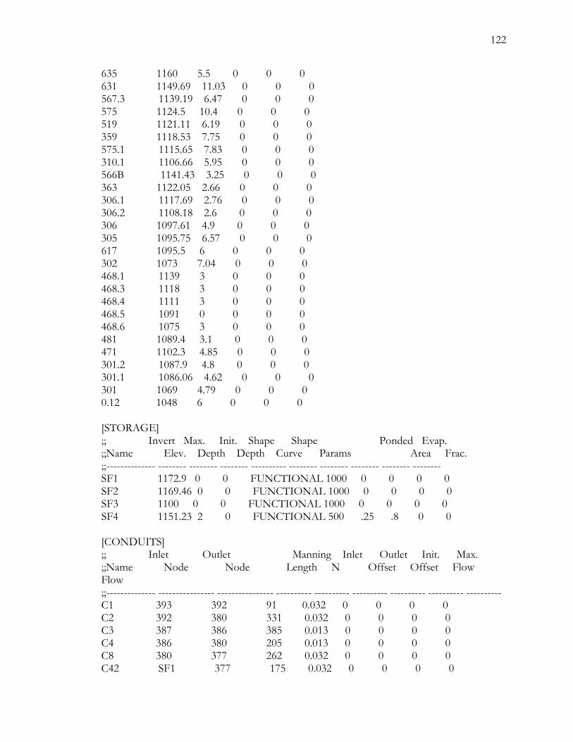
122

635 1160 5.5 0 0 0 631 1149.69 11.03 0 0 0 567.3 1139.19 6.47 0 0 0 575 1124.5 10.4 0 0 0 519 1121.11 6.19 0 0 0 359 1118.53 7.75 0 0 0 575.1 1115.65 7.83 0 0 0 310.1 1106.66 5.95 0 0 0 566B 1141.43 3.25 0 0 0 363 1122.05 2.66 0 0 0 306.1 1117.69 2.76 0 0 0 306.2 1108.18 2.6 0 0 0 306 1097.61 4.9 0 0 0 305 1095.75 6.57 0 0 0 617 1095.5 6 0 0 0 302 1073 7.04 0 0 0 468.1 1139 3 0 0 0 468.3 1118 3 0 0 0 468.4 1111 3 0 0 0 468.5 1091 0 0 0 0 468.6 1075 3 0 0 0 481 1089.4 3.1 0 0 0 471 1102.3 4.85 0 0 0 301.2 1087.9 4.8 0 0 0 301.1 1086.06 4.62 0 0 0 301 1069 4.79 0 0 0 0.12 1048 6 0 0 0 [STORAGE] ;; Invert Max. Init. Shape Shape Ponded Evap. ;;Name Elev. Depth Depth Curve Params Area Frac. ;;-------------- -------- -------- -------- ---------- -------- -------- -------- -------- -------- SF1 1172.9 0 0 FUNCTIONAL 1000 0 0 0 0 SF2 1169.46 0 0 FUNCTIONAL 1000 0 0 0 0 SF3 1100 0 0 FUNCTIONAL 1000 0 0 0 0 SF4 1151.23 2 0 FUNCTIONAL 500 .25 .8 0 0 [CONDUITS] ;; Inlet Outlet Manning Inlet Outlet Init. Max. ;;Name Node Node Length N Offset Offset Flow Flow ;;-------------- ---------------- ---------------- ---------- ---------- ---------- ---------- ---------- ---------- C1 393 392 91 0.032 0 0 0 0 C2 392 380 331 0.032 0 0 0 0 C3 387 386 385 0.013 0 0 0 0 C4 386 380 205 0.013 0 0 0 0 C8 380 377 262 0.032 0 0 0 0 C42 SF1 377 175 0.032 0 0 0 0

123

C9 377 376 149 0.032 0 0 0 0 C12 377D 645 263 0.032 0 0 0 0 C43 SF2 645 29 0.032 0 0 0 0 C10 645 376 376 0.032 0 0 0 0 C11 376 375 162 0.032 0 0 0 0 C6 375 373 267 0.032 0 0 0 0 C13 373 361 146 0.032 0 0 0 0 C15 361 359 347 0.032 0 0 0 0 C24 635 SF4 552 0.032 0 0 0 0 C25 SF4 631 45 0.032 0 0 0 0 C26 631 567.3 355 0.032 0 0 0 0 C27 567.3 519 819 0.032 0 0 0 0 C28 575 519 214 0.032 0 0 0 0 C29 519 359 112 0.032 0 0 0 0 C16 359 575.1 81 0.032 0 0 0 0 C19 575.1 310.1 277 0.032 0 0 0 0 C23 310.1 305 284 0.032 0 0 0 0 C17 566B 363 585 0.032 0 0 0 0 C18 363 306.1 225 0.032 0 0 0 0 C20 306.1 306.2 278 0.032 0 0 0 0 C21 306.2 306 241 0.032 0 0 0 0 C22 306 305 34 0.032 0 0 0 0 C38 305 302 446 0.032 0 0 0 0 C37 617 302 239 0.032 0 0 0 0 C39 302 301 101 0.032 0 0 0 0 C33 468.1 468.3 147 0.032 0 0 0 0 C34 468.3 468.4 178 0.032 0 0 0 0 C35 468.4 468.5 451 0.032 0 0 0 0 C41 468.5 468.6 253 0.05 0 0 0 0 C36 468.6 301 38 0.032 0 0 0 0 C31 481 301.2 117 0.032 0 0 0 0 C30 471 301.2 306 0.032 0 0 0 0 C32 301.2 301.1 109 0.013 0 0 0 0 C40 301.1 301 317 0.013 0 0 0 0 C0.12 301 0.12 324 0.032 0 0 0 0 C44 SF3 617 400 0.032 0 0 0 0 [XSECTIONS] ;;Link Shape Geom1 Geom2 Geom3 Geom4 Barrels ;;-------------- ------------ ---------------- ---------- ---------- ---------- ---------- C1 CIRCULAR 2 0 0 0 1 C2 CIRCULAR 3 0 0 0 1 C3 CIRCULAR 2 0 0 0 1 C4 CIRCULAR 2.5 0 0 0 1 C8 CIRCULAR 3 0 0 0 1 C42 CIRCULAR 1.25 0 0 0 1 C9 CIRCULAR 3 0 0 0 1 C12 CIRCULAR 2.5 0 0 0 1

124

C43 CIRCULAR 2.5 0 0 0 1 C10 CIRCULAR 2.5 0 0 0 1 C11 CIRCULAR 3 0 0 0 1 C6 CIRCULAR 3 0 0 0 1 C13 CIRCULAR 3 0 0 0 1 C15 CIRCULAR 3 0 0 0 1 C24 CIRCULAR 2.5 0 0 0 1 C25 CIRCULAR 1 0 0 0 1 C26 CIRCULAR 1.75 0 0 0 1 C27 CIRCULAR 2 0 0 0 1 C28 CIRCULAR 2 0 0 0 1 C29 CIRCULAR 2 0 0 0 1 C16 CIRCULAR 3 0 0 0 1 C19 CIRCULAR 3 0 0 0 1 C23 CIRCULAR 3 0 0 0 1 C17 CIRCULAR 1.5 0 0 0 1 C18 CIRCULAR 1.5 0 0 0 1 C20 CIRCULAR 1.5 0 0 0 1 C21 CIRCULAR 2.5 0 0 0 1 C22 CIRCULAR 3 0 0 0 1 C38 CIRCULAR 3 0 0 0 1 C37 CIRCULAR 1.25 0 0 0 1 C39 CIRCULAR 3 0 0 0 1 C33 CIRCULAR 1 0 0 0 1 C34 CIRCULAR 1.5 0 0 0 1 C35 CIRCULAR 1.5 0 0 0 1 C41 TRAPEZOIDAL 1.5 1 .5 0.5 1 C36 CIRCULAR 1.5 0 0 0 1 C31 CIRCULAR 1.25 0 0 0 1 C30 CIRCULAR 1.5 0 0 0 1 C32 CIRCULAR 2 0 0 0 1 C40 CIRCULAR 2 0 0 0 1 C0.12 CIRCULAR 4 0 0 0 1 C44 CIRCULAR 1 0 0 0 1 [LOSSES] ;;Link Inlet Outlet Average Flap Gate ;;-------------- ---------- ---------- ---------- ---------- [TIMESERIES] ;;Name Date Time Value ;;-------------- ---------- ---------- ---------- ;7/22/2006 7:05 68.4 072206 7/22/2006 7:10 68.6 072206 7/22/2006 7:15 68.7 072206 7/22/2006 7:20 68.7 072206 7/22/2006 7:25 68.7 072206 7/22/2006 7:30 68.8

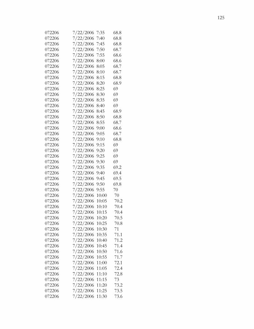
125

072206 7/22/2006 7:35 68.8 072206 7/22/2006 7:40 68.8 072206 7/22/2006 7:45 68.8 072206 7/22/2006 7:50 68.7 072206 7/22/2006 7:55 68.6 072206 7/22/2006 8:00 68.6 072206 7/22/2006 8:05 68.7 072206 7/22/2006 8:10 68.7 072206 7/22/2006 8:15 68.8 072206 7/22/2006 8:20 68.9 072206 7/22/2006 8:25 69 072206 7/22/2006 8:30 69 072206 7/22/2006 8:35 69 072206 7/22/2006 8:40 69 072206 7/22/2006 8:45 68.9 072206 7/22/2006 8:50 68.8 072206 7/22/2006 8:55 68.7 072206 7/22/2006 9:00 68.6 072206 7/22/2006 9:05 68.7 072206 7/22/2006 9:10 68.8 072206 7/22/2006 9:15 69 072206 7/22/2006 9:20 69 072206 7/22/2006 9:25 69 072206 7/22/2006 9:30 69 072206 7/22/2006 9:35 69.2 072206 7/22/2006 9:40 69.4 072206 7/22/2006 9:45 69.5 072206 7/22/2006 9:50 69.8 072206 7/22/2006 9:55 70 072206 7/22/2006 10:00 70 072206 7/22/2006 10:05 70.2 072206 7/22/2006 10:10 70.4 072206 7/22/2006 10:15 70.4 072206 7/22/2006 10:20 70.5 072206 7/22/2006 10:25 70.8 072206 7/22/2006 10:30 71 072206 7/22/2006 10:35 71.1 072206 7/22/2006 10:40 71.2 072206 7/22/2006 10:45 71.4 072206 7/22/2006 10:50 71.6 072206 7/22/2006 10:55 71.7 072206 7/22/2006 11:00 72.1 072206 7/22/2006 11:05 72.4 072206 7/22/2006 11:10 72.8 072206 7/22/2006 11:15 73 072206 7/22/2006 11:20 73.2 072206 7/22/2006 11:25 73.5 072206 7/22/2006 11:30 73.6

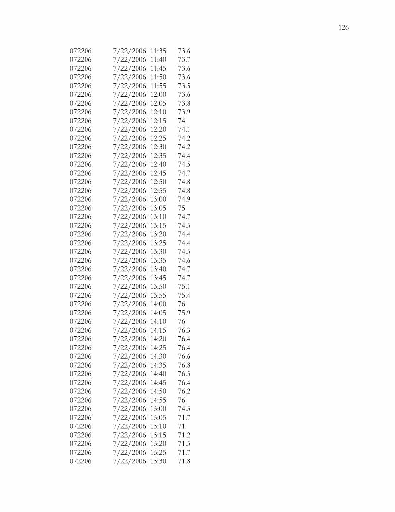
126

072206 7/22/2006 11:35 73.6 072206 7/22/2006 11:40 73.7 072206 7/22/2006 11:45 73.6 072206 7/22/2006 11:50 73.6 072206 7/22/2006 11:55 73.5 072206 7/22/2006 12:00 73.6 072206 7/22/2006 12:05 73.8 072206 7/22/2006 12:10 73.9 072206 7/22/2006 12:15 74 072206 7/22/2006 12:20 74.1 072206 7/22/2006 12:25 74.2 072206 7/22/2006 12:30 74.2 072206 7/22/2006 12:35 74.4 072206 7/22/2006 12:40 74.5 072206 7/22/2006 12:45 74.7 072206 7/22/2006 12:50 74.8 072206 7/22/2006 12:55 74.8 072206 7/22/2006 13:00 74.9 072206 7/22/2006 13:05 75 072206 7/22/2006 13:10 74.7 072206 7/22/2006 13:15 74.5 072206 7/22/2006 13:20 74.4 072206 7/22/2006 13:25 74.4 072206 7/22/2006 13:30 74.5 072206 7/22/2006 13:35 74.6 072206 7/22/2006 13:40 74.7 072206 7/22/2006 13:45 74.7 072206 7/22/2006 13:50 75.1 072206 7/22/2006 13:55 75.4 072206 7/22/2006 14:00 76 072206 7/22/2006 14:05 75.9 072206 7/22/2006 14:10 76 072206 7/22/2006 14:15 76.3 072206 7/22/2006 14:20 76.4 072206 7/22/2006 14:25 76.4 072206 7/22/2006 14:30 76.6 072206 7/22/2006 14:35 76.8 072206 7/22/2006 14:40 76.5 072206 7/22/2006 14:45 76.4 072206 7/22/2006 14:50 76.2 072206 7/22/2006 14:55 76 072206 7/22/2006 15:00 74.3 072206 7/22/2006 15:05 71.7 072206 7/22/2006 15:10 71 072206 7/22/2006 15:15 71.2 072206 7/22/2006 15:20 71.5 072206 7/22/2006 15:25 71.7 072206 7/22/2006 15:30 71.8

127

072206 7/22/2006 15:35 71.7 072206 7/22/2006 15:40 71.6 072206 7/22/2006 15:45 71.3 072206 7/22/2006 15:50 71 072206 7/22/2006 15:55 70.7 072206 7/22/2006 16:00 70.4 072206 7/22/2006 16:05 70.2 072206 7/22/2006 16:10 70.1 072206 7/22/2006 16:15 70.2 072206 7/22/2006 16:20 70.3 072206 7/22/2006 16:25 70.2 072206 7/22/2006 16:30 70.2 072206 7/22/2006 16:35 70 072206 7/22/2006 16:40 69.8 072206 7/22/2006 16:45 69.9 072206 7/22/2006 16:50 69.8 072206 7/22/2006 16:55 69.6 072206 7/22/2006 17:00 69.9 [REPORT] INPUT NO CONTROLS NO

128

Appendix B.2: ECDA-SWMM catchment, node, and link representation of the ECDA

129

Appendix B.3: All 29 Storm events observed, uncalibrated and calibrated peak runoff and total volume data (the 5 storms used in the ECDA-SWMM scenarios are in bold)

Storm Event

P (in.)

Obs. Qp (CFS)

Obs. VT (acre-ft)

Uncal. Qp (CFS)

Uncal. VT (acre-ft)

Cal. Qp (CFS)

Cal. VT (acre-ft)

1 06/27/06 1.52 31.2 4.38 56.7 7.60 33.1 4.69

2 07/11/07 1.20 34.0 1.44 72.0 3.94 64.6 3.07

3 06/03/07 1.12 24.4 1.82 61.7 5.03 44.7 3.07

4 06/03/06 0.960 11.6 2.09 31.8 4.62 17.9 2.72

5 06/04/06 0.960 11.8 1.59 52.4 3.11 32.9 1.20

6 06/22/06 0.500 40.7 1.27 68.6 2.37 36.7 1.26

7 06/23/06 0.480 12.0 1.50 21.6 1.98 8.86 1.00

8 07/12/06 0.440 7.06 0.918 37.6 1.28 14.9 0.574

9 07/15/06 0.440 18.8 0.624 56.7 1.85 8.55 0.286

10 06/26/06 0.420 9.75 1.64 21.0 1.56 8.17 0.757

11 7/22/06 (1) 0.380 16.8 0.730 39.0 1.51 18.8 0.738

12 07/05/07 0.380 7.69 0.274 56.8 1.64 28.1 0.808

13 07/02/06 0.350 12.2 0.374 52.9 1.44 24.1 0.738

14 06/08/07 0.320 5.41 0.210 20.0 0.639 5.17 0.219

15 05/10/07 0.320 5.60 0.126 19.7 1.23 9.15 0.567

16 6/23/06 (1) 0.280 12.0 0.755 21.6 1.03 5.10 0.456

17 05/31/06 0.260 7.68 0.132 30.7 0.972 8.91 0.413

18 7/12/06 (2) 0.260 7.06 0.460 16.1 0.958 6.41 0.404

19 6/19/07 (2) 0.260 8.24 0.484 47.2 1.20 14.1 0.563

20 6/19/07 (1) 0.230 8.22 0.232 43.8 0.902 10.1 0.339

21 05/31/07 0.230 4.56 0.476 10.7 0.709 3.58 0.281

22 05/26/06 0.220 6.06 0.519 8.98 0.695 3.19 0.278

23 05/16/07 0.210 12.0 0.755 12.0 0.627 2.00 0.220

24 06/12/07 0.200 7.40 0.189 31.1 0.758 9.35 0.296

25 7/11/07 (2) 0.200 15.3 0.469 27.8 0.573 6.57 0.200

26 07/27/06 0.190 10.3 0.335 24.5 0.838 4.79 0.206

27 06/01/06 0.190 8.07 0.200 25.0 0.584 6.43 0.222

28 06/25/06 0.190 2.77 0.580 3.26 0.432 0.888 0.137

29 7/22/06 (2) 0.140 15.4 0.371 8.55 0.286 2.12 0.0943

130

Appendix B.4: All 29 Storm events uncalibrated, and calibrated peak runoff and total volume data normalized with the observed runoff (simulated/observed) (The 5 storms used in the ECDA-SWMM scenarios are in bold)

Storm Event P (in.) Norm. Uncal.

Qp

Norm. Uncal. VT

Norm. Cal. Qp

Norm. Cal. VT

1 06/27/06 1.52 1.82 1.74 1.06 1.07

2 07/11/07 1.20 2.12 2.74 1.90 2.14

3 06/03/07 1.12 2.53 2.76 1.83 1.68

4 06/03/06 0.960 2.734 2.21 1.54 1.30

5 06/04/06 0.960 4.43 1.97 2.78 0.756

6 06/22/06 0.500 1.69 1.86 0.900 0.991

7 06/23/06 0.480 1.80 1.32 0.740 0.670

8 07/12/06 0.440 5.33 1.40 2.11 0.625

9 07/15/06 0.440 3.01 2.97 0.454 0.458

10 06/26/06 0.420 2.15 0.956 0.838 0.463

11 7/22/06 (1) 0.380 2.32 2.06 1.12 1.01

12 07/05/07 0.380 7.38 5.98 3.66 2.95

13 07/02/06 0.350 4.34 3.84 1.98 1.97

14 06/08/07 0.320 3.69 3.04 0.956 1.04

15 05/10/07 0.320 3.51 9.78 1.63 4.50

16 6/23/06 (1) 0.280 1.80 1.37 0.426 0.604

17 05/31/06 0.260 3.99 7.36 1.160 3.13

18 7/12/06 (2) 0.260 2.28 2.08 0.908 0.878

19 6/19/07 (2) 0.260 5.74 2.47 1.71 1.16

20 6/19/07 (1) 0.230 5.33 3.89 1.23 1.46

21 05/31/07 0.230 2.35 1.49 0.785 0.590

22 05/26/06 0.220 1.48 1.34 0.527 0.536

23 05/16/07 0.210 1.00 0.830 0.167 0.291

24 06/12/07 0.200 4.20 4.01 1.26 1.57

25 7/11/07 (2) 0.200 1.81 1.22 0.429 0.426

26 07/27/06 0.190 2.38 2.50 0.466 0.615

27 06/01/06 0.190 3.10 2.92 0.797 1.11

28 06/25/06 0.190 1.18 0.745 0.320 0.236

29 7/22/06 (2) 0.140 0.555 0.771 0.138 0.254

Average Normalized % 2.97 2.68 1.17 1.19

131

Appendix B.5: Mean normalized percentage error (MNPE) for the uncalibrated and calibrated simulations of all 29 storm events

Storm Event P

(in.) Uncal. Qp

NPE Uncal. VT

NPE Calib. Qp

NPE Calib. VT

NPE

1 6/27/2006 1.52 81.7% 73.6% 5.90% 7.05%

2 7/11/2007 1.20 112% 174% 90.1% 114%

3 6/3/2007 1.12 153% 176% 83.5% 68.2%

4 6/3/2006 0.96 173% 121% 53.8% 30.0%

5 6/4/2006 0.96 343% 96.4% 178% -24.4%

6 6/22/2006 0.50 68.6% 86.3% -0.940% -9.96%

7 6/23/2006 0.48 80.5% 32.2% 26.0% -33.0%

8 7/12/2006 0.44 432% 39.7% 110% -37.5%

9 7/15/2006 0.44 201% 197% -54.6% -54.2%

10 6/26/2006 0.42 115% -4.40% 16.2% -53.7%

11 7/5/2007 0.38 638% 498% 265% 194.9%

12 7/22/2006(1) 0.38 132% 107% 11.9% 1.10%

13 7/2/2006 0.35 334% 284% 98.2% 97.3%

14 5/10/2007 0.32 251% 878% 63.4% 350%

15 6/8/2007 0.32 269% 204% -4.40% 4.29%

16 6/23/06(1) 0.28 80.5% 36.7% -57.4% -39.6%

17 5/31/2006 0.26 300% 636% 16.0% 213%

18 6/19/2007(2) 0.26 473.4% 147% 70.9% 16.3%

19 7/12/2006(2) 0.26 128% 108% -9.22% -12.2%

20 5/31/2007 0.23 135% 49.0% -21.5% -41.0%

21 6/19/2007(1) 0.23 433% 288% 23.0% 46.1%

22 5/26/2006 0.22 48.1% 33.8% -47.3% -46.4%

23 5/16/2007 0.21 0.030% -17.0% -83.3% -70.9%

24 6/12/2007 0.20 320% 301% 26.4% 56.6%

25 7/11/2007(2) 0.20 81.1% 22.2% -57.4% -57.4%

26 7/27/2006 0.19 138% 150% -53.4% -38.5%

27 6/25/2006 0.19 17.8% -25.5% -68.0% -76.4%

28 6/1/2006 0.19 210% 192.% -24.13% 11.0%

29 7/22/2006(2) 0.14 -44.5% -22.9% -86.23% -74.6%

MNPEX 196% 168% 19.72% 18.6%

132

Appendix B.6: Normalized observed total volume data and uncalibrated total volume data with the maximum amount of rainfall for the ECDA

Storm Event

P. (in.)

Obs. VT (acre-ft)

Uncal. VT (acre-ft)

Max VT (acre-ft)

Obs. VT /Max VT

Uncal. VT /Max VT

1 6/27/2006 1.52 4.38 7.60 24.3 0.180 0.313

2 7/11/2007 1.20 1.44 3.94 19.2 0.075 0.205

3 6/3/2007 1.12 1.82 5.03 17.9 0.102 0.281

4 6/3/2006 0.960 2.09 4.62 15.4 0.136 0.301

5 6/4/2006 0.960 1.59 3.11 15.4 0.103 0.203

6 6/22/2006 0.500 1.27 2.37 8.00 0.159 0.297

7 6/23/2006 0.480 1.50 1.98 7.68 0.195 0.258

8 7/12/2006 0.440 0.918 1.28 7.04 0.130 0.182

9 7/15/2006 0.440 0.624 1.85 7.04 0.089 0.263

10 6/26/2006 0.420 1.64 1.56 6.72 0.244 0.233

11 7/22/06 (1) 0.380 0.730 1.51 6.08 0.120 0.248

12 7/5/2007 0.380 0.274 1.64 6.08 0.045 0.270

13 7/2/2006 0.350 0.374 1.44 5.60 0.067 0.257

14 6/8/2007 0.320 0.210 0.639 5.12 0.041 0.125

15 5/10/2007 0.320 0.126 1.23 5.12 0.025 0.241

16 6/23/06 (1) 0.280 0.755 1.03 4.48 0.169 0.230

17 5/31/2006 0.260 0.132 0.972 4.16 0.032 0.234

18 7/12/06 (2) 0.260 0.460 0.958 4.16 0.111 0.230

19 6/19/07 (2) 0.260 0.484 1.20 4.16 0.116 0.288

20 6/19/07A (1) 0.230 0.232 0.902 3.68 0.063 0.245

21 5/31/2007 0.230 0.476 0.709 3.68 0.129 0.193

22 5/26/2006 0.220 0.519 0.695 3.52 0.148 0.198

23 5/10/2007 0.210 0.126 1.23 3.36 0.038 0.367

24 5/16/2007 0.210 0.755 0.627 3.36 0.225 0.187

25 6/12/2007 0.200 0.189 0.758 3.20 0.059 0.237

26 7/11/07 (2) 0.200 0.469 0.573 3.20 0.147 0.179

27 7/27/2006 0.190 0.335 0.838 3.04 0.110 0.276

28 6/1/2006 0.190 0.200 0.584 3.04 0.066 0.192

29 6/25/2006 0.190 0.580 0.432 3.04 0.191 0.142

30 7/22/06 (2) 0.140 0.371 0.286 2.24 0.166 0.128

Ko = 0.116

Ks = 0.233

133

APPENDIX C

Propositional Paper for the State College Borough

134

State College Borough Rainwater Harvesting Project

Brief

The State College Borough Rainwater Harvesting proposal is the development of a system

that provides incentives for residential and commercial buildings to manage their stormwater

on-site in a decentralized manner that reduces contribution to the borough stormwater

network, manifesting multiple sustainable and positive benefits in terms of reduction of

flooding events, decreasing constituents of stormwater pollution, increasing water

conservation, and the treatment of rainwater as a precious resource

Background and Discussion

The State College Borough has, as a matter of good environmental policy and as part of the

climate protection declaration (Resolution 944) determined to set “specific goals including to

establish incentives for the installation of green roofs, rainwater cisterns, and other best

management practices to reduce urban runoff” by 2012.

The stormwater problems facing the State College Borough include infrastructure damage

from flooding, high stormwater quantity stream degradation, and potential water quality

pollution (Lebzelter, 1998; Smeltz, 2005). The Spring Creek Watershed currently has over

16.2 miles of impaired streams as a result of increased sediment loading and increased

temperatures (CC, 2007). The Centre County Planning Commission identified 48 areas in the

region that are flood prone (Hopkins, 2002). The Millbrook Marsh wetland's viability is

135

being threatened from stormwater input (Lipton, 1998). To make matters worse, climate

change is forecasted to increase the amount of floodwater in the region with higher intensity

rainfall exacerbating the State College Borough stormwater problem.

Technically, stormwater is a source of possible pollution and arguably a waste, and could

have the same principles applied to as it as wastewater management, which attracts a disposal

fee via either specific charges or through property taxes.

Environmental benefits of this proposal include:

Reduced volume and peak flow rates to discharging water which causes erosion,

constituents of pollution, turbidity and flooding.

Reduction of erosion of water ways and consequently a reduction of maintenance

requirements.

Improved water quality through capture of first flush contaminated water.

Reduced impact on the habitat of receiving waters through the improvement of

quality of runoff.

Increased reuse of rainwater in a decentralized manner, reducing pressure on water

mains and decreasing the cost of pumping groundwater.

Improve the health amenity and vitality of landscaping and vegetation, particularly

during times of water restrictions.

Additional social and Borough benefits

Restore natural groundwater by infiltrating additional stormwater being processed by

the wastewater treatment plant.

136

Improve security of groundwater.

Reduced impact of flooding damage during storm events.

Incentives and rewards to encourage all individuals to take action rather than only

those that are environmentally conscious.

Provide leadership to the greater State College community, including the

Susquehanna River Basin, on stormwater management action.

RECOMMENDATION

It is recommended to the Borough of State College that:

1. The Borough should provide workshops and literature related to simple and cost-

effective rainwater harvesting examples.

2. The Borough offer rebates of up $500 on the cost of installing a rainwater harvesting

system.

3. The Borough should endorse in principle the concept of a “charge and rebate

system” for stormwater runoff from residential and commercial properties to local

stormwater infrastructure