radiocarbon - geophysical fluid dynamics laboratory · pdf filea constant atmospheric...

Radiocarbon Measurements. Uranium+ThoriumDecay Series in the Oceans Overview.

Further ReadingGuary JC, Guegueniat P and Pentreath RJ (eds) (1988)

Radionuclides: A Tool for Oceanography. London,New York: Elsevier Applied Science.

Hunt GJ, Kershaw PJ and Swift DJ (eds) (1998)Radionuclides in the oceans (RADOC 96}97). Distri-

bution, Models and Impacts. Radiation ProtectionDosimetry 75 (1}4) 1998.

IAEA (1995) Environmental impact of radioactive re-leases; Proceedings of an International Symposium onEnvironmental Impact of Radioactive Releases. Inter-national Atomic Energy Agency, Vienna, 1995.

IAEA (1999) Inventory of Radioactive Waste Disposalsat Sea. IAEA-TECDOC-1105. International AtomicEnergy Agency, Vienna, August 1999, pp. 24A.1}A.22.

RADIOCARBON

R. M. Key, Princeton University, Princeton, NJ, USA

Copyright ^ 2001 Academic Press

doi:10.1006/rwos.2001.0162

Introduction

In 1934 F.N.D. Kurie at Yale University obtainedthe Rrst evidence for existence of radiocarbon(carbon-14, 14C). Over the next 20 years most ofthe details for measuring 14C and for its applicationto dating were worked out by W.F. Libby andco-workers. Libby received the 1960 Nobel Prize inchemistry for this research.

The primary application of 14C is to date objectsor to determine various environmental process rates.The 14C method is based on the assumption ofa constant atmospheric formation rate. Once pro-duced, atmospheric 14C reacts to form 14CO2, whichparticipates in the global carbon cycle processes ofphotosynthesis and respiration as well as the phys-ical processes of dissolution, particulate deposition,evaporation, precipitation, transport, etc. Atmo-spheric radiocarbon is transferred to the oceanprimarily by air}sea gas exchange of 14CO2. Once inthe ocean, 14CO2 is subject to the same physical,chemical, and biological processes that affect CO2.While alive, biota establish an equilibrium concen-tration of radiocarbon with their surroundings; thatis, 14C lost by decay is replaced by uptake from theenvironment. Once the tissue dies or is removedfrom an environment that contains 14C, the decay isno longer compensated. The loss of 14C by decaycan then be used to determine the time of death orremoval from the original 14C source. After death orremoval of the organism, it is generally assumedthat no exchange occurs between the tissue and itssurroundings; that is, the system is assumed to beclosed. As a result of the 14C decay rate, the various

reservoir sizes involved in the carbon cycle, andexchange rates between the reservoirs, the oceancontains approximately 50 times as much naturalradiocarbon as does the atmosphere.

Carbon-14 is one of three naturally occurringcarbon isotopes; 14C is radioactive, has a half-life of5730 years and decays by emitting a b-particle withan energy of about 156 keV. On the surface of theearth, the abundance of natural 14C relative to thetwo stable naturally occurring carbon isotopes is12C : 13C : 14C"98.9% : 1.1% : 1.2]10~10 %. Natu-ral radiocarbon is produced in the atmosphere,primarily by the collision of cosmic ray producedneutrons with nitrogen according to the reaction [I].

10n#14

7 NN146 C#

11H [I]

where n is a neutron and H is the proton emittedby the product nucleus. Similarly, the decay of14C takes place by emission of a b-particle and leadsto stable nitrogen according to reaction [II],

146 CN

147 N#b~#l6 #Q [II]

where l6 is an antineutrino and Q is the decayenergy.

The atmospheric production rate varies somewhatand is inSuenced by changes in the solar wind andin the earth’s geomagnetic Reld intensity. A mean of1.57 atom cm~2 s~1 is estimated based on the long-term record preserved in tree rings and a carbonreservoir model. This long-term production rateyields a global natural 14C inventory of approxim-ately 50 t (1 t"106 g). Production estimates basedon the more recent record of neutron Sux measure-ments tend to be higher, with values approaching2 atom cm~2 s~1. Figure 1 shows the atmospherichistory of 14C from AD 1511 to AD 1954 measuredby Minze Stuiver (University of Washington) usingtree growth rings. The strong decrease that occurs

2338 RADIOCARBON

VVCrSVKrNPrScanrKalairRWOS 057

−20

−10

0

10

20

1500 1600 1700 1800 1900

Year

∆14C

(pp

t)

Figure 1 Atmospheric history of *14C measured by M. Stuiverin tree rings covering AD 1511 to AD 1954. Most of the decreaseover the last hundred years is due to the addition of anthropo-genic CO2 to the atmosphere during the industrial revolution bythe burning of fossil fuels.

after about AD 1880 is due to dilution by anthropo-genic addition of CO2 during the industrial revol-ution by the burning of fossil fuels (coal, gas, oil).This dilution has come to be known as the Suesseffect (after Hans E. Suess).

Prior to 16 July 1945 all radiocarbon on thesurface of the earth was produced naturally. Onthat date, US scientists carried out the Rrst atmo-spheric atomic bomb test, known as the TrinityTest. Between 1945 and 1963, when the Partial TestBan Treaty was signed and atmospheric nucleartesting was banned, approximately 500 atmosphericnuclear explosions were carried out by the UnitedStates (215), the former Soviet Union (219), theUnited Kingdom (21) and France (50). After thesigning, a few additional atmospheric tests werecarried out by China (23) and other countries notparticipating in the treaty. The net effect of thetesting was to signiRcantly increase 14C levels in theatmosphere and subsequently in the ocean. Anthro-pogenic 14C has also been added to the environmentfrom some nuclear power plants, but this input isgenerally only detectable near the reactor.

It is unusual to think of any type of atmosphericcontamination d especially by a radioactive speciesd as beneRcial; however, bomb-produced radio-carbon (and tritium) has proven to be extremelyvaluable to oceanographers. The majority of theatmospheric testing, in terms of number of tests and14C production, occurred over a short time interval,between 1958 and 1963, relative to many oceancirculation processes. This time history, coupledwith the level of contamination and the fact that14C becomes intimately involved in the oceanic car-bon cycle, allows bomb-produced radiocarbon to be

valuable as a tracer for several ocean processesincluding biological activity, airdsea gas exchange,thermocline ventilation, upper ocean circulation,and upwelling.

Oceanographic radiocarbon results are generallyreported as *14C, the activity ratio relative to a stan-dard (NBS oxalic acid, 13.56 dpm per g of carbon)with a correction applied for dilution of theradiocarbon by anthropogenic CO2 with age correc-tions of the standard material to AD 1950. *14C isdeRned by eqn [1].

*14C"d14C!2(d13C#25)A1#d14C1000B [1]

d14C is given by eqn [2] and the deRnition of d13C isanalogous to that for d14C.

d14C"C14C/CDsmp!

14C/CDstd14C/CDstd D]1000 [2]

The Rrst part of the second term in the right sideof eqn [1] 2(d13C#25), corrects for fractionationeffects. The factor of 2 accounts for the fact that14C fractionation is expected to be twice as much asfor 13C and the additive constant 25 is a normaliz-ation factor conventionally applied to all samplesand based on the mean value of terrestrial wood.The details of 14C calculations can be signiRcantlymore involved than expressed in the above equa-tions; however, there is a general consensus that thecalculations and reporting of results be done asdescribed by Minze Stuiver and Henry Polach ina paper speciRcally written to eliminate differencesthat existed previously. *14C has units of parts perthousand (ppt). That is, 1 ppt means that 14C/12C forthe sample is greater than 14C/12C for the standardby 0.001. In these units the radioactive decay rate of14C is approximately 1 ppt per 8.1 years.

The number of surface ocean measurements madebefore any bomb-derived contamination are insufR-cient to provide the global distribution before inputfrom explosions. It is now possible to measure *14Cvalues in the annual growth rings of corals. Byestablishment of the exact year associated with eachring, reconstruction of the surface ocean *14C his-tory is possible. Applying the same procedure tolong-lived mollusk shells extends the method tohigher latitudes than is possible with corals.Whether corals or shells are used, it must be demon-strated that the coral or shell incorporates 14C in thesame ratio as the water in which it grew or at leastthat the fractionation is known. This method worksonly over the depth range at which the animal lived.

RADIOCARBON 2339


−50

0

50

100

1700 1800 1900 2000

Year

∆14C

(pp

t)

Figure 2 Long-term history of *14C in the surface PacificOcean measured by E. Druffel in two coral reefs. The verticallines surround the period of atmospheric nuclear weapons test-ing. The oceanic response to bomb contamination is delayedrelative to the atmosphere because of the relatively long equili-bration time between the ocean and atmosphere for 14CO2.

Year

1940 1950 1960 1970 1980 1990

0

200

600

1000 New ZealandGermanyTree Ring

• • •• • •• • •

Year

1940 1950 1960 1970 1980 1990

−100

0

50

150

DruffelToggweiler

North Pacific = FilledSouth Pacific = Empty

800∆14

C (

ppt)

400

−50

200

100

∆14C

(pp

t)

(A)

(B)

Figure 3 (A) Detailed atmospheric *14C history as recorded intree rings for times prior to 1955 and in atmospheric gas sam-ples from both New Zealand and Germany subsequently. Thelarge increase in the late 1950s and 1960s was due to theatmospheric testing of nuclear weapons (primarily fusion devi-ces). The hemispheric difference during the 1960s is becausemost atmospheric bomb tests were carried out north of theEquator and there is a resistance to atmospheric mixing acrossthe equator. Atmospheric levels began to decline shortly afterthe ban on atmospheric bomb testing. (B) *14C in the surfacePacific Ocean as recorded in the annual growth rings of corals.The same general trend seen in the atmosphere is present. Thebomb contamination peak is broadened and time-lagged relativeto the atmosphere due to both mixing and to the time requiredfor transfer from the atmosphere to the ocean.

Figure 2 shows the *14C record from two PaciRccoral reefs measured by Ellen Druffel. Vertical linesindicate the period of atmospheric nuclear tests(1945}1963). The relatively small variability overthe Rrst &300 years of the record includes vari-ations due to weather events, climate change, oceancirculation, atmospheric production, etc. The last 50years of the sequence records the invasion of bomb-produced *14C. Worth noting is the fact that thecoral record of the bomb signal is lagged. That is,the coral values did not start to increase immediate-ly testing began nor did they cease to increase whenatmospheric testing ended. The lag is due to thetime for the northern and southern hemisphereatmospheres to mix (&1 year) and to the relativelylong time required for the surface ocean toequilibrate with the atmosphere with respect to*14C (&10 years). Because of the slow equilibration,the surface ocean is frequently not at equilibriumwith the atmosphere. This disequilibrium is one ofthe reasons why pre-bomb surface ocean results,when expressed as ages rather than ppt units,are generally ‘old’ rather than ‘zero’ as might beexpected.

Figure 3A shows measured atmospheric *14Clevels from 1955 to the present in New Zealand(data from T.A. Rafter, M.A. Manning, and co-workers) and Germany (data from K.O. Munnichand co-workers) as well as older estimates based ontree ring measurements (data from M. Stuiver). Thebeginning of the signiRcant increase in the mid-1950s marks the atmospheric testing of hydrogenbombs. Atmospheric levels increased rapidly fromthat point until the mid-1960s. Soon after the banon atmospheric testing, levels began a decrease thatcontinues up to the present. The rate of decrease in

the atmosphere is about 0.055 y~1. Also clearly evi-dent in the Rgure is that the German measurementswere signiRcantly higher than those from New Zea-land between approximately 1962 and 1970. Thedifference reSects the facts that most of the atmo-spheric tests were carried out in the Northern Hemi-sphere and that approximately 1 year is required foratmospheric mixing across the Equator. During thatinterval some of the atmospheric 14CO2 is removed.Once atmospheric testing ceased, the two hemi-spheres equilibrated to the same radiocarbon level.

Figure 3B shows detailed PaciRc Ocean *14Ccoral ring data (J.R. Toggwelier and E. Druffel).This surface ocean record shows an increase duringthe 1960s; however, the peak occurs somewhat laterthan in the atmosphere and is signiRcantly less

2340 RADIOCARBON


pronounced. Careful investigation of coral data alsodemonstrates the north}south difference evidencedin the atmospheric record.

Sampling and MeasurementTechniques

The radiocarbon measurement technique has existedfor only 50 years. The Rrst 14C measurement wasmade in W.F. Libby’s Chicago laboratory in 1949and the Rrst list of ages was published in 1951.A necessary prerequisite to the age determinationwas accurate measurement of the radiocarbonhalf-life. This was done in 1949 in Antonia Engel-keimer’s laboratory at the Argonne National Labor-atory. Between 1952 and 1955 several additionalradiocarbon dating laboratories opened. By theearly 1960s several important advances had occur-red including the following.

f SigniRcantly improved counting efRciency andlower counting backgrounds, resulting in muchgreater measurement precision and longer time-scale over which the technique was applicable.

f Development of the extraction and concentrationtechnique for sea water samples.

f More precise determination of the half-life bythree different laboratories.

f Recognition by Hans Suess, while at the USGSand Scripps Institution of Oceanography, thatradiocarbon in modern samples (since the begin-ning of the industrial revolution) was beingdiluted by anthropogenic CO2 addition to theatmosphere and biosphere.

f Recognition that atmospheric and oceanic *14Clevels were increasing as a result of atmospherictesting of nuclear weapons.

During the 1970s and 1980s incremental changesin technique and equipment further increased theprecision and lowered the counting background.With respect to the ocean, this was a period ofsample collection, analysis, and interpretation. Thenext signiRcant change occurred during the 1990swith application of the accelerator mass spectro-metry (AMS) technique to oceanic samples. Thistechnique counts 14C atoms rather than detectingthe energy released when a 14C atom decays. TheAMS technique allowed reduction of the sample sizerequired for oceanic *14C determination from ap-proximately 250 liters of water to 250 milliliters! By1995 the AMS technique was yielding results thatwere as good as the best prior techniques using largesamples and decay counting. This size reduction and

concurrent automation procedures had a profoundeffect on sea water *14C determination. Many of theAMS techniques were developed and most of theoceanographic AMS *14C measurements have beenmade at the National Ocean Sciences AMS facilityin Woods Hole, Massachusetts, by Ann McNichol,Robert Schneider, and Karl von Reden under theinitial direction of Glenn Jones and more recentlyJohn Hayes.

The natural concentration of 14C in sea wateris extremely low (&1]109 atoms kg~1). Prior toAMS, the only available technique to measure thislow concentration was radioactive counting usingeither gas proportional or liquid scintillation de-tectors. Large sample were needed to obtain highprecision and to keep counting times reasonable.Between about 1960 and 1995 most subsurfaceopen-ocean radiocarbon water samples were col-lected using a Gerard}Ewing sampler commonlyknown as a Gerard barrel. The Rnal design of theGerard barrel consisted of a stainless steel cylinderwith a volume of approximately 270 liters. An ex-ternal scoop and an internal divider running thelength of the cylinder resulted in efRcient Sushingwhile the barrel was lowered through the water onwire rope. When the barrel was returned to the shipdeck, the water was transferred to a gas-tight con-tainer and acidiRed to convert carbonate species toCO2. The CO2 was swept from the water witha stream of inert gas and absorbed in a solution ofsodium hydroxide. The solution was returned toshore where the CO2 was extracted, puriRed, andcounted. When carefully executed, the procedureproduced results which were accurate to 2}4 pptbased on counting errors alone. Because of theexpense, time, and difRculty, samples for replicateanalyses were almost never collected.

With the AMS technique only 0.25 liter of seawater is required. Generally a 0.5 liter water sampleis collected at sea and poisoned with HgCl2 to haltall biological activity. The water is returned to thelaboratory and acidiRed, and the CO2 is extractedand puriRed. An aliquot of the CO2 is analyzed todetermine d13C and the remainder is converted tocarbide and counted by AMS. Counting error forthe AMS technique can be (2 ppt, however, repli-cate analysis shows the total sample error to beapproximately 4.5 ppt.

Sampling History

Soon after the radiocarbon dating method was de-veloped, it was applied to oceanic and atmosphericsamples. During the 1950s and 1960s most of theoceanographic samples were limited to the shallow

RADIOCARBON 2341


waters owing to the difRculty of deep water samp-ling combined with the limited analytical precision.The majority of the early samples were collected inthe Atlantic Ocean and the South-west PaciRcOcean. Early sample coverage was insufRcient togive a good description of the global surface oceanradiocarbon content prior to the onset of atmo-spheric testing of thermonuclear weapons; however,repeated sampling at the same location was sufR-cient to record the surface water increase due tobomb-produced fallout. A very good history ofradiocarbon activity, including the increase due tobomb tests and subsequent decrease, exists primarilyas a result of the work of R. Nydal and co-workers(Trondheim) and K. Munnich and co-workers(Heidelberg).

The primary application of early radiocarbon re-sults was to estimate the Sux of CO2 between theatmosphere and ocean and the average residencetime in the ocean. SufRcient subsurface oceanmeasurements were made, primarily by W. Broecker(Lamont}Doherty Earth Observatory LDEO) andH. Craig (Scripps Institution of Oceanography SIO),to recognize that radiocarbon had the potential tobe an important tracer of deep ocean circulationand mixing rates.

During the 1970s the Geochemical Ocean Sec-tions (GEOSECS) program provided the Rrst fullwater column global survey of the oceanic radiocar-bon distribution. The GEOSECS cruise tracks wereapproximately meridional through the center of themajor ocean basins. Radiocarbon was sampled witha station spacing of approximately 500 km and anaverage of 20 samples per station. All of theGEOSECS *14C measurements were made by G.OG stlund (University of Miami) and M. Stuiver (Uni-versity of Washington) using traditional b countingof large-volume water samples with a counting ac-curacy of &4 ppt. GEOSECS results revolutionizedwhat was known about the oceanic *14C distribu-tion and the applications for which radiocarbon isused.

During the early 1980s the Atlantic Ocean wasagain surveyed for radiocarbon as part of the Tran-sient Tracers in the Ocean (TTO) North AtlanticStudy (NAS) and Tropical Atlantic Study (TAS) pro-grams and the South Atlantic Ventilation Experi-ment (SAVE). Sampling for these programs wasdesigned to enable mapping of property distribu-tions on constant pressure or density surfaces withreasonable gridding uncertainty. The radiocarbonportion of these programs was directed by W.Broecker. OG stlund made the *14C measurementswith d13C provided by Stuiver using the GEOSECSprocedures. Comparison of TTO results to

GEOSECS gave the Rrst clear evidence of the pen-etration of the bomb-produced radiocarbon signalinto the subsurface North Atlantic waters. TheFrench carried out a smaller scale (INDIGO)14C program in the Indian Ocean during this timewith OG stlund and P. Quay (University of Washing-ton) collaborating. These data also quantiRed upperocean changes since GEOSECS and relied on thesame techniques.

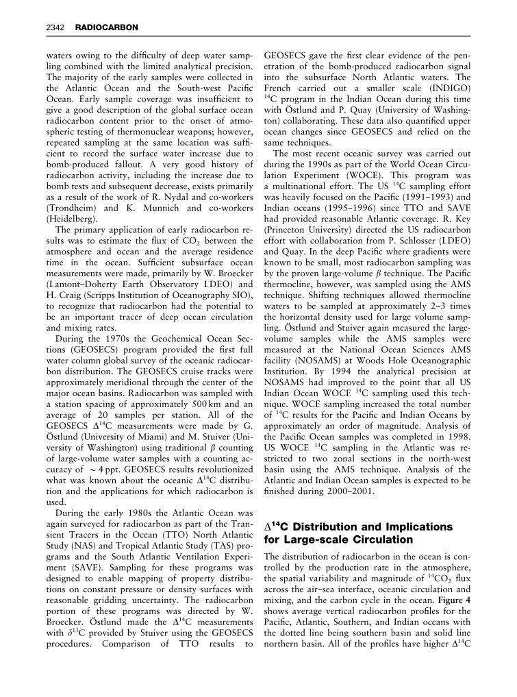
The most recent oceanic survey was carried outduring the 1990s as part of the World Ocean Circu-lation Experiment (WOCE). This program wasa multinational effort. The US 14C sampling effortwas heavily focused on the PaciRc (1991}1993) andIndian oceans (1995}1996) since TTO and SAVEhad provided reasonable Atlantic coverage. R. Key(Princeton University) directed the US radiocarboneffort with collaboration from P. Schlosser (LDEO)and Quay. In the deep PaciRc where gradients wereknown to be small, most radiocarbon sampling wasby the proven large-volume b technique. The PaciRcthermocline, however, was sampled using the AMStechnique. Shifting techniques allowed thermoclinewaters to be sampled at approximately 2}3 timesthe horizontal density used for large volume samp-ling. OG stlund and Stuiver again measured the large-volume samples while the AMS samples weremeasured at the National Ocean Sciences AMSfacility (NOSAMS) at Woods Hole OceanographicInstitution. By 1994 the analytical precision atNOSAMS had improved to the point that all USIndian Ocean WOCE 14C sampling used this tech-nique. WOCE sampling increased the total numberof 14C results for the PaciRc and Indian Oceans byapproximately an order of magnitude. Analysis ofthe PaciRc Ocean samples was completed in 1998.US WOCE 14C sampling in the Atlantic was re-stricted to two zonal sections in the north-westbasin using the AMS technique. Analysis of theAtlantic and Indian Ocean samples is expected to beRnished during 2000}2001.

*14C Distribution and Implicationsfor Large-scale Circulation

The distribution of radiocarbon in the ocean is con-trolled by the production rate in the atmosphere,the spatial variability and magnitude of 14CO2 Suxacross the air}sea interface, oceanic circulation andmixing, and the carbon cycle in the ocean. Figure 4shows average vertical radiocarbon proRles for thePaciRc, Atlantic, Southern, and Indian oceans withthe dotted line being southern basin and solid linenorthern basin. All of the proRles have higher *14C

2342 RADIOCARBON


Atlantic

_ 200 _ 100 0 100

Indian

Pacific

Pre

ssur

e (d

B)

0

1000

2000

3000

4000

5000

6000

−200 −100 0 100

Southern

∆14C (ppt)

0

1000

2000

3000

4000

5000

6000

∆14C (ppt)

0

1000

2000

3000

4000

5000

6000

Pre

ssur

e (d

B)

0

1000

2000

3000

4000

5000

6000

−200 −100 0 100

∆14C (ppt)

−200 −100 0 100

∆14C (ppt)

Figure 4 Average vertical *14C profiles for the major ocean basins. Except for the Southern Ocean the dotted line is for theSouthern Hemisphere and the solid line for the Northern Hemisphere. The Pacific and Southern Ocean profiles were compiled fromWOCE data; the Atlantic profiles from TTO and SAVE data; and the Indian Ocean profiles from GEOSECS data. In approximatelythe upper 1000 m ("1000 dB) of each profile, the natural *14C is contaminated with bomb-produced radiocarbon.

in shallow waters, reSecting proximity to the atmo-spheric source. The different collection times com-bined with the penetration of the bomb-producedsignal into the upper thermocline negate the possi-bility of detailed comparison for the upper600}800dB (deeper for the North Atlantic). De-tailed comparison is justiRed for deeper levels. Thestrongest signal in deep and bottom waters is thatthe North Atlantic is signiRcantly younger (higher*14C) than the South Atlantic, while the oppositeholds for the PaciRc. Second, the average age of

deep water increases (*14C decreases) from Atlanticto Indian to PaciRc. Third, the Southern Ocean *14Cis very uniform below approximately 1800dB ata level (&!160 ppt). This is similar to the nearbottom water values for all three southern oceanbasins. All three differences are directly attributableto the large-scale thermohaline circulation.

Figure 5 shows meridional sections for the Atlan-tic, Indian and PaciRc oceans using subsets of thedata from Figure 4. As with Figure 4, the *14Cvalues in the upper water column have been

RADIOCARBON 2343


Latitude

Dep

th (

m)

40°S 20°S 0 20°N 40°N

5000

4000

3000

2000

1000

0

_ 150

−100

−500

50100100 150

−160

Latitude

Dep

th (

m)

60°S 40°S 20°S 0 20°N

5000

4000

3000

2000

1000

0

_150

_100_ 50

50100

−190−180−170_160

− 160

0

(A)

(B)

Latitude

Dep

th (

m)

60°S 40°S 20°S 0 20°N 40°N

5000

4000

3000

2000

1000

0

_ 200

_150_ 100

_ 500

50 100 100

_240

_230

_220_210

_190_180

_170

_160

(C)

Figure 5 Typical meridional sections for each ocean compiledfrom a subset of the data used for Figure 4. The deep watercontour patterns are primarily due to the large-scale thermo-haline circulation. The highest deep water *14C values are foundin the North Atlantic and the lowest in the North Pacific. Thenatural *14C in the upper ocean is contaminated by the influx ofbomb-produced radiocarbon.

increased by invasion of the bomb signal. The pat-tern of these contours, however, is generally repre-sentative of the natural *14C signal. The *14C"

!100& contour can be taken as the approximatedemarcation between the bomb-contaminatedwaters and those having only natural radiocarbon.

Comparison of the major features in each sectionshows that the meridional *14C distributions in thePaciRc and Indian Oceans are quite similar. Thegreatest difference between these two is that theIndian Ocean deep water (1500}3500m) is signiR-cantly younger than PaciRc deep waters. In bothoceans:

f The near bottom water has higher *14C than theoverlying deep water.

f The deep and bottom waters have higher *14C atthe south than the north.

f The lowest *14C values are found as a tongueextending southward from the north end of thesection at a depth of &2500m.

f Deep and bottom water at the south end of eachsection is relatively uniform with *14C&!160 ppt.

f The *14C gradient with latitude from south tonorth is approximately the same for both deepwaters and for bottom waters.

f The *14C contours in the thermocline shoal bothat the equator and high latitudes. (This feature issuppressed in the North Indian Ocean owing tothe limited geographic extent and the inSuence ofSows through the Indonesian Seas region andfrom the Arabian Sea.)

In the Atlantic Ocean the pattern in the shallowwater down through the upper thermocline is sim-ilar to that in the other oceans. The *14C distribu-tion in the deep and bottom waters of the Atlanticis, however, radically different. The only similaritiesto the other oceans are (1) the *14C value for deepand bottom water at the southern end of the sec-tion, (2) a southward-pointing tongue in deep water,and (3) the apparent northward Sow indicated bythe near-bottom tongue-shaped contour. Atlanticdeep water has higher *14C than the bottom water,and the deep and bottom waters at the north end ofthe section have higher rather that lower *14C asfound in the Indian and PaciRc. Additionally, the farNorth Atlantic deep and bottom waters have rela-tively uniform values rather than a strong verticalgradient.

The reversal of the Atlantic deep and bottomwater *14C gradients with latitude relative to thosein the Indian and PaciRc is due to the fact that onlythe Atlantic has the conditions of temperature andsalinity at the surface (in the Greenland}NorwegianSea and Labrador Sea areas) that allow formation ofa deep water mass (commonly referred to as NorthAtlantic Deep Water, NADW). Newly formedNADW Sows down slope from the formation regionuntil it reaches a level of neutral buoyancy. Flowis then southward, primarily as a deep western

2344 RADIOCARBON


South PacificWOCE Data at 32°S

Longitude

Dep

th (

m)

160°E 180° 160°W 140°W 120°W 100°W 80°W

6000

5000

4000

3000

2000

1000

0 ............

.

.

.

.

......

.

.

.

.

.

.

.

.

.

.

.

.

.

.

.

.

.

.

.

.

.

.

.

.

..

...............

.

.

.

.

.

.

.

.

.

.

.

.

.

.

.

.

.

..........

.

.

.

.

.

.

...

...

.

.

.

.

.

.

........

.

.

.

.

...................

.....

....

.....

.

.

..

.............

.

.

.

.

.

.

.

.

.

.

............

....

........

.........

.

.

.

.

.

.

.............

...

.....

......

.

.

.

.

.

.

.

.

.

.

.

.

.

.

.

.

.

.

.

.

.

.

.

.

.

.

.

.

.

.

..........

.

.

.

.

.

.

.

.

.

.

.

.

.

.

.

.

.

.

.

.

.

.

.

.

.

.

.

.

.

.

.

.

.

.

.

............

.

.

.

.

.

.

.

.

.

.

.

.

.

.

.

..

...

.....

.

.

.

.

.

.

.

.

.

.

.

.

.

.

.

.

.

.

.

.....

...

.

.

.

.

.

.

.

.

.

.

.

.

.

.

.

.

.

.

.

.

.

........

..

.

.

.

.

.

.

.

.

.

.

.

.

.

.

.

.

.

............

.

.

.

.

.

.

.

.

.

.

.

.

.

.

.

.

.

.

.

.

............

.

.

.

.

......

.........

.

.

.

.

.

.

.

.

.

.

.

.

.

.

.

.

.

................

.....

.......

.

.

.

.

.

.

.

.

.

.

.

.

..

..

..........

......

..........

...

.

.

...

.

.

.

.

.

.

..........

.

..

.

......

........

..

.

.

.

.

.

.

.

.........

..

.

.

.

.

.

....................

.

..

.

.

.

.

.

.

.

.

.

.......

..

.

.

.

.

.

.

..............

.

...

..

..

.

.

.

.

.

.

.

.

.

.

.....

.

.....

.

.

.

.

.

...........

.

.

.

.

.

......

..

.....

.

.

.....................

.

.

.

.

.

.

.

.

.

.

.

.....

...

.

.

.

.

.

.......

..

.

....

.

.

...............

.

.

....

..

.

.

.

.

.....

..

.

.

.

.

.

.

.

.

...

...

.

.

.

.

.

..

.

.

.

......

.

.

.

.

.

.

.

.

.

.

....

.

.

..

.

.

.

.

.

....

.

.

.

..

.

.

.

...

.

.

.

.

.

.

....

.

.........

.

.

..

.

.

.

.

.

.

.

.

.

.

.

.

.

.

.

.

_200

_200

_150_100

_ 500

50 100

_220_210

_210

_190_180

_170

_160

_160

_190_180_170

_160

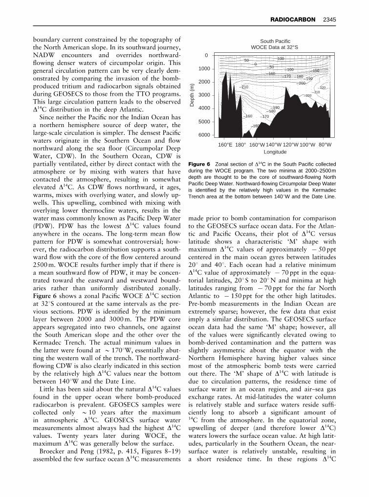
Figure 6 Zonal section of *14C in the South Pacific collectedduring the WOCE program. The two minima at 2000}2500mdepth are thought to be the core of southward-flowing NorthPacific Deep Water. Northward-flowing Circumpolar Deep Wateris identified by the relatively high values in the KermadecTrench area at the bottom between 1403W and the Date Line.

boundary current constrained by the topography ofthe North American slope. In its southward journey,NADW encounters and overrides northward-Sowing denser waters of circumpolar origin. Thisgeneral circulation pattern can be very clearly dem-onstrated by comparing the invasion of the bomb-produced tritium and radiocarbon signals obtainedduring GEOSECS to those from the TTO programs.This large circulation pattern leads to the observed*14C distribution in the deep Atlantic.

Since neither the PaciRc nor the Indian Ocean hasa northern hemisphere source of deep water, thelarge-scale circulation is simpler. The densest PaciRcwaters originate in the Southern Ocean and Sownorthward along the sea Soor (Circumpolar DeepWater, CDW). In the Southern Ocean, CDW ispartially ventilated, either by direct contact with theatmosphere or by mixing with waters that havecontacted the atmosphere, resulting in somewhatelevated *14C. As CDW Sows northward, it ages,warms, mixes with overlying water, and slowly up-wells. This upwelling, combined with mixing withoverlying lower thermocline waters, results in thewater mass commonly known as PaciRc Deep Water(PDW). PDW has the lowest *14C values foundanywhere in the oceans. The long-term mean Sowpattern for PDW is somewhat controversial; how-ever, the radiocarbon distribution supports a south-ward Sow with the core of the Sow centered around2500 m. WOCE results further imply that if there isa mean southward Sow of PDW, it may be concen-trated toward the eastward and westward bound-aries rather than uniformly distributed zonally.Figure 6 shows a zonal PaciRc WOCE *14C sectionat 323S contoured at the same intervals as the pre-vious sections. PDW is identiRed by the minimumlayer between 2000 and 3000 m. The PDW coreappears segregated into two channels, one againstthe South American slope and the other over theKermadec Trench. The actual minimum values inthe latter were found at &1703W, essentially abut-ting the western wall of the trench. The northward-Sowing CDW is also clearly indicated in this sectionby the relatively high *14C values near the bottombetween 1403W and the Date Line.

Little has been said about the natural *14C valuesfound in the upper ocean where bomb-producedradiocarbon is prevalent. GEOSECS samples werecollected only &10 years after the maximumin atmospheric *14C. GEOSECS surface watermeasurements almost always had the highest *14Cvalues. Twenty years later during WOCE, themaximum *14C was generally below the surface.

Broecker and Peng (1982, p. 415, Figures 8}19)assembled the few surface ocean *14C measurements

made prior to bomb contamination for comparisonto the GEOSECS surface ocean data. For the Atlan-tic and PaciRc Oceans, their plot of *14C versuslatitude shows a characteristic ‘M’ shape withmaximum *14C values of approximately !50 pptcentered in the main ocean gyres between latitudes203 and 403. Each ocean had a relative minimum*14C value of approximately !70 ppt in the equa-torial latitudes, 203S to 203N and minima at highlatitudes ranging from !70 ppt for the far NorthAtlantic to !150 ppt for the other high latitudes.Pre-bomb measurements in the Indian Ocean areextremely sparse; however, the few data that existimply a similar distribution. The GEOSECS surfaceocean data had the same ‘M’ shape; however, allof the values were signiRcantly elevated owing tobomb-derived contamination and the pattern wasslightly asymmetric about the equator with theNorthern Hemisphere having higher values sincemost of the atmospheric bomb tests were carriedout there. The ‘M’ shape of *14C with latitude isdue to circulation patterns, the residence time ofsurface water in an ocean region, and air}sea gasexchange rates. At mid-latitudes the water columnis relatively stable and surface waters reside sufR-ciently long to absorb a signiRcant amount of14C from the atmosphere. In the equatorial zone,upwelling of deeper (and therefore lower *14C)waters lowers the surface ocean value. At high latit-udes, particularly in the Southern Ocean, the near-surface water is relatively unstable, resulting ina short residence time. In these regions *14C

RADIOCARBON 2345


GEOSECS 1973 1974−WOCE 1992 1995−_100

0

100

200

80°S 60°S 40°S 20°S 20°N 40°N 60°N

Latitude

0°

∆14C

(pp

t)

Figure 7 Distribution of *14C in the surface Pacific Ocean asrecorded by the GEOSECS program in the early 1970s and theWOCE program in the early 1990s. From Figure 3B it followsthat GEOSECS recorded the maximum bomb-contamination.Over the 20 years separating the programs, mixing and advec-tion dispersed the signal. By the time of WOCE the maximumcontamination level was found below the surface at many loca-tions. The asymmetry about the Equator in the GEOSECS datais a result of most atmospheric bomb tests being executed inthe Northern Hemisphere.

_ 200_150

_100

_50050100 100150•

••••••••

•

••••••••••

•

•

•••

•

•

•

•

••••••••

••••

•••

•

•

•

•

•

•••••••••

•

•

••••

•

•

•

•

•

•••••••

•

•

•

••••••

••

••

•

•••••••••

•

•••••••

••

•

••••••••

•

•

••••

•

•

•

•••••••••

•

•

•

•••••••••

•

•

•••• •

••••••

•

•

•

••••••

•

•

•

•

•••••••

•

•

••••

•

•

•

•

••••

•••••••

•

•

•

•

•

•

•

•

•

•••••••

•

•

•

•

•••

•••

•

•

•

•••••••

•

••

•

•••••

•

•

•

•

••••••••

•

•

•

••••••

•

•

•

•

•

••••

•

•

•

•

•••••

•

•

_200_150 _150

_100

_100

_50050100 100

•••••••

•

•

•

•

•••••••

••

•

•

•

••••••••••••••••••

••••••••

•

•

•

•

•••••••••••••••

•

•••••••

•••

•

••••••••••••

•

•

••••••••••••••••

••

••

•

•

•

•

•

•••••

•

•

••

•••••

•

•••••••••••••••

•••••••

••

•

•••

•

•

•

•

••••••

•••••••

•

•

•

••

•••••

•

••••••••

••

•

••••••••

•

•••••••••

•

•

•

•

•••••••

•••

•

•

••••

••••

•

•

•••••••••••

•

•••••••••••••••

•

••••••••••••

•

••••••••••••••••••••

•

•

••••••••••••••

•

•••••••••••••••••••

••••••••••••••••••

•

•••••••••••••••••

•

••••••••••••••••

••

••••••••••••

•

••••••••••••

•

•

•••••••••••••

•

••

•

•••••••••••••

•

•

••••••••••••

•

•

••••••••••••••

•

••••••••••••

•

•

••••••••

••

•

•

••••••••••••

•

•

••••••••••••••

•

••••••••••••••

•

••

••••••••••••••

•

•••••••••••

•

••

•••••••••••••

•

•••••••••••••••

•

•

•

•

•••••••••

•

•

•••••••••••••••

••••••••••••

••

••

••••••••••••

•

•

•

•

•

••

••••••

•••••

••

••••

••••

••••

••

••

•••••••••••••

••

•••••

••••••••

••

•••••••

•••

••

••

••

••••

•••••••

••

•••••••••••••••••

••

•••••••••••••••••••

••

••••••••••••

•

••••••••••

•

•

•••••••••••

•••

••

•

•••••••

Latitude

Dep

th (

m)

60°S 40°S 20°S 0° 20°N 40°N 60°N

1200

600

200_ 75

_50 _ 50

_ 25

_25 _25

0 0

025

25 2550

50 50

60°S 40°S 20°S 0° 20°N 40°N 60°N

60°S 40°S 20°S 0° 20°N 40°N 60°N

Dep

th (

m)

1200

600

200

Dep

th (

m)

1200

600

200

(A)

(B)

(C)

1000

800

400

0

1000

800

400

0

1000

800

400

0

Figure 8 Panel (C) shows the change in the meridionaleastern Pacific thermocline distribution of *14C between theGEOSECS (1973}1974, (A)) and WOCE (1991}1994, (B)) sur-veys. The change was computed by gridding each section thenfinding the difference. The dashed lines in (C) indicate constantpotential density surfaces. Negative near-surface values indi-cate maximum concentration surfaces moving down into thethermocline after GEOSECS. The region of greatest increase inthe southern hemisphere is ventilated in the Southern Ocean.

acquired from the atmosphere is more than compen-sated by upwelling, mixing, and convection.

Figure 7 shows a comparison for GEOSECS andWOCE surface data from the PaciRc Ocean. TheGEOSECS *14C values are higher than WOCEeverywhere except for the Equator. The difference isdue to two factors. First, GEOSECS sampling occur-red shortly after the atmospheric maximum. At thattime the air}sea *14C gradient was large andthe surface ocean *14C values were dominated byair}sea gas exchange processes. Second, by the1990s, atmospheric *14C levels had declined signiR-cantly and sufRcient time had occurred for oceanmixing to compete with air}sea exchange in termsof controlling the surface ocean values. Duringthe 1990s, the maximum oceanic *14C values werefrequently below the surface. Near the Equatorthe situation is different. SigniRcant upwelling oc-curs in this zone. During GEOSECS, waters upwell-ing at low latitude in the PaciRc were not yetcontaminated with bomb radiocarbon. Twentyyears later, the upwelling waters had acquireda bomb radiocarbon component.

While surface ocean *14C generally decreasedbetween GEOSECS and WOCE, values throughoutthe upper kilometer of the water column generallyincreased as mixing and advection carried bomb-produced radiocarbon into the upper thermocline.The result of these processes on the bomb-produced*14C signal can be visualized by comparingGEOSECS and WOCE depth distributions. Figure 8shows such a comparison. To produce this Rgure

the WOCE data from section P16 (1523W) weregridded (center panel). GEOSECS data collectedeast of the data line were then gridded to the samegrid (top panel). Once prepared, the two sectionswere simply subtracted grid box by grid box(bottom panel). One feature of Figure 8 is theasymmetry about the Equator. The difference at thesurface in Figure 8 reSects the same information(and data) as in Figure 7. The greatest increase (upto 60 ppt) along the section is in the SouthernHemisphere mid-latitude thermocline at a depth of300}800m. This concentration change decreases inboth depth and magnitude toward the Equator. Allof the potential density isolines that pass throughthis region of signiRcant increase (dashed lines in thebottom panel) outcrop in the Southern Ocean.These outcrops (especially during austral winter)provide the primary pathway by which radiocarbonis entering the South PaciRc thermocline. In the

2346 RADIOCARBON


Silicate ( mol kg )µ_1

0 50 100 150

AtlanticPacificIndian

2350 2400 2450 2500

AtlanticPacificIndian

∆14C

(pp

t)∆14

C (

ppt)

(A)

(B) Potential alkalinity, PALK ( mol kg )µ_1

_250

_150

_ 50

_250

_150

_ 50

_ 200

_ 100

_200

_100

Figure 9 Comparison of the correlation of natural *14Cwith silicate (A) and potential alkalinity (PALK"[alkalinity#nitrate]]35/salinity) (B) using the GEOSECS global data.Samples from high southern latitudes are excluded from thesilicate relation. The presence of tritium was used to surmise thepresence of bomb-*14C. The somewhat anomalous high PALKvalues from the Indian Ocean are from upwelling}high produc-tivity zones and may be influenced by nitrogen fixation and/orparticle flux.

North PaciRc the surface ocean decrease extends asa blob well into the water column ('200 m). Thislarge change is due to the extremely high surfaceconcentrations measured during GEOSECS and tosubsurface mixing and ventilation processes thathave diluted or dispersed the peak signal. The valuescontoured in the bottom panel represent the changein *14C between the two surveys, not the total bomb*14C.

WOCE results from the Indian Ocean are not yetavailable. Once they are, changes since GEOSECS inthe South Indian Ocean should be quite similar tothose in the South PaciRc because the circulationand ventilation pathways are similar. Changes in theNorth Indian Ocean are difRcult to predict owing towater inputs from the Red Sea and the IndonesianthroughSow region and to the changing monsoonalcirculation patterns.

GoK te OG stlund and Claes Rooth describedradiocarbon changes in the North Atlantic Oceanusing data from GEOSECS (1972) and the TTONorth Atlantic Study (1981}1983). The pattern ofchange they noted is different from that in the Paci-Rc because of the difference in thermohaline circula-tion mentioned previously. Prior to sinking, theformation waters for NADW are at the ocean sur-face long enough to pick up signiRcant amounts ofbomb radiocarbon from the atmosphere. The circu-lation pattern coupled with the timing of GEOSECSand TTO sampling resulted in increased *14C levelsduring the latter program. The signiRcant changeswere mostly limited to the deep water region northof 403N latitude. When the WOCE Atlantic samplesare analyzed, we expect to see changes extendingfarther southward.

Separating the Natural and BombComponents

Up to this point the discussion has been limited tochanges in radiocarbon distribution due to oceanicuptake of bomb-produced radiocarbon. Manyradiocarbon applications, however, require not thechange but the distribution of either bomb or natu-ral radiocarbon. Ocean water measurements givethe total of natural plus bomb-produced *14C. Sincethese two are chemically and physically identical, noanalytical procedure can differentiate one from theother. Far too few *14C measurements were madein the upper ocean prior to contamination by thebomb component for us to know what the upperocean natural *14C distribution was.

One separation approach derived by Broecker andco-workers at LDEO uses the fact that *14C is

linearly anticorrelated with silicate in waters belowthe depth of bomb-14C penetration. By assumingthe same correlation extends to shallow waters, thenatural *14C can be estimated for upper thermoclineand near surface water. Pre-bomb values for theocean surface were approximated from the few pre-bomb surface ocean measurements. The silicatemethod is limited to temperate and low-latitudewaters since the correlation fails at high latitudes,especially for waters of high silicate concentration.More recent work by S. Rubin and R. Key indicatesthat potential alkalinity (alkalinity#nitrate nor-malized to salinity of 35) may be a better co-vari-able than silicate and can be used at all latitudes.Figure 9 illustrates the silicate and PALK correla-tions using the GEOSECS data set. Regardless of theco-variable, the correlation is used to estimate pre-bomb *14C in contaminated regions. The differencebetween the measured and estimated natural *14C isthe bomb-produced *14C.

RADIOCARBON 2347


Dep

th (

m)

_ 200 _100 0 100

2000

1000

0

MeasuredPALK estimateSilicate estimate

Dep

th (

m)

0 50 100 150 200

2000

1000

0

PALK estimateSilicate estimate

(A)

(B)

1500

500

1500

500

∆14C (ppt)

Bomb C (ppt)∆14

Figure 10 Panel (A) compares measured *14C from a mid-latitude Pacific WOCE station with natural *14C estimated usingthe silicate and potential alkalinity methods. Bomb-*14C, thedifference between measured and natural *14C, estimated withboth methods is compared in (B). Integration of estimatedbomb-*14C from the surface down to the depth where theestimate approaches zero yields an estimate of the bomb-*14Cinventory. Inventory is generally expressed in units of atoms perunit area.

In Figure 10 the silicate and potential alkalinity(PALK) methods are illustrated and compared. Theupper panel (A) shows the measured *14C and esti-mates of the natural *14C using both methods. Thebomb *14C is then just the difference between themeasured value and the estimate of the naturalvalue (B). For this example, taken from the mid-latitude PaciRc, the two estimates are quite close;however this is not always true.

In Figure 11A the upper 1000 m of the PaciRcWOCE *14C section shown in Figure 5C is repro-duced. Figure 11B shows the estimated natural *14Cusing the potential alkalinity method. The shape ofthe two contour sets is quite similar; however, thecontour values and vertical gradients are very differ-ent, illustrating the strong inSuence of bomb-produced radiocarbon on the upper ocean. The in-tegrated difference between these two sectionswould yield an estimate of the bomb-produced *14Cinventory for the section.

Oceanographic Applications

As illustrated, the *14C distribution can be used toinfer general large-scale circulation patterns. Themost valuable applications for radiocarbon derivefrom the fact that it is radioactive and has a half-lifeappropriate to the study of deep ocean processesand that the bomb component is transient and isuseful as a tracer for upper ocean processes. A fewof the more common uses are described below.

Deep Ocean Mixing and VentilationRate and Residence Time

Since the Rrst subsurface measurements of radiocar-bon, one of the primary applications has been thedetermination of deep ocean ventilation rates. Mostof these calculations have used a box model toapproximate the ocean system. The Rrst suchestimates yielded mean residence times for thevarious deep and abyssal ocean basins of 350}900years. Solution of these models generally assumesa steady-state circulation, identiRable source waterregions with known *14C, no mixing between watermasses, and no signiRcant biological sources orsinks. Another early approach assumed that thevertical distribution of radiocarbon in the deep andabyssal ocean could be described by a vertical ad-vection}diffusion equation. This type of calculationleads to estimates of the effect of biological particleSux and dissolution and to the vertical upwellingand diffusion rates. The 1D vertical advection}diffu-sion approach has been abandoned for 2D and 3Dcalculations as the available data and our knowl-edge of oceanic processes have increased.

When the GEOSECS data became available, boxmodels were again used to estimate residence timesand mass Suxes for the abyssal ocean. In this casethe model had only four boxes, one for the deepregion ('1500m) of each ocean. New bottomwater formation (NADW and Antarctic BottomWater, AABW) were included as inputs to theAtlantic and Circumpolar boxes. Upwelling was al-lowed in the Atlantic, PaciRc, and Indian boxes andexchange was considered between the Circumpolarbox and each of the other three ocean boxes. Re-sults from this calculation gave mean replacementtimes of 510, 250, 275, and 85 years for the deepPaciRc, Indian, Atlantic, and Southern Ocean, re-spectively, and 500 years for the deep waters of theentire world. Upwelling rates were estimated at4}5 m y~1 and mass transports generally agreed withcontemporary geostrophic calculations. Applyingthe same model to more recent data sets would yieldthe same results.

2348 RADIOCARBON


Latitude

Dep

th (

m)

60°S

60°S

40°S

40°S

20°S

20°S

0

0

20°N

20°N

40°N

40°N

60°N

60°N

1000

600

200

0 ...........

.

.

.

..

.

.

.

.

.

....

.

.

.

.

.

.......

.

.

.

.

......

....

.

.

.

.

.

.

.

.

.

.

....

.

.

.

.

......

.

.

.

.

.

.

.

....

.

..

.

.

.

..

.

.

.

....

.

.

.

.

......

.

.

.

.

.

....

.

.

.

.

.

.

.

.

.

.

.

.

.

..

.

.

.

.

.......

.

.

.

.

.

.

.

.

...

.

.

.

.

.

.

.

.

.

.

.

.

.

...

.

.

.

.

.

.

.

.

.

.

.

.

.

.

.

.

..

.

..

.

.

.

.

.

.

.

.

.

.

.

.

.

.

...

..

.

.

.

.

....

..

.

.

.

.

.

..

.

.

.

..

.

.

.

.

......

.

.

.

.

.

...

....

.

..

.

.

.

.

.

...

..

...

.

.

.

..............

.

.

.

.

.

. .

..........

.

.

.

.

.............

.

.

.

.

............

.

.

.

.

..

..............

.

.

.

...

........

.

.

.

.

.

.....

......

.

.

........

...

.

.

.............

.

.

.............

.

.....

.......

.

...........

.

.

.

.

......

.....

.

.

........

.

.

............

.

............

.

.

.............

.

.

.

.........

.

.

.

.

.

........

.

.

.

.

.

........

.

.

.

.

.

............

.

.

.

..

.

.

..

.....

.

.

....

.....

.

.

.

.

.

.

............

..

.

.

.

.

.

.

.

.

.

.

.

.

...

..

.

.

.

.

.

.

...

.

.

..

.

.

..

.

.....

..

.

.

.

.

.

.....

....

.

..

.

..

.

......

..

.

..

.

.

.

...

.

.

.

.

.

.

.

..

........

.

..

.

...

.

.............

..

..

..

.

............

.

.

.

.

........

.

.

.

.

.

.

.

....

.

.

.

.

.

.

.

.....

.

.

.

.

.

.

............

.

.

.

._ 200_160

_120

_80_ 40

0

40

80100 100

Latitude

........

.

.

.

.

.....

...

.

.

.

.

....

...................

...............

...........

....

.

.

.

.

....................

....................

................

.................

..

.

...

.........

.

..

.

.

...................

.................

.................

.....

..

.

.

.

.

.

.

.........

.

.

.

.

.

..........

.

.

.

.

.

.

...................

...

.

.

.

.

.

.

.........

.

.

.

.

.

.

.

..

.........

.

.

.

.

................

...................

.................

...................

....................

...............

.

.

.

....................

...................

............

.

.

.

.

.

..............

.

.

.

...................

...................

..............

.

.

.

.

.

.

..................

.

...........

.

.

............

.

.

.

...

...............

.

.

............

.

.

.

.............

.

.

.

.

...............

.

.

.

...............

.

.

................

.

.

...........

...

.

.

.

.

.................

.

.

.........

.

.

.

.

.

.

..............

.

.

.

............

.

.

.

.

.............

.

.

.

.

.........

.

.

.

.

.

.

........

.

.

.

.

.

.

........

.

.

.

.

.

.

.............

.

.

.

.

.

.

.

.....

................

.

.

.

......

.

.

..

.

.

..................

.

.

.

....

..

.

.

.

.

.

.

.

.

.

.

.

.

.

.

.

........

....

.....

.

.

.

..

..

.

.

.

..

..

.

.

.

.

.

.

.....

..

.

.

.

.

.........

............

.

..

.

...

.

.

.

.

.

.

........

..

.

.

.

...

..

.

.

.

.

.

.

...............

............

.

....

.

.

.

.

.

.

.

.......

..

.

.

.

..

.

..

.

.

.

.

.

..............

.

.

.

.

.........

........

...........

.

.

.

.

.

...

.

.......................

.

........

.......

.........

.....

.

.

.

.

.

.

.

..........

.

.

.

.

.

.

.........

.............

.

.

.

.

.........

........

_220_200_180

_160

_140_120

_100_80

_60

Dep

th (

m)

1000

600

200

0

800

400

800

400

Figure 11 Upper thermocline meridional sections along 1523W in the central Pacific. (A) The same measured data as in Figure5C. (B) An estimate of thermocline *14C values prior to the invasion of bomb-produced radiocarbon.

_240 _ 220 _ 200 _180 _160

140

160

180

200

∆14C (ppt)

App

aren

t oxy

gen

utili

zatio

n (

mol

kg

)µ

_1

Figure 12 Apparent oxygen utilization plotted against mea-sured *14C for WOCE Pacific Ocean samples taken at depthsgreater than 4000 m and north of 403S. The slope of the line(!0.831$0.015) can be used to estimate an approximateoxygen utilization rate of 0.1lmol kg~1 y~1 if steady state andno mixing with other water masses is assumed.

Oxygen Utilization Rate

Radiocarbon can be used to determine the rate ofbiological or geochemical processes such as the rateat which oxygen is consumed in deep ocean water.The simplest example of this would be the case of awater mass moving away from a source region at asteady rate, undergoing constant biological oxygenuptake and not subject to mixing. In such a situ-ation the oxygen utilization rate could be obtainedfrom the slope of oxygen versus 14C in appropriateunits. The closest approximation to this situation is

the northward transport of CDW in the abyssalPaciRc, although the mixing requirement is onlyapproximate. Figure 12 shows such a plot forWOCE PaciRc Ocean samples from deeper than4000 m and north of 403S. In this case, apparentoxygen utilization (saturated oxygen concentrationat equilibration temperature ! measured oxygenconcentration) rather than oxygen concentration isplotted, to remove the effect of temperature on oxygensolubility. The least-squares slope of 0.83lmol kg~1

per ppt converts to 0.1 lmol kg~1 y~1 for an oxygenutilization rate. Generally, mixing with other watermasses must be accounted for prior to evaluatingthe gradient. With varied or additional approxima-tions, very similar calculations have been used toestimate the mean formation rates of various deepwater masses.

Ocean General Circulation ModelCalibration

Oceanographic data are seldom of value forprediction. Additionally, the effect of a changingoceanographic parameter on another parameter canbe difRcult to discern directly from data. These re-search questions are better investigated with numer-ical ocean models. Before an ocean model result canbe taken seriously, however, the model must dem-onstrate reasonable ability to simulate current con-ditions. This generally requires that various modelinputs or variables be ‘tuned’ or calibrated to matchmeasured distributions and rates. Radiocarbon isthe only common measurement that can be used to

RADIOCARBON 2349


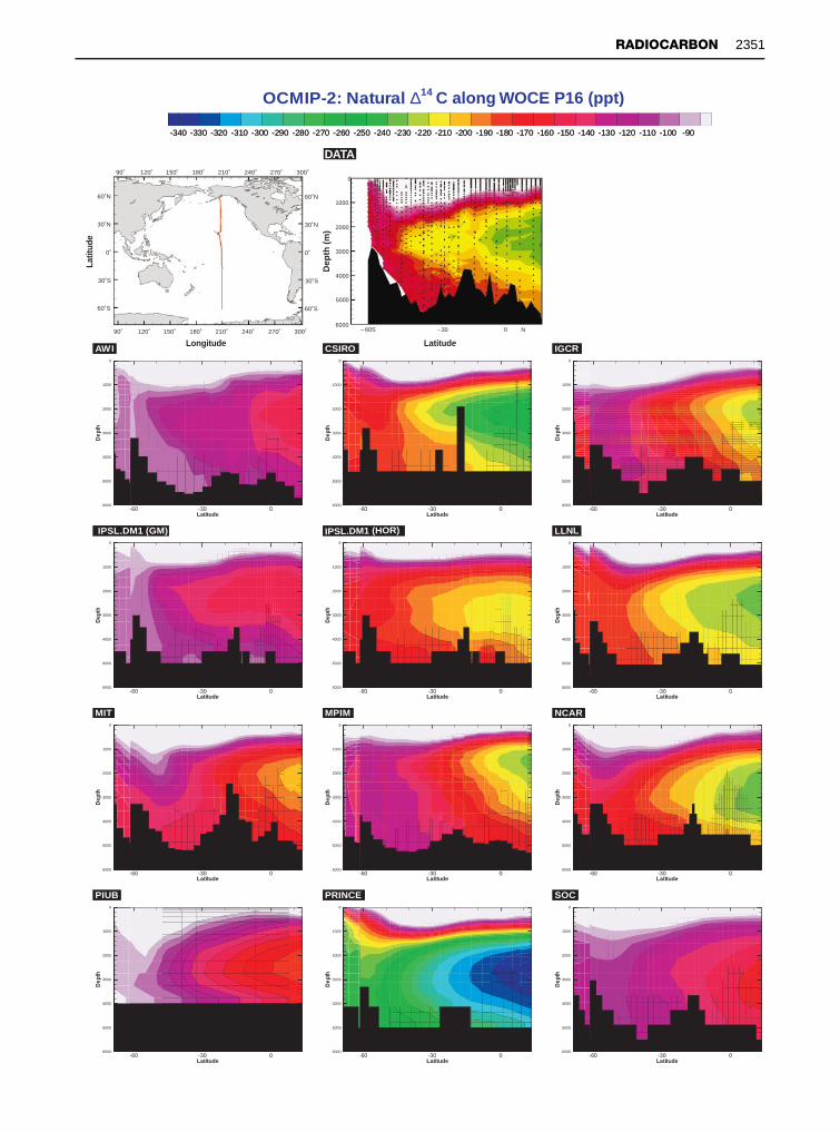
Figure 13 (Right) Global ocean circulation model results from 12 different coarse-resolution models participating in OCMIP-2compared to WOCE data for natural *14C on a meridional Pacific section. The model groups are identified in each subpanel and inTable 1. All of the models used the same chemistry and boundary conditions.

calibrate the various rates of abyssal processes ingeneral circulation models. M. Fiadeiro carried outthe Rrst numerical simulation for the abyssal PaciRcand used the GEOSECS 14C data to calibrate themodel. J.R. Toggweiler extended this study usinga global model.

Both the Fiadeiro and Toggweiler models, and allsubsequent models that include the deep water*14C, are of coarse resolution owing to currentcomputer limitations. As the much larger WOCE14C data set becomes available, the failure of thesemodels, especially in detail, becomes more evident.Toggweiler’s model, for example, has advectivemixing in the Southern Ocean that is signiRcantlygreater than supported by data. Additionally, thecoarse resolution of the model prevents the forma-tion of, or at least retards the importance of, deepwestern boundary currents. SigniRcant model deR-ciencies appear when the bomb-14C distribution andintegrals at the time of GEOSECS and WOCE arecompared with data.

During the last 10 years the number and varietyof numerical ocean models has expanded greatly,in large part because of the availability and speedof modern computers. The Ocean Carbon ModelIntercomparison Project (OCMIP) brought oceanmodelers together with data experts in the Rrstorganized effort to compare model results withdata, with the long-term goals of understanding theprocesses that cause model differences and of im-proving the prediction capabilities of the models.The unique aspect of this study was that each parti-cipating group essentially ‘froze’ development of theunderlying physics in their model and then used thesame boundary conditions and forcing in order toeliminate as many potential variables as possible.Radiocarbon, both bomb-derived and natural, wereused as tracers in each model to examine air}sea gasexchange and long-term circulation. Figure 13 com-pares results from 12 global ocean circulationmodels with WOCE data from section P16. The tagin the top left corner of each panel identiRes theinstitution of the modeling group. All of the modelresults and the data are colored and scaled identi-cally and the portion of the section containing bombradiocarbon has been masked. While all of themodels get the general shape of the contours, theconcentrations vary widely. Detailed comparison iscurrently under way, but cursory examinationpoints out signiRcant discrepancies in all modelresults and remarkable model-to-model differences.

Similar comparisons can be made focusing on thebomb component. Discussion of model differences isbeyond the scope of this work. For information, seepublications by the various groups having results inFigure 13 (listed in Table 1). These radiocarbonresults are not yet published, but an overview of theOCMIP-2 program can be found in the work ofDutay on chloroSuorocarbon in the same models(see Further Reading).

Air^Sea Gas Exchange andThermocline Ventilation Rate

Radiocarbon has been used to estimate air}sea gasexchange rates for almost as long as it has beenmeasured in the atmosphere and ocean. Generally,these calculations are based on box models, whichhave both included and excluded the inSuence ofbomb contamination. W. Broecker and T.-H. Pengsummarized efforts to estimate air}sea transfer ratesup to 1974 and gave examples based on GEOSECSresults using both natural and bomb-14C and a stag-nant Rlm model. In this, the rate-limiting step fortransfer is assumed to be molecular diffusion of thegas across a thin layer separating the mixed layer ofthe ocean from the atmosphere. In this model, if oneassumes steady state for the 14C and 12C distributionand uniform 14C/12C for the atmosphere and surfaceocean then the amount of 14C entering the oceanmust be balanced by decay. For this model thesolution is given by eqn [3].

Dz"

+ [CO2] Docean

+ [CO2] Dmix

VAC

14C/CDocean14C/CDatm D

a14CO2

aCO2

1!C14C/CDmix14C/CDatmD

a14CO2

aCO2

j [3]

Here D is the molecular diffusivity of CO2, z is theRlm thickness, a

iis the solubility of i, V and A are

the volume and surface area of the ocean, and j isthe 14C decay coefRcient. Use of pre-industrial meanconcentrations gave a global boundary layer thick-ness of 30lm (D/z&1800 m y~1

"piston velocity).The Rlm thickness is then used to estimate gas resi-dence times either in the atmosphere or in the mixedlayer of the ocean. For CO2 special considerationmust be made for the chemical speciation in theocean, and for 14CO2 further modiRcation is neces-sary for isotopic effects. The equilibration times forCO2 with respect to gas exchange, chemistry, and

2350 RADIOCARBON


-340 -330 -320 -310 -300 -290 -280 -270 -260 -250 -240 -230 -220 -210 -200 -190 -180 -170 -160 -150 -140 -130 -120 -110 -100 -90

OCMIP-2: Natural ∆14Ca long

Latitude

Dep

th

-60 -30 0

0

1000

2000

3000

4000

5000

6000

AW I

Latitude

Dep

th

-60 -30 0

0

1000

2000

3000

4000

5000

6000

CSIRO

Latitude

Dep

th

-60 -30 0

0

1000

2000

3000

4000

5000

6000

IGC

Latitude

Dep

th

-60 -30 0

0

1000

2000

3000

4000

5000

6000

LLNL

Latitude

Dep

th

-60 -30 0

0

1000

2000

3000

4000

5000

6000

NCA

Latitude

Dep

th

-60 -30 0

0

1000

2000

3000

4000

5000

6000

MP

Latitude

Dep

th

-60 -30 0

0

1000

2000

3000

4000

5000

6000

MIT

Latitude

Dep

th

-60 -30 0

0

1000

2000

3000

4000

5000

6000

PI

Latitude

Dep

th

-60 -30 0

0

1000

2000

3000

4000

5000

6000

Latitude

Dep

th

-60 -30 0

0

1000

2000

3000

4000

5000

6000

SO

Latitude

Dep

th

-60 -30 0

0

1000

2000

3000

4000

5000

6000

IPS

Latitude

Dep

th

-60 -30 0

0

1000

2000

3000

4000

5000

6000

PSL

Latitude

Dep

th

-60 -30 0

0

1000

2000

3000

4000

5000

6000

SOC

Latitude

Dep

th

-60 -30 0

0

1000

2000

3000

4000

5000

6000

NCAR

Latitude

Dep

th

-60 -30 0

0

1000

2000

3000

4000

5000

6000

MPIM

Latitude

Dep

th

-60 -30 0

0

1000

2000

3000

4000

5000

6000

PIUB

Latitude

Dep

th

-60 -30 0

0

1000

2000

3000

4000

5000

6000

PRINCE

Latitude

Dep

th

-60 -30 0

0

1000

2000

3000

4000

5000

6000

LLNL

Latitude

Dep

th

-60 -30 0

0

1000

2000

3000

4000

5000

6000

CSIRO

Latitude

Dep

th

-60 -30 0

0

1000

2000

3000

4000

5000

6000

IGCR

-340 -330 -320 -310 -300 -290 -280 -270 -260 -250 -240 -230 -220 -210 -200 -190 -180 -170 -160 -150 -140 -130 -120 -110 -100 -90

OCMIP-2: Natural ∆14

Latitude

Dep

th

-60 -30 0

0

1000

2000

3000

4000

5000

6000

IPSL.DM1 (HOR)

Latitude

Dep

th

-60 -30 0

0

1000

2000

3000

4000

5000

6000

AW I

Latitude

Dep

th

-60 -30 0

0

1000

2000

3000

4000

5000

6000

IPSL.DM1 (GM)

Latitude

Dep

th

-60 -30 0

0

1000

2000

3000

4000

5000

6000

MIT

C along WOCE P16 (pp t)

DATA

DATA

Latit

ude

90˚ 120˚ 150˚ 180˚ 210˚ 240˚ 270˚ 300˚

60˚S

30˚S

0˚

30˚N

60˚N

90˚ 120˚ 150˚ 180˚ 210˚ 240˚ 270˚ 300˚

Long itude

60˚S

30˚S

30˚N

60˚N

0˚

_ 60S _30 06000

5000

4000

3000

2000

1000

0

Dep

th (

m)

Latitude

N

RADIOCARBON 2351


Table 1 OCMIP-2 participants

Model groupsAWI Alfred Wegener Institute for Polar and Marine

Research, Bremerhaven, GermanyCSIRO Commonwealth Science and Industrial

Research Organization, Hobart, AustraliaIGCR/CCSR Institute for Global Change Research, Tokyo,

JapanIPSL Institut Pierre Simon Laplace, Paris, FranceLLNL Lawrence Livermore National Laboratory,

Livermore, CA, USAMIT Massachusetts Institute of Technology,

Cambridge, MA, USAMPIM Max Planck Institut fur Meteorologie, Hamburg,

GermanyNCAR National Center for Atmospheric Research,

Boulder, CO, USAPIUB Physics Institute, University of Bern,

SwitzerlandPRINCEton Princeton University AOS, OTL/GFDL,

Princeton, NJ, USASOC Southampton Oceanography

Centre/SUDO/Hadley Center, UK Met.Office

Data groupsPMEL Pacific Marine Environmental Laboratory,

NOAA, Seattle, WA, USAPSU Pennsylvania State University, PA, USAPRINCEton Princeton University AOS, OTL/GFDL,

Princeton, NJ, USA

•

••

• •••••••••••••••••••••

•••••

•••

•

••

••

•

••

•••

•••

•••••••• •

•••••••••

••

••

•••••••

•

••••••••••••••••••••••••••

•••

•••

•••

••

•

••

• •

•••

•

•

•••

••••

•

••

0°140°E 180°160°E 160°W 140°W 120°W 100°W 80°W

10°N

20°N

30°N

40°N

50°N

Longitude

Latit

ude

Contour lines = Bomb C (ppt)∆14

100

120

140

Figure 14 Bomb-*14C on the potential density surfaceph"26.1 in the North Pacific. The blue line is the wintertimeoutcrop of the surface based on long-term climatology. The Seaof Okhotsk is a known region of thermocline ventilation for theNorth Pacific.

Latitude

0

100

150

200

25.7526.1026.3026.5026.65

10°N 20°N 30°N 40°N 50°N

50Bom

bC

(pp

t)∆14

0°

Figure 15 Meridional distribution of bomb-*14C on potentialdensity surfaces in the North Pacific thermocline.

isotopics are approximately 1 month, 1 year, and 10years, respectively.

Radiocarbon has been used to study thermoclineventilation using tools ranging from simple 3-boxmodels to full 3D ocean circulation models. Manyof the 1D and 2D models are based on work by W.Jenkins using tritium in the North Atlantic. In arecent example, R. Sonnerup and co-workers at theUniversity of Washington used chloroSuorocarbondata to calibrate a 1D (meridional) along-isopycnaladvection}diffusion model in the North PaciRc withWOCE data. Equation [4] is the basic equation forthe model.

dCdt

"!vdCdx

#Kd2Cdx2 [4]

In eqn [4] C is concentration, K is along-isopycnaleddy diffusivity, !v is the southward componentof along isopycnal velocity, t is time, and x is themeridional distance. Upper-level isopycnal surfacesoutcrop at the surface. Once the model is calibrated,the resulting values are used to investigate the distri-bution of other parameters. The original work andthe references cited there should be read for details,but Figure 14 shows an objective map of the bomb-14C distribution on the potential density surface

26.1 for the North PaciRc and Figure 15 summarizesthe bomb-14C distribution as a function of latitude.These Rgures illustrate the type of data that wouldbe input considerations to an investigation ofthermocline ventilation.

Conclusions

Since the very earliest measurements, radiocarbonhas proven to be an extremely powerful tracer, andsometimes the only available tracer, for the study ofmany oceanographic processes. Perhaps the mostimportant of these today are large-scale deep oceanmixing and ventilation processes and the calibrationof numerical ocean models. The Rrst global surveyof the radiocarbon distribution collected on theGEOSECS program resulted in radical changes in

2352 RADIOCARBON


the way the abyssal ocean is viewed. The newer andmuch denser WOCE survey will certainly add signi-Rcant detail and precision to what is known andwill probably result in other, if not so many, totallynew discoveries. Progress with this tracer today isdue largely to the decrease in required sample sizefrom &250 liters to &250 milliliters and to theavailability and application of fast, inexpensivecomputers.

See also

Abyssal Currents. Air+Sea Gas Exchange. Atmo-spheric Input of Pollutants. Bottom Water Forma-tion. Carbon Cycle. Carbon Dioxide (CO2) Cycle.Elemental Distribution: Overview. Long-termTracer Changes. Marine Silica Cycle. OceanCarbon System, Modelling of. Ocean Subduction.Current Systems in the Indian Ocean. RadioactiveWastes. Stable Carbon Isotope Variations in theOcean. Thermohaline Circulation. Tracers andLarge Scale Models. Tritium+Helium Dating. WaterTypes and Water Masses.

Glossary

dpm Disintegrations per minute:a measure of the activity of a radio-active substance frequently usedrather than concentration.

t1@2Half-life: time required for one halfof the atoms of a radioactive spe-cies to decay.

k Decay constant for a radioactivespecies"ln(2)/t1@2

.Mean life, j~1 Average time expected for a given

radioactive atom to decay.Abyssal Very deep ocean, often near bot-

tom.Steady state Unchanging situation over long

time interval relative to the processunder consideration; frequentlyassumed state for the deep andabyssal ocean with respect to manyparameters.

Further ReadingBroecker WS, Gerard R, Ewing M and Heezen BC (1960)

Natural radiocarbon in the Atlantic Ocean. Journal ofGeophysical Research 65(a): 2903}2931.

Broecker WS and Peng T-H (1974) Gas exchange ratesbetween air and sea. Tellus 26: 21}34.

Broecker WS and Peng T-H (1982) Tracers in the Sea.Columbia University, Palisades, NY: Lamont-DohertyGeological Observatory.

Broecker WS, Sutherland S, Smethie W, Peng T-H andOG stlund G (1995) Oceanic radiocarbon: separation ofnatural and bomb components. Global BiogeochemicalCycles 9(2): 263}288.

Craig H (1969) Abyssal carbon radiocarbon in thePaciRc. Journal of Geophysical Research 74(23):5491}5506.

Druffel, ERM and GrifRn S (1999) Variability of surfaceocean radiocarbon and stable isotopes in the south-western PaciRc. Journal of Geophysical Research104(C10): 23607}23614.

Dutay JC, Bullister JL, Doney SC et al. (2001) Evaluationof ocean model ventilation with CFC-11: comparisonof 13 global ocean models. Global BiogeochemicalCycles (in press).

Fiadeiro ME (1982) Three-dimensional modeling oftracers in the deep PaciRc Ocean, II. Radiocarbonand circulation. Journal of Marine Research 40:537}550.

Key RM, Quay PD, Jones GA et al. (1996) WOCE AMSradiocarbon I: PaciRc Ocean results (P6, P16 and P17).Radiocarbon 38(3): 425}518.

Libby WF (1955) Radiocarbon Dating, 2nd edn. Chicago:University of Chicago Press.

OG stlund HG and Rooth CGH (1990) The North Atlantictritium and radiocarbon transients 1972}1983. Journalof Geophysical Research 95(C11): 20147}20165.

Schlosser P, BoK nisch G, Kromer B et al. (1995) Mid-1980sdistribution of tritium, 3He, 14C and 39Ar in theGreenland/Norwegian Seas and the Nansen Basinof the Arctic Ocean. Progress in Oceanography 35:1}28.

Sonnerup RE, Quay PD and Bullister JL (1999) Ther-mocline ventilation and oxygen utilization rates inthe subtropical North PaciRc based on CFC distribu-tions during WOCE. Deep-Sea Research I 46:777}805.

Stuiver M and Polach HA (1977) Discussion: Reportingof 14C data. Radiocarbon 19(3): 355}363.

Stuiver M and Quay P (1983) Abyssal water carbon-14distribution and the age of the World Ocean. Science219: 849}851.

Taylor RE, Long A and Kra RS (eds) (1992) RadiocarbonAfter Four Decades, An Interdisciplinary Perspective.New York: Springer.

Toggweiler JR, Dixon K and Bryan K (1989) Simulationsof radiocarbon in a coarse-resolution World Oceanmodel. 1. Steady state prebomb distributions. Journalof Geophysical Research 94(C6): 8217}8242.

RADIOCARBON 2353


radiocarbon - geophysical fluid dynamics laboratory · pdf filea constant atmospheric...

Documents