r package doe.base for factorial experiments
TRANSCRIPT

JSS Journal of Statistical SoftwareJune 2018, Volume 85, Issue 5. doi: 10.18637/jss.v085.i05
R Package DoE.base for Factorial Experiments
Ulrike GrömpingBeuth University of Applied Sciences Berlin
Abstract
The R package DoE.base can be used for creating full factorial designs and generalfactorial experiments based on orthogonal arrays. Besides design creation, some analysisfunctionality is also available, particularly (augmented) half-normal effects plots. In addi-tion to this specific functionality, the package provides convenience features for analyzingexperimental designs and the infrastructure for a suite of further packages on designingand analyzing experiments. This infrastructure is available for use also by further designof experiments packages.
Keywords: design of experiments, DoE, factorial designs, DoE.base.
1. IntroductionFactorial experiments are very common in industrial experimentation. The most widelyspread such experiments use 2-level factors only, but experiments with mixed level factorsare also quite common, for example with the 18 run experimental plan proposed by Taguchi(NIST/SEMATECH 2012). The design and execution of such experiments is often done dur-ing everyday work without support from a statistical expert – thus it is important to have asoftware available that can be safely used by non-experts. At the same time, statisticians areoften involved in the more important industrial experiments, and there are many facets toconstruction of such experiments for which a statistician very much appreciates support froma powerful software. The R package DoE.base (Grömping 2018b) targets both non-expertsand statisticians. It is part of a larger package suite containing also the packages FrF2,DoE.wrapper and RcmdrPlugin.DoE, and a fifth supporting package FrF2.catlg128 (Grömp-ing 2011b, 2013, 2017b, 2014b,c). All these packages and all packages on which DoE.basedepends (Chasalow 2012; Venables 2013; Venables and Ripley 2002; Meyer, Zeileis, and Hornik2006; Sarkar 2008) are available from the Comprehensive R Archive Network (CRAN), whichalso holds the software R itself (R Development Core Team 2018). The graphical user inter-face (GUI) package RcmdrPlugin.DoE, which will not be described in this article, providesaccess to some functionality from the package suite. Grömping (2011b) gives a detailed

2 DoE.base for Factorial Experiments in R
example-based tutorial for using it. Package DoE.base provides the infrastructure for theentire package suite, in particular the class ‘design’, functions for importing and exportingexperimental designs, and simple analysis functions for printing, summarizing, plotting, andmodeling design data.Besides providing infrastructure, the main contribution of package DoE.base is to offer fea-tures for creating factorial designs: Potentially blocked full factorials (function fac.design)and catalog-based general factorials (function oa.design) are available. The two functionsfac.design and oa.design have taken inspiration from the “white book” (Chambers andHastie 1984), where these S functions are described that never made it into base R. Themost advanced contributions of the package are the features around orthogonal arrays (func-tion oa.design), which are subject to ongoing research. These rely heavily on a catalogof orthogonal arrays, most of which have been taken from Kuhfeld (2010). To the author’sknowledge, the package is the only place in R where non-regular orthogonal arrays other thanPlackett-Burman designs are provided for experimentation. Non-regularity of an array hasbeen discussed to be beneficial for screening experiments because it implies good projectivityproperties (see, e.g., Box and Tyssedal 1996; Deng and Tang 1999; Tang and Deng 1999).This discussion has so far focused on 2-level designs, but should analogously apply to moregeneral factorial designs.There is another R package closely related to the design creation functionality of packageDoE.base: The R package planor (Kobilinsky, Bouvier, and Monod 2018) can create regularfractional factorial designs in a general sense (see also Kobilinsky, Monod, and Bailey 2017).Package DoE.base is more general than package planor in that it also creates non-regulardesigns, can calculate various types of quality criteria, and does not require specification of amodel but can optimize a design with respect to model robustness criteria. It is less generalthan planor in that it does not allow to specify a model and estimable effects, i.e., it treatsall effects of the same order on an equal footing. Sections 4 and 5.3 will illustrate functionregular.design from package planor as an alternative to functions from packages DoE.baseand FrF2.The remainder of this article is organized as follows: Section 2 briefly explains and exemplifiesfull factorial designs and orthogonal arrays and explains the basic principles of experimentaldesign. Section 3 presents the mathematical background and terminology for general orthog-onal arrays and quality criteria for them. Section 4 discusses creation of full factorial designs,in particular also with the possibility of blocking them. Section 5 provides insights into usageand inspection of the orthogonal arrays implemented in package DoE.base. Section 6 discussesdesign creation and analysis tools, using the example of an experimental design in biotechnol-ogy (Vasilev, Schmitz, Grömping, Fischer, and Schillberg 2014). Section 7 describes in moredetail the half-normal plotting functionality provided by package DoE.base. Finally, a briefoverview of further developments is provided.
2. Basics
2.1. Full factorial designs and designs based on orthogonal arrays
A factorial design is an experimental plan in which k “factors” are systematically varied.The j-th factor has lj “levels”, j = 1 . . . k. If all factors have the same number of levels,

Journal of Statistical Software 3
i.e., l1 = . . . = lk, the design is called a “fixed level” or “symmetric” design, otherwise it iscalled “mixed level” or “asymmetric”. A “full factorial” design contains (a multiple of) allfactor level combinations, i.e., a multiple of l1 · . . . · lk experimental runs. In a full factorialdesign, all coefficients for an adequately coded linear model with all main effects, two-factorinteractions, . . ., up to k-factor interactions are estimable. The number of estimable effectsremains the same, regardless of the choice of adequate coding. Section 7 will discuss how thecoding affects correlation between coefficient estimates.Full factorial designs are often not feasible in the real world, if the number of factors or thenumbers of factor levels are not very small. For example, a full factorial experiment withone 2-level factor and six 3-level factors requires 1458 runs. There are several possibilitiesfor designs with fewer runs: D-optimal designs require the specification of a model to beestimated; they can be created with R packages AlgDesign or DoE.wrapper (Wheeler 2014;Grömping 2017b), but are not the topic of this article. Here, we consider experimental designsbased on orthogonal arrays: These do not require specification of a model but assume that(i) all effects of the same degree (main effect = degree 1, two-factor interaction = degree 2,etc.) are equally important and (ii) that effects of lower degree are more important than thoseof higher degree. Orthogonal array designs are often used with the intention of estimatingmain effects only; they are particularly common for qualitative factors, although they can alsobe used for quantitative factors. For a design based on an orthogonal array, each factor iscontained with the same number of times for each level, and each pair of factors is containedwith the same number of times for each pair of levels. Genizi Taguchi provided variousorthogonal arrays for engineering experimentation; one of the most-well-known ones is an18-run array for up to one 2-level factor and up to seven 3-level factors. This array can forexample be found in NIST/SEMATECH (2012), and is also contained in package DoE.base:
R> L18
A B C D E F G H1 1 1 1 1 1 1 1 12 1 1 2 2 2 2 2 23 1 1 3 3 3 3 3 34 1 2 1 1 2 2 3 35 1 2 2 2 3 3 1 16 1 2 3 3 1 1 2 27 1 3 1 2 1 3 2 38 1 3 2 3 2 1 3 19 1 3 3 1 3 2 1 210 2 1 1 3 3 2 2 111 2 1 2 1 1 3 3 212 2 1 3 2 2 1 1 313 2 2 1 2 3 1 3 214 2 2 2 3 1 2 1 315 2 2 3 1 2 3 2 116 2 3 1 3 2 3 1 217 2 3 2 1 3 1 2 318 2 3 3 2 1 2 3 1attr(,"origin")

4 DoE.base for Factorial Experiments in R
[1] "Taguchi"attr(,"class")[1] "oa" "matrix"
further attribute(s) (accessible with attr( res$value , attrname)):[1] "comment"
This small array can already accommodate the above-mentioned experiment with one 2-levelfactor and six 3-level factors. Of course, as it is very much smaller than the 1458 runs fora full factorial, there is a substantial amount of confounding built into the array. If a smallarray like the L18 is to be used, two things are very important: picking the best possiblecolumns for the design, and understanding the limitations of the resulting design. PackageDoE.base can help with both. However, except perhaps for very preliminary investigations,it will usually be preferable to use less severely confounded designs. Package DoE.base canalso help with optimizing the selection of an array and the column selection within the array.This will be demonstrated in Sections 5 and 6.Orthogonal arrays may be regular or non-regular. In the regular case, it is possible to describethe array by a few defining relations, similar to the well-known way of doing so for regularfractional factorial 2-level designs: Starting from a full factorial design in some “generating”or “base” factors, additional factors are accommodated by assigning them to interactionsbetween the base factors, which are consequently completely confounded with the new factors’main effects. This is a little more complicated for factors with more than two levels, but thegeneral principle remains the same. One complication arises from base level factors with non-prime numbers of levels; these can be decomposed into full factorials of factors with primenumbers of levels, so-called “pseudo factors”. The aforementioned catalog of arrays containsquite a few regular arrays. Regular orthogonal designs can also be created using functionregular.design from package planor.Non-regular orthogonal arrays cannot be described by defining relations. Some of the cata-loged arrays in package DoE.base are non-regular. Section 5.1 provides details on the catalogand its usage. Note that the catalog is by no means complete; in particular, it is much moredifficult to completely enumerate all orthogonal arrays than it is to enumerate all regularorthogonal arrays. Partially complete catalogs of orthogonal arrays are available, e.g., fromthe website by Eendebak and Schoen (2010) based on the algorithm described in Schoen,Eendebak, and Nguyen (2010). In many cases, the web site provides the best arrays only, ordoes not provide an array at all (in case of very large numbers of arrays). Where a numberof arrays is shown, the complete set of arrays can in principle be obtained from Eric Schoen;however, with large numbers of arrays the complete catalogs are so large that it is not easilyfeasible to work with them.
2.2. Principles of experimental designA very important principle of experimentation is replication: When comparing two differentsetups, one will usually not rely on a single instance of each setup, but will replicate eachsetup a specified number of times. This serves the purpose of making sure that differencesare only interpreted if they are sufficiently larger than can be expected from experimentalvariation. Replication is quite different from repeating measurements only: For a properreplication, all experimental settings have to be redone for each replicate. Sometimes, with

Journal of Statistical Software 5
very variable measurement devices, it may make sense not to include replications but torepeat the measurement process only. This is called “repeated measurements” and has tobe treated quite differently from proper replication. Several design generation functions ofpackages DoE.base and FrF2 offer the option replications for specifying the number ofreplications and repeat.only for indicating whether these are proper replications (default)or repeated measurements only.One of the very useful aspects of factorial experiments is implicit replication: When exper-imenting with many factors, one can often expect higher order interactions to be irrelevant.If this is the case, the degrees of freedom that would have to be dedicated to higher orderinteractions can instead be used for estimating error variation (or for accommodating furtherexperimental factors). Therefore, in factorial experimentation, one will encounter experimentswithout replicated runs.A further important principle is blocking, which can be used to control for known influentialfactors that are not of interest in themselves, like batch-to-batch variation. For an orthogonalarray design, one can simply include the block factor as an additional factor and thus has tofind an array of the desired structure. A full factorial design can be blocked without increasingthe number of runs, by allocating the degrees of freedom for the block factor to portions frominteraction effects. This functionality is implemented in function fac.design (see Section 4).Randomization means that the experimental runs are conducted in random order; it is asafeguard against bias from unknown influences. If the run order is completely randomized,all experimental runs can be treated as independent observations, and there is little risk ofsystematic bias from experimental order or unknown factors related to experimental orderor time. In real life, there are sometimes so-called randomization restrictions; for example,experimental runs may be randomized within each block only. Function fac.design allowsrandomization within blocks, while designs created with function oa.design have to be re-randomized with function rerandomize.design for using one of the factors as a block factor.Whenever proper replication is used, package DoE.base separately randomizes each replicationas though it were a block; however, it does not include a block factor for the replications. Userswho want to include a block factor for replications in the analysis can obtain such a factorusing the function getblock. Users who want to change the randomization, i.e., randomize allreplications together instead of in separate blocks, can use the function rerandomize.design.Using the [ method for the class ‘design’, users can also reorder a design according toa randomization scheme that has been worked out outside of R. Of course, whenever therandomization involves non-trivial restrictions like randomizing in meaningful blocks, theanalysis has to be conducted accordingly.
3. General orthogonal arraysThis section provides the mathematical background for general orthogonal arrays, as far asit can be helpful for using the orthogonal arrays available in R package DoE.base.
3.1. Terminology for orthogonal arraysAn array in the sense of this article is a rectangular table of numbers with n rows andk columns, like the L18 shown on p. 3. The rows correspond to experimental runs, thecolumns to experimental factors. In the cataloged arrays in DoE.base, the levels of an l-

6 DoE.base for Factorial Experiments in R
level factor are denoted by the numbers 1 . . . l. An array becomes an experimental design byallocating numbers to factor levels. The array is orthogonal, i.e., an OA, if for each pair ofcolumns each combination of levels occurs equally often. If this is the case, main effects of allfactors can be estimated separately from each other (provided, no higher order effects are inthe model).An OA is said to be of strength s, if each combination of levels occurs equally often for eachsubset of s columns. Thus, each OA is at least of strength 2. Strength of an OA is directlyrelated to resolution of an array: Resolution, denoted by roman numerals, is always one higherthan the strength, i.e., strength 2 arrays are of resolution III and so forth. For an array ofresolution III, main effects are not aliased with main effects, but can be aliased with two-factorinteractions (three factors involved); for an array of resolution IV, main effects are not aliasedwith two-factor interactions, but can be aliased with three-factor interactions, while two-factor interactions can be aliased with other two-factor interactions (four factors involved).This notion is well-known for regular fractional factorial 2-level designs, and is completelyanalogous for non-regular designs and for designs with factors at more than 2 levels or inmixed level situations. Note that a full factorial in k factors has strength k.
3.2. Generalized word length pattern and refinements
Xu and Wu (2001) introduced the generalized word length pattern (GWLP) for general or-thogonal arrays. It is an extension of the well-known word length pattern (WLP) for regularfractional factorial 2-level designs: In the latter, one starts out with a set of base factors andallocates additional factors to interactions among these (the generating contrasts). Codingall main effects model matrix columns with “−1” (one level) and “+1” (the other level), thisway of design generation causes products of model matrix columns to be either half “−1” andhalf “+1”, or constant columns. Factors, whose product of model matrix columns yields aconstant column, form a “word” together. The word length pattern is a frequency table ofword lengths. For regular fractional factorial 2-level designs, each group of c factors eitherdoes or does not form a word, i.e., contributes one or zero to the count for words of length c.This results in a word length pattern with only integer entries.In general, partial aliasing is possible. Even if there are only 2-level factors, e.g., in a Plackett-Burman design (Plackett and Burman 1946), a set of factors can contribute a fraction of aword to the GWLP count for the respective word length. Consequently, GWLP entries neednot be integers. For example, the GWLP of the L18 is
R> GWLP(L18)
0 1 2 3 4 5 6 7 81.0 0.0 0.0 28.0 52.5 52.5 70.0 33.0 6.0
The GWLP is denoted as A0, A1, A2, A3, . . . , Ak with Ac the number of generalized wordsof length c. The entry “1” for A0 is generic and does not indicate confounding. The GWLPfor orthogonal arrays and designs based on them is usually presented starting with A3, sinceorthogonality implies absence of words of lengths one or two. The GWLP coincides with theWLP for regular fractional factorial 2-level designs; for details, consult Xu and Wu (2001)themselves or Grömping (2011a) for a more accessible account. The concepts of strength andresolution directly relate to the (G)WLP: The shortest word length with a non-zero count

Journal of Statistical Software 7
is the resolution of the design, the longest word length with a zero count is the strength.Hence, the L18 has resolution III and strength 2. Note that it is not adequate to use the term“generalized resolution” here, because that term is already in use for a different concept thatis also implemented in package DoE.base (see below).The GWLP can be used for selecting a best design by comparing designs with respect totheir so-called aberration: A design is better than another one, if it has higher resolution; incase of equal resolution, a design has smaller aberration, if its number of shortest words issmaller, in case of ties, successively considering longer words until a difference is encountered.If this principle is applied to a complete set of possible designs, the best design is said tohave “generalized minimum aberration” (GMA; analogous to minimum aberration for regularfractional factorial 2-level designs). For orthogonal arrays, one seldom compares completesets of possible designs; however, the website by Eendebak and Schoen (2010) provides GMAarrays for various scenarii.The number Ac of generalized words of length c is the sum over contributions from all setsof c factors. For a set of R factors with l1 . . . lR levels in a resolution R design (equivalent tos + 1 factors in a strength s design), Grömping and Xu (2014) have shown an upper boundfor the contribution to the count AR to be min((l1 − 1), . . . , (lR − 1)), i.e., the upper boundfor the number of generalized words in a set of R factors depends on the pattern of levels inthe set and is given by the main effect degrees of freedom for the factor with the fewest levels(the analogous result for symmetric designs was shown earlier by Xu, Cheng, and Wu 2004).Furthermore, Grömping and Xu (2014) provided a statistical rationale for the contributionsof sets of R factors to AR in resolution R designs, i.e., the building blocks for the numberof shortest words: Each R-set contribution can be seen as the sum of R2 values from linearmodels explaining orthogonal contrast columns for any one of the R factors by a full modelin the other R− 1 factors (provided the factor to be explained has orthogonally coded modelmatrix columns; otherwise, R2 values have to be replaced by squared canonical correlations).Thus, the number of shortest words measures the extent of worst case confounding in aplausible way. It is therefore particularly instructive to study R factor sets in resolution Rdesigns. Based on these, Table 1 and Figure 1 illustrate the meaning of words in an informalsense, using mosaic plots of contingency tables as proposed in Grömping (2014a). The mainpurpose of a mosaic plot in this context is the visualization of balance or the absence thereof;the most critical imbalances occur in case of empty cells, which are visualized by flat lines(present in situations (a) and (b)); the ideal balance occurs in a (replicated) full factorialdesign, for which a mosaic plot shows equally-sized rectangles only (situation (d)). Themosaic plots in Figure 1 show the first row factor and the column factor of Table 1 in therow and column subdivision (nine approximately square areas that represent 4 runs each)and subdivide this area proportionally to the frequencies of the second row factor of Table 1.Let us consider the top left square for all situations: In situation (a), all four runs belong tolevel “1” of factor C with both other levels represented by flat lines; in situation (b), all fourruns belong to level “2” of factor E, with level “1” represented by a flat line, the allocation insituation (c) is 3
4 of the runs for level “1” and 14 for level “2” of factor E, and that of situation
(d) is completely balanced with half of the runs for each of the two levels of factor D.The severe imbalance shown in situation (a) of Table 1 and Figure 1 implies that the factorlevel combination of any pair of factors completely determines the level of the third factor.This is a resolution III regular array, for which each main effect is completely confounded bythe two-factor interaction of the other two factors. This is reflected in the number of words,

8 DoE.base for Factorial Experiments in R
Situation (a) Situation (b)B C
A C 1 2 3 B E 1 2 31 1 4 0 0 1 1 0 4 2
2 0 0 4 2 4 0 23 0 4 0
2 1 0 0 4 2 1 2 0 42 0 4 0 2 2 4 03 4 0 0
3 1 0 4 0 3 1 4 2 02 4 0 0 2 0 2 43 0 0 4
Situation (c) Situation (d)C C
B E 1 2 3 B D 1 2 31 1 3 2 1 1 1 2 2 2
2 1 2 3 2 2 2 22 1 1 3 2 2 1 2 2 2
2 3 1 2 2 2 2 23 1 2 1 3 3 1 2 2 2
2 2 3 1 2 2 2 2
Table 1: Contingency tables for the 36-run designs of Figure 1.
which coincides with the aforementioned upper bound. The plot shows a triple from the arrayL36.2.16.3.4 from package DoE.base; an analogous plot can be produced from columns 2,4 and 5 of the well-known Taguchi L18 shown on p. 3. For the other factor sets shown inTable 1 and Figure 1, the upper bound is one because of one degree of freedom only for the2-level factor in the set. However, with a 2-level and two 3-level factors in an orthogonal array,this upper bound cannot be attained. The upper bound can only be attained if the smallestnumber of levels is a divisor of all the other numbers of levels, which is for example the casein symmetric designs. In summary, the four situations illustrate that more words are relatedto less balance.Over and above the GWLP, package DoE.base allows to look at individual R-factor setconfounding through mosaic plots (Grömping 2014a), like the ones shown in Figure 1, andprovides an overview of the confounding in R-factor projections through projection frequencytables (functions P2.2, P3.3 or P4.4), average R2 frequency tables (ARFT) and squaredcanonical correlation frequency tables (SCFT); the latter are based on the results by Grömpingand Xu (2014) and detailed in Grömping (2017a). Sometimes, several designs that have GMAcan be distinguished further by the more detailed criteria. Grömping and Xu (2014) alsointroduced a generalization of the generalized resolution GR as proposed by Deng and Tang(1999): GR refines the resolution R by indicating the distance from complete confounding.We have R ≤ GR < R + 1; the larger GR, the less severe the worst case confounding in thedesign; if GR = R, there is at least one instance of complete confounding in an R-factor set.Furthermore, GRind is a stricter version of GR which already becomes equal to R if thereis a triple of factors for which there is a coding such that at least one degree of freedom of

Journal of Statistical Software 9
●●
●●
●
●
●●
●
●●●
●
●●●
●●
BA C
3 321
2
321
11 2 3
32
1
(a) Complete aliasing: 2 words of length 336 runs; 3, 3, 3 levels.
●
●
●
●
●
●
C
B E
3 21
2
21
1
1 2 3
21
(b) 2/3 words of length 336 runs; 2, 3, 3 levels.
C
B E
3
21
2
21
1
1 2 3
21
(c) 1/6 words of length 336 runs; 2, 3, 3 levels.
C
B D
3
21
2
21
1
1 2 3
21
(d) Perfect balance: 0 words of length 336 runs; 2, 3, 3 levels.
Figure 1: Mosaic plots of different degrees of confounding for triples of factors in 36-rundesigns.
at least one factor is completely confounded. Besides the overall GR and GRind, individualfactor versions GRtot,i and GRind,i capture the corresponding worst cases for R factor setsinvolving the i-th factor.The GWLP can be obtained with function GWLP (or with the older function lengths, whichis usually slower but performs better for designs with many runs); GR can be obtained withthe (old and fast) function GR or – together with GRind, the individual GRtot,i and GRind,i,ARFT and SCFT – with function GRind.
4. Full factorial designs with function fac.design
Function fac.design creates full factorial designs. There is also a simple way in base R forcreating all combinations of factor levels: Function expand.grid with subsequent random-

10 DoE.base for Factorial Experiments in R
ization of the run order will do the job. The benefits of using function fac.design lie in theinclusion into the general framework, and in the possibility of automatically blocking designs.The blocking method makes use of the aforementioned pseudo factors: Whenever the numberof levels of a factor is not prime, it can of course be factored into primes, e.g., 6 into 2 and 3;thus, a six-level factor can be obtained by the six different factor level combinations of a fullfactorial in a 2- and a 3-level factor; such component factors are called pseudo factors (e.g.,F1 and F2 below).Function fac.design uses a method by Collings (1984, 1989) for creating the block factor;in case of automatic blocking, the blocking pattern for several 2- or 3-level factors is takenfrom optimal blocked catalogs (internal objects block.catlg and block.catlg3); if a factorcontains several pseudo factors with the same prime, its use in block generators ensures thatdifferent pseudo factors are used for different block generators involving the factor (wherepossible). However, the procedure does not ensure overall optimality of the blocking strategy.Neither does function regular.design from package planor; however, that function may beworth a try if the result from function fac.design is not satisfactory, and it can be used forsituations outside fac.design’s scope for automatic blocking.The following two code examples exemplify situations for which automated blocking workswithout or with confounding of two-factor interactions of experimental factors (with a warningin the latter case).For a full factorial design with six factors with 2, 3, 3, 2, 2 and 6 levels (hence 432 runs),running in six blocks is possible without confounding blocks with two-factor interactions inexperimental factors:
R> full.factorial.blocked6 <- fac.design(nlevels = c(2, 3, 3, 2, 2, 6),+ blocks = 6)R> summary(full.factorial.blocked6)
Call:fac.design(nlevels = c(2, 3, 3, 2, 2, 6), blocks = 6)
Experimental design of type full factorial.blocked432 runsblocked design with 6 blocks of size 72
Confounding of 2 -level pseudo-factors with blocks(each row gives one independent confounded effect):A B C D E F F1 0 0 1 1 1 0
Confounding of 3 -level pseudo-factors with blocks(each row gives one independent confounded effect):A B C D E F F0 1 1 0 0 0 1
Journal of Statistical Software 11
Factor settings (scale ends):A B C D E F
1 1 1 1 1 1 12 2 2 2 2 2 23 3 3 34 45 56 6
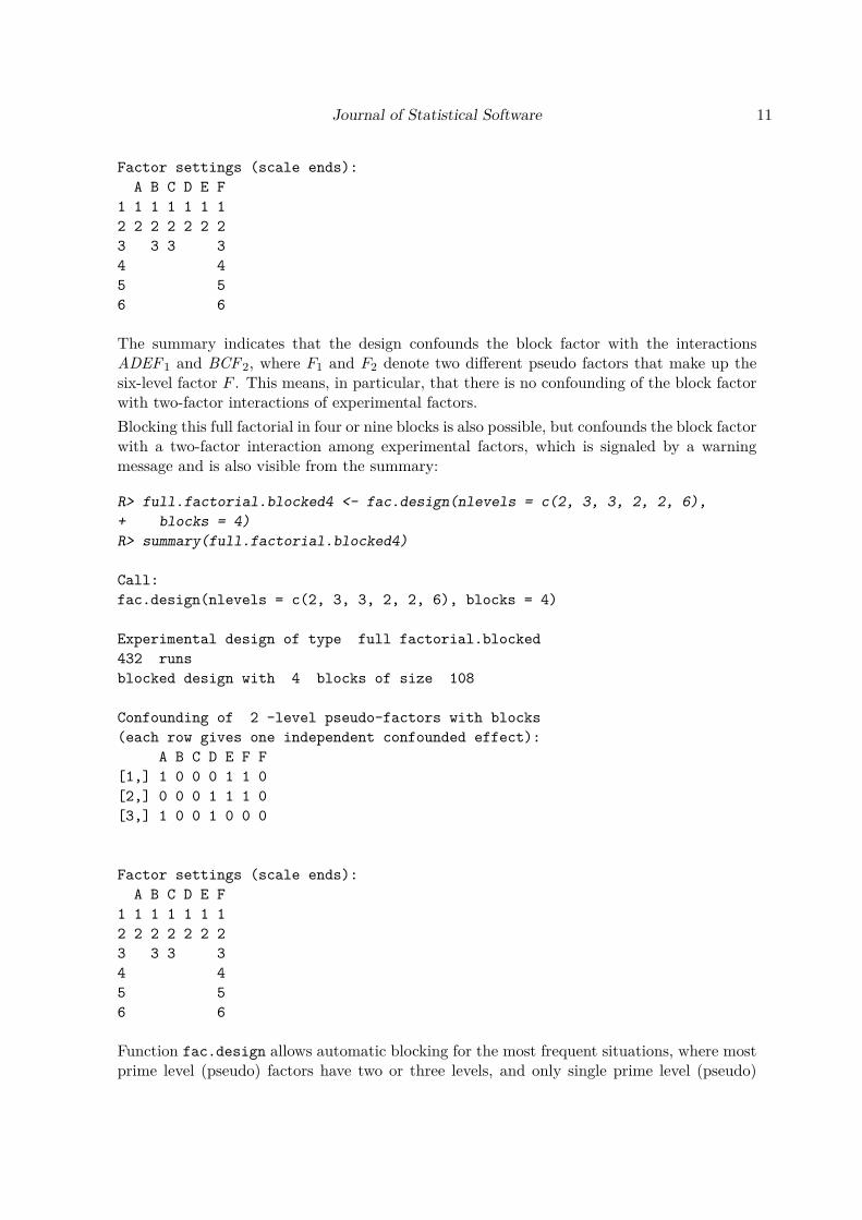
The summary indicates that the design confounds the block factor with the interactionsADEF1 and BCF2, where F1 and F2 denote two different pseudo factors that make up thesix-level factor F . This means, in particular, that there is no confounding of the block factorwith two-factor interactions of experimental factors.Blocking this full factorial in four or nine blocks is also possible, but confounds the block factorwith a two-factor interaction among experimental factors, which is signaled by a warningmessage and is also visible from the summary:
R> full.factorial.blocked4 <- fac.design(nlevels = c(2, 3, 3, 2, 2, 6),+ blocks = 4)R> summary(full.factorial.blocked4)
Call:fac.design(nlevels = c(2, 3, 3, 2, 2, 6), blocks = 4)
Experimental design of type full factorial.blocked432 runsblocked design with 4 blocks of size 108
Confounding of 2 -level pseudo-factors with blocks(each row gives one independent confounded effect):
A B C D E F F[1,] 1 0 0 0 1 1 0[2,] 0 0 0 1 1 1 0[3,] 1 0 0 1 0 0 0
Factor settings (scale ends):A B C D E F
1 1 1 1 1 1 12 2 2 2 2 2 23 3 3 34 45 56 6
Function fac.design allows automatic blocking for the most frequent situations, where mostprime level (pseudo) factors have two or three levels, and only single prime level (pseudo)

12 DoE.base for Factorial Experiments in R
factors have more than three levels; there is also a limit on the number of 2- and 3-level factors(see the package manual).We now consider an example, for which block generators have to be manually specified: Forblocking a full factorial in one 2-level factor, three 5-level factors and one 10-level factor into25 blocks, the prime 5 is needed twice for creating the block factor; thus, two block generatorsfor the prime 5 need to be specified. These can be given as a matrix with two rows (one foreach block generator) and a column for each prime factor (in the order of factors, and withineach factor, in increasing order, i.e., 2, 5, 5, 5, 2, 5 for the present design). The followingcode yields the desired blocked full factorial for the above requirement.
R> BG <- rbind(c(0, 1, 1, 2, 0, 0), c(0, 0, 1, 1, 0, 1))R> full.factorial.blocked25 <- fac.design(nlevels = c(2, 5, 5, 5, 10),+ blocks = 25, block.gen = BG)R> summary(full.factorial.blocked25)
Call:fac.design(nlevels = c(2, 5, 5, 5, 10), blocks = 25, block.gen = BG)
Experimental design of type full factorial.blocked2500 runsblocked design with 25 blocks of size 100
Confounding of 5 -level pseudo-factors with blocks(each row gives one independent confounded effect):
A B C D E1 E2[1,] 0 1 1 2 0 0[2,] 0 0 1 1 0 1[3,] 0 1 2 3 0 1[4,] 0 1 3 4 0 2[5,] 0 1 4 0 0 3[6,] 0 1 0 1 0 4
Factor settings (scale ends):A B C D E
1 1 1 1 1 12 2 2 2 2 23 3 3 3 34 4 4 4 45 5 5 5 56 67 78 89 910 10
The above design is reasonable and does not confound two-factor interactions of experimental

Journal of Statistical Software 13
factors with the block factor. Function fac.design would throw an error, if the chosen blockgenerator confounded a block effect with a main effect contrast of experimental factors or didnot provide an appropriate number of blocks. Apart from these gross issues, responsibilityfor an appropriate choice of block.gen is completely with the user.If the user is not able to come up with a satisfactory block structure, function regular.designfrom package planor can be used to create a design with the required properties (see codebelow). If that function takes a very long time for a reasonably-sized problem, there is inmany cases no solution for the requested situation; it can, however, also mean that an existingsolution is difficult to find for regular designs with factors that have non-prime numbers oflevels.
R> library("planor")R> planor.blocked25 <- regular.design(+ factors = c("Block", "A", "B", "C", "D", "E"),+ nlevels = c(25, 2, 5, 5, 5, 10), block = ~Block, nunits = 2500,+ model = ~ (A + B + C + D + E) ^ 2 + Block,+ estimate = ~ (A + B + C + D + E) ^ 2)
The search is closed: max.sol = 1 solution(s) foundThe search is closed: max.sol = 1 solution(s) found
For the design planor.blocked25, the estimate option guarantees that blocks are not con-founded with two-factor interactions. The block generator used by function regular.designis different from the one chosen in function fac.design above, but of the same quality withrespect to the GMA criterion. This can be verified by applying function GWLP or functionlengths to both designs (as mentioned before, lengths is faster for designs with many runs):
R> round(lengths(full.factorial.blocked25, with.blocks = TRUE), 2)
2 3 4 50 0 16 8
R> round(lengths(data2design(getDesign(planor.blocked25))), 2)
2 3 4 50 0 16 8
Neither function fac.design nor function regular.design from package planor guaranteesoptimality of the confounding structure, and neither is generally superior to the other.
5. Orthogonal arrays with package DoE.baseIf more than two levels are required for some factors, but a full factorial cannot be afforded, aregular or non-regular orthogonal array can be used. For the creation of regular designs, alsowith mixed levels, function regular.design from package planor is very useful. As seen inthe code of the previous section, the function can specify a model and separately a (sub)model

14 DoE.base for Factorial Experiments in R
to be estimable; in this way, it was, e.g., possible to treat the block factor differently fromthe other factors. Note, however, that it is not possible to generate non-regular designs, andthat no effort is made at a better design in terms of overall model robustness, whenever therequested estimability requirements are satisfied. Furthermore, creation of some designs takesa very long time, even for relatively small designs (e.g., 32 runs).Package DoE.base pursues a different route: It contains the previously-mentioned catalog oforthogonal arrays; most of its arrays have been taken from Kuhfeld (2010). In addition, sinceversion 0.28, it contains a small separate catalog oacat3 of orthogonal arrays of strengthat least 3 from other sources. Similarly to most experimental design software, the defaultapproach of function oa.design is to use the smallest array possible and to take columnswith the requested numbers of levels from left to right until the design has been filled. If theuser does not influence the chosen columns with the columns option, a warning is issued tomake the user aware of potential improvements. The following subsections discuss the catalogsoacat and oacat3 and ways to select arrays from them, the optimization of column selectionfrom a selected array, and ways to inspect experimental plans regarding their suitability forthe experiment at hand.
5.1. The data frames oacat and oacat3 and the function show.oas
The arrays available in package DoE.base are documented in the data frames oacat andoacat3; oacat contains strength 2 arrays, oacat3 a selection of stronger arrays. Both dataframes contain the following columns:
• name gives a structured array name, which indicates the number of runs and the fre-quency of factors with different numbers of levels; for example, the name L18.2.1.3.7indicates 18 runs with one 2-level factor and seven 3-level factors. nruns directly givesthe number of runs. n2 to n72 give the number of factors with 2 to 72 levels. Thus, forL18.2.1.3.7, nruns = 18, n2 = 1, n3 = 7, and all other nx entries have the value 0.
• lineage contains a string variable which indicates how the array was constructed fromso-called parent arrays. An empty string indicates that the array itself is a parent array.Parent arrays are stored in the package and are objects of class ‘oa’, which are matricesthat usually contain an "origin" attribute and sometimes also a "comment" attribute.Arrays with a lineage entry are constructed from the parent arrays.
• Logical columns indicate a full factorial array (ff), an array that is R2 regular accordingto the definition by Grömping and Bailey (2016) (regular.strict with only averageR2 values 0 and 1 for all factor sets), or an array that is CC regular according to thedefinition by Grömping and Bailey (2016), if their conjecture holds, i.e., if it suffices tocheck for squared canonical correlations 0 and 1 for all full resolution factor sets only(regular); for some large arrays, the necessary checks for CC regularity – even giventhe conjecture – have not been fully done, so that it is conceivable (but considered highlyunlikely) that some of the designs indicated as regular may be non-regular according toa higher order non-regularity.
• Column SCones contains the number of squared canonical correlations in R factor setsthat are one.
• Columns GR and GRind contain the GR and GRind values, respectively.

Journal of Statistical Software 15
• Columns maxAR and maxSC contain the maximum average R2 or squared canonical cor-relation, respectively.
• Column dfe provides the number of error degrees of freedom, if all columns of the arrayare used.
• Columns A3 to A8 provide the numbers of generalized words of lengths 3 to 8. (Thereare no words of shorter lengths, of course.)
It is possible to use the data frames oacat or oacat3 directly for inspecting which arraysof a certain nature are available, for example for finding strength 2 32-run arrays which areregular but not strictly regular:
R> oacat$name[oacat$nruns == 32 & oacat$regular & !oacat$regular.strict]
[1] "L32.2.28.4.1" "L32.2.25.4.2" "L32.2.24.8.1"[4] "L32.2.22.4.3" "L32.2.21.4.1.8.1" "L32.2.19.4.4"[7] "L32.2.18.4.2.8.1" "L32.2.16.4.5" "L32.2.16.16.1"
[10] "L32.2.15.4.3.8.1" "L32.2.13.4.6" "L32.2.12.4.4.8.1"[13] "L32.2.10.4.7" "L32.2.9.4.5.8.1" "L32.2.7.4.8"[16] "L32.2.6.4.6.8.1" "L32.2.4.4.9" "L32.2.3.4.7.8.1"[19] "L32.4.8.8.1"
The author prefers non-regular arrays for many situations, at least for the creation of screeningdesigns. Looking at regular arrays in package DoE.base may nevertheless be of interest, iffunction regular.design of package planor runs for a long time without indicating failure fora run size that is in the scope of package DoE.base: If there is a regular array of the desiredsize in DoE.base, this array can be inspected and perhaps used after column optimization(see Section 5.2). Also, in principle, function regular.design can be expected to eventuallysucceed, unless estimability requirements make the existing array unsuitable.The function show.oas allows inspection of the available arrays in a more convenient way; itshows arrays from oacat, unless option Rgt3 = TRUE requests arrays from oacat3. Suppose,for example, that a design for three 2-level factors, two 3-level factors and one 6-level factoris to be created, and between 20 and 54 runs are affordable (a full factorial would have 432).The following statement allows to inspect the candidate arrays, displaying also the qualitymetrics:
R> show.oas(nruns = c(20, 54), nlevels = c(2, 3, 3, 2, 2, 6),+ showmetrics = TRUE)
5 arrays foundname nruns lineage GR GRind regular SCones A3 A4
78 L36.2.13.3.2.6.1 36 3.00 3.00 FALSE 6 45.3 158.481 L36.2.10.3.8.6.1 36 3.18 3.18 FALSE 0 130.3 737.283 L36.2.9.3.4.6.2 36 3.00 3.00 FALSE 17 82.3 338.287 L36.2.3.3.9.6.1 36 3.18 3.00 FALSE 12 73.8 300.288 L36.2.3.3.2.6.3 36 3.00 3.00 FALSE 37 35.6 73.1

16 DoE.base for Factorial Experiments in R
A5 A6 A7 A878 426 1010 1753.2 2306.881 3063 11096 31380.8 68828.183 1025 2828 5507.5 7780.087 912 2404 4354.2 5793.488 120 125 63.5 13.9
Only arrays in 36 runs have been found; these are quite different in the available patternsof numbers of levels, and therefore the quality metrics (especially the Ak) are not directlycomparable. Nevertheless, the values for GR and GRind suggest that one might try thearray L36.2.10.3.8.6.1, which is the only one without any completely confounded degreeof freedom.
5.2. Optimization methods for function oa.design
Function oa.design allows to select an array, and to specify columns from that array eithermanually or by an optimization approach. As was mentioned earlier, if no array is specified,the function picks the first (and thus smallest) array in the catalog that is able to accommodatethe requested factors. If no column selection approach is specified, the function simply takesthe first available columns (from left to right).The code below compares three designs:
• an unoptimized default design (i.e., the left-most suitable columns of the first arrayencountered, which is the L36.2.13.3.2.6.1);
• an optimized default design with optimization option columns = "min34" (i.e., an op-timized choice of columns from the array L36.2.13.3.2.6.1, optimization being withrespect to the number of generalized words of length 3, and subsequently length 4);
• and an optimized design obtained by selecting columns from the array L36.2.10.3.8.6.1selected in Section 5.1 because of its GRind value.
R> oa.default <- oa.design(nlevels = c(2, 3, 3, 2, 2, 6))R> GWLP(oa.default, digits = 2)
0 1 2 3 4 5 61.00 0.00 0.00 5.78 2.11 2.44 0.67
R> oa.optimized <- oa.design(nlevels = c(2, 3, 3, 2, 2, 6),+ columns = "min34")R> GWLP(oa.optimized, digits = 2)
0 1 2 3 4 5 61.00 0.00 0.00 4.11 3.61 2.78 0.50
R> oa.manualoptimized <- oa.design(L36.2.10.3.8.6.1,+ nlevels = c(2, 3, 3, 2, 2, 6), columns = "min34")R> GWLP(oa.manualoptimized, digits = 2)

Journal of Statistical Software 17
0 1 2 3 4 5 61.00 0.00 0.00 2.44 6.44 1.78 0.33
Clearly, optimization improves the design from the default array, and the optimized pre-selected array is even better.There are various methods for optimizing column allocation (see the documentation of func-tion oa.design in the manual); columns = "min34" is the most important one among these.Depending on the number of columns on offer and the number of columns to be selected, op-timization can take a very long time; in the above examples,
(133)·(2
2)
= 286 or(10
3)·(8
2)
= 3360column choices had to be checked, which is doable in reasonably short time. For larger de-signs, the resource implications of the numbers of available columns of the required lengthsmay also be considered in selecting an array to use.
5.3. Blocking general orthogonal arrays
Suppose a design with the above factors is to be run, and the 6-level factor is a blockingfactor. In that case, the design should be randomized such that runs are randomized withinblocks. Function oa.design does not directly allow to block randomization. However, thefunction rerandomize.design allows a post-hoc randomization within a single design factordeclared as the block factor.
R> blockedoa1 <- rerandomize.design(oa.manualoptimized, seed = 24652,+ block = "F")R> blockedoa1
run.no run.no.std.rp F A B C D E1 1 22.5.4 5 2 1 1 1 22 2 5.5.2 5 1 2 3 2 23 3 15.5.3 5 1 3 3 1 14 4 1.5.1 5 1 1 2 1 15 5 35.5.6 5 2 2 1 2 16 6 33.5.5 5 2 3 2 2 2
run.no run.no.std.rp F A B C D E7 7 32.3.5 3 2 2 1 2 28 8 14.3.3 3 1 2 2 1 19 9 34.3.6 3 2 1 3 2 110 10 4.3.2 3 1 1 2 2 211 11 3.3.1 3 1 3 1 1 112 12 24.3.4 3 2 3 3 1 2
run.no run.no.std.rp F A B C D E13 13 18.4.3 4 1 3 3 2 214 14 26.4.5 4 2 2 2 2 115 15 30.4.6 4 2 3 1 1 116 16 11.4.2 4 1 2 1 1 217 17 7.4.1 4 1 1 3 2 118 18 19.4.4 4 2 1 2 1 2
run.no run.no.std.rp F A B C D E

18 DoE.base for Factorial Experiments in R
19 19 10.2.2 2 1 1 3 1 220 20 21.2.4 2 2 3 1 1 221 21 29.2.6 2 2 2 3 1 122 22 17.2.3 2 1 2 2 2 223 23 9.2.1 2 1 3 2 2 124 24 25.2.5 2 2 1 1 2 1
run.no run.no.std.rp F A B C D E25 25 20.6.4 6 2 2 3 1 226 26 16.6.3 6 1 1 1 2 227 27 8.6.1 6 1 2 1 2 128 28 12.6.2 6 1 3 2 1 229 29 28.6.6 6 2 1 2 1 130 30 27.6.5 6 2 3 3 2 1
run.no run.no.std.rp F A B C D E31 31 31.1.5 1 2 1 3 2 232 32 36.1.6 1 2 3 2 2 133 33 13.1.3 1 1 1 1 1 134 34 2.1.1 1 1 2 3 1 135 35 23.1.4 1 2 2 2 1 236 36 6.1.2 1 1 3 1 2 2class=design, type= oa.blockedNOTE: columns run.no and run.no.std.rp are annotation,not part of the data frame
Function GWLP per default ignores confounding with the block factor, but can be requestedto include it using the with.block = TRUE option:
R> GWLP(blockedoa1, digits = 2)
0 1 2 3 4 51.00 0.00 0.00 0.28 0.33 0.39
R> GWLP(blockedoa1, with.block = TRUE, digits = 2)
0 1 2 3 4 51.00 0.00 0.00 2.44 6.44 1.78
For designs that can also be created with function FrF2 (package FrF2) and/or functionregular.design (package planor), using one of the latter two may be a better choice, sincethey allow a more direct control over design quality via minimum aberration or estimableeffects: The code below (results not shown) creates and inspects a 16-run design with eight2-level factors in eight blocks of size 2 with all three methods; in all three cases, the design isresolution IV in terms of the experimental factors, which is systematically requested in bothFrF2 (by the minimum aberration approach of the function) and regular.design (by themodel and estimate options). For function oa.design, the design quality is not as finelytunable, apart from the overall optimization that may precede usage of an array for whichnot all columns are used. For the designs below, however, the quality is the same for all three

Journal of Statistical Software 19
designs: The GWLPs, starting with A3, are (28, 14, 56, 0, 28, 1) including the block factorand (0, 14, 0, 0, 0, 1) for the experimental factors alone.
R> planFrF2 <- FrF2(16, 8, blocks = 8, alias.block.2fis = TRUE)R> planDoEbase <- oa.design(L16.2.8.8.1,+ nlevels = c(2, 2, 2, 2, 2, 2, 2, 2, 8),+ factor.names = c(Letters[1:8], "Block"))R> planDoEbase <- rerandomize.design(planDoEbase, seed = 31525,+ block = "Block")R> planplanor <- regular.design(factors = c(Letters[1:8], "Block"),+ nlevels = c(rep(2, 8), 8),+ model = ~ (A + B + C + D + E + F + G + H) ^ 2 + Block,+ estimate = ~ A + B + C + D + E + F + G + H,+ nunits = 16, randomize = ~ Block / UNITS)R> GWLP(planFrF2, with.block = TRUE)R> GWLP(planFrF2)R> GWLP(planDoEbase, with.block = TRUE)R> GWLP(planDoEbase)R> GWLP(planplanor@design)R> GWLP(planplanor@design[, 1:8])
5.4. Inspection methods for factorial designs
Any experimental plan should be carefully checked before using it for experimentation, sinceexperimentation usually involves a lot of effort: Adverse consequences from mistakes in designcreation may be severe, but can often be prevented without much trouble, if attended to atthe design creation stage. For example, when implementing a self-chosen blocking, mistakescan easily happen:
R> planstupid <- FrF2(16, 8, blocks = c("AB", "AC", "BCD"),+ alias.block.2fis = TRUE)R> GWLP(planstupid, with.blocks = TRUE)R> plot(data2design(undesign(planstupid)), select = "all2")
A simple check of the GWLP can serve as a first indication whether the design behavesas expected; here we find A2 = 4 (not shown), which is of course undesirable. Furtherchecks can involve plotting. The plot command in the code above reveals (not shown) thatfactors D, F , G and H are aliased with the block factor for the design planstupid, whichexplains the four words of length 2. Instead of looking at all two-factor sets with optionselect = "all2", one can also look at a percentage of worst cases (see below). Note thatthe data2design(undesign()) construction is used for incorporating the block factor, sincethe plot method for class ‘design’ does not have a with.blocks option and works on thedesign factors only.We now visualize the worst case confounding of the two optimized designs discussed in Sec-tion 5.2:
R> plot(oa.optimized, select = "worst", selprop = 0.05)

20 DoE.base for Factorial Experiments in R
●●●●
●●●●
●●
●●
●●●●
●●
●●
●●●●
●●
●●
●●●●
●●●●
C
B F
3
65
4321
2
6543
21
1
1 2 3
654
321
(a) Autoselected array, worstcase.
●●
●●
●●
●●
●●
●●
●●
●●
●●
C
B F
3
65
43
21
2
65
432
1
1
1 2 3
654
32
1
(b) Manually selected array,same case.
●
●
●
●
●
●
●
●
●●
●●
C
A F
2
654
32
1
1
1 2 3
65
43
21
(c) Manually selected array,worst case.
Figure 2: Mosaic plots of triples of factors.
R> plot(oa.manualoptimized, select = c(2, 3, 6))R> plot(oa.manualoptimized, select = "worst", selprop = 0.05)
The code above generates the three mosaic plots of Figure 2. The optimized design basedon the array that was automatically picked severely confounds the interaction of the two3-level factors with the 6-level factor (factors 2, 3 and 6 of the design): A mosaic plot ofthat projection is created by the first line of the above code and is shown in Figure 2(a). Itshows that the interaction of the two 3-level factors restricts the 6-level factor to a third ofits possibilities only, which is the most severe form of aliasing possible for a triple of factorswith this level combination; of the 54 possible level combinations in this triple of factors,the design contains 18 distinct variants only (instead of the possible 36). In comparison, amosaic plot of the same projection for the optimized manually selected design shows a muchbetter picture: Now, the design has 36 distinct level combinations, the maximum possible(see Figure 2(b)). The worst case confounding for that design is shown in Figure 2(c). It isdistinctly less severe than that of Figure 2(a); however, apart from the one worst case shownin Figure 2(a), the optimized automatically-selected design is also quite reasonable.Mosaic plots concentrate on individual low order projections. Package DoE.base offers anotherdiagnostic plot for looking at the entire design at once: Function corrPlot inspects thecorrelations between model matrix columns. The creation of function corrPlot was inspiredby function colormap of package daewr (Lawson 2016). Figure 4 in Section 6.1 illustratesits default version applied to a real life example. This function also offers a possibility toinclude the design’s run order among the effects to be considered, since there are applicationsfor which the run order might be of relevance. For such situations, a simple approach couldbe to re-randomize the design (with function rerandomize.design) until a randomization isencountered for which the correlation of the run order to relevant effect columns (as shownin the plot of absolute correlations) is reasonably small.Numeric quality criteria can also be obtained; the function names for obtaining them werealready mentioned in Section 3.2. These advanced criteria might deter practitioners but maybe useful for experts: The function GRind calculates the metrics introduced by Grömping andXu (2014) with the additional detail proposed in Grömping (2017a). For example, the codebelow shows that the optimized design based on the manually selected array has a clearly

Journal of Statistical Software 21
better overall behavior regarding factor-specific worst case confounding (GRtot,i and GRind,i;see Section 3.2) than the optimized design based on the automatically selected first array.
R> GRind1 <- GRind(oa.optimized)R> GRind2 <- GRind(oa.manualoptimized)R> print(cbind(rep(c("oa.optimized", "oa.manualoptimized"), each = 2),+ rbind(GRind1$GR.i, GRind2$GR.i)), quote = FALSE)
A B C D E FGRtot.i oa.optimized 3.667 3 3 3.423 3.423 3.368GRind.i oa.optimized 3.667 3 3 3.423 3.423 3GRtot.i oa.manualoptimized 3.184 3.5 3.423 3.423 3.667 3.635GRind.i oa.manualoptimized 3.184 3.5 3.423 3.423 3.667 3.423
6. An example from plant biotechnologyVasilev et al. (2014) investigated cultivation factors for geraniol production by plant cells.There were four quantitative 2-level factors, two 3-level factors (one quantitative and onequalitative) and one qualitative 4-level factor. The data, including response values, havebeen published with the paper and are also included in package DoE.base as object VSGFS.The 2-level factors are coded in −1/+1 coding, the other factors in R’s default dummy coding.
6.1. Creating and inspecting the design
For this experiment, a full factorial design would have had 576 runs. It would certainly havebeen necessary to conduct it in blocks, say in eight blocks of size 72 each. Such a designcould have been created by function fac.design or by function regular.design of packageplanor, as shown in Section 4.A full factorial design appeared neither feasible nor appropriate for the screening situation ofthe experiment. Instead, the design was conducted using a 72-run orthogonal array, whichwas generated with function oa.design, using automatic optimization (option columns ="min34") of the manually pre-selected array L72.2.43.3.8.4.1.6.1. The optimization tookquite a long time and resulted in the selection of columns 4, 22, 37, 41 for the 2-level factors,46 and 48 for the 3-level factors, and 52 for the 4-level factor. The design is available as objectVSGFS, and the code for reproducing it can be found in the manual.When constructing the experimental plan for VSGFS, the array was pre-selected by intuitionand trial and error from all 33 72-run designs that can accommodate the requested fac-tors, using the versions of function show.oas and data frame oacat available at the time(no metrics information was contained in oacat, and thus, metric-based filtering was notpossible with function show.oas). A key driver for the ad-hoc selection of designs withinwhich to select columns was the number of choices a design offered for accommodating thefactors; this criterion was used intuitively rather than systematically; post-hoc, note thatthe actually chosen design offers 3455480 choices, ranking fourth behind three designs of-fering 8959566, 5151510 and 3455760 possibilities. After the resource-intensive optimizationof the L72.2.43.3.8.4.1.6.1, some further designs with distinctly fewer possibilities wereadditionally tried; all of these yielded worse A3.

22 DoE.base for Factorial Experiments in R
With the present possibilities of function show.oas, the GRgt3 = "ind" option (i.e., request-ing that GRind > 3 which means absence of any instance of complete confounding for indi-vidual degrees of freedom), one can pick arrays that are particularly promising for screeningpurposes. The following command shows the available arrays without any complete con-founding for the example situation, together with the GR metrics (requested by the showGRsoption):
R> show.oas(nlevels = c(2, 2, 2, 3, 2, 3, 4), GRgt3 = "ind", showGRs = TRUE)
4 arrays foundname nruns lineage GR
366 L72.2.53.3.2.4.1 72 3.18380 L72.2.44.3.12.4.1 72 3.18382 L72.2.43.3.8.4.1.6.1 72 3.18431 L72.2.13.3.25.4.1 72 3~24;24~1;:(24~1!2~13;3~1;4~1;) 3.18
GRind366 3.18380 3.18382 3.18431 3.13
The array used in actual experimentation is the third array in this list; thus, the intuitiveapproach was lucky to pick a particularly promising array in this case. It can be expected thatall four arrays listed above are reasonably suited for screening the experimental factors. Asthe designs are far from saturated, optimal column allocation can substantially improve theworst case confounding (and thus GR and GRind): For the eventual design, the output belowshows GR = GRind = 3.6; ARFT and SCFT have been suppressed, because their backgroundis outside the scope of this paper.
R> GRind(VSGFS, arft = FALSE, scft = FALSE)
$GRsGR GRind
3.667 3.667
$GR.iLight ShakFreq InocSize FilledVol CM Sugar CDs
GRtot.i 3.667 3.667 3.667 3.864 3.667 3.864 3.808GRind.i 3.667 3.667 3.667 3.808 3.667 3.808 3.667
attr(,"class")[1] "GRind" "list"
For illustrating the worst case degree of confounding, Figure 3 shows the triple 3, 5, 7 in quitereasonable balance (this is one of the two worst case triples); the option sub = "A" in the coderequests that the A3 value for the triple is printed as a subtitle. Figure 4 shows for the entiredesign that the main effect model matrix columns have reasonably low correlations with

Journal of Statistical Software 23
R> plot(VSGFS, select = list(c(3, 5, 7)), sub = "A")
A3 = 0.1111
CM
Inoc
Siz
e
CD
s
IS+
CD
4C
D3
CD
2C
D1
IS−
CM− CM+
CD
4C
D3
CD
2C
D1
Figure 3: Mosaic plot for the worst case triple in the VSGFS example.
R> corrPlot(VSGFS)
Plot of absolute correlations
CDs3CDs2CDs1
Sugar2Sugar1
CM1FilledVol2FilledVol1InocSize1
ShakFreq1Light1
Ligh
t1:S
hakF
req1
Ligh
t1:In
ocS
ize1
Ligh
t1:F
illed
Vol
1Li
ght1
:Fill
edV
ol2
Ligh
t1:C
M1
Ligh
t1:S
ugar
1Li
ght1
:Sug
ar2
Ligh
t1:C
Ds1
Ligh
t1:C
Ds2
Ligh
t1:C
Ds3
Sha
kFre
q1:In
ocS
ize1
Sha
kFre
q1:F
illed
Vol
1S
hakF
req1
:Fill
edV
ol2
Sha
kFre
q1:C
M1
Sha
kFre
q1:S
ugar
1S
hakF
req1
:Sug
ar2
Sha
kFre
q1:C
Ds1
Sha
kFre
q1:C
Ds2
Sha
kFre
q1:C
Ds3
Inoc
Siz
e1:F
illed
Vol
1In
ocS
ize1
:Fill
edV
ol2
Inoc
Siz
e1:C
M1
Inoc
Siz
e1:S
ugar
1In
ocS
ize1
:Sug
ar2
Inoc
Siz
e1:C
Ds1
Inoc
Siz
e1:C
Ds2
Inoc
Siz
e1:C
Ds3
Fill
edV
ol1:
CM
1F
illed
Vol
2:C
M1
Fill
edV
ol1:
Sug
ar1
Fill
edV
ol2:
Sug
ar1
Fill
edV
ol1:
Sug
ar2
Fill
edV
ol2:
Sug
ar2
Fill
edV
ol1:
CD
s1F
illed
Vol
2:C
Ds1
Fill
edV
ol1:
CD
s2F
illed
Vol
2:C
Ds2
Fill
edV
ol1:
CD
s3F
illed
Vol
2:C
Ds3
CM
1:S
ugar
1C
M1:
Sug
ar2
CM
1:C
Ds1
CM
1:C
Ds2
CM
1:C
Ds3
Sug
ar1:
CD
s1S
ugar
2:C
Ds1
Sug
ar1:
CD
s2S
ugar
2:C
Ds2
Sug
ar1:
CD
s3S
ugar
2:C
Ds3
0.00
0.05
0.10
0.15
0.20
0.25
Figure 4: Plot of absolute correlations of main effects model matrix columns with two factorinteraction model matrix columns for the VSGFS example (default normalized orthogonalcoding is the Xu Wu coding).
the two-factor interaction model matrix columns; note that function corrPlot defaults torecoding all factors in normalized orthogonal coding (see also Section 7), in order to eliminateavoidable confounding.The team was happy with the design and used it for collecting the data. Software-wise,data collection happened in Excel, exporting the randomized design with the export.design

24 DoE.base for Factorial Experiments in R
function and re-importing it after data entry using the exported RDA file together with aCSV file with response values added to the data rows using function add.response.
6.2. Analyzing experimental data
The data frame VSGFS contains the experiment with response data. Package DoE.base offersa few functions for analysis purposes:
• The plot method for class ‘design’, in case of data with responses, creates simple maineffects plots, by invoking the plot method from package graphics.
• The lm method for class ‘design’ runs a linear model with a modifiable default degree.For orthogonal arrays created with function oa.design, the default degree is one, i.e.,a model with main effects only. Linear models can of course also be run by the lmfunction from the core package stats, and analysis of variance functionality can also beused (see below).
• The halfnormal method for classes ‘lm’ or ‘design’ creates a half-normal effects plot(see Section 7).
Of course, in general, other R functionality can also be used, for example interaction plotsor functionality for mixed model analysis (not applicable for the example data). The func-tionality for handling repeated measurement data or replicated data (also not needed for thisexample) has been described for package FrF2 in Sections 5.3 and 5.9 of Grömping (2014c)and is analogous here.Main effects plots can be obtained by the simple command plot(VSGFS), which creates theseplots for all three response variables. Figure 5 shows the plots with default labeling, arrangedwith three plots on one page and reduced margin sizes. Of course, one would usually adaptthe annotation for final reports or publications. The plot shows that the sugar sucrose is verybeneficial for the biomass, not very good for the content, but nevertheless, because of thestrong effect on biomass, beneficial for the yield. The content apparently can be increased bychoosing the sugar mannitol, level one of factor CD and the +-level of light. Apart from the+-level of light, the other settings for high content are not helpful for overall yield.An assessment of significance can be obtained from a linear model analysis. This can beobtained separately for each response, for example for the content. Here, the analysis confirmsthe findings from the main effects plot.
R> summary(lm(VSGFS, response = "Content"))
Number of observations used: 72Formula:Content ~ Light + ShakFreq + InocSize + FilledVol + CM + Sugar +
CDs
Call:lm.default(formula = fo, data = model.frame(fo, data = formula))
Residuals:

Journal of Statistical Software 25
23
45
Factors
mea
n of
Bio
mas
s
Lght−
Lght+
SF−SF+
IS−
IS+
FV−
FV0
FV+
CM−CM+
Suc
Gluc
Mannit
CD1
CD2CD3CD4
Light ShakFreq InocSize FilledVol CM Sugar CDs
17.5
18.0
18.5
19.0
19.5
20.0
Factors
mea
n of
Con
tent
Lght−
Lght+
SF−
SF+IS−IS+
FV−
FV0
FV+
CM−
CM+
Suc
Gluc
Mannit
CD1
CD2CD3
CD4
Light ShakFreq InocSize FilledVol CM Sugar CDs
3040
5060
7080
9010
0
mea
n of
Yie
ld
Lght−
Lght+
SF−SF+
IS−
IS+
FV−
FV0
FV+
CM−CM+
Suc
Gluc
Mannit
CD1
CD2CD3CD4
Light ShakFreq InocSize FilledVol CM Sugar CDs
Figure 5: Main effects plots for all three responses.

26 DoE.base for Factorial Experiments in R
Min 1Q Median 3Q Max-2.5472 -1.1746 -0.1052 0.7008 4.6994
Coefficients:Estimate Std. Error t value Pr(>|t|)
(Intercept) 18.67611 0.55106 33.891 < 2e-16 ***Light1 0.63264 0.19483 3.247 0.00191 **ShakFreq1 -0.15792 0.19483 -0.811 0.42083InocSize1 0.05903 0.19483 0.303 0.76296FilledVolFV0 -0.36958 0.47723 -0.774 0.44172FilledVolFV+ -0.14958 0.47723 -0.313 0.75503CM1 -0.22069 0.19483 -1.133 0.26182SugarGluc 0.54917 0.47723 1.151 0.25441SugarMannit 2.51167 0.47723 5.263 2e-06 ***CDsCD2 -1.63222 0.55106 -2.962 0.00438 **CDsCD3 -1.57111 0.55106 -2.851 0.00597 **CDsCD4 -1.10722 0.55106 -2.009 0.04901 *---Signif. codes: 0 '***' 0.001 '**' 0.01 '*' 0.05 '.' 0.1 ' ' 1
Residual standard error: 1.653 on 60 degrees of freedomMultiple R-squared: 0.4787, Adjusted R-squared: 0.3831F-statistic: 5.008 on 11 and 60 DF, p-value: 1.75e-05
The model explains less than 50% of the response variability, which is far from perfect; therelatively large unexplained variation can be due both to random error and to the presenceof interaction effects not captured in the main effects model. Nevertheless, the main effectsresults are trustworthy. The strong heredity principle – interactions are only active if boththeir component factors are active – suggests to look at a model with the three active maineffect factors and their interactions, which leaves a somewhat confusing picture (not shown).For the data at hand, there are enough degrees of freedom to run an Anova analysis with thefull degree 2 model. Of course, while main effects are orthogonal to each other, two-factorinteractions can be slightly confounded with main effects and severely confounded with othertwo-factor interactions. However, at least, the theory tells us that the estimable effects canbe estimated without bias (unless effects of order higher than two bias them). As Anovaanalyses sums of squares, the analysis is invariant with respect to factor coding. In orderto obtain an order-invariant assessment of significance, the function Anova from package car(Fox and Weisberg 2011) can be used; contrary to function anova from package stats, Anovaavoids order-dependence by using type II sums of squares, which condition on all other effectsexcept for the ones that contain the effect under investigation. The results point to the maineffects that were also identified before, and a liberal look at p values additionally indicatessome marginal two-factor interactions (sugar with each of InocSize, FilledVol, CDs, Light,and ShakFreq:CM, which is completely unrelated to the active main effects).
R> library("car")R> Anova(lm(VSGFS, response = "Content", degree = 2))

Journal of Statistical Software 27
Anova Table (Type II tests)
Response: ContentSum Sq Df F value Pr(>F)
Light 16.345 1 8.2606 0.0165515 *ShakFreq 0.483 1 0.2441 0.6319195InocSize 1.604 1 0.8105 0.3891387FilledVol 0.889 2 0.2247 0.8026463CM 0.805 1 0.4069 0.5378565Sugar 67.692 2 17.1048 0.0005921 ***CDs 29.468 3 4.9642 0.0230814 *Light:ShakFreq 1.672 1 0.8450 0.3795988Light:InocSize 0.320 1 0.1616 0.6961803Light:FilledVol 3.296 2 0.8330 0.4628103Light:CM 2.874 1 1.4524 0.2558948Light:Sugar 11.387 2 2.8774 0.1030201Light:CDs 6.073 3 1.0231 0.4231004ShakFreq:InocSize 1.162 1 0.5871 0.4612301ShakFreq:FilledVol 0.420 2 0.1061 0.9003686ShakFreq:CM 6.303 1 3.1856 0.1046054ShakFreq:Sugar 3.074 2 0.7767 0.4857813ShakFreq:CDs 11.717 3 1.9738 0.1819413InocSize:FilledVol 1.626 2 0.4109 0.6737704InocSize:CM 0.752 1 0.3802 0.5512885InocSize:Sugar 20.475 2 5.1739 0.0286697 *InocSize:CDs 7.710 3 1.2989 0.3280819FilledVol:CM 2.976 2 0.7521 0.4962887FilledVol:Sugar 24.172 4 3.0539 0.0692876 .FilledVol:CDs 6.333 6 0.5334 0.7719232CM:Sugar 3.387 2 0.8559 0.4538120CM:CDs 10.566 3 1.7799 0.2144014Sugar:CDs 33.075 6 2.7858 0.0734918 .Residuals 19.787 10---Signif. codes: 0 '***' 0.001 '**' 0.01 '*' 0.05 '.' 0.1 ' ' 1
Even though this design does not require analysis with half-normal effects plots, the nextsection will illustrate application of half-normal effects plots for this example.
7. Half-normal effects plotsIn (almost) saturated designs, conventional analysis of variance methods are not very suc-cessful, because there are too few degrees of freedom for error. If one assumes a screeningdesign, for which most effects are inactive, the inactive effects actually represent experimentalerror; however, it is not known a-priori, which are the active effects. Daniel (1959) proposedto use half-normal effects plots for diagnosing which effects are active, and Lenth (1989) pro-
28 DoE.base for Factorial Experiments in R
posed a numerical activity check for these, known as “Lenth’s method”. The critical valuesproposed by Lenth were later found to be conservative, and it was proposed to use simulatedones instead. Half-normal effects plots with Lenth’s method and simulated critical values areimplemented in function halfnormal of package DoE.base.
7.1. The principle
The standard use for such plots is with 2-level factors which are conventionally coded in−1/+1 coding (see, e.g., Grömping 2014c). Function halfnormal from package DoE.basecovers not only these standard situations, but also offers half-normal plots for:
• 2-level designs with a few error degrees of freedom. For these, it automatically augmentsthe estimated effects with error effects, distinguishing these into lack-of-fit and pureerror. Significance assessment can be done with Lenth’s method on the augmented setof estimates, or with other methods proposed in the literature (Larntz and Whitcomb1998; Edwards and Mee 2008). Note that error effects are not necessarily uniquelydetermined.
• 2-level designs with partially confounded effects. For these, it projects out all precedingeffects from the remaining ones (thus, the plotting points depend on the model orderfor such situations).
• Mixed level designs, for which there is no unique coding and the plotting points arecoding dependent. Mixed level designs can also have error degrees of freedom or partiallyconfounded effects.
The strategy chosen in function halfnormal seems to be similar to that applied in the JMPsoftware (SAS Institute Inc. 2018) screening platform (see Chapter 8 of SAS Institute Inc.2012), both regarding the treatment of error points and the single degree of freedom repre-sentations for factors with more than two levels. On the contrary, Design-Expert (Stat-EaseInc. 2017) does not plot individual degrees of freedom, but scaled Chi-squared values for ef-fects with more than one degree of freedom. This avoids the coding dependence, but has theadverse effect that the number of plotting points is small so that effect sparsity is not easilyachieved.The steps for augmenting the estimated effects with error degrees of freedom are described,e.g., in Grömping (2015) and are very similar also to the suggestions by Langsrud (2001) ina different context. A coarse overview works as follows:
• Make sure the model matrix X has orthogonal columns all of which have the sameEuclidean length; if this is not the case, X has to be pre-treated (see below).
• For N observations, a trivial saturated model matrix is the N -dimensional identitymatrix IN . If a distinction between lack-of-fit and pure error is sought, one can replacethis matrix by a matrix S of dummy variables for distinct runs, and additionally includeappropriately scaled orthogonal contrast matrices for replicated runs. In the following,for simplicity, IN is used.
• Residualize the matrix IN by projecting out the model matrix X, i.e., calculate theresidual matrix R = IN −X(X>X)−1X>.

Journal of Statistical Software 29
• Create the half-normal effects plot for the augmented model matrix (X|R), which hasbeen created such that it has orthogonal columns where all have the same length.
The pre-treatment mentioned in the first bullet is as follows: If X has orthogonal columnsof varying Euclidean lengths, one simply has to normalize all columns to a common length.The case of non-orthogonal columns is more demanding and will be discussed using the modelmatrix X for a full model in an unreplicated full factorial design for one 2-level and one 3-levelfactor, both in dummy coding, as given in Equation 1:
X =
Int A2 B2 B3 A2B2 A2B31 0 0 0 0 01 1 0 0 0 01 0 1 0 0 01 1 1 0 1 01 0 0 1 0 01 1 0 1 0 1
. (1)
The columns of this matrix are not orthogonal, which can be easily verified by inspectingX>X. As the intercept estimates the mean for the combination A1B1 and the coefficients forthe main effects columns estimate deviations from that level, there is an obvious dependency.With the interaction coefficients also measuring deviations of particular cells from additivity,there is another clear dependence. It is well-known which effects are estimable in factorialmodels: the overall means and the contrasts. A model matrix formulated to directly estimatethese has orthogonal columns.Xu and Wu (2001) showed that it is particularly useful to code all main effects columns usingan orthogonal coding normalized to squared length N , where N is the number of runs: Sucha coding yields orthogonal columns of the model matrix for all effects up to degree s for anyprojection of s factors from a strength s design, if the interaction columns are created inthe usual way as products of the normalized main effects contrast columns; the interactioncolumns will then also have squared Euclidean length N and will be orthogonal to eachother and to the main effects columns. Such coding will be called Xu Wu coding in thesequel. It is available in two versions in package DoE.base: There are contr.XuWu andcontr.XuWuPoly contrasts. The model matrix below is obtained by coding both factors Aand B with contr.XuWu contrasts.
X =
Int A2 B2 B3 A2B2 A2B31 −1 −
√1.5 −
√0.5
√1.5
√0.5
1 1 −√
1.5 −√
0.5 −√
1.5 −√
0.51 −1
√1.5 −
√0.5 −
√1.5
√0.5
1 1√
1.5 −√
0.5√
1.5 −√
0.51 −1 0
√2 0 −
√2
1 1 0√
2 0√
2
(2)
If the design has strength s, a model matrix in a Xu Wu coding for main effects with up tos-factor interactions can also be obtained post-hoc from a model matrix X based on non-orthogonal coding by sequential orthogonalization and normalization: Project out the firstcolumn (intercept column) from the second, which is just subtraction of the column mean.Project out the first two columns from the third and so on. In addition, one also has to

30 DoE.base for Factorial Experiments in R
normalize all columns to squared length N (or any other common Euclidean length) in orderto satisfy the requirements for a half-normal effects plot.If the model has truly confounded effects that cannot be orthogonalized by simply applyingXu Wu coding, the same orthogonalization strategy can be applied, but the consequence isnot only a recoding of in principle the same information, but an order-dependent removal ofearlier confounded effects from later confounded effects.
7.2. Example application
The example design is an orthogonal array, i.e., main effect contrasts can be estimated inde-pendently of each other. However, depending on the coding, the actual estimated coefficientsmay be correlated, as was discussed above. For example, for 2-level factors, if −1/+1 codingis used, the estimates are uncorrelated, with 0/1 (dummy) coding, however, they are cor-related. It is advisable to explicitly choose an orthogonal factor coding, ideally the Xu Wuvariant discussed above. The code below creates an orthogonal main effects model matrixwith squared Euclidean length N = 72 (output not shown).
R> VSGFS.XuWuPoly <- change.contr(VSGFS, "contr.XuWuPoly")R> round(crossprod(model.matrix(lm(VSGFS.XuWuPoly))), 2)
Per default, function halfnormal refuses to work in case of correlated main effects (exceptin case of the perfect confounding of regular designs). The option ME.partial = TRUE canbe used to change that; if the partial aliasing among main effects estimates is due to non-orthogonal coding in an orthogonal array, use of ME.partial = TRUE is acceptable in thelight of the previous considerations (see the first command to create hnauto below), althoughit seems preferable to decide on an orthogonal coding explicitly.For the example design, a main effects analysis is quite well-protected against bias fromtwo-factor interactions. However, two-factor interactions may be quite heavily confoundedwith each other. Nevertheless, we will now consider an almost saturated array in order todemonstrate the most general usage of the function halfnormal.
R> hnAuto <- halfnormal(lm(VSGFS, response = "Content", degree = 2),+ ME.partial = TRUE, cex.text = 0.9, cex = 0.9, xlim = c(0, 1.1),+ ylim = c(0, 2.8), main = "Half-normal effects plot for Content")R> hnXuWuPoly <- halfnormal(lm(VSGFS.XuWuPoly, response = "Content",+ degree = 2), cex.text = 0.9, cex = 0.9, xlim = c(0, 1.1),+ ylim = c(0, 2.8), main = "Half-normal effects plot for Content")R> hnXuWuPolyreordered <- halfnormal(lm(Content ~+ (CDs + Sugar + CM + FilledVol + InocSize + ShakFreq + Light) ^ 2,+ VSGFS.XuWuPoly), cex.text = 0.9, cex = 0.9, xlim = c(0, 1.1),+ ylim = c(0, 2.8), main = "Half-normal effects plot for Content")
Figure 6 shows half-normal effects plots from a model with all main effects and two-factorinteractions for the response variable Content. In order to demonstrate the coding dependenceof half-normal effects plots in case of factors with more than two levels, plot (a) shows theautomatic coding obtained by orthogonalizing the model matrix that results from the dummycoding of the 3- and 4-level factors in VSGFS, plot (b) contr.XuWuPoly coding. Plot (c) shows
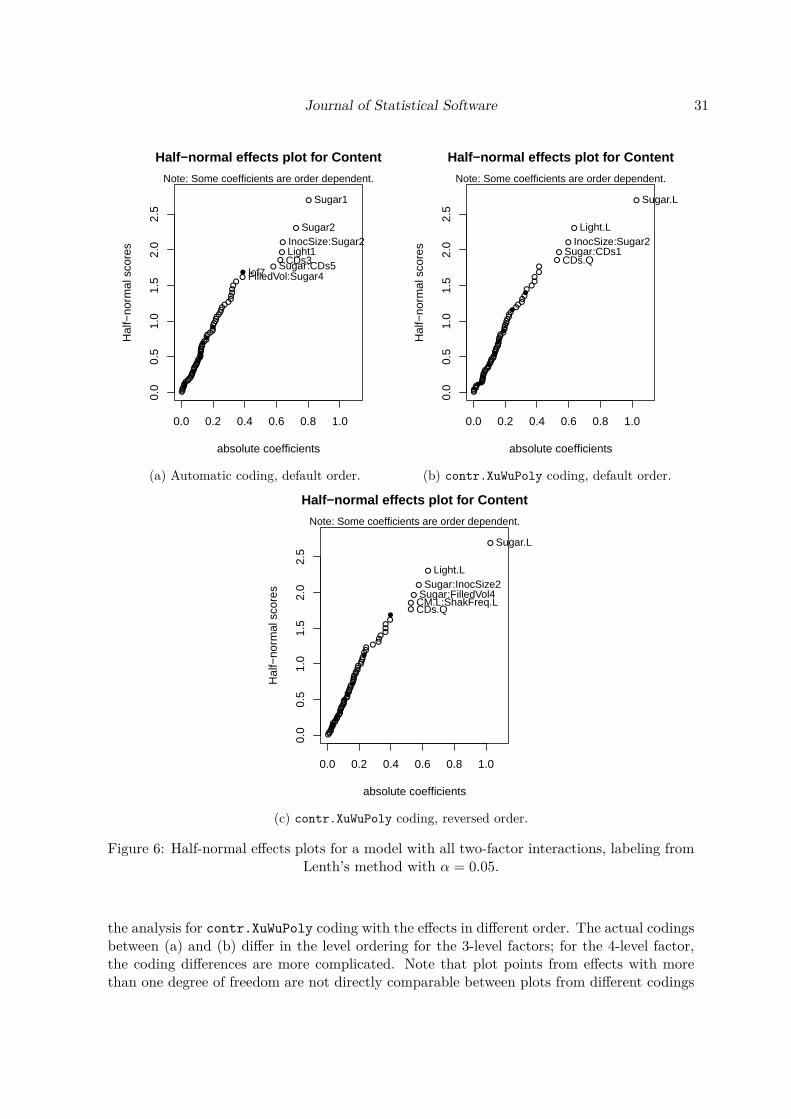
Journal of Statistical Software 31
●●●●●●●●●
●●●●●●●●●●●●●●●●●●●●●●●●●●●●●●●●●●
●●●●●●●●●●●●●●●
●●●●●
●●
●●
●
●
●
●
0.0 0.2 0.4 0.6 0.8 1.0
0.0
0.5
1.0
1.5
2.0
2.5
Half−normal effects plot for Content
absolute coefficients
Hal
f−no
rmal
sco
res
FilledVol:Sugar4 lof7 Sugar:CDs5 CDs3
Light1 InocSize:Sugar2
Sugar2
Sugar1
Note: Some coefficients are order dependent.
(a) Automatic coding, default order.
●●●●●●●●●●
●●●●●●●●●●●●●●●●●●●●●●●●●●●●●●●●●●●●●●●●●●●●
●●●●●●●
●●●
●●
●
●
●
●
●
0.0 0.2 0.4 0.6 0.8 1.0
0.0
0.5
1.0
1.5
2.0
2.5
Half−normal effects plot for Content
absolute coefficients
Hal
f−no
rmal
sco
res
CDs.Q Sugar:CDs1
InocSize:Sugar2 Light.L
Sugar.L
Note: Some coefficients are order dependent.
(b) contr.XuWuPoly coding, default order.
●●●●●●●●●●●●●●●●●●●●●●●●●●●●●●●●●●●●●●●●●●●●●●●●●●
●●●●●●
●●●●
●●●
●●
●●
●
●
●
●
0.0 0.2 0.4 0.6 0.8 1.0
0.0
0.5
1.0
1.5
2.0
2.5
Half−normal effects plot for Content
absolute coefficients
Hal
f−no
rmal
sco
res
CDs.Q CM.L:ShakFreq.L Sugar:FilledVol4 Sugar:InocSize2
Light.L
Sugar.L
Note: Some coefficients are order dependent.
(c) contr.XuWuPoly coding, reversed order.
Figure 6: Half-normal effects plots for a model with all two-factor interactions, labeling fromLenth’s method with α = 0.05.
the analysis for contr.XuWuPoly coding with the effects in different order. The actual codingsbetween (a) and (b) differ in the level ordering for the 3-level factors; for the 4-level factor,the coding differences are more complicated. Note that plot points from effects with morethan one degree of freedom are not directly comparable between plots from different codings

32 DoE.base for Factorial Experiments in R
(e.g., plots (a) and (b) of Figure 6); the comparable message is restricted to the presence orabsence of individual effect components among the top-ranked absolute coefficients (and eventhat may be coding dependent). For the example data, while there are clear visual differencesbetween the differently-coded plots, the message is more or less the same: As already seenin the linear main effects model, light, sugar and CDs are active factors. Furthermore, thesugar by CDs interaction and the inoculum size by sugar interaction seem to have activecomponents. However, the interaction effects are order dependent. The plot with differentinteraction orders brings up three further interactions into the possibly active range and dropsthe sugar by CDs interaction; thus, clearly, one has to be cautious with statements on theseeffects from half-normal effects plots. However, all effects that show up in the half-normaleffects plots have also been at least marginal in the Anova analysis of the previous section.The calculation results have been stored in the following list objects: hnAuto, hnXuWuPoly,and hnXuWuPolyreordered. The list element res indicates which effects have been projectedout from which other effects; furthermore, the results contain the model matrix after orthogo-nalization, and details about the orthogonalization itself. Printed output of orthogonalizationsteps has been suppressed here. The reader is encouraged to check the printed output of thesimple command:
R> hnDemo <- halfnormal(VSGFS, ME.partial = TRUE, plot = FALSE)
which explains how columns of the main effects model matrix stored in
R> mm <- hnDemo$mm[, 2:11]
are obtained from the original model matrix stored (without intercept column) in
R> desnum(VSGFS)[, 1:10]
8. Further developmentsPackage DoE.base tries a balancing act of offering tools both for practitioners with a relativelyweak statistical background and for statistical experts. In order to save the former fromavoidable grave mistakes, the package takes a cautious strategy issuing many warnings, wheredesigns might be improvable or analyses might be inadequate. In various cases, it would bedesirable to avoid unnecessary warnings; for example, there are arrays for which it is knownfrom theoretical work (Butler 2005) that all choices for certain columns are GMA. For thesearrays, warnings for array optimization should be eliminated, which requires some slightlytedious work.The current design catalog covers many situations, but is also limited especially with respectto availability of non-regular designs. Augmenting the catalog with further useful non-regulardesigns is a difficult task and should not be addressed before studying in more detail therelation between recently developed design quality criteria like GR, GRind, ARFT and SCFTand a design’s usefulness for experimentation. Ideally, it should eventually be possible to au-tomate the entire process of obtaining a good experimental design, combining array selectionwith the selection of columns within the array. It would also be good to have an option for

Journal of Statistical Software 33
requesting a design whose main effects model matrix columns are (near) orthogonal to runorder. The latter wishes are, however, quite resource intensive.So far, the design catalog is used for selecting designs and optimizing column choices fromthem. Kuhfeld (2010) makes much more extensive use of the catalog within a SAS softwaremacro suite for creating experimental designs from the arrays in the catalog, specificallycreated with marketing applications in mind (Kuhfeld 2010). Such use can certainly alsobe combined with the catalog in package DoE.base. The dependent package support.CEs(Aizaki 2012) implements choice experiments in R. However, implementing a functionality asflexible as the one offered in the SAS macros by Kuhfeld (2010) would require substantialadditional effort.Package DoE.base also serves as a tool for supporting further theoretical investigations intoaspects like design regularity and new design quality criteria. For example, the work forGrömping and Bailey (2016) was supported by the package, and recent efforts at developingfurther criteria for checking arrays for combinatorial equivalence have been implemented inthe package (Grömping 2018a).Last but not least, the class ‘design’ and infrastructure for it are also available for useby other packages. Authors of other S3-based packages are invited to use it; the methodswithin package DoE.base for its class ‘design’ can be adjusted to accommodate further typesof designs; please inform the package maintainer, if you would like a new type of designincluded into the methods offered.
AcknowledgmentsBoyko Amarov and Hongquan Xu contributed code to the package. Creation of generalizedresolution functionality was partly supported by grant GR 3843/1-1 of Deutsche Forschungs-gemeinschaft. An anonymous reviewer provided valuable suggestions for improving the paper.
References
Aizaki H (2012). “Basic Functions for Supporting an Implementation of Choice Experimentsin R.” Journal of Statistical Software, Code Snippets, 50(2), 1–24. doi:10.18637/jss.v050.c02.
Box GEP, Tyssedal J (1996). “Projective Properties of Certain Orthogonal Arrays.”Biometrika, 83(4), 950–955. doi:10.1093/biomet/83.4.950.
Butler N (2005). “Generalised Minimum Aberration Construction Results for SymmetricalOrthogonal Arrays.” Biometrika, 92(2), 485–491. doi:10.1093/biomet/92.2.485.
Chambers JM, Hastie TJ (1984). Statistical Models in S. Wadsworth & Brooks/Cole, PacificGrove.
Chasalow S (2012). combinat: Combinatorics Utilities. R package version 0.0-8, URL http://CRAN.R-project.org/package=combinat.

34 DoE.base for Factorial Experiments in R
Collings BJ (1984). “Generating the Intrablock and Interblock Subgroups for Confoundingin General Factorial Experiments.” The Annals of Statistics, 12(4), 1500–1509. doi:10.1214/aos/1176346806.
Collings BJ (1989). “Quick Confounding.” Technometrics, 31(1), 107–110. doi:10.2307/1270370.
Daniel C (1959). “Use of Half Normal Plots in Interpreting Two Level Experiments.” Tech-nometrics, 1(4), 311–340. doi:10.2307/1266715.
Deng LY, Tang B (1999). “Generalized Resolution and Minimum Aberration Criteria forPlackett-Burman and Other Nonregular Factorial Designs.” Statistica Sinica, 9(4), 1071–1082.
Edwards DJ, Mee RW (2008). “Empirically Determined p-Values for Lenth t-Statistics.”Journal of Quality Technology, 40(4), 368–380. doi:10.1080/00224065.2008.11917743.
Eendebak P, Schoen E (2010). “Complete Series of Non-Isomorphic Orthogonal Arrays.” URLhttp://pietereendebak.nl/oapage/.
Fox J, Weisberg S (2011). An R Companion to Applied Regression. 2nd edition. Sage, Thou-sand Oaks. URL http://socserv.socsci.mcmaster.ca/jfox/Books/Companion.
Grömping U (2011a). “Relative Projection Frequency Tables for Orthogonal Arrays.” Reportsin Mathematics, Physics and Chemistry 1/2011, Beuth University of Applied SciencesBerlin, Germany.
Grömping U (2011b). “Tutorial for Designing Experiments Using the R Package RcmdrPlu-gin.DoE.” Reports in Mathematics, Physics and Chemistry 4/2011, Beuth University ofApplied Sciences Berlin, Germany.
Grömping U (2013). FrF2.catlg128: Complete Catalogues of Resolution IV 128 Run 2-LevelFractional Factorials up to 24 Factors. R package version 1.2-1, URL https://CRAN.R-project.org/package=FrF2.catlg128.
Grömping U (2014a). “Mosaic Plots Are Useful for Visualizing Low Order Projections ofFactorial Designs.” The American Statistician, 68(2), 108–116. doi:10.1080/00031305.2014.896829.
Grömping U (2014b). RcmdrPlugin.DoE: R Commander Plugin for (Industrial) Design ofExperiments. R package version 0.12-3, URL https://CRAN.R-project.org/package=RcmdrPlugin.DoE.
Grömping U (2014c). “R Package FrF2 for Creating and Analyzing Fractional Factorial 2-Level Designs.” Journal of Statistical Software, 56(1), 1–56. doi:10.18637/jss.v056.i01.
Grömping U (2015). “Augmented Half Normal Effects Plots in the Presence of a Few ErrorDegrees of Freedom.” Quality and Reliability International, 31(7), 1185–1196. doi:10.1002/qre.1842.
Grömping U (2017a). “Frequency Tables for the Coding Invariant Quality Assessment ofFactorial Designs.” IISE Transactions, 49(5), 505–517. doi:10.1080/0740817x.2016.1241458.

Journal of Statistical Software 35
Grömping U (2017b). DoE.wrapper: Wrapper Package for Design of Experiments Function-ality. R package version 0.9, URL https://CRAN.R-project.org/package=DoE.wrapper.
Grömping U (2018a). “Coding Invariance in Factorial Linear Models and a New Tool forAssessing Combinatorial Equivalence of Factorial Designs.” Journal of Statistical Planningand Inference, 193, 1–14. doi:10.1016/j.jspi.2017.07.004.
Grömping U (2018b). DoE.base: Full Factorials, Orthogonal Arrays and Base Utilities forDoE Packages. R package version 1.0, URL https://CRAN.R-project.org/package=DoE.base.
Grömping U, Bailey RA (2016). “Regular Fractions of Factorial Arrays.” In J Kunert,HC Müller, CA Atkinson (eds.), mODa 11 – Advances in Model-Oriented Design and Anal-ysis: Proceedings of the 11th International Workshop in Model-Oriented Design and Analy-sis held in Hamminkeln, Germany, June 12–17, 2016, pp. 143–151. Springer InternationalPublishing, Cham. doi:10.1007/978-3-319-31266-8_17.
Grömping U, Xu H (2014). “Generalized Resolution for Orthogonal Arrays.” The Annals ofStatistics, 42(3), 918–939. doi:10.1214/14-aos1205.
Kobilinsky A, Bouvier A, Monod H (2018). planor: Generation of Regular Factorial Designs.R package version 1.3-9, URL http://CRAN.R-project.org/package=planor.
Kobilinsky A, Monod H, Bailey RA (2017). “Automatic Generation of Generalised RegularFactorial Designs.” Computational Statistics & Data Analysis, 113, 311–329. doi:10.1016/j.csda.2016.09.003.
Kuhfeld W (2010). “Orthogonal Arrays.” URL http://support.sas.com/techsup/technote/ts723.html.
Langsrud Ø (2001). “Identifying Significant Effects in Fractional Factorial MultiresponseExperiments.” Technometrics, 43(4), 415–424. doi:10.1198/00401700152672500.
Larntz K, Whitcomb P (1998). “Use of Replication in Almost Unreplicated Factorials.”Manuscript of a presentation given at the 42nd ASQ Fall Technical conference in Corning,New York, downloaded 2013-04-26, URL http://www.statease.com/pubs/use-of-rep.pdf.
Lawson J (2016). daewr: Design and Analysis of Experiments with R. R package version1.1-7, URL https://CRAN.R-project.org/package=daewr.
Lenth R (1989). “Quick and Easy Analysis of Unreplicated Factorials.” Technometrics, 31(4),469–473. doi:10.1080/00401706.1989.10488595.
Lenth RV (2009). “Response-Surface Methods in R, Using rsm.” Journal of Statistical Soft-ware, 32(7), 1–17. doi:10.18637/jss.v032.i07.
Meyer D, Zeileis A, Hornik K (2006). “The Strucplot Framework: Visualizing Multi-WayContingency Tables with vcd.” Journal of Statistical Software, 17(3), 1–48. doi:10.18637/jss.v017.i03.

36 DoE.base for Factorial Experiments in R
NIST/SEMATECH (2012). “NIST/SEMATECH e-Handbook of Statistical Methods, Sec-tion 3.” Accessed 2015-02-17, URL http://www.itl.nist.gov/div898/handbook/pri/section3/pri33a.htm.
Plackett RL, Burman JP (1946). “The Design of Optimum Multifactorial Experiments.”Biometrika, 33(4), 305–325. doi:10.1093/biomet/33.4.305.
R Development Core Team (2018). R: A Language and Environment for Statistical Computing.R Foundation for Statistical Computing, Vienna, Austria. URL https://www.R-project.org/.
Sarkar D (2008). lattice: Multivariate Data Visualization with R. Springer-Verlag, New York.URL http://lmdvr.R-Forge.R-project.org/.
SAS Institute Inc (2012). JMP Modeling and Multivariate Methods. Cary.Chapter 8, URL https://www.jmp.com/support/downloads/pdf/jmp1002/Modeling-and-Multivariate-Methods.pdf.
SAS Institute Inc (2018). JMP, Version 14. Cary, NC. URL https://www.JMP.com/.
Schoen E, Eendebak P, Nguyen M (2010). “Complete Enumeration of Pure-Level and Mixed-Level Orthogonal Arrays.” Journal of Combinatorial Designs, 18(2), 123–140. doi:10.1002/jcd.20236.
Stat-Ease Inc (2017). Design-Expert, Version 11. URL https://www.statease.com/dx11.html.
Tang B, Deng LY (1999). “Minimum G2-Aberration for Nonregular Fractional FactorialDesigns.” The Annals of Statistics, 27(6), 1914–1926. doi:10.1214/aos/1017939244.
Vasilev N, Schmitz C, Grömping U, Fischer R, Schillberg S (2014). “Assessment of Culti-vation Factors That Affect Biomass and Geraniol Production in Transgenic Tobacco CellSuspension Cultures.” PLOS One, 9(8), 1–7. doi:10.1371/journal.pone.0104620.
Venables B (2013). conf.design: Construction of Factorial Designs. R package version 2.0.0,URL http://CRAN.R-project.org/package=conf.design.
Venables WN, Ripley BD (2002). Modern Applied Statistics with S. 4th edition. Springer-Verlag, New York. doi:10.1007/978-0-387-21706-2.
Wheeler B (2014). AlgDesign: Algorithmic Experimental Design. R package version 1.1-7.3,URL https://CRAN.R-project.org/package=AlgDesign.
Xu H, Cheng SW, Wu CFJ (2004). “Optimal Projective Three-Level Designs for FactorScreening and Interaction Detection.” Technometrics, 46(3), 280–292. doi:10.1198/004017004000000310.
Xu H, Wu CFJ (2001). “Generalized Minimum Aberration for Asymmetrical Fractional Facto-rial Designs.” The Annals of Statistics, 29(4), 1066–1077. doi:10.1214/aos/1013699993.

Journal of Statistical Software 37
A. Class ‘design’ and functionality for it
Generally, all design generating functions from packages DoE.base and FrF2 (exceptions high-lighted in the documentation) create an output design that is of S3 class ‘design’ and thusthe output follows a certain structure (cf. Section A.1) and allows application of certain in-spection, modification and analysis methods and functions. The first subsection describes theclass ‘design’ itself, the second subsection functionality applicable to class ‘design’ objects.Experimental design matrices or data frames created with tools that do not output class‘design’ objects can be brought into that class by function data2design, in order to makesome of the package functionality work on them.
A.1. Class ‘design’
An object of S3 class ‘design’ is a a data frame with the three attributes "desnum", "run.order"and "design.info".
• Attribute "desnum" can be used for a numeric version of the data frame, which may beuseful for users who want to do manual matrix calculations. The package functionalityitself makes little use of that attribute.
• Attribute "run.order" has the main purpose of always being able to switch back andforth between a standard order and the randomized run order.
• Attribute "design.info" is a list that contains all the important information on thedesign and is heavily used by the methods and functions discussed in the followingsubsection. This attribute will be described in some detail in the rest of this subsection.
The "design.info" attribute has some mandatory elements that have to be present for allclass ‘design’ objects and many elements that are needed for some types of designs only.The author’s website contains a large table that details which types of designs need whichelements of the "design.info" attribute. Tables 2, 3 and 4 list the elements and theirmeaning/context.Apart from the elements listed in the table, there are further elements for class ‘design’objects created by design combination functions. These are not discussed here. For suchdesigns, the entry types given in the table can also be replaced by lists of several such entries.
A.2. Functionality for class ‘design’ objects
Package DoE.base offers inspection functionality (print, summary, plot as methods for theirgenerics, corrPlot as a standalone function) and analysis methods (plot, lm, halfnormal) forthis class, as well as a sub-setting method using [, which is useful for reordering experimentalruns (to switch between standard order and randomized order, to re-randomize).Besides these major functions, there are various further functions tailored to the need of class‘design’ objects, either as methods for generic functions or just as functions:

38 DoE.base for Factorial Experiments in R
Element Data type RoleMandatory elements
type character string identifies the type of designnruns number number of runs (replications not counted)nfactors number number of factorsfactor.names named list factor names and factor levels (or scale ends for
quantitative factors)replications number number of replications or repeated measure-
ments per runrepeat.only logical if TRUE, the number given in the replications el-
ement refers to repeated measurements onlyrandomize logical if TRUE, run order has been randomizedseed number the seed used for randomizationcreator call or list of menu
settings in GUIthe creation history of the object
Optional general elementsresponse.names vector of character
stringsnames of the response columns (column namesfrom the data frame)
Elements for blocked designs (from functions fac.design, rerandomize.design,or FrF2)
block.name character string name of block variablenblocks number number of blocksblock.gen number Yates matrix column number(s) of factor(s) used
for blocking (FrF2) or block generator matrix(fac.design)
blocksize number run size of each block (without replications)bbreps number number of between block replications (identical
to replications)wbreps number number of within block replications (these can
be proper replications or repeated measure-ments only)
Further element for full factorial designs and orthogonal array designs (functionsfac.design or oa.design)
nlevels numeric vector withnfactors elements
number of levels for each factor
Further elements for general orthogonal array based designs (function oa.design)generating.oa character string name of the OA used (from catalog of orthogonal
arrays or user-provided)selected.columns numeric vector with
nfactors elementscolumn number from generating.oa for eachfactor
origin character string origin specification from generating.oa(empty, if there is none)
comment character string comment from generating.oa (empty, if thereis none)
residual.df number residual degrees of freedom for main effects onlyanalysis
Table 2: Elements of the "design.info" attribute of class ‘design’ – Part I.

Journal of Statistical Software 39
Element Data type RoleFurther element for designs created by function pb
ndummies number number of columns not assigned to experimentalfactors
Further elements for designs created by function FrF2aliased list with character el-
ementsinformation on the alias structure of the designup to degree 2
FrF2.version character string version number of package FrF2, when designwas created
generators character vector ordesign key matrix
design generators in the format “D = ABC”etc. for FrF2 designs or design key matrix fordesigns created with package planor
catlg.name character string name of the catalog used for design creationcatlg.entry list of length 1 of
class ‘catlg’the catalog entry used for the design
ntreat number identical to nfactors, present for blocked de-signs for historical reasons
aliased.with.blocks
character vector lists two-factor interactions that are aliased withthe block main effect
base.design character string element of design catalog used for creating ablocked or split plot design from
nfac.WP number number of whole plot factorsnfac.SP number number of split plot factorsnWPs number number of whole plotsplotsize number run size of each plot (without replications)res.WP number resolution of the whole plot portion of the designmap numeric vector with
k elementsmapping of base factors so that estimability orrandomization restriction requirement is fulfilled
orig.fac.order numeric vector withnfactors elements
order of original factors from function call forsplit plot designs
clear logical if TRUE, the design is clear (for estimability re-quirement)
res3 logical if TRUE, resolution III has been permitted forestimability request
quantitative logical vector withnfactors elements
TRUE elements indicate quantitative factors
ncube number number of cube points in a design with centerpoints
ncenter number number of center pointscoding list of formulae coding of quantitative factors (for use with pack-
age rsm; Lenth 2009)
Table 3: Elements of the "design.info" attribute of class ‘design’ – Part II.

40 DoE.base for Factorial Experiments in R
Element Data type RoleFurther elements for designs created by function Dopt.design
The function also outputs the split plot related elements and elementquantitative described under specific elements for FrF2 above.plot.name character string name of whole plot factor in split plot re-
questdigits number number of digits to which quantitative fac-
tors are to be roundedformula formula model formula for which D-optimality is to
be achievedconstraint logical expression constraint applied to the experimental fac-
torsoptimality.criteria named numeric vec-
torperformance of design on several optimalitycriteria
Further elements for designs created by function lhs.designsubtype character string type of latin hypercube designThe function also outputs digits and optimality.criteria elements de-scribed under specific elements for Dopt.design above.
Table 4: Elements of the "design.info" attribute of class ‘design’ – Part III.
• Functions design.info, run.order, and desnum extract or set the respective attributesof a class ‘design’ object.
• Functions factor.names and response.names get or set the respective element fromthe "design.info" attribute.
• Function generators extracts generating information for designs of type FrF2 or planor.
• Function getblock extracts block information for replicated designs (see also Section 2).
• Function rerandomize.design allows to re-randomize a class ‘design’ object with-out response data; this also allows explicit blocking of designs created with functionsoa.design and pb (see also Section 5.3).
• Functions for designs that can be both in wide or in long format, i.e., parameter designsand designs with repeated measurements, can change between long and wide formator aggregate wide format designs: Function rep2wide brings repeated measurementdesigns into wide format, reptolong does the opposite; function paramtowide bringsa parameter design to wide format (irreversible, they are created in long format); theaggregate method for ‘design’ objects aggregates designs in wide format into designswith a single response.
• Functions add.response and col.remove add responses or remove columns; functionresponse.names can also be used to remove response columns.
• Function qua.design influences, which design columns are quantitative, and functionchange.contr changes the contrasts of design columns.

Journal of Statistical Software 41
• Functions undesign and redesign remove the class ‘design’ properties from an objector reinstate them. Using function data2design instead of redesign on the result ofundesign allows to treat a block factor as a normal experimental factor without a specialrole (see Section 5.3).
• Functions cross.design and param.design combine class ‘design’ objects into crosseddesigns or parameter designs, respectively.
• The fix method for ‘design’ objects has been adapted from package utils; it allows toedit ‘design’ objects; however, its use is not recommended.
• Function export.design can export a design in HTML or CSV format, together withan R workspace for the design. After entering response data in a spreadsheet program,responses can be added to the design itself using the add.response function.
Affiliation:Ulrike GrömpingDepartment II – Mathematics, Physics, ChemistryBeuth University of Applied Sciences BerlinD-13353 Berlin, GermanyE-mail: [email protected]: http://prof.beuth-hochschule.de/groemping/
Journal of Statistical Software http://www.jstatsoft.org/published by the Foundation for Open Access Statistics http://www.foastat.org/June 2018, Volume 85, Issue 5 Submitted: 2015-04-27doi:10.18637/jss.v085.i05 Accepted: 2017-08-14