causal interaction in factorial experiments: …imai.princeton.edu/research/files/int.pdfcausal...
TRANSCRIPT

Causal Interaction in Factorial Experiments:
Application to Conjoint Analysis∗
Naoki Egami† Kosuke Imai‡
Forthcoming in Journal of the American Statistical Association
Abstract
We study causal interaction in factorial experiments, in which several fac-
tors, each with multiple levels, are randomized to form a large number of pos-
sible treatment combinations. Examples of such experiments include conjoint
analysis, which is often used by social scientists to analyze multidimensional
preferences in a population. To characterize the structure of causal interaction
in factorial experiments, we propose a new causal interaction effect, called the
average marginal interaction effect (AMIE). Unlike the conventional interaction
effect, the relative magnitude of the AMIE does not depend on the choice of
baseline conditions, making its interpretation intuitive even for higher-order in-
teractions. We show that the AMIE can be nonparametrically estimated using
ANOVA regression with weighted zero-sum constraints. Because the AMIEs
are invariant to the choice of baseline conditions, we directly regularize them by
collapsing levels and selecting factors within a penalized ANOVA framework.
This regularized estimation procedure reduces false discovery rate and further
facilitates interpretation. Finally, we apply the proposed methodology to the
conjoint analysis of ethnic voting behavior in Africa and find clear patterns of
causal interaction between politicians’ ethnicity and their prior records. The
proposed methodology is implemented in an open source software package.
Key words: ANOVA, causal inference, heterogeneous treatment effects, in-
teraction effects, randomized experiments, regularization
∗The proposed methods are implemented through open-source software FindIt: Finding Hetero-geneous Treatment Effects (Egami et al., 2017), which is freely available as an R package at the
Comprehensive R Archive Network (CRAN http://cran.r-project.org/package=FindIt). We thank
Elizabeth Carlson for providing us with data and answering our questions. We are also grate-
ful for Jens Hainmueller, Walter Mebane, Dustin Tingley, Teppei Yamamoto, Tyler VanderWeele,
and seminar participants at Carnegie Mellon University (Statistics), Georgetown University (School
of Public Policy), Stanford (Political Science), Umea University (Statistics), University of Bristol
(Mathematics), and UCLA (Political Science) for helpful comments on an earlier version of the
paper.†Ph.D. student, Department of Politics, Princeton University, Princeton NJ 08544. Email:
[email protected], URL: http://scholar.princeton.edu/negami‡Professor, Department of Politics and Center for Statistics and Machine Learning, Prince-
ton University, Princeton NJ 08544. Phone: 609–258–6601, Email: [email protected], URL:
https://imai.princeton.edu

1 Introduction
Statistical interaction among treatment variables can be interpreted as causal rela-
tionships when the treatments are randomized in an experiment. Causal interaction
plays an essential role in the exploration of heterogeneous treatment effects. This pa-
per develops a framework for studying causal interaction in randomized experiments
with a factorial design, in which there are multiple factorial treatments with each
having several levels. A primary goal of causal interaction analysis is to identify the
combinations of treatments that induce large additional effects beyond the sum of
effects separately attributable to each treatment.
Our motivating application is conjoint analysis, which is a type of randomized
survey experiment with a factorial design (Luce and Tukey, 1964). Conjoint analysis
has been extensively used in marketing research to investigate consumer preferences
and predict product sales (e.g., Green et al., 2001; Marshall and Bradlow, 2002). In a
typical conjoint analysis, respondents are asked to evaluate pairs of product profiles
where several characteristics of a commercial product such as price and color are
randomly chosen. Because these product characteristics are represented by factorial
variables, conjoint analysis can be seen as an application of randomized factorial
design. Thus, the causal estimands and estimation methods proposed in this paper
are widely applicable to any factorial experiments with many factors.
Recently, conjoint analysis has also gained its popularity among medical and social
scientists who study multidimensional preferences among a population of individuals
(e.g., Marshall et al., 2010; Hainmueller and Hopkins, 2015). In this paper, we focus
on the latter use of conjoint analysis by estimating population average causal effects.
Specifically, we analyze a conjoint analysis about coethnic voting in Africa to examine
the conditions under which voters prefer political candidates of the same ethnicity (see
Section 2 for the details of the experiment and Section 6 for our empirical analysis).
1

One important limitation of conjoint analysis, as currently conducted in applied
research, is that causal interactions are largely ignored. This is unfortunate because
studies of multi-dimensional choice necessarily involve the consideration of interaction
effects. However, the exploration of causal interactions in conjoint analysis is often
difficult for two reasons. First, the relative magnitude of the conventional causal
interaction effect depends on the choice of baseline condition. This is problematic
because many factors used in conjoint analysis do not have natural baseline conditions
(e.g., gender, racial group, religion, occupation). Second, a typical conjoint analysis
has several factors with each having multiple levels. This means that we must apply a
regularization method to reduce false discovery and facilitate interpretation. Yet, the
lack of invariance property means that the results of standard regularized estimation
will depend on the choice of baseline conditions.
To overcome these problems, we propose an alternative definition of causal inter-
action effect that is invariant to the choice of baseline condition, making its inter-
pretation intuitive even for higher-order interactions (Sections 3 and 4). We call this
new causal quantity of interest, the average marginal interaction effect (AMIE), be-
cause it marginalizes the other treatments rather than conditioning on their baseline
values as done in the conventional causal interaction effect. The proposed approach
enables researchers to effectively summarize the structure of causal interaction in
high-dimension by decomposing the total effect of any treatment combination into
the separate effect of each treatment and their interaction effects.
Finally, we also establish the identification condition and develop estimation
strategies for the AMIE (Section 5). We propose a nonparametric estimator of the
AMIE and show that this estimator can be recast as an ANOVA with weighted zero-
sum constraints (Scheffe, 1959). Exploiting this equivalence relationship, we apply
the method proposed by Post and Bondell (2013) and directly regularize the AMIEs
2

within the ANOVA framework by collapsing levels and selecting factors. Because the
AMIE is invariant to the choice of baseline condition, our regularization also has the
same invariance property. This also enables a proper regularization of the conditional
average effects, which can be computed using the AMIEs. Without the invariance
property, the results of regularized estimation will depend on the choice of baseline
conditions. All of our theoretical results and estimation strategies are shown to hold
for causal interaction of any order. The proposed methodology is implemented via an
open-source software package, FindIt: Finding Heterogeneous Treatment Effects (Egami
et al., 2017), which is available for download at the Comprehensive R Archive Network
(CRAN; https://cran.r-project.org/package=FindIt).
Our paper builds on the causal inference and experimental design literatures that
are concerned about interaction effects (see e.g., Cox, 1984; Jaccard and Turrisi, 2003;
de Gonzalez and Cox, 2007; VanderWeele and Knol, 2014). In addition, we draw upon
the recent papers that provide the potential outcomes framework for causal inference
with factorial experiments and conjoint analysis (Dasgupta et al., 2015; Hainmueller
et al., 2014; Lu, 2016a,b). Indeed, the AMIE is a direct generalization of the average
marginal effect studied in this literature that can be used to characterize the causal
heterogeneity of a high-dimensional treatment.
Finally, this paper is also related to the literature on heterogeneous treatment
effects, in which the goal of analysis is to find an optimal treatment regime. Much
of this literature, however, focuses on the interaction between a single treatment and
pre-treatment covariates (e.g., Hill, 2012; Green and Kern, 2012; Wager and Athey,
2017; Grimmer et al., 2017) or a dynamic setting where a sequence of treatment
decisions is optimized (e.g., Murphy, 2003; Robins, 2004). We emphasize that if the
goal of analysis is to find an optimal treatment regime, rather than to understand
the structure of causal heterogeneity, the marginalized causal quantities such as the
3

Factors LevelsCoethnicity Yes a coethnic of a respondent
No not a coethnic of a respondentRecord Yes/Village politician for a village with good prior record
Yes/District politician for a district with good prior recordYes/MP member of parliament with good prior recordNo/Village politician for a village without good prior recordNo/District politician for a district without good prior recordNo/MP member of parliament without good prior recordNo/Business businessman without good prior record
Platform Job promise to create new jobsClinic promise to create clinicsEducation promise to improve education
Degree Yes masters degree in business, law, economics, or developmentNo bachelors degree in tourism, horticulture, forestry or theater
Table 1: Levels of Four Factors from the Conjoint Analysis in Carlson (2015).
one proposed in this paper may be of little use. In such settings, researchers typically
estimate the causal effects of specific treatment combinations (e.g., Imai and Ratkovic,
2013).
2 Conjoint Analysis of Ethnic Voting
Conjoint analysis has a long history dating back to the theoretical paper by Luce
and Tukey (1964). In terms of its application, it has been widely used by marketing
researchers over the last 40 years to measure consumer preferences and predict product
sales (Green and Rao, 1971; Green et al., 2001; Marshall and Bradlow, 2002). It has
also become a popular statistical tool in the medical and social sciences (e.g., Marshall
et al., 2010; Hainmueller and Hopkins, 2015) to study multidimensional preferences
of a variety of populations such as patients and voters.
Conjoint analysis can be considered as an application of factorial randomized ex-
periments. For example, in a typical conjoint analysis used for marketing research,
respondents evaluate a commercial product whose several characteristics such as price
and color etc. are randomly selected. Factorial variables represent these characteris-
tics with several levels (e.g., $1, $5, $10 for price, and red, green, and blue for color).
4

Similarly, in political science research, conjoint analysis may be used to evaluate can-
didates where factors may represent their party identification, race, gender, and other
attributes.
In this paper, we examine a recent conjoint analysis conducted to study coeth-
nic voting in Uganda (Carlson, 2015). Coethnic voting refers to the tendency of
some voters to prefer political candidates whose ethnicity is the same as their own.
Researchers have observed that coethnic voting occurs frequently among African vot-
ers, but the identification of causal effects is often difficult because the ethnicity of
candidates are often correlated with other characteristics that may influence voting
behavior. To address this problem, the original author conducted a conjoint analysis,
in which respondents were asked to choose one of the two hypothetical candidates
whose attributes were randomly assigned.
For the experiment, a total of 547 respondents were sampled from villages in
Uganda. We analyze a subset of 544 observations after removing 3 observations with
missing data. Each respondent was given the description of three pairs of hypothetical
presidential candidates. They were then asked to cast a vote for one of the candidates
within each pair. These hypothetical candidates are characterized by a total of four
factors shown in Table 1: Coethnicity (2 levels), Record (7 levels), Platform (3
levels), and Degree (2 levels).
While the levels of all factors are randomly and independently selected for each
hypothetical candidate, the distribution of candidate ethnicity depends on the local
ethnic diversity so that enough respondents share the same ethnicity as their assigned
hypothetical candidates. The original analysis was based on a mixed effects logistic
regression with a respondent random effect. While previous studies showed that
many voters unconditionally favor coethnic candidates, Carlson (2015) found that
voters tend to favor only coethnic candidates with good prior record.
5
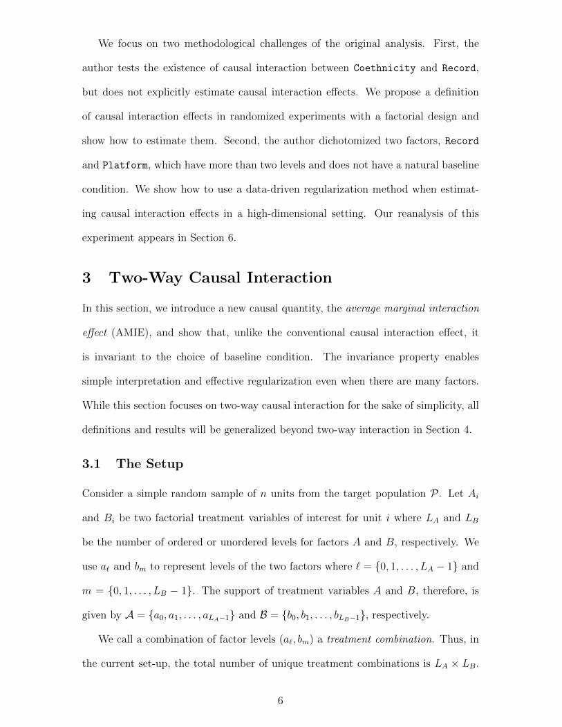
We focus on two methodological challenges of the original analysis. First, the
author tests the existence of causal interaction between Coethnicity and Record,
but does not explicitly estimate causal interaction effects. We propose a definition
of causal interaction effects in randomized experiments with a factorial design and
show how to estimate them. Second, the author dichotomized two factors, Record
and Platform, which have more than two levels and does not have a natural baseline
condition. We show how to use a data-driven regularization method when estimat-
ing causal interaction effects in a high-dimensional setting. Our reanalysis of this
experiment appears in Section 6.
3 Two-Way Causal Interaction
In this section, we introduce a new causal quantity, the average marginal interaction
effect (AMIE), and show that, unlike the conventional causal interaction effect, it
is invariant to the choice of baseline condition. The invariance property enables
simple interpretation and effective regularization even when there are many factors.
While this section focuses on two-way causal interaction for the sake of simplicity, all
definitions and results will be generalized beyond two-way interaction in Section 4.
3.1 The Setup
Consider a simple random sample of n units from the target population P . Let Ai
and Bi be two factorial treatment variables of interest for unit i where LA and LB
be the number of ordered or unordered levels for factors A and B, respectively. We
use a` and bm to represent levels of the two factors where ` = {0, 1, . . . , LA − 1} and
m = {0, 1, . . . , LB − 1}. The support of treatment variables A and B, therefore, is
given by A = {a0, a1, . . . , aLA−1} and B = {b0, b1, . . . , bLB−1}, respectively.
We call a combination of factor levels (a`, bm) a treatment combination. Thus, in
the current set-up, the total number of unique treatment combinations is LA × LB.
6

Let Yi(a`, bm) denote the potential outcome variable of unit i if the unit receives the
treatment combination (a`, bm). For each unit, only one of the potential outcome
variables can be observed, and the realized outcome variable is denoted by Yi =∑a`∈A,bm∈B 1{Ai = a`, Bi = bm}Yi(a`, bm), where 1{Ai = a`, Bi = bm} is an indicator
variable taking the value 1 when Ai = a` and Bi = bm, and taking the value 0
otherwise. In this paper, we make the stability assumption, which states that there is
neither interference between units nor different versions of the treatment (Cox, 1958;
Rubin, 1990).
In addition, we assume that the treatment assignment is randomized.
{Yi(a`, bm)}a`∈A,bm∈B ⊥⊥ {Ai, Bi} for all i = 1, . . . , n. (1)
Pr(Ai = a`, Bi = bm) > 0 for all a` ∈ A and bm ∈ B. (2)
This assumption rules out the use of fractional factorial designs where certain com-
binations of treatments have zero probability of occurrence. In some cases, however,
researchers may wish to eliminate certain treatment combinations for substantive
reasons. The standard recommendation is to set the probability for those treatment
combinations to small non-zero values under a full factorial design so that the assump-
tion continues to hold (see Hainmueller et al., 2014, footnote 18). Another possibility
is to restrict one’s analysis to a subset of data and hence the corresponding subset of
estimands so that the assumption is satisfied.
Under this setup, we review two non-interactive causal effects of interest. First,
we define the average combination effect (ACE), which represents the average causal
effect of a treatment combination (Ai, Bi) = (a`, bm) relative to a pre-specified baseline
condition (a0, b0) (e.g., Dasgupta et al., 2015).
τAB(a`, bm; a0, b0) ≡ E{Yi(a`, bm)− Yi(a0, b0)}, (3)
where a`, a0 ∈ A and bm, b0 ∈ B.
7
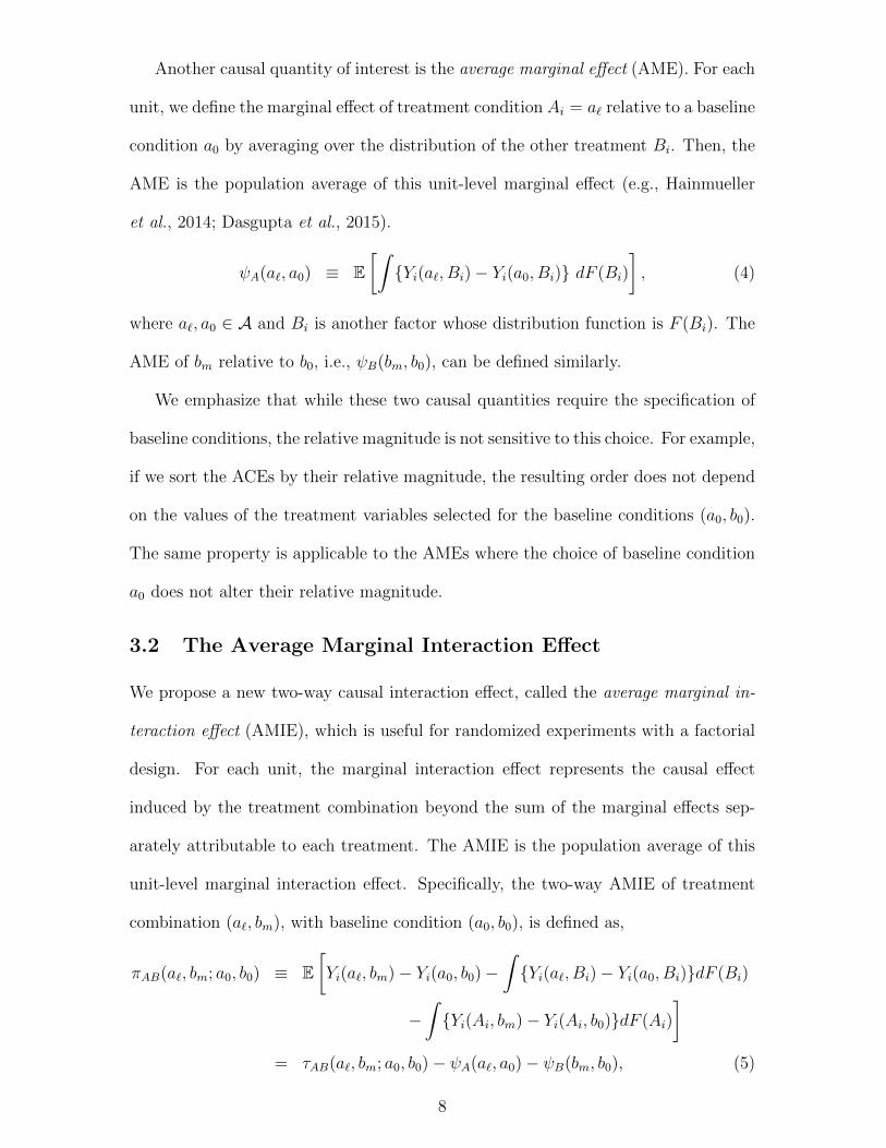
Another causal quantity of interest is the average marginal effect (AME). For each
unit, we define the marginal effect of treatment condition Ai = a` relative to a baseline
condition a0 by averaging over the distribution of the other treatment Bi. Then, the
AME is the population average of this unit-level marginal effect (e.g., Hainmueller
et al., 2014; Dasgupta et al., 2015).
ψA(a`, a0) ≡ E[∫{Yi(a`, Bi)− Yi(a0, Bi)} dF (Bi)
], (4)
where a`, a0 ∈ A and Bi is another factor whose distribution function is F (Bi). The
AME of bm relative to b0, i.e., ψB(bm, b0), can be defined similarly.
We emphasize that while these two causal quantities require the specification of
baseline conditions, the relative magnitude is not sensitive to this choice. For example,
if we sort the ACEs by their relative magnitude, the resulting order does not depend
on the values of the treatment variables selected for the baseline conditions (a0, b0).
The same property is applicable to the AMEs where the choice of baseline condition
a0 does not alter their relative magnitude.
3.2 The Average Marginal Interaction Effect
We propose a new two-way causal interaction effect, called the average marginal in-
teraction effect (AMIE), which is useful for randomized experiments with a factorial
design. For each unit, the marginal interaction effect represents the causal effect
induced by the treatment combination beyond the sum of the marginal effects sep-
arately attributable to each treatment. The AMIE is the population average of this
unit-level marginal interaction effect. Specifically, the two-way AMIE of treatment
combination (a`, bm), with baseline condition (a0, b0), is defined as,
πAB(a`, bm; a0, b0) ≡ E[Yi(a`, bm)− Yi(a0, b0)−
∫{Yi(a`, Bi)− Yi(a0, Bi)}dF (Bi)
−∫{Yi(Ai, bm)− Yi(Ai, b0)}dF (Ai)
]= τAB(a`, bm; a0, b0)− ψA(a`, a0)− ψB(bm, b0), (5)
8

where a`, a0 ∈ A and bm, b0 ∈ B, πAB(a`, bm; a0, b0) is the AMIE, and ψ(·, ·) is the
AME defined in equation (4).
The AMIE is closely connected to the conventional definition of the average inter-
action effect (AIE). In the causal inference literature (e.g., Cox, 1984; VanderWeele,
2015; Dasgupta et al., 2015), researchers define the AIE of treatment combination
(a`, bm) relative to baseline condition (a0, b0) as,
ξAB(a`, bm; a0, b0) ≡ E{Yi(a`, bm)− Yi(a0, bm)− Yi(a`, b0) + Yi(a0, b0)}, (6)
where a`, a0 ∈ A and bm, b0 ∈ B.
Similar to the AMIE, the AIE has an interactive effect interpretation, representing
the additional average causal effect induced by the treatment combination beyond
the sum of the average causal effects separately attributable to each treatment. This
interpretation is based on the following algebraic equality,
ξAB(a`, bm; a0, b0) = τAB(a`, bm; a0, b0)−E{Yi(a`, b0)−Yi(a0, b0)}−E{Yi(a0, bm)−Yi(a0, b0)}.
(7)
The difference between the AMIE and the AIE is that the former subtracts the
AMEs from the ACE while the latter subtracts the sum of two separate effects due
to Ai = a` and Bi = bm while holding the other treatment variable at its baseline
value, i.e., Ai = a0 or Bi = b0.
In addition, the AIE has a conditional effect interpretation,
ξAB(a`, bm; a0, b0) = E{Yi(a`, bm)− Yi(a0, bm)} − E{Yi(a`, b0)− Yi(a0, b0)},
which denotes the difference in the average causal effect of Ai = a` relative to Ai = a0
between the two scenarios, one when Bi = bm and the other when Bi = b0. When
such conditional effects are of interest, the AMIE can be used to obtain them. For
example, we have,
E{Yi(a`, b0)− Yi(a0, b0)} = ψA(a`; a0) + πAB(a`, b0; a0, b0). (8)
9
Clearly, the scientific question of interest should determine the choice between the
AMIE and AIE. In Section 6, we illustrate how to use the AMIEs for estimating the
average conditional effects when necessary.
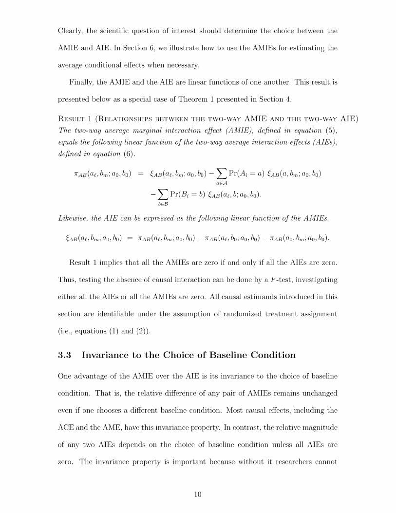
Finally, the AMIE and the AIE are linear functions of one another. This result is
presented below as a special case of Theorem 1 presented in Section 4.
Result 1 (Relationships between the two-way AMIE and the two-way AIE)
The two-way average marginal interaction effect (AMIE), defined in equation (5),
equals the following linear function of the two-way average interaction effects (AIEs),
defined in equation (6).
πAB(a`, bm; a0, b0) = ξAB(a`, bm; a0, b0)−∑a∈A
Pr(Ai = a) ξAB(a, bm; a0, b0)
−∑b∈B
Pr(Bi = b) ξAB(a`, b; a0, b0).
Likewise, the AIE can be expressed as the following linear function of the AMIEs.
ξAB(a`, bm; a0, b0) = πAB(a`, bm; a0, b0)− πAB(a`, b0; a0, b0)− πAB(a0, bm; a0, b0).
Result 1 implies that all the AMIEs are zero if and only if all the AIEs are zero.
Thus, testing the absence of causal interaction can be done by a F -test, investigating
either all the AIEs or all the AMIEs are zero. All causal estimands introduced in this
section are identifiable under the assumption of randomized treatment assignment
(i.e., equations (1) and (2)).
3.3 Invariance to the Choice of Baseline Condition
One advantage of the AMIE over the AIE is its invariance to the choice of baseline
condition. That is, the relative difference of any pair of AMIEs remains unchanged
even if one chooses a different baseline condition. Most causal effects, including the
ACE and the AME, have this invariance property. In contrast, the relative magnitude
of any two AIEs depends on the choice of baseline condition unless all AIEs are
zero. The invariance property is important because without it researchers cannot
10

systematically compare interaction effects of different treatment combinations. We
state this as Result 2, which is a special case of Theorem 2 presented in Section 5.
Result 2 (Invariance and Lack Thereof to the Choice of Baseline Condition)
The average marginal interaction effect (AMIE), defined in equation (5), is interval
invariant. That is, for any (a`, bm) 6= (a`′ , bm′) and (a0, b0) 6= (a˜, bm), the following
equality holds,
πAB(a`, bm; a0, b0) − πAB(a`′ , bm′ ; a0, b0) = πAB(a`, bm; a˜, bm) − πAB(a`′ , bm′ ; a˜, bm).
Note that the above difference of the AMIEs is also equal to another AMIE, πAB(a`, bm; a`′ , bm′).
In contrast, the average interaction effect (AIE), defined in equation (6) does not
have the invariance property. That is, the following equality does not generally hold,
ξAB(a`, bm; a0, b0)− ξAB(a`′ , bm′ ; a0, b0) = ξAB(a`, bm; a˜, bm)− ξAB(a`′ , bm′ ; a˜, bm).
In addition, the AIE is interval invariant if and only if all the AIEs are zero.
The sensitivity of the AIEs to the choice of baseline condition can be further
illustrated by the fact that the AIE of any treatment combination pertaining to
one of levels in the baseline condition is equal to zero. That is, if (a0, b0) is the
baseline condition, then ξAB(a0, bm; a0, b0) = ξAB(a`, b0; a0, b0) = 0. If the researchers
are only interested in the conditional effect interpretation of the AIEs, these zero
AIEs are not of interest. However, this restriction is problematic for the interactive
effect interpretation especially when no natural baseline condition exists. In such
circumstances, zero AIEs make it impossible to explore all relevant causal interaction
effects. To the contrary, researchers need not to restrict their quantities of interest
when using the AMIE, which can take a non-zero value even when one treatment is
set to the baseline condition. For example, the AMIE can be positive if the effect of
the second treatment is large when the first treatment is set to its baseline value.
While it is invariant to the choice of baseline condition, the AMIE critically de-
pends on the distribution of treatments, i.e., P (A,B). This is because the AMIE is
a function of the AMEs, which are themselves obtained by marginalizing out other
treatments. This dependency of causal quantities is not new. The potential outcomes
11

framework for 2k factorial experiments introduced by Dasgupta et al. (2015), for ex-
ample, defines causal estimands based on the uniform distribution of treatments.
Many applied researchers independently randomize multiple treatments and then es-
timate the AME of each treatment by simply ignoring the other treatments. This
estimation procedure implicitly conditions on the empirical distribution of treatment
assignments.
Although the uniform or empirical distribution would be a reasonable default
choice for many experimentalists, researchers can improve the external validity of
their experiment by using a treatment distribution based on the target population
(Hainmueller et al., 2014). This is important for the conjoint analysis, in which treat-
ments are often characteristics of people. In our empirical application (see Section 2),
for example, researchers could obtain the detailed information about the attributes
of actual candidates and use it as the basis of treatment distribution.
4 Generalization to Higher Order Interaction
In this section, we generalize the two-way AMIE introduced in Section 3 to higher
order causal interaction with more than two factors. We prove that a higher order
AMIE retains the same desirable properties and intuitive interpretation.
4.1 The Setup
Suppose that we have a total of J factorial treatments denoted by an vector Ti =
(Ti1, Ti2, . . . , TiJ) where J ≥ 2 and each factor Tij has a total of Lj levels. Without loss
of generality, let T1:Ki be a subset of K treatments of interest where K ≤ J whereas
T(K+1):Ji denotes the remaining (J −K) factorial treatment variables, which are not
of interest. As before, we assume that the treatment assignment is randomized.
Assumption 1 (Randomized Treatment Assignment)
Yi(t) ⊥⊥ Ti and Pr(Ti = t) > 0 for all t.
12

In addition, we assume that J factorial treatments are independent of one another.
Assumption 2 (Independent Treatment Assignment)
Tij ⊥⊥ Ti,−j for all j ∈ {1, 2, . . . , J},
where Ti,−j denotes the (J − 1) factorial treatments excluding Tij.
Assumption 2 is not required for some of the results obtained below, but it consider-
ably simplifies the notation.
We now generalize the definition of the two-way ACE given in equation (3) by
accommodating more than two factorial treatments of interest T1:Ki while allowing
for the existence of additional treatments T(K+1):Ji , which are marginalized out.
Definition 1 (The K-way Average Combination Effect) The K-way aver-
age combination effect (ACE) of treatment combination T1:Ki = t1:K relative to base-
line condition T1:Ki = t1:K0 is defined as,
τ1:K(t1:K ; t1:K0 ) ≡ E[∫ {
Yi(T1:Ki = t,T
(K+1):Ji )− Yi(T1:K
i = t1:K0 ,T(K+1):Ji )
}dF (T
(K+1):Ji )
].
The generalization of the AME defined in equation (4) to this setting is straight-
forward. For example, the AME of Ti1 is obtained by marginalizing the remaining
factors T2:Ji out.
4.2 The K-way Average Marginal Interaction Effect
We now extend the definition of the two-way AMIE, given in equation (5), to higher-
order causal interaction and discuss its relationships with the conventional higher-
order causal interaction effect. We define the K-way AMIE as the additional effect
of treatment combination beyond the sum of all lower-order AMIEs.
Definition 2 (The K-way Average Marginal Interaction Effect) The K-
way average marginal interaction effect (AMIE) of treatment combination T1:Ki =
t1:K, relative to baseline condition, T1:Ki = t1:K0 , is given by,
π1:K(t1:K ; t1:K0 ) ≡ E
{τ(i)1:K(t1:K ; t1:K0 )−
K−1∑k=1
∑Kk⊆KK
π(i)Kk
(tKk ; tKk0 )
}
13

= τ1:K(t1:K ; t1:K0 )−K−1∑k=1
∑Kk⊆KK
πKk(tKk ; tKk
0 ),
where Kk ⊆ KK = {1, . . . , K} such that |Kk| = k with k = 1, . . . , K, τ(i)1:K(t1:K ; t1:K0 ) is
the unit-level combination effect, and π(i)1:K(t1:K ; t1:K0 ) is the unit-level K-way marginal
interaction effect.
This definition reduces to equation (5) when K = 2 because the one-way AMIE is
equal to the AME, i.e., π1(t; t0) = ψ1(t, t0).
As in the two-way case, the K-way AMIE is closely related to the K-way AIE.
To generalize the two-way AIE given in equation (6), we first define the two-way AIE
of treatment combination t1:2 = (t1, t2), relative to baseline condition t1:20 = (t01, t02)
by marginalizing the remaining treatments T3:J . The unit-level two-way interaction
effect and the two-way AIE are defined as,
ξ1:2(t1:2; t1:20 ) ≡ E
[∫ {Yi(t1, t2,T
3:Ji )− Yi(t01, t2,T3:J
i )− Yi(t1, t02,T3:Ji ) + Yi(t01, t02,T
3:Ji )}dF (T3:J
i )
].
In addition, define the conditional two-way AIE by fixing the level of another treat-
ment Ti3 at t∗.
ξ1:2(t1:2; t1:20 | Ti3 = t∗)
≡ E[∫{Yi(t1, t2, t∗,T4:J
i )− Yi(t01, t2, t∗,T4:Ji )− Yi(t1, t02, t∗,T4:J
i ) + Yi(t01, t02, t∗,T4:J
i )}dF (T4:Ji )
].
Then, the three-way AIE can be defined as the difference between the ACE of
treatment combination t1:3 = (t1, t2, t3) and the sum of all conditional two-way and
one-way AIEs while conditioning on the baseline condition t1:30 = (t01, t02, t03),
ξ1:3(t1:3; t1:30 )
= τ1:3(t1:3; t1:30 )−
{ξ1:2(t
1:2; t1:20 | Ti3 = t03) + ξ2:3(t2:3; t2:30 | Ti1 = t01) + ξ1,3(t
1,3; t1,30 | Ti2 = t02)}
−{ξ1(t1; t01 | T2:3
i = t2:30 ) + ξ2(t2; t02 | T1,31 = t1,30 ) + ξ3(t3; t03 | T1:2
i = t1:20 )}. (9)
Note that the one-way conditional AIEs are equivalent to the average effects of single
treatments while holding the other treatments at their base level. For example,
14

ξ1(t1; t01 | T 2:3i = t2:30 ) is equal to τ1:3(t1, t
2:30 ; t0). We also note that ξ1(t1; t01) =
ψ1(t1; t01) = π1(t1; t01) holds. In this way, we can generalize the AIE to higher order
causal interaction.
Definition 3 (The K-way Average Interaction Effect) The K-way aver-
age interaction effect (AIE) of treatment combination T1:Ki = t1:K = (t1, . . . , tK)
relative to baseline condition T1:Ki = t1:K0 = (t01, . . . , t0K) is given by,
ξ1:K(t1:K ; t1:K0 ) = E
{τ(i)1:K(t1:K ; t1:K0 ) −
K−1∑k=1
∑Kk⊆KK
ξ(i)Kk
(tKk ; tKk0 | T
KK\Kk
i = tKK\Kk
0 )
}
= τ1:K(t1:K ; t1:K0 ) −K−1∑k=1
∑Kk⊆KK
ξKk(tKk ; tKk
0 | TKK\Kk
i = tKK\Kk
0 ),
where the second summation is taken over the set of all possible Kk ⊆ KK = {1, 2, . . . , K}such that |Kk| = k, τ
(i)1:K(t1:K ; t1:K0 ) is the unit-level combination effect, and ξ
(i)Kk
(tKk ; tKk0 |
TKK\Kk
i = tKK\Kk
0 ) represents the unit-level interaction effect.
While both estimands have similar interpretations, the K-way AMIE differs from
the K-way AIE in important ways. First, the AMIE is expressed as a function of
its lower-order effects whereas the AIE is based on the lower-order conditional AIEs
rather than the lower-order AIEs. This implies that we can decompose the K-way
ACE as the sum of the K-way AMIE and all lower-order AMIEs.
τ1:K(t1:K ; t1:K0 ) =K∑k=1
∑Kk⊆KK
πKk(tKk ; tKk
0 ). (10)
The decomposition is useful for understanding how interaction effects of various order
relate to the overall effect of treatment combination. However, because of conditioning
on the baseline value, a similar decomposition is not applicable to the AIEs.
Second, in the experimental design literature, the K-way AIE is often inter-
preted as a conditional interaction effect (see e.g., Jaccard and Turrisi, 2003; Wu
and Hamada, 2011). For example, the three-way AIE of treatment combination
T1:3i = t1:3 = (t1, t2, t3) relative to baseline condition T1:3
i = t1:30 = (t01, t02, t03), given
in equation (9), can be rewritten as the difference in the conditional two-way AIEs
15

where the third factorial treatment is either set to t3 or t03,
ξ1:3(t1:3; t1:30 ) = ξ1:2(t
1:2; t1:20 | Ti3 = t3)− ξ1:2(t1:2; t1:20 | Ti3 = t03).
Lemma 1 shows that this equivalence relationship can be generalized to the K-way
AIE (see Appendix A.1).
Unfortunately, as recognized by others (see e.g., Wu and Hamada, 2011, p. 112),
although it is useful when K = 2, this conditional interpretation faces difficulty when
K is greater than three. For example, the three-way AIE has the conditional effect
interpretation, characterizing how the conditional two-way AIE varies as a function of
the third factorial treatment. However, according to this interpretation, the two-way
AIE, which varies according to the second treatment of interest, itself describes how
the main effect of one treatment changes as a function of another treatment. This
means that the three-way AIE is the conditional effect of another conditional effect,
making it difficult for applied researchers to gain an intuitive understanding.
Finally, as in the two-way case, we can express the K-way AMIE and K-way AIE
as linear functions of one another. The next theorem summarizes this result.
Theorem 1 (Relationships between the K-way AMIE and the K-way AIE)
Under Assumption 2, the K-way average marginal interaction effect (AMIE), given
in Definition 2, equals the following linear function of the K-way average interaction
effects (AIEs), given in Definition 3. That is, for any t1:K and t1:K0 , we have.
π1:K(t1:K ; t1:K0 ) = ξ1:K(t1:K ; t1:K0 ) +K−1∑k=1
(−1)k∑Kk⊆KK
∫ξKk
(TKk , tKK\Kk ; tKK0 )dF (TKk),
where Kk ⊆ KK = {1, . . . , K} such that |Kk| = k with k = 1, . . . , K. Likewise, but
without requiring Assumption 2, the K-way AIE can be written as the following linear
function of the K-way AMIEs.
ξ1:K(t1:K ; t1:K0 ) =K∑k=1
(−1)K−k∑Kk⊆KK
πKk(tKk , t
KK\Kk
0 ; tKk0 , t
KK\Kk
0 ).
Proof is in Appendix A.2. All causal estimands introduced above are identifiable
under Assumption 1. We propose nonparametric unbiased estimators in Section 5.
16
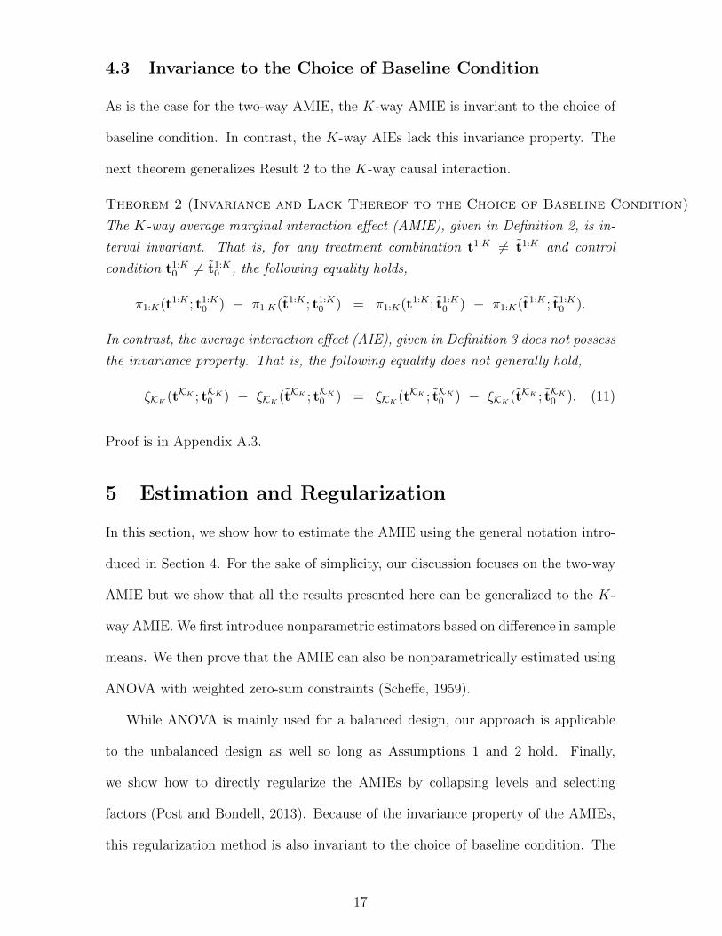
4.3 Invariance to the Choice of Baseline Condition
As is the case for the two-way AMIE, the K-way AMIE is invariant to the choice of
baseline condition. In contrast, the K-way AIEs lack this invariance property. The
next theorem generalizes Result 2 to the K-way causal interaction.
Theorem 2 (Invariance and Lack Thereof to the Choice of Baseline Condition)
The K-way average marginal interaction effect (AMIE), given in Definition 2, is in-
terval invariant. That is, for any treatment combination t1:K 6= t1:K and control
condition t1:K0 6= t1:K0 , the following equality holds,
π1:K(t1:K ; t1:K0 ) − π1:K(t1:K ; t1:K0 ) = π1:K(t1:K ; t1:K0 ) − π1:K(t1:K ; t1:K0 ).
In contrast, the average interaction effect (AIE), given in Definition 3 does not possess
the invariance property. That is, the following equality does not generally hold,
ξKK(tKK ; tKK
0 ) − ξKK(tKK ; tKK
0 ) = ξKK(tKK ; tKK
0 ) − ξKK(tKK ; tKK
0 ). (11)
Proof is in Appendix A.3.
5 Estimation and Regularization
In this section, we show how to estimate the AMIE using the general notation intro-
duced in Section 4. For the sake of simplicity, our discussion focuses on the two-way
AMIE but we show that all the results presented here can be generalized to the K-
way AMIE. We first introduce nonparametric estimators based on difference in sample
means. We then prove that the AMIE can also be nonparametrically estimated using
ANOVA with weighted zero-sum constraints (Scheffe, 1959).
While ANOVA is mainly used for a balanced design, our approach is applicable
to the unbalanced design as well so long as Assumptions 1 and 2 hold. Finally,
we show how to directly regularize the AMIEs by collapsing levels and selecting
factors (Post and Bondell, 2013). Because of the invariance property of the AMIEs,
this regularization method is also invariant to the choice of baseline condition. The
17

proposed method reduces false discovery and facilitates interpretation when there are
many factors and levels.
5.1 Difference-in-means Estimators
In the causal inference literature, the following difference-in-means estimators have
been used to nonparametrically estimate the ACE and AME (e.g., Hainmueller et al.,
2014; Dasgupta et al., 2015).
τjj′(`,m; 0, 0) =
∑ni=1 Yi1{Tij = `, Tij′ = m}∑ni=1 1{Tij = `, Tij′ = m}
−∑n
i=1 Yi1{Tij = 0, Tij′ = 0}∑ni=1 1{Tij = 0, Tij′ = 0}
,
ψj(`; 0) =
∑ni=1 Yi1{Tij = `}∑ni=1 1{Tij = `}
−∑n
i=1 Yi{Tij = 0}∑ni=1 1{Tij = 0}
.
These estimators are unbiased only when the treatment assignment distribution of
an experimental study is used to define the AMEs and AMIEs. Then, Definition 2
naturally implies the following nonparametric estimator of the two-way AMIE.
πjj′(`,m; 0, 0) = τjj′(`,m; 0, 0)− ψj(`; 0)− ψj′(m; 0).
Similarly, the nonparametric estimator of higher-order AMIE can be constructed. It
is important to emphasize that these nonparametric estimators do not assume the
absence of higher-order interactions (Hainmueller et al., 2014).
5.2 Nonparametric Estimation with ANOVA
Alternatively, the AMIEs can be estimated nonparametrically using ANOVA with
weighted zero-sum constraints, which is a convex optimization problem (Scheffe,
1959). For example, the two-way AMIE considered above can be estimated by the
saturated ANOVA whose objective function is as follows,
n∑i=1
Yi − µ− J∑j=1
Lj−1∑`=0
βj`1{Tij = `} −J−1∑j=1
∑j′>j
Lj−1∑`=0
Lj′−1∑m=0
βjj′
`m1{Tij = `, Tij′ = m}
−J∑k=3
∑Kk⊂KJ
∑tKk
βKk
tKk1{TKk
i = tKk}
)2
, (12)
18
where µ is the global mean, βj` is the coefficient for the first-order term for the jth
factor with ` level, βjj′
`m is the coefficient for the second-order interaction term for
the jth and j′th factors with ` and m levels, respectively, and more generally βKk
tKk
is the coefficient for the interaction term for a set of k factors Kk when their levels
equal to tKk . Note that as in Section 4, we have |Kk| = k and KJ = {1, 2, . . . , J}.
We emphasize that the nonparametric estimation requires all interaction terms up to
J-way interaction. See Section 5.3 for efficient parametric estimation.
We minimize the objective function given in equation (12) subject to the fol-
lowing weighted zero-sum constraints where the weights are given by the marginal
distribution of treatment assignment,
Lj−1∑`=0
Pr(Tij = `)βj` = 0 for all j, (13)
Lj−1∑`=0
Pr(Tij = `)βjj′
`m = 0 for all j 6= j′ and m ∈ {0, 1, . . . , Lj′ − 1}, (14)
Lj−1∑`=0
Pr(Tij = `)1{tj = `}βKk
tKk= 0 for all j, tKk , and Kk ⊂ KJ such that k ≥ 3 and j ∈ Kk.
(15)
Finally, the next theorem shows that the difference in the estimated ANOVA
coefficients represents a nonparametric estimate of the AMIE.
Theorem 3 (Nonparametric Estimation with ANOVA) Under Assumptions 1 and 2,
differences in the estimated coefficients from ANOVA based on equations (12)–(15)
represent nonparametric unbiased estimators of the AME and the AMIE:
E(βj` − βj0) = ψj(`; 0), E(βjj
′
`m − βjj′
00 ) = πjj′(`,m; 0, 0), E(βKk
tKk− βKk
tKk0
) = πKk(tKk ; tKk
0 ).
Proof is given in Appendix A.4. These estimators are asymptotically equivalent to
their corresponding difference-in-means estimators when the treatment assignment
distribution of an experimental study is used as weights. The proposed ANOVA
framework, however, allows researchers to use any treatment assignment distributions
to define the AME and the AMIE so long as Assumptions 1 and 2 hold.
19
5.3 Regularization
A key advantage of this ANOVA-based estimator in Section 5.2 over the difference-
in-means estimator in Section 5.1 is that we can directly regularize the AMIEs in a
penalized regression framework. The regularization is especially useful for reducing
false positives and facilitating interpretation when the number of factors is large.
We apply the regularization method (Grouping and Selection using Heredity in
ANOVA or GASH-ANOVA) proposed by Post and Bondell (2013), which places
penalties on difference in coefficients of the ANOVA regression. As shown above,
these differences correspond to the AMEs and AMIEs. While there exist other reg-
ularization methods for categorical variables (e.g., Yuan and Lin, 2006; Meier et al.,
2008; Zhao et al., 2009; Huang et al., 2009, 2012; Lim and Hastie, 2015), these meth-
ods regularize coefficients rather than their differences. In addition, GASH-ANOVA
collapses levels and selects factors by jointly considering the AMEs and AMIEs rather
than the AMEs alone. This is attractive because many social scientists believe large
interaction effects can exist even when marginal effects are small. The method also
collapses levels in a mutually consistent manner.
Finally, because the AMEs and AMIEs are invariant to the choice of baseline
condition, this regularization method also inherits the invariance property, which is
not generally the case (Lim and Hastie, 2015). In particular, even if one is interested
in conditional average causal effects, regularization should be based on the AMEs
and AMIEs because of their invariance property. As shown in equation (8), we can
compute the conditional average effects directly from these quantities.
To illustrate the application of GASH-ANOVA, consider a situation of practical
interest in which we assume the absence of causal interaction higher than the second
order. That is, in equation (12), we assume βKk
tKk= 0 for all k ≥ 3. GASH-ANOVA
collapses two levels within a factor by directly and jointly regularizing the AMEs and
20

AMIEs that involve those two levels. Define the set of all the AMEs and AMIEs that
involve levels ` and `′ of the jth factor as follows,
φj(`, `′) ={|βj` − β
j`′ |} ⋃ ⋃
j′ 6=j
Lj′−1⋃m=0
|βjj′
`m − βjj′
`′m|
.
Finally, the penalty is given by,
J∑j=1
∑`,`′
wj``′ max{φj(`, `′)} ≤ c,
where c is the cost parameter and wj``′ is the adaptive weight of the following form,
wj``′ =[(Lj + 1)
√Lj max{φj(`, `′)}
]−1,
where (Lj + 1)√Lj is the standardization factor (Bondell and Reich, 2009), and
φj(`, `′) represents the corresponding set of all AMEs and AMIEs estimated with-
out regularization. Post and Bondell (2013) show that, when combined with equa-
tions (12)–(15), the resulting optimization problem is a quadratic programming prob-
lem. They also prove that the method has the oracle property.
6 Empirical Analysis
We apply the proposed method to the conjoint analysis of coethnic voting described
in Section 2. Although conjoint analysis is based on the randomization of multiple
factors, it differs from factorial experiments in that respondents evaluate pairs of
randomly selected profiles. Thus, we only observe which profile they prefer within
a given pair but do not know how much they like each profile. As shown below,
this particular feature of conjoint analysis leads to a modified formulation of ANOVA
model. As explained in Section 5, we can apply the standard ANOVA (possibly
with regularization) to estimate the AMEs and AMIEs in a typical factorial experi-
ment. Our analysis finds clear patterns of causal interaction between the Record and
Coethnicity variables as well as between the Record and Platform variables.
21

6.1 A Statistical Model of Preference Differentials
Our empirical application is based on the choice-based conjoint analysis, in which
respondents are asked to evaluate three pairs of hypothetical presidential candidates
in turn. Let Yi(t) be the potential preference by respondent i for a hypothetical
candidate characterized by a vector of attributes t. In this experiment, t is a four
dimensional vector, based on the values of factorial treatments shown in Table 1 where
each factor Tij has Lj levels (i.e., {Coethnicity, Record, Platform, Degree}).
Given the limited sample size, we assume the absence of three-way or higher-
order causal interaction and use the following ANOVA regression model of potential
outcomes with all one-way effects and two-way interactions.
Yi(t) = µ+4∑j=1
Lj−1∑`=0
βj`1{tij = `}+4∑j=1
∑j′ 6=j
Lj−1∑`=0
Lj′−1∑m=0
βjj′
`m1{tij = `, tij′ = m}+ εi(t).
(16)
The results in Section 5.2 implies that the coefficients in this model represent the
AIEs and AMIEs.
In this conjoint analysis, respondents evaluate a pair of hypothetical candidates
with different attributes. This means that we only observe whether respondent i
prefers a candidate with attributes T∗i over another candidate with attributes T†i .
Thus, based on the model of preference given in equation (16), we construct a linear
probability model of preference differential,
Pr(Yi(T∗i ) > Yi(T
†i ) | T∗i ,T
†i )
= µ+4∑j=1
Lj−1∑`=0
βj` (1{T∗ij = `} − 1{T †ij = `})
+4∑j=1
∑j′ 6=j
Lj−1∑`=0
Lj′−1∑m=0
βjj′
`m(1{T ∗ij = `, T †ij′ = m} − 1{T ∗ij = `, T †ij′ = m}),
where µ = 0.5 if a position within a pair does not matter. Note that the independence
of irrelevant alternatives is assumed. If we additionally assume the difference in
22

errors follow independent Type I extreme value distributions, the model becomes the
conditional logit model, which is popular in conjoint analysis (McFadden, 1974).
We minimize the sum of squared residuals, subject to the constraints given in
equations (13) and (14) where Pr(Tij = `) represents the marginal distribution of T ∗ij
and T †ij together. We also apply the regularization method discussed in Section 5.3.
To be consistent with the original dummy coding, we treat Record and Platform as
ordered categorical variables and place penalties on the differences between adjacent
levels rather than the differences based on every pairwise comparison. We use the
order of levels as shown in Table 1. We choose the uniform distribution for treatment
assignment and select the value of the cost parameter c based on the minimum mean
squared error criterion in 10-fold cross validation.
Since the inference for a regularization method that collapses levels of factorial
variables is not established in the literature (Buhlmann and Dezeure, 2016), we focus
on the stability of selection (e.g., Breiman, 1996; Meinshausen and Buhlmann, 2010).
In particular, we estimate the selection probability for each AME and AMIE using
one minus the proportion of 5000 bootstrap replicates in which all coefficients for
the corresponding factor or factor interaction are estimated to be zero (Efron, 2014;
Hastie et al., 2015). Although we do not control the family wise error rate, we follow
Meinshausen and Buhlmann (2010) and use 90% cutoff as our default.
Another possible inferential approach is sample splitting where we collapse lev-
els and select factors using training data and then estimate and compute confidence
intervals for the AMEs and AMIEs using test data (Athey and Imbens, 2016; Cher-
nozhukov et al., 2017; Wasserman and Roeder, 2009). Although we do not present the
results based on this approach here, it can be implemented through our open-source
software package, FindIt.
23

SelectionRange prob.
AMERecord 0.122 1.00Coethnicity 0.053 1.00Platform 0.023 1.00Degree 0.000 0.58
AMIECoethnicity × Record 0.054 1.00Record × Platform 0.030 1.00Platform × Coethnicity 0.008 0.99Record × Degree 0.000 0.60Coethnicity × Degree 0.000 0.60Platform × Degree 0.000 0.60
Table 2: Ranges of the Estimated Average Marginal Effects (AMEs) and EstimatedAverage Marginal Interaction Effects (AMIEs). The estimated selection probabilityof the AME (AMIE) is one minus the proportion of 5000 bootstrap replicates in whichall coefficients for the corresponding factor (factor interaction) are estimated to bezero.
6.2 Findings
We begin by reporting the ranges of the estimated AMEs and AMIEs and their selec-
tion probability to determine significant factors and factor interactions, respectively.
As shown in Table 2, three factors — Record, Platform, and Coethnicity — are
found to be significant factors whereas Degree is not. In terms of the AMIEs, the
interaction Coethnicity × Record, which is the basis of the main finding in the
original article, is estimated to have a large range of 5.4 percentage point, and is
selected with probability one. The range of this AMIE is as great as that of the
AME of Coethnicity and is greater than that of Platform. Additionally, the pro-
posed method selects the causal interactions, Record × Platform and Platform ×
Coethnicity, with probability close to one. We focus on the two largest causal
interactions, Coethnicity × Record and Record × Platform.
Next, we examine the estimated AMEs presented in Table 3. For the Record
variable, under the 90% selection probability rule, we collapse a total of original
24

SelectionFactor AME prob.Record
Yes/VillageYes/DistrictYes/MPNo/VillageNo/DistrictNo/MP
{ No/Businessman
0.1220.1220.1010.0470.0510.047base
〉 0.64〉 0.80〉 1.00〉 0.76〉 0.84〉 0.99
Platform{JobsClinic
{ Education
−0.023−0.023
base
〉 0.80〉 0.97
Coethnicity 0.053 1.00Degree 0.000 0.57
Table 3: The Estimated Average Marginal Effects (AMEs). The estimated selectionprobability is the proportion of 5000 bootstrap replicates in which the differencebetween two adjacent levels is estimated to be different from zero.
seven levels into three levels – {Yes/Village, Yes/District, Yes/MP}, {No/Village,
No/District , No/MP}, and {No/Businessman}. This partition suggests that politi-
cians with good record are preferred over those without it including businessman.
Similarly, we find two groups in the Platform variable – {Jobs, Clinic} and {Education}
– where voters appear to favor candidates with the education platform on average.
We now investigate two significant causal interactions, Coethnicity × Record
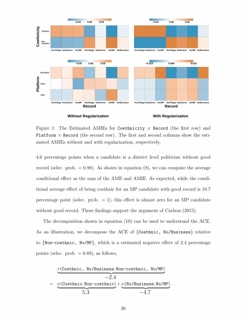
and Record × Platform. Figure 1 visualizes all estimated AMIEs within each fac-
tor interaction. The cells with warmer red (colder blue) color represents a greater
(smaller) AMIE than the average AMIE within that factor interaction. The estimates
with regularization (right column) show clearer patterns for causal interaction than
those without regularization (left column).
First, regarding the Coethnicity × Record interaction (upper panel of the fig-
ure), for example, we find that being coethnic gives an average bonus of 5.3 percentage
point if a candidate is an MP with good record beyond the average effect of coeth-
nicity (selec. prob. = 1). In contrast, being coethnic has an additional penalty of
25
NonCoethnic
Coethnic
Yes/Village Yes/District Yes/MP No/Village No/District No/MP No/Business
−0.04 0.00 0.04
Jobs
Clinic
Education
Yes/Village Yes/District Yes/MP No/Village No/District No/MP No/Business
Record
−0.05 0.00 0.05
Without Regularization
Yes/Village Yes/District Yes/MP No/Village No/District No/MP No/Business
−0.02 0.00 0.02
Yes/Village Yes/District Yes/MP No/Village No/District No/MP No/Business
Record
−0.015 0.000 0.015
With Regularization
Coe
thni
city
Pla
tform
Figure 1: The Estimated AMIEs for Coethnicity × Record (the first row) and
Platform × Record (the second row). The first and second columns show the esti-
mated AMIEs without and with regularization, respectively.
4.6 percentage points when a candidate is a district level politician without good
record (selec. prob. = 0.98). As shown in equation (8), we can compute the average
conditional effect as the sum of the AME and AMIE. As expected, while the condi-
tional average effect of being coethnic for an MP candidate with good record is 10.7
percentage point (selec. prob. = 1), this effect is almost zero for an MP candidate
without good record. These findings support the argument of Carlson (2015).
The decomposition shown in equation (10) can be used to understand the ACE.
As an illustration, we decompose the ACE of {Coethnic, No/Business} relative
to {Non-coethnic, No/MP}, which is a estimated negative effect of 2.4 percentage
points (selec. prob. = 0.89), as follows,
τ(Coethnic, No/Business; Non-coethnic, No/MP)︸ ︷︷ ︸−2.4
= ψ(Coethnic; Non-coethnic)︸ ︷︷ ︸5.3
+ψ(No/Business; No/MP)︸ ︷︷ ︸−4.7
26

+ π(Coethnic, No/Business; Non-coethnic, No/MP)︸ ︷︷ ︸−3.0
.
We observe that while the average effect of being coethnic is 5.3 percentage points,
being a businessman, relative to being an MP without good record, yields an average
effect of negative 4.7 percentage points. In addition, being a coethnic businessman
has an additional penalty of 3 percentage points relative to non-coethnic MP without
good record. All three estimates are selected with probability close to one.
Finally, we examine the Platform × Record interaction, which was not discussed
in the original study. We find two distinct groups: (1) politicians with record, busi-
nessmen without record and (2) politicians without record. Candidates in the second
group appear to receive an additional penalty by promising to improve education.
Specifically, the estimated AMIE of {Education, No/MP} relative to {Job, No/MP}
is −2.3 percentage point (selec. prob. = 0.99). In fact, the average conditional effect
of Education relative to Job given No/MP is about zero (selec. prob. = 0.75). These
results suggest that even though promising to improve education is effective on aver-
age (the estimated AME of Education relative to Job is 2.3 percentage point (selec.
prob. = 0.98), it has no effect for politicians without record.
7 Concluding Remarks
In this paper, we propose a new causal interaction effect for randomized experiments
with a factorial design, in which there exist many factors with each having several
levels. We call this quantity, the average marginal interaction effect (AMIE). Unlike
the conventional causal interaction effect, the AMIE is invariant to the choice of base-
line. This enables us to provide a simpler interpretation even in a high-dimensional
setting. We show how to nonparametrically estimate the AMIE within the ANOVA
regression framework. The invariance property also enables us to apply a regular-
ization method by directly penalizing the AMIEs. This reduces false discovery and
27
facilitates interpretation.
We emphasize that the AMIE, which is a generalization of the average marginal
effect studied in the literature on factorial experiments, critically depends on the dis-
tribution of treatments. For example, in a well-known audit study of labor market
discrimination where researchers randomize the information on the resume of a fic-
titious job applicant (e.g., Bertrand and Mullainathan, 2004), the average effect of
applicant’s race requires the specification of other attributes such as education levels
and prior job experiences. In the real world, these characteristics may be correlated
with race and act as an effect modifier. Thus, ideally, researchers should obtain the
target population distribution of treatments, e.g., the characteristics of job applicants
in a relevant labor market, and use it as the basis for treatment randomization. This
will improve the external validity of experimental studies.
Finally, our method is motivated by and applied to conjoint analysis, a popular
survey experiment with a factorial design. The methodological literature on conjoint
analysis has largely ignored the role of causal interaction. The method proposed in
this paper allows researchers to effectively explore significant causal interaction among
several factors. Although not investigated in this paper, future research should in-
vestigate interaction between treatments and pre-treatment covariates. It is also of
interest to develop sequential experimental designs in the context of factorial experi-
ments so that researchers can efficiently reduce the number of treatments.
28

References
Athey, S. and Imbens, G. (2016). Recursive partitioning for heterogeneous causal
effects. Proceedings of the National Academy of Sciences 113, 27, 7353–7360.
Bertrand, M. and Mullainathan, S. (2004). Are Emily and Greg more employable than
Lakisha and Jamal?: A field experiment on labor market discrimination. American
Economic Review 94, 4, 991–1013.
Bondell, H. D. and Reich, B. J. (2009). Simultaneous factor selection and collapsing
levels in anova. Biometrics 65, 1, 169–177.
Breiman, L. (1996). Heuristics of instability and stabilization in model selection. The
Annals of Statistics 24, 6, 2350–2383.
Buhlmann, P. and Dezeure, R. (2016). Discussion of ‘regularized regression for cate-
gorical data’ by tutz and gertheiss. Statistical Modelling 16, 3, 205–211.
Carlson, E. (2015). Ethnic voting and accountability in africa: A choice experiment
in uganda. World Politics 67, 02, 353–385.
Chernozhukov, V., Chetverikov, D., Demirer, M., Duflo, E., Hansen, C., Newey,
W., and Robins, J. (2017). Double/debiased machine learning for treatment and
structural parameters. arXiv preprint arXiv:1608.00060 .
Cox, D. R. (1958). Planning of Experiments. John Wiley & Sons, New York.
Cox, D. R. (1984). Interaction. International Statistical Review 52, 1, 1–24.
Dasgupta, T., Pillai, N. S., and Rubin, D. B. (2015). Causal inference from 2k factorial
designs by using potential outcomes. Journal of the Royal Statistical Society, Series
B (Statistical Methodology) 77, 4, 727–753.
29

de Gonzalez, A. B. and Cox, D. R. (2007). Interpretation of interaction: A review.
The Annals of Applied Statistics 1, 2, 371–385.
Efron, B. (2014). Estimation and accuracy after model selection. Journal of the
American Statistical Association 109, 507, 991–1007.
Egami, N., Ratkovic, M., and Imai, K. (2017). FindIt: Finding heterogeneous
treatment effects. available at the Comprehensive R Archive Network (CRAN).
https://CRAN.R-project.org/package=FindIt.
Green, D. P. and Kern, H. L. (2012). Modeling heterogeneous treatment effects in
survey experiments with bayesian additive regression trees. Public opinion quarterly
76, 3, 491–511.
Green, P. E., Krieger, A. M., and Wind, Y. (2001). Thirty years of conjoint analysis:
Reflections and prospects. Interfaces 31, 3 supplement, 56–73.
Green, P. E. and Rao, V. R. (1971). Conjoint measurement for quantifying judgmental
data. Journal of Marketing research 355–363.
Grimmer, J., Messing, S., and Westwood, S. J. (2017). Estimating heterogeneous
treatment eects andthe eects of heterogeneous treatments with ensemble methods.
Political Analysis 25, 413–434.
Hainmueller, J. and Hopkins, D. J. (2015). The hidden american immigration con-
sensus: A conjoint analysis of attitudes toward immigrants. American Journal of
Political Science 59, 3, 529–548.
Hainmueller, J., Hopkins, D. J., and Yamamoto, T. (2014). Causal inference in
conjoint analysis: Understanding multidimensional choices via stated preference
experiments. Political Analysis 22, 1, 1–30.
30

Hastie, T., Tibshirani, R., and Wainwright, M. (2015). Statistical learning with spar-
sity: the lasso and generalizations. CRC Press.
Hill, J. L. (2012). Bayesian nonparametric modeling for causal inference. Journal of
Computational and Graphical Statistics 20, 1, 217–240.
Huang, J., Breheny, P., and Ma, S. (2012). A selective review of group selection in
high-dimensional models. Statistical Science 27, 4, 481–499.
Huang, J., Ma, S., Xie, H., and Zhang, C.-H. (2009). A group bridge approach for
variable selection. Biometrika 96, 2, 339–355.
Imai, K. and Ratkovic, M. (2013). Estimating treatment effect heterogeneity in
randomized program evaluation. Annals of Applied Statistics 7, 1, 443–470.
Jaccard, J. and Turrisi, R. (2003). Interaction effects in multiple regression. Sage
Publications.
Lim, M. and Hastie, T. (2015). Learning interactions via hierarchical group-lasso
regularization. Journal of Computational and Graphical Statistics 24, 3, 627–654.
Lu, J. (2016a). Covariate adjustment in randomization-based causal inference for 2k
factorial designs. Statistics & Probability Letters 119, 11–20.
Lu, J. (2016b). On randomization-based and regression-based inferences for 2k fac-
torial designs. Statistics & Probability Letters 112, 72–78.
Luce, R. D. and Tukey, J. W. (1964). Simultaneous conjoint measurement: A new
type of fundamental measurement. Journal of mathematical psychology 1, 1, 1–27.
Marshall, D., Bridges, J. F., Hauber, B., Cameron, R., Donnalley, L., Fyie, K., and
Johnson, F. R. (2010). Conjoint analysis applications in health: How are studies
31

being designed and reported? The Patient: Patient-Centered Outcomes Research
3, 4, 249–256.
Marshall, P. and Bradlow, E. T. (2002). A unified approach to conjoint analysis
models. Journal of the American Statistical Association 97, 459, 674–682.
McFadden, D. (1974). Conditional logit analysis of qualitative choice behavior. In
P. Zarembka, ed., Frontiers in econometrics. Academic Press.
Meier, L., Van De Geer, S., and Buhlmann, P. (2008). The group lasso for logistic re-
gression. Journal of the Royal Statistical Society: Series B (Statistical Methodology)
70, 1, 53–71.
Meinshausen, N. and Buhlmann, P. (2010). Stability selection. Journal of the Royal
Statistical Society: Series B (Statistical Methodology) 72, 4, 417–473.
Murphy, S. A. (2003). Optimal dynamic treatment regimes (with discussions). Journal
of the Royal Statistical Society, Series B (Statistical Methodology) 65, 2, 331–366.
Post, J. B. and Bondell, H. D. (2013). Factor selection and structural identification
in the interaction anova model. Biometrics 69, 1, 70–79.
Robins, J. M. (2004). Optimal structural nested models for optimal sequential deci-
sions. In Proceedings of the Second Seattle Symposium in Biostatistics: Analysis of
Correlated Data (eds., D. Y. Lin and P. J. Heagerty, New York. Springer.
Rubin, D. B. (1990). Comments on “On the application of probability theory to
agricultural experiments. Essay on principles. Section 9” by J. Splawa-Neyman
translated from the Polish and edited by D. M. Dabrowska and T. P. Speed. Sta-
tistical Science 5, 472–480.
Scheffe, H. (1959). The analysis of variance. John Wiley & Sons.
32
VanderWeele, T. (2015). Explanation in causal inference: methods for mediation and
interaction. Oxford University Press.
VanderWeele, T. J. and Knol, M. J. (2014). A tutorial on interaction. Epidemiologic
Methods Epidemiol. Methods 3, 1, 33–72.
Wager, S. and Athey, S. (2017). Estimation and inference of heterogeneous treat-
ment effects using random forests. Journal of the American Statistical Association
Forthcoming.
Wasserman, L. and Roeder, K. (2009). High dimensional variable selection. Annals
of statistics 37, 5A, 2178.
Wu, C. J. and Hamada, M. S. (2011). Experiments: planning, analysis, and opti-
mization, vol. 552. John Wiley & Sons.
Yuan, M. and Lin, Y. (2006). Model selection and estimation in regression with
grouped variables. Journal of the Royal Statistical Society: Series B (Statistical
Methodology) 68, 1, 49–67.
Zhao, P., Rocha, G., and Yu, B. (2009). The composite absolute penalties family
for grouped and hierarchical variable selection. The Annals of Statistics 37, 6A,
3468–3497.
33

A Mathematical Appendix: Proofs of Theorems
A.1 Lemmas
Below, we describe all the lemmas, which are used to prove the main theorems of this
paper. For completeness, their proofs appear in the supplementary appendix.
Lemma 1 (An Alternative Definition of the K-way Average Interaction Effect)
The K-way average interaction effect (AIE) of treatment combination T1:Ki = t1:K =
(t1, . . . , tK) relative to baseline condition T1:Ki = t1:K0 = (t01, . . . , t0K), given in Defi-
nition 3, can be rewritten as,
ξ1:K(t1:K ; t1:K0 ) = ξ1:(K−1)(t1:(K−1); t
1:(K−1)0 | TiK = tK)− ξ1:(K−1)(t1:(K−1); t1:(K−1)0 | TiK = t0K).
Lemma 2 Under Assumption 2, for any k = 1, . . . , K, the following equality holds,∫FKk
ξKK(TKk , tKK\Kk ; tKK
0 )dF (TKk) = ξKK\Kk(tKK\Kk , t
KK\Kk
0 )
+k∑`=1
(−1)`∑K`⊆Kk
∫FKk\K`
ξKK\Kk(tKK\Kk , t
KK\Kk
0 | TKk\K` ,TK`
i = tK`0 )dF (TKk\K`).
Lemma 3 (Decomposition of the K-way AIE) The K-way Average Treatment
Interaction Effect (AIE) (Definition 3), can be decomposed into the sum of the K-
way conditional Average Treatment Combination Effects (ACEs). Formally, let Kk ⊆KK = {1, . . . , K} with |Kk| = k where k = 1, . . . , K. Then, the K-way AIE can be
written as follows,
ξKK(tKK ; tKK
0 ) =K∑k=1
(−1)K−k∑Kk⊆KK
τKk(tKk ; tKk
0 | TKK\Kk
i = tKK\Kk
0 ),
where the second summation is taken over the set of all possible Kk and the k-way
conditional ACE is defined as,
τKk(tKk ; tKk
0 | TKK\Kk
i = tKK\Kk
0 ) = E[∫FKK
{Yi(tKk , tKK\Kk
0 , TiKK )− Yi(tKk
0 , tKK\Kk
0 , TiKK )}dF (TKK
i )
].
Lemma 4 (Decomposition of the K-way AMIE) The K-way Average Marginal
Treatment Interaction Effect (AMIE), defined in Definition 2, can be decomposed into
the sum of the K-way Average Treatment Combination Effects (ACEs). Formally, let
34
Kk ⊆ KK = {1, . . . , K} with |Kk| = k where k = 1, . . . , K. Then, the K-way AMIE
can be written as follows,
πKK(tKK ; tKK
0 ) =K∑k=1
(−1)K−k∑Kk⊆KK
τKk(tKk ; tKk
0 ),
where the second summation is taken over the set of all possible Kk.
A.2 Proof of Theorem 1
We use proof by induction. Under Assumption 2, we first show for K = 2. To simplify
the notation, we do not write out the J−2 factors that we marginalize out. We begin
by decomposing the AME as follows,
ψA(al, a0) =
∫BE{Yi(a`, Bi)− Yi(a0, Bi)} dF (Bi)
= E{Yi(a`, b0)− Yi(a0, b0)}+
∫BE{Yi(a`, Bi)− Yi(a0, Bi)− Yi(a`, b0) + Yi(a0, b0)} dF (Bi)
= E{Yi(a`, b0)− Yi(a0, b0)}+
∫BξAB(a`, Bi; a0, b0) dF (Bi).
Similarly, we have ψB(bm, b0) = E{Yi(a0, bm)−Yi(a0, b0)}+∫A ξAB(Ai, bm; a0, b0) dF (Ai).
Given the definition of the AMIE in equation (5), we have,
πAB(a`, bm, a0, b0) = E{Yi(a`, bm)− Yi(a0, b0)} − ψA(a`, a0)− ψB(bm, b0)
= ξAB(a`, bm; a0, b0)−∫BξAB(a`, Bi; a0, b0) dF (Bi)−
∫AξAB(Ai, bm; a0, b0) dF (Ai).
This proves that the AMIE is a linear function of the AIEs. We next show that the
AIE is also a linear function of the AMIEs.
ξAB(a`, bm; a0, b0) = E{Yi(a`, bm)− Yi(a0, b0)} − ψA(a`, a0)− ψA(bm, b0)
− E{Yi(a`, b0)− Yi(a0, b0)}+ ψA(a`, a0)− E{Yi(a0, bm)− Yi(a0, b0)}+ ψA(bm, b0)
= πAB(a`, bm; a0, b0)− πAB(a`, b0; a0, b0)− πAB(a0, bm; a0, b0).
Thus, we obtain the desired results for K = 2.
35

Now we show that if the theorem holds for any K with K ≥ 2, it also holds for
K + 1. First, using Lemma 2, we rewrite the equation of interest as follows,
πKK(tKK ; tKK
0 ) = ξKK(tKK ; tKK
0 ) +K−1∑k=1
(−1)k∑Kk⊆KK
{ξKK\Kk
(tKK\Kk , tKK\Kk
0 )
+k∑`=1
(−1)`∑K`⊆Kk
∫FKk\K`
ξKK\Kk(tKK\Kk , t
KK\Kk
0 | TKk\K` ,TK`
i = tK`0 )dF (TKk\K`)
}.
Utilizing the the definition of the K-way AMIE given in Definition 2 and the assump-
tion that the theorem holds for K, we have,
πKK+1(tKK+1 ; t
KK+1
0 ) = τKK+1(tKK+1 ; t
KK+1
0 )−K∑k=1
∑Kk⊆KK+1
πKk(tKk ; tKk
0 )
= τKK+1(tKK+1 ; t
KK+1
0 )
−K∑k=1
∑Kk⊆KK+1
[ξKk
(tKk ; tKk0 ) +
k−1∑m=1
(−1)m∑Km⊆Kk
{ξKk\Km(tKk\Km , t
Kk\Km
0 )
+m∑`=1
(−1)`∑K`⊆Km
∫FKm\K`
ξKk\Km(tKk\Km , tKk\Km
0 | TKm\K` ,TK`
i = tK`0 )dF (TKm\K`)
}].
(17)
After rearranging equation (17), the coefficient for ξKK+1\Ku(tKK+1\Ku , tKK+1\Ku
0 )
is equal to (−1)u. Similarly, the coefficient of the following term is equal to (−1)u+v.∫FKu\Kv
ξKK+1\Ku(tKK+1\Ku , tKK+1\Ku
0 | TKu\Kv ,TKv
i = tKv0 )dF (TKu\Kv).
Therefore, we can rewrite equation (17) as follows,
πKK+1(tKK+1 ; t
KK+1
0 )
= τKK+1(tKK+1 ; t
KK+1
0 ) +K∑k=1
(−1)k∑
Kk⊆KK+1
{ξKK+1\Kk
(tKK+1\Kk , tKK+1\Kk
0 )
+k−1∑`=1
(−1)`∑K`⊆Kk
∫FKk\K`
ξKK+1\Kk(tKK+1\Kk , t
KK+1\Kk
0 | TKk\K` ,TK`
i = tK`0 )dF (TKk\K`)
}
= ξKK+1(tKK+1 ; t
KK+1
0 ) +K∑k=1
(−1)k∑
Kk⊆KK+1
{ξKK+1\Kk
(tKK+1\Kk , tKK+1\Kk
0 )
+k∑`=1
(−1)`∑K`⊆Kk
∫FKk\K`
ξKK+1\Kk(tKK+1\Kk , t
KK+1\Kk
0 | TKk\K` ,TK`
i = tK`0 )dF (TKk\K`)
}
36

= ξKK+1(tKK+1 ; t
KK+1
0 ) +K∑k=1
(−1)k∑
Kk⊆KK+1
∫ξ(TKk , tKK+1\Kk ; t
KK+1
0 )dF (TKk),
where the second equality follows from applying Lemma 1 to τKK+1(tKK+1 ; t
KK+1
0 ) and
the final equality from Lemma 2. This proves that the K-way AMIE is a linear
function of the K-way AIEs.
We next prove that the K-way AIE can be written as a linear function of the
K-way AMIEs. We will show this by mathematical induction. We already show the
desired result holds for K = 2. Choose any K ≥ 2 and assume that the following
equality holds,
ξKK(tKK ; tKK
0 ) =K∑k=1
(−1)K−k∑Kk⊆KK
πKK(tKk , t
KK\Kk
0 ; tKk0 , t
KK\Kk
0 ).
Using the definition of the K-way AIE given in Lemma 1, we have
ξKK+1(tKK+1 ; t
KK+1
0 ) = ξKK(tKK ; tKK
0 | TK+1i = tK+1)− ξKK
(tKK ; tKK0 | TK+1
i = tK+10 )
=K∑k=1
(−1)K−k∑Kk⊆KK
πKK+1(tKk , t
KK\Kk
0 , tK+1; tKk0 , t
KK\Kk
0 , tK+1)
−K∑k=1
(−1)K−k∑Kk⊆KK
πKK+1(tKk , t
KK\Kk
0 , tK+10 ; tKk
0 , tKK\Kk
0 , tK+10 ),
where the second equality follows from the assumption. Let us consider the following
decomposition.
K+1∑k=1
(−1)K−k+1∑
Kk⊆KK+1
πKK+1(tKk , t
KK+1\Kk
0 ; tKk0 , t
KK+1\Kk
0 )
=K∑k=1
(−1)K−k∑Kk⊆KK
πKK+1(tKk , t
KK\Kk
0 , tK+1; tKk0 , t
KK\Kk
0 , tK+10 ) + (−1)KπKK+1
(tKK0 , tK+1; tKK
0 , tK+10 )
+K∑k=1
(−1)K−k+1∑Kk⊆KK
πKK+1(tKk , t
KK\Kk
0 , tK+10 ; tKk
0 , tKK\Kk
0 , tK+10 ), (18)
where the first and second terms together represent the cases with K + 1 ∈ Kk, while
the third term corresponds to the cases with K + 1 ∈ KK+1 \ Kk. Note that these
two cases are mutually exclusive and exhaustive. Finally, note the following equality,
K∑k=1
(−1)K−k∑Kk⊆KK
πKK+1(tKk , t
KK\Kk
0 , tK+1; tKk0 , t
KK\Kk
0 , tK+1)
37

=K∑k=1
(−1)K−k∑Kk⊆KK
πKK+1(tKk , t
KK\Kk
0 , tK+1; tKk0 , t
KK\Kk
0 , tK+10 ) + (−1)KπKK+1
(tKK0 , tK+1; tKK
0 , tK+10 ).
(19)
Then, together with equations (18) and (19), we obtain,
ξKK+1(tKK+1 ; t
KK+1
0 ) =K+1∑k=1
(−1)K−k+1∑
Kk⊆KK+1
πKK+1(tKk , t
KK+1\Kk
0 ; tKk0 , t
KK+1\Kk
0 ).
Thus, the desired linear relationship holds for any K ≥ 2. 2
A.3 Proof of Theorem 2
To prove the invariance of the K-way AMIE, note that Lemma 4 implies,
πKK(t; t0) − πKK
(t; t0) =K∑k=1
(−1)K−k∑Kk⊆KK
τKk(tKk ; tKk). (20)
πKK(t; t0) − πKK
(t; t0) =K∑k=1
(−1)K−k∑Kk⊆KK
τKk(tKk ; tKk). (21)
Thus, the K-way AMIE is interval invariant. To prove the lack of invariance of the
K-way AIE, note that according to Lemma 3, we can rewrite equation (11) as follows.
K∑k=1
(−1)K−k∑Kk⊆KK
{τKk
(tKk ; tKk0 | T
KK\Kk
i = tKK\Kk
0 )− τKk(tKk ; tKk
0 | TKK\Kk
i = tKK\Kk
0 )
}
=K∑k=1
(−1)K−k∑Kk⊆KK
{τKk
(tKk ; tKk0 | T
KK\Kk
i = tKK\Kk
0 )− τKk(tKk ; tKk
0 | TKK\Kk
i = tKK\Kk
0 )
}.
It is clear that this equality does not hold in general because the K-way conditional
ACEs are conditioned on different treatment values. Thus, the K-way AIE is not
interval invariant. 2
A.4 Proof of Theorem 3
We use L to denote the objective function in equation (12). Since it is a convex
optimization problem, it has one unique solution and the solution should satisfy the
following equalities.
∂L
∂µ= 0,
∂L
∂βj`= 0 for all j, and ` ∈ {0, 1, . . . , Lj − 1},
38

∂L
∂βjj′
`,m
= 0, for all j 6= j′, ` ∈ {0, 1, . . . , Lj − 1} and m ∈ {0, 1, . . . , Lj′ − 1},
∂L
∂βKk
tKk
= 0 for all tKk , and Kk ⊂ KJ such that k ≥ 3. (22)
For the sake of simplicity, we introduce the following notation.
S(tKk) ≡ {i; TKki = tKk}, NtKk ≡
n∑i=1
1{TKki = tKk}, E[Yi | TKk
i = tKk ] ≡ 1
NtKk
∑i∈S(tKk )
Yi.
Then, from ∂L
∂βββKJ
tKJ
= 0 for all tKJ ,
∂L
∂βββKJ
tKJ
=∑
i∈S(tKk )
−2
(Yi − µ−
J∑j=1
Lj−1∑`=0
βj`1{Tij = `} −J−1∑j=1
∑j′>j
Lj−1∑`=0
Lj′−1∑m=0
βjj′
`m1{Tij = `, Tij′ = m}
−J∑k=3
∑Kk⊂KJ
∑tKk
βKk
tKk1{TKk
i = tKk})
= 0. (23)
Therefore, for all tKJ ,
µ+J∑k=1
∑Kk⊂KJ
∑tKk
βKk
tKk1{tKk ⊂ tKJ} = E[Yi | TKJ
i = tKJ ].
For the first-order effect, we can use the weighted zero-sum constraints for all
factors except for the j th factor. In particular, for all j and tj` ∈ tKJ ,
∑j′ 6=j
Lj′−1∑`=0
∏tj′`∈tKJ\j
Pr(Tij′ = `)
{µ+
J∑k=1
∑Kk⊂KJ
∑tKk
βKk
tKk1{tKk ∈ tKJ}
}
=∑j′ 6=j
Lj′−1∑`=0
∏tj′`∈tKJ\j
Pr(Tij′ = `) E[Yi | Tij = `,TKJ\ji = tKJ\j]
⇐⇒ βj` =∑j′ 6=j
Lj′−1∑`=0
∏tj′`∈tKJ\j
Pr(Tij′ = `) E[Yi | Tij = `,TKJ\ji = tKJ\j]− µ.
In general, for all tKk ,Kk ⊂ KJ and k ≥ 2,
βKk
tKk=
∑j′∈KJ\Kk
Lj′−1∑`=0
∏tj′`∈tKJ\Kk
Pr(Tij′ = `) E[Yi | TKki = tKk ,T
KJ\Kk
i = tKJ\Kk ]
−∑Kp⊂Kk
∑tKp
1{tKp ⊂ tKk}βKp
tKp − µ. (24)
In addition, µ is given as follows.
µ =K∑j=1
Lj−1∑`=0
∏tj`∈tKJ
Pr(Tij = `) E[Yi | TKJi = tKJ ].
39

Therefore, (µ, βββ) is uniquely determined. To confirm this solution is the minimizer
of the optimization problem, we check all the equality conditions. For all tKk ,Kk ⊂
KJ , j ∈ Kk and k ≥ 1,
Lj−1∑`=0
Pr(Tij = `)1{tj = `}βKk
tKk
=
Lj−1∑`=0
Pr(Tij = `)1{tj = `}∑
j′∈KJ\Kk
Lj′−1∑`=0
∏tj′`∈tKJ\Kk
Pr(Tij′ = `) E[Yi | TKki = tKk ,T
KJ\Kk
i = tKJ\Kk ]
−Lj−1∑`=0
Pr(Tij = `)1{tj = `}∑Kp⊂Kk
∑tKp
1{tKp ⊂ tKk}βKp
tKp − µ
=∑
j′∈{j,KJ\Kk}
Lj′−1∑`=0
∏tj′`∈t{j,KJ\Kk}
Pr(Tij′ = `) E[Yi | TKk\ji = tKk\j,T
{j,KJ\Kk}i = t{j,KJ\Kk}]
−∑
Kp⊆Kk\j
∑tKp
1{tKp ⊆ tKk\j}βKp
tKp − µ
= 0,
where the final equality comes from equation (24) for βKk\jtKk\j .
Furthermore, equation (23) implies all other equalities in equation (22). Therefore,
the solution (equations (24) and (25)) satisfies all the equality conditions. Finally,
we show that these estimators are unbiased for the AMEs and the AMIEs. Since
E[Yi | TKJi = tKJ ] is an unbiased estimator of E[Yi(t
KJ )],
E(βKk
tKk) =
∑j′∈KJ\Kk
Lj′−1∑`=0
∏tj′`∈tKJ\Kk
Pr(Tij′ = `) E[Yi(tKk , tKJ\Kk)]
−∑Kp⊂Kk
∑tKp
1{tKp ⊂ tKk}E[βKp
tKp ]− µ,
E(βKk
tKk− βKk
tKk0
) =∑
j′∈KJ\Kk
Lj′−1∑`=0
∏tj′`∈tKJ\Kk
Pr(Tij′ = `) E[Yi(tKk , tKJ\Kk)− Yi(tKk
0 , tKJ\Kk)]
−∑Kp⊂Kk
∑tKp
1{tKp ⊂ tKk}E[βKp
tKp − βKp
tKp0
]
= πKk(tKk ; tKk
0 ).
2
40

B Supplementary Appendix: Proofs of Lemmas
For the sake of completeness, we prove all the lemmas used in the mathematical
appendix above.
B.1 Proof of Lemma 1
To simplify the proof, we start from Lemma 1 and prove it is equivalent to Definition 3.
We prove it by induction. Equation (7) shows this correspondence holds for K = 2.
Next, choose any K ≥ 2 and assume that this relationship holds. That is, we assume
the following equality,
ξKK(t; t0) = τKK
(t; t0) −K−1∑k=1
∑Kk⊆KK
ξKk(tKk ; tKk
0 | TKK\Kk
i = tKK\Kk
0 ), (25)
where the second summation is taken over all possible Kk ⊆ KK = {1, . . . , K} with
|Kk| = k.
Using the definition of the K-way AIE in Lemma 1, we have,
K−1∑k=1
∑Kk⊆KK
ξ{Kk,K+1}(tKk , tK+1; t
Kk0 , t0,K+1 | T
KK\Kk
i = tKK\Kk
0 )
=K−1∑k=1
∑Kk⊆KK
ξKk(tKk ; tKk
0 | Ti,K+1 = tK+1,TKK\Kk
i = tKK\Kk
0 )
−K−1∑k=1
∑Kk⊆KK
ξKk(tKk ; tKk
0 | Ti,K+1 = t0,K+1,TKK\Kk
i = tKK\Kk
0 ), (26)
where ξ{Kk,K+1}(tKk , tK+1; t
Kk0 , t0,K+1 | T
KK\Kk
i = tKK\Kk
0 ) denote the conditional (k+
1)-way AIE that includes the set of k treatments, Kk, as well as the (K + 1)th
treatment while fixing TKK\Kk
i to tKK\Kk
0 . Therefore, we have,
ξKK+1(tKK+1 ; t
KK+1
0 )
= ξKK(tKK ; tKK
0 | Ti,K+1 = tK+1)− ξKK(tKK ; tKK
0 | Ti,K+1 = t0,K+1)
= τKK+1(tKK , tK+1; t
KK0 , tK+1)− τKK+1
(tKK , t0,K+1; tKK0 , t0,K+1)
41
−K−1∑k=1
∑Kk⊆KK
ξ{Kk,K+1}(tKk , tK+1; t
Kk0 , t0,K+1 | T
KK\Kk
i = tKK\Kk
0 )
= τKK+1(tKK , tK+1; t
KK0 , tK+1)−
K∑k=1
∑Kk⊆KK
ξKk(tKk ; tKk
0 | TKK+1\Kk
i = tKK+1\Kk
0 )
−K−1∑k=1
∑Kk⊆KK
ξ{Kk,K+1}(tKk , tK+1; t
Kk0 , t0,K+1 | T
KK\Kk
i = tKK\Kk
0 ), (27)
where the second equality follows from equation (26), and the third equality is based
on the application of the assumption given in equation (25) while conditioning on
Ti,K+1 = t0,K+1.
Next, consider the following decomposition,
K∑k=1
∑Kk⊆KK+1
ξKk(tKk ; tKk
0 | TKK+1\Kk
i = tKK+1\Kk
0 )
=K∑k=1
∑Kk⊆KK
ξKk(tKk ; tKk
0 | TKK+1\Kk
i = tKK+1\Kk
0 )
+K−1∑k=1
∑Kk⊆KK
ξ{Kk,K+1}(tKk , tK+1; t
Kk0 , t0,K+1 | T
KK\Kk
i = tKK\Kk
0 )
+ ξ(K+1)(tK+1; t0,K+1 | TKK
i = tKK0 ), (28)
where the first term corresponds to the cases with K + 1 ∈ KK+1 \ Kk, while the
second and third terms together represent the cases with K + 1 ∈ Kk. Note that
these two cases are mutually exclusive and exhaustive. Finally, note the following
equality,
τKK+1(tKK , tK+1; t
KK0 , tK+1) = τKK+1
(tKK+1 ; tKK+1
0 ) − ξ(K+1)(tK+1; t0,K+1 | TKK
i = tKK0 ).
Then, together with equations (27) and (28), we obtain, the desired result,
ξKK+1(tKK+1 ; t
KK+1
0 ) = τKK+1(tKK+1 ; t
KK+1
0 ) −K∑k=1
∑Kk⊆KK+1
ξKk(tKk ; tKk
0 | TKK+1\Kk
i = tKK+1\Kk
0 ).
Thus, the lemma holds for any K ≥ 2. 2
42

B.2 Proof of Lemma 2
To begin, we prove the following equality by mathematical induction.
ξKK(TKk , tKK\Kk ; tKK
0 )
= ξKK\Kk(tKK\Kk , t
KK\Kk
0 | TKk) +k∑`=1
(−1)`∑K`⊆Kk
ξKK\Kk(tKK\Kk , t
KK\Kk
0 | TKk\K` ,TK`
i = tK`0 ).
(29)
First, it is clear that this equality holds when k = 1. That is, for a given K1, we have,
ξKK(TK1 , tKK\K1 ; tKK
0 )
= ξKK\K1(tKK\K1 ; t
KK\K1
0 | TiK1
= tK1)− ξKK\K1(tKK\K1 ; t
KK\K1
0 | TK1i = tK1
0 ). (30)
Now, assume that the equality holds for k. Without loss of generality, we suppose
Kk = {1, 2, . . . , k} and Kk+1 = {1, 2, . . . , k, k + 1}. By the definition of the K-way
AIE,
ξKK(TKk+1 , tKK\Kk+1 ; tKK
0 )
= ξKK\(k+1)(TKk , tKK\Kk+1 ; t
KK\(k+1)0 | T k+1
i )− ξKK\(k+1)(TKk , tKK\Kk+1 ; t
KK\(k+1)0 | T k+1
i = tk+10 )
= ξKK\Kk+1(tKK\Kk+1 ; t
KK\Kk+1
0 | TiKk+1
)
+k∑`=1
(−1)`∑K`⊆Kk
ξKK\Kk+1(tKK\Kk+1 , t
KK\Kk+1
0 | TKk+1\K` ,TK`
i = tK`0 )
− ξKK\Kk+1(tKK\Kk+1 ; t
KK\Kk+1
0 | TiKk, T k+1
i = tk+10 )
+k∑`=1
(−1)`+1∑K`⊆Kk
ξKK\Kk+1(tKK\Kk+1 , t
KK\Kk+1
0 | TKk\K` ,TK`
i = tK`0 , T k+1
i = tk+10 ),
(31)
where the second equality follows from the assumption.
Next, consider the following decomposition.
k+1∑`=1
(−1)`∑
K`⊆Kk+1
ξKK\Kk+1(tKK\Kk+1 , t
KK\Kk+1
0 | TKk+1\K` ,TK`
i = tK`0 )
43

=k∑`=1
(−1)`∑K`⊆Kk
ξKK\Kk+1(tKK\Kk+1 , t
KK\Kk+1
0 | TKk+1\K` ,TK`
i = tK`0 )
− ξKK\Kk+1(tKK\Kk+1 ; t
KK\Kk+1
0 | TiKk, T k+1
i = tk+10 )
+k∑`=1
(−1)`+1∑K`⊆Kk
ξKK\Kk+1(tKK\Kk+1 , t
KK\Kk+1
0 | TKk\K` ,TK`
i = tK`0 , T k+1
i = tk+10 ),
(32)
where the first term corresponds to the case in which K` ⊆ Kk+1 in the left side of the
equation does not include the (k + 1)th treatment, and the second and third terms
jointly express the case in which K` ⊆ Kk+1 in the left side of the equation does
include the (k + 1)th treatment.
Putting together equations (31) and (32), we have,
ξKK(TKk+1 , tKK\Kk ; tKK
0 )
= ξKK\Kk(tKK\Kk+1 , t
KK\Kk+1
0 | TKk+1)
+k+1∑`=1
(−1)`∑
K`⊆Kk+1
ξKK\Kk+1(tKK\Kk+1 , t
KK\Kk+1
0 | TKk+1\K` ,TK`
i = tK`0 ).
Therefore, equation (29) holds in general. Finally, under Assumption 2,∫FKk
ξKK(TKk , tKK\Kk ; tKK
0 )dF (TKk)
=
∫FKk
ξKK\Kk(tKK\Kk , t
KK\Kk
0 | TKk)dF (TKk)
+k∑`=1
(−1)`∑K`⊆Kk
∫FKk
ξKK\Kk(tKK\Kk , t
KK\Kk
0 | TKk\K` ,TK`
i = tK`0 )dF (TKk)
= ξKK\Kk(tKK\Kk , t
KK\Kk
0 )
+k∑`=1
(−1)`∑K`⊆Kk
{∫FKk\K`
∫FK`
ξKK\Kk(tKK\Kk , t
KK\Kk
0 | TKk\K` ,TK`
i = tK`0 )dF (TK` | TKk\K`)dF (TKk\K`)
}
= ξKK\Kk(tKK\Kk , t
KK\Kk
0 )
+k∑`=1
(−1)`∑K`⊆Kk
∫FKk\K`
ξKK\Kk(tKK\Kk , t
KK\Kk
0 | TKk\K` ,TK`
i = tK`0 )dF (TKk\K`).
This completes the proof of Lemma 2. 2
44

B.3 Proof of Lemma 3
We prove the lemma by induction. For K = 2, equation (7) shows that the lemma
holds. Choose any K ≥ 2 and assume that the lemma holds for all k with 1 ≤ k ≤ K.
Then,
ξKK(tKK ; tKK
0 | Ti,K+1 = tK+1)
= τKK+1(tKK , tK+1; t
KK0 , tK+1) +
K−1∑k=1
(−1)K−k∑Kk⊆KK
τKk(tKk , tK+1; t
Kk0 , tK+1 | T
KK\Kk
i = tKK\Kk
0 )
= τKK+1(tKK , tK+1; t
KK0 , tK+1)
+K−1∑k=1
(−1)K−k∑Kk⊆KK
[τ{Kk,K+1}(t
Kk , tK+1; tKk0 , t0,K+1 | T
KK\Kk
i = tKK\Kk
0 )
− τK+1(tK+1; t0,K+1 | TKK+1\ (K+1)
i = tKK+1\ (K+1)0 )
]= τKK+1
(tKK , tK+1; tKK0 , tK+1)
+K−1∑k=1
(−1)K−k∑Kk⊆KK
τ{Kk,K+1}(tKk , tK+1; t
Kk0 , t0,K+1 | T
KK\Kk
i = tKK\Kk
0 )
+K−1∑k=1
(−1)K−k+1
(K
k
)τK+1(tK+1; t0,K+1 | T
KK+1\ (K+1)
i = tKK+1\ (K+1)0 ). (33)
Next, note the following decomposition,
ξKK+1(tKK+1 ; t
KK+1
0 ) = ξKK(tKK ; tKK
0 | Ti,K+1 = tK+1)− ξKK(tKK ; tKL
0 | Ti,K+1 = t0,K+1)
= ξKK(tKK ; tKK
0 | Ti,K+1 = tK+1)
−K∑k=1
(−1)K−k∑Kk⊆KK
τKk(tKk ; tKk
0 | TKK+1\Kk
i = tKK+1\Kk
0 ).
Substituting equation (33) into this equation, we obtain
ξKK+1(tKK+1 ; t
KK+1
0 )
= τKK+1(tKK , tK+1; t
KK0 , tK+1)−
K∑k=1
(−1)K−k∑Kk⊆KK
τKk(tKk ; tKk
0 | TKK+1\Kk
i = tKK+1\Kk
0 )
45

+K−1∑k=1
(−1)K−k∑Kk⊆KK
τ{Kk,K+1}(tKk , tK+1; t
Kk0 , t0,K+1 | T
KK\Kk
i = tKK\Kk
0 )
+K−1∑k=1
(−1)K−k+1
(K
k
)τK+1(tK+1; t0,K+1 | T
KK+1\ (K+1)
i = tKK+1\ (K+1)0 )
= τKK+1(tKK , tK+1; t
KK0 , tK+1)−
K∑k=2
(−1)K−k∑
Kk⊆KK+1
τKk(tKk ; tKk
0 | TKK+1\Kk
i = tKK+1\Kk
0 )
+ (−1)K∑K1⊆KK
τK1(tK1 , tK1
0 | TKK+1\ K1
i = tKL+1\ K1
0 )
+K−1∑k=1
(−1)K−k+1
(K
k
)τK+1(tK+1; t0,K+1 | T
KK+1\ (K+1)
i = tKK+1\ (K+1)0 )
= τKK+1(tKK+1 ; t
KK+1
0 )− τK+1(tK+1; t0,K+1 | TKK+1\ (K+1)
i = tKK+1\ (K+1)0 )
−K∑k=2
(−1)K−k∑
Kk⊆KK+1
τKk(tKk ; tKk
0 | TKK+1\Kk
i = tKK+k\Kk
0 )
+ (−1)K∑K1⊆KK
τK1(tK1 , tK1
0 | TKK+1\ K1
i = tKK+1\ K1
0 )
+K−1∑k=1
(−1)K−k+1
(K
k
)τK+1(tK+1; t0,K+1 | T
KK+1\ (K+1)
i = tKK+1\ (K+1)0 )
=K+1∑k=1
(−1)K−k+1∑
Kk⊆KK+1
τKk(tKk ; tKk
0 | TKK+1\Kk
i = tKK+1\Kk
0 ),
where the final equality follows because
−1 +K−1∑k=1
(−1)K−k+1
(K
k
)= (−1)K .
Thus, by induction, the theorem holds for any K ≥ 2. 2
B.4 Proof of Lemma 4
We prove the lemma by induction. For K = 2, equation (7) shows this theorem holds.
Choose any K ≥ 2 and assume that the lemma holds for all k with 1 ≤ k ≤ K. That
is, let Kk ⊆ KK = {1, . . . , K} with |Kk| = k where k = 1, . . . , K, and assume the
following equality,
πKk(tKk ; tKk
0 ) =k∑`=1
(−1)k−`∑K`⊆Kk
τK`(tK` ; tK`
0 ).
46

Using this assumption as well as the definition of the K-way AMIE given in Defini-
tion 2, we have,
πKK+1(tKK+1 ; t
KK+1
0 ) = τKK+1(tKK+1 ; t
KK+1
0 )−K∑k=1
∑Kk⊆KK+1
πKk(tKk ; tKk
0 )
= τKK+1(tKK+1 ; t
KK+1
0 ) +K∑k=1
∑Kk⊆KK+1
k∑`=1
(−1)k+1−`∑K`⊆Kk
τK`(tK` ; tK`
0 ).
(34)
Next, we determine the coefficient for τKm(tKm ; tKm0 ) in the second term of equa-
tion (34) for each m with 1 ≤ m ≤ K. Note that τKm(tKm ; tKm0 ) would not appear in
this term if m > k. That is, for a given m, we only need to consider the cases where
the index for the first summation satisfies m ≤ k ≤ K. Furthermore, for any given
such k, there exist(K+1−mk−m
)ways to choose Kk in the second summation such that
Km ⊆ Kk. Once such Kk is selected, Km appears only once in the third and fourth
summations together and is multiplied by (−1)k+1−m. Therefore, the coefficient for
τKm(tKm ; tKm0 ) is equal to,
K∑k=m
(−1)k+1−m(K + 1−mk −m
)= (−1)K+1−m.
Putting all of these together,
πKK+1(tKK+1 ; t
KK+1
0 ) = τKK+1(tKK+1 ; t
KK+1
0 ) +K∑k=1
(−1)K+1−k∑
Kk⊆KK+1
τKk(tKk ; tKk
0 )
=K+1∑k=1
(−1)K+1−k∑
Kk⊆KK+1
τKk(tKk ; tKk
0 ).
Since the theorem holds for K + 1, we have shown that it holds for any K ≥ 2. 2
47