"seismic behaviour of cable-stayed bridges"
TRANSCRIPT
Appendix A
Cable-stayed bridges constructed
in seismic prone areas
Relevant information about the project and construction of major cable-stayedbridge in seismic areas is collected in this appendix, presenting the most relevant di-mensions followed by details about the seismic measures adopted in order to controlthe seismic response of the structure.
A.1 Rion-Antirion bridge (Greece)
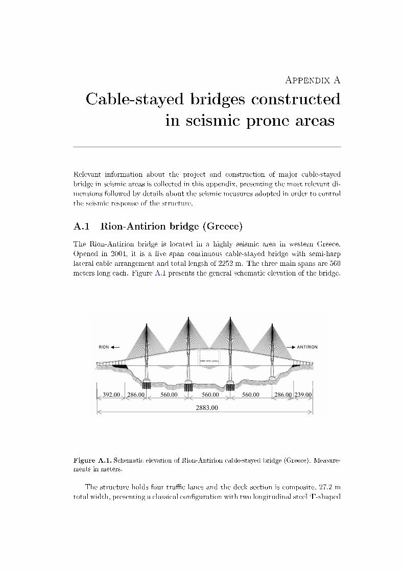
The Rion-Antirion bridge is located in a highly seismic area in western Greece.Opened in 2004, it is a ve span continuous cable-stayed bridge with semi-harplateral cable arrangement and total length of 2252 m. The three main spans are 560meters long each. Figure A.1 presents the general schematic elevation of the bridge.
Figure A.1. Schematic elevation of Rion-Antirion cable-stayed bridge (Greece). Measure-
ments in meters.
The structure holds four trac lanes and the deck section is composite, 27.2 mtotal width, presenting a classical conguration with two longitudinal steel `I'-shaped

310 Appendix A. Constructed cable-stayed bridges
2.2 m high edge girders separated 22.1 m where cable anchors are directly attached.Transverse metallic beams of the deck are disposed between both longitudinal girderseach 4.06 m. Upper concrete slab is 25 cm thick.
Very high longitudinal stiness has been conferred to the towers in order to solvethe characteristic problem of the reduced stiness along this direction in a multiple-span cable-supported bridge. Such stiening is obtained by means of four concretelegs joined with a special composite element on the top of the tower, which enclosesthe anchors of the cable-system and increases the stability when the structure issubjected to static or dynamic actions.
Anti-seismic measures in Rion-Antirion bridge
Seismic action governed the project of this structure. The bridge was designed toresist an earthquake with moment magnitude equal to 7, 0.48 g in terms of PGA,and transverse tectonics movements between consecutive towers of 2 meters. Theresponse spectrum employed in the design has an extreme spectral acceleration of1.2 g and a return period of 2000 years. Both local subsoil eects and soil-structureinteraction were taken into account.
The deck is completely suspended by the cable-system in vertical direction, whichtogether with the great stiness projected in the towers, makes it safe to rely on suchmonolithic elements in longitudinal direction, whilst Viscous uid Dampers (VD)control transverse movements (Virlogeux, [Virlogeux 2001]). Hence a partial isola-tion has been selected, combining dissipation devices with allowed seismic demandin the towers (section 2.3.).
Due to the great importance of the bridge, many research works have been con-ducted about its seismic response; [Infanti 2004] [Morgenthal 1999] [Combault 2005][Dobry 2003] [Lecinq 2003] [Pecker 2004], among others.
The seismic control system is equipped with passive devices; viscous dampers(VD) plus fuse restrainers in parallel which establish the transverse connection be-tween the deck and each tower. Fuse restrainers have been designed to behave likesti links dealing with moderate earthquakes or strong winds, limiting this way theserviceability displacements (SLS). However, if the structure is subjected to the de-sign earthquake action (with an associated return period larger than 350 years) fuserestrainers fail, releasing the free movement of the dampers to maximize the energydissipation, being necessary their substitution after the ground motion.
The deck is not vertically linked to the towers as it was already mentioned;instead it is completely supported by the stays in order to maximize the eective-ness of the cable-system and the global seismic response (see section 2.2.6). Intransverse direction, dissipation devices are disposed in deck-tower connection inorder to restrict the relative movements of the deck under severe earthquakes; inlongitudinal direction, the deck is free in its whole length (2252 meters) trying toaccommodate tectonic and thermal movements, designing the neoprene expansionjoints over the abutments to admit movements up to 5 meters under strong earth-quakes [Combault 2005].

A.1. Rion-Antirion bridge 311
Each transverse deck-tower connection has 4 viscous dampers (VD) and one fuserestrainer. VD located in the towers have an extreme reaction capacity of 3500 kN,±1750 mm maximum stroke and damping constant Cd = 3000 kN/(m/s)0.15 each,whilst fuse restrainers fail when their force reach 10500 kN.
Each connection of the deck and the transition piers in the approach viaductisolate the deck with elastomeric bearings which increase the vibration periods andreduce the spectral accelerations, moreover, VD are incorporated in order to dissi-pate energy and a fuse restrainer is integrated inside one of the dampers. These arethe technical data of the seismic devices in the transition piers: two VD (Fmax=3500kN, ±2600 mm stroke), one fuse restrainer (Fmax=3400 kN) and elastomeric bear-ings.
The controlling parameter of VD nonlinear response αd, repeated below theconstitutive expression for convenience, is low (αd = 0.15) in order to obtain a greatdissipation of energy and a nearly constant force for a wide range of velocities. Thework of Infanti et al [Infanti 2004] collects detailed information about the mechanicalcharacteristics of VD and fuse restrainers employed in Rion-Antirion bridge, alongwith the results of the laboratory test conducted in such elements (fatigue tests).
Fd = Cd |x|αd sign (x) (A.1)
Where Fd is the reaction of the damper, Cd is the damping constant and x therelative velocity.
Fuse restrainers have spherical hinges in their ends in order to ensure the align-ment of the load and the fuse axis (bending is not allowed in this element). Thesedevices are designed to resist the same stroke than the dampers, trying to avoidtheir destruction during extreme ground motions. They admit a readjustment of itslength to allow slow tectonic movements without introducing forces in the deck.
Figure A.2, taken from the report of Infanti et al [Infanti 2004], illustrates theseismic devices installed in deck-tower and deck-transition pier connections.
Other seismic devices in Rion-Antirion bridge are the dampers inside the an-chorages of the cables, which increase their small damping to limit their vibrations[Lecinq 2003].
It was observed that, if the extreme design earthquake occurs during the con-struction of the towers, before joining the four legs, three of them could be subjectedto tensile stresses and the fourth might resist all the compressive load. In light ofthese numerical results, it was decided to reinforce and prestress such legs strongly;furthermore, a powerful bracing system between these elements was set during theconstruction [Combault 2005].
The foundation has been established over exceptionally soft and deep soil, whichhas been improved by introducing metallic columns with 20 to 30 m high. Suchcolumns are not connected to the concrete foundation of the towers (with a diameterof 90 m), they are separated by a layer of gravel (2.8 m thick) forming a sort of plastichinge if the extreme design earthquake strikes [Dobry 2003] [Pecker 2004].

312 Appendix A. Constructed cable-stayed bridges
Figure A.2. Seismic control system in the connection of the deck with the towers (left)
and transition piers (right). Taken from the report of Infanti et al [Infanti 2004].
A.2 Memorial Bill Emerson bridge (USA)
Memorial Bill Emerson bridge (opened to trac in 2003) crosses over Mississippiriver and has two lateral cable planes with semi-harp arrangement and `H'-shapedtowers. The main span is 351 meters, both lateral spans are 143 m long and thelength of the approach viaduct is 570 m. The deck is composite, 29.3 m wide andholds road trac. Figure A.3 shows the schematic bridge elevation and the cross-section of its deck.
Anti-seismic measures in Memorial Bill Emerson Bridge
This bridge is close to an active fault and important seismic risk is present in thearea, the structure has been designed to resist earthquakes of moment magnitudehigher than 7.5. The bridge is equipped with 84 accelerometers which monitor itsreal-time response under any kind of action, being an important data source in thestudy of the seismic behaviour of cable-stayed bridges [Chen 2007] [Çelebi M. 2005].A good agreement between the reality of the structure and nite element predictionswas achieved in light of the response obtained when it was subjected to a signicantground motion in 2005 [Chen 2007].
Each deck-tower connection employs 8 Shock Transmission Units (STU) in lon-gitudinal direction (parallel to the trac), with a capacity of 6670 kN and ±180 mmstroke each, disposing a sti link transversely. The deck is joined to the towers invertical direction by means of two POT supports. The connection between the deck

A.2. Memorial Bill Emerson bridge 313
Figure A.3. Elevation scheme of Memorial Bill Emerson (Cape Girardeau) bridge and
typical cross-section of its deck. Measurements in meters.
and the abutments has two retention devices, a xed transverse link and an expan-sion joint in longitudinal direction, allowing the movement along the latter axis andthe rotation about transverse and vertical axes. Therefore, under service loads theconnections release the deck of this bridge in longitudinal direction and x it trans-versely, whilst under important earthquake the deck is also restrained longitudinallyby the towers. Figure A.4 summarizes the seismic strategies employed in the bridge.
A benchmark problem about the incorporation of passive, active, semi-active de-vices, or a combination of them (hybrid control) in this bridge was proposed. Manyresearchers have published works with dierent possibilities, here just some refer-ences are collected: [Caicedo 2003] [Dyke 2003] [Jung 2003] [Park 2003a] [Park 2003b][Agrawal 2002] [He 2001], among others. The interested reader is referred to thewebsite http://mase.wustl.edu/wusceel/quake/bridgebenchmark/index.htm formore information, including the description of the benchmark problem stages, dy-namic models implemented in Matlab [Matlab 2011] and several papers with dier-ent proposals. The rst stage of the problem exclusively considers the longitudinalcomponent of the earthquake, which is the most demanding one in this case, whilstin the second stage the three-directional seismic excitation and its spatial variabilitywere considered (it was also included the dynamic eect of snow live load over thedeck increasing the mass and hence the vibration period).

314 Appendix A. Constructed cable-stayed bridges
aab b b. Shock Transmission Units (STU)
in longitudinal direction
a. Stiff link in transverse direction
Stiff link (transv.)Expansion joint (longitudinal)
Stiff link (transv.)
Expansion joint (longitudinal)
Stiff link (transv.)
STU (longitudinal)
Figure A.4. Seismic devices equipped in Memorial Bill Emerson bridge.
A.3 Tsurumi Fairway bridge (Japan)
The length of Tsurumi Fairway bridge is 1020 m being the main central span 510 m.One central cable plane in semi-harp arrangement has been disposed. It was openedto trac in 1994. Figure A.5 represents the schematic elevation of the structure.
Figure A.5. Schematic elevation of Tsurumi Fairway bridge (Japan). Measurements in
meters.
The deck section is a metallic box with enough torsional stiness to resist theeccentric forces which the central cable-system is unable to withstand. The totalwidth of the deck is 38 m and the height 4 m. It is designed to support road trac.
The pylons are inverted `Y'-shaped towers with lower diamond, they are made

A.4. Yokohama Bay bridge 315
of steel above the vertical pier, which is composite. The foundation is made ofreinforced concrete.
Anti-seismic measures in Tsurumi Fairway bridge
The structure is located in an area with important seismicity; it is designed to resistearthquakes up to 8.2 moment magnitude with a return period of only 75 years.
In the future, the construction of a twin bridge close to this one is foreseen,which makes the transverse space available for deck-tower connections very reduced(see gure A.6), being necessary the limitation of relative movements. With thisobjective in mind, horizontal cables are disposed linking the deck and the towerin longitudinal direction, parallel to the axis of the former and inside its section.Four cables are anchored to each tower, two along one side of the deck and theother two along the opposite, as it may be observed in gure A.6, where deck-towerconnection and vertical pier are detailed. The length of each cable is 117 m andtheir total diameter 167 mm. Their initial prestress was projected in order to keepthe tension below the failure level during extreme earthquakes [Enomoto 1994].
Two vane-type dampers (VD) are installed over the metallic part of the towerbelow the deck as it is observed in gure A.6, whilst gure A.7 depicts details oftheir shape and constitutive behaviour. Such dampers help to reduce the longitu-dinal oscillation of the deck, transforming this movement in a rotation about thetransverse axis in the devices. The longitudinal reaction introduced in the deck bythe dampers is proportional to the square of the relative velocity (αd = 2) up to alimit value of the force (Fmax = 2000 kN), beyond this level the reaction is main-tained constant as long as the velocity increases, releasing pressure through orices.The parabolic response of the damper causes low reactions under slow movements(wind or moderate earthquakes) and a strong increase under important seismic in-tensities (see gure A.7), acting as shock transmission units (STU). Seismic analysisconcluded that horizontal displacements are reduced by 30 % if these dampers areincorporated [Enomoto 1994]. The damping constant of the vane-type damper isCd = 104 kN/(m/s)2.
The deck is xed to the towers in vertical and transverse directions.
A.4 Yokohama Bay bridge (Japan)
Yokohama Bay bridge (nished in 1989) is a cable-stayed structure with three spans,the central one is 460 m and laterals are 200 m long. In gure A.8 the elevation ofthis structure is schematically represented.
The deck is a metallic sti truss which supports 6 road trac lanes in the upperpart and two in the lower level. The `H'-shaped towers are metallic and the cable-system is lateral with semi-harp arrangement.

316 Appendix A. Constructed cable-stayed bridges
Figure A.6. Detail of deck-tower connection and vertical pier in Tsurumi Fairway bridge
(taken from the work of Enomoto et al [Enomoto 1994]).
Dam
per
for
ce;F
Relative velocity;v
unit
Control pressure
Figure A.7. Left: Detail of vane-type dampers (VD) employed in Tsurumi Fairway bridge
(taken from the work of Enomoto et al [Enomoto 1994]). Right: Constitutive properties of
equipped vane dampers.

A.4. Yokohama Bay bridge 317
Figure A.8. Elevation scheme of Yokohama Bay bridge. Measurements in meters.
Anti-seismic measures in Yokohama Bay bridge
This structure belongs to a key infrastructure network between Tokyo and Yoko-hama, and it is located in a highly seismic area. It was designed and constructedbefore Great Hanshin (Kobe) earthquake in 1995, and therefore the eect of near-eld records was not considered (this eect was introduced in the Japanese seismiccode before such event), the design earthquake intensity was neither as strong as theone recorded in Kobe signals. A detailed seismic analysis considering the reducedstiness of the soil and the important height of the gravity center of the structurewas performed.
The link between the deck and the towers, and also between this element andthe transition piers at the end of cable-stayed length, is executed by means of Link-Bearing Connections (LBC). The purpose of these devices is to release longitudinallythe deck during strong ground motions in order to reduce the inertia forces whichmay be introduced in the towers and the abutments by the deck, increasing thelongitudinal vibration modes (hence reducing associated spectral acceleration) andmagnifying displacements. The length of LBC is limited to 2 meters in order toprevent excessive seismic movements. This connection releases the deck under slowactions like thermal eects. Figure A.9 includes the dimensions in millimeters ofLBC equipped in the towers, the points were they are located along the deck andone picture with their disposition in the tower.
The behaviour of LBC is nonlinear due to the change of direction of the strongaxial load generated when the deck is moved (geometric nonlinearity). In gure A.10,taken from the work of Yamaguchi and Furukawa [Yamaguchi 2004], the nonlinearreal behaviour of LBC and its linearized response, which was employed in the designstage, may be observed.
The vertical movement of the deck is free in the connections, suspended fromthe cable-system. Transversely, the deck is xed to the towers.
The research of Fujino and Siringoringo [Fujino 2006], based on recorded re-sponse data of Yokohama Bay bridge under 14 earthquakes with dierent intensity

318 Appendix A. Constructed cable-stayed bridges
Figure A.9. Dimensions (in mm) of LBC disposed in the towers of Yokohama Bay bridge
(left). Points along the bridge where LBC are equipped (top right corner). Picture including
the LBC joining the deck and the tower (bottom right corner).
Figure A.10. Left: Geometric eects associated with LBC response in Yokohama Bay.
Right: Nonlinear and linear (design) response of LBC. Taken from the work of Yamaguchi
and Furukawa [Yamaguchi 2004].

A.5. Ting Kau bridge 319
levels, demonstrated that LBC releases the deck if the structure is subjected tostrong records, however under moderate events the connections constrain the deckin one or both two transition piers, increasing considerably the bending momentproduced in them, which is able to exceed even the value recorded under strongearthquakes. This failure is probably due to the friction, which leads to the follow-ing observed behaviour; under strong records LBC initially releases the deck as itwas expected, but several seconds before it is xed when the intensity is reduced.
Otsuka et al [Otsuka 2004] conducted a seismic analysis about this bridge withacceleration spectra adapted to the modern seismic Japanese code, proposing thestrengthening of transition piers and upper transverse struts in the towers, amongother considerations.
Yamaguchi and Furukawa [Yamaguchi 2004] studied the seismic behaviour ofYokohama Bay structure by means of two-dimensional analysis, verifying the in-adequate response when the acceleration design spectra compliant with modernJapanese seismic code is employed, presenting excessive longitudinal movements ofthe deck, the yielding of both towers at foundation level and transition piers besidesthe loss of tension in several cables. The installation of viscous dampers (VD) inall LBC was proposed, observing numerically the remarkable improvement of theseismic behaviour if care is taken in the design of VD properties in order to avoidexcessive stresses in transition piers.
The fundamental period of this bridge is longitudinal, approximately 8 s, due tothe free movement of the deck with respect to the supports in this direction. Thislong period governs its dynamic response.
A.5 Ting Kau bridge (China)
Ting Kau bridge is a multiple-span cable-stayed structure with 4 spans located inHong-Kong and opened to trac in 1998. Main central spans are 448 and 475 mlong respectively, whilst lateral spans are 127 m each, composing a total length of1177 m.
Its distinctive characteristic is the employment of diagonal stabilization cablesto increase the longitudinal stiness of the bridge, constraining the movement ofthe upper level of the central tower (see section 2.2.8). Altogether, 8 longitudinalstabilization cables are disposed linking the top section of the central tower and thearea close to the connection of the deck with both lateral towers. The length of suchdiagonal cables, 465 m, established a record [Yuen 2007].
The towers are single concrete masts which separate both sides of deck section(gure A.11). The selection of this kind of towers meets the requirement of a struc-ture with reduced surface due to wind considerations. Transverse cable-system wasintroduced in order to stabilize the slender masts in transverse direction, joining theupper section with the sti lower area of the tower below the deck (gure A.11).
The deck is a composite twin-box section; the boxes are separated 5.2 metersand connected through transverse metallic struts. Each side of the deck is 18.77 m
320 Appendix A. Constructed cable-stayed bridges
wide and holds three trac lanes plus one emergency lane. Longitudinal metallicgirders of the deck are 1.75 m deep. Four lateral cable planes are disposed, anchoringtwo at both sides of the deck section. The semi-harp cable-arrangement presents aseparation between cables of 13.5 m.
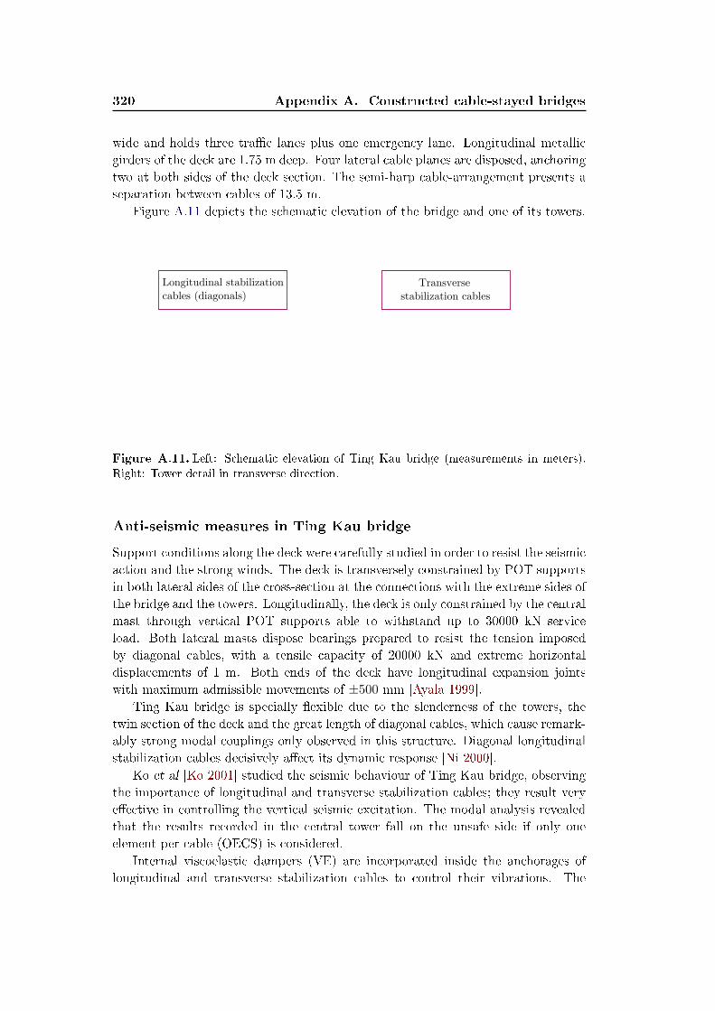
Figure A.11 depicts the schematic elevation of the bridge and one of its towers.
Longitudinal stabilizationcables (diagonals)
Transverse stabilization cables
Figure A.11. Left: Schematic elevation of Ting Kau bridge (measurements in meters).
Right: Tower detail in transverse direction.
Anti-seismic measures in Ting Kau bridge
Support conditions along the deck were carefully studied in order to resist the seismicaction and the strong winds. The deck is transversely constrained by POT supportsin both lateral sides of the cross-section at the connections with the extreme sides ofthe bridge and the towers. Longitudinally, the deck is only constrained by the centralmast through vertical POT supports able to withstand up to 30000 kN serviceload. Both lateral masts dispose bearings prepared to resist the tension imposedby diagonal cables, with a tensile capacity of 20000 kN and extreme horizontaldisplacements of 1 m. Both ends of the deck have longitudinal expansion jointswith maximum admissible movements of ±500 mm [Ayala 1999].
Ting Kau bridge is specially exible due to the slenderness of the towers, thetwin section of the deck and the great length of diagonal cables, which cause remark-ably strong modal couplings only observed in this structure. Diagonal longitudinalstabilization cables decisively aect its dynamic response [Ni 2000].
Ko et al [Ko 2001] studied the seismic behaviour of Ting Kau bridge, observingthe importance of longitudinal and transverse stabilization cables; they result veryeective in controlling the vertical seismic excitation. The modal analysis revealedthat the results recorded in the central tower fall on the unsafe side if only oneelement per cable (OECS) is considered.
Internal viscoelastic dampers (VE) are incorporated inside the anchorages oflongitudinal and transverse stabilization cables to control their vibrations. The

A.6. Stonecutters bridge 321
bridge is equipped with more than 200 sensors which give information of its responseunder wind, earthquake, live loads, etc.
A.6 Stonecutters bridge (China)
Stonecutters bridge, located in Hong Kong and opened in 2009, is nowadays thesecond longest cable-stayed bridge in the world with a main span of 1018 m. Lat-eral spans present intermediate piers to retain the central one and are both 289 mlong. Two lateral cable planes with semi-harp arrangement has been disposed. Thedistance between consecutive cables in central and lateral spans is 18 m and 10 mrespectively.
The towers are single masts with circular concrete section in the lower andintermediate levels, and composite with stainless steel cover in the upper area whereanchorages are located. The incorporation of concrete in this part of the towerincrease the damping in comparison with the solution exclusively metallic.
Auxiliary piers in lateral spans are approximately 60 m high and their exibilityis enough to prevent the use of sliding bearings in their connection with the deck,which is completely encastred. Transition piers (in both extremes of the cable-stayed length) are gantry structures to provide lateral stability and enough surfaceto install the support devices of approach viaducts.
The deck section is a twin box; metallic in the central span and made of concretein the lateral spans to counteract the weight of the main one. Altogether 6 traclanes (3 per both sides of the twin section) are supported. In the main span thetotal width of the deck is 51 meters and the height of the section reaches 3.9 m inthe transverse struts linking both sides of the girder.
Figure A.12 presents the elevation scheme of Stonecutters bridge
Figure A.12. Elevation scheme of Stonecutters bridge. Measurements in meters.
Anti-seismic consideration in Stonecutters bridge
Stonecutters bridge is located in a seismic prone area. The completely elastic re-sponse of the structure under moderate earthquakes was required in the design, with

322 Appendix A. Constructed cable-stayed bridges
120 years return period (Serviceability Limit State), and admitting some yielding incertain parts of the towers but requiring its repair without interrupting the serviceunder strong seismic events, with 2400 years return period (Ultimate Limit State).If the structure is subjected to an extreme earthquake, with 6000 years return pe-riod, the structural integrity is required in order to support the access of healthpersonnel (Extreme Limit State) [Hansen 2007]. Therefore, partial isolation (miti-gation through seismic devices and structural dissipation) is applied to the seismicdesign.
The eects of spatial variability of the seismic action were taken into accountdue to the great length of the bridge.
The deck-tower connection is solved by means of sliding bearings (SB) in trans-verse direction, and longitudinally through 4 Shock Transmission Units (STU) withvelocity exponent αd = 2 [Colato 2008]. These STU act only under fast dynamicsolicitations (earthquake or wind) and release the deck under slow movements (ther-mal eects, creep, shrinkage, etc.). The relative movement between the deck andthe towers is free in vertical direction [Hussain 2002]. Figure A.13 presents theconguration of such connection.
Figure A.13. Detail of deck-tower connection in Stonecutters bridge.
Internal dampers have been installed in the anchorage of the cables in orderto increase their damping, obtaining a critical damping factor of 4 %. The risk ofresonance in some cables due to wind or even earthquake excitations was observed,since their fundamental local frequency was close to the excitation of the anchorages(or half this value), this problem was prevented using Tuned Mass Dampers (TMD)to increase the excitation period in the towers.

Appendix B
On the dimensions and
characteristics of the proposed
bridges
A large number of cable-stayed bridges have been studied in this thesis, among theircharacteristics dimensions there are variable parameters (like the tower shape), andalso canonical proportions which are taken from constructed cable-stayed bridgesand maintained constant since they are not the object of the study.
The most signicant parameters of the proposed cable-stayed bridges are de-scribed in this appendix, including the bridge geometry, the spring stiness repre-senting the tower foundations, and the calculation of the cable properties, amongother valuable information.
B.1 Tower height and span distribution
Both towers have the same dimensions in all the models, which are in turn completelysymmetric about the vertical plane crossing the span center transversely (Y ) andalso about the vertical plane along the longitudinal axis of the deck (X).
The classical canonical relationship between the height of the towers above thelevel of the deck (H) and the main span (LP ), as well as the ratio between the mainand the lateral spans (LS) was suggested by Como et al [Como 1985] more than twodecades ago:
H
LP=
1
5;LSLP
=1
3(B.1)
Nowadays, the trend is to increase the size of the towers as it is observed intables B.1 and B.2 [Manterola 1994], where the mentioned ratios are obtained inseveral constructed cable-stayed bridges worldwide. In light of these two tables,it has been decided to modify the classical parameters proposed by Como et al,considering instead the followings:
H
LP=
1
4.8;LSLP
=1
2.5(B.2)
The height of the towers between the deck level and the foundation (Hi) isdetermined by the local conditions and the trac which is expected to cross belowthe bridge, among other factors. It is very important in dynamic calculations, since

324 Appendix B. Dimensions and characteristics of the models
Ratios
Bridge LP LS
Deck Deck Tower H
LP
h
LP
LS
LPheight; h width; B height; H
Jacksonville∗ 396 198 1.52 32.0 90.0 1/4.33 1/264 1/2.00
Diepoldsau 97 40.5 0.55 14.5 28.7 1/3.38 1/176 1/2.39
Skarnsundet 530 190 2.15 11.3 105.0 1/5.00 1/246 1/2.79
Helgeland 425 177.5 1.36 12.0 89.3 1/4.75 1/310 1/2.39
Guadiana 324 135 2.50 18.0 77.0 1/4.20 1/129 1/2.40
Sama Langreo∗ 130∗ 65 1.20 14.2 48.0 1/5.40 1/216 1/4.00
Arade 256 107 1.63 17.0 52.6 1/4.80 1/157 1/2.39
Yobukoh 250 121 2.20 10.9 62.6 1/4.00 1/113 1/2.10
C. Saone 151.8 44.8 1.03 15.5 33.3 1/4.55 1/146 1/3.39
G. Isere∗ 103∗ 67 1.90 11.8 38.0 1/5.40 1/108 1/3.07
Centenario 265 102 2.70 22.0 60.0 1/4.40 1/98 1/2.60
Table B.1. Summary of the dimensions and geometric ratios in Lateral Cable Plane (LCP)
cable-stayed bridges. Measurements in meters. The symbol (∗) denotes that the bridge has
only one tower and hence the main span has been doubled in the calculation of the ratios.
The symbol (h) indicates harp-cable assembly (the rest are semi-harp). Adapted from the
work of Manterola [Manterola 1994].
Ratios
Bridge LP LS
Deck Deck Tower H
LP
h
LP
LS
LPheight; h width; B height; H
Tampa 363 164 4.47 28.8 73.7 1/4.92 1/181 1/2.21
Aomori 240 128 2.5-3.5 25.0 64.3 1/3.73 1/68-1/96 1/1.87
Coatzacoalcos 288 112 3.30 18.0 61.3 1/4.68 1/87 1/2.57
Usui∗ 111 111 2.50 21.4 61.0 1/3.63 1/88 1/2.00
Wandre∗ 168 144 3.30 21.8 79.0 1/4.25 1/100 1/1.93
Elorn 400 100 3.47 23.1 83.0 1/4.81 1/115 1/4.00
Chandoline 140 72 2.50 27.0 30.4 1/4.61 1/56 1/1.95
Elba 123 61 2.50 32.3 28.0 1/4.40 1/49 1/2.01
Table B.2. Summary of the dimensions and geometric ratios in Central Cable Plane (CCP)
cable-stayed bridges. Measurements in meters. The symbol (∗) denotes that the bridge has
only one tower and hence the main span has been doubled in the calculation of the ratios.
All the bridges have semi-harp cable congurations. Adapted from the work of Manterola
[Manterola 1994].
B.2. Cross-section of the deck 325
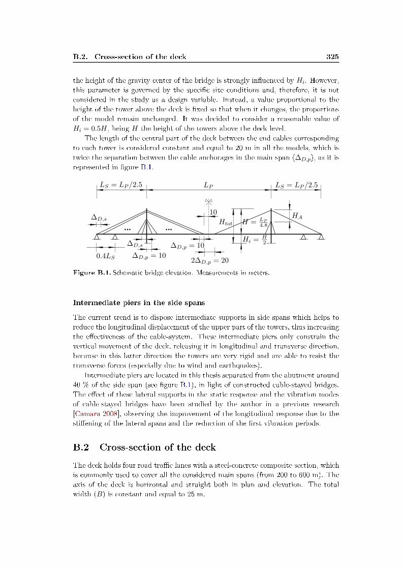
the height of the gravity center of the bridge is strongly inuenced by Hi. However,this parameter is governed by the specic site conditions and, therefore, it is notconsidered in the study as a design variable. Instead, a value proportional to theheight of the tower above the deck is xed so that when it changes, the proportionsof the model remain unchanged. It was decided to consider a reasonable value ofHi = 0.5H, being H the height of the towers above the deck level.
The length of the central part of the deck between the end cables correspondingto each tower is considered constant and equal to 20 m in all the models, which istwice the separation between the cable anchorages in the main span (∆D,p), as it isrepresented in gure B.1.
Figure B.1. Schematic bridge elevation. Measurements in meters.
Intermediate piers in the side spans
The current trend is to dispose intermediate supports in side spans which helps toreduce the longitudinal displacement of the upper part of the towers, thus increasingthe eectiveness of the cable-system. These intermediate piers only constrain thevertical movement of the deck, releasing it in longitudinal and transverse direction,because in this latter direction the towers are very rigid and are able to resist thetransverse forces (especially due to wind and earthquakes).
Intermediate piers are located in this thesis separated from the abutment around40 % of the side span (see gure B.1), in light of constructed cable-stayed bridges.The eect of these lateral supports in the static response and the vibration modesof cable-stayed bridges have been studied by the author in a previous research[Camara 2008], observing the improvement of the longitudinal response due to thestiening of the lateral spans and the reduction of the rst vibration periods.
B.2 Cross-section of the deck
The deck holds four road trac lanes with a steel-concrete composite section, whichis commonly used to cover all the considered main spans (from 200 to 600 m). Theaxis of the deck is horizontal and straight both in plan and elevation. The totalwidth (B) is constant and equal to 25 m.

326 Appendix B. Dimensions and characteristics of the models
The design of the deck section in bridges with lateral cable planes (LCP) is inaccordance with the current trend in constructed cable-stayed bridges, disposingtwo longitudinal edge steel girders and one upper concrete slab. On the other hand,the cross-section of the deck adopted in structures with central cable plane (CCP)is an `U'-shaped steel section below the concrete slab, which is able to withstandthe torsion that is not resisted by the cable-system.
Tables B.1 and B.2 included the ratio between the height of the deck (h) andthe main span (LP ) in constructed cable-stayed LCP and CCP bridges. As itmay be observed, the height of the deck is higher in structures with central cablearrangement (CCP) since the torsional resistance is entrusted to the deck. Theaveraged deck ratios from these tables are:
h
LP=
1
180→ LCP (B.3)
h
LP=
1
90→ CCP (B.4)
However, expression (B.3) is questionable since, in real projects, the depth of thedeck in LCP cable-stayed bridges is nearly independent of their main span, instead itis inuenced by the transverse and longitudinal distance between consecutive cableanchorages. Nonetheless, the depth of the deck slightly increases with the main spanbecause of the increment in the length of the cables and the consequent increase ofthe exibility, which requires a stier deck due to wind considerations. The workof Astiz [Astiz 2001] suggests the variation of the depth of the deck with the mainspan in several composite LCP cable-stayed bridges:
h = 0.78 + 0.00302LP → LCP (B.5)
Where h and LP are expressed in meters.Static analysis conducted here have veried that the level of stresses in LCP
and CCP composite decks are admissible considering the worst situation; imposingthe self-weight and the live load in the central part of the bridge, where the dis-tance between cable anchorages is larger (20 meters). Therefore, the relationshipbetween the depth of the deck and the main span in LCP models proposed by Astiz(expression (B.5)) and the ratio presented in equation (B.4) for CCP models areaccepted.
Figure B.2 presents the considered sections of the deck in both LCP and CCPmodels (excluding the non-structural mass), being their principal dimensions con-stant or variable in terms of the main span. The dimensions of the longitudinal andtransverse girders in LCP deck cross-sections, or the plate thickness and stienersin CCP models, are the result of the simplied elastic static analysis mentionedabove (with 20 m span), preventing the extreme stresses from exceeding the designallowable values. The longitudinal separation of the cables at the level of the deckwas expressed in gure B.1 and discussed further in section B.5.

B.3. Dimensions of the towers 327
Cables every 10 m in the main spanand every in lateral spans
0,2
Diaprhagms each 5 m in themain span, and eachin the lateral spans
2
Profiles of the diaphragm:
Vertical: 2 UPN 200Diagonal: 2 UPN 300
everyevery
every
*
*
*
every
(a) Deck cross-section for LCP arrangement
Cables every 10 m in the main spanand every in lateral spans
0,2
Diaprhagms each 5 m in themain span, and eachin the lateral spans
2
Profiles of the diaphragm:
Vertical: 2 UPN 200Diagonal: 2 UPN 300
*
*
*
every
(b) Deck cross-section for CCP arrangement
Figure B.2. Composite deck cross-sections employed in lateral and central cable congu-
rations, parameterized in terms of the main span (LP ). Measurements in meters.(*) Plate
thickness is larger at localized areas; this is a mean value for analysis.
B.3 Dimensions of the towers
The dimensions of the towers in proposed models are obtained from the specicstudy of a set of constructed cable-stayed bridges, which is deemed representativeof each studied tower shape and cable-system arrangement. The geometric ratios,which lead to the nal cross-sections and proportions of the towers, are presented

328 Appendix B. Dimensions and characteristics of the models
here in tables B.3 to B.8 and graphically in gures B.3 to B.7.The cable-system assembly is always semi-harp, trying to minimize the length
of the area where the anchorages are located (HA) in order to maximize the eec-tiveness of the cables. Therefore, the distance between anchorages in the tower isreduced to a minimum space which allows the construction. In these bridges, suchdistance is reasonably ∆T = 2 m, which xes the length of the anchorage area inthe tower:
HA = ∆T (NT − 1) (B.6)
Where NT is the number of stays per half main span and cable-plane (obtainedwith the expression NT = (LP −20)/20, justied in section B.5) which depends1 onthe main span LP .
If the area of the tower where the anchorages are located is not vertical butforms an angle α < 90 with the horizontal line2 (being this value included in thegeometrical description of each tower in gures B.3 to B.7), the length HA is:
HA = ∆T (NT − 1) sin(α)︸ ︷︷ ︸≈1
(B.7)
Due to the large number of cable-stayed bridges studied in this thesis, and therequired parametrization, the design simplicity is strongly recommended. Hence,constant sections between dierent parts of the towers have been considered in theparametric denition. To facilitate the comparison of the results between modelswith dierent towers, the sections have been established as similar as possible.
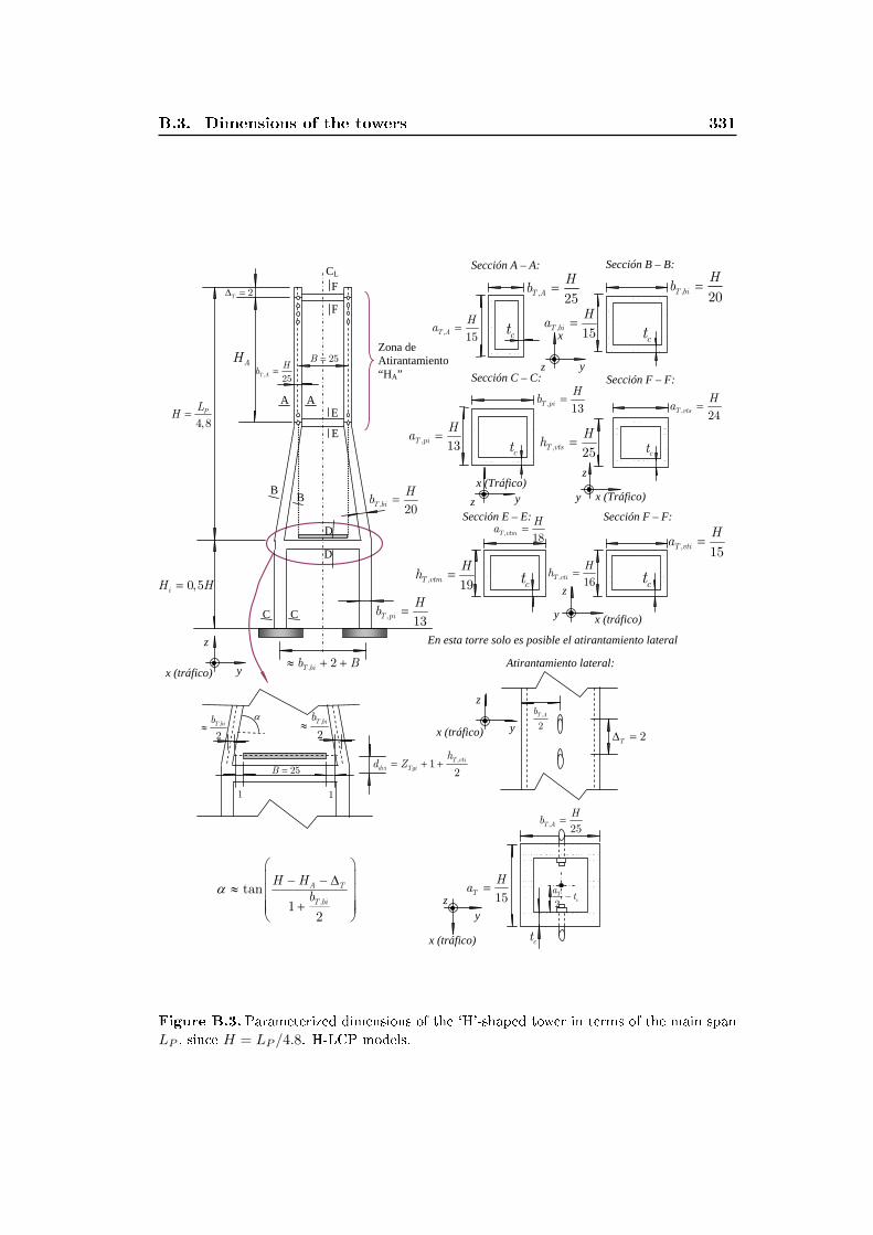
The proportions and sections of `H'-shaped towers in terms of the height abovethe deck, which in turn depends on the main span (H = LP /4.8), have been obtainedfrom a set of bridges with the same type of towers, included in tables B.3 and B.4,along with the ratios proposed here (X, Y and Z are the longitudinal, transverse andvertical directions respectively). The nal version of the `H'-shaped tower employedin the thesis is illustrated in gure B.3.
The proportions of the `Y-shaped' towers with and without lower diamond ofseveral cable-stayed bridges are summarized in tables B.5 and B.63, including theproposed ratios used in the nal version of the towers employed in the thesis, whichare presented in gures B.4 and B.5.
Finally, the dimensions of the `A'-shaped towers with and without lower diamondin several cable-stayed bridges are presented in tables B.7 and B.8, besides theproposed parameters employed in this work which are illustrated graphically ingures B.6 and B.7.
1The number of cables is also inuenced by the vertical connection between the deck and thetower; if it is xed in vertical direction, the closest pair of stays at each side of the tower areeliminated, compared with the solution with free vertical connection (the one employed here).
2The angle between the legs above the deck and the horizontal line, α, has been referred as βbin chapter 7. For convenience, the notation α is maintained in this appendix.
3Again, (∗) denotes that the bridge has only one tower and hence the main span has beendoubled in the calculation of the ratios.

B.3. Dimensions of the towers 329
Bridge LP H
Anchorage Inclined Lower
area legs piers
a (X) b (Y ) a (X) b (Y ) a (X) b (Y )
Barrios de Luna, 1983 440 90 H/24 H/20 H/20 H/18 H/15 H/16
Suez Canal, 2001 404 80 H/18 H/32 H/13 H/16 H/11 H/11
Bill Emerson, 2003 351 75 H/11 H/27 H/11 H/23 H/11 H/10
Yokohama Bay, 1989 460 105 H/20 H/26 H/17 H/26 H/15 H/18
Sidney Lanier, 2003 375 87 H/13 H/31 H/13 H/23 H/13 H/13
Proposed H/15 H/25 H/15 H/20 H/13 H/13
Table B.3. Dimensionless proportions of several cable-stayed bridges with `H'-shaped tow-
ers and proposed ratios in this study. `Inclined legs' refers to the part of the tower between
the anchorage area and the lower strut, `lower piers' refers to the legs of the tower below
the lower strut. Parameters detailed in gure B.3. Measurements in meters.
Bridge LP H
Upper Intermediate Lower
strut strut strut
a (X) h (Z) a (X) h (Z) a (X) h (Z)
Barrios de Luna, 1983 440 90 H/24 H/25 H/22 H/22 - -
Suez Canal, 2001 404 80 - - H/19 H/19 H/17 H/17
Bill Emerson, 2003 351 75 - - H/14 H/17 H/15 H/15
Yokohama Bay, 1989 460 105 - - H/26 H/21 H/21 H/17
Sidney Lanier, 2003 375 87 - - H/15 H/19 H/15 H/16
Proposed H/24 H/25 H/18 H/19 H/15 H/16
Table B.4. Dimensionless proportions of cable-stayed bridges with `H'-shaped towers and
proposed ratios (continued). Parameters detailed in gure B.3. Measurements in meters.
Bridge LP H
Anchorage Inclined Lower
area legs piers
a (X) b (Y ) a (X) b (Y ) a (X) b (Y )
Rijeka Dubrovacka, 2002 244∗ 93 H/18.6 H/16.6 H/18.6 H/23.3 H/18.6 H/23.3
Boine, 2003 170∗ 71 H/16.9 H/8.9 H/16.9 H/19.2 H/14.2 H/14.8
Rhein 335∗ 115 H/28.7 H/14.4 H/28.7 H/29.4 - -
Flehe, 1979 368∗ 130 H/20.2 H/16.4 H/20.2 H/24.4 H/20.2 H/24.4
Wandre, 1989 168∗ 79 H/19 H/19.7 H/19 H/24.6 H/19 H/24.6
Incheon, 2009 800 171 H/21 H/28.4 H/21 H/34 H/21 H/21
Proposed H/18 H/13 H/18 H/23 H/18 H/20
Table B.5. Dimensionless proportions of several cable-stayed bridges incorporating `Y'-
shaped towers with and without lower diamond, and proposed ratios in this study. `Inclined
legs'; legs between the anchorage area and the lower strut. `Lower piers'; legs below the
lower strut. Parameters detailed in gures B.4 and B.5. Measurements in meters.

330 Appendix B. Dimensions and characteristics of the models
Bridge LP H
Lower Vertical pier
strut (lower diamond)
a (X) h (Z) a (X) b (Y )
Rijeka Dubrovacka, 2002 244∗ 93 H/18.6 H/31 - -
Boine, 2003 170∗ 71 H/17.7 H/18.2 - -
Rhein 335∗ 115 - - H/28.7 1.4B
Flehe, 1979 368∗ 130 H/20.2 H/23.5 - -
Wandre, 1989 168∗ 79 - - - -
Incheon, 2009 800 171 H/21 H/29 - -
Proposed H/18 H/23 H/15 H/6
Table B.6. Dimensionless proportions of several cable-stayed bridges incorporating `Y'-
shaped towers with and without lower diamond, and proposed ratios in this study (contin-
ued). Parameters detailed in gures B.4 and B.5. Measurements in meters.
Bridge LP H
Inclined Lower
legs piers
a (X) b (Y ) a (X) b (Y )
William Natcher, 2002 366 79.7 H/16 H/29.5 H/12.3 H/17.7
Chao Phraya, 2006 500 120 H/18.4 H/27.3 H/15.5 H/13.6
Jindo, 1984 344 69 H/18 H/34 H/16 H/12.5
Helgeland, 1991 425 90 H/17 H/36 H/15 H/22
Proposed H/18 H/23 H/18 H/20
Table B.7. Dimensionless proportions of several cable-stayed bridges incorporating `A'-
shaped towers with and without lower diamond, and proposed ratios in this study. `Inclined
legs'; legs between the anchorage area and the lower strut. `Lower piers'; legs below the
lower strut. Parameters detailed in gures B.6 and B.7. Measurements in meters.
Bridge LP H
Lower Vertical pier
strut (lower diamond)
a (X) h (Z) a (X) b (Y )
William Natcher, 2002 366 79.7 H/13.3 H/29.5 H/10 H/3.5
Chao Phraya, 2006 500 120 H/20 H/13.3 - -
Jindo, 1984 344 69 H/16 H/12.5 - -
Helgeland, 1991 425 89 H/15 H/25 H/15 H/7.4
Proposed H/18 H/23 H/15 H/6
Table B.8. Dimensionless proportions of several cable-stayed bridges incorporating `A'-
shaped towers with and without lower diamond, and proposed ratios in this study (contin-
ued). Parameters detailed in gures B.6 and B.7. Measurements in meters.
B.3. Dimensions of the towers 331
Zona de Atirantamiento “HA”
CL
, 25T AHb = AH
2TΔ =
4,8PLH =
B B
D
D
C C
, 20T biHb =
, 2T bib B≈ + +
Sección A – A:
y
z
x (tráfico)
y z
xct, 15T AHa =
, 25T AHb =
, 16T vtiHh =
ct
y x (tráfico)
z
25B =
1 1
Atirantamiento lateral:
, 13T piHb =
A A
,
2T bib≈ ,
2T bib≈
α
F
F
Sección E – E:
, 19T vtmHh =
ct
, 18T vtmHa =
En esta torre solo es posible el atirantamiento lateral
E
E
25B =
, 20T biHb =
, 15T biHa =
Sección F – F:
2TΔ =
,
2T Ab
15THa =
, 25T AHb =
ct
2T
ca t−
z
x (tráfico) y
yz
x (tráfico)
y zx (Tráfico)
Sección C – C:
ct
, 13T piHb =
, 13T piHa =
x (Tráfico) y
z
Sección F – F:
ct
, 24T vtsHa =
, 25T vtsHh =
= + + ,12T vti
dvi Tgi
hd Z
Sección B – B:
ct
α
⎛ ⎞⎜ ⎟− − Δ
≈ ⎜ ⎟⎜ ⎟+⎜ ⎟⎝ ⎠
,tan
12
A T
T bi
H Hb
, 15T vtiHa =
0,5iH H=
Figure B.3. Parameterized dimensions of the `H'-shaped tower in terms of the main span
LP , since H = LP /4.8. H-LCP models.

332 Appendix B. Dimensions and characteristics of the models
Zona de Atirantamiento “HA”
CL
AH
TΔ
TΔ
A A
B B
D
D
C C
Sección A – A: Sección B – B:
y
z
x (tráfico)
z y
, 18T AHa =
, 13T AHb =
ct ct
y z
x
ct
Sección C – C:
ct
y x (tráfico)
z
Sección D – D:
= 25B 1 1
Atirantamiento lateral:
Atirantamiento central:
y
z
x , 2 0,8T A cb t− −
,
2T A
c
at−
, 0,42T A
c
bt− −
,
2T bib≈
α
yz
x (tráfico)
x
0,4
,252 2
tani
T piHB bα
≈ + + +
+ + ,12T vti
Tgi
hZ
y
z
x
, 18T biHa =
, 23T biHb =
, 18T piHa =
, 20T piHb =
=, 23T vtiHh
=, 18T vtiHa
, 13T AHb =
, 23T biHb =
, 20T piHb =
ct
ct TΔ TΔ
,
2T bib≈
, 15T AHb = , 15T A
Hb =
, 18T AHa = , 18T A
Ha =
ct ct
,
2T A
c
bt−
α
⎛ ⎞⎜ ⎟− − Δ
≈ ⎜ ⎟⎜ ⎟+ +⎜ ⎟⎝ ⎠
,
2tan1
2 2
A T
T bi
H HbB
,
4T Ab
,
4T Aa
,
2T A
c
at−
4,8PLH =
0,5iH H=
Figure B.4. Parameterized dimensions of the inverted `Y'-shaped tower without lower
diamond in terms of the main span LP , since H = LP /4.8. Y-LCP and Y-CCP models.

B.3. Dimensions of the towers 333
Figure B.5. Parameterized dimensions of the inverted `Y'-shaped tower with lower dia-
mond in terms of the main span LP , since H = LP /4.8. YD-LCP and YD-CCP models.

334 Appendix B. Dimensions and characteristics of the models
Zona de Atirantamiento “HA”
CL
B B
D
D
C C
y
z
x (tráfico) Atirantamiento lateral:
y
z
x (tráfico)
T≈ Δ,
2T bib≈
α
En esta torre solo es posible el atirantamiento lateral
α
2A TH − Δ
y
z
x
Sección A – A:
z y
ct
y z
x
Sección C – C:
y x (tráfico)
z
Sección D – D:
x
yz
x (tráfico)
Sección B – B:
ctA A
Variable
, 18T AHa =
, 18T biHa =
ct, 18T pi
Ha =
, 20T piHb =
4,8PLH =
TΔ
AH
2 TΔ
ct=, 23T vtiHh
=, 18T vtiHa
, 23T biHb =
, 20T piHb =
α
⎛ ⎞⎜ ⎟
≈ ⎜ ⎟⎜ ⎟+ +⎜ ⎟⎝ ⎠
,tan
12 2
T bi
HbB
,252 2
tani
T piHB bα
≈ + + +
= 25B 1 1
,
2T bib≈
+ + ,12T vti
Tgi
hZ
,
2T bib≈
, 15T AHb =
, 18T AHa =
ct
,
4T Ab
,
4T Aa
,
2T A
c
at−
, 23T biHb =
0,5iH H=
Figure B.6. Parameterized dimensions of the `A'-shaped tower without lower diamond in
terms of the main span LP , since H = LP /4.8. A-LCP models.

B.3. Dimensions of the towers 335
Figure B.7. Parameterized dimensions of the `A'-shaped tower with lower diamond in
terms of the main span LP , since H = LP /4.8. AD-LCP models.

336 Appendix B. Dimensions and characteristics of the models
B.3.1 Thickness of the tower sections
The thickness of the concrete sections (tc) in the anchorage area of the towers isobtained so that the maximum allowable compression f∗cd is not exceeded when theself-weight and the live load are applied to the structure. The same value of thethickness is considered in the rest of the tower since the stresses are lower. Forconstructive reasons, the vertical pier of the lower diamond is the exception, wherea constant value of 0.45 m is considered regardless of the main span length.
The self-weight of the composite deck (qpp) depends on its height and cable-system arrangement; this value is obtained numerically in an exact way for eachstudied model, but rounds 6.5 - 8.5 kN/m2 (in accordance with the standard val-ues for composite girders [Manterola 2006]). The dead load is estimated as qcm =
3.7 kN/m2, and the live load is simplied as qscu = 4 kN/m2 [IAP 1998] across thewhole width and length of the deck. The maximum allowable uniform compressionin the concrete is considered f∗cd = 10 MPa, which is lower than the design value inHA-40 concrete; fcd = 40/1.5 = 26.67 MPa. As it was veried, the maximum stressalong the towers due to the self-weight and the live load is below the limit f∗cd = 10
MPa with the proposed thickness of the sections.Below, the procedure to obtain the thickness of the tower sections is presented.
In practice, the results for the required thickness are nearly independent of themain span and tower shape, ranging reasonably the nal employed values betweentc = 0.50 m for LP = 200 m and tc = 0.40 m for LP = 600 m (and tc = 0.45 m forthe lower diamond in all the cases).
Towers with two anchorage sides (`H'-shaped and `A'-shaped towers)
The most loaded section in the anchorage area is just below the lower anchorages,resisting all the corresponding weight of the deck, which is expressed in [kN] as;
F =
2 anchorages sides︷︸︸︷1
2(qpp + qcm + qscu)B
Corresponding deck length︷ ︸︸ ︷(LP2
+ LS
)(B.8)
The required area of the anchorage section in [m2] (Anec) is obtained as:
f∗cd = 10 MPa =F
Anec=
1
2(qpp + qcm + qscu)B
(LP2
+ LS
)Anec
(B.9)
The proposed section is rectangular, with dimensions a and b given in terms ofthe main span by gures B.3, B.6 and B.7, particularized in the anchorage area. Inthe case of models with `A'-shaped towers, the dimensions of the section dened inthe legs above the deck are considered, since the anchorage area present variablecross-sections. Figure B.8 presents the scheme of the section and the calculation ofthe required thickness.
The thickness of the section is obtained by considering the negative sign betweenthe two solutions of the quadratic expression illustrated in gure B.8, resulting:

B.4. Characteristics of the foundations 337
(cuadratic equation)
Figure B.8. Sketch of the concrete section of the tower just below the lower anchorage
(the worst case), and calculation procedure to obtain the required thickness to prevent
compressions exceeding f∗cd = 10 MPa.
tc =2 (a+ b)−
√4 (a+ b)2 − 16Anec
8(B.10)
Towers with one anchorage member (`Y'-shaped towers)
The procedure presented above is also valid in this case, assigning all the corre-sponding force of the deck to the single anchorage member, which is in [kN]:
F =
1 anchorage member︷︸︸︷1 (qpp + qcm + qscu)B
Corresponding deck length︷ ︸︸ ︷(LP2
+ LS
)(B.11)
In this case the required area and thickness are obtained by means of expression(B.10), using the force obtained in B.11 for the required area Anec. The cross-sectiondimensions in the anchorage zone (a and b) are taken from gures B.4 and B.5.
B.4 Characteristics of the foundations
The foundations of the intermediate piers and abutments are assumed innitelyrigid, however, the 3D exibility of the subsoil at the connections with the towershas been considered in terms of displacements by means of elastic springs, whereasall the rotations are completely prevented due to the large foundation stiness. Thesoil-structure interaction problem is neglected, as it has been discussed in chapter3, and therefore, the stiness of the springs is independent of the excitation.
In order to obtain the exibility of the towers at their connection with the groundalong the three principal directions, it is necessary to know the type of surroundingsoil at these points and the dimensions of the foundations. Two types of ground soils,compliant with Eurocode 8 [EC8 2004], are considered in this research; rocky soil(type A) and soft soil (type D). The Young's modulus (E) and Poisson coecient

338 Appendix B. Dimensions and characteristics of the models
(ν) associated with these soils are presented below, along with the correspondingshear modulus (G) [Manterola 2006]:
Rocky soil (TA);
ETA = 4× 10⁶ kN/m2
νTA = 0.3
→ GTA =
ETA
2 (1 + νTA)= 1.54× 10⁶ kN/m2 (B.12)
Soft soil (TD);
ETD = 0.5× 10⁶ kN/m2
νTD = 0.35
→ GTD =
ETD
2 (1 + νTD)= 0.18× 10⁶ kN/m2 (B.13)
The dimensions and type of foundations clearly depend on the stiness of thesubsoil; typically, soft soils require deep foundations with piles in the towers of cable-stayed bridges, whilst shallow foundations are only employed if the surroundingsubsoil is very competent. However, in order to simplify the study, only shallowfoundations are considered here, and their dimensions are obtained from a specicstudy about the foundations of constructed cable-stayed bridges, neglecting theinuence of the soil resistance in these proportions due to the lack of informationfound by the author. The sensitivity of the seismic response on the dimensions of thefoundations is presented below, in order to address the possible errors introduced byneglecting the resistance of the subsoil in the denition of foundation proportionsand the possibility of deep foundation.
The results of the study about the dimensions of the foundations in constructedcable-stayed bridges are presented in table B.9, besides the proposed dimensions forthe present work. The parameters employed in this table are described graphicallyin gure B.9.
Bc
Lc
Puente Luz (Lp) Lc Bc Lc / bpi Bc / api(dirección Y) (dirección X) (dirección Y) (dirección X)
Donghai 420 56 28 2,24 3,5Helgeland 425 22 11 1,83 1,83Wandre 168 (*) 7 8 2,18 1,92Barrios 440 10 15 1,84 2,5
Sidney Lanier 374 35,5 21,8 3,03 3,13Tatara 890 43 25 1,72 2.94
DIMENSIONES PROPUESTAS 2,1 2,1
(Traffic)
deck axis ( ; traffic)
Bridge plan:Tower Tower
Figure B.9. Schematic representation of the tower foundations and their characteristic
dimensions.

B.4. Characteristics of the foundations 339
Bridge LPLf Bf Lf/bpi Bf/api
Y direction X direction Y direction X direction
Donghai 420 56 28 2.24 3.50
Helgeland 425 22 11 1.83 1.83
Wandre 168∗ 7 8 2.18 1.92
Barrios de Luna 440 10 15 1.84 2.50
Sidney Lanier 374 35.5 21.8 3.03 3.13
Tatara 890 43 25 1.72 2.94
Proposed 2.1 2.1
Table B.9. General dimensions of the foundations in several constructed cable-stayed
bridges, and ratios proposed for the present thesis. Wandre bridge has only one tower and
it has been marked with symbol (∗) to distinguish it from the rest. Figure B.9 describes
the parameters included. Measurements in meters.
The exibility to the displacement along the three principal directions is esti-mated by assuming spread footings and homogeneous semi-space subsoil medium,leading to the following expressions4 [Manterola 2006];
Vertical stiness (Z); kz =GLf
(1− ν)
[0.73 + 1.54
(BfLf
)0.75]
Transverse stiness (Y); ky =GLf
(2− ν)
[2 + 2.5
(BfLf
)0.85]
Longitudinal stiness (X); kx = ky −0.2
(0.75− ν)G
(Lf2
)[1−
(BfLf
)]
Lf > Bf
(B.14)G and ν being respectively the shear modulus and Poisson coecient associated
with the corresponding subsoil (expressions (B.12) and (B.12)), whereas Bf and Lfare the dimensions of the foundation.
Linear springs along the three principal directions have been employed at thebottom section of the tower to represent the aforementioned exibility, as it is de-picted in gure B.10, whereas all the rotations are prevented5.
Sensitivity to the dimensions of the foundations
The inuence exerted by the dimensions of the foundations on the seismic responseof the studied cable-stayed bridges is assessed here. `H'-shaped towers on soft soil
4In expression B.14, Lf is the largest side of the foundation and Bf the smallest one. Thedimensions are obtained in each model from the proposed ratios presented in table B.9.
5The dynamic contribution to the response of the vibration modes associated with the rotationsin the foundations of the towers is negligible, however modes involving their displacements werefound important (section 4.3).

340 Appendix B. Dimensions and characteristics of the models
kzkx
ky
z y
Pier of the tower
x
Figure B.10.Modelling of the tower foundation.
are considered; if the main span is LP = 200 m, according to table B.9 the pro-posed dimensions of the foundations are Lf = Bf = 8.6 m. Undoubtedly, theultimate bearing capacity6 of the subsoil σu (closely related to its stiness) aectsthe dimensions of the foundations, and their minimum side7 is obtained as:
σu =N
LfBf→ Lf = Bf =
√N
σu(B.15)
Where N is the maximum axial load transferred from the leg of the tower to thesubsoil; neglecting the accidental loads, N is obtained by aggregating the contribu-tions of the self-weight and the live load, resulting N = 58 MN in the studied case.If the allowable stress associated with soft soil (type D) is σu = 2 kg/cm2, thenLf = Bf ≈ 17 m (in this case the most reasonable solution would be a deep founda-tion), which is approximately twice the value proposed in this thesis, according totable B.9. If, on the other hand, the subsoil is rocky (type A) with σu = 60 kg/cm2,then Lf = Bf ≈ 3 m, however, the dimensions of the lower piers in this case havesides of 3.2 m (see gure B.3), and the foundations should be larger. Therefore, inorder to cover all the range of solutions in terms of possible subsoils, the sensitivitystudy should take values of Lf ranging from half the one proposed in table B.9 (4.3m) to twice this reference (17.2 m).
Figure B.11 presents the extreme seismic reaction of the deck against the towers,expressed in terms of the factor aecting the side of the tower foundations withrespect to the original solution; kf = A/Ao, where A = Lf = Bf is side of thefoundation employed in this sensitivity study, and Ao the side considered in thebody of the thesis (proposed in table B.9). Both models with 200 and 600 m mainspan have been considered; from gure B.11, it is clear that the inuence of thestiness in the springs representing the foundations is negligible in terms of thereaction of the deck.
The extreme seismic axial load along the legs of the towers with several dimen-
6The ultimate bearing capacity is the maximum pressure which can be supported by the subsoilwithout shear failure.
7In `H'-shaped towers the foundation is square-shaped.

B.5. Cable-system arrangement 341
Figure B.11. Inuence of the dimensions of the foundations on the extreme transverse
seismic reaction of the deck against the towers. `H'-shaped towers, soft soil (type D), θZZxed in deck-abutments connections. Response spectrum analysis (MRSA).
sions for their foundations is depicted in gure B.12, considering models with 200,400 and 600 m main span. Again, the reduced eect of these dimensions on theseismic response is highlighted; it may be concluded that reducing the dimensionsto half their original value may aect the seismic response in the largest models,however, the dierences are below 10 % and such small foundations are not realistictaking into account the dimensions of the lower piers. On the other hand, modi-cations below 0.1 % of the dominant vibration modes have been observed by thevariation of the foundations in the mentioned range, and consequently the spectralaccelerations are nearly independent of the dimensions of tower foundations.
In light of the results obtained in this study, the following conclusions may bedrawn; (i) the inuence of the foundation proportions is reduced if the seismic re-sponse of the tower is pursued; the type of foundation soil is paramount due to itseect in the design spectra, but not through the modication of the foundation char-acteristics and, therefore, it is valid to ignore the type of surrounding subsoil in theparametrization of the foundations and their associated stiness; (ii) distinguishingbetween shallow or deep foundations depending on the subsoil bearing capacity isnot important if the global seismic response of the towers is studied, hence con-sidering always shallow solutions is appropriate for the general study conducted inthe present doctoral thesis, despite probably, a real project of a cable-stayed bridgewould employ deep foundations.
B.5 Cable-system arrangement
The longitudinal separation between cable anchorages along the deck in the mainspan (∆D,P ) is constant and equal to 10 m, which is a reasonable value in cable-

342 Appendix B. Dimensions and characteristics of the models
Figure B.12. Inuence of the foundation dimensions on the extreme axial load along the
tower height. `H'-shaped towers, soft soil (type D), θZZ xed in deck-abutments connec-
tions. Ao is the original side of the foundation. Response spectrum analysis (MRSA).
stayed bridges with composite deck [Manterola 2006]. This distance in the lateralspan (∆D,S) is reduced since the same number of cables (NT ) needs to be distributedin a length (LS), which is smaller than half the main span. The geometrical descrip-tion of the cable-system assembly was shown in gure B.1. The number of cablesper half main span and cable plane (NT ) is obtained in terms of the main spanlength (LP ), imposing that ∆D,P = 10:
NT =
LP2−∆D,P
∆D,P=LP − 20
20(B.16)
Consequently, the separation between cable anchorages along the deck in theside spans (∆D,S) is:
∆D,S =LSNT
(B.17)
B.6 Characteristics of each stay. Cable cross-section
The determination of the required area in each cable comprises an initial trial phaseand a subsequent iterative process that takes into account the redistribution ofstresses in the bridge8. In the initial trial stage, the area of the cross-section ineach cable is obtained so that the vertical component of the cable force balances theself-weight and the live load over the corresponding deck length, being their stress
8In the case of cable-stayed structures the redistribution is important because of its markedhyperstatic response.

B.6. Characteristics of each stay. Cable cross-section 343
equal to 40 % of the ultimate stress allowed in the prestressing steel of the cables(σT,ult). Figure B.13 shows the areas of the deck which correspond to each stay inlateral and central cable-system assemblies, along with the calculation scheme.
B
B
B
B
BB
Calculation scheme:Calculation scheme:
Contributing area of the
deck corresponding to i-stay:
Contributing area of the
deck corresponding to i-stay:
Lateral Cable Plane (LCP): Central Cable Plane (CCP):Lateral Cable Plane (LCP): Central Cable Plane (CCP):
Figure B.13. Contributing surfaces of the deck associated with each stay and calculation
scheme to determinate their area, both in LCP and CCP models. Measurements in meters.
By adding forces in vertical direction (Z) in the illustrated scheme, and imposingequilibrium, the area of each stay is obtained:∑
(F )Z = 0→ FT,i sin(βi) = (qcp + qscu)Aco,i (B.18)
Where, particularized for the cable i, FT,i is its force, Aco,i is the surface of thedeck length corresponding to it and βi its angle with respect to the deck.
Taking into account the values dened in paragraph B.3.1 for the the self-weightand the live load:
qcp = f(LP ) = qpp + qcm
[kN/m2
]qscu = constant = 4 kN/m2
(B.19)
The calculation of the trial cross-section area of the stay (AT,i) is completed asfollows:
σT,i =FT,iAT,i
→ σT,iAT,i sin(βi) = (qcp + qscu)Aco,i → AT,i =(qcp + qscu)Aco,iσT,i sin(βi)
(B.20)

344 Appendix B. Dimensions and characteristics of the models
Since the stress of the stay is limited to 40 % of its maximum resistance9:
σT,i = 0.4σT,ult → AT,i =(qcp + qscu)Aco,i0.4σT,ult sin(βi)
→
Aco,i = ∆DB
2(LCP)
Aco,i = ∆DB (CCP)(B.21)
Where the distance between consecutive anchorages along the deck (∆D) de-pends on the span where they are located, as it has been explained in the precedingsection.
The cables employed are made of steel Y-1770, hence their maximum resistanceis [ACHE 2007]:
σT,ult = 1770 MPa (B.22)
Once obtained this rst trial value for the cable sections (AT,i), the response ofthe model under self-weight is calculated. Due to force redistributions, the stayswhich connect the tower with areas of the deck constrained in vertical direction(abutments, intermediate piers and surrounding areas) receive more load, whereasthe rest of the cables are unloaded. Consequently, the area is increased in the mostloaded cables and reduced in the others. This process is iteratively repeated untilthe vertical deformation along the deck is reduced to a minimum value, verifyingthat the stress in each stay after the application of the self-weight is admissible. Itis also checked that the self-weight of the deck only introduces compressions in thetower, but not bending moments, or in other words, the resulting horizontal force ofthe cable planes in the side span is equal to the horizontal force of the cable planesin the corresponding half of the main span (prior to the earthquake).
Simplied procedure
Despite the aforementioned iterative procedure is the standard way to proceed andconducts to accurate distributions of cross-sections and prestress along the cable-system, a simplied methodology has been adopted in this thesis due to the greatnumber of cable-stayed bridges studied and to the fact that mainly the seismic forcesare of a concern, not the eects of the self-weight or the fatigue of the stays.
In the proposed simplied procedure, the trial area of the cables (AT,i, expres-sion (B.21)) is considered as their nal cross-section, except in the case of the cablesdirectly anchored to the abutments or the intermediate piers, whose area is incre-mented in order to balance the larger horizontal force exerted in the tower by thecable planes corresponding to the main span, because their slope is lower (sinceLP /2 > LS). In gure B.14 this unbalanced force and the corresponding cablesanchored to vertically xed points in the deck are schematically represented.
9The actual limit is 45 %, but the remaining 5 % is left to take into account other features,such as small extra-loads.

B.6. Characteristics of each stay. Cable cross-section 345
Figure B.14. Dierences in the horizontal forces exerted in the tower by the cable planes
in both sides (uniform load along the deck), besides the increment in the forces introduced
by the cables in abutments (Habt) and intermediate piers to balance them (Hpint).
The global forces exerted by the cable planes in both sides of the tower depictedin gure B.14 are obtained as follows:
Hp =
NT∑i
AT i,pσi,p cosβi,p (B.23a)
Hs =
NT∑i
AT i,sσi,s cosβi,s (B.23b)
Where subindex p and s respectively indicate main and side spans.
If the same preload is assumed in all the cables σi,p = σi,s = σ (which is theideal resulting solution), the unbalanced force (∆H) is:
∆H = Hp −Hs = σ
(NT∑i
AT i,p cosβi,p −NT∑i
AT i,p cosβi,p
)︸ ︷︷ ︸
∆A
(B.24)
It is supposed that this unbalanced force is resisted by the cables anchored tothe abutments and intermediate piers in the side spans, maintaining constant theirstress (σ) and hence increasing their cross-section in ∆A∗ (which is safer than theincrease of their stress), proportionally to the inclination of each cable:
∆Aabt = ∆A
(cosβabt
cosβabt + cosβpint
)(B.25a)
∆Apint = ∆A
(cosβpint
cosβabt + cosβpint
)(B.25b)

346 Appendix B. Dimensions and characteristics of the models
Finally, the area of the anchoring cables in the abutments (Aabt) and intermedi-ate piers (Apint) is:
Aabt = AT,abt + ∆Aabt (B.26a)
Apint = AT,pint + ∆Apint (B.26b)
AT,abt and AT,pint being the initial trial area of the cables anchored to the abut-ment and intermediate piers respectively, obtained with expression (B.21).
Note that the simplied procedure is independent of the prestress (σ) since it isassumed to be equal in all the cables, thus facilitating the parametrization of thearea of each cable exclusively in terms of the main span, which is paramount in theproposed parametrization of the models.

Appendix C
Validation of the nonlinear model
It is essential to ensure that the assumptions employed in the representation of boththe sectional and material behaviour lead to realistic load - displacement cyclicresponse in the proposed cable-stayed bridges. The purpose of this appendix is toverify the results obtained in the nonlinear seismic analysis with the developed FiniteElement Models (FEM), by comparing the numerical results obtained with Abaqus[Abaqus 2010] and the experimental results oered by several researchers from lab-oratory tests on columns with dierent characteristics. Here, an experimental andnumerical support for the assumptions made in nonlinear FEM is provided.
First, a detailed description of the nonlinear material constitutive models ispresented in this appendix, which is followed by the discussion about the appropriatenite element length considering the localization phenomena. To accomplish thistask, numerical analysis with dierent types of nite element discretizations andboundary conditions are compared with monotonic and cyclic experimental resultspublished by other authors on cantilever beams. This appendix is nished with theconclusions of specic studies about the sensitivity of the seismic response to severalfactors.
C.1 Materials: constitutive properties and assumptions
C.1.1 Concrete
The conned model of concrete proposed by Mander et al [Mander 1988] has beenadopted, which is included in Eurocode 8 [EC8 2005a] and the Spanish seismic code[NCSP 2007], among others. The type of concrete considered is HA-40.
When the elastic limit in compression (εcy) is exceeded, the plastic deformationincreases and the stiness of the material is reduced (`softening'). If the load is re-leased beyond the linear range, the elastic stiness is somewhat lower than the initialelastic slope due to the damage of the material1, however this eect is neglected inthe considered numerical model since it is not available using `beam' elements inAbaqus [Abaqus 2010].
If the concrete is subjected to tension, its response is linear and elastic up to themaximum compression in the unconned model (fc,t), beyond this level, crackingis developed so fast that it is very dicult to observe in detail the behaviour. In
1There are proposals to include the low-cycle fatigue damage in reinforced concrete structuresunder seismic excitations [Perera 2000].

348 Appendix C. Nonlinear nite element model
the employed model, cracking is a damage phenomena; elastic stiness is lost whencracking arises but the model does not track with individual cracks. The permanentdeformation associated with the crack is not considered, it is assumed that theconcrete cracks are completely closed when it is compressed again.
According to Eurocode 2 [EC2 2004], the Young's modulus of the concrete alongits initial elastic branch is Ec = 35 GPa for HA-40, which is close to the values sug-gested be seismic codes [EC8 2005a] [NCSP 2007] and research works [Mander 1988].For this concrete category, the mean value of unconned concrete cylinder compres-sive strength is fcm = fck + 8 = 48 MPa, where fck = 40 MPa is the characteristicstrength.
In order to consider the initial cracking of the reinforced concrete elements,Priestley [Priestley 2003] recommended the reduction of the Young's modulus ofthe concrete to half the value indicated above. Other authors agree with Priestley[Bonvalot 2006] [Cofer 2002], but in this study the cracking eects are specicallyincluded in the model of the concrete and hence the original modulus Ec = 35 GPais employed without being reduced (in section C.4 the conclusions of a specic studyon the sensitivity to this modulus is presented).
Constitutive behaviour of the concrete under compression
The connement of the concrete is an essential feature for anti-seismic designs, sinceincreases the resistance and, specially the ductility, which in turn magnies the ca-pacity to dissipate energy by hysteresis loops. This connement is achieved byproviding a triaxial stress state in the concrete through strong transverse reinforce-ment, and enough longitudinal rebars to ensure the yield of the transverse hoopsunder large compressions.
A considerable number of research works and regulations propose constitutivemodels for conned concrete. Here, the model of Mander et al [Mander 1988] isadopted due to its broad acceptance in the nonlinear study of concrete structures,both from the standpoint of seismic regulations ([EC8 2005a], [NCSP 2007]) andresearch ([Priestley 1996], [Bonvalot 2006]). Below, the model of Mander is pre-sented, adapted in some details to Eurocode 8 [EC8 2005a]. Figure C.1 includes thestress-deformation response of the conned concrete employing the proposed modelunder monotonic compression, compared with the unconned concrete.
The behaviour of the conned concrete is governed by the expression:
σc =fcm,cxr
r − 1 + xr(C.1)
σc being the stress of the concrete (in [MPa]) associated with the total deforma-tion (εc) and fcm,c the maximum stress of the conned concrete under compression.The parameters x and r are obtained as:
x =εcεc1,c
(C.2a)

C.1. Materials: constitutive properties and assumptions 349
Figure C.1. Stress-strain curve of the conned and unconned concrete under monotonic
compression loads (Mander et al [Mander 1988]).
r =Ec
Ec − Esec(C.2b)
Where εc1,c = 0.5 % is the deformation of the concrete associated with the pointof maximum compression fcm,c = 64.28 MPa (these values are justied below),whereas Ec = 35 GPa and Esec = 12.9 GPa are respectively the tangent and se-cant elastic stiness. Both the maximum compression stress and the correspondingdeformation may be obtained with the following expressions:
fcm,c = fcm
(2.254
√1 + 7.94
σefcm− 2σefcm− 1.254
)(C.3)
εc1,c = 0.002
[1 + 5
(fcm,cfcm
− 1
)](C.4)
fcm = 48 MPa being the maximum stress of the unconned model.Despite the model of conned concrete expressed in eq. (C.1) is nonlinear even
for reduced deformations (see gure C.1), it may be considered that the softeningbranch starts when the stress exceeds fcm, below that threshold the response isassumed elastic and, consequently, the deformation marking the elastic limit is εcy ≈fcm/Ec = 0.14 %. Finally, σe is the lateral eective conning stress when the hoopsyield, which may be obtained with the expression:
σe = Keρwfym; For rectangular hoops (C.5)
fym = fs,y = 552 MPa being the probable yield stress of the hoops, Ke is theconnement eectiveness factor associated with the reinforcement (which is con-sidered Ke = 0.6 in this thesis2) and ρw is the volumetric ratio of transversereinforcement, dened as the ratio between the volume of transverse reinforcementand the volume of surrounding concrete per unit length. Following the indications
2A specic study about the eect in the results varying Ke has been conducted and theconclusions are presented in section C.4.

350 Appendix C. Nonlinear nite element model
of the Spanish seismic code [NCSP 2007] about the reinforcement in conned mem-bers, the characteristic design of the section was included in gure 3.13, obtaining atransverse reinforcement ratio approximately equal to ρw = 0.8 % (which is hardlyinuenced by the dimensions of the cross-section and is thus assumed independentof the model proportions, and in turn, of the main span length). This ratio yieldsσe = 2.65 MPa by employing expression (C.5), and nally the aforementioned valuesof the extreme stress and associated deformation in equations (C.3) and (C.4) areobtained.
The ultimate deformation of the conned concrete (εcu,c) is a key value in thedesign and is suggested by Priestley [Priestley 1996] in a conservative way throughthe following expression, which has been also adopted in Eurocode 8 [EC8 2005a]and NCSP [NCSP 2007]:
εcu,c = 0.004 +1.4ρsfymεsu
fcm,c(C.6)
Where ρs = 2ρw applies for the type of hoops considered in this study (rectan-gular), and εsu is the deformation of the steel in the point of extreme stress, which isassumed typically the ultimate strain of the material (see gure C.3). In this thesisεsu = 0.114 is considered. Priestley stated that expression (C.6) is valid for the de-sign stage, and if it is applied to reinforced concrete members with connement underexure and compression, the resulting values are, at least, 50 % conservative. Thisexpression is applied in the present work and, considering the values included so far,the ultimate deformation of the conned concrete under compression is εcu,c = 2.6
%.The concrete of the cover, outside the conned core between external and in-
ternal hoops, is unconned and therefore the corresponding constitutive behaviourpresented in gure C.1 should be assigned to this area of the section. However, theemployed discretization, despite follows the `ber section' approach, does not allowthe denition of dierent types of concrete in the section. Another way to take intoaccount the reduction of the mechanical properties in the cover concrete is to re-duce the dimensions of the sections, but the result of numerical analysis conductedeliminating completely the cover, drew the same seismic responses. Therefore, ithas been preferred to assume the conned concrete extended to the whole cross-section in order to facilitate the comparison between inelastic and elastic seismicanalysis (which considers the unlimited elastic stiness of the concrete Ec). Thissimplication is supported since the cover is reduced compared with the core, andthe demand of plastic deformation in the compressed concrete area of the sectionduring the earthquake is moderate, as it has been observed. Hence, signicant dif-ferences are not expected if reduced properties are assigned to the cover concrete.The same approach was selected by other research works [Bonvalot 2006].
The conned behaviour of hollow sections, like the ones employed in the towers,is dicult to provide. The constitutive response of these sections is currently the ob-jective of several works [Papanikolaou 2009b] [Papanikolaou 2009a]. Some questionsabout the applicability of current conned concrete models in hollow sections arise
C.1. Materials: constitutive properties and assumptions 351
in light of observed experimental tests on hollow sections, with signicant spallingunder moderate loads and complex characteristic interactions between bending andshear in advanced loading stages[Takahashi 2000]. Nonetheless, the study of theseeects is not the objective of the present work, which adopts a code-supported andbroadly accepted conned concrete model presented above, developed also for hollowsections.
Constitutive behaviour of the concrete under tension
The tensile behaviour of the concrete is dicult to predict as it has been mentionedearlier and, therefore, there are few research works which publish the stress-straincurve of the concrete subjected to tension.
The eects associated with the concrete-rebar interface, like dowel eect or re-inforcement slip, among others, are indirectly taken into account by means of thetension-stiening behaviour presented in gure C.2, trying to represent the loadtransfer to the longitudinal rebar through the cracks. The tension-stiening reducenumerical instabilities and is a key aspect in the seismic response as it has beenveried in this work. Typically, the tension-stiening curve resulting from testson plain concrete is enlarged in the numerical analysis to involve these eects ina simplied way, here, the original response obtained from the tests of Mazars onplain concrete is employed, since the same seismic response has been observed withenlarged curves (section C.4).
According to [Priestley 1996], the cracking stress of a concrete member underbending is 7.5 % of the maximum stress in compression (unconned), and otherauthors suggest percentages between 7 and 10 % (leading in this case to 3.4 to4.8 MPa), Eurocode 2 proposes 3.5 MPa for HA-40. However, a reduced value ofthe tension-stiening is considered in this thesis in light of the experimental resultsobtained by Mazars et al [Mazars 1989], which is a safe assumption close to thevalues recommended by seismic codes; the maximum strength of the concrete undertension is assumed fc,t = 3 MPa, and the associated deformation marking the startof cracking εc,crack = 0.0086 %. The complete tension-stiening curve employed inthe analysis, and presented in gure C.2, is a simplication of the laboratory testsresults.
C.1.2 Reinforcement steel
The category of the employed steel is B-500 SD. Figure C.3 presents the stress-strain curve of the longitudinal reinforcing steel considered in this thesis, which is incompliance with the indications of Eurocode 2 [EC2 2004], Eurocode 8 [EC8 2005a]and the Spanish seismic regulation [NCSP 2007]. The Young's modulus of the steelis Es = 210000 MPa, the elastic limit deformation is εsy = 0.26 %, the deformationassociated with the maximum stress is εsu = 11.4 % (as it was mentioned in thepreceding section), the expected yield stress is fs,y = 552 MPa and the maximumstress is fs,t = 1.2fs,y = 665 MPa. To complete the picture, the deformation which

352 Appendix C. Nonlinear nite element model
Figure C.2. Experimental behaviour of concrete under tension (Mazars et al
[Mazars 1989]) and proposed idealization of the stress-strain curve (tension-stiening) con-
sidered in this thesis (red doted line).
marks the end of the horizontal plateau is εsh = 1.40 %. The behaviour of the steelis the same under tension or compression since buckling of the rebars is not directlyconsidered.
Figure C.3. Stress-strain curve of B-500 SD steel considered in this work under monotonic
test (compression or tension)
Several analyses about the sensitivity of the seismic results regarding the harden-ing type (isotropic, kinematic or combined) has been performed, and the conclusionsare presented in section C.4. Linear kinematic hardening is employed in order to re-duce the computational cost, whereas the Bauschinger's eect is taken into account.

C.2. Mesh sensitivity: localization in hollow sections 353
C.2 Mesh sensitivity: localization in hollow sections
C.2.1 Motivation
Considering linear analysis, the shorter the element length provide more accurate re-sults, however this is not necessarily true in nonlinear analysis, where plastic strainslocalize into narrower and narrower bands as the elements get shorter, which may in-troduce large errors in the prediction of the response [Needleman 1988], specially interms of displacement ductility and if negative stiness (due to `softening') is presentbeyond the linear response3 [Légeron 2005]. The reason behind this undesirable ef-fect is that strain-softening plasticity (like the one associated with the concreteand reinforcement steel), when it is deprived of a characteristic length, could leadto ill-posed boundary value problems generating load-displacement responses withexcessive softening. Several authors have proposed solutions to this problem; byincluding visco-plasticity [Needleman 1988]; nonlocal formulation by modifying thesoftening plasticity and damage model [Bazant 1984] [Lu 2009]; or dening adapt-ing meshing controls (ALE), among others. However, these approaches undoubt-edly complicate the picture and may introduce additional uncertainties, therefore,proposing optimized element lengths (constant throughout the analysis) which, em-ploying standard material models, describe properly the load-displacement responseof the structure beyond the linear range, seems very appealing [Bazant 1979]. Inthis direction, several authors suggested `Beam' elements with the same length asthe equivalent plastic hinge [Légeron 1998] [Légeron 2005], proposed by dierentresearch works [Park 1975] [Priestley 1996] [Dowell 2002].
As it was previously mentioned, the seismic behaviour of hollow sections mem-bers is currently the subject of numerous studies, since they are often used on bridgespiers and their response may be rather complex; they present a characteristic inter-action of bending and shear in advanced loading stages, and spalling of the innercover in initial stages, among others [Takahashi 2000], furthermore, the eective-ness of the conning eect in hollow sections is not obvious [Papanikolaou 2009b][Papanikolaou 2009a].
On the other hand, most of the laboratory tests conducted on concrete struc-tures available to date are referred to simple cantilever columns with 2D response[Takahashi 2000] [Orozco 2002], whereas real hyperstatic structures develop complexredistributions which may aect the plastic hinge length in dierent parts.
The main objective of this section is to study the optimum nite-element dis-cretization in concrete frames with hollow sections, which form the towers of cable-supported bridges under 3D seismic excitation (where the axial load is signicantlyvariable due to the earthquake), based on simple estimations of the plastic hingelength.
3Negative stiness may be present in the pushover analysis of cable-stayed bridges due to thegeometric nonlinearity, favoured by the large level of axial load in the towers (exerted by the weightof the deck and the cable-system).

354 Appendix C. Nonlinear nite element model
C.2.2 Plastic hinge length
Sometimes, the length of the plastic hinge is considered equal to half the depthof the section, as it was proposed by [Park 1975] and established by some seismiccodes [NCSP 2007] in a simplied way. A more realistic solution was suggested byPriestly [Priestley 1996] in order to obtain the equivalent plastic hinge length inconcrete structures, presented in chapter 3 and repeated here for convenience:
lp = 0.08Lc + 0.022 fs,ye φbl ≥ 0.044 fs,ye φbl Stress in [MPa] (C.7)
Where Lc is the distance between the plastic hinge critical section and the pointof contra-exure (in meters), φbl = 0.032 m is the diameter of longitudinal rebarsand fs,ye = 1.1fs,y = 607 MPa is the design yield stress of reinforcement steel.Eurocode 8 (part 2) [EC8 2005a] suggests an expression which yields results verysimilar to eq. (C.7).
The proposal of Priestley takes into account the size of the structure, the so-licitation and the boundary conditions by means of the length Lc. More advancedexpressions are available in the literature (e.g. Dowell and Hines [Dowell 2002]),but more parameters are involved and hence unavoidable uncertainties arise. Theexpression (C.7) is widely accepted since more than fteen years and it has beenveried under experimental tests by dierent authors, which supports its use in thepresent thesis. However, a certain concern appears when expression (C.7) is appliedin hollow sections like the ones used in the studied towers, since it was developed forsolid sections. In this paragraph, numerical analysis are conducted and contrastedwith experimental results on hollow sections reported by other authors, observingaccurate plastic hinge lengths when Priestley's expression is employed under certainconditions.
The value of Lc is straightforward if the rst vibration mode of a cantileverbeam is considered, but it is uncertain when dealing with complex three-dimensionalstructures subjected to multi-directional ground motions, since dierent deformationand hence values of Lc are associated with dierent vibration modes4. On the otherhand, if the structure is subjected to strong seismic shaking, and the limits ofthe linear behaviour are exceeded, the vibration modes change and consequentlytheir mode shapes, which may yield dierent values of Lc as the inelastic plasticdeformation is developed. Furthermore, the expressions available for the estimationof the plastic hinge length, like the one presented in (C.7), have been developedfrom the experimental results in cantilever5 beams, and the considered towers arehyperstatic structures where redistributions may aect the length of the plastichinge.
4This is the case of cable-stayed bridges, where the response of the towers in the transversedirection is analogous to a cantilever structure, whilst an encastred-pinned beam response couldbe associated with the longitudinal direction [Walker 2009] (veried in section 2.2.1).
5There are a number of research works proposing expressions for the plastic hinge length inconcrete frames, but their implementation in the studied towers is uncertain.

C.2. Mesh sensitivity: localization in hollow sections 355
Since it is impossible to consider several element lengths at the same time tooptimize the response in dierent directions, a xed value is considered (constantalong the earthquake); in accordance with the observed deformation of the towersduring the seismic analysis, it has been selected Lc = 0.2Htot as a compromise valuefor both longitudinal and transverse response of the tower (Htot is the total heightof the tower, from the foundation level) and Lc = 0.5B for transverse struts (whereB = 25 m is the width of the deck). It is veried in the following paragraphs thatthis simplied discretization is valid for the tower models.
C.2.3 Solid-section cantilever beams. Monotonic test
Despite we are interested in the cyclic response, monotonic loads up to the structurecollapse are more commonly applied in the laboratory tests. The study of the meshsensitivity starts with the results given by Prota et al [Prota 2007], who studiedsquare solid section with 300 mm side and 2000 mm high. The interested readermay obtain more details about the laboratory test in the mentioned reference.
Dierent FEM have been developed in the present research to simulate thisexperimental test; `beam' elements with linear interpolation (B31), `beam' elementswith quadratic interpolation (B32) and `brick' elements with explicit denition oflongitudinal and transverse rebars embedded in the concrete section (C3D20). Themodels with `beam' elements employ the `ber section' approach and include sheardeformation (`Timoshenko beams'). FEM with `brick' elements include a `damagemodel' of the concrete6.
Figure C.4 includes the load-displacement curve obtained experimentally byProta, compared with B31 FEM results considering several element lengths. Theimportance of the element length in the ductility of the FEM is observed, obtainingsmaller plastic hinge lengths and ductilities by reducing the size of the element.However, in agreement with Légeron et al [Légeron 2005], the sensitivity of themaximum load to the element length is hardly appreciable. Both experimental andnumerical results considered the collapse when the same ultimate deformation (inthe steel or the concrete) is achieved.
In order to study the error in the prediction of the ductility demand by FEM,the following relative error index is proposed:
e =urefult − uFEMult
urefult· 100 (C.8)
Where urefult = 80 mm [Prota 2007] and uFEMult are respectively the ultimatedisplacement given by the laboratory test and FEM in this case (dierent values areemployed in the following sections).
The evolution of this relative error in terms of the nite element length in theFEM proposed is collected in gure C.5, besides the corresponding plastic hinge
6The `damage model', unlike the `smeared concrete' employed in beams, is able to represent thecyclic damage by reducing the elastic properties, which is not meaningful in monotonic tests, butit could be appreciable in the studies conducted in subsequent paragraphs.

356 Appendix C. Nonlinear nite element model
Figure C.4. Load-displacement curve obtained in a solid cantilever column under mono-
tonic test (Prota et al [Prota 2007]), compared with B31 FEM solution proposed here,
considering dierent element lengths.
lengths given by the expression (C.7) (lp,Priestley = 254 mm) and according to therule of half the section depth (lp,0.5D = 150 mm). In light of the results, the specialsensitivity of the ductility to the element length in models with `beam' elements isclear (the evolution of the error is almost linear with the element length), whichis reduced by considering the computationally expensive `brick' elements (althoughbad results may be given by `brick' models if the element length is too large tocapture properly the exure of the beam). On the other hand, the results consideringquadratic elements are virtually identical to the ones given using linear elements withhalf length7,8. The prediction of the plastic hinge given by Priestley is in this casetoo large, probably due to the second term of the expression (C.7), which aims totake into account the penetration of the rebars, being not clearly applicable to theconditions of the laboratory test [Prota 2007].
The ultimate deformation of `brick' FEM with dierent discretizations is shownin gure C.6, remarking the plastic hinge. It is again veried that these models yieldresults independent of the mesh, provided that the element length is small enoughto represent the global bending. If B32 elements are employed with the plastichinge length predicted by `brick' FEM (lp,FEM ≈ 200 mm), reduced errors areobserved in gure C.5. Therefore, `brick' FEM practically overcome the localizationproblem but, unfortunately, they are too computationally expensive to represent thewhole tower. However, `brick' models may be employed to address the localizationphenomena in special cases, when no experimental results are available, as it is
7This is a reasonable result, since elements with quadratic interpolation aggregate an auxiliarynode between element ends.
8This result has been observed by simply dividing by two the horizontal axis scale in the resultsobtained with B32 elements.

C.2. Mesh sensitivity: localization in hollow sections 357
50 100 150 200 250 300 350 400-50
0
50
100
150
Element length; [mm]
Rel
ativ
eer
ror;
e[%
]
Beam FEM. B31Beam FEM. B32
Beam FEM. B32 Lelem/23D brick FEM. C3D20
Figure C.5. Relative error in the ductility predicted by FEM with dierent element lengths
(the reference is the experimental result of Prota et al [Prota 2007]). Monotonic test. Solid
section. `Lelem/2' means that the horizontal axis is simply divided by two when the results
are represented.'
conducted in the next paragraph.
PE, PE(ZZ)
-3.500e-02-3.217e-02-2.933e-02-2.650e-02-2.367e-02-2.083e-02-1.800e-02-1.517e-02-1.233e-02-9.500e-03-6.667e-03-3.833e-03-1.000e-03+5.504e-01
z
x
Figure C.6. Ultimate deformed shape and plastic deformation contours in 3D `brick' FEM
with dierent element sizes. The plastic hinge length predicted is included. lp,FEM ≈ 200
mm.
C.2.4 Hollow-section cantilever beams. Monotonic test
There are published results about laboratory tests on cantilevers with hollow sectionsunder cyclic loads [Takahashi 2000], unfortunately, the ultimate load is not clearlyestablished. A 3D `brick' FEM, illustrated in gure C.7, is employed here to simulatesuch test under monotonic loads. The ultimate displacement obtained with thismodel (which is independent of the element length as it was veried in the previous

358 Appendix C. Nonlinear nite element model
section) is urefult = 73 mm. The inclination of the cracking pattern in advancedloading stages is well predicted in the 3D `brick' FEM, an inherent characteristic ofhollow-section structures [Takahashi 2000].
X
YZX
YZ
Figure C.7. 3D `brick' FEM employed to simulate the laboratory test of Takahashi and
Iemura [Takahashi 2000].
The expression (C.8) is employed again in order to obtain the relative error intro-duced by linear `beam' FEM (B31) with dierent element lengths in gure C.8, alongwith the values of the plastic hinge predicted by Priestley's rule, lp,Priestley = 167
mm, and the half depth of the section, lp,0.5D = 160 mm. An important conclusionmay be extracted from gure C.8; if the structure has concrete hollow sections, likethe towers of the proposed cable-stayed bridges, the optimum element length usinglinear `beam' elements (B31) is equal to half the plastic hinge length predicted bythe expression of Priestley (C.7) or the rule of the half depth, which is similar tothe result obtained with solid sections.
40 60 80 100 120 140 160 180 200-50
0
50
100
150Hollow section test
Element length; Lelem [mm]
Rel
ativ
e er
ror;
e [%
]
Element length; Lelem [mm]
Beam FEM. B31
Figure C.8. Relative error in the ductility predicted by FEM with dierent element lengths
(the reference is the result of `brick' FEM simulating the experimental test of Takahashi
and Iemura [Takahashi 2000]). Monotonic test. Hollow section.

C.2. Mesh sensitivity: localization in hollow sections 359
Moreover, motivated by the real bending moment distribution of the towers, theeect of the boundary conditions has been studied. The result of simple and doublecantilever beams under monotonic test up to failure was compared. No publishedresearch works were found by the author with such double-cantilever conguration,and hence the result of the `brick' model is employed again as the reference value.Figure C.9 presents both FEM ultimate deformations, along with the plastic hingelengths predicted. Considering the expression of Priestley (C.7) in the cantilevermodel lp,Priestley = 167 mm (Lc = L = 1.2 m), whereas in the double-cantileverlp,Priestley = 119 mm (Lc = L/2 = 0.6 m). Due to the second term in expression(C.7), which does not depend on the distance Lc, the sensitivity to the boundaryconditions is reduced. The plastic hinge lengths predicted by Priestley are close tothe reference results drawn by the `brick' FEM, however the rule of the half depthis deemed inappropriate since it does not depend on the boundary conditions, so itwill be discarded for mesh optimization in the towers of the proposed bridges.
(Avg: 75%)Rel. radius = 1.0000, Angle = -90.0000PE, PE33
-1.115e-02-1.030e-02-9.458e-03-8.612e-03-7.766e-03-6.920e-03-6.075e-03-5.229e-03-4.383e-03-3.537e-03-2.692e-03-1.846e-03-1.000e-03+5.843e-02
Step: Step-2Increment 279: Step Time = 2.617Primary Var: PE, PE33Deformed Var: U Deformation Scale Factor: +4.585e+00
ODB: double_enc.odb Abaqus/Standard 6.9-2 Sun Feb 28 20:53:00 CET 2010
XY
Z
(Avg: 75%)PE, PE(ZZ)
-1.032e-02-9.548e-03-8.771e-03-7.994e-03-7.217e-03-6.440e-03-5.662e-03-4.885e-03-4.108e-03-3.331e-03-2.554e-03-1.777e-03-1.000e-03
-1.033e-02
+2.182e-01
(Avg: 75%)PE, PE33
-1.032e-02-9.548e-03-8.771e-03-7.994e-03-7.217e-03-6.440e-03-5.662e-03-4.885e-03-4.108e-03-3.331e-03-2.554e-03-1.777e-03-1.000e-03
-1.033e-02
+2.182e-01(Avg: 75%)PE, PE33
-1.032e-02-9.548e-03-8.771e-03-7.994e-03-7.217e-03-6.440e-03-5.662e-03-4.885e-03-4.108e-03-3.331e-03-2.554e-03-1.777e-03-1.000e-03
-1.033e-02
+2.182e-01
Figure C.9. Ultimate deformed shape and plastic deformation in `brick' FEM. Simulation
of the laboratory test of Takahashi and Iemura [Takahashi 2000] with dierent boundary
conditions.
Nonetheless, the concentration of plastic deformation of dubious origin in thecenter of the double-cantilever beam in 3D `brick' FEM should be remarked, proba-bly due to the inappropriate representation of the shear stress, leading to excessivedistortion of the elements in the center of the column.
C.2.5 Full cable-stayed bridge FEM
The study about the localization phenomenon ends with the seismic analysis of oneproposed cable-stayed bridge model (`H'-shaped towers with LP = 200 m foundedon soft soil) employing dierent discretizations in the towers9 with linear `beam'
9The nite element length in this analysis is considered constant along the height of the towersand the transverse struts.

360 Appendix C. Nonlinear nite element model
elements (B31). Both Pushover (NSP) and nonlinear response history analysis (NL-RHA) have been performed.
Pushover was conducted up to the collapse in models representing exclusivelythe towers (with proper boundary conditions) in transverse and longitudinal direc-tions independently, including in gure C.10 the results corresponding to a loadpattern proportional to the rst mode (transverse or longitudinal). The followingconclusions deserve to be remarked; (i) the transverse response of the towers is moreaected by the element length than the longitudinal behaviour, due to the increasedcomplexity of the former, caused by redistributions in the connections of the strutsand both legs of the towers; (ii) the mesh sensitivity is larger the more inelasticthe response; (iii) the ductility not always increases with the element length, as itwas the case in the cantilever column, probably due to force redistributions mainlyin the connections with the struts; and (iv) by modifying the element length morethan 150 %, the ultimate displacement variation is lower than 40 %, which suggeststhat the localization phenomenon is not crucial even in advanced loading stages ofthe towers.
0 50 100 150 200 250 3000
2
4
6
8
10
= 0.8 m= 1 m= 1.5 m= 2 m
0 200 400 600 800 1000 1200 1400 16000
2
4
6
8
10
12
14
16
= 0.8 m= 1 m= 1.5 m= 2 m
Figure C.10. Total base shear versus control point displacement (deck-tower connection)
pushover curves with dierent element lengths in the towers; (left box) transverse response;
(right box) longitudinal response. Model representing exclusively the tower. H-LCP with
LP = 200 m. Foundation soil type D.
Nonlinear dynamics, with dierent element lengths in the discretization of thetowers, revealed that the seismic response10 of full cable-stayed bridges under strongearthquakes (ag = 0.5 g) is hardly inuenced by localization phenomena, as it isdemonstrated in gure C.11. Again, the mesh sensitivity is somewhat stronger inthe seismic forces associated with the transverse response of the bridge (transverseshear VY and axial load N).
10The seismic response was studied in terms of forces and displacements.

C.2. Mesh sensitivity: localization in hollow sections 361
0 10 20 30 400.0
0.2
0.4
0.6
0.8
1.0
4 8 12 16 1.5 3.0 4.5 6.0
= 0.5 m= 1 m= 1.5 m= 2 m
22
17
Figure C.11. Extreme seismic forces recorded along the height of the tower with dierent
element lengths (N ; axial load, VY transverse shear, VX longitudinal shear). H-LCP full
model with LP = 200 m and θZZ xed. Soil type D.
C.2.6 Conclusions and application rules on the discretization ofthe towers
The following conclusions have been extracted about the the localization phenomenonin simple columns and cable-stayed bridges towers:
• The length of the plastic hinge proposed by [Priestley 1996] (expression (C.7))is also valid in concrete members with hollow sections and dierent boundaryconditions.
• The optimum element size is half the length of the plastic hinge if linear `beam'elements (B31) are employed. Quadratic elements (B32) require the denitionof an auxiliary node between both element ends, which slightly complicatesthe model denition, whereas the results are not improved in comparison withlinear elements employing half the total length of B32.
• `Brick' models are adequate to obtain reference values of the ultimate columndisplacement if no experimental results are available from laboratory tests,however, representing the whole tower with these elements is too expensivefrom a computational point of view.
• The mesh sensitivity is reduced in the extreme seismic forces of the towersbecause of two reasons; (i) the element length is more inuencing in the pre-diction of displacements than maximum forces [Légeron 2005]; (ii) the three-dimensional response is composed of the contributions of a number of vibrationmodes, some of them remaining completely elastic and hence without meshsensitivity; and (iii) the seismic demand of inelastic deformation in the con-crete is not generally extremely important, considering the proposed seismic

362 Appendix C. Nonlinear nite element model
action (with ag = 0.5 g) and the `H'-shaped tower model studied in this ap-pendix (bridges with lower diamond and reduced spans could present largermesh sensitivity due to important inelastic demands, chapter 8). The pushoveranalysis is more inuenced by the element length close to the failure point.
In light of the results, linear `beam' elements (B31), with `ber section' approachand longitudinal rebars specically dened, are validated for the nonlinear study ofthe towers in cable-stayed bridges subjected to seismic excitation. Taking into ac-count the observed seismic deformation of the towers in order to obtain the distanceLc, the following discretization with linear beam elements (B31) is employed:
Lower piers and inclined legs
In light of the observed seismic response of the tower legs, a reasonable value forthe distance between the foundation and the point of zero bending moment is 20% of the total height11 of the tower Htot = 1.5H = 1.5LP /4.8 (see appendix B),therefore, the following discretization is employed in the inclined legs (between theanchorage area and the level of the lower strut) and lower piers (below the lowerstrut):
Llegelem =lp2
=1
2(0.08 (0.2Htot) + 0.022 fs,ye dbl) =
1
2(0.005Lp + 0.427) (C.9)
This expression12 yields element lengths in the tower legs ranging from 0.71 to1.71 m for bridges with main spans of 200 to 600 m.
Anchorage area
In the anchorage area of the tower, a constant element length is proposed: Lelem = 2
m, in order to facilitate the modelling due to the requirements of the anchoragelocations. This is deemed acceptable due to the reduced seismic demand in theanchorage area, compared with the one in the foundation level.
Transverse struts
It has been observed that the transverse struts behave almost like a double cantileverbeam during the seismic excitation, and hence Lc is approximately half the lengthof each strut, which, in order to simplify the model, is considered in all the casesequal to the deck width (B = 25 m).
11It has been adopted Lc ≈ 0.2Htot both in longitudinal and transverse directions, which facili-tates the discretization.
12It is considered dbl = 32 · 10−3 m since it is the diameter of the external longitudinal rebars,which is dierent from the inner reinforcement (being the diameter of these rebars 25 · 10−3 m).

C.3. Experimental verication employing cyclic tests on columns 363
Lstrutelem =lp2
=1
2(0.08 (0.5B) + 0.022 fs,ye dbl)
Lstrutelem = constant = 0.71 m
(C.10)
C.3 Experimental verication employing cyclic tests on
cantilever columns
The proposed material constitutive behaviour and FEM have been veried undermonotonic tests in the preceding section, however, the seismic excitation subjects theconcrete members to strong cyclic loads, which origins cumulative sources of damage.In this section, the validation of the employed nonlinear FEM under cyclic loadingbeyond the linear range is performed by comparing its results with dierent experi-mental load-displacement curves published by other authors on cantilever columns.The optimum nite element discretization suggested above has been employed inthis section; linear `Beam' elements with length equal to half the correspondingplastic hinge obtained by expression (C.7).
Three research works have been selected; Takahashi and Iemura [Takahashi 2000]focused their work on columns with dierent hollow sections; Sakai and Unjoh[Sakai 2006] analyzed several columns with solid circular sections; nally, Orozcoand Ashford [Orozco 2002] published results about columns with solid circular sec-tions and cyclic loads which aim to represent the seismic action. The details of eachresearch are briey included here, but a thorough discussion may be found in thecorresponding papers.
C.3.1 Takahashi and Iemura's tests
Figure C.12 illustrates one typical hollow section studied in the experimental pro-gram conducted by Takahashi and Iemura [Takahashi 2000]. Dierent columns weretested under quasi-static loads, varying the transverse reinforcement ratio (ρw), thecompressive load, and the slenderness ratio between the height of the column andthe side of the transverse cross-section (l/d). Table C.1 summarizes the proposedstudies, which have been simulated here with linear `beam' (B31) FEM.
It is noteworthy that, observing the reduced longitudinal reinforcement employedin these tests, the eectiveness of the connement is compromised; in the opinion ofthe author of this thesis, the three-axial stress state required in conned concrete isdicult to be fully provided with such reduced amount of longitudinal reinforcement.
In order to reduce the amount of information provided in this appendix, onlythe validation of the FEM with H4-4 test is presented in gure C.13, but the restof the columns described in table C.1 have been also simulated.
A good correlation was generally obtained between FEM and experimental cyclicresults in hollow sections. The following conclusions may be drawn from the val-idation with these tests; (i) complex shear-bending interactions arise in advanced

364 Appendix C. Nonlinear nite element model
Figure C.12. Cross section and elevation of one typical column tested by Takahashi and
Iemura [Takahashi 2000]. Measurements in mm.
Quasi-static test FEA Results
Figure C.13. Comparison between the FEM model proposed here and the quasi-static
experimental results obtained by Takahashi and Iemura [Takahashi 2000]. H4-4 test (de-
scription in table C.1). FEM with linear `Beam' elements B31. Quasi-static load.

C.3. Experimental verication employing cyclic tests on columns 365
Unit Column l/d Axial applied stress [MPa] Stirrup Ratio [%]
H4-1 4.0 0.0 0.34
H4-2 4.0 3.7 0.17
H4-4 4.0 3.7 0.34
H2-2 2.0 3.7 0.34
Table C.1. Summary of the of the experimental program conducted by Takahashi and
Iemura [Takahashi 2000].
loading stages, characteristic of hollow sections [Takahashi 2000], leading to a reduc-tion of the stiness which is not fully predicted in `beam'-type FEM; (ii) the lowerthe reinforcement ratio, or the slenderness of the column (if this factor is lower thanfour, l/d < 4), the lower ductility and worst correlation between experimental re-sults and FEM predictions, but the reinforcement and tower sections employed inthis thesis avoid such poor response; and (iii) the `pinching' eect, which cause thereduction of the unloading stiness cycle to cycle, is not captured by the consideredFEM, leading to a slight overestimation of the dissipated hysteretic energy with theproposed numerical model.
C.3.2 Sakai and Unjoh's tests
The tests performed by Sakai and Unjoh [Sakai 2006] in a column with solid circularsection under quasi-static loads are schematically represented in gure C.14. Thecomparison with FEM results is included in gure C.15, along with the numericalresults of Sakai and Unjoh [Sakai 2006]. Good correlations were again obtained.
Figure C.14. Cross-section and elevation of one typical column tested by Sakai and Unjoh
[Sakai 2006].

366 Appendix C. Nonlinear nite element model
Quasi-static test
FEA Results FEA Results (this thesis)
(Sakai, 2006)
Figure C.15. Comparison between the FEM model proposed here and the experimental
and numerical results obtained by Sakai and Unjoh [Sakai 2006]. Quasi-static load.
C.3.3 Orozco and Ashford's tests
Orozco and Ashford [Orozco 2002] conducted several tests of circular solid columnsunder dynamic cyclic loads in order to address the eect of near-fault records inbridge piers. Figure C.16 includes the main characteristics of the laboratory tests,whereas the time-history amplitude of the imposed load is described in gure C.17.The correlation with FEM results13 is shown in gure C.18, observing a good re-sponse with the numerical model.
Figure C.16. Cross section and elevation of the column tested by Orozco and Ashford
[Orozco 2002].
13Only one pulse of the load per each stage is considered in the proposed FEM, since the damageof the elastic stiness is not included and, thus, the response under identical cycles is the same.

C.3. Experimental verication employing cyclic tests on columns 367
Figure C.17. Time-history of the imposed dynamic loads at the top of the column tested.
Orozco and Ashford [Orozco 2002].
comprobacion de Bonvalot - esayos de Orozco
Experimental test (Orozco, 2002)
FEA Results
Figure C.18. Comparison between the FEM model proposed here and the experimental
results obtained by [Orozco 2002]. Dynamic load simulating a seismic event.

368 Appendix C. Nonlinear nite element model
C.4 Model optimization
Specic dynamic and static studies14 about the sensitivity of the seismic responseto several factors have been performed in order to address the level of uncertaintiesinvolved in the analysis, and to x these parameters to optimize the accuracy of thesolution while reducing the computational cost.
The results obtained are too large to be included in this appendix, which justsummarizes the main conclusions in tables C.2 and C.3.
14The model with `H'-shaped towers, 200 m main span, θZZ xed and foundation on soft soilhas been considered in all the optimization studies conducted in this paragraph.

C.4. Model optimization 369
Number of integration points More than 5 Integration Points (IP) throughthe depth are recommended if nonlinearbehaviour with sign reversals is expected[Abaqus 2010]. It has been observed thatthe seismic response of the bridge is al-most the same by including 7 or 21 IP inthe `beam' elements representing the tow-ers, therefore 7 IP are considered along thewhole tower.
Concrete Young's modulus Two values of the concrete Young's modulusin the towers were considered; the value sug-gested by the codes Ec ≈ 35 GPa and halfthis quantity. Despite the ductility and cal-culation agility are larger with reduced val-ues of this modulus, the extreme responsealong the towers is nearly the same andthe recommended value Ec = 35 GPa isadopted.
Connement eectiveness Ke The original model of Mander et al
[Mander 1988] propose Ke = 0.6 in hol-low sections, but Eurocode 8 [EC8 2005a]suggests Ke = 1.0 if all the reinforce-ment requirements are met. It has beenobserved that the seismic response is nearlythe same considering both values and, there-fore Ke = 0.6 has been adopted since itfalls on the safe side.
Concrete tension - stiening Several tension-stiening curves have beenconsidered in accordance with the proposalsof dierent authors. It has been observedthat the eects caused by dierences be-tween these curves are appreciable only inthe initial stages of the excitation, close tothe rst cracking and yielding in the tower.The proposal of Mazars et al [Mazars 1989]has been considered (gure C.2).
Table C.2. Summary of the conclusions in the specic studies about FEM.

370 Appendix C. Nonlinear nite element model
Reinforcement hardening It was observed that the seismic response isindependent of the type of hardening con-sidered in the steel of the longitudinal re-bars (linear kinematic or combined kine-matic/isotropic). In order to reduce the com-putational time, linear kinematic hardeningis considered.
HHT force residual tolerance Automatic step-time selection is employedin HHT integration scheme (used in nonlin-ear dynamics), which requires dening (priorto the analysis) a force residual tolerance(Rt+∆t/2) that helps the nite element pack-age to decide if the step needs to be re-duced or not, before the next step-time isstarted [Abaqus 2010]. Dierent values ofthis residual force have been provided, andthe seismic results are very similar. Thevalue Rt+∆t/2 ≈ 0.1Pchar = 106 N has beenadopted (Pchar is the characteristic reactionof the model during the earthquake, which isobtained in the model with 200 m main spanand applied in the rest of structures regard-less of their dimensions, which falls on thesafe side), ensuring an accurate result even ifthe response remains elastic.
Table C.3. Summary of the conclusions in the specic studies about FEM (continued).

Appendix D
Study about the spatial variability
of the seismic action
Large-span cable-stayed bridges are long and hyperstatic structures where the eectsof nonsynchronous input motions may be important; the seismic waves aectingeach foundation along the structure are uncorrelated due to the nite propagationvelocity or local changes in the mechanical properties of the surrounding subsoil.Nonetheless, the great exibility of these bridges reduces the problems associatedwith the asynchronous movement of the towers and other supports. Despite themulticomponent nature of the seismic signals is neglected in the body of the thesis,this feature is characteristic of cable-stayed bridges and deserves a specic study inorder to address its possible inuence.
According to Eurocode 8 (part 2) [EC8 2005a], the spatial variability of the seis-mic action should be considered in the analysis if one of the following conditions issatised; (i) the subsoils surrounding the foundation of dierent supports are dier-ent; (ii) if the deck is continuous and its length is larger than the limit value, xedas 40 % of the distance Lg (the seismic action is assumed completely uncorrelatedbeyond this length); this normative suggests Lg = 600 m for rocky soils (TA) andLg = 300 m for soft soils (TD), consequently, the asynchronism of the imposedaccelerograms needs to be considered if the length of the deck is larger than 240 or120 m considering rocky or soft soils respectively, which is clearly below the totallength of the considered structures, between 360 m (if LP = 200 m) and 1080 m (ifLP = 600 m). In the Spanish code [NCSP 2007], the spatial variability should beaddressed if the total length of the deck is larger than 600 m.
This appendix includes the main results of a study about the eect of the spatialvariability in one of the proposed cable-stayed bridges; the model with inverted `Y'-shaped towers, 400 m main span, lateral cable-arrangement, xed transverse rotationof the deck at the connection with the abutments (θZZ xed) and foundation onrocky soil (TA). First, the theory behind the phenomenon is presented in a practicalway, besides the analysis approaches currently available for the designer, followedby a brief discussion of the results. The appendix is closed extracting the mainconclusions.
The study conducted in this appendix is completely elastic and the referenceseismic action is the one proposed in chapter 5, but including the multi-componenteects in dierent ways.

372 Appendix D. Spatial variability
D.1 Background theory and analysis framework
The loss of synchronism in the seismic excitation between the support i and j maybe mathematically represented by the following expression, referred in the literatureas the `coherency function':
γij(ω) = γij,1(ω) · γij,2(ω) · γij,3(ω) (D.1)
Where γ1, γ2, γ3 are functions that depend on the frequency ω and respec-tively represent the causes of the loss of correlation in the seismic action accord-ing to Eurocode 8 (part 2) [EC8 2005a]; (1) the loss of correlation due to reec-tions/refractions in the propagation medium, γ1; (2) the niteness of the wave-trainpropagation velocity (vs) and its angle of incidence at the surface (θ), γ2; and (3) theltering and local amplications originated by dierent soil conditions between thetwo supports, γ3. If γij(ω) = 1, the seismic excitation of the support i is identicalwith respect to the one aecting the support j.
The loss of correlation caused by reections/refractions may be assumed negli-gible when exible structures with fundamental periods longer than 1 s are studied[Priestley 1996], which is the case of all the proposed cable-stayed bridges (whereT1 = 2− 6 s, see chapter 4), hence γ1 ≈ 1. On the other hand, local soil conditionsare beyond the scope of this general study and require the analysis of the specicproject location, therefore this eect is neglected here and γ3 = 1. Consequently,only the delay of the accelerograms caused by the niteness of the propagationvelocity and their angle of incidence is considered, γij = γij,2.
The asynchronous excitation of the supports along the bridge has two eectsassociated; (i) one component of the structural behaviour is entirely inertial, Ei,and may be obtained by imposing exactly the same excitation in every foundation(its analysis is performed through any of the methodologies presented in chapter 6);(ii) the second component is due to the pseudostatic forces appearing as a resultof the dierential movement of the foundations, Eps, being this term null if theexcitation is merely synchronous. There are a number of procedures available totake into account the pseudostatic component of the earthquake, or directly thetotal combined eect Etot, with dierent levels of complexity and realism, whichmay be grouped in general terms as follows:
1. Static procedures based on imposed displacements at foundations:These are the simplest methods and the most removed from reality. The pseu-dostatic forces are assumed completely uncorrelated from the inertial contribu-tion, and thus, their combination is performed through the SRSS expression:
Etot =√E2i + E2
ps (D.2)
These pseudostatic forces are obtained separately, by imposing statically dis-placements at the foundations, trying to represent the worst possible eect

D.2. Static procedures based on imposed displacements 373
due to the spatial variability; according to Eurocode 8 [EC8 2005a], these dis-placements depend on the maximum ground displacement of the soil during thedesign earthquake (dg), and tacitly on the propagation velocity of the wave vs,whereas considering NCSP [NCSP 2007] or the procedure proposed by Priest-ley, they depend directly on this velocity. These procedures are presented insection D.2. Despite the static analysis may be inelastic, these approaches areintended for elastic calculations since the inertial eects are typically obtainedthrough response spectrum analysis (MRSA), and the SRSS combination ofboth contributions is rooted in the superposition principle.
2. Procedures based on the modication of the acceleration spectra:Through the analysis of the system of dynamics (2.7), separating the degreesof freedom corresponding to the supports from the rest, and employing statisti-cal concepts, the acceleration spectra representing the synchronous excitationmay be modied to take into account the spatial variability. There are sev-eral research works on this approach and it is included in the Eurocode 8[EC8 2005a], but is beyond the scope of this study; the interested reader isreferred to the reference paper of the procedure, published by Der Kiureghianand Neuenhofer [Der Kiureghian 1992]. These methodologies yield the totalresponse of the structure, Etot, combining the inertial and pseudostatic re-sponses, and are suitable only for elastic responses.
3. Procedures based on the time-domain analysis by means of asyn-
chronous accelerograms and random vibration: The most general andrigorous procedure is to generate accelerograms from the matrix of spectraldensity functionsG(ω) which depend on the coherency functions, resulting ac-celeration histories with the desired degree of correlation and frequency content[EC8 2005a]. In cable-stayed bridges, ignoring the eect of local soil condi-tions, only the loss of synchronism due to the physical distance between sup-ports and the nite wave propagation velocity may be considered (γij = γij,2,as it was stated before), consequently, the accelerogram imposed at any sup-port j is exactly the same as the one aecting the support i, but delayedby means of a certain time-lag δt, maintaining the frequency content and theacceleration ordinates of the record. This is the procedure recommended by[Priestley 1996] to conduct response history analysis with asynchronous ex-citations, and will be applied in one practical case in section D.3. The totalresponse (Etot) is obtained directly, and this approach is valid to consider boththe spatial variability and the nonlinear seismic response of the structure.
D.2 Static procedures based on imposed displacements
D.2.1 Eurocode 8 (part 2) proposal
Two sets of imposed displacements (A and B) are proposed in Eurocode 8 [EC8 2005a]in order to assess the pseudostatic eects, applied separately along the supports of

374 Appendix D. Spatial variability
the bridge in the studied direction of the response;
• Set A is composed of dr imposed displacements in the same direction, beingdr,i = Lidg
√2/Lg ≤ dg
√2 the one corresponding to the support i, where Li is
the distance between the reference foundation and this support (dr,1 = 0, inthis case the reference is the left abutment), dg is the maximum ground dis-placement1 (dg = 0.1 m for rocky soil type A) and Lg was presented previouslyat the beginning of the appendix (Lg = 600 considering rocky soil type A).Accordingly, considering the cable-stayed bridge elevation with a main spanof 400 m, the imposed displacements along the foundations for the set A are:
Set A
Left abutment (reference)→ dr,0 = 0 mm
Left tower→ dr,1 =0.1√
2
600160 = 38 mm
Right tower→ dr,2 =0.1√
2
600560 = 132 mm
Right abutment→ dr,3 = 0.1√
2 = 141 mm
(D.3)
These displacements are imposed separately in longitudinal (X) and transverse(Y) directions. It is noteworthy to mention again that, in the proposed model,the intermediate piers located between the abutments and the towers in theside spans only constrain the deck in the vertical direction, and therefore, theyare not included in the imposed displacements, since the spatial variabilityof the vertical seismic action is not addressed in this appendix (neither isconsidered in studied seismic codes).
• The possibility of opposite direction movements between adjacent supports iscovered through the set B, and hence the resulting displacements are imposedin opposite directions between them. The displacement is obtained as di =
±0.5βrLαv,idg√
2/Lg, where Lαv,i is the average distance from one supportto the adjacent, and βr is a factor which takes into account the magnitude ofthe opposite displacements between adjacent foundations, being recommendedβr = 0.5 when the surrounding subsoil is the same along the bridge (which isthe case in this study). Thus, the following displacements are obtained in setB (applied in longitudinal and transverse directions separately), consideringthe two possibilities in the opposite movement of the supports (one to theright and the adjacent one to the left, or vice versa) through the sign at thebeginning of the following expression:
1According to Eurocode 8, the maximum ground displacement related to rocky soils (TA), type1 spectrum and ground acceleration ag = 0.5 g is: dg = 0.025agSTCTD = 0.025·5·1·0.4·2 = 0.1 m,being S the amplication factor due to the soil class (S = 1 for the reference rocky soil type A),whereas TC and TD represent corner periods marking dierent areas of the design spectrum.

D.2. Static procedures based on imposed displacements 375
Set B
Left abutment (reference)→ d0 = ±0.250.1√
2
600160 = ±10 mm
Left tower→ d1 = ±0.250.1√
2
600
(160 + 400
2
)= ±17 mm
Right tower→ d2 = ±0.250.1√
2
600
(160 + 400
2
)= ±17 mm
Right abutment→ d3 = ±0.250.1√
2
600160 = ±10 mm
(D.4)
The responses due to both sets of displacements are not combined, instead, thepseudostatic eects are studied separately in transverse and longitudinal directions,being the maximum response between set A and B, the result of the pseudostaticcomponent in each direction (Eps), which is nally combined with the inertial com-ponent (Ei) by means of SRSS rule, expression (D.2), obtaining this way the totaleects (Etot) in each horizontal direction. The combination of the resulting compo-nents in the three principal directions (the vertical one without pseudostatic eects)is carried out through the SRSS rule, according to the methodology detailed insection 6.3.3 for classical modal spectrum analysis (MRSA).
Figure D.2 presents the pseudostatic forces in the right tower, the furthest onefrom the epicenter of the earthquake2,3, when the bridge is statically subjected tothe Eurocode 8 compliant imposed displacements in the elastic range.
D.2.2 Spanish code proposal: NCSP
Only one set of displacements is suggested by the Spanish seismic code for bridges,NCSP [NCSP 2007], which are inversely proportional to the wave-propagation ve-locity vs, inuenced in turn by the subsoil class; larger imposed displacements areobtained as the soil gets softer, like considering the Eurocode 8, and meeting thephysical reality. However, the sign of the displacements is not specied by NCSP,in this work they are assumed in the positive sign of X or Y axis.
The imposed displacement in the support i, separated a distance Li from thereference one, is obtained as di = Livg/vs ≤ 2dg, where vg is the maximum hori-zontal velocity of the ground in the supercial layers due to the design earthquake;vg = 0.2STCag = 0.2 · 1 · 0.4 · 5 = 0.4 m/s according to NCSP. Assuming that thewave-propagation velocity in a typical rocky soil(TA) is vs = 2000 m/s, which isrecommended by NCSP. The following imposed displacements are obtained:
2The excitation is clearly asymmetric if the spatial variability is considered, and both towersshould be therefore distinguished in the study, nonetheless, similar results have been recorded.
3All the results presented in this appendix are referred to the right tower.

376 Appendix D. Spatial variability
Left abutment (reference)→ d0 = 0 mm
Left tower→ d1 = 1600.4
2000= 32 mm
Right tower→ d2 = 5600.4
2000= 112 mm
Right abutment→ d3 = 7200.4
2000= 144 mm
(D.5)
With vs = 2000 m/s 4. Again, these displacements are imposed separately inlongitudinal (X) and transverse (Y) directions.
The pseudostatic forces obtained according to NCSP are included in gure D.2.By comparing expressions (D.3) and (D.5), the displacements imposed for rockysoil considering NCSP and Eurocode 8 are similar (compare expressions (D.3) and(D.5)), which is reected in the pseudostatic forces collected in gure D.2.
D.2.3 Priestley's proposal
Priestley [Priestley 1996] proposed the incorporation of the incidence angle θ, be-tween the propagation direction of the wavefront and the bridge axis (see gureD.1), in the denition of the imposed displacements. This procedure is based on thefact that the maximum relative displacement (dmax
m ) arises close to the instant whenits derivative with respect to time becomes greatest, which is never above the max-imum velocity of the seismic signal vg; on the safe side, both velocities are assumedequal (vg = 0.4 m/s). In this case, the sign of the displacements is considered thesame for all the imposed movements (in X or Y axis).
Plan of the bridge
Bridge axis
Seismic waves propagation
Figure D.1. Scheme of the incidence angle θ of the seismic wavefront propagation with
respect to the axis of the bridge in plan, and projections of the peak ground velocity (vg)
in one support.
4The wave-propagation velocity may be obtained as the velocity of the S-waves; vs =√G/ρ,
considering granite, the shear modulus and density round G = 11 GPa and ρ = 2700 kg/m3
respectively, hence vs ≈ 2000 m/s. However, the denition of the foundation stiness (appendixB) assumes a lower value of the shear modulus, G = 1.5 GPa expression (B.12), which is also areasonable hypothesis for rocky soils and falls on the safe side.

D.2. Static procedures based on imposed displacements 377
Observing gure D.1, the ground velocity is decomposed in the longitudinaland transverse components in order to obtain the extreme relative displacements inthese directions, resulting the expressions dmi,x = vg cos θδt,i and dmi,y = vg sin θδt,iin longitudinal and transverse directions respectively.
Taking into account that the time-lag of the accelerogram between supports isδt,i = Li cos θ/vs (gure D.1), the following expressions are obtained for the extremerelative displacements respectively in longitudinal and transverse directions;
dmi,x =vgLi cos2 θ
vs(D.6a)
dmi,y =vgLi sin θ cos θ
vs(D.6b)
Maximizing expression (D.6a), the maximum relative displacement in longitu-dinal direction is obtained when θ = 0 and the value is dmax
mi,x = vgLi/vs, cor-responding to the extreme case where the epicenter of the earthquake is alignedwith the prolongation of the bridge axis (in this case the transverse relative dis-placement is null, dmi,y = 0). On the other hand, the maximum relative displace-ment in transverse direction occurs if θ = 45 (minimizing eq. (D.6b)), resultingdmaxmi,y = 0.5vgLi/vs = dmax
mi,x/2.By assuming the most unfavourable case with Priestley's method (xg = vg), the
imposed displacements in longitudinal direction are the same than those proposedby NCSP (section D.2.2), whereas the transverse ones are half the values obtainedwith this normative. Therefore, one conclusion is obtained prior to the results of theseismic analysis; the static procedures proposed by the normative (either Eurocode8 or NCSP) fall on the safe side in comparison with Priestley's proposal, where theincidence angle of the seismic waves is included (as it may be observed in gureD.2). The displacements obtained by Priestley's procedure clearly depend on theconsidered horizontal direction, obtaining the following:
Left abutment (reference)→ dmaxm0,x = dmax
m0,y = 0 mm
Left tower→
dmaxm1,x = 160
0.4
2000= 32 mm
dmaxm1,y =
322
= 16 mm
Right tower→
dmaxm2,x = 560
0.4
2000= 112 mm
dmaxm2,y =
1122
= 56 mm
Right abutment→
dmaxm3,x = 720
0.4
2000= 144 mm
dmaxm3,y =
1442
= 72 mm
(D.7)
Figure D.2 depicts the pseudostatic forces in Priestley's static procedure.

378 Appendix D. Spatial variability
D.2.4 Results obtained with the static procedures
The pseudostatic forces obtained by means of the mentioned static procedures arepresented in gure D.2, particularized for the right tower of the studied cable-stayedbridge; in general terms, the static procedure proposed by Eurocode 8 yields thesafest prediction of the pseudostatic eects (considering the envelope of both sets ofimposed displacements), furthermore, the inuence of the spatial variability in thetransverse exure of the towers is larger in the set of displacements with oppositedirections (set B, with positive or negative sign), which is only considered in theEurocode 8 proposal among all the static procedures studied here. The forces ob-tained following the method suggested by Priestley are typically below at least oneof the code-compliant methodologies. However, the most interesting result in thisgure is the large pseudostatic longitudinal response of the towers in comparisonwith the transverse one, specially in the lower part of the anchorage area, due tothe longitudinal constraint exerted by the cable-system.
The comparison between the pseudostatic, inertial and total forces (obtained bycombining the pseudostatic and inertial components by means of SRSS rule, withexpression (D.2)) is depicted in gure D.3 for the pseudostatic longitudinal bendingmoment obtained with the Eurocode 8 methodology, verifying that the eect of thespatial variability is negligible by considering the simplistic static procedures, evenfor the variables which are more inuenced by this phenomenon (like the longitudi-nal bending momentMY Y ), being only appreciable the dierence between total andinertial responses in the areas where the constraint of the cable-system is higher,i.e. around the bottom part of the anchorage area and the anchors of the towercorresponding to the intermediate piers (z∗ ≈ 0.75). The reason for the low con-tribution of the pseudostatic component in these simplied procedures is the largeweight given to the greatest term in SRSS rule (being this component the inertialforces obtained through elastic response spectrum analysis).
D.3 Dynamic procedure based on delayed accelerograms
Assuming that the loss of coherency is negligible, which is admissible studying exi-ble structures like the considered cable-stayed bridge, and accepting that the subsoilis the same along the length of the structure, it is valid to say that the accelero-gram imposed in the support i is the same than the one aecting the reference leftabutment, but delayed a certain value of time δt,i = Li cos θ/vs [Priestley 1996], i.e.the wave-propagation velocity is assumed constant and the waves are not dispersive[Abdel-Ghaar 1991a]. The accelerograms imposed in the reference abutment arethe ones obtained from the elastic design spectrum compliant with Eurocode 8 (part1) [EC8 2004] prescriptions, detailed in chapter 5.
The incidence angle (θ) aects the pseudostatic displacements of the supportsin the horizontal plane (longitudinal and transverse plane), as it was mentioned insection D.2.3. The maximum eect of the spatial variability is pursued along all thedirections, and consequently the incidence angle is considered θ = 0 and θ = 45

D.3. Dynamic procedure based on delayed accelerograms 379
0
0.2
0.4
0.6
0.8
1
0 200 400 600 800 1000 1200 1400 1600 1800
NCSPPriestley
0
0.2
0.4
0.6
0.8
1
0 5000 10000 15000 20000 25000 30000
0
0.2
0.4
0.6
0.8
1
0 5000 10000 15000 20000 25000 30000
Dim
ensi
onle
ss to
wer
hei
ght;
z =
z / H
*to
t
Pseudostatic axial load; N [kN]
Spatial variability. Static procedure
EC8 - set AEC8 - set B (+)EC8 - set B (-)
NCSPPriestley
EC8 - set AEC8 - set B (+)EC8 - set B (-)
NCSPPriestley
EC8 - set AEC8 - set B (+)EC8 - set B (-)
Dim
ensi
onle
ss to
wer
hei
ght;
z =
z / H
*to
t
Pseudostatic longitudinal bending moment; Myy [kNm]
Spatial variability. Static procedure
Dim
ensi
onle
ss to
wer
hei
ght;
z =
z / H
*to
t
Spatial variability. Static procedure
Pseudostatic transverse bending moment; Mxx [kNm]
Figure D.2. Pseudostatic forces (Eps) obtained along the right tower height employing
dierent static procedures based on imposed displacements. Y-LCP model, LP = 400 m,
θZZ xed and rocky soil (TA).

380 Appendix D. Spatial variability
0
0.1
0.2
0.3
0.4
0.5
0.6
0.7
0.8
0.9
1
0 20000 40000 60000 80000 100000 120000 140000 160000 180000 200000
Total force; E
0
0.2
0.4
0.6
0.8
1
0 200 400 600 800 1000 1200 1400 1600 1800
NCSPPriestley
0
0.2
0.4
0.6
0.8
1
0 5000 10000 15000 20000 25000 30000
0
0.2
0.4
0.6
0.8
1
0 5000 10000 15000 20000 25000 30000
Dim
ensi
onle
ss to
wer
hei
ght;
z =
z / H
*to
t
Pseudostatic axial load; N [kN]
Spatial variability. Static procedure
EC8 - set AEC8 - set B (+)EC8 - set B (-)
NCSPPriestley
EC8 - set AEC8 - set B (+)EC8 - set B (-)
NCSPPriestley
EC8 - set AEC8 - set B (+)EC8 - set B (-)
Dim
ensi
onle
ss to
wer
hei
ght;
z =
z / H
*to
t
Longitudinal bending moment; Myy [kNm]
Spatial variability. Static procedure
Dim
ensi
onle
ss to
wer
hei
ght;
z =
z / H
*to
t
Spatial variability. Static procedure
Pseudostatic transverse bending moment; Mxx [kNm]
Dim
ensi
onle
ss to
wer
hei
ght;
z =
z /
H*
tot
totInertial force; Ei
Pseudostatic force; Eps
Figure D.3. Longitudinal bending moment (pseudostatic, inertial and total) obtained in
the right tower with the static procedure proposed in Eurocode 8 [EC8 2005a] based on
imposed displacements (envelope of sets A and B). Y-LCP model, LP = 400 m, θZZ xed
and rocky soil (TA). Spectrum analysis (MRSA).
for the longitudinal and transverse directions respectively5. Considering a typicalwave-propagation velocity in rocky soil vs = 2000 m/s, the time-lags of the imposedaccelerograms associated with each foundation with respect to the reference (left)abutment are the following:
Left abutment (reference.) → δt0,x = δt0,y = 0 s
Left tower→
δt1,x =
160 cos (0)
2000= 0.080 s
δt1,y =160 cos (π/4)
2000= 0.057 s
Right tower→
δt2,x =
560 cos (0)
2000= 0.280 s
δt2,y =560 cos (π/4)
2000= 0.198 s
Right abutment→
δt3,x =
720 cos (0)
2000= 0.360 s
δt3,y =720 cos (π/4)
2000= 0.255 s
(D.8)
5The reduced interaction between transverse and longitudinal responses allows dierent valuesof θ, and therefore dierent time-lags for the generation of the accelerograms in these directionsin the same analysis. However, if signicant coupling arises, these is not valid and two analysesshould be performed, one per each value of θ.

D.3. Dynamic procedure based on delayed accelerograms 381
The vertical accelerogram is not delayed since the eect of the asynchronism inthe vertical ground motion is not studied here (neither in seismic codes [EC8 2005a][NCSP 2007]). However, the eect of the vertical accelerograms is reduced whendealing with cable-stayed bridges, as it is demonstrated in chapter 7.
D.3.1 Results obtained with the dynamic procedure
The longitudinal and transverse bending moments recorded in time domain at thefoundation level of the right tower are presented in gure D.4, comparing the resultsobtained by imposing synchronous accelerograms or delayed records with a wave-propagation velocity of vs = 2000 m/s (the time-lags are collected in expression(D.8)). Once again, the larger inuence of the spatial variability in the longitudinalresponse of the towers is veried by comparing the upper and lower boxes in gureD.4, however in this case the eect of the asynchronous excitation is benecial forthe seismic behaviour of the bridge (upper box in gure D.4).
Considering the same structure, the strong inuence of the accelerogram delay(governed by the wave-propagation velocity vs or the incidence angle θ, see gureD.1) is clear from gure D.5, where one of the most sensitive responses to the spatialvariability is presented during the seismic excitation, imposing a 3D record delayedwith several reasonable propagation velocities; the longitudinal bending momentrecorded at the bottom section of the anchorage area is included, considering vs =∞(synchronism), vs = 2000 m/s or vs = 1330 m/s 6, whereas the same incidence an-gle θ = 0 is assumed in this case for both horizontal and transverse accelerograms,regardless of the considered velocity. vs = 1330 m/s is a critical velocity in the stud-ied bridge since it causes delays of the signal between towers of 0.30 s, which almostcoincides with the vibration period of the 59th mode (T59 = 0.31), with signicantcontribution to the longitudinal tower response (and is 10 times shorter than thefundamental longitudinal period). Figure D.5 also compares the results given by thedynamic procedure with the ones obtained with the static methodologies proposedby Eurocode 8 (section D.2.1), which is obviously time-independent, in order toprovide the reader with a clear reference.
The delay of the seismic action may be damaging or benecial for the samecable-stayed bridge, depending on the relative movement of the towers, since theasynchronous movement of these members deforms the deck and could positivelyredistribute the forces. The eect is more clear in longitudinal direction, becausethe towers are strongly related to the girder through the cable system, which wasobserved by comparing the longitudinal and transverse bending moments in guresD.2 and D.4. An interesting idea arises from the redistribution capabilities of thedeck in cable-stayed bridges; if the main span is very long (say much larger than 400m), the exibility of the deck is so high that it does not constrain the dierentialmovement of the towers, and consequently the eect of the spatial variability is
6Both vs = 2000 m/s and vs = 1330 m/s are realistic values of the wave-propagation velocityin granite (soil class type A [EC8 2004]), hence, the results of EC8 static procedure are valid tocompare the dynamic results employing both velocities to delay accelerograms.

382 Appendix D. Spatial variability
−150000
−100000
−50000
0
50000
100000
150000
0 5 10 15 20
−150000
−100000
−50000
0
50000
100000
150000
0 5 10 15 20
Figure D.4. Time-history of the longitudinal (upper box) and transverse (lower box) bend-
ing moment at the foundation level in the right tower. Model subjected to a single 3D
record, considering synchronous and asynchronous excitation with dierent incidence an-
gles to maximize the longitudinal and transverse lags. Y-LCP model, LP = 400 m, θZZxed and rocky soil (TA).

D.4. Conclusions 383
−150000
−100000
−50000
0
50000
100000
150000
0 5 10 15 20−150000
−100000
−50000
0
50000
100000
150000
0 5 10 15 20
Figure D.5. Time-history of the longitudinal bending moment at the lowest section of the
anchorage area in the right tower. Single 3D record considering synchronous and asyn-
chronous excitation with dierent propagation velocities. θ = 0. The result of the static
procedure proposed by Eurocode 8 [EC8 2005a] is also included. Y-LCP model, LP = 400
m, θZZ xed and rocky soil (TA).
expected to be reduced, despite the time-lags (δt,i) are longer due to the incrementof the spans (Li); on the other hand, considering main spans much shorter than400 m, the redistribution of the deck and its interaction with the tower by meansof the cable-system is maximized, however, the delays of the seismic signals alongthe supports of the bridge are lowered due to the reduction of the distance betweenfoundations.
D.4 Conclusions
In this study, the eect of the spatial variability of the seismic action on the re-sponse of cable-stayed bridges was studied to assess the level of errors which maybe introduced by ignoring this phenomenon in the body of the thesis. One of theproposed models has been considered in this appendix, with the most critical mainspan length (LP = 400 m) in order to maximize the eects of non-uniform groundmotions. The following conclusions are drawn from the presented results:
• The longitudinal response of the towers is more inuenced (positively or neg-atively) by the asynchronism of the excitation than the transverse one, sincethe cable-system strongly coerces these members in the longitudinal plane,relating them with the deck.
• The wave-propagation velocity and the incidence angle of the wavefront withrespect to the bridge axis are both important variables in the structural re-sponse, because of their eect on the time-lags aecting the accelerograms inadjacent supports. Similar conclusions were suggested in a number of research

384 Appendix D. Spatial variability
works [Walther 1988] [Tuladhar 1999] [Abdel-Ghaar 1991a] [Nazmy 1992][Soyluk 2004]. Signicant reductions or increments of the recorded seismicforces may be observed by comparing the solution including the spatial vari-ability or neglecting this phenomenon; in light of the results obtained witha critical wave-propagation velocity (selected in light of important vibrationmodes with longitudinal movement of the towers in the studied model), ignor-ing the spatial variability could lead to under-predictions of the response upto 20 % on rocky soil (TA) considering the worst scenario (right box in gureD.5), whereas probably larger dierences may be observed on soft soils (TD)due to the maximized time-lags (the wave-propagation velocity is lower).
• The main span of the bridge decisively aects its sensitivity to the spatialvariability; very large cable-stayed bridges present exible decks incapableof coercing the movement of the towers, which accommodate, without intro-ducing extra forces, the dierential displacements due to the long time-shiftscaused by great distances between supports; on the other hand, very shortcable-stayed bridges are more likely to be aected by the redistribution ef-fects caused by dierential movements due to the important stiness, howeverthe time-lags are reduced. It is reasonable to say that cable-stayed bridgesbetween 300 and 500 m main span are expected to be more sensitive to theasynchronism of the earthquake, but more research is required to clearly dis-cern the critical dimensions. Despite obvious, it is worth to mention that thesofter the surrounding subsoil, the more inuence of the spatial variability isexpected due to larger signal delays.
• Procedures based on static displacements imposed at the foundations, andincluded in seismic codes, simplify notably the analysis of spatial variabilityeects, which on the other hand always aggregates forces with respect to thesynchronous excitation (this may be not the case in rigorous dynamic pro-cedures), however, these methodologies may under-predict the response; inthe studied case, the maximum dierence between uniform and non-uniformground motions is only 3 % by considering the static analysis strategies (g-ure D.3). Among the studied static procedures, the Eurocode 8 (part 2)[EC8 2005a] proposal is generally the most conservative one, and includesthe possibility of dierential movements with opposite signs. The methodproposed by Priestley [Priestley 1996] introduces the incidence angle, distin-guishing the longitudinal and horizontal directions in the asynchronism, whichreduces the pseudostatic forces in the transverse response in comparison withcode-compliant procedures.

Appendix E
Validation of synthetic
accelerograms
The aim of this appendix is to analyze the level of unrealistic features present inthe synthetic accelerograms employed in this thesis, and described in chapter 5, bycomparing the characteristics of these signals with the theoretic natural ones, basedon empirical models developed by several authors. The comparison is centered inthe energy, duration and phase content, among other considerations.
E.1 Denition of earthquake scenarios
As stated in chapter 5, no attempt has been made by the author to establish anearthquake scenario in order to maintain the generality of the study, hence theonly information about the seismology of the area is the Uniform Hazard Spectrum(UHS) provided by the seismic design code [EC8 2004]. However, an earthquakescenario associated with the code spectrum has to be dened if the adequacy of thesynthetic accelerograms aims to be studied, comparing their features with empiricalmodels developed from real records. Unfortunately, there are no realistic scenariocompletely associated with the code UHS; such design spectrum is an envelope of theearthquake hazard with very dierent scenarios; typically the long period spectralacceleration area is dominated by large events located at long distances and theshort period zone is controlled by weaker earthquakes produced in the vicinity ofthe site. Figure E.1 represents this envelope.
Sa
T
Small local event
Large distant event
UHS = envelope
Figure E.1. Schematic illustration of the Uniform Hazard Spectrum (UHS) as an envelope
of contributions from dierent seismic sources, redrawn from [Reiter 1990].

386 Appendix E. Validation of synthetic accelerograms
Here, a reverse procedure in comparison with the recommended one is adopted;the design spectrum (UHS) is rst dened, and the earthquake scenario compatiblewith this spectrum is addressed afterwards. To accomplish this task, the predictedspectrum associated with the natural scenario is matched to the UHS as far as pos-sible, providing more importance to the long periods (from 2 to 6 seconds studyingcable-stayed bridges with main spans of 200 to 600 meters) to cover the fundamentalmodes in the studied models. Once the natural spectrum is matched to the designone, the information about the scenario behind the former is extracted.
The vertical accelerograms will be studied here considering the same scenarioestablished for the associated horizontal records, despite it is known that the gov-erning vertical scenario is generally dierent than the horizontal one [Bommer 2004].Therefore, the results obtained for vertical accelerograms should be quoted.
The target UHS have been dened in section 5.2 for two extremely dierentgrounds; rocky (TA) and soft soil (TD).
E.1.1 Empirical spectrum
The empirical model for horizontal ground motions proposed by Chiou and Youngs[Chiou 2008] from the Next Generation of Attenuation (NGA) project is employed(PEER-NGA database).
The comparison between the UHS and the empirical spectra is not straightfor-ward due to the unrealistic shape of the design action, as it has been discussed above.The Type 1 design spectrum in Eurocode 8 [EC8 2004] is derived from moment mag-nitudes just underMW = 7, but it may be observed that considering medium to longrupture distances, the empirical Peak Ground Acceleration (PGA) is well below thevalue adopted in the design spectrum (ag = 0.5 g) for MW < 7, because such largePGA corresponds to a very high return period event, and this `abnormal' scenariois dominated by a very large magnitude and short rupture distance earthquakes.
Considering that the maximummagnitude compliant with Eurocode 8 [EC8 2004]design spectrum is MW = 7, rupture distances lower than 10 km are required inorder to obtain similar PGA with the empirical model. Natural earthquakes withsuch reduced epicenter distances might involve near-fault eects, but no attempt toconsider these special characteristics has been made in the procedure to generatearticial records.
The input parameters for the empirical model of Chiou and Youngs [Chiou 2008],some of them described in gure E.2 are;
• Moment magnitude; MW
• Rupture distance (closest distance from rupture to site); Rrup [km]
• `Joyner Boore' distance (distance to projection of rupture); Rjb [km]
• `RX ' distance [km] (site coordinate, measured perpendicular to the fault strikefrom the RX surface projection of the updip edge of the fault rupture, withthe downdip direction being positive)
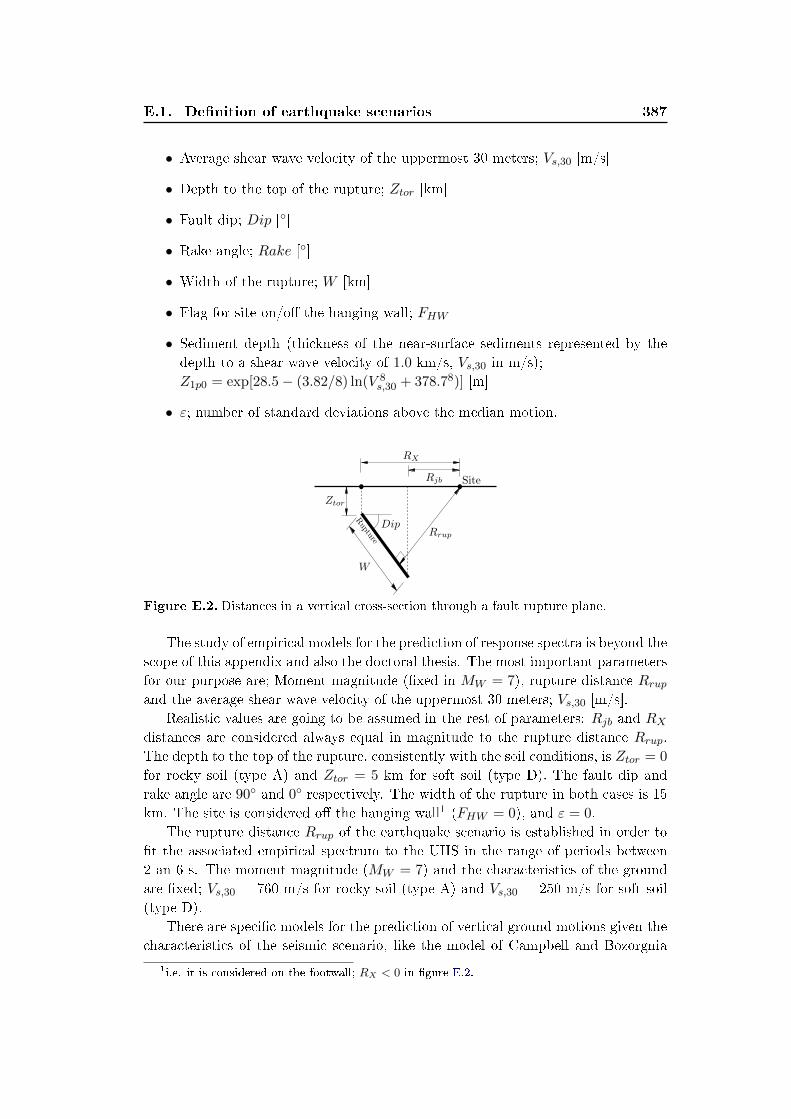
E.1. Denition of earthquake scenarios 387
• Average shear wave velocity of the uppermost 30 meters; Vs,30 [m/s]
• Depth to the top of the rupture; Ztor [km]
• Fault dip; Dip []
• Rake angle; Rake []
• Width of the rupture; W [km]
• Flag for site on/o the hanging wall; FHW
• Sediment depth (thickness of the near-surface sediments represented by thedepth to a shear wave velocity of 1.0 km/s, Vs,30 in m/s);Z1p0 = exp[28.5− (3.82/8) ln(V 8
s,30 + 378.78)] [m]
• ε; number of standard deviations above the median motion.
Figure E.2. Distances in a vertical cross-section through a fault rupture plane.
The study of empirical models for the prediction of response spectra is beyond thescope of this appendix and also the doctoral thesis. The most important parametersfor our purpose are; Moment magnitude (xed in MW = 7), rupture distance Rrupand the average shear wave velocity of the uppermost 30 meters; Vs,30 [m/s].
Realistic values are going to be assumed in the rest of parameters: Rjb and RXdistances are considered always equal in magnitude to the rupture distance Rrup.The depth to the top of the rupture, consistently with the soil conditions, is Ztor = 0
for rocky soil (type A) and Ztor = 5 km for soft soil (type D). The fault dip andrake angle are 90 and 0 respectively. The width of the rupture in both cases is 15km. The site is considered o the hanging wall1 (FHW = 0), and ε = 0.
The rupture distance Rrup of the earthquake scenario is established in order tot the associated empirical spectrum to the UHS in the range of periods between2 an 6 s. The moment magnitude (MW = 7) and the characteristics of the groundare xed; Vs,30 = 760 m/s for rocky soil (type A) and Vs,30 = 250 m/s for soft soil(type D).
There are specic models for the prediction of vertical ground motions given thecharacteristics of the seismic scenario, like the model of Campbell and Bozorgnia
1i.e. it is considered on the footwall; RX < 0 in gure E.2.
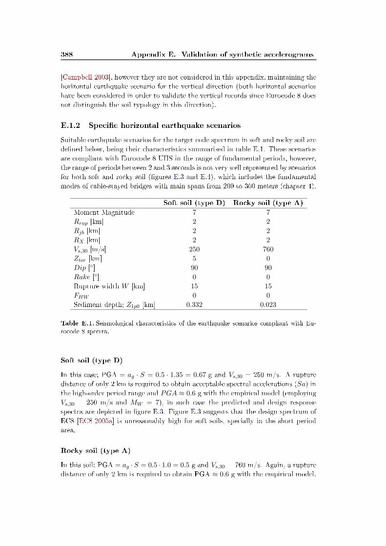
388 Appendix E. Validation of synthetic accelerograms
[Campbell 2003], however they are not considered in this appendix, maintaining thehorizontal earthquake scenario for the vertical direction (both horizontal scenarioshave been considered in order to validate the vertical records since Eurocode 8 doesnot distinguish the soil typology in this direction).
E.1.2 Specic horizontal earthquake scenarios
Suitable earthquake scenarios for the target code spectrum in soft and rocky soil aredened below, being their characteristics summarised in table E.1. These scenariosare compliant with Eurocode 8 UHS in the range of fundamental periods, however,the range of periods between 2 and 3 seconds is not very well represented by scenariosfor both soft and rocky soil (gures E.3 and E.4), which includes the fundamentalmodes of cable-stayed bridges with main spans from 200 to 300 meters (chapter 4).
Soft soil (type D) Rocky soil (type A)
Moment Magnitude 7 7
Rrup [km] 2 2
Rjb [km] 2 2
RX [km] 2 2
Vs,30 [m/s] 250 760
Ztor [km] 5 0
Dip [] 90 90
Rake [] 0 0
Rupture width W [km] 15 15
FHW 0 0
Sediment depth; Z1p0 [km] 0.332 0.023
Table E.1. Seismological characteristics of the earthquake scenarios compliant with Eu-
rocode 8 spectra.
Soft soil (type D)
In this case; PGA = ag · S = 0.5 · 1.35 = 0.67 g and Vs,30 = 250 m/s. A rupturedistance of only 2 km is required to obtain acceptable spectral accelerations (Sa) inthe high-order period range and PGA ≈ 0.6 g with the empirical model (employingVs,30 = 250 m/s and MW = 7), in such case the predicted and design responsespectra are depicted in gure E.3. Figure E.3 suggests that the design spectrum ofEC8 [EC8 2005a] is unreasonably high for soft soils, specially in the short periodarea.
Rocky soil (type A)
In this soil; PGA = ag · S = 0.5 · 1.0 = 0.5 g and Vs,30 = 760 m/s. Again, a rupturedistance of only 2 km is required to obtain PGA ≈ 0.6 g with the empirical model.

E.2. Seismological features 389
0 1 2 3 4 5 6 7Per iod; T [s]
0.0
0.2
0.4
0.6
0.8
1.0
1.2
1.4
1.6
1.8
Spec
tral
acce
lera
tion
;Sa
[g]
Engineers point of view
EC8 elast ic design spect rumEmpir ical model. Chiou and Youngs (2008)
10− 2 10− 1 100 101
Per iod; T [s]0.0
0.2
0.4
0.6
0.8
1.0
1.2
1.4
1.6
1.8
Spec
tral
acce
lera
tion
;Sa
[g]
Seismologists point of view
EC8 elast ic design spect rumEmpir ical model. Chiou and Youngs (2008)
Figure E.3. Eurocode 8 elastic design target spectrum and predicted spectrum (model of
Chiou and Youngs [Chiou 2008]). Soft soil (type D). Horizontal spectrum.
Both the predicted and the design response spectrum are represented in gure E.4.Unlike the result on soft soil, the t between the design spectrum and the empiricallypredicted one is adequate in a broad band of periods considering rocky soil; it mustbe recognized that most of the recorded accelerograms in PEER - NGA databasecorrespond to rocky soil conditions, and hence the empirical model of Chiou andYoungs may be more appropriate for these conditions. Furthermore, the Eurocode8 reference spectrum is precisely dened for rocky soil (TA).
0 1 2 3 4 5 6 7Per iod; T [s]
0.0
0.2
0.4
0.6
0.8
1.0
1.2
1.4
Spec
tral
acce
lera
tion
;Sa
[g]
Engineers point of view
EC8 elast ic design spect rumEmpir ical model. Chiou and Youngs (2008)
10− 2 10− 1 100 101
Per iod; T [s]0.0
0.2
0.4
0.6
0.8
1.0
1.2
1.4
Spec
tral
acce
lera
tion
;Sa
[g]
Seismologists point of view
EC8 elast ic design spect rumEmpir ical modelChiou and Youngs (2008)
Figure E.4. Eurocode 8 elastic design target spectrum and predicted spectrum (model of
Chiou and Youngs [Chiou 2008]). Rocky soil (type A). Horizontal spectrum.
E.2 Seismological features
The purpose of this section is to establish comparative features which are predictableby means of empirical expressions for real earthquakes based on the earthquake sce-narios dened above. These empirical models are not explained here, the interestedreader is directly referred to the relevant papers.

390 Appendix E. Validation of synthetic accelerograms
No distinctions are made by the authors of the predictive empirical models be-tween horizontal and vertical components, hence the models are considered appli-cable to both types of records.
In addition to the empirical predictions considered below, the qualitative aspectof the acceleration, velocity and displacement time histories have been contrastedwith El Centro (1940, MW = 7.1) benchmark record.
Peak Ground Acceleration (PGA)
As stated before, the earthquake scenario is established by matching the spectralacceleration of its empirical spectrum with the target code one in the long periodrange (2-6 s). Thus the PGA (spectral acceleration for a period equal to 0 s) isnot specically taken into account. However, PGA is an Intensity Measure (IM)historically considered in seismic studies, and here its simulated value with articialaccelerograms2 is compared with the predicted one adopting the empirical model ofChiou and Youngs [Chiou 2008].
Several researchers have demonstrated that PGA is an inecient Intensity Mea-sure, specially for exible structures like cable stayed bridges due to the greatinuence of the long period area of the spectrum, which is weakly correlated toPGA (this fact may be observed in gures E.3 and E.4).
Arias intensity
Arias Intensity (Ia, expression (5.1)) is an Intensity Measure (IM) that has beenproved to be more ecient than PGA for geotechnical considerations. Arias Inten-sity measures the strength of the accelerogram, and its prediction is establishedhere through the empirical model developed by Foulser Piggott and Staord[Foulser-Piggott 2010].
Duration of the strong pulse phase
The empirical model of Bommer et al [Bommer 2009] for the prediction of theSignicant Relative Duration (DSR) is employed in this appendix, which is validfor moment magnitudes between 4.8 and 7.9, and rupture distances up to 100 kmfrom the source, therefore it is valid for the earthquake scenarios considered (seetable E.1).
Husid plot
Husid plots study the rate of introduced seismic energy, being represented by theratio between the accumulated partial and total Arias Intensity versus the time
2Since synthetic accelerograms t the complete range of the target UHS, from 0.03 to 6.6 s(section 5.4.2), Sa(Tmin = 0.03) ≈ PGA, thus the simulated PGA with this articial accelerogramswill be approximately the value of ag employed to dene this design spectrum; PGA ≈ 0.5 g forhorizontal accelerograms in rocky soil (type A); and PGA ≈ 1.35 · 0.5 = 0.675 g for horizontalrecords in soft soil (type D).

E.3. Results 391
elapsed since the earthquake begins. It is clearly inuenced by the interval of strongshaking of the record; the longer this interval the more linear results the Husid plot.
The model of Staord et al [Staord 2009] is employed in order to predict theHusid plot produced by natural earthquakes.
E.3 Results
For the sake of brevity, only the comparison results are summarized here, collectingthe relevant conclusions at the end of the appendix. Two types of plots are presented;(i) the seismological features averaged from the considered set of 12 synthetic ac-celerograms, including not only the absolute values, but also their ratio with thepredicted ones based on natural records compliant with the specied seismic sce-narios; and (ii) the Husid plot with colour bands representing the relative durationDSR,5−75, comparing the articial results with the empirical model of Staord et al[Staord 2009].
In each case, the articial records obtained for Modal Response History Analysis(MRHA) and those obtained for Non-Linear Response History Analysis (NL-RHA)are distinguished, due to the dierences in their generation procedure (chapter 5).
Since the vertical spectrum in Eurocode 8 is independent of the type of foun-dation soil, the synthetic accelerograms obtained by tting this spectrum are com-pared with the empirical predictions for natural earthquakes compatible with bothhorizontal scenarios; only the comparison with the scenario in rocky soil (TA) arepresented for vertical records, the results are similar on soft soil.
In one of the studied cases, the results of Simqke [Gasparini 1999] have beenalso included, which is a well known software for the calculation of synthetic recordsfrom a specic target spectrum.
PGA [g] Ia [m/s] DSR,5−75[s] DSR,5−95[s]0
1
2
3
4
5
Sim
ulat
ed/P
redi
cted
0.6 2.6 5.0 11.60.7
10.4
8.3
13.80.7
11.8
10.3
14.1
MRHA accelerograms. Soil D
Predicted natural recordProposed in this thesis. SyntheticSimqke. Synthetic
(a) Earthquake features (b) Husid plot
Figure E.5. Horizontal records for soft soil (type D) employed in modal dynamics (MRHA).

392 Appendix E. Validation of synthetic accelerograms
PGA [g] Ia [m/s] DSR,5−75[s] DSR,5−95[s]0
1
2
3
4
5
Sim
ulat
ed/P
redi
cted
0.6 2.6 5.0 11.60.7
5.3
7.9
13.5
NL-RHA accelerograms. Soil D
Predicted natural recordPropoposed in this thesis. Synthetic
(a) Earthquake features
0 5 10 15 20Time; t [s]
0.0
0.2
0.4
0.6
0.8
1.0
Cum
ulat
ive
ener
gy/T
otal
ener
gy
Predicted natural record
Husid plot. NL-RHA. Soil D
Predicted
Synthetic
Proposed in this thesis. Synthetic
75 %
5 %
(b) Husid plot
Figure E.6. Horizontal records for soft soil (type D) employed in nonlinear dynamics (NL-
RHA).
PGA [g] Ia [m/s] DSR,5−75[s] DSR,5−95[s]0
1
2
3
4
5
Sim
ulat
ed/P
redi
cted
0.5 2.9 4.7 9.40.5
4.47.6
13.6
MRHA accelerograms. Soil A
Predicted natural recordProposed in this thesis. Synthetic
(a) Earthquake features
0 5 10 15 20Time; t [s]
0.0
0.2
0.4
0.6
0.8
1.0
Cum
ulat
ive
ener
gy/T
otal
ener
gy
Predicted natural record
Husid plot. MRHA accelerograms. Soil A
Proposed in this thesis. Synthetic
75 %
5 %
Synthetic
Predicted
(b) Husid plot
Figure E.7. Horizontal records for rocky soil (type A) and employed in modal dynamics
(MRHA).
PGA [g] Ia [m/s] DSR,5−75[s] DSR,5−95[s]0
1
2
3
4
5
Sim
ulat
ed/P
redi
cted
0.5 2.9 4.7 9.40.5 2.8
7.3 13.8
NL-RHA accelerograms. Soil A
Predicted natural recordProposed in this thesis. Synthetic
(a) Earthquake features
0 5 10 15 20Time; t [s]
0.0
0.2
0.4
0.6
0.8
1.0
Cum
ulat
ive
ener
gy/T
otal
ener
gy
Rocky soi l (type A)
Predicted natural record
Proposed. Synthetic
Husid plot. NL-RHA
Synthetic
Predicted75 %
5 %
(b) Husid plot
Figure E.8. Horizontal records for rocky soil (type A) and employed in nonlinear dynamics
(NL-RHA).
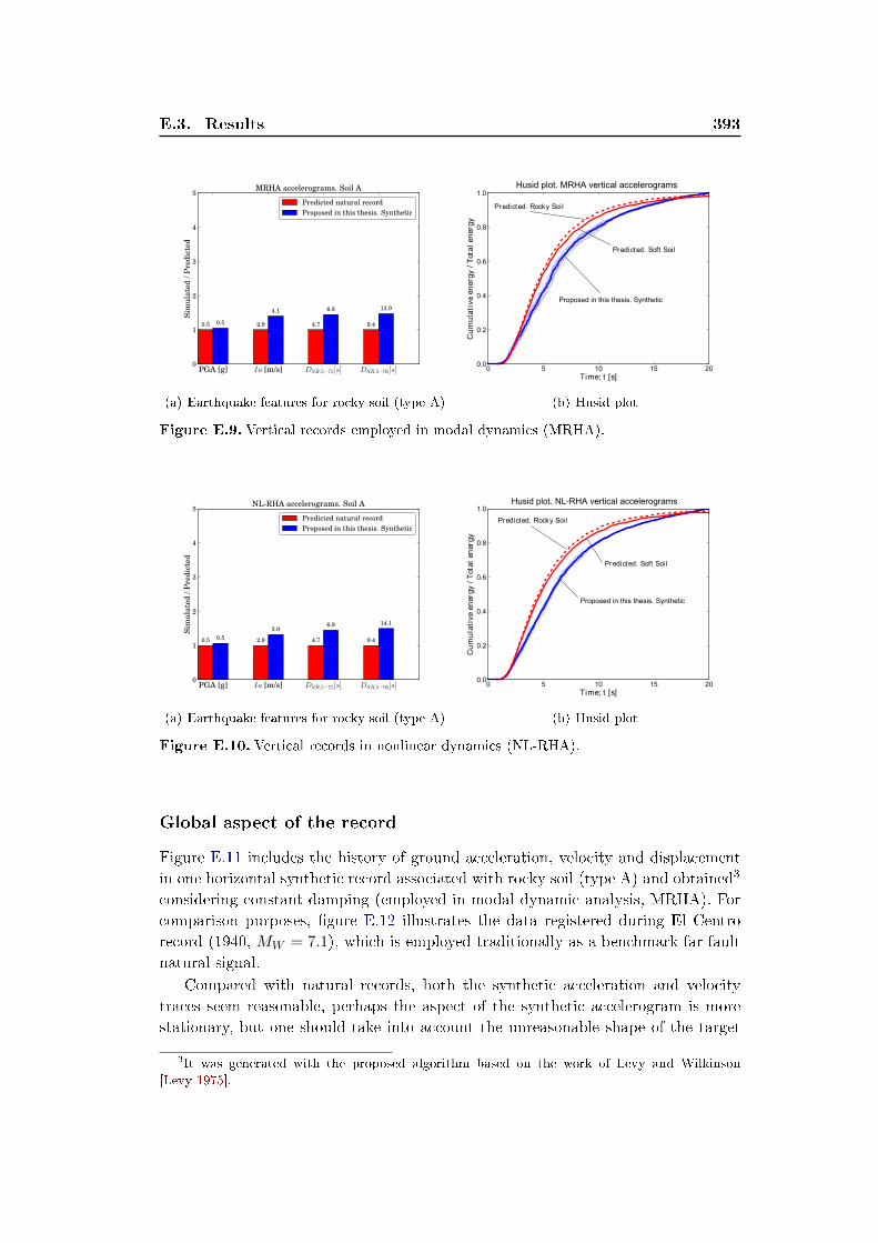
E.3. Results 393
PGA [g] Ia [m/s] DSR,5−75[s] DSR,5−95[s]0
1
2
3
4
5Si
mul
ated
/Pre
dict
ed
0.5 2.9 4.7 9.40.5
4.1 6.8 13.9
MRHA accelerograms. Soil A
Predicted natural recordProposed in this thesis. Synthetic
(a) Earthquake features for rocky soil (type A)
0 5 10 15 20Time; t [s]
0.0
0.2
0.4
0.6
0.8
1.0
Cum
ulat
ive
ener
gy/T
otal
ener
gy
Predicted. Soft Soi l
Predicted. Rocky Soil
Husid plot. MRHA vertical accelerograms
Proposed in this thesis. Synthetic
(b) Husid plot
Figure E.9. Vertical records employed in modal dynamics (MRHA).
PGA [g] Ia [m/s] DSR,5−75[s] DSR,5−95[s]0
1
2
3
4
5
Sim
ulat
ed/P
redi
cted
0.5 2.9 4.7 9.40.53.9
6.9 14.1
NL-RHA accelerograms. Soil A
Predicted natural recordProposed in this thesis. Synthetic
(a) Earthquake features for rocky soil (type A)
0 5 10 15 20Time; t [s]
0.0
0.2
0.4
0.6
0.8
1.0
Cum
ulat
ive
ener
gy/T
otal
ener
gy
Predicted. Soft Soi l
Predicted. Rocky Soil
Husid plot. NL-RHA vertical accelerograms
Proposed in this thesis. Synthetic
(b) Husid plot
Figure E.10. Vertical records in nonlinear dynamics (NL-RHA).
Global aspect of the record
Figure E.11 includes the history of ground acceleration, velocity and displacementin one horizontal synthetic record associated with rocky soil (type A) and obtained3
considering constant damping (employed in modal dynamic analysis, MRHA). Forcomparison purposes, gure E.12 illustrates the data registered during El Centrorecord (1940, MW = 7.1), which is employed traditionally as a benchmark far-faultnatural signal.
Compared with natural records, both the synthetic acceleration and velocitytraces seem reasonable, perhaps the aspect of the synthetic accelerogram is morestationary, but one should take into account the unreasonable shape of the target
3It was generated with the proposed algorithm based on the work of Levy and Wilkinson[Levy 1975].
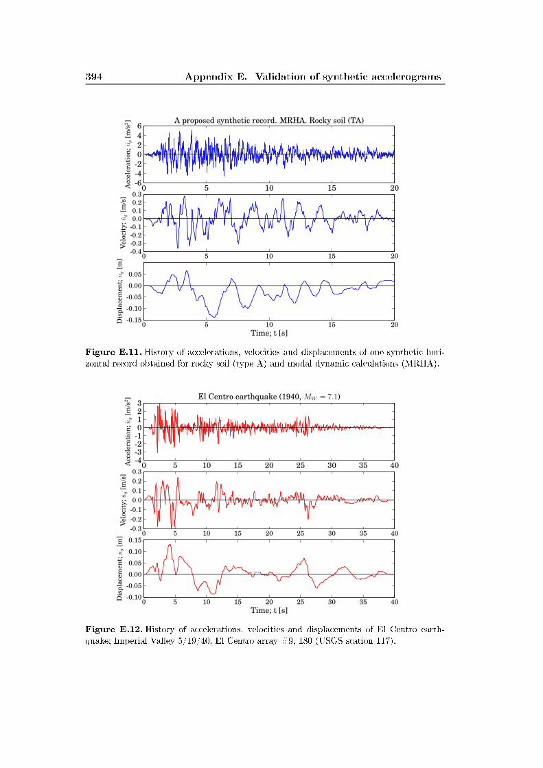
394 Appendix E. Validation of synthetic accelerograms
0 5 10 15 20-6-4-20246
Acc
eler
atio
n;ug
[m/s
2] A proposed synthetic record. MRHA. Rocky soil (TA)
0 5 10 15 20-0.4-0.3-0.2-0.10.00.10.20.3
Vel
ocit
y;ug
[m/s
]
0 5 10 15 20Time; t [s]
-0.15
-0.10
-0.05
0.00
0.05
Dis
plac
emen
t;ug
[m]
Figure E.11. History of accelerations, velocities and displacements of one synthetic hori-
zontal record obtained for rocky soil (type A) and modal dynamic calculations (MRHA).
0 5 10 15 20 25 30 35 40-4-3-2-10123
Acc
eler
atio
n;ug
[m/s
2] El Centro earthquake (1940, MW = 7.1)
0 5 10 15 20 25 30 35 40-0.3-0.2-0.10.00.10.20.3
Vel
ocit
y;ug
[m/s
]
0 5 10 15 20 25 30 35 40Time; t [s]
-0.10
-0.05
0.00
0.05
0.10
0.15
Dis
plac
emen
t;ug
[m]
Figure E.12. History of accelerations, velocities and displacements of El Centro earth-
quake; Imperial Valley 5/19/40, El Centro array #9, 180 (USGS station 117).

E.4. Conclusions 395
spectrum imposed to the articial record. Associated with the accelerograms ob-tained for soft soil conditions (TD), there is an appreciable baseline drift at the endof the displacement history; in principle this permanent movement is harmless sinceit leads to rigid body motions in the structure. The proposed algorithm may be eas-ily corrected to overcome this unrealistic feature, but it has been veried elsewherethat the eect is not important for the extreme seismic response [Abaqus 2010], andno attempt has been made to reduce the baseline drift in the proposed syntheticrecords.
E.4 Conclusions
Keeping in mind that the predicted natural spectrum, associated with a realistic seis-mic scenario, cannot be matched to the UHS provided by design codes in the wholerange of interesting periods, and assuming the inherent errors in empirical models,the following conclusions arise from the comparison between articial records andempirical predictions based on natural earthquakes:
• The modied proposal of Levy & Wilkinson [Levy 1975] algorithm to obtainthe synthetic accelerograms employed in this thesis, yields records closer tothe predicted natural ones in comparison with Simqke [Gasparini 1999] results,in terms of Arias Intensity, Signicant Durations, rate of introduction of theenergy during the seismic excitation and global aspect of the accelerogram(which are less stationary). This is probably due to the possibility of reducingeasily the strong pulse interval (tsp) in the proposed algorithm, getting closerto the natural results.
• The total amount of energy (Arias Intensity) introduced by natural predictedearthquakes is generally lower than the one associated with articial records,which is specially true in soft soil scenarios, where material nonlinearities areexpected to be strong in exible structures like cable-stayed bridges.
• The envelope modulating function of maximum accelerations F (t), which isstrongly related to signicant durations (veried here), has been obtained fromthe recommendations of Priestley [Priestley 1996] and Eurocode 8 [EC8 1994].Nevertheless, simulated signicant durations are larger than the predicted val-ues for coherent natural records, and therefore, the rate of introduction of theenergy (Husid plot) is lower for synthetic accelerograms.
• The special procedure employed to obtain synthetic accelerograms appropriatefor nonlinear dynamics (with Rayleigh damping) leads to more realistic AriasIntensities in such records. Hence, articial accelerograms closer to the naturalones are obtained in nonlinear calculations, which could be sensitive to thisfeature (elastic modal dynamics is independent of the energy content, durationand other accelerogram characteristics, the most important feature in elasticanalysis is indeed the t of the spectrum).

396 Appendix E. Validation of synthetic accelerograms
• The overestimation in the Arias Intensity using articial accelerograms is dueto unrealistically large durations of the strong pulse interval, which is di-rectly related to the signicant duration DSR,5−75. An easy way to solvethis problem, obtaining more realistic synthetic accelerograms, is to modifythe modulating function F (t) (presented in gure 5.3) by reducing the strongshaking interval (tsp), resulting Husid plots more consistent with the naturalprevisions4. However, this implies a deviation from the recommendations ofEurocode 8 [EC8 1994]. Such procedure is not further developed here, adopt-ing the normative modulating function, which is supported by the results ofprevious research works [Jangid 2004] [Quek 1990].
• The Peak Ground Acceleration (PGA) obtained in the synthetic records is veryclose to the expected value (with variations between ±10 %); PGA = 0.5 · Sg, where S = 1 for rocky soil and S = 1.35 for soft soil, whereas in thevertical accelerograms PGAV = 0.9 · PGAH = 0.45 g. The predicted PGA innatural records is somewhat dierent, because the imposed t of the empiricalspectra to the design one is done mainly in the range of long periods, whilst noconstraint is imposed in the area of high frequencies, where PGA is stronglycorrelated.
• The vertical synthetic accelerograms are observed to follow the same trendsthan horizontal ones associated with rocky soil, due to the good agreementwith Eurocode 8 spectra, presenting Arias Intensity close to the predictions.
• The frequency of the strong acceleration pulses is larger for rocky soil, becausethe horizontal target spectrum associated with this ground gives more promi-nence to spectral accelerations in the high frequency range than the spectrumin soft soil (see gure 5.1). The spectrum shape also explains the large containof strong pulses in vertical synthetic records.
4There are other more comprehensive proposed envelope modulating functions F (t), like themodel of Staord et al (2009) [Staord 2009] (the Husid plot recommended by these authors hasbeen considered in the present appendix). Nevertheless, the denition of earthquake scenarios isrequired to dene DSR,5−75, reducing the generality of the study.

Appendix F
Pushover analysis in seismic codes
and guidelines
The objective of code-compliant pushover analysis is to reduce the structure to aninelastic SDOF system properly dened, and usually related to the fundamentalvibration mode.
F.1 Eurocode 8 - Part 2: Bridges
Following Eurocode 8 (Part 2) [EC8 2005a], pushover is performed separately inboth longitudinal and transverse directions. The investigation of two pattern loadsis recommended;
• Triangular: The displacement at the level of the deck is assumed constantand piers are subjected to linearly increasing loads from the foundation totheir top:
s∗i = mi ·ziHtot
(F.1)
Where s∗i , mi and zi are respectively the load, mass and height associatedwith node i, whilst Htot is the height of the pier.
• Principal Mode: The load pattern is proportional to the principal modein each direction, which is considered the one with the highest correspondingparticipation factor Γ:
s∗i = mi · φi,p (F.2)
Where φi,p is the modal displacement at node i in the principal mode.
The target inelastic displacement demand of the equivalent SDOF (um) is con-sidered equal to the elastic displacement of the centre of mass of the deformed deck(control point) when linear multi-mode spectrum analysis is performed1, tacitly
1According to Eurocode 8 (Part 2) [EC8 2005a], the target displacement is considered equal tothe maximum displacement obtained between two seismic elastic combinations; (1) longitudinalearthquake spectrum combined with 30 % of the transverse spectrum and (2) transverse earthquakespectrum combined with 30 % of the longitudinal spectrum.

398 Appendix F. Pushover analysis in seismic codes and guidelines
considering that bridges are exible enough to apply the `equal deformation' rule(um ≈ uo, see gure F.1), which is reasonable for vibration periods in the velocity-and displacement-sensitive regions of the spectrum, i.e T > TC s 2. This rule maybe deemed appropriate in cable-stayed bridges due to their important exibility,nevertheless, it has been veried in the present work that several inuencing lon-gitudinal or transverse modes could be located in the acceleration-sensitive regionof the spectrum, specially if the foundation soil is soft3, and therefore the `equaldeformation' rule should be questioned.
Eurocode 8 (Part 1) [EC8 2004] is prepared for this situation (when relativelysti modes inuence the response) and provides a simplied expression to estimatethe inelastic target displacement of such periods (where T <= TC):
um ≈uoqu
[1 + (qu − 1)
TCT
]≥ uo; if T ≤ TC
um ≈ uo; if T > TC
(F.3)
uo = Sd(T, ξ) being the peak displacement obtained by considering the initialelastic SDOF properties (see gure F.1) and T the vibration period of this elasticresponse, whereas qu is the ratio between the acceleration in the elastic equivalentproblem (Sa(T, ξ)) and the inelastic SDOF system (Fy/Meff , where Meff is themass of the SDOF4 and Fy its elastic limit); hence qu = Sa(T, ξ)Meff/Fy. Finally,TC is the aforementioned corner frequency.
Figure F.1. Elastoplastic system and its corresponding linearization.
2Following Eurocode 8 [EC8 2005a], in rocky soil class (TA) TC = 0.4 s, whereas in soft soilclass (TD) TC = 0.8 s.
3Table 6.1 includes the governing frequencies of several cable-stayed bridges on soft soil, andthere may be appreciated that models with 200 m main span could be dominated by periods lowerthan TC = 0.8 s (TD), i.e. frequencies higher than f = 1.25 Hz.
4Meff is the eective mass of the studied mode, obtained with eq. (4.3).

F.2. ATC-40 399
Anyhow, Eurocode 8 (Part 2) [EC8 2005a] discourages pushover analysis if themass of some piers has a signicant eect on its dynamic behaviour, which is clearlythe case in cable-stayed bridges due to the large mass of the towers, recommendingnonlinear dynamics (NL-RHA) in such cases.
F.2 ATC-40
ATC-40 [ATC 1996] was one of the rst guidelines proposing pushover as a method-ology to study the nonlinear seismic behaviour of buildings. The load pattern pro-posed in ATC-40 is the `Principal Mode' described above.
The inelastic target displacement is estimated by means of an iterative pro-cedure called `capacity-spectrum' method, where a sequence of elastic SDOF areanalyzed by updating the period and equivalent damping ratio5. This proceduredoes not always obtain convergence, and when it does converge, the solution couldbe misleading [Chopra 2007]. The pushover analysis leads to the capacity curve,which is expressed in ADRS coordinates6. The reduced spectra, taking into accounthysteretic damping by means of simplied rules focused on building structures, isrepresented along with this plot. The reduction of the spectrum due to such equiv-alent viscous damping (ξ) may be done by using the reduction factor proposed byseismic codes (for example η =
√10/(5 + ξ) ≥ 0.55 is proposed by Eurocode 8
[EC8 2004]), which is known to present lack of physical basis.Shortcomings of ATC-40 methodology in the estimation of the inelastic displace-
ment demand appear to have been rectied in FEMA-440 report [fem 2005], but thebenets in the equivalent linearization detour is unclear when there are available ex-pressions for the inelastic deformation ratio, like the one proposed by Eurocode 8and presented in equation (F.3) [Chopra 2007].
ATC-40 suggests the possibility of including higher mode eect for high-risebuildings with fundamental period larger than 1 s, which are observed to be the mostsensitive to such modes, by repeating the `capacity-spectrum' method for importantmodes dierent than the rst one.
F.3 FEMA-356
FEMA-356 [fem 2000] is a seismic guideline focused on building structures. Atleast two load distribution patterns must be considered separately and the mostdemanding results are selected. The rst load distribution is to be selected fromamong the following:
• Principal Mode
• Equivalent Lateral Force (ELF), analogous to triangular distribution.
5The `capacity spectrum' procedure has been described by the author elsewhere [Camara 2008].6ADRS coordinates represent a plot of spectral displacements (horizontal axis) versus spectral
accelerations (vertical axis).

400 Appendix F. Pushover analysis in seismic codes and guidelines
• MRSA pattern: s∗ is dened with the storey shears obtained from the elasticspectrum analysis (MRSA) of the structure.
The second pattern is either the `Uniform' distribution (where the load is equalto the mass associated with each point, s∗i = mi) or an adaptive one which variesas the structure yields. There are many research works available in literature aboutthe applicability of these load patterns to building structures, several concludingthat `Uniform' distribution is not appropriate since it grossly underestimates thedrifts in upper stories, and overestimates them in lower stories [Chopra 2007]. Inthe present work `Principal Mode' and `Uniform' patterns were studied in severalcable-stayed bridges and `Uniform' distribution is also found to yield wrong results(see section 6.4.4.2).
The target displacement of the SDOF system is estimated by means of the`coecient method':
um = C1C2C3
(T
2π
)2
Sa︸ ︷︷ ︸Sd
(F.4)
Where the elastic spectral displacement of the considered vibration mode (Sd) isincreased by three coecients; C1 represents the inelastic deformation ratio um/uo(again, um is the maximum inelastic displacement and uo is the maximum displace-ment of the equivalent elastic SDOF, see gure F.1) for SDOF systems with stablehysteresis loops (i.e. without stiness degradation, pinching, etc.), the coecientC2 considers the increase in the deformation due to the damage eects which arenot covered in C1, whereas C3 takes into account the increase in the deformationbecause of the negative post-yielding stiness arising from P-∆ eects. The princi-pal problem is that values provided for such coecients are not prepared to be usedin bridges, and some numerical results are not supported by research [Chopra 2007].Improvements in coecients C1 and C2 were established in FEMA-440 [fem 2005]report.
If higher modes are important in the response of the structure, pushover issupplemented by the linear dynamic analysis according to FEMA-356.

Appendix G
Step-by-step description of
advanced pushover analysis
The advanced pushover analysis (NSP) employed in this thesis, and presented inchapter 6, are detailed here in step-by-step form; Modal Pushover Analysis (MPA)was proposed by Chopra and Goel [Chopra 2002] and is widely accepted in buildingstructures, several contributions have been devised to adapt the methodology tothe three-directional seismic response of cable-stayed bridges; The Extended ModalPushover Analysis (EMPA) is a generalization of MPA suggested to fully considerthe three-axial ground motions; and the Coupled Nonlinear Static Pushover (CNSP)is a procedure developed here to take into account the nonlinear couplings betweengoverning transverse and longitudinal modes.
The procedures are presented in a general form and could be applied to anystructure.
G.1 Modal Pushover Analysis: MPA
1. Apply rst the gravity loads considering geometric nonlinearities (P-∆ eects).
2. Perform modal analysis from the deformed conguration of the structure, com-puting frequencies fn, participation factors Γjn (j = X,Y, Z) and mode shapesφn up to the maximum frequency of interest; fmax = 25 Hz. After the modalanalysis, a study about the participation of each mode below fmax in the globalresponse in terms of forces or displacements should be conducted (see section6.4.4.1), identifying the governing longitudinal (fnX) and transverse modes(fnY ), MPA should involve both dominant modes. The limit frequency whichmarks the end of the range where pushover is to be conducted is establishedas fgov = max(fnX , fnY ).
3. For the modes below the limit fgov, their dominant direction (DRn) is se-lected because MPA does not consider the three-directional contribution ofmodes, and subsequently the analysis continues in 2D (either longitudinally,transversely or vertically, depending on the governing direction of the specicmode). The control point is selected for each vibration mode as the node withmaximum modal displacement in the dominant direction. A proposed methodto obtain the characteristic direction of the mode is presented in section 6.4.4.1,summarized in the expression below.

402 Appendix G. Step-by-step description of advanced pushover
ΓDRn = maxj
(Γjn)
; with j = X,Y, Z → DRn (G.1)
4. For the nth mode, within the range studied by pushover analysis (fn ≤ fgov),develop the base shear versus control point displacement curve in the dominantdirection, Vbn − urn, by means of nonlinear static analysis (pushover) of thestructure when the load distribution s∗n = mφn is incrementally applied (self-weight included), ignoring the components in the direction dierent than thedominating one. The base shear (Vbn) is the sum of the shear recorded ineach foundation (towers, intermediate piers and abutments) in the dominantdirection of the mode, and the control point displacement urn is consequentlythe displacement of this point along the dominant direction in the nth mode(it position depends on the vibration mode).
5. Transform Vbn−urn pushover curve to Fsn/Mn− qn coordinates using expres-sions (6.37a) and (6.37b), repeated here for convenience:
FsnMn
=VbnLn
(G.2a)
qn =urnφrn
(G.2b)
6. Idealize the real Fsn/Mn−qn curve for the equivalent SDOF system associatedwith nth mode. Here, a bi-linear curve considering a modied `Equal Area' rulepresented in gure 6.11(a) (section 6.4.1) is proposed because of its simplicity,but more realistic curves may be considered. The kinematic properties of thenonlinear spring behaviour in the SDOF system need to be addressed (seeappendix H), dening the loading and unloading branches appropriate for thestructural system and material.
7. Compute the peak generalized displacement qn of the n-mode inelastic SDOFsystem1. Here, it is proposed to integrate the SDOF dierential equation ofthe corresponding mode in time domain (repeated below), by implementingthe algorithm presented in appendix H.
qn + 2ξnωnqn +FsnMn
= −Γnug (G.3)
8. Obtain the peak control point displacement urn with expression: urn = qnφrn,where φrn is the modal displacement in the dominant directionDRn of n-modeat the selected control point.
1Dierent options are available in the literature in order to obtain the target control pointdisplacement in pushover analysis, some of them have been presented in appendix F.

G.2. Extended Modal Pushover Analysis: EMPA 403
9. Interpolate with urn + uG (being uG the control point displacement in thedominant direction due to gravity loads) from the database of pushover anal-ysis, to obtain the combined eects of lateral loads and gravity due to n-modecontribution (rn+G).
10. Obtain the contribution of n-mode to the seismic response exclusively, byextracting the eect due to the self-weight: rn = rn+G − rG, where rG is thecontribution considering the self-weight acting alone.
11. Repeat steps 4 to 10 for all modes with frequencies below or equal fgov.
12. Obtain the total nonlinear seismic response by combining the contribution ofeach mode with frequency below fgov, using an appropriate combination rule,here CQC rule is selected for this purpose: rnl.
13. Compute the higher mode seismic response (rel) by means of spectrum analysis(MRSA) including modes with frequencies higher than fgov and lower or equalthan fmax = 25 Hz.
14. Combine the participation of rst modes with the higher mode eect (betweenfgov and fmax), employing SRSS combination rule to obtain the dynamic re-
sponse of the structure: rd ≈√r2nl + r2
el. Frequencies higher than fmax = 25
Hz are ignored.
15. Calculate the total demand (r) by combining the self-weight eect (rG) withthe dynamic contribution exclusively due to the earthquake (rd). Since thesign of seismic forces is lost in pushover procedures2, two hypotheses are made,considering both positive and negative signs in the earthquake response to takeinto account that the seismic input, and the consequent structural behaviour,have alternating sign reversals.
r ≈ max (rG ± rd) (G.4)
G.2 Extended Modal Pushover Analysis: EMPA
EMPA proposed procedure is summarized next, repeating for completeness somesteps introduced in MPA:
1. Apply rst the gravity loads considering geometric nonlinearities (P-∆ eects).
2. Perform modal analysis from the deformed conguration of the structure, com-puting frequencies fn, participation factors Γjn (j = X,Y, Z) and mode shapesφn up to the maximum limiting frequency; fmax = 25 Hz. Next, a studyabout the participation of each mode below fmax in the global response in
2Pushover is equivalent to spectrum analysis in the elastic range.

404 Appendix G. Step-by-step description of advanced pushover
terms of forces or displacements is conducted (see section 6.4.4.1), identifyingthe governing longitudinal (fnX) and transverse modes (fnY ), EMPA coversboth dominant modes. The limit frequency which marks the end of the rangewhere pushover is to be conducted is established as fgov = max(fnX , fnY ).
3. For the nth mode, included in the range studied by pushover analysis (fn ≤fgov), develop the base shear-control point displacement curve, Vbn− urn 3, bymeans of three-dimensional nonlinear static analysis of the structure when theload distribution s∗n = mφn is incrementally applied (self-weight included),now fully considering its three-dimensional characteristics. Three pushovercurves are obtained while the structure is being pushed beyond the linearrange, each one associated with the longitudinal, transverse and vertical di-rections; (V X
bn −uXrn), (V Ybn−uYrn) ,(V Z
bn−uZrn) (see gure 6.14). The base shearV jbn is the sum of the shear recorded in each connection of the model to the
ground in j-direction during the pushover analysis of nth mode, whilst thecontrol point displacement ujrn is consequently the displacement of the controlpoint in j-direction; this point, is selected as the node with maximum modaldisplacement regardless of the direction where it is recorded.
4. Transform each V jbn − u
jrn pushover curves to F jsn/Mn − qjn coordinates using
expressions (6.46) and (6.47), repeated below:
F jsnMn
=V jbn
Ljn; with j = X,Y, Z (G.5)
qjn =ujrn
φjrn; with j = X,Y, Z (G.6)
5. Idealize the real F jsn/Mn − qjn curve for the equivalent SDOF system associ-ated with n-mode in j-direction. Here, a bi-linear curve considering a modied`Equal Area' rule presented in gure 6.11(a) is proposed because of its sim-plicity (more realistic curves could be considered). The kinematic propertiesof the nonlinear spring behaviour in the SDOF system need to be addressed(see appendix H), dening the loading and unloading branches appropriate forthe structural system and material.
6. Obtain a modular Fsn/Mn − qn from the three-directional results using ex-pressions (6.48) and (6.49), repeated next:
FsnMn
=
√(FXsnMn
)2
+
(F YsnMn
)2
+
(FZsnMn
)2
(G.7)
qn =
√(qXn )2 + (qYn )2 + (qZn )2 (G.8)
3The bar symbol means `magnitude' of the three directional displacement or shear components.

G.2. Extended Modal Pushover Analysis: EMPA 405
7. Compute the peak generalized modular displacement qn of the n-mode in-elastic SDOF system. Here, the integration of the SDOF dierential equation(6.45) of the corresponding mode in time domain (repeated below) is proposed,following the scheme presented in appendix H.
¨qn + 2ξnωn ˙qn +FsnMn
= −u∗g,n (t) (G.9)
Where u∗g,n (t) = ΓXn uXg (t) + ΓYn u
Yg (t) + ΓZn u
Zg (t), and ujg the accelerogram
3D components.
8. Obtain the peak modular control point displacement urn with:
umaxrn = φrn max
t[qn (t)] (G.10)
9. Interpolate with urn+uG (being uG the modular displacement of control point
due to gravity loads; uG =√
(uXG )2 + (uYG)2 + (uZG)2) from the database of thethree-dimensional pushover analysis, in order to obtain the combined eectsof lateral loads and gravity due to n-mode contribution rn+G.
10. Obtain the contribution of n-mode to the seismic response exclusively, byextracting the eect due to the self-weight: rn = rn+G − rG, where rG is thecontribution of gravity loads acting alone.
11. Repeat steps 3 to 10 for all modes with frequencies below or equal fgov.
12. Obtain the total nonlinear seismic response (rnl) by combining the contribu-tion of each studied mode using an appropriate combination rule, here CQCrule is selected for this purpose.
13. Compute the higher mode seismic response (rel) by means of spectrum analysis(MRSA), including modes with frequencies higher than fgov and lower or equalthan fmax = 25 Hz.
14. Combine the participation of rst modes with the higher mode eect by meansof SRSS combination rule to obtain the dynamic response of the structure:
rd ≈√r2nl + r2
el.
15. Calculate the total demand by combining the eect due to self-weight (rG)with the dynamic contribution due to the earthquake exclusively (rd). Sincethe sign of earthquake forces is lost in pushover procedures, two hypotheses aremade, considering both positive and negative signs in the earthquake response,which takes into account the alternating nature of the seismic response.
r ≈ max (rG ± rd) (G.11)

406 Appendix G. Step-by-step description of advanced pushover
G.3 Coupled Nonlinear Pushover Analysis: CNSP
The steps involved in the proposed coupled pushover (CNSP) are detailed next,repeating for convenience several features introduced in MPA and EMPA:
1. Apply rst the gravity loads considering geometric nonlinearities (P-∆ eects).
2. Perform modal analysis from the deformed conguration of the structure, com-puting frequencies fn, participation factors Γjn (j = X,Y, Z) and mode shapesφn up to the limit maximum frequency fmax = 25 Hz. Next, a study aboutthe participation of each mode below fmax in the global response in termsof forces or displacements is conducted (see section 6.4.4.1), identifying thegoverning4 longitudinal (fnX) and transverse (fnY ) frequencies.
3. Expand the excitation vector of the dominant longitudinal (nX) and trans-verse (nY ) modes, and compute the weight of dominant nk-mode in directionj (αjnk) by adding its expanded nodal forces (sjnk,i in node i) along the wholestructure (k = X,Y and j = X,Y, Z). Alternatively, the ratio could be mod-ied substituting the summations by the corresponding participation factors.
αjnk =
Nnode∑i=1
sjnk,i
Nnode∑i=1
sjnX,i +Nnode∑i=1
sjnY,i
(G.12)
4. Considering the two dominant longitudinal (nX) and transverse (nY ) modes,develop the base shear versus control point displacement curve, ¯VbC − ¯urC , bymeans of 3D nonlinear static analysis of the structure (self-weight included),incrementally increasing the coupled load pattern s∗C of expression (6.52) (con-sidering the fully 3D characteristics of the excitation vector s∗n):
s∗C = ΛY s∗nY + ΛXs
∗nX (G.13)
Λj = Saj/max(SaY , SaX), where Saj is the spectral acceleration associatedwith the governing mode in j-direction5, k = X,Y .
The displacement is measured simultaneously in two points during the cou-pled pushover, corresponding to the control points of the longitudinal andtransverse governing modes (selected according to EMPA described above).
4CNSP, unlike MPA and EMPA, only conducts one pushover analysis using a combination ofloads from the transverse and longitudinal governing modes, instead of performing nonlinear staticanalysis for all the modes with frequencies below or equal to fgov = max(fnX , fnY ).
5The component in j-direction of the coupled excitation vector (s∗ jC ) is obtained by consideringthe corresponding Λ applied to this direction, i.e. by selecting the acceleration spectrum in directionj when expression (6.53) is applied (if j = X,Y the spectrum is horizontal, if j = Z is the verticaldesign one).

G.3. Coupled Nonlinear Pushover Analysis: CNSP 407
5. The contributions of each dominant vibration mode to the longitudinal andtransverse projections of the coupled capacity pushover curve, are computedby multiplying the projection in j-direction (V j
bC − ujrC) by the weight factor
αjnX or αjnY expressed above. Three pushover curves are obtained per bothtwo dominant modes; (V j
bnX − ujrnX) and (V jbnY − ujrnY ) with j = X,Y, Z
(see gure 6.15). The base shear V jbnX and V j
bnY is respectively the sum ofthe shear recorded in each foundation of the model in the j-direction of eachdominant mode, whilst the control point displacement ujrnX and ujrnY is, con-sequently, the displacement in the j-direction for each governing longitudinaland transverse mode at the corresponding control point in a respective way.
6. Transform each V jbnX − u
jrnX and V j
bnY − ujrnY pushover curves respectively
into F jsnX/Mn − qjnX and F jsnY /Mn − qjnY coordinates by means of:
F jsnkMnk
=V jbnk
Ljnk; with j = X,Y, Z and k = X,Y (G.14)
qjnk =ujrnkφjrnk
; with j = X,Y, Z and k = X,Y (G.15)
7. Idealize the real F jsnX/MnX−qjnX and F jsnY /MnY −qjnY curves for the equiva-lent SDOF systems associated with each governing mode in j-direction. Here,it is proposed to use a bi-linear curve considering a modied `Equal Area' rulepresented in gure 6.11(a) (more realistic curves may be considered). Thekinematic properties of the nonlinear spring behaviour in the SDOF systemneed to be simulated (see appendix H), dening the loading and unloadingbranches appropriate for the structural system and material.
8. Obtain modular FsnX/MnX − qnX and FsnY /MnY − qnY relations from thedirectional results using expressions (k = X,Y ):
FsnkMnk
=
√(FXsnkMnk
)2
+
(F YsnkMnk
)2
+
(FZsnkMnk
)2
(G.16)
qnk =
√(qXnk)2
+(qYnk)2
+(qZnk)2
(G.17)
9. Compute the peak generalized modular displacements qnX of the governinglongitudinal nX-mode inelastic SDOF system, and analogously for the dom-inant transverse nY -mode the peak qnY . Here, integrating the dierentialequation (6.45) of the corresponding governing mode in time domain (repeatedbelow for nk-mode) is proposed, following the algorithm in appendix H.
¨qnk + 2ξnkωnk ˙qnk +FsnkMnk
= −u∗g,nk (t) (G.18)

408 Appendix G. Step-by-step description of advanced pushover
10. Obtain the peak modular control point displacements of the governing modes;urnX and urnY respectively, with expressions urnX = φrnX max
t[qnX (t)] and
urnY = φrnY maxt
[qnY (t)], where φrnX and φrnY are the modular modal dis-
placements at control point in longitudinal and transverse dominating modesrespectively.
11. Interpolate with urnX + uG (being uG the modular displacement of control
point due to gravity loads: uG =√
(uXG )2 + (uYG)2 + (uZG)2) from the databaseof three-dimensional pushover analysis particularized for the longitudinal gov-erning mode (VbnX − urnX), to obtain the combined eects of lateral loadsand gravity due to nX-mode contribution; rnX+G. Analogously, the contribu-tion of the governing transverse mode nY , rnY+G, is obtained by interpolatingurnY + uG in the pushover curve (VbnY − urnY ).
12. Obtain the contribution of nX-mode and nY -mode to seismic response ex-clusively, by extracting the eect due to self-weight: rnX = rnX+G − rG andrnY = rnY+G − rG, where rG is the contribution of gravity loads alone.
13. Combine the three-dimensional contributions of governing nX-mode and nY -mode through the CQC combination rule, obtaining rnl.
14. Compute the contributions of vibration modes dierent than the governingones and below fmax = 25 Hz, assuming their response elastic (rel). Thiselastic eect is obtained by means of spectrum analysis (MRSA). Vibrationmodes above 25 Hz are neglected.
15. Combine through SRSS rule the contribution of governing modes with thecontribution of modes below 25 Hz and dierent than the governing ones, in
order to obtain the dynamic response of the structure: rd ≈√r2nl + r2
el.
16. Calculate the total demand by combining the self-weight eect rG with thedynamic contribution due to the earthquake exclusively rd. Since the signof earthquake forces is lost in pushover procedures, two hypotheses are made(taking into account the alternating nature of the seismic input), consideringboth positive and negative signs in the earthquake response.
r ≈ max (rG ± rd) (G.19)

Appendix H
Nonlinear SDOF: description and
integration
In this appendix, the algorithm proposed by Simo and Hughes [Simo 1998] to in-tegrate a nonlinear SDOF system with combined isotropic/kinematic hardening isdescribed, which has been implemented in Matlab [Matlab 2011]. This algorithm isinvolved in advanced pushover procedures detailed in chapter 6 and appendix G.
We consider now the nonlinear SDOF represented by a unit-length element withelastic and frictional behaviour. Figure H.1 presents the schematic constitutivemodel of a nonlinear SDOF system with yielding stress σY . Two extreme cases ofthe hardening rule may be considered; the isotropic hardening assumes the yield sur-face only able to expand itself, with its center xed along the time; the kinematichardening, however, considers the movement of the yield surface in the directionof the plastic ow, maintaining constant its dimensions (Bauschinger eect). Thecyclic behaviour of real metals is somewhere in the middle of such extreme idealizedresponses, which is taken into account in the combined isotropic/kinematic harden-ing (Simo and Hughes [Simo 1998]). The failure criterion describing the solution insuch case is:
f(σ, q, α) := |σ − q| − (σY +Kpα) ≤ 0 (H.1)
q being the back stress, its evolution is dened by Ziegler's rule as:
q = Hεp ≡ γHsign(σ − q) (H.2)
Where H is the kinematic hardening modulus, εp is the plastic strain rate, γ ≥ 0
is the rate at which slip takes place and α is a `nonnegative function' of the amountof plastic ow (slip) called internal hardening variable, being its evolution denedin a simplied way by α = γ.
Figure H.1. Constitutive characterization of the nonlinear SDOF.
410 Appendix H. Nonlinear SDOF integration
To address the numerical implementation of the cyclic loading in the nonlin-ear SDOF, the auxiliary variable called relative stress; ζ := σ − q is dened forconvenience in algorithm 1.
In algorithm 1, E is the elasticity modulus of the element representing the elasticstiness of the nonlinear SDOF system, and Kp is the plastic modulus (slope of thehardening response in the space of plastic deformations σ − εp). The elastoplastictangent modulus (slope of the hardening response in the space of total deformationsσ − ε) is obtained as; βp = EKp/(E +Kp).
Further renements of the kinematic hardening may be performed, for exampleby considering its nonlinear evolution. However, the number of parameters requiredincreases with the complexity of the constitutive behaviour. Since the study con-ducted in this thesis is general and no laboratory tests have been performed, it ispreferred to simplify the model to the maximum point, yet maintaining an accept-able level of accuracy. Therefore combined isotropic/kinematic hardening with rateindependent plasticity (presented in algorithm 1) is implemented in the advancedpushover analysis conducted in this thesis (chapter 6).

411
Algorithm 1 Return-mapping algorithm for one-dimensional, rate-independentplasticity. Combined isotropic/kinematic hardening. Simo and Hughes [Simo 1998]
1. Database at x ∈ B : εpn, αn, qn .
2. Given strain eld at x ∈ B : εn+1 = εn + ∆εn .
3. Compute elastic trial stress and test for plastic loading:
σtrialn+1 := E (εn+1 − εpn)
ζtrialn+1 := σtrialn+1 − qn
f trialn+1 :=∣∣ζtrialn+1
∣∣− [σY +Kpαn]
IF f trialn+1 ≤ 0 THEN
Elastic step: (·)n+1 = (·)trialn+1 & EXIT
ELSE
Plastic step: Proceed to step 4.
ENDIF
4. Return mapping:
∆γ :=f trialn+1
E + [Kp +H]> 0
σn+1 := σtrialn+1 −∆γE sign(ζtrialn+1
)εpn+1 := εpn + ∆γ sign
(ζtrialn+1
)qn+1 := qn + ∆γH sign
(ζtrialn+1
)αn+1 := αn + ∆γ


Appendix I
Analytical model for the
transverse reaction of the deck
This appendix collects the complete integrated expressions behind the analyticalmodel proposed to obtain the extreme transverse seismic reaction of the deck againstthe towers. The discussion about the background theory has been presented insection 7.6.3, following the procedure proposed by Lord Rayleigh, which is based ona completely linear and elastic response.
The results are particularized to the case where the transverse rotation of thedeck at the abutments is completely released (θZZ free). Only the response associ-ated with the rst transverse mode is obtained here.
Considering the structure and the loads represented in gure I.1 with q = 1
[N/m] (uniform load), the bending moment distribution is expressed as follows1:
Figure I.1. Scheme of the static loads imposed to obtain the trial function (ψ) in order to
estimate the fundamental mode shape. θZZ free in deck-abutments connection.
MAB =x (L− x)
2−Rq1 x; x ∈ [0, LS ] (I.1a)
MBE =x (L− x)
2−Rq1 LS ; x ∈ [LS , L/2] (I.1b)
1Only half the total length of the deck needs to be studied due to symmetry conditions.

414 Appendix I. Transverse reaction of the deck
Where Rq1 is the reaction in the deck due to the springs representing the towerswhen q = 1 N/m. This value is unknown at this point, an it will be obtained byimposing the compatibility constraints at the connection of the springs.
The curvature (χ(x)) is immediately obtained from eq. (I.1), taking into accountthat the study in this case is completely elastic: χ = M/EI (where E and I are theelasticity modulus and transverse moment of inertia of the deck). The distributionof curvature is integrated once to obtain the distribution of rotations (θ(x)), whichis in turn integrated to extract the distribution of transverse displacements dueto the unit load: ψq1(x). The unknown value of Rq1 results by considering thatthe reaction in the springs due to the displacement at deck-tower connections isexpressed by Hooke's law:
Rq1 = Kt ψq1(x = LS) (I.2a)
Rq1 = − Kt
(−LS L3 + 2LS
3 L− LS4)
24EI
(12LS
2Kt L− 16LS3Kt
24EI+ 1
) (I.2b)
However, we are interested in the study of a distributed load which origins aunit displacement in the center of the span (in order to obtain the trial function ψnormalized), thus a constant scale factor q = a0,q is applied. This value is obtainedby imposing ψ(x = L/2) = 1:
a0,q =24EI
3LS L2Rq1 − 4LS3Rq1 −
5L4
16
(I.3)
With these conditions, the normalized trial mode shape is:
ψAB = a0,qx(12LS LRq1 − 4x2Rq1 − 12LS
2Rq1 − L3 + 2x2 L− x3)
24EI;x ∈ [0, LS ]
(I.4a)
ψBE = a0,q
(12LS xLRq1 − 12LS x
2Rq1)
24EI+
a0,q
(−4LS
3Rq1 − xL3 + 2 x3 L− x4)
24EI;x ∈ [LS , L/2]
(I.4b)
Which particularized at the connection between the deck and the towers:
ψB = a0,qLS(12LS LRq1 − 16LS
2Rq1 − L3 + 2LS2 L− LS3
)24EI
(I.5)
By means of the principle of virtual work applied to the deformed deck withtransverse displacement distribution ψ, the generalized properties of the structureassociated with the fundamental mode are estimated.

415
The generalized stiness for the fundamental transverse mode of the deck isobtained with:
k1 = 2
LS∫0
EI
[d2ψAB (x)
dx2
]2
dx+
L/2∫LS
EI
[d2ψBE (x)
dx2
]2
dx+Ktψ2B
(I.6)
Where Kt is the transverse tower stiness.Substituting expression (I.4) in (I.6) and integrating:
k1 =a2
0,q
1440EI2
(720L4
SKt L2R2
q1 + 1440L2S EI LR
2q1 − 1920L5
SKt LR2q1
− 1920L3S EI R
2q1 + 1280L6
SKtR2q1 − 120L3
SKt L4Rq1
− 240LS EI L3Rq1 + 160L4
SKt L3Rq1 + 240L5
SKt L2Rq1
+ 480L3S EI LRq1 − 440L6
SKt LRq1 − 240L4S EI Rq1
+ 160L7SKtRq1 + 5L2
SKt L6 + 12EI L5 − 20L4
SKt L4
+10L5SKt L
3 + 20L6SKt L
2 − 20L7SKt L+ 5L8
SKt
)(I.7)
Analogously, the generalized mass for the fundamental transverse mode of thedeck results from:
m1 = 2
LS∫0
m [ψAB (x)]2 dx+
L/2∫LS
m [ψBE (x)]2 dx+Mtψ2B
(I.8)
m being the distributed mass of the deck and Mt the tower mass.Which is integrated considering expression (I.4):
m1 =a2
0,q
362880EI2
(3024L2
SmL5R2q1 − 10080L4
SmL3R2q1 + 181440L4
SMt L2R2
q1
− 483840L5SMt LR
2q1 + 16128L6
SmLR2q1 + 322560L6
SMtR2q1
− 9216L7SmR2
q1 − 612LSmL7Rq1 + 1008L3SmL5Rq1
− 30240L3SMt L
4Rq1 + 40320L4SMt L
3Rq1 − 504L5SmL3Rq1
+ 60480L5SMt L
2Rq1 − 110880L6SMt LRq1 + 144L7
SmLRq1
+ 40320L7SMtRq1 − 36L8
SmRq1 + 31mL9 + 1260L2SMt L
6
− 5040L4SMt L
4 + 2520L5SMt L
3 + 5040L6SMt L
2
−5040L7SMt L+ 1260L8
SMt
)(I.9)
Finally, the property L1 for the fundamental transverse mode of the deck isobtained with:
416 Appendix I. Transverse reaction of the deck
L1 = 2
LS∫0
mψAB (x) dx+
L/2∫LS
mψBE (x) dx+MtψB
(I.10)
Again, substituting expression (I.4) and integrating:
L1 =a2
0,q
120EI
(10LSmL3Rq1 + 120L2
SMt LRq1 − 20L3SmLRq1
− 160L3SMtRq1 + 10L4
SmRq1 −mL5
−10LSMt L3 + 20L3
SMt L− 10L4SMt
) (I.11)
Once the generalized properties associated with the fundamental mode are known,its frequency and participation factor are easily obtained:
ω21 ≈
k1
m1(I.12)
Γ1 ≈L1
m1(I.13)
The extreme seismic displacement of the connection between the deck and thetowers results from:
umaxyB,1 ≈ Γ1ψ1 (LS)
Sa (f1)
(2πf1)2 (I.14)
Sa (f1) being the spectral acceleration of the transverse design spectrum (pre-sented in gure 5.1) particularized for the fundamental frequency f1 = ω1/(2π).
And the extreme seismic reaction of the deck against the towers (or vice versa)is nally derived from Hooke's law:
Fy,deck,1 = Kt umaxyB,1 (I.15)
In order to obtain the proposed tri-linear evolution of the total extreme reactiondened in section 7.6.3 (considering the contribution of higher modes), the maximumreaction of the deck against the towers caused by the rst mode in the model with300 m main span (F1,max) is required. This force results from expression: (I.15),particularized for LP = 300 m:
F1,max = Fy,deck,1 (LP = 300) (I.16)

Appendix J
Tributary mass of the deck: the
`tower model'
By analyzing the transverse seismic behaviour of the towers in full cable-stayedbridge models (e.g. gure 7.2) two eects were observed to contribute to the re-sponse; one part of the demand is due to the own tower vibrating like a cantileverframe structure, whereas the rest of the response is exerted by the transverse re-action of the deck. Consequently, the transverse response of the tower could besimulated with a 2D model representing exclusively this element, and introducingthe reaction of the deck by means of a point mass connected to one leg1 (section3.2.3), allowing only its transverse displacement. On the other hand, the self-weightof the deck and the cable-system aecting the tower is represented by concentratedloads in the anchorages.
This simplied `tower model' has the following drawbacks; (i) neglects the verti-cal and transverse seismic loads transferred from the cables to the tower, nonethelessthey are deemed small since the eect of the vertical earthquake is reduced (section7.4) and the transverse seismic action of the deck is mainly transferred throughthe connection between the deck and the towers, not by means of the cable-system(section 7.6.1); (ii) the concentrated mass representing the deck, behaves passivelyagainst the earthquake, receiving all the seismic excitation through the connectionwith the deck, despite the abutments and intermediate piers also contribute to itsexcitation in the real situation.
This `tower model' is a simplied way rooted on physical basis which allows thestudy of a large number of control strategies in the tower with a reasonable com-putational cost. It has been thoroughly veried that the results of the tower modelagree with the ones associated with the complete bridge. Furthermore, the studyconducted in chapter 9 is based on the comparison of the response obtained uniquelywith this model (with and without seismic devices), hence the errors introduced bythe simplication are relativized.
The tributary mass of the deck associated with the transverse seismic responseof the tower is addressed in this section. The objective now is to establish the valueof the concentrated mass which should be dened in the tower model to simulatethe transverse seismic eect of the deck in the full cable-stayed bridge. Moreover,
1The connection between the deck and the towers is modied in dierent ways throughoutchapter 9, however, in the study of the tributary mass of the deck, the original connection consideredin this thesis is represented; sti connection between the deck and one leg of the tower (section3.2.3).

418 Appendix J. Tributary mass of the deck: tower model
the tributary mass of the deck in the towers is interesting in order to design theseismic devices along the deck [Priestley 1996].
From the static point of view, and taking into account the longitudinal elevationof the bridge presented in gure 3.1, the tributary mass of the deck is directly themass corresponding to half the side and main spans2 (the tributary static length);Ltrib,S = (LS + LP )/2. However, signicant dynamic eects were observed in thetransverse seismic reaction of the deck against the towers (section 7.6); typically,a certain percentage of the tributary static weight of the deck vibrates freely intransverse direction due to the its large exibility, being more remarked as the mainspan gets larger.
A contribution factor Υ is dened as the percentage of the static tributary massof the deck (or length, since its density and cross-section are constant) employed inthe 2D model of the tower which is required to obtain the most similar solution incomparison with the corresponding full cable-stayed bridge model:
Υ =Md,2D
Mtrib,S100 (J.1)
Where Md,2D is the point mass representing the seismic eect of the deck in the2D model of the tower, and Mtrib,S is the mass of the deck corresponding to thestatic tributary length Ltrib,S . In the static reference case; Υ = 100 %.
Taking advantage of the simplied model described in section 7.6.2 (withoutcable-system but including the whole deck), the analysis of the contribution factorhas been conducted by means of spectrum analysis (MRSA) for a large number ofmain spans, imposing that the error in the transverse shear and bending momentat the foundation level falls within ±5 %. Figure J.1 includes this result in one ofthe considered models, observing the decreasing trend of the contribution factor asthe main span is increased above a certain level, approximately 300 m; below thisthreshold, the increase in the transverse reaction of the deck with the main span isstronger than the increment of the mass corresponding to the deck (Mtrib,S), whichleads to larger values of Υ (exceeding in some cases 100 %, which means that thedynamic reaction of the deck is larger than the static one considering the weight ofthe structure applied in transverse direction), nonetheless, above LP = 300 m thetransverse reaction is maintained more or less constant (section 7.6) whereas themass of the deck grows linearly, hence the contribution factor is reduced. The lowervalues of the tributary mass for rocky soil were expected because the reaction of thedeck against the towers is also smaller in this case3.
It should be recognized that the analysis presented in gure J.1, despite sheddingsome light on the trends governing the tributary mass, is based on simplied models
2Notice that the transverse movement of the deck in the intermediate piers of the main span isnot coerced, and thus the distribution of spans in transverse direction is LS +LP +LS , where LS
and LP are respectively the side and main spans.3The dierences between soil classes in terms of Υ are more evident as the main span becomes
larger due to the dierences in the long period area (which governs bridges with large spans)between the spectrum associated with dierent soils.

419
Figure J.1. Percentage of the tributary mass of the deck Υ obtained from the simplied
model (without cable-system) in terms of the main span. YD-CCP model with θZZ free in
the connection between the deck and the abutments. Elastic spectrum analysis (MRSA).
and spectrum analysis, thus the results may be not accurate enough to be employedin the design of seismic devices conducted in chapter 9. On the other hand, despiteemploying the proposed analytical model to predict the extreme reaction of the deck(FY,deck, section 7.6.2) in the estimation of its tributary mass for dynamic analysis(Υ) would be very appealing, the relationship between both variables is not cleardue to the contribution of the tower itself to the transverse forces, which becomesmore important as the main span gets larger.
Consequently, the value of Υ is obtained in a rigorous way with a trial & er-ror procedure, until the distribution of transverse shear (VY ) and total deformation(εtot) along the height of the tower in the 2D analysis is close enough to the result ofthe full cable-stayed bridge subjected to the same transverse earthquake, employingmodal dynamics (MRHA) repeated for the twelve records. This procedure has beenrepeated for the ve types of towers, the two cable-system assemblies and consid-ering both xed or free transverse rotation of deck-abutment connections. Threemain spans have been studied; 200, 400 and 600 m. Only the extreme deformationwith several contribution factors in one of the studied models is included in gureJ.2, plots obtained for other towers and responses are not presented for the sake ofbrevity. Tables J.1 and J.2 summarize the proposed values in several cases (withfoundation on soft soil). Although the results included in these tables are not strictlyvalid for rocky soil, where the transverse reaction of the deck is signicantly lower,accurate results have been generally observed in that case by employing the contri-bution factors obtained for soft soil if the main span is below 400 m, in agreement

420 Appendix J. Tributary mass of the deck: tower model
with gure J.14.
Figure J.2. Extreme averaged total deformation (εtot) along the tower height in the ref-
erence 3D full model and the `tower model' with dierent contribution factors Υ. H-LCP
model. LP = 200 m. Soft soil (TD). θZZ xed in deck-abutments connection. Elastic
modal dynamics (MRHA) with transverse earthquakes. Sign `+' tension; `-' compression.
LP [m]H-LCP Y-LCP YD-LCP A-LCP AD-LCP
θZZ xed θZZ xed θZZ xed θZZ xed θZZ xed
200 77 50 39 46 36
400 26 25 15 26 13
600 13 10 5 10 5
Table J.1. Summary of the contribution factors Υ [%] in cable-stayed bridges with lateral
cable-system, expressing the tributary mass of the deck aecting the seismic response of
the towers. θZZ xed. Soil type D. Elastic modal dynamics (MRHA). See gure 3.2 for the
description of model keywords.
Several valuable conclusions may be extracted from tables J.1 and J.2, takinginto account the larger eectiveness of the seismic devices connecting the deck andthe tower in transverse direction as the tributary mass is increased (i.e. higher valuesof Υ), which is veried in chapter 9:
• The tributary mass of the deck in transverse direction has a decreasing trendwith the main span, which starts suggesting that above LP = 400 m is moreeective to focus the seismic control strategy on the tower itself, ignoring the
4The results collected in table J.2 (rigorous procedure) and gure J.1 (simplied procedure) forthe same model are also in close agreement, except in the case of large models (LP = 600 m), asit was expected due to high order mode contributions.

421
LP [m]Y-CCP YD-CCP YD-CCP
θZZ free θZZ free θZZ xed
200 100 100 40
400 45 50 21
600 13 13 8
Table J.2. Summary of the contribution factors Υ [%] in cable-stayed bridges with central
cable-system, expressing the tributary mass of the deck aecting the seismic response of the
towers. Soil type D. Elastic modal dynamics (MRHA). See gure 3.2 for the description of
model keywords.
eect of the deck because it is reduced in comparison with the response of thetower itself (observed throughout chapter 9).
• The connection between the deck and the abutments plays a fundamentalrole in the tributary mass below 400 m main span, as it was expected fromthe conclusions extracted in chapter 7; larger tributary mass (even equal tothe corresponding static value), and therefore larger eectiveness of devicesbetween the tower and the deck, are obtained if the transverse rotation of thisconnection is released (increments of Υ around 50 % are shown in table J.2).
• The tributary mass in models with `H'-shaped towers and main span of 200
m is comparatively higher than values observed in homologue structures.
The preceding results are focused on purely elastic analysis, however, the inelas-tic demand is expected to reduce the eectiveness of seismic devices for two reasons;(i) the reaction of the deck is reduced as the inelastic demand becomes more signi-cant (section 8.4) and, consequently, the performance of the seismic devices betweenthe deck and the towers is also lower; and (ii) the hysteresis loops recorded in thebehaviour of several tower sections increases the damping, being well known thereduced eectiveness of damping increments (like the ones introduced by seismicdevices) beyond certain levels [Priestley 1996] [Villaverde 2009].


List of Abbreviations
A-LCP `A'-shaped towers with lateral cable plane arrangement
AD-LCP `A'-shaped towers with lower diamond and lateral cable plane arrangement
BRB Buckling-Restrained Brace
CCP Central Cable Plane
CNSP Coupled Nonlinear Static Pushover
CQC Complete Quadratic Combination
DRHA Direct Response History Analysis
EMPA Extended Modal Pushover Analysis
FEA Finite Element Analysis
FEM Finite Element Model
H-LCP `H'-shaped towers with lateral cable plane arrangement
HHT Hilber, Hughes and Taylor integration algorithm
IP Integration Point
LBC Link Bearing Connection
LCP Lateral Cable Plane
LRB Lead Rubber Bearing
MD Yielding Metallic Dampers
MDOF Multi Degree Of Freedom
MECS Multiple Element Cable-System
MRD Magnetorheological Dampers
MRHA Modal Response History Analysis
MRSA Modal Response Spectrum Analysis
NGA Next Generation of Attenuation
NSP Nonlinear Static Procedures
OECS One Element Cable-System

424 List of Abbreviations
PGA Peak Ground Acceleration
SDOF Single Degree Of Freedom
SL Shear Link
SRSS Square Root Sum of the Squares
TA Rocky soil: Eurocode 8 soil type A
TADAS Triangular Added Stiness and Damping
TD Soft soil: Eurocode 8 soil type D
TLD Tuned Liquid Damper
TMD Tuned Mass Damper
UHS Uniform Hazard Spectrum
VD Viscous uid Dampers
Y-CCP Inverted `Y'-shaped towers with central cable plane arrangement
Y-LCP Inverted `Y'-shaped towers with lateral cable plane arrangement
YD-CCP Inverted `Y'-shaped towers with lower diamond and central cable planearrangement
YD-LCP Inverted `Y'-shaped towers with lower diamond and lateral cable planearrangement

List of Symbols
Note: Several symbols have been repeated along the thesis to maintain their classicalnotation, however, they do not interfere with each other and the distinction is clear.Symbol (*) means that the parameter could adopt any form of the response. Onlythe most relevant symbols are included here.
Symbol Description SI unit
αa Factor controlling the numerical damping in HHT dimensionlessαd Damper velocity exponent dimensionlessαjnk Weight of dominant nk-mode in j direction dimensionlessβa Parameter controlling the stability in HHT dimensionlessβb Angle of the tower legs above the deck radβi Angle between the i-cable and the deck radβp Angle of the tower legs below the lower strut radβp,j Elastoplastic tangent modulus for jth damper N/m2
βr Factor to consider opposite disp. between supports dimensionlessΓ(·) Gamma function dimensionlessΓjn Participation factor for n-mode in j-direction dimensionlessγa Parameter controlling the stability in HHT dimensionlessγij Coherency function for spatial variability eects dimensionlessγi,n Correlation coecients for CQC rule dimensionlessγpSL Ultimate plastic rotation angle of the shear link rad∆ε/2 Maximum strain amplitude in the yielding damper dimensionless∆εp/2 Plastic strain amplitude in the yielding damper dimensionless∆D,p Distance between cable anchorages in deck main span m∆D,s Distance between cable anchorages in deck side span m∆T Distance between cable anchorages in the tower m∆t Step-time sδc Gap between the deck and the tower leg mδt Time-delay of an asynchronous seismic excitation sεc Normal total deformation in the concrete dimensionlessεc,crack Deformation marking concrete cracking initiation dimensionlessεmaxc,t Maximum deformation of concrete under tension dimensionlessεcu,c Ultimate deformation of concrete under compression dimensionlessεcy Elastic limit deformation of concrete under compression dimensionlessεc1,c Deformation during max. concrete compression force dimensionlessε′f Fatigue ductility coecient dimensionlessεsh Deformation marking the end of the steel plateau dimensionlessεsu Ultimate deformation of reinforcement steel dimensionlessεsy Elastic limit deformation of reinforcement steel dimensionless

426 List of Symbols
Symbol Description SI unit
η Damping correction factor for design spectra dimensionlessη Performance index of the lower strut dimensionlessη Average performance index of the lower strut dimensionlessηjmodal Modal eective mass ratio (cumulative) in j-direction dimensionlessΘ Operator relating the damper force and relative disp. *θ Angle between the damper axis and the horizontal line radθ Incidence angle between the wave-train and structure axis radθjj Nodal rotation about j-axis (global) radθZZ Transverse rotation of the deck in the abutment radι Inuence matrix of the structure dimensionlessιj j-column of the inuence matrix dimensionlessΛ Ratio between spectral accelerations of governing modes dimensionlessλ Ratio between the studied procedure and modal dynamics dimensionlessλ Ratio λ averaged for the whole tower dimensionless¯λ Ratio λ averaged for the ve main spans dimensionlessµ Mean response *νc, νs Poisson's ratio of concrete and steel dimensionlessξ Fraction of critical damping dimensionlessρc, ρs Density of concrete and steel kg/m3
ρij Modal coupling ratio dimensionlessρw Volumetric ratio of transverse reinforcement dimensionlessρ∗ Fictitious density in homogeneized sections kg/m3
σ Normal stress N/m2
σ Standard deviation of the response *σc Normal stress in the concrete N/m2
σe Lateral eective conning stress N/m2
σtot Normal stress due to the self-weight and earthquake N/m2
σT,ult Maximum strength of prestressing steel N/m2
σu Ultimate bearing capacity of the subsoil N/m2
σy,f , σy,w Yielding stress of the ange and the web N/m2
Υ Transverse contribution factor of the deck dimensionlessϕp Phase angle for signal generations radφn Natural nth mode shape dimensionlessφnX , φnY Governing longitudinal and transverse mode shapes dimensionlessφ Diameter of reinforcement rebars mφbl Diameter of longitudinal reinforcement rebars mφi,p Modal displacement for i-node in the principal mode dimensionlessφrn Modal displacement for control point in n-mode dimensionlessφrn Modular modal control point displacement in n-mode dimensionlessφY Transverse modal displacement dimensionlessχ Beam curvature 1/m

List of Symbols 427
Symbol Description SI unit
ψ Trial mode shape for the deck dimensionlessψB Trial mode shape for the deck at tower connection dimensionlessψE Trial mode shape for the deck at the span center dimensionlessψij Load combination factor dimensionlessΩ Dissipation factor dimensionlessΩ0 Dissipation factor in bridges without seismic devices dimensionlessΩ1 Dissipation factor in bridges with seismic devices dimensionlessωn Angular frequency for nth mode rad/sω0 Angular frequency of the sinusoidal motion rad/s
Roman symbols
ABRB Area of the metallic core in BRB cross section m2
Ac Area of concrete in deck cross-section m2
Aco,i Surface of the deck corresponding to i-cable m2
Ahom Homogeneized area in deck cross-section m2
Anec Area required in tower critical cross-section m2
As Area of steel in deck cross-section m2
As Shear area of the shear link cross-section m2
AT,i Area of i-cable cross-section m2
At,SL Total area of the shear link cross-section m2
ag Design ground acceleration on type A ground m/s2
an Pseudo-acceleration for SDOF representing nth mode m/s2
aSL Distance between vertical stieners in the shear link mavg Design ground acceleration in vertical direction m/s2
a0, a1 Rayleigh's damping coecients dimensionlessa0,q Scale factor to obtain the normalized trial function ψ dimensionlessB Width of the deck (distance between cable anchorages) mBa Maximum width of the triangular plate in TADAS mBf Smallest side of the shallow foundation mb′ Width of the section between stieners mbSL Total width of the shear link mCB Parameter to design stieners spacing in shear links dimensionlessCcp Vertical stiness of each cable plane N/mCd Damping coecient (initial damper stiness) N(s/m)αd
Cn Generalized damping for the nth mode Ns/mCy Factor depending on the main to side span length dimensionlessC1, C2, C2 Factors modifying the elastic displacement (FEMA-356) dimensionlessc Damping matrix of the structure Ns/mc Fatigue ductility exponent dimensionless

428 List of Symbols
Symbol Description SI unit
DRn Dominant direction for nth mode dimensionlessDSR,5−75 Signicant relative earthquake duration sDSR,5−95 Signicant relative earthquake duration sd Continuum damage parameter dimensionlessd′ Depth of the section between stieners mdg Maximum ground displacement during the earthquake mdmaxm Maximum relative displacement between supports mdp Cable horizontal projection mdr Foundation displacement in asynchronous excitations mdSL Depth of the shear link mE Young's modulus N/m2
Ec Tangent elastic Young's modulus of concrete N/m2
EH , EV Seismic excitation in horizontal and vertical direction m/s2
Ei Inertial contribution of the seismic response *EK Kinetic energy JEM Dissipated energy by seismic devices JEp Young's modulus of cable prestressing steel N/m2
Eps Pseudostatic contribution of the seismic response *ES Strain energy JESd Strain energy dissipated by damage JESe Recoverable strain energy JESp Dissipative plastic strain energy JEs Young's modulus steel N/m2
Esec Secant stiness of conned concrete N/m2
Etot Total contribution of the seismic response *EV Dissipated energy by viscous damping JEv,0 Ernst's tangent cable modulus N/m2
EW Seismic input energy Je Relative error of FEM in ductility predictions dimensionlessef Eciency factor for control strategies dimensionlessevp Eccentricity of the lower diamond foundation meSL Length of the shear link mF Force vector NFa Force vector due to seismic devices NF (t) Modulating function: ground acceleration envelope dimensionlessFd Damper reaction force NFdj Force in the dashpot representing the jth damper NFd,max Maximum allowable damper reaction force NFel,MD Yielding force of the metallic damper N

List of Symbols 429
Symbol Description SI unit
Ffuse Failure load of the fuse restrainer NFkj Force in the spring representing the jth damper NFp,0 Initial cable preload NFsn Force stiness component of the inelastic SDOF NFsn Modular force stiness component of the inelastic SDOF NFy Elastic limit of the inelastic SDOF system NFY,b Transverse global tower force above the deck connection NFY,crack Force in the dampers when cracking in the tower arises NFY,d Transverse global tower force at the deck connection NFY,deck Extreme reaction in the towers due to the deck NFy,deck,1 Extreme deck reaction in the towers for mode 1 NFY,p Transverse global tower force below the lower strut NFY,strut Increment of transverse force below the lower strut NFy,wind Extreme transverse force in the damper due to the wind NFY,yield Force in the dampers when yielding in the tower arises NF1,max Extreme deck reaction for mode 1 and 300 m main span Nfn Equivalent static force vector for nth mode NfS Stiness component of the force vector Nf∗cd Maximum allowable compression prior to the earthquake N/m2
fck Characteristic unconned concrete compressive strength N/m2
fcm Mean unconned concrete compressive strength N/m2
fcm,c Maximum conned concrete compressive strength N/m2
fc,t Tensile strength of concrete N/m2
fgov Frequency of the governing mode Hzflim Frequency of the higher mode in modal analysis Hzfm Damper magnication factor dimensionlessfmax Maximum frequency included in advanced pushover HzfnX , fnY Governing longitudinal and transverse frequencies Hzfs,t Maximum strength of reinforcement steel N/m2
fs,y Yield strength of reinforcement steel N/m2
fs,ye Design yield strength of reinforcement steel N/m2
fv First frequency with vertical deck deformation Hzfy First frequency with transverse deck deformation Hzfθ First frequency with torsional deck deformation HzG Shear modulus N/m2
g Earth gravitational acceleration m/s2
H Height of the tower above the deck mHA Length of the anchorage area in the tower mHa Height of the triangular plate in TADAS mHi Tower height from the foundation to the deck mHtot Total tower height, from the foundation to the top m

430 List of Symbols
Symbol Description SI unit
h Depth of the deck mId Localization matrix for seismic devices dimensionlessI, IH Transverse moment of inertia of the deck m4
Ia Arias intensity m/sIjj Moment of inertia of the section along j-axis m4
Im,x Deck torsional mass moment of inertia kg m2
J Torsion constant m4
Kel,MD Elastic stiness in TADAS yielding damper N/mKe Connement eectiveness factor dimensionlessKfuse Stiness of the fuse restrainer N/mKN Axial stiness of the shear link N/mKn Generalized stiness for the nth mode N/mKp Plastic modulus N/m2
Ks Elastic shear stiness of the shear link N/mKt Transverse stiness of the tower N/mKt,max Maximum transverse stiness of the tower N/mK∗t Dimensionless transverse stiness of the tower dimensionlessk Elastic stiness matrix of the structure N/mk Generalized modal stiness N/mkA, kB Slopes for the tri-linear deck reaction curve N/mkf Scale factor of the foundation (sensitivity analysis) dimensionlesskpile Transverse cantilever stiness of the lower legs N/mkx, ky, kz Foundation stiness in the corresponding direction N/mL Total length of the deck mLn Generalized Ln kgLαv,i Average distance from one support to the adjacent mLc Length between the hinge and the contra-exure mLelem Finite element length mLlegelem, L
strutelem Finite element length in the leg and the strut m
Lf Largest side of the shallow foundation mLg Maximum length for correlated seismic actions mLi Distance between the i-support and left abutment mLMD Total length of TADAS yielding damper mLn = φTnmι kgLP Main span length mLS Side span length mlp Plastic hinge length mlp,Priestley Plastic hinge length proposed by Priestley mlp,0.5D Plastic hinge length by the half section depth rule mLtor Free torsional length of the deck mLtrib,S Tributary transverse static length of the deck m

List of Symbols 431
Symbol Description SI unit
Md Mass of the deck kgMd,2D Point mass representing the deck in tower model kgM jeff,n Eective mass for n-mode in j-direction kg
Mjj Bending moment along j-axis NmMn Generalized mass for the nth mode kgMs Bending capacity of the shear link (plastic moment) NmMT Total mass of the model kgMt Transverse eective modal mass of the tower kgMtrib,S Tributary transverse static mass of the deck kgMW Moment magnitude of the earthquake dimensionlessm Mass matrix of the structure kgm Mass of the deck per unit length kg/mm Generalized modal mass kgmi Mass associated with i-node kgN Number of degrees of freedom in the structure dimensionlessN Axial load NNelem Number of elements in the tower dimensionlessNel,SL Yielding axial load (acting alone) of the shear link NNf Number of cycles to failure dimensionlessNm Number of modes included in signal generations dimensionlessNnode Number of nodes in the tower (excluding struts) dimensionlessNp Number of triangular plates in TADAS dimensionlessNT Number of stays per half main span and cable plane dimensionlessNval Number of analysis steps where η 6= 0 dimensionlessNVD Number of viscous damper units dimensionlessNy,BRB Failure axial load of BRB Nn Mode number dimensionlessnk Mode number for governing mode in k = X,Y direction dimensionlessnX, nY Mode number for longit. and transv. governing modes dimensionlessPeff Excitation vector NPchar Characteristic model reaction during the earthquake Nq Distributed load along the deck N/mqcm Dead load of the deck N/m2
qn Generalized coordinate for the nth mode mqn Generalized modular coordinate for the nth mode mqpp Self-weight of the deck N/m2
qscu Live load over the deck N/m2
qu Ratio of elastic and inelastic accelerations dimensionlessRpm Palmgren-Miner fatigue ratio dimensionlessRq1 Static transverse deck reaction imposing q = 1 N/m NRrup Rupture distance to site mRt+∆t/2 Residual force in HHT algorithm NRy Material overstrength dimensionless

432 List of Symbols
Symbol Description SI unit
r Deck cross-section radius of gyration mr Total response of the structure *rd Contribution of the earthquake to the response *rel Contribution of higher modes to the response (elastic) *rG Contribution of the self-weight to the response *rn Dynamic structural response for nth mode *rstn Static structural response for nth mode *rnl Contribution of the earthquake to the inelastic response *rn,o Peak structural response for nth mode *rn+G Eect of lateral loads and gravity for nth mode *S Amplication factor due to the soil class dimensionlessSa Spectral acceleration m/s2
SaX , SaY Spectral acc. of governing long. and transv. modes m/s2
Sd Spectral displacement ms Spatial distribution of the seismic forces kgsj Seismic force spatial distribution in j-direction kgs∗n Load pattern in pushover for nth mode kgs∗C Coupled pushover load pattern kgs∗nX , s
∗nY Load pattern for governing long. and transv. modes kg
s∗i Load associated with i-node in pushover kgT Torsional moment NmT Vibration period sTC , TD EC8 corner vibration periods for design spectra sTf Fundamental vibration period sTv First period with vertical deck deformation sTy First period with transverse deck deformation st Time sta Thickness of the triangular plate in TADAS mtc Tower cross-section thickness mtf , tw Thickness of the ange and the web in shear links mtsp Duration of the signal strong-pulse phase sttotal Total duration of the signal above threshold sUj Nodal displacement along j-axis mu, u, u Relative displacement, velocity and acceleration vectors m, m/s, m/s2
ug(t) Accelerogram vector m/s2
un Contribution of nth mode to the total displacement mu Relative acceleration of the SDOF system m/s2
ujg Accelerogram component along j-axis m/s2
u∗g,n Equivalent accelerogram for nth mode m/s2
uT Total acceleration of the SDOF system m/s2
uG Control point displacement due to self-weight m

List of Symbols 433
Symbol Description SI unit
um Peak displacement of the inelastic SDOF muo Peak displacement of the equivalent elastic SDOF murn Control point displacement in n-mode pushover murn Modular control point displacement (n-mode pushover) m¯urC Control point disp. magnitude in 3D coupled pushover mujrC j-projection of control point disp. in coupled pushover mumaxrn Target control point displacement (n-mode pushover) mumaxrn Modular target control point disp. (n-mode pushover) muFEMult Ultimate displacement obtained in FEM murefult Ultimate displacement obtained in laboratory tests muY,t Transverse displacement of the tower at deck level mumaxyB,1 Max. transv. deck displacement at tower level (mode 1) mupZ Max. relative plastic displacement between link ends mVbn Base shear in n-mode pushover NVbn Base shear magnitude in 3D pushover for n-mode N¯VbC Base shear magnitude in 3D coupled pushover NV jbC j-projection of base shear in 3D coupled pushover NVcrack Shear in the shear link when cracking arises in the tower NVel,SL Yielding shear of the shear link (acting alone) NVj Shear force along j-axis NVs Link shear strength NVs,30 Shear wave velocity of the uppermost 30 meters m/sV kX,nX , V
kY,nY Shear in node k due to the governing modes N
V kX,tot, V
kY,tot Total shear in node k N
vg Maximum ground velocity during the earthquake m/svs Propagation velocity of the seismic wave-train m/swp Weight of the cable per unit length N/mx, x, x Relative displacement, velocity and acceleration (SDOF) m, m/s, m/s2
x Distance along the deck from the left abutment mxd Relative displacement of the damper along its axis mxg Accelerogram record in x direction m/s2
xg,max(t) Envelope function of absolute ground accelerations m/s2
xt Total acceleration of a SDOF system m/s2
x0 Amplitude of the sinusoidal motion mYvp Transverse width of the vertical pier my Transverse distance to a generic section of the strut my∗ Strut transverse dimensionless distance dimensionlessz Vert. distance of a generic section from tower foundation mz∗ Dimensionless tower height dimensionlesszg Height of the deck gravity center (from lower deck ber) mzi Height between the deck and lower diamond connection m


Bibliography
[Abaqus 2010] Abaqus. Finite element analysis program; version 6.10. ProvidenceUSA, 2010. (Cited on pages 74, 78, 79, 115, 131, 132, 136, 140, 153, 190,214, 240, 259, 285, 347, 369, 370 and 395).
[Abdel-Ghaar 1991a] A.M. Abdel-Ghaar. Cable - stayed bridges under seismic
action. In Cable - stayed Bridges; Recent Developments and their Future,pages 171192, Yokohama (Japan), December 1991. Elsevier Science Ltd.(Cited on pages 10, 11, 12, 16, 20, 28, 29, 30, 31, 35, 104, 156, 378 and 384).
[Abdel-Ghaar 1991b] A.M. Abdel-Ghaar and M.A. Khalifa. Importance of cablevibration in dynamics of cable-stayed bridges. Journal of Engineering Me-chanics, vol. 117, pages 25712589, November 1991. (Cited on pages 11, 16and 17).
[Abdel-Raheem 2003] S.E. Abdel-Raheem and T. Hayashikawa. Tower nonlineardynamic response of cable-stayed bridges under great earthquake groundmotion, 2003. (Cited on pages 27, 31 and 41).
[ACHE 2007] ACHE. Manual de tirantes, 2007. E-12. (Cited on pages 76 and 344).
[Agrawal 2002] A.K. Agrawal, J.N. Yang and W.L He. Performance Evaluation of
Some Semi-Active Control Systems For a Benchmark Cable - stayed Bridge.Journal Structure Engineering, 2002. (Cited on page 313).
[AISC 2005] AISC. Seismic provisions for structural steel buildings. Chicago (USA),2005. (Cited on pages 273, 275 and 276).
[Ali 1991] H.E. Ali and A.M. Abdel-Ghaar. Passive seismic control of cable -
stayed bridges. In First US - Japan Workshop on Earthquake ProtectiveSystems for Bridges, pages 543556, Bualo (USA), 1991. National centerfor earthquake engineering research. (Cited on pages 41, 292 and 293).
[Ali 1995] H.M. Ali and A.M. Abdel-Ghaar. Modelling the non linear seismic
behaviour of cable - stayed bridges with passive control bearings. Computersand Structures, vol. 54(3), pages 461492, 1995. (Cited on pages 10, 18, 30,200 and 251).
[Antoniou 2004] S. Antoniou and R. Pinho. Development and verication of a
displacement-based adaptive pushover procedure. Journal of Earthquake En-gineering, vol. 8(5), pages 643661, 2004. (Cited on page 23).
[Astiz 2001] M.A. Astiz. Specic wind problems aecting composite bridges. InIII Meetings on composite bridges, Madrid (Spain), Enero 2001. (Cited onpages 98 and 326).

436 Bibliography
[ATC 1996] ATC-40: Seismic evaluation and retrot of concrete buildings, Novem-ber 1996. California Seismic Safety Comission. (Cited on pages 22, 23, 163and 399).
[Au 2003] F.T.K. Au, Y.S. Cheng, Y.K. Cheung and D.Y. Zheng. On determina-
tion of natural frequencies and mode shapes of cable-stayed bridges. AppliedMathematical Modelling, vol. 25, pages 10991115, 2003. (Cited on page 17).
[Ayala 1999] J. Ayala, R. Bergermann and M. Schlaich. El puente atirantado Ting
Kau (Hong Kong). Hormigón y Acero, vol. 213, pages 731, Tercer trimestre1999. (Cited on page 320).
[Bai 2004] J.W. Bai. Seismic fragility and retrotting for a reinforced concrete at- slab structure. Master's thesis, Texas AM University, Texas (USA), 2004.(Cited on page 79).
[Bakre 2006] S. Bakre, R. Jangid and G. Reddy. Optimum X-plate dampers for
seismic response control of piping systems. International Journal of PressureVessels and Piping, vol. 83, no. 9, pages 672685, September 2006. (Citedon page 43).
[Battaini 2007] M. Battaini and A. Marioni. Base isolation of allied join force com-
mand headquarters Naples. In 10th World Conference on Seismic Isolation,Energy Dissipation and Active Vibrations Control of Structures, Istanbul(Turkey), 2007. (Cited on page 43).
[Bazant 1979] Z.P. Bazant. Advanced topics in inelasticity and failure of concrete.Stockholm (Sweden), 1979. (Cited on page 353).
[Bazant 1984] Z.P. Bazant, T. Belytschko and T.P. Chang. Continuum theory for
strain softening. Journal of Engineering Mechanics, vol. 110, pages 16661692, 1984. (Cited on page 353).
[Bazzurro 1994] P. Bazzurro and C.A. Cornell. Seismic hazard analysis of nonlinearstructures. I: Methodology. Journal of Structural Engineering, vol. 120(11),pages 33203344, 1994. (Cited on page 112).
[Bazzurro 1998] P. Bazzurro. Probabilistic Seismic Demand Analysis. PhD thesis,Stanford University, Stanford, 1998. (Cited on page 112).
[Becker 1996] R. Becker and M. Ishler. Seismic design practice for eccentrically
braced frames. Rapport technique, Structural steel education council, De-cember 1996. (Cited on pages 272 and 273).
[Benavent-Climent 2010] A. Benavent-Climent. A brace-type seismic damper based
on yielding the walls of hollow structural sections. Engineering Structures,vol. 32, no. 4, pages 11131122, April 2010. (Cited on page 44).

Bibliography 437
[Bergman 1987] D.M. Bergman and S.C. Goel. Evaluation of cyclic testing of steel
plate devices for added damping and stiness. Rapport technique, Universtiyof Michigan, 1987. UMCE 87-10. (Cited on page 43).
[Berman 2008] J.W. Berman and M. Bruneau. Development of self-stabilizing linksfor eccentrically braced frames. In Proceedings of 14th World Conference onEarthquake Engineering (WCEE), Beijin (China), 2008. (Cited on pages 44,272 and 273).
[Betti 1993] R. Betti, A.M. Abdel-Ghaar and A.S. Niazy. Kinematic soil - struc-
ture interaction for long - span cable - supported bridges. Earthquake engi-neering and structural dynamics, vol. 22, pages 415430, 1993. (Cited onpage 31).
[Biot 1932] M.A. Biot. Transient oscillations in elastic system. PhD thesis, Aero-nautics department of California Institute of Technology, Pasadena (USA),1932. Thesis No. 259. (Cited on page 25).
[Bommer 2000] J.J. Bommer, S.G. Scott and S.K. Sarma. Hazard-consistent earth-quake scenarios. Soil Dynamics and Earthquake Engineering, vol. 19(4),pages 219231, 2000. (Cited on page 111).
[Bommer 2002] J.J. Bommer and C. Ruggeri. The specication of acceleration
time-histories in seismic design codes. European earthquake engineering,vol. 16(1), pages 317, 2002. (Cited on page 121).
[Bommer 2003] J.J. Bommer, A.B. Acevedo and J. Douglas. The selection and scal-
ing of real earthquake accelerograms for use in seismic design and assessment.In ACI International Conference on seismic bridge design and retrot, USA,2003. American Concrete Institute. (Cited on page 21).
[Bommer 2004] J.J. Bommer and A.B. Acevedo. The use of real earthquake accelero-grams as input to dynamic analysis. Journal of Earthquake Engineering,vol. 8(1), pages 4391, 2004. Special Issue 1. (Cited on pages 111 and 386).
[Bommer 2009] J.J. Bommer, P.J. Staord and J.E. Alarcón. Empirical equations
for the prediction of the signicant, bracketed, and uniform duration of earth-
quake ground motion. Bulletin of the Seismological Society of America,vol. 99(6), pages 32173233, 2009. (Cited on pages 112 and 390).
[Bonvalot 2006] E. Bonvalot. Dynamic response of bridges to near-fault, forward
directivity ground motions. PhD thesis, Washington State University, De-partment of Civil and Environmental Engineering, 2006. (Cited on pages 79,81, 348 and 350).
[Boore 2005] D.M. Boore and J.J. Bommer. Processing of strong-motion accelero-
grams: needs, options and consequences. Soil dynamics and earthquake en-gineering, vol. 25(2), pages 93115, 2005. (Cited on page 111).

438 Bibliography
[Brown 1995] S. Brown. Bridge strengthening with Shock Transmissions Units. In12th International Bridge Conference, Pittsburgh (Pennsylvania, USA), June1995. (Cited on page 35).
[Bruneau 1998] M. Bruneau, C.M. Uang and A.S. Whittaker. Ductile design of steelstructures. McGraw-Hill, New York (USA), 1998. (Cited on page 47).
[Bruno 1997] D. Bruno and A. Leonardi. Natural periods of long-span cable-stayed
bridges. Journal of Bridge Engineering, vol. 2(3), pages 105115, August1997. paper No. 5514. (Cited on page 12).
[Buratti 2009] N. Buratti. Assessment of seismic safety: Response surface approachand accelerogram selection issues. PhD thesis, Università di Bologna, Set-tore scientico disciplinare di aerenza: ICAR09 - Tecnica delle Costruzioni,2009. (Cited on pages 110 and 124).
[Caetano 2000] E. Caetano, A. Cunha and C.A. Taylor. Investigation of dynamic
cable-deck interaction in a physical model of a cable-stayed bridge. Part II:
Seismic response. Earthquake engineering and structural dynamics, vol. 29,pages 481498, 2000. (Cited on pages 16, 20 and 83).
[Caetano 2007] E. Caetano. Cable vibrations in cable-stayed bridges. Rapport tech-nique, International Association for Bridge and Structural Engineering, 2007.SED 9. (Cited on pages 16, 17 and 82).
[Caicedo 2003] J.M. Caicedo, S.J. Dyke, S.J. Moon, G. Turan, L.A. Bergman andS. Hague. Phase ii benchmark control problem for seismic response of cable-stayed, 2003. (Cited on page 313).
[Camara 2008] A. Camara. Comportamiento sísmico de puentes atirantados. Mas-ter's thesis, ETSI Caminos Canales y Puertos, Universidad Politécnica deMadrid, Madrid (Spain), 2008. (Cited on pages 35, 100, 108, 258, 325and 399).
[Campbell 2003] K.W. Campbell and Y. Bozorgnia. Updated near-source ground-
motion (attenuation) relations for the horizontal and vertical components of
peak ground acceleration and acceleration response spectra. Bulletin of theSeismological Society of America, vol. 93(1), pages 314331, 2003. (Cited onpage 388).
[Chan 2008] R. Chan. Experimental study of steel slit damper for passive energy
dissipation. Engineering Structures, vol. 30, no. 4, pages 10581066, April2008. (Cited on page 43).
[Chang 2004] K.C. Chang, Y.L. Mo, C.C. Chen, L.C. Lai and C.C. Chou. LessonsLearned from the Damaged Chi-Lu Cable-Stayed Bridge. Journal of Struc-tural Engineering, vol. 9, no. 4, pages 343352, 2004. (Cited on page 56).

Bibliography 439
[Chen 2005] Z. Chen, H. Ge and T. Usami. Hysteretic performance of shear panel
dampers. Advances in Steel Structures, vol. II, pages 12231228, 2005. (Citedon page 43).
[Chen 2007] G. Chen, D. Yan, W. Wang, M. Zheng, L. Ge and F. Liu. Assessmentof the Bill Emerson Memorial Bridge. Rapport technique, University ofMissouri-Rolla and Missouri Department of Transportation, September 2007.Organizational Results Research Report (0R08.003). (Cited on pages 25and 312).
[Chiou 2008] B. Chiou and R.R. Youngs. NGA ground motion relations for the
geometric mean horizontal component of peak and spectral ground motion
parameters. Earthquake Spectra, vol. 24(1), pages 173215, 2008. (Cited onpages 386, 389 and 390).
[Chopra 2002] A.K. Chopra and R.K. Goel. A modal pushover analysis procedure
for estimating seismic demands for buildings. Earthquake engineering andstructural dynamics, vol. 31, pages 561582, 2002. (Cited on pages 23, 152,153, 156, 160, 178, 301 and 401).
[Chopra 2004a] A.K. Chopra and R.K. Goel. A modal pushover analysis procedure
to estimate seismic demands for unsymmetric-plan buildings. Earthquakeengineering and structural dynamics, vol. 33, pages 903927, 2004. (Citedon page 152).
[Chopra 2004b] A.K. Chopra, R.K. Goel and C. Chintanapakdee. Evaluation of a
modied MPA procedure assuming higher modes as elastic to estimate seismic
demands. Earthquake Spectra, vol. 20, pages 757778, 2004. (Cited onpages 152 and 156).
[Chopra 2007] A.K. Chopra. Dynamics of structures, theory and applications toearthquake engineering. Prentice Hall, University of California, Berkeley,2007. Third edition. (Cited on pages 19, 20, 21, 24, 25, 73, 100, 111, 113,115, 117, 121, 133, 134, 136, 138, 148, 155, 163, 167, 170, 190, 207, 209, 210,214, 399 and 400).
[Clough 1993] R.W. Clough and J. Penzien. Dynamics of structures. McGraw-Hill,1993. Second edition. (Cited on pages 20, 25, 32, 133, 209 and 210).
[Cofer 2002] W.F. Cofer, Y. Zhang and D.I. McLean. A comparison of current
computer analysis methods for seismic performance of reinforced concrete
members. Finite Elements in Analysis and Design, vol. 38, pages 835861,2002. (Cited on page 348).
[Colato 2008] G.P. Colato, R. Chiarotto, M. Fetti, S. Infanti and M.G. Castellano.Stonecutters cable-stayed bridge: full-scale testing of dynamic control de-
vices. In Proceedings of 14th World Conference on Earthquake Engineering(WCEE), Beijin (China), 2008. (Cited on page 322).

440 Bibliography
[Combault 2005] J. Combault and J.P. Teyssandier. The Rion Antirion bridge; Con-cept, design and construction. Rapport technique, ASCE, 2005. Structures2005. (Cited on pages 310 and 311).
[Como 1985] M. Como, A. Grimaldi and F. Maceri. Statical behaviour of long - spancable - stayed bridges. International Journal of Solids and Structures, vol. 21(8), 1985. (Cited on page 323).
[Constantinou 2000] M.C. Constantinou and A.N. Sigaher. Energy dissipation sys-
tem congurations for improved performance. In Proceedings of 2000 Struc-tures Congress, Philadelphia (USA). American Society of Civil Engineers(ASCE), 2000. (Cited on page 51).
[Den Hartog 1956] J.P. Den Hartog. Mechanical vibrations. McGraw-Hill, New-York (USA), 1956. 4th edition. (Cited on page 39).
[Der Kiureghian 1981] A. Der Kiureghian. A response spectrum method for random
vibration analysis of MDF systems. Earthquake engineering and structuraldynamics, vol. 9, pages 419435, 1981. (Cited on pages 26 and 138).
[Der Kiureghian 1992] A. Der Kiureghian and A. Neuenhofer. Response spectrum
method for multi - support seismic excitations. Earthquake engineering andstructural dynamics, vol. 21, pages 713740, 1992. (Cited on pages 30and 373).
[Dicleli 2007] M. Dicleli and A. Mehta. Seismic performance of chevron braced steel
frames with and without viscous uid dampers as a function of ground motion
and damper characteristics. Journal of Constructional Steel Research, vol. 63,no. 8, pages 11021115, August 2007. (Cited on page 50).
[Dobry 2003] R. Dobry, A. Pecker, G. Mavroeidis, M. Zeghal, B. Gohl and D. Yang.Damping / global energy balance in FE model of bridge foundation lateral
response. Soil Dynamics and Earthquake Engineering, vol. 23, pages 483495, 2003. (Cited on pages 310 and 311).
[Dowell 2002] R.K. Dowell and E.M. Hines. Plastic hinge length of reinforced con-
crete bridge columns. In Proceedings of Third National Seismic Conferenceand Workshop on Bridges and Highways, Portland (USA), 2002. (Cited onpages 353 and 354).
[Dusicka 2002] P. Dusicka, A.M. Itani and I.G. Buckle. Cyclic Behavior of Shear
Links and Tower Shaft Assembly of San Francisco-Oakland Bay Bridge
Tower. Rapport technique, CCEER 02-06, Center for Civil EngineeringEarthquake Research, University of Nevada, USA, December 2002. (Citedon pages 44 and 270).

Bibliography 441
[Dusicka 2004] P. Dusicka, A.M. Itani and I.G. Buckle. Evaluation of conventional
and specialty steels in shear link hysteretic energy dissipators. In Proceed-ings of 13th World Conference on Earthquake Engineering, Vancouver B.C.(Canada), August 2004. Paper No. 2174. (Cited on page 46).
[Dyke 2003] S.J. Dyke, J.M. Caicedo, G. Turan, L.A. Bergman and S. Hague. PhaseI benchmark control problem for seismic response of cable-stayed bridges.Journal of Structural Engineering, pages 857872, 2003. (Cited on pages 35and 313).
[EC0 2002] Eurocode 0: basis of structural design, 2002. Ref.No: EN 1990:2002.(Cited on page 70).
[EC1 2003] Eurocode 1 Part 2: Trac loads on bridges, 2003. Ref.No: EN 1991-2:2003. (Cited on page 71).
[EC1 2005] Eurocode 1: Actions on structures - Part 1-4: General actions - Wind
actions, 2005. Ref.No: EN 1991-1-4:2005. (Cited on pages 71 and 254).
[EC2 2004] Eurocode 2: Design of concrete structures. Part 1-1: General rules and
rules for buildings, December 2004. Ref. No: EN 1992-1-1:2004 E. (Cited onpages 73, 348 and 351).
[EC3 2005] Eurocode 3: Design of steel structures - Part 1-1: General rules and
rules for buildings, 2005. Ref.No: EN 1993-1-1:2005. (Cited on pages 272,274 and 275).
[EC8 1994] EC8. Eurocode 8: Design provisions for earthquake resistance of struc-tures. part 2: Bridges, 1994. Ref.No: ENV 1998-2. (Cited on pages 112, 113,123, 395 and 396).
[EC8 2004] Eurocode 8: Design of structures for earthquake resistance. Part 1: Gen-
eral rules, seismic actions and rules for buildings, January 2004. Ref.No: EN1998-1:2004. (Cited on pages 25, 26, 28, 36, 64, 108, 109, 110, 114, 155, 177,337, 378, 381, 385, 386, 398 and 399).
[EC8 2005a] Eurocode 8: Design of structures for earthquake resistance. Part 2:
Bridges, December 2005. Ref.No: EN 1998-2:2005. (Cited on pages 23, 25,26, 33, 73, 74, 76, 86, 89, 99, 103, 104, 112, 113, 135, 139, 140, 142, 150, 171,176, 178, 180, 201, 257, 258, 347, 348, 350, 351, 354, 369, 371, 372, 373, 380,381, 383, 384, 388, 397, 398 and 399).
[EC8 2005b] Eurocode 8: Design of structures for earthquake resistance. Part 6:
Towers, masts and chimneys, January 2005. Ref.No: EN 1998-6:2005. (Citedon page 109).
[EC8 2011] German National Annex - Eurocode 8: Design of structures for earth-
quake resistance. Part 1: General rules, seismic actions and rules for build-
ings, 2011. Ref.No: DIN EN 1998-1/NA. (Cited on pages 22 and 150).

442 Bibliography
[Çelebi M. 2005] Çelebi M. Real-time seismic monitoring of the new cape girardeau(mo) bridge, 2005. Earthquake Hazards Team. (Cited on page 312).
[en1 2009] CSN EN 15129 - Anti-seismic devices, 2009. Ref.No: EN 15129. (Citedon page 35).
[Enomoto 1994] M. Enomoto, H. Takano, M. Ogasawara, W. Takahashi, N. Watan-abe and M. Inoue. Design and study of the Tsurumi Fairway bridge. InCable-stayed and Suspension Bridges; IABSE / FIP International Confer-ence, volume I, pages 429435, Deauville (France), 1994. (Cited on pages 315and 316).
[Fajfar 2000] P. Fajfar. A nonlinear analysis method for performance based seismic
design. Earthquake Spectra, vol. 16, pages 573592, 2000. (Cited on page 23).
[Fan 1994] L. Fan, S. Hu and W. Yuan. Seismic response analysis for long-span
bridges considering pile / soil-structure interaction and travelling seismic
wave eects. In Cable-stayed and Suspension Bridges; IABSE / FIP In-ternational Conference, volume I, pages 429435, Deauville (Francia), 1994.(Cited on page 32).
[fem 1994] FEMA-222A: NEHRP Recommended provisions for seismic regulations
for new buildings. Washington DC, 1994. (Cited on page 50).
[fem 1997] FEMA-273: NEHRP Guidelines for the seismic rehabilitation of build-
ings. Washington DC, 1997. (Cited on page 22).
[fem 2000] FEMA-356: Prestandard and commentary for the seismic rehabilitation
of buildings. Washington DC, 2000. (Cited on pages 23, 173 and 399).
[fem 2005] FEMA-440: Improvements of nonlinear static seismic analysis proce-
dures. Washington DC, June 2005. (Cited on pages 23, 152, 399 and 400).
[Fernandez-Troyano 2004] L. Fernandez-Troyano. Tierra sobre el agua; visiónhistórica universal de los puentes (vol. 2). Colegio de Ingenieros de CaminosCanales y Puertos, 2004. Colección de Ciencias, Humanidades e IngenieríaNo. 55. (Cited on page 10).
[Ferracuti 2009] B. Ferracuti, R. Pinho, M. Savoia and R. Francia. Verication
of displacement-based adaptive pushover through multi-ground motion incre-
mental dynamic analysis. Engineering Structures, vol. 31, pages 17891799,2009. (Cited on page 23).
[Filiatrault 1993] A. Filiatrault, R. Tinawi and B. Massicotte. Damage to Cable-
Stayed Bridge during 1988 Saguenay Earthquake. I: Pseudostatic Analysis.Journal of Structural Engineering, vol. 119, no. 5, pages 14321449, 1993.(Cited on page 56).

Bibliography 443
[Fleming 1980] J.F. Fleming and E.A. Egeseli. Dynamic behaviour of a cable - stayedbridge. Earthquake engineering and structural dynamics, vol. 8, pages 116,1980. (Cited on pages 10 and 77).
[Foulser-Piggott 2010] R. Foulser-Piggott and P.J. Staord. Incorporation of the
spatial correlation of arias intensity within earthquake loss estimation. In5th international conference on Recent Advances in Geotechnical EarthquakeEngineering and Soil Dynamics, San Diego (California), 2010. (Cited onpage 390).
[Frahm 1909] H. Frahm. Device for damped vibration of bodies. Rapport technique,U.S. Patent No. 989958, October 1909. (Cited on page 39).
[Franco 2010] J.M. Franco, X. Cahís, L. Gracia and F. López. Experimental test-
ing of a new anti-seismic dissipator energy device based on the plasticity of
metals. Engineering Structures, vol. 32, no. 9, pages 26722682, September2010. (Cited on page 43).
[Fujino 2006] Y. Fujino and D.M. Siringoringo. Lessons learned from health monitor-
ing of instrumented long-span bridges, 2006. (Cited on pages 30, 65 and 317).
[Ganev 1998] T. Ganev, F. Yamazaki, H. Ishizaki and M. Kitazawa. Response anal-ysis of the Higashi-Kobe bridge and surrounding soil in the 1995 Hyogoken-
Nanbu earthquake. Earthquake engineering and structural dynamics, vol. 27,pages 557576, 1998. (Cited on page 56).
[García-Reyes 1998] L.E. García-Reyes. Dinámica estructural aplicada al diseñosísmico. Universidad de los Andes, Bogotá (Colombia), 1998. Departamentode Ingeniería Civil. (Cited on page 20).
[Gasparini 1999] D.A. Gasparini and E.H. Vanmarcke. SIMQKE: A program for
articial motion generation. Mass. Institute of Technology. Dept. of CivilEngineering, 1999. (Cited on pages 123, 124, 391 and 395).
[Ghabraie 2010] K. Ghabraie, R. Chan, X. Huang and Y.M. Xie. Shape optimizationof metallic yielding devices for passive mitigation of seismic energy. Engi-neering Structures, vol. 32, no. 8, pages 22582267, August 2010. (Cited onpage 43).
[Gimsing 1998] N.J. Gimsing. Cable supported bridges: Concept and design. JohnWiley and Sons, 1998. Second edition. (Cited on pages 10, 13, 14, 66, 200and 262).
[Goodman 1955] L.E. Goodman, E. Rosenblueth and N.M. Newmark. Aseismic
design of rmly founded elastic structures. Transactions ASCE, vol. 120,pages 782802, 1955. (Cited on page 26).

444 Bibliography
[Gosh 2008] G. Gosh, Y. Singh and S.K. Thakkar. Performance-based seismic designof a continuous bridge. In Proceedings of the Institution of Civil Engineers,pages 177182, 2008. (Cited on pages 23 and 24).
[Gosh 2011] A. Gosh, A. Gangopadhyay and B. Basu. Performance investigation
of multiple compliant liquid column dampers for control of seismic vibration.In Proceedings of the Eighth European Conference on Structural Dynamics(2011), Leuven (Belgium), July 2011. (Cited on page 40).
[Gupta 1990] A.K. Gupta. Response spectrum method in seismic analysis and de-sign of structures. Blackwell Scientic Publications, Boston (USA), 1990.(Cited on page 138).
[Gupta 2000] B. Gupta and S.K. Kunnath. Adaptive spectra-based pushover pro-
cedure for seismic evaluation of structures. Earthquake Spectra, vol. 16(2),pages 367391, 2000. (Cited on page 23).
[Hancock 2006] J. Hancock and J.J. Bommer. A state-of-knowledge review of the in-
uence of strong-motion duration on structural damage. Earthquake Spectra,vol. 22(3), pages 827845, 2006. (Cited on pages 112 and 270).
[Hancock 2008] J. Hancock, J.J. Bommer and P.J. Staord. Number of scaled and
matched accelerograms required for inelastic dynamic analysis. Earthquakeengineering and structural dynamics, vol. 37, pages 15851607, 2008. (Citedon page 121).
[Hansen 2007] K.F. Hansen. Stonecutters bridge design. In Últimas Tendencias yRealizaciones de Puentes Atirantados (Jornada Técnica Anual de ACHE),pages 79121, Madrid (Spain), Mayo 2007. (Cited on page 322).
[Hayashikawa 2000] T. Hayashikawa, Y. Matsui and T. Kaneko. Nonlinear dynamicbehaviour and seismic isolation of steel towers of cable - stayed bridges under
great earthquake ground motion. In 12th World Conference on EarthquakeEngineering, Auckland (New Zealand), 2000. Paper No. 0469. (Cited onpage 27).
[He 2001] W.L. He, A.K. Agrawal and K. Mahmoud. Control of seismically excited
cable-stayed bridge using resetting semiactive stiness dampers. Journal ofBridge Engineering, pages 376384, November / December 2001. (Cited onpages 11, 30, 200 and 313).
[Hernandez-Montes 2004] E. Hernandez-Montes, O.S. Kwon and M.A. Aschheim.An energy-based formulation for rst- and multiple-mode nonlinear static
(pushover) analyses. Journal of Earthquake Engineering, vol. 8(1), pages6988, 2004. (Cited on page 161).
[Hilber 1977] H.M. Hilber, T.J.R. Hughes and R.L. Taylor. Improved numerical
dissipation of time integration algorithms in structural dynamics. Earthquake
Bibliography 445
engineering and structural dynamics, vol. 5, pages 283292, 1977. (Cited onpages 21, 22, 115 and 131).
[Housner 1956] G.W. Housner. Limit design of structures to resist earthquakes. InProceedings of the World Conference on Earthquake Engineering, pages 513, Berkeley (USA), 1956. (Cited on page 38).
[Huang 2007] W. Huang and P.L. Gould. 3-D pushover analysis of a collapsed re-
inforced concrete chimney. Finite Elements in Analysis and Design, vol. 43,pages 879887, 2007. (Cited on pages 24, 162 and 163).
[Huber 2005] P. Huber and R. Medeot. New design approaches and related devices to
reduce seismic risk. In IABSE symposium Lisbon, 2005. (Cited on pages 34,35 and 54).
[Hussain 2002] N. Hussain, L. Hauge, K. Falbe-Hansen and A.S.K. Kong. Design of
the Stonecutters Cable-Stayed Bridge in Hong Kong. In IABSE symposiumMelbourne 2002; Towards a Better Built Environment Innovation, Sustain-ability, Information and Technology, 2002. (Cited on page 322).
[IAP 1998] IAP: Instrucción sobre las Acciones a considerar en puentes de Car-
retera, Febrero 1998. Serie normativas. Instrucciones de construcción. (Citedon pages 71 and 336).
[IBC 2006] International Building Code. Virginia (USA), 2006. (Cited on pages 273,276 and 280).
[Iemura 2003a] H. Iemura and M.H. Pradono. Application of pseudo-negative sti-
ness control to the benchmark cable-stayed bridge. Journal of Structural Con-trol, vol. 10, pages 187203, 2003. (Cited on page 54).
[Iemura 2003b] H. Iemura and M.H. Pradono. Structural control technologies for
seismic enhancement of long-span bridges. In Taiwan-Japan Workshop onSeismic Disaster Simulation and Loss Estimation, Taipei (Taiwan), Novem-ber 2003. (Cited on page 54).
[Iervolino 2009] I. Iervolino, C. Galasso and E. Cosenza. REXEL: computer aided
record selection for code-based seismic structural analysis. Bulletin of Earth-quake Engineering, vol. 8, pages 339362, 2009. DOI 10.1007/s10518-009-9146-1. (Cited on page 110).
[Infanti 2004] S. Infanti, M.G. Castellanoet al. Rion Antirion bridge; Design and
full - scale testing of the seismic protection devices. In Proceedings of 13thWorld Conference on Earthquake Engineering, Vancouver B.C. (Canada),August 2004. Paper No. 2174. (Cited on pages 32, 49, 286, 287, 310, 311and 312).

446 Bibliography
[Jangid 2004] R.S. Jangid. Response of SDOF system to non-stationary earthquake
excitation. Earthquake engineering and structural dynamics, vol. 33, pages141728, 2004. (Cited on pages 124 and 396).
[Jara 2002] M. Jara and J.R. Casas. Control de vibraciones en puentes. un estadodel arte y de la práctica. CIMNE. Universitat Politècnica de Catalunya,Barcelona (Spain), 2002. Monograph CIMNE IS-48. (Cited on page 54).
[Jung 2003] H.J. Jung, B.F. Spencer and I.W. Lee. Benchmark control problem of
a seismically excited cable-stayed bridge using MR dampers, 2003. (Cited onpages 38 and 313).
[Kappos 2005] A.J. Kappos, T.S. Paraskeva and A.G. Sextos. Modal pushover anal-
ysis as a means for the seismic assesment of bridge structures. In Proceedingsof the Fourth European Workshop on the Seismic Behaviour of Irregular andComplex Structures, 2005. (Cited on page 24).
[Karoumi 1998] R. Karoumi. Response of cable-stayed bridges and suspension
bridges to moving vehicles; Analysis methods and practical modelling tech-
niques. PhD thesis, Royal Institute of Technology, Department of StructuralEngineering, KTH, 1998. Bulletin 44. (Cited on page 10).
[Kawashima 1991] K. Kawashima and S. Unjoh. Seismic behaviour of cable-stayed
bridges. In Cable-stayed Bridges; Recent Developments and their Future,pages 193212, Yokohama (Japan), December 1991. Elsevier science Ltd.(Cited on pages 17 and 18).
[Kawashima 1993] K. Kawashima, S. Unjoh and M. Tsunomono. Estimation of
damping ratio of cable - stayed bridges for seismic design. Journal of Struc-tural Engineering, pages 10151031, 1993. Vol. 119 (4). (Cited on pages 12,13, 15, 96, 97, 98 and 215).
[Kelly 1972] J.M. Kelly, R.I. Skinner and A.J. Heine. Mechanisms of energy absorp-
tion in special devices for use in earthquake resistant structures. Bulletin ofthe New Zealand National Society for Earthquake Engineering, vol. 5(3),pages 6388, 1972. (Cited on page 42).
[Khan 1994] Z. Khan. Aspects of nite element modelling and dynamic seismic
analysis of cable-stayed bridges. In Cable-stayed and Suspension Bridges;IABSE / FIP International Conference, volume II, pages 263270, Deauville(Francia), 1994. (Cited on page 31).
[Ko 2001] J.M. Ko, Y.Q. Ni and G.J. He. Seismic response characteristics of multi-span cable - stayed bridges with stabilizing cables, 2001. (Cited on pages 17,32 and 320).
[Kobori 1992] T. Kobori, Y. Miura, E. Fukusawa, T. Yamada, T. Arita, Y. Takenakeand others. Development and application of hysteresis steel dampers. In

Bibliography 447
Proceedings of 11th world conference on earthquake engineering, pages 23412346, 1992. (Cited on page 43).
[Krawinkler 1998] H. Krawinkler and G.D.P.K. Seneviratna. Pros and cons of a
pushover analysis of seismic performance evaluation. Engineering Structures,vol. 20, pages 452464, 1998. (Cited on pages 21 and 23).
[Kubo 1979] T. Kubo and J. Penziem. Analysis of three-dimensional strong groundmotions along principal axes, San Fernando earthquake. Earthquake engi-neering and structural dynamics, vol. 7, pages 265278, 1979. (Cited onpage 109).
[Kunde 2003] M.C. Kunde and R.S. Jangid. Seismic behaviour of isolated bridges:
A state of the art review. Electronic Journal of Structural Engineering, vol. 3,pages 140170, 2003. (Cited on page 54).
[Lecinq 2003] B. Lecinq, J.P. Messein and L. Boutillon. The Rion Antirion bridge
stay cables; a seismic approach. In FIB symposium; concrete structures inseismic regions, Athens (Greece), 2003. (Cited on pages 310 and 311).
[Légeron 1998] F. Légeron, J. Mazars and P. Paultre. Prediction of the behaviour of
over-reinforced concrete beams with damage model and a simplied approach.In Fracture Mechanics of Concrete Structures (FRAMCOS 3), Gifu (Japan),1998. (Cited on page 353).
[Légeron 2005] F. Légeron, P. Paultre and J. Mazars. Damage mechanics modellingof nonlinear seismic behavior of concrete structures. Journal of StructuralEngineering, June 2005. (Cited on pages 79, 81, 353, 355 and 361).
[Leonhardt 1980] F. Leonhardt and W. Zellner. Cable-stayed bridges. In IABSEsurveys, 1980. S-13/80. (Cited on page 16).
[Levy 1975] S. Levy and J.P.D. Wilkinson. Generation of articial time histories,
rich in all frequencies, from given response spectra. In Third internationalconference on Structural Mechanics in Reactor Technology, London (UK),September 1975. Paper F2/5. (Cited on pages 112, 300, 393 and 395).
[Li 2001] X.Z. Li, J. Cai and S.H. Qiang. Active control of long span cable - stayed
bridges under seismic loads. In International symposium on trac induced vi-brations and controls, pages 3946, Beijing (China), 2001. (Cited on page 53).
[Li 2007] H. Li and G. Li. Experimental study of structure with dual function
metallic dampers. Engineering Structures, vol. 29, no. 8, pages 19171928,August 2007. (Cited on page 43).
[Liang 2006] S. Liang, D. Shi-Lin and K. Shiro. A new average response spectrum
method for linear response analysis of structures to spatial earthquake ground
motions. Engineering Structures, vol. 28, pages 18351842, 2006. (Cited onpage 30).

448 Bibliography
[Lin 2002] W.H. Lin and A.K. Chopra. Earthquake response of elastic SDF systems
with nonlinear uid viscous dampers. Earthquake engineering and structuraldynamics, vol. 31, pages 16231642, 2002. (Cited on pages 49 and 287).
[Lin 2008] J.L. Lin and K.C. Tsai. Seismic analysis of two-way asymmetric buildingsystems under bi-directional seismic ground motions. Earthquake engineeringand structural dynamics, vol. 37, pages 305328, 2008. (Cited on pages 23and 163).
[Liu 2006] W. Liu, X. Xu, R. Wang, Z. Wang and X. Wu. Vibration reduction
design of the Hangzhou Bay cable-stayed bridges. Structural Engineering andMechanics, vol. 24(3), pages 339354, 2006. (Cited on pages 30 and 200).
[López-Menjibar 2004] M.A. López-Menjibar. A review of existing pushover meth-ods for 2-d reinforced concrete buildings. Master's thesis, European school ofadvanced studies in reduction of seismic risk (Rose school), Università deglistudi di Pavia, 2004. (Cited on page 23).
[Lu 2004] Z. Lu, H. Ge and T. Usami. Applicability of pushover analysis-based
seismic performance evaluation procedure for steel arch bridges. EngineeringStructures, vol. 26, pages 19571977, 2004. (Cited on pages 23 and 24).
[Lu 2009] X. Lu, J.P. Bardet and M. Huang. Numerical solutions of strain localiza-
tion with nonlocal softening plasticity. Computational Methods in AppliedMechanics and Engineering, vol. 198, pages 37023711, 2009. (Cited onpage 353).
[Luco 2007] N. Luco and C.A. Cornell. Structure-specic scalar intensity measures
for near-source and ordinary earthquake ground motions. Earthquake Spec-tra, vol. 23(2), pages 257392, 2007. (Cited on page 119).
[Main 2005] J.A. Main and S. Krenk. Eciency and tuning of viscous dampers on
discrete systems. Journal of Sound and Vibration, vol. 286, pages 97122,2005. (Cited on page 51).
[Maleki 2010a] S. Maleki and S. Bagheri. Pipe damper, Part I: Experimental and
analytical study. Journal of Constructional Steel Research, vol. 66, no. 8-9,pages 10881095, August 2010. (Cited on page 43).
[Maleki 2010b] S. Maleki and S. Bagheri. Pipe damper, Part II: Application to
bridges. Journal of Constructional Steel Research, vol. 66, no. 8-9, pages10961106, August 2010. (Cited on page 43).
[Mander 1988] J.B. Mander, M.J.N. Priestley and R. Park. Theoretical stress -
strain model for conned concrete. Journal of Structural Division, vol. 114,pages 18041826, August 1988. No. 8. (Cited on pages 74, 347, 348, 349and 369).

Bibliography 449
[Manterola 1994] J. Manterola. Cable-stayed concrete bridges. In Cable-stayed andSuspension Bridges; IABSE / FIP International Conference, volume II, pages199212, Deauville (Francia), 1994. (Cited on pages 323 and 324).
[Manterola 2006] J. Manterola. Puentes; apuntes para su diseño cálculo y construc-ción. (vol. 2). Colección escuelas, 2006. (Cited on pages 10, 76, 336, 338, 339and 342).
[Martinez-Rodrigo 2003] M. Martinez-Rodrigo and M.L. Romero. An optimum
retrot strategy for moment resisting frames with nonlinear viscous dampers
for seismic applications. Engineering Structures, vol. 25, pages 913925,2003. (Cited on page 49).
[Matlab 2011] Matlab. Version 7.13. Natick (Massachusetts), USA, 2011. (Citedon pages 112, 166, 269, 313 and 409).
[Mayes 1993] R.L. Mayes. Seminar notes on the seismic isolation of bridges. InDynamic Isolation Systems, Berkeley, California (USA), 1993. (Cited onpages 25 and 258).
[Mazars 1989] J. Mazars and G. Pijaudier-Cabot. Continuum damage theory - ap-
plication to concrete. Journal of Engineering Mechanics, vol. 115, no. 2, 1989.(Cited on pages 351, 352 and 369).
[Mazzolani 2008] F. Mazzolani. Innovative metal systems for seismic upgrading of
RC structures. Journal of Constructional Steel Research, vol. 64, no. 7-8,pages 882895, July 2008. (Cited on page 43).
[McDaniel 2003] C.C. McDaniel, C.M. Uang and F. Seible. Cyclic testing of built-upsteel shear links for the new bay bridge. Journal of Structural Engineering,vol. 129, no. 6, pages 801809, 2003. (Cited on pages 44 and 270).
[McDaniel 2005] C.C. McDaniel and F. Seible. Inuence of inelastic tower links
on cable - supported bridge response. Journal of Bridge Engineering, pages272280, May/June 2005. (Cited on page 44).
[Meggiolaro 2004] M.A. Meggiolaro and J.T.P. Castro. A critical evaluation of fa-
tigue crack initiation parameter estimates. In Proceedings of the Second SAEBrazil International Conference on Fatigue, Sao Paolo (Brazil), 2004. (Citedon page 269).
[Mohamad 1995] A.S. Mohamad and A.A.N. Al-jawi. Dynamics of multi-span beams
by mode separation. In Proceedings of the Fourth Saudi Engineering Confer-ence, volume 4, 1995. (Cited on page 210).
[Morgenthal 1999] G. Morgenthal. Cable-stayed bridges; earthquake response andpassive control. Master's thesis, Civil Engineering Department, ImperialCollege of Science, Technology and Medicine, London, UK, 1999. (Cited onpages 10, 12, 18, 25, 30, 31, 32, 35, 76, 104, 150 and 310).

450 Bibliography
[Naeim 1995] F. Naeim and M. Lew. On the use of design spectrum compatible time
histories. Earthquake Spectra, vol. 114, pages 111127, 1995. (Cited onpages 110 and 124).
[Naganuma 2000] T. Naganuma, M. Kitazawa, Y. Adachi and J. Noguchi. Seismicdesign and behaviour of the Higashi-Kobe bridge and restoration after the
1995 Kobe earthquake. In 12th World Conference on Earthquake Engineering,Auckland (New Zealand), 2000. Paper No. 2793. (Cited on page 56).
[Nazmy 1992] A. Nazmy and A.M. Abdel-Ghaar. Eects of ground motion spatial
variability on the response of cable-stayed bridges. Earthquake engineeringand structural dynamics, vol. 21, pages 120, 1992. (Cited on pages 28, 29,30, 77, 200 and 384).
[NCSP 2007] NCSP. Norma de construcción sismorresistente: Puentes (ncsp-07),2007. Serie Normativas. (Cited on pages 25, 26, 28, 33, 74, 79, 86, 99, 104,108, 112, 114, 140, 347, 348, 350, 351, 354, 371, 373, 375 and 381).
[Needleman 1988] A. Needleman. Material rate dependence and mesh sensitivity in
localization problems. Computational Methods in Applied Mechanics andEngineering, vol. 67, no. 1, pages 6985, 1988. (Cited on page 353).
[Ni 2000] Y.Q. Ni, J.Y. Wang and J.M. Ko. Modal interaction in cable-stayed Ting
Kau bridge, 2000. (Cited on pages 17, 32 and 320).
[Nigbor 1994] R.L. Nigbor. Six-degree-of-freedom ground motion measurement. Bul-letin of the Seismological Society of America, vol. 84(5), pages 16651669,1994. (Cited on page 109).
[Niihara 1994] Y. Niihara, T. Takeda, T. Ichinomiya and R. Suzuki. Improvementsin earthquake resistance of PC cable - stayed bridges by hysteresis dampers. InThird US - Japan Workshop on Earthquake Protective Systems for Bridges,pages 4.1634.178, Berkeley (USA), 1994. National center for earthquakeengineering research. (Cited on page 47).
[Oh 2009] S.H. Oh, Y.J. Kim and H.S. Ryu. Seismic performance of steel structureswith slit dampers. Engineering Structures, vol. 31, no. 9, pages 19972008,September 2009. (Cited on page 43).
[Orozco 2002] G.L. Orozco and S.A. Ashford. Eects of large velocity pulses on
reinforced concrete bridge columns. Rapport technique, Pacic EarthquakeEngineering Research Center (PEER), April 2002. Report 2002/23. (Citedon pages 353, 363, 366 and 367).
[Otsuka 2004] A. Otsuka, Y. Fujino, H. Kikkawa, N. Odagiri, T. Mizoguchi andN. Daihara. Seismic analysis and proposed retrot design of cable-stayed
bridge. In IABSE symposium 2004; Metropolitan Habitats and Infrastruc-ture, Shanghai (China), 2004. (Cited on page 319).

Bibliography 451
[Papanikolaou 2005] V.K. Papanikolaou, A.S. Elnashai and J.F. Pareja. Limits of
applicability of conventional and adaptive pushover analysis for seismic re-
sponse assessment. Rapport technique, Mid - America Earthquake (MAE)Center, March 2005. (Cited on page 23).
[Papanikolaou 2009a] V.K. Papanikolaou and A.J. Kappos. Numerical study of con-nement eectiveness in solid and hollow reinforced concrete bridge piers:
Analysis results and discussion. Computers and Structures, vol. 87, pages14401450, 2009. (Cited on pages 79, 350 and 353).
[Papanikolaou 2009b] V.K. Papanikolaou and A.J. Kappos. Numerical study of
connement eectiveness in solid and hollow reinforced concrete bridge piers:
Methodology. Computers and Structures, vol. 87, pages 14271439, 2009.(Cited on pages 79, 350 and 353).
[Park 1975] R. Park and T. Paulay. Reinforced concrete structures. John Wileyand Sons, New York (USA), 1975. (Cited on pages 353 and 354).
[Park 2003a] K.S. Park, H.J. Jung and I.W. Lee. Hybrid control strategy for seis-
mic protection of a benchmark cable-stayed bridge. Engineering Structures,vol. 25, pages 405417, 2003. (Cited on pages 53 and 313).
[Park 2003b] K.S. Park, I.W. Lee, H.J. Jung and J.G. Park. Integrated Passive
- Active System for seismic protection of a cable-stayed bridge. Journal ofEarthquake Engineering, vol. 7(4), pages 615633, 2003. (Cited on pages 38,53 and 313).
[Parulekar 2009] Y.M. Parulekar, G.R. Reddy, K.K. Vaze, A.K. Ghosh, H.S. Kush-waha and R. Ramesh Babu. Seismic response analysis of RCC structure
with yielding dampers using linearization techniques. Nuclear Engineeringand Design, vol. 239, no. 12, pages 30543061, December 2009. (Cited onpage 43).
[Pecker 2004] A. Pecker. Design and construction of the Rion Antirion Bridge.GeoTrans, 2004. (Cited on pages 310 and 311).
[Perera 2000] R. Perera, A. Carnicero, E. Alarcon and S. Gomez. A fatigue damage
model for seismic response of RC structures. Computers and Structures,vol. 78, pages 293302, 2000. (Cited on page 347).
[Pinkaew 2003] T. Pinkaew, P. Lukkunaprasit and P. Chatupote. Seismic eective-ness of tuned mass dampers for damage reduction of structures. EngineeringStructures, vol. 25, no. 1, pages 3946, January 2003. (Cited on pages 39and 41).
[Priestley 1996] M.J.N. Priestley, F. Seible and G.M. Calvi. Seismic design andretrot of bridges. John Wiley and Sons, 1996. (Cited on pages 21, 28, 36,

452 Bibliography
43, 44, 74, 81, 112, 113, 123, 150, 254, 257, 258, 270, 299, 348, 350, 351, 353,354, 361, 372, 373, 376, 378, 384, 395, 418 and 421).
[Priestley 2003] M.J.N. Priestley. Myths and fallacies in earthquake engineering,revisited: The malley-milne lecture. Rose School, Collegio Allessandro Volta,Pavia (Italy), 2003. (Cited on page 348).
[Prota 2007] A. Prota, G. Manfredi, A. Balsamo, A. Nanni and E. Cosenza. Inno-vative technique for seismic upgrade of RC square columns. In Proceedingsof CEMCO, Instituto Torroja, 2007. SP-230-73. (Cited on pages 355, 356and 357).
[Quek 1990] S.T. Quek, Y.P. Teo and T. Balendra. Non-stationary structural re-
sponse with evolutionary spectra using seismological input model. Earthquakeengineering and structural dynamics, vol. 19, pages 27588, 1990. (Cited onpages 124 and 396).
[Reiter 1990] L. Reiter. Earthquake Hazard Analysis: Issues and Insights. ColumbiaUniversity Press, vol. 22(3), page 254 pp, 1990. (Cited on page 385).
[Ren 1999] W.X. Ren and M. Obata. Elastic-plastic seismic behaviour of long-spancable-stayed bridges. Journal of Bridges Engineering, vol. 4(3), 1999. (Citedon pages 10, 26, 27, 77 and 140).
[Ren 2005] W.X. Ren and X.L. Peng. Baseline nite element modelling of a large
span cable-stayed bridge through eld ambient vibration tests. Computers andStructures, vol. 83, pages 536550, 2005. (Cited on pages 10, 27 and 77).
[Robinson 1976] W.H. Robinson and L.R. Greenback. An extrusion energy absorber
suitable for the protection of structures during an earthquake. Earthquakeengineering and structural dynamics, vol. 3, pages 251259, 1976. (Cited onpage 44).
[Roeder 1978] C.W. Roeder and E.P. Popov. Eccentrically Braced Steel Frames for
Earthquakes. Journal of the Structural Division, vol. 104, no. 3, pages 391 412, 1978. (Cited on page 42).
[Rosenblueth 1969] E. Rosenblueth and J. Elordy. Responses of linear systems to
certain transient disturbances. In Proceedings of Fourth World Conferenceon Earthquake Engineering, Santiago (Chile), 1969. (Cited on page 137).
[Sakai 2006] J. Sakai and S. Unjoh. Shake table experiment on circular reinforced
concrete bridge column under multidirectional seismic excitation. EarthquakeEngineering and Engineering Vibration, vol. 5, no. 1, pages 103110, 2006.(Cited on pages 79, 363, 365 and 366).
[Schemmann 1996] A.G. Schemmann and H.A. Smith. Vibration control of cable
- stayed bridges; analytical development. In 11th conference on engineering

Bibliography 453
mechanics, part 2, pages 898901, Fort Laudardale (USA), 1996. ASCE.(Cited on page 53).
[Sei 2009] M. Sei, J. Noorzaei, M.S. Jaafar and F. Hejazi. Comparative study
among conventional and adaptive pushover methods. In TCLEE 2009: Life-line Earthquake Engineering in a Multihazard Environment, pages 14401450. ASCE, 2009. (Cited on page 23).
[Sgobba 2010] S. Sgobba and G.C. Marano. Optimum design of linear tuned mass
dampers for structures with nonlinear behaviour. Mechanical Systems andSignal Processing, vol. 24, no. 6, pages 17391755, August 2010. (Cited onpage 41).
[Shattarat 2008] N.K. Shattarat, M.D. Symans, D.I. McLean and W.F. Cofer. Eval-uation of nonlinear static analysis methods and software tools for seismic
analysis of highway bridges. Engineering Structures, vol. 30, no. 5, pages1335 1345, 2008. (Cited on page 24).
[Shome 1998] N. Shome, C.A. Cornell, P. Bazzurro and J.E. Carballo. Earthquakes,records and non-linear response. Earthquake Spectra, vol. 14(3), pages 469500, 1998. (Cited on page 121).
[Sigaher 2003] A.N. Sigaher and M.C. Constantinou. Scissor-jack-damper energy
dissipation system. Earthquake Spectra, vol. 19, pages 133158, 2003. (Citedon pages 51 and 52).
[Simo 1998] J.C. Simo and T.J.R. Hughes. Computational inelasticity. Springer,Stanford (USA), 1998. (Cited on pages 166, 259, 409 and 411).
[Siringoringo 2005] D.M. Siringoringo and Y. Fujino. Observed dynamic perfor-
mance of the Yokohama-Bay Bridge from system identication using seismic
records. Journal of Structural Control and Health Monitoring, vol. 13(1),pages 226244, 2005. (Cited on pages 18 and 200).
[Skinner 1975] R.I. Skinner, J.M. Kelly and A.J. Heine. Hysteresis dampers for
earthquake-resistant structures. Earthquake engineering and structural dy-namics, vol. 3, pages 287296, 1975. (Cited on pages 42 and 43).
[Skinner 1993] R.G. Skinner, W.H. Robinson and G.H. McVerry. An introductionto seismic isolation. John Wiley and Sons, New York (USA), 1993. (Citedon page 44).
[Soneji 2007] B.B. Soneji and R.S. Jangid. Passive hybrid systems for earthquake
protection of cable-stayed bridges. Engineering Structures, vol. 29, pages 5770, 2007. (Cited on pages 50 and 256).
[Soong 1997] T.T. Soong and G.F. Dargush. Passive energy dissipation systems instructural engineering. John Wiley and Sons, Chichester (UK), 1997. (Citedon pages 18, 38, 39, 42, 44, 45, 47, 49, 54, 73, 239, 267 and 268).

454 Bibliography
[Soyluk 2004] K. Soyluk. Comparison of random vibration methods for multi-support
seismic excitation analysis of long-span bridges. Engineering Structures,vol. 26, pages 15731583, 2004. (Cited on pages 28 and 384).
[Staord 2009] P.J. Staord, S. Sgobba and G.C. Marano. An energy-based envelope
function for the stochastic simulation of earthquake accelerograms. Soil Dy-namics and Earthquake Engineering, vol. 29, pages 11231133, 2009. (Citedon pages 123, 124, 391 and 396).
[Sung-Kyung 2011] L. Sung-Kyung, M. Kyung-Won and L. Hye-Ri. Parameter
identication of new bidirectional tuned liquid column and sloshing dampers.Journal of Sound and Vibration, vol. 330, no. 7, pages 13121327, March2011. (Cited on page 40).
[Takahashi 2000] Y. Takahashi and H. Iemura. Inelastic seismic performance of
RC tall piers with hollow section. In 12th World Conference on EarthquakeEngineering, Auckland (New Zealand), 2000. (Cited on pages 79, 82, 351,353, 357, 358, 359, 363, 364 and 365).
[Tena-Colunga 1997] A. Tena-Colunga.Mathematical modelling of the ADAS energy
dissipation device. Engineering Structures, vol. 19, no. 10, pages 811821,October 1997. (Cited on page 43).
[Tsai 1993] K.C. Tsai, H.W. Chen, C.P. Hong and Y.F. Su. Design of steel trian-
gular plate energy absorbers for seismic-resistant construction. EarthquakeSpectra, vol. 9(3), pages 505528, 1993. (Cited on pages 43 and 263).
[Tuladhar 1994] R. Tuladhar and W.H. Dilger. Seismic response of a multi-span
cable-stayed bridge. In Cable-stayed and Suspension Bridges; IABSE / FIPInternational Conference, volume II, pages 271278, Deauville (Francia),1994. (Cited on page 32).
[Tuladhar 1995] R. Tuladhar, W.H. Dilger and M.M. Elbadry. Inuence of cable
vibration on seismic response of cable - stayed bridges. Canadian journalof civil engineering, vol. 22(5), pages 10011020, 1995. (Cited on pages 16and 17).
[Tuladhar 1999] R. Tuladhar and W. Dilger. Eect of support conditions on seismic
response of cable - stayed bridges. Canadian journal of civil engineering,vol. 26(5), pages 631645, 1999. (Cited on pages 28, 31 and 384).
[Tyler 1978] R.G. Tyler. A tenacious base isolation system using round steel bars.Bulletin of the New Zealand National Society for Earthquake Engineering,vol. 11(4), pages 273281, 1978. (Cited on pages 44 and 46).
[Uang 1988] C.M. Uang and V.V. Bertero. Use of energy as a design criterion
in earthquake engineering resistant design. Rapport technique, Earthquake
Bibliography 455
Engineering Research Center (EERC), Berkeley (USA), 1988. Report No.UCB/EERC-88/18. (Cited on page 38).
[Uang 2004] C.M. Uang and M. Nakashima. Steel buckling-restrained braced frames.In Earthquake Engineering: From Engineering Seismology to Performance-Based Engineering, 2004. (Cited on pages 42, 45 and 47).
[Uang 2005] C.C. Uang, F. Seible, C. McDaniel and C.C. Chou. Performance eval-uation of shear links and orthotropic bridge deck panels for the new San
Francisco-Oakland Bay bridge. Earthquake engineering and structural dy-namics, vol. 34 (4-5), pages 393408, 2005. (Cited on pages 44 and 46).
[Vader 2004] T. Vader and C.C. McDaniel. Inuence of energy dissipating sys-
tems on the seismic response of cable-supported bridges. In Proceedings of11th world conference on earthquake engineering. Vancouver (Canada), 2004.(Cited on page 52).
[Valdebenito 2005] G.E. Valdebenito and A.C. Aparicio. Comportamiento sísmicode puentes atirantados y disipación de energía adicional; un estado delconocimiento. CIMNE. Universitat Politècnica de Catalunya, Barcelona(Spain), 2005. Monograph CIMNE IS-54. (Cited on pages 12, 26, 27, 32, 33,54 and 56).
[Valdebenito 2009] G.E. Valdebenito. Passive Seismic Protection of Cable-Stayed
Bridges Applying Fluid Viscous Dampers under Strong Motion. PhD the-sis, CIMNE. Universitat Politècnica de Catalunya (UPC), 2009. (Cited onpages 41, 49, 50, 51, 189, 224, 229, 252, 287 and 292).
[Vamvatsikos 2002] D. Vamvatsikos and C.A. Cornell. Incremental dynamic anal-
ysis. Earthquake engineering and structural dynamics, vol. 31(3), pages491514, 2002. (Cited on page 22).
[Veletsos 1960] A.S. Veletsos and N.M. Newmark. Eect of inelastic behaviour on
the response of simple systems to earthquake motions. In Proceedings of theSecond World Conference on Earthquake Engineering, pages 895912, Tokio(Japan), 1960. (Cited on page 38).
[Villaverde 2009] R. Villaverde. Fundamental concepts of earthquake engineering.CRC Press, 2009. (Cited on pages 20, 24, 35, 36, 39, 41, 42, 48, 49, 53, 61,133, 256, 259 and 421).
[Virlogeux 1999] M. Virlogeux. Recent evolution of cable-stayed bridges. EngineeringStructures, vol. 21, pages 737755, 1999. (Cited on page 13).
[Virlogeux 2001] M. Virlogeux. Bridges with multiple cable-stayed spans. StructuralEngineering International, vol. 1, 2001. (Cited on pages 10 and 310).

456 Bibliography
[Walker 2009] C. Walker. Modal superposition in the dynamic analysis of cable-stayed bridges. Master's thesis, Imperial College, Lodon (UK), 2009. (Citedon pages 12, 14, 19, 26, 32, 137 and 354).
[Walther 1988] R. Walther, B. Houriet, W. Isler and P. Moïa. Cable-stayed bridges.Thelford, 1988. (Cited on pages 10, 11, 12, 28, 33, 76, 200 and 384).
[Wethyavivorn 1987] B. Wethyavivorn and J.F. Fleming. Three dimensional seismicresponse of a cable-stayed bridge. In International Conference on Cable-Stayed Bridges, Bangkok (Thailand), 1987. (Cited on page 20).
[Whittaker 2004] A. Whittaker and M. Constantinou. Seismic energy dissipation
systems for buildings. In Earthquake Engineering: From Engineering Seis-mology to Performance-Based Engineering, 2004. (Cited on pages 47 and 52).
[Wilson 1991] J.C. Wilson and W. Gravelle. Modelling of a cable - stayed bridge for
dynamic analysis. Earthquake engineering and structural dynamics, vol. 20,pages 707721, 1991. (Cited on pages 17, 76 and 84).
[Wyatt 1991] T.A. Wyatt. The dynamic behaviour of cable-stayed bridges: funda-
mentals and parametric studies. In Cable - stayed Bridges; Recent Develop-ments and their Future, pages 151170, Yokohama (Japan), December 1991.Elsevier Science Ltd. (Cited on pages 12, 13, 14, 15, 98 and 99).
[Xu 2007] Z. Xu, A.K. Agrawal, W.L. He and P. Tan. Performance of passive energydissipation systems during near-eld ground motion type pulses. EngineeringStructures, vol. 29, pages 224236, 2007. (Cited on pages 39 and 41).
[Yamaguchi 2004] H. Yamaguchi and T. Furukawa. Nonlinear seismic response andaseismic retrot of a long - span cable - stayed bridge, 2004. (Cited onpages 18, 50, 251, 317, 318 and 319).
[Ye 2002] A. Ye, S. Hu and L. Fan. Seismic conceptual design of a three-tower
cable-stayed bridge. In IABSE symposium 2002; Towards a Better BuiltEnvironment Innovation, Sustainability, Information and Technology, Mel-bourne (Australia), 2002. (Cited on pages 30, 32 and 200).
[Yigitsoy 2010] G. Yigitsoy. A numerical study on beam stability in eccentricallybraced frames. Master's thesis, Graduate School of Natural and AppliedSciences of Middle East Technical University (Turkey), 2010. (Cited onpage 277).
[Yuen 2007] K.C. Yuen. Study on Ting Kau bridge. In Proceedings of Bridge En-gineering 2nd Conference 2007, Bath (UK), April 2007. University of Bath.(Cited on page 319).
[Zheng 1995] J. Zheng and T. Takeda. Eects of soil-structure interaction on seis-
mic response of PC cable-stayed bridge. Soil Dynamics and Earthquake En-gineering, vol. 14, pages 427437, 1995. (Cited on pages 31 and 66).
Seismic behaviour of cable-stayed bridges: design, analysis andseismic devices
Abstract: Cable-stayed bridges, key points in the transport networks, are oneof the most challenging structures for the civil engineering community, and theircollapse should be prevented even under extremely strong earthquakes.In this work, the seismic response of a large number of linear and nonlinear cable-stayed bridges models has been studied, verifying the inuence of the tower shape,cable-arrangement, main span or foundation soil (among other features) on theirbehaviour when severe ground motions are imposed (compliant with Eurocode 8specications). Rigorous Finite Element Models have been employed, thoroughlyvalidated by the comparison with experimental testing. Due to excessive inelasticdemand identied, and following the current trend of cable-stayed bridge design inseismic zones, the incorporation of yielding metallic and viscous uid dampers hasbeen explored.On the other hand, a considerable eort has been made on the discussion of availableanalysis strategies and the development of advanced pushover procedures, appro-priate for seismic responses with signicant coupling between structural members.Furthermore, an analytical model has been included in order to predict the seismicreaction of the deck against the towers, and modied algorithms were suggested togenerate synthetic accelerograms to be used in linear and nonlinear analysis withRayleigh damping.Valuable conclusions for the designer about the seismic behaviour of cable-stayedbridges have been obtained, regarding the inuence of several project decisions onthe response of the structure, proposing seismic devices to avoid undesirable damagein the main components of the bridge and also suggesting new pushover proceduresspecically adapted to three-axially excited cable-stayed bridges.Keywords: Cable-stayed bridges; design; pushover; seismic devices; nonlinear dy-namics; energy balance.