queuing and transportation transportation logistics prof. goodchild spring 2009

Queuing and Transportation

Transportation Logistics

Prof. Goodchild

Spring 2009

Two ways to address queues

• Make an analytical model of customers needing service, and use that model to predict queue lengths and waiting times– Steady state assumption– Simulation

Definitions

• Customers — independent entities that arrive at random times to a Server and wait for some kind of service, then leave.

• Server — can only service one customer at a time; length of time to provide service depends on type of service;

• Arrival time: time customer arrives at the back of the queue

• Departure time: time customer leaves server

• Inter-arrival time: time between successive arrivals of customers

• Service time: time for server to serve one customer (amount of time you are delayed if no one else present)

• Queue — customers that have arrived at server but are waiting for their service to start are in the queue.

• Queue Length at time t — number of customers in the queue at time t.

Total Time in System

• Service time: the amount of time you would be delayed if no other customers required service

• Waiting time: the amount of time you have to wait because others also want service– The price you pay for others

• Total Time in System = Service time + Waiting time

Queue Discipline

• FIFO– Traffic– intersection

• LIFO– Elevator– Airplane

• Random– Fluids

• Priority

Transportation Applications

• Traffic congestion• Being serviced at:

– Border– Toll plaza– Bus stop– Goods waiting at a distribution center– Marine terminal– ….

Server/bottleneck

Arrivals Departures

Activated

Upstream of bottleneck/server Downstream

Direction of flow

server

Arrivals Departures

Not Activated

Flow Analysis

• Bottleneck active– Service rate is capacity– Downstream flow is determined by bottleneck

service rate– Arrival rate > departure rate– Queue present

Flow Analysis

• Bottle neck not active– Arrival rate < departure rate– No queue present– Service rate = arrival rate– Downstream flow equals upstream flow

Queue Analysis – Graphical

ArrivalRate

DepartureRate

Time

Cu

mu

lativ

e N

um

be

r o

f Ite

ms

t1

Queue at time, t1

Maximum delay

Maximum queue

Delay of nth arriving vehicle

Total vehicle delay

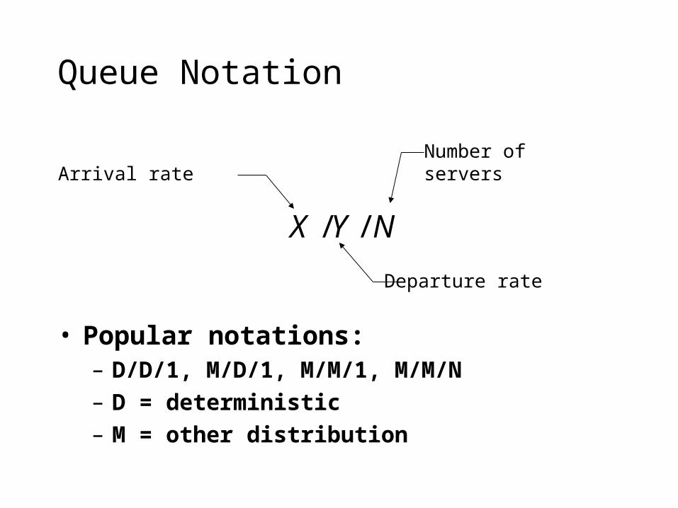
Queue Notation

• Popular notations:– D/D/1, M/D/1, M/M/1, M/M/N– D = deterministic– M = other distribution

NYX //

Arrival rate

Departure rate

Number ofservers

Poisson Distribution

• Good for modeling random events– Standard deviation equals the mean

• Count distribution– Uses discrete values

!n

etnP

tn

P(n) = probability of exactly n vehicles arriving over time t

n = number of vehicles arriving over time t

λ = average arrival rate

t = duration of time over which vehicles are counted

Example Graph

0.00

0.05

0.10

0.15

0.20

0.25

0 1 2 3 4 5 6 7 8 9 10 11 12 13 14 15 16 17 18 19 20

Arrivals in 15 minutes

Pro

bab

ilit

y o

f O

ccu

ran

ce

0.00

0.05

0.10

0.15

0.20

0.25

0 1 2 3 4 5 6 7 8 9 10 11 12 13 14 15 16 17 18 19 20

Arrivals in 15 minutes

Pro

bab

ilit

y o

f O

ccu

ran

ce

Mean = 0.2 vehicles/minute


Example Graph

• If we assume Poisson arrival process• Inter-arrival times are exponentially

distributed

Example: Arrival Intervals

0.0

0.1

0.2

0.3

0.4

0.5

0.6

0.7

0.8

0.9

1.0

0 2 4 6 8 10 12 14 16 18 20

Time Between Arrivals (minutes)

Pro

bab

ilit

y o

f E

xced

ance



Little’s Formula (1961)

• T = time spent by a customer in the queueing system = arrival rate• N = number of customers in the system

• The long-term average number of customers in a stable system N, is equal to the long-term average arrival rate, λ, multiplied by the long-term average time a customer spends in the system, T

• Steady state assumption

)()( EE

Steady State Analysis

• M/D/1– Average length of queue

– Average time waiting in queue

– Average time spent in system

0.1

12

2

Q

12

1w

1

2

2

1t

λ = arrival rate μ = departure rate =traffic intensity

Queue Analysis

• M/M/1– Average length of queue



0.1

1

2

Q

1

w

1t


Queue Analysis

• D/D/1– Average length of queue


– Average time spent in the system

Queue Analysis

• M/M/N– Average length of queue



2

10

1

1

! NNN

PQ

N

1

Q

w

Q

t

0.1N


M/M/N

– Probability of having no vehicles

– Probability of having n vehicles

– Probability of being in a queue

1

0

0

1!!

1N

n

N

c

n

c

c

NNn

P

Nnfor !

0 n

PP

n

n

Nnfor !

0 NN

PP

Nn

n

n

NNN

PP

N

Nn

1!

10

0.1N


Queue times depend on variability

time

items

Can’t store extra capacity

• No reservoir for storing capacity• If capacity goes unused, it is wasted

Queue times depend on variability

Delay will be very different depending on the arrival PATTERN, not just number of arrivals

limitations

• There are many cases when we want to consider changes to the arrival rate

• This is difficult to do when you are limited to steady state assumptions

• Limited number of distributions that provide a closed form expression

Simulation

• In general we are interested in the variability in arrival rates or service times

• If these are constantly varying a steady state assumption is fine

• The alternative is to use a discrete event simulation framework and keep track of individual customers – Microsimulation of an intersection– Queue simulation

Queue simulation

• Simulation based approach• Track vehicles• Step through time• Can change arrival rates, service times,

with knowledge of previous system state• Border wizard

Examples

• Marine terminal• Rail infrastructure• International border• Airport terminal

Port gate and terminal stacks

Gate

Stacks

Observed data

Theoretical wait times

Single server, deterministic service times

0

0.01

0.02

0.03

0.04

0.05

0.06

0.07

0.08

0.09

0.1

10 15 20 25 30 35 40 45 50 55 60 65 70 75 80

Arrival rate

Wai

t ti

me

Rail line as serverAverage Annual Delay (container hours per through container)

-

2.00

4.00

6.00

8.00

10.00

12.00

14.00

16.00

18.00

1,000,000 2,000,000 4,000,000

TEU throughput

Cont

aine

r hou

rs d

elay

per

cont

aine

r thr

ough 7 days a week operation

5 days a week operation

Bottleneck activation

Airport of the Future

• Separates queue intotwo different processes– Check in– Bag check

• Allows travelers to enter mid-stream

Change in terminal processing

K K KK K K KK K KK K

B BB B B B

Baggage flow behind the counter

Queue approaching the counter

P

K K K K KKKK

B

B

B

B

B

B

B

P

Baggage flow

B

Previous system

K

K

K

B

B

B

Airport of the future

K

K

K

B

B

B

Service times got worse!

Total Service Time 2008 2005Mean 07:21 04:59Median 06:35 04:09Standard Deviation 04:46 03:19Sample Variance 00:01 00:00Kurtosis 18:16 07:09Skewness 12:04 58:31Range 31:03 19:45Minimum 00:01 00:38Maximum 31:04 20:23Count 510 352Confidence Level(95.0%)-max 07:46 05:20Confidence Level(95.0%)-min 06:56 04:38

Does not include wait time, only measured from arrival at check-in desk

Total times do improve with AF

• Encourages travelers to check-in online• Reduces perceived wait time

– Start process sooner– Can’t see a big queue

• Reduces employee requirements• Improves space utilization

Border as server

Observations from one day

Regression equations by DOW

Regression equations by Season

Number of very long delays

Proportion of very long delays

Transportation Realities

• For many systems other factors influence delay

• Queing can be used to model wait times• Appropriate tool can be identified on a

case by case basis• Be sure you understand the theoretical

and practical framework

queuing and transportation transportation logistics prof. goodchild spring 2009

Documents