quasi-steady analytical model benchmark of an impulse

Hindawi Publishing CorporationInternational Journal of Rotating MachineryVolume 2008, Article ID 536079, 12 pagesdoi:10.1155/2008/536079

Research ArticleQuasi-Steady Analytical Model Benchmark ofan Impulse Turbine for Wave Energy Extraction

A. Thakker, J. Jarvis, and A. Sahed

Department of Mechanical & Aeronautical Engineering, Materials and Surface Science Institute,University of Limerick, Limerick, Ireland

Correspondence should be addressed to A. Sahed, [email protected]

Received 15 April 2008; Accepted 11 September 2008

Recommended by Ion Paraschivoiu

This work presents a mean line analysis for the prediction of the performance and aerodynamic loss of axial flow impulse turbinewave energy extraction, which can be easily incorporated into the turbine design program. The model is based on the momentumprinciple and the well-known Euler turbine equation. Predictions of torque, pressure drop, and turbine efficiency showed favorableagreement with experimental results. The variation of the flow incidence and exit angles with the flow coefficient has been reportedfor the first time in the field of wave energy extraction. Furthermore, an optimum range of upstream guide vanes setting up anglewas determined, which optimized the impulse turbine performance prediction under movable guide vanes working condition.

Copyright © 2008 A. Thakker et al. This is an open access article distributed under the Creative Commons Attribution License,which permits unrestricted use, distribution, and reproduction in any medium, provided the original work is properly cited.

1. INTRODUCTION

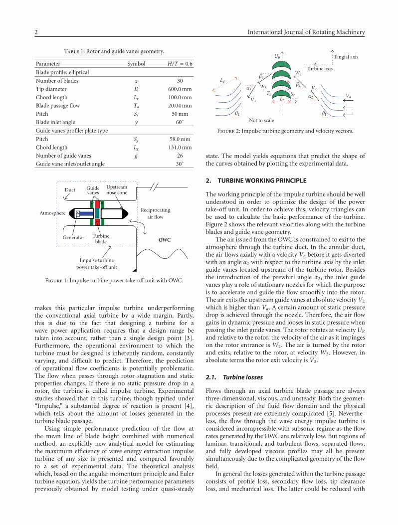
The oscillating water column (OWC) wave energy harnessingmethod is considered as one of the best techniques ofconverting wave energy into electricity. It is an economicallyviable design due to its simple geometrical construction, andis also strong enough to withstand against the waves withdifferent heights, periods, and directions. The design (seeFigure 1) consists of an OWC chamber and a circular duct,which reciprocally moves the air from and into the chamberas the wave enters and intercedes from the chamber. Thewave energy is converted into air pneumatic energy inside thechamber. A special turbine mounted inside the duct convertsthe air pneumatic energy to a mechanical power. A matchinggenerator is coupled to the turbine to produce electricity [1].

In order to use the potential wave energy resource,efficiently, turbine design/operation with low losses, highefficiency, and desirable performance is needed. The effi-ciency is a measure of performance and a poorly performingturbine becomes unavailable for power plant. Therefore asound knowledge of the turbine efficiency limits is necessaryfor the power take-off design/operation.

The impulse turbine discussed here is one of a class ofturbines called self-rectifying turbines, that is, turbines thatrotate in the same direction no matter what the direction

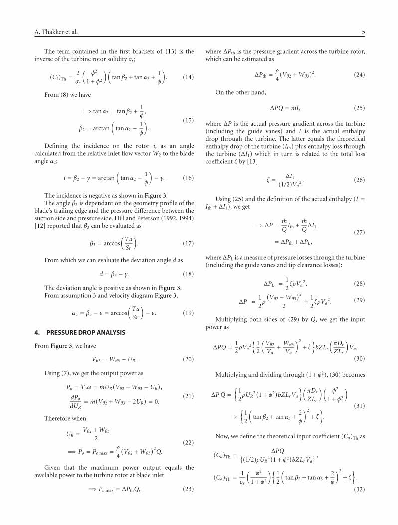
of the airflow is. Self-rectifying turbines are a response tothe need for turbines to extract power from bidirectionalairflows that arise in wave power applications such as theOWC. The basic turbine design parameters were based on theoptimum design parameters given by Setoguchi and Takao[2], but with a H/T ratio of 0.6. The details are given inTable 1 and a 2D sketch at mid radius is shown in Figure 2.The rotor consists of 30 blades with a chord length, Lr =100 mm and pitch, Sr = 50 mm. There are 26 fixed anglemirror image guide vanes on both sides of the rotor. Theguide vanes inlet/outlet angle is fixed at 30◦. The turbinewas tested at a constant axial air velocity of 7.22 m/s. Datawere collected with the help of data acquisition system tominimize the errors. Experiments were performed by varyingthe rotational speed from 1300 to 100 rpm, thus giving a flowcoefficient range of 0.22–2.90 under unidirectional steadyflow conditions. The peak efficiency of 44.6% was achievedat φ = 0.88, corresponding to a rotational speed of 300 rpm.The Reynolds number at the peak efficiency point was 0.92×105.

The state-of-the-art of the wave energy impulse turbineis crucially getting closer to an actual prototype and ananalytical model of the turbine derived from first principleswould prove necessary. Thus far, the highest efficiencyreported by model testing has been 50% at most, which

2 International Journal of Rotating Machinery

Table 1: Rotor and guide vanes geometry.

Parameter Symbol H/T = 0.6

Blade profile: elliptical

Number of blades z 30

Tip diameter D 600.0 mm

Chord length Lr 100.0 mm

Blade passage flow Ta 20.04 mm

Pitch Sr 50 mm

Blade inlet angle γ 60◦

Guide vanes profile: plate type

Pitch Sg 58.0 mm

Chord length Lg 131.0 mm

Number of guide vanes g 26

Guide vane inlet/outlet angle 30◦

Duct Guidevanes

Upstreamnose cone

Atmosphere

Generator OWCTurbine

blade

Impulse turbinepower take-off unit

Reciprocatingair flow

Figure 1: Impulse turbine power take-off unit with OWC.

makes this particular impulse turbine underperformingthe conventional axial turbine by a wide margin. Partly,this is due to the fact that designing a turbine for awave power application requires that a design range betaken into account, rather than a single design point [3].Furthermore, the operational environment to which theturbine must be designed is inherently random, constantlyvarying, and difficult to predict. Therefore, the predictionof operational flow coefficients is potentially problematic.The flow when passes through rotor stagnation and staticproperties changes. If there is no static pressure drop in arotor, the turbine is called impulse turbine. Experimentalstudies showed that in this turbine, though typified under“Impulse,” a substantial degree of reaction is present [4],which tells about the amount of losses generated in theturbine blade passage.

Using simple performance prediction of the flow atthe mean line of blade height combined with numericalmethod, an explicitly new analytical model for estimatingthe maximum efficiency of wave energy extraction impulseturbine of any size is presented and compared favorablyto a set of experimental data. The theoretical analysiswhich, based on the angular momentum principle and Eulerturbine equation, yields the turbine performance parameterspreviously obtained by model testing under quasi-steady

Lg

θ2

Lr

α3

V3

β3

W3

Ta Srγ

UR

β2

W2

V2

α2

θ1

Va

Tangial axis

Turbine axis

Not to scale

Figure 2: Impulse turbine geometry and velocity vectors.

state. The model yields equations that predict the shape ofthe curves obtained by plotting the experimental data.

2. TURBINE WORKING PRINCIPLE

The working principle of the impulse turbine should be wellunderstood in order to optimize the design of the powertake-off unit. In order to achieve this, velocity triangles canbe used to calculate the basic performance of the turbine.Figure 2 shows the relevant velocities along with the turbineblades and guide vane geometry.

The air issued from the OWC is constrained to exit to theatmosphere through the turbine duct. In the annular duct,the air flows axially with a velocity Va before it gets divertedwith an angle α2 with respect to the turbine axis by the inletguide vanes located upstream of the turbine rotor. Besidesthe introduction of the prewhirl angle α2, the inlet guidevanes play a role of stationary nozzles for which the purposeis to accelerate and guide the flow smoothly into the rotor.The air exits the upstream guide vanes at absolute velocity V2

which is higher than Va. A certain amount of static pressuredrop is achieved through the nozzle. Therefore, the air flowgains in dynamic pressure and looses in static pressure whenpassing the inlet guide vanes. The rotor rotates at velocity UR

and relative to the rotor, the velocity of the air as it impingeson the rotor entrance is W2. The air is turned by the rotorand exits, relative to the rotor, at velocity W3. However, inabsolute terms the rotor exit velocity is V3.

2.1. Turbine losses

Flows through an axial turbine blade passage are alwaysthree-dimensional, viscous, and unsteady. Both the geomet-ric description of the fluid flow domain and the physicalprocesses present are extremely complicated [5]. Neverthe-less, the flow through the wave energy impulse turbine isconsidered incompressible with subsonic regime as the flowrates generated by the OWC are relatively low. But regions oflaminar, transitional, and turbulent flows, separated flows,and fully developed viscous profiles may all be presentsimultaneously due to the complicated geometry of the flowfield.

In general the losses generated within the turbine passageconsists of profile loss, secondary flow loss, tip clearanceloss, and mechanical loss. The latter could be reduced with

A. Thakker et al. 3

improved manufacturing and assembling technology, andprofile and secondary flow loss (60%) could be reducedby designing a turbine to operate at optimum designparameters. However, there are many design parameters forminimizing aerodynamic losses within the turbine passage.Among them, the incidence angle is the most importantas it is immediately related to the aerodynamic losses [6].The guide vanes and blade profile losses can be significantif the blade shapes are not optimized for the local operatingconditions. Profile losses are driven by surface finish, totalblade surface area, blade shape and surface velocity distribu-tions, and proper matching between guide vane and bladeto minimize incidence losses. Equally significant losses canbe caused by the complex secondary flows generated as theviscous boundary layers along the pressure and suction of theair path are turned through the blade passage.

The clearance between the blade tips and casing end-wall in a turbine induces leakage flow, which arises due topressure difference between the pressure surface and suctionsurface of the blade. The leakage flow emerging from theclearance interacts with the passage flow (main stream) androlls up into a vortex known as tip leakage vortex. Althoughthe size of the clearance is typically about 1% of the bladeheight, the leakage flow through this small clearance has asignificant effect on the aerodynamics of the turbine. Forexample, the tip clearance loss of a turbine blade can accountfor as much as one-third of the total losses [7]. The tipleakage loss is driven by the higher reaction levels at the bladetip, which increases the pressure drop across the blade tip.

In contrast to the general design problem familiar inindustry (e.g., steam and gas turbines), where a turbinewould be expected to operate at a single design point for themajority of the time, the performance of a turbine intendedfor use in a wave energy application must be consideredover a range of flow coefficient. This is a consequence ofthe constantly changing and bidirectional nature of theairflow (varying loads), thus designing a turbine to a wavepower application requires that a design range be taken intoaccount, rather than a single design point [3]. Nevertheless,a certain similarity can be found between the steam impulseturbine and the self-rectifying impulse turbine as for both thefluid’s pressure is changed to velocity by accelerating the fluidwith a nozzle and upstream guide vane, respectively. Also, thesteam rotor blade can be recognized by its shape, which issymmetrical about the rotor midchord and has inlet and exitangles around 20◦. It has constant cross section from hub totip, which is almost similar to that of the wave energy impulseturbine.

2.2. Flow incidence and deviation angle

The relative inlet flow vector at blade leading edge (W2) isnot a simple geometric value but a measured parameter;that is, it depends on the rotational speed and the absoluteflow velocity. The incidence i on the rotor is defined as anangle calculated from the relative inlet flow vector to theblade inlet angle (see Figure 3). Optimizing the incidencewould minimize pressure losses in the blade passage, whichthe turbine efficiency is directly related to. The optimum

Velocity+

Angle+

γ

α3

V3 ε

dW3

β3

Vθ3

UR

Wθ3

Va

α2

W2

V2

−iβ2

Va

ε

UR

Wθ2

Vθ2

Tangial axis

Turbine axis

Figure 3: Velocity triangles.

incidence depends on the input power as well as the bladeprofile. The range of applicable incidence becomes narrowwhen the turbine operates at high input power [8]. Also,due to Cho and Choi [8] the optimum is for small negativevalues (around −20◦) but the efficiency quickly drops asthe incidence grows to negative over the range of applicableincidence, in which case the flow tends to strike the bladeleading edge axially and beyond.

The angle of the flow leaving the blade at the trailingedge (β3) is of great importance as it determines themagnitude of relative exit flow at blade trailing edge (W3).The deviation angle (d) from the rotor is defined as an anglecalculated from the relative exit flow vector to the bladeexit angle. Assuming that the axial velocity and the relativetangential velocity remain the same (for optimum designflow coefficient), the angle β3 is dependant on the geometryprofile of the blade’s trailing edge and the pressure differencebetween the suction side and pressure side [4, 9].

The basic objective of the turbine design is that the bladeangles at inlet and exit γ must be matched properly withthe fluid flow angles (β2, β3), respectively. They need notnecessarily be equal, but should be matched properly tominimize losses [4].

The absolute angle (α3) at the blade trailing edge isequally important as it determines the absolute velocity (V3)by which the air flow enters the inlet of the downstreamguide vanes. If the angle α3 is close to 60◦, the metal bladeangle, then the air would enter the downstream guide vanesswiftly as the air flow direction would be parallel to thestraight portion of the guide vanes. Under this condition,the wave energy impulse turbine would be working atmaximum efficiency because of the reduced losses throughthe downstream guide vanes [4, 9]. These losses are known,from experimental work, to be substantial and directly affectthe turbine efficiency. Outside the above working condition,the air will strike the guide vanes more or less axially, causingbigger losses. In the latter case, the turbine is said to beoff-designed. For an ideal wave energy impulse turbine, α3

should also match the setting up angle of the downstream


guide vanes, θ2, which adds to the complexity of the design(see Figure 2).

2.3. Turbine performance evaluation

Thus far the turbine characteristics under steady flowconditions have been obtained by model testing and wereevaluated according to the torque coefficient Ct , input powercoefficient Ca and flow coefficient φ, which are defined bySetoguchi and Takao [2]:

Ct = To(1/2)ρa

(Va

2 +UR2)bZLrrR

, (1)

Ca = ΔPQ

(1/2)ρa(Va

2 +UR2)bZLrVa

, (2)

φ = Va

UR, (3)

Re =ρa√Va

2 +UR2Lr

μ, (4)

η = CtCa φ

, (5)

where Re is the Reynolds number based on the chord length,To: measured output torque, ρa: density of air, b: rotorblade height, UR: circumferential at rR, Va: mean axial flowvelocity, rR: mean radius, Z number of rotor blades, ΔP:measured total pressure drop between settling chamber andatmosphere, and Q: flow rate. The test Reynolds numberbased on the chord was 0.4× 104.

On the other hand, it was reported in [10] that the quasi-steady torque and input coefficient were higher, especiallyat high flow coefficient than those found when the turbineis operated under unsteady flow conditions. Also, the drop-off in efficiency under steady state at high flow coefficientwas not seen under sinusoidal flow pattern. Furthermore, thesinusoidal testing showed that if the efficiency is consideredthrough the complete sinusoidal wave, it is relatively con-stant. Therein, it is therefore important that future turbinesare designed with this in mind due to the difference betweenthe results found from unsteady testing and those predictedusing fixed flow testing.

Velocity triangles can be constructed at any sectionthrough the blades (e.g., hub, tip, midsection, etc.) usingthe various velocity vectors, but are usually shown at themean radius. The obvious snag is that of the reduction inaerodynamic design work. At other radii velocity triangleswill vary, demanding the introduction of either blade orguide vanes twisting [11]. Nevertheless, it is known that theefficiency of a properly designed axial flow turbine can bepredicted with fair accuracy (1 or 2%) by the adoption ofsimple mean line analysis methods which incorporate properloss and flow angle correlations [12].

Similar to simple theory for ordinary turbo-machine, thefollowing assumption can be given to analyze the turbineperformance.

(i) Turbine performance is estimated from condition atmean radius.

(ii) Absolute nozzle exit flow angle α2, the complementof θ1, is constant.

(iii) Relative rotor exit flow angle is constant, β3.

Due to blade symmetry of this particular design ofself rectifying turbine we can state that

(iv) the angles between the relative flow vector and theabsolute velocity vector at inlet and outlet of the rotorare identical (ε).

3. TORQUE ANALYSIS

Applying “momentum principle—Newton’s second law,” thetorque generated by the turbine shaft due to the tangentialmomentum change of air passing through the turbine rotorcan be evaluated as follows [11]:

Generated torque = rate of change of moment of

momentum:

To = d

dt

(mrRΔV

). (6)

Replacing the expression of change of air whirl velocityin (6), we get

To = mrRUR

(Vθ2

UR+Vθ3

UR

). (7)

From the velocity diagram of Figure 3, we have

Vθ2

UR= φ

(Wθ2 +UR

Va

)= φ tanβ2 + 1,

Vθ3

UR= φ tanα3.

(8)

Replacing (8) in (7), the torque is expressed as

To = mrRURφ(

tanβ2 + tanα3 +1φ

). (9)

By the replacement for the expression of m and usingblade height, chord length, and flow coefficient definition,we get from (9)

To = 12ρUR

2bZLrrR2(πDr

ZLr

)φ2(

tanβ2 + tanα3 +1φ

).

(10)

Multiplying and dividing (10) through (1 + φ2), we get

To ={

12ρUR

2(1 + φ2)bZLrrR

}2(πDr

ZLr

)(φ2

1 + φ2

)

×(

tanβ2 tanα3 +1φ

).

(11)

Now, we define the theoretical torque coefficient (Ct)Th

as

(Ct)Th =To{

(1/2)ρUR2(1 + φ2

)bZLrrR

} , (12)

(Ct)Th = 2(πDr

ZLr

)(φ2

1 + φ2

)(tanβ2 + tanα3 +

1φ

). (13)

A. Thakker et al. 5

The term contained in the first brackets of (13) is theinverse of the turbine rotor solidity σr ;

(Ct)Th =2σr

(φ2

1 + φ2

)(tanβ2 + tanα3 +

1φ

). (14)

From (8) we have

=⇒ tanα2 = tanβ2 +1φ

,

β2 = arctan(

tanα2 − 1φ

).

(15)

Defining the incidence on the rotor i, as an anglecalculated from the relative inlet flow vector W2 to the bladeangle α2;

i = β2 − γ = arctan(

tanα2 − 1φ

)− γ. (16)

The incidence is negative as shown in Figure 3.The angle β3 is dependant on the geometry profile of the

blade’s trailing edge and the pressure difference between thesuction side and pressure side. Hill and Peterson (1992, 1994)[12] reported that β3 can be evaluated as

β3 = arccos(Ta

Sr

). (17)

From which we can evaluate the deviation angle d as

d = β3 − γ. (18)

The deviation angle is positive as shown in Figure 3.From assumption 3 and velocity diagram Figure 3,

α3 = β3 − ε = arccos(Ta

Sr

)− ε. (19)

4. PRESSURE DROP ANALYSIS

From Figure 3, we have

Vθ3 =Wθ3 −UR. (20)

Using (7), we get the output power as

Po = Toω = mUR(Vθ2 +Wθ3 −UR

),

dPodUR

= m(Vθ2 +Wθ3 − 2UR

) = 0.(21)

Therefore when

UR = Vθ2 +Wθ3

2

=⇒ Po = Po,max =ρ

4

(Vθ2 +Wθ3

)2Q.

(22)

Given that the maximum power output equals theavailable power to the turbine rotor at blade inlet

=⇒ Po,max = ΔPthQ, (23)

where ΔPth is the pressure gradient across the turbine rotor,which can be estimated as

ΔPth =ρ

4(Vθ2 +Wθ3)2. (24)

On the other hand,

ΔPQ = mI , (25)

where ΔP is the actual pressure gradient across the turbine(including the guide vanes) and I is the actual enthalpydrop through the turbine. The latter equals the theoreticalenthalpy drop of the turbine (Ith) plus enthalpy loss throughthe turbine (ΔI1) which in turn is related to the total losscoefficient ζ by [13]

ζ = ΔI1(1/2)Va

2 . (26)

Using (25) and the definition of the actual enthalpy (I =Ith + ΔI1), we get

=⇒ ΔP = m

QIth +

m

QΔI1

= ΔPth + ΔPL,

(27)

whereΔPL is a measure of pressure losses through the turbine(including the guide vanes and tip clearance losses):

ΔPL = 12ζρVa

2, (28)

ΔP = 12ρ

(Vθ2 +Wθ3

)2

2+

12ζρVa

2. (29)

Multiplying both sides of (29) by Q, we get the inputpower as

ΔPQ = 12ρVa

2{

12

(Vθ2

Va+Wθ3

Va

)2

+ ζ}bZLr

(πDr

ZLr

)Va.

(30)

Multiplying and dividing through (1 +φ2), (30) becomes

ΔP Q ={

12ρUR

2(1 + φ2)bZLrVa

}(πDr

ZLr

)(φ2

1 + φ2

)

×{

12

(tanβ2 + tanα3 +

2φ

)2

+ ζ}.

(31)

Now, we define the theoretical input coefficient (Ca)Th as

(Ca)Th =ΔPQ

{(1/2)ρUR

2(1 + φ2)bZLrVa

} ,

(Ca)Th =1σr

(φ2

1 + φ2

){12

(tanβ2 + tanα3 +

2φ

)2

+ ζ}.

(32)


4.1. Loss coefficient ζ

Losses in turbines are used to be expressed in terms of losscoefficients. They are manifested by a decrease in stagnationenthalpy, and a variation in static pressure, compared to theisentropic flow. The commonly used loss coefficient is thestagnation pressure loss coefficient, which is convenient forexperimental work and especially for this particular impulseturbine. Wei [14] has reported in his doctoral thesis byreferring back to Horlock [15] that the incidence is the mostimportant parameter to predict the off-design profile loss.The stagnation pressure loss coefficient in the relative frameis defined as [16]

ζR = P02,rel − P03,rel

(1/2)ρW22 , (33)

where P0,rel = P + (1/2)ρW2 is the relative total pressure atblade inlet and outlet (2, 3), respectively.

From (33) we have

ζR =(P2 + (1/2)ρW2

2)− (P3 + (1/2)ρW32)

(1/2)ρW22 , (34)

ζR =(P2 + (1/2)ρW2

2)− (P3 + (1/2)ρW32)

(1/2)ρW22

+(1/2)ρ

(V2

2 −V22) + (1/2)ρ

(V3

2 −V32)

(1/2)ρW22 ,

(35)

ζR =(P2 + (1/2)ρV2

2)− (P3 + (1/2)ρV32)

(1/2)ρW22

+

(W2

2 −V22) +

(V3

2 −W32)

W22 .

(36)

Multiplying and dividing through V22 (36), rearranging

we get

ζR =(V2

W2

)2

⎧⎪⎪⎪⎪⎨

⎪⎪⎪⎪⎩

(P2 + (1/2)ρV2

2)− (P3 + (1/2)ρV32)

(1/2)ρV22

︸︷︷︸A

+(W2

V2

)2

− 1 +(V3

V2

)2

−(W3

V2

)2

︸︷︷︸B

⎫⎪⎪⎪⎪⎬

⎪⎪⎪⎪⎭

.

(37)

Applying Euler turbine equation [10],(P2 +

12ρV2

2)−(P3 +

12ρV3

2)= ρUR

(Vθ2 +Vθ3

)(38)

=⇒ A = ρUR(Vθ2 +Vθ3

)

(1/2)ρV22 (39)

A = 2(UR

V2

)2(Va

UR

)(Vθ2

Va+Vθ3

Va

). (40)

From Figure 3 we haveV2 = Va/ cosα2, tanα2 = Vθ2/Va,and tanα3 = Vθ3/Va

=⇒ A = 2φ

(cosα2

)2(tanα2 + tanα3

). (41)

Also, from Figure 3 we have W2 = Va/ cosβ2, W3 =Va/ cosβ3, and V3 = Va/ cosα3

=⇒ B = ( cosα2)2{

1(

cosβ2)2 −

1(

cosα2)2

+1

(cosα3

)2 −1

(cosβ3

)2

}

.

(42)

By replacing (39) and (42) in (37), simplifying, andrearranging, we get

ζR =(

cosβ2)2{

2(

tanα2 + tanα3)

φ+

1(

cosβ2)2

− 1(

cosα2)2 +

1(

cosα3)2 −

1(

cosβ3)2

}

,

(43)

ζR accounts only for aerodynamic losses (profile and sec-ondary flow losses, which cannot be separated) through theblade passage. These are greatly affected by the flow incidence[7, 11]. Therefore the tip clearance loss and the loss in theturbine stationary guide vanes are not accounted for. Forthis, an underestimation of the actual losses is to be expectedwhen only using the losses in the rotor (43). The actuallosses would be accurately simulated if we could have anexpression of ζ which accounts for all the losses in the turbine(including tip clearance leakage, guide vanes, near hub, andcasing walls losses). For the particular WERT test rig, UL, thedata logger acquisition compensates the torque measurementfor the mechanical and windage losses.

It was reported from model testing that substantialstagnation pressure drop across the downstream guide vaneexists causing losses. To take these into account, estima-tion from three-dimensional computational fluid dynamics(CFD) of the losses across the downstream guide vanes wasutilized.

The variation of pressure loss coefficient through thedownstream guide vane at various stations from hub to tipwas computed for the flow coefficients φ = 0.45, 0.67, 1, 1.35,and 1.68, respectively. The total pressure loss coefficient hasbeen defined as follows [17–19]:

ζGV = Poi − PoPoi − Psi

, (44)

where P is the pressure and the subscripts i, o, and s denoteinlet conditions, total and static conditions, respectively.

Then, the arithmetic mean of the computed values fromhub to tip for each flow coefficient were calculated, plottedand an optimum curve fit correlation (ζGV = f (φ)) wasestablished as illustrated in Figure 4;

ζGV = 5.78φ

− 1.85. (45)

The correlation of the downstream guide vane loss (45)derived from validated computational (CFD) work should be

A. Thakker et al. 7Lo

ssco

effici

ent

dow

nst

ream

guid

eva

ne

(ζD

GV

)

5

10

15

20

25

Flow coefficient (φ)

0 0.5 1 1.5 2 2.5 3 3.5

CorrelationAverage computational

ζGV = 5.78/φ − 1.85

Figure 4: Correlated downstream guide vane loss coefficient versusflow coefficient [10].

Torq

ue

coeffi

cien

t(C

t)

0

0.5

1

1.5

2

2.5

3

3.5


0 0.5 1 1.5 2 2.5 3 3.5

(Ct)experimental

(Ct)theoretical

Figure 5: Turbine torque coefficient versus flow coefficient [10].

considered specific for the design of impulse turbine waveenergy extraction;

ζ = ζR + ζGV. (46)

5. RESULTS AND DISCUSSION

Figure 5 shows the theoretical and experimental torquecoefficient versus flow coefficient. The torque coefficientfollows an exponential trend up to flow coefficient (φ =0.8) then a short transition occurs and the trend becomeslogarithmic in nature for the rest of the flow coefficient.There is no apparent stall, as opposed to the Wells turbine. Itcan be seen that the model’s torque coefficient predicts wellthe shape of the torque coefficient obtained by plotting theexperimental data. The prediction seems to be almost perfectat low flow coefficient (up to φ = 0.8) and then a smalldiscrepancy appears for the rest of the flow coefficient.

Flow

inci

den

cean

dab

solu

teex

itan

gle

(i,α◦ 3)

−120

−100

−80

−60

−40

−20

0

20

40

60

80


0 0.5 1 1.5 2 2.5 3 3.5

iα3

Figure 6: Flow incidence and absolute exit angle versus flowcoefficient.

Figure 6 shows the variation of the incidence angle (i)and absolute exit angle (α3), calculated from (16) and (19),respectively, with the flow coefficient. The incidence angle,directly related to the profile geometry [9], is very high(negative) at low flow coefficients (high rotational speed)making the air flow relatively impinging at the suction sideof the leading edge. In other word, the stagnation point islocated at the suction side of the leading edge and the airflow acts as a break on the turbine. This would be the mainreason of the negative torque obtained experimentally [4]. Asthe flow coefficient increases a rapid decline of the incidenceoccurs from −120◦ at φ = 0.29 up to φ = 1.1 at which itreaches −20◦, where the turbine efficiency reaches a plateau.The optimum incidence angle for wave energy impulseturbine is for small negative values (around −20◦) similarto that reported in [5]. At this condition the stagnationpoint is located close on the end profile camber line. As theflow coefficient continues increasing the incidence angle isdecreasing almost steadily to reach a value of −4.5◦ at thehighest flow coefficient of φ = 3.57. At this low incidenceangle the relative flow angle (β2, (16)) is almost alignedwith the blade angle (γ) presenting a supposedly optimumworking conditions, where the incidence angle ensures thesmoothest entry condition into the turbine rotor blade.

The trend of the exit angle is similar, but varies in phase(66◦) with the incidence angle, Figure 6. At very low flowcoefficient φ = 0.29, the absolute exit flow angle is about−55◦ causing the flow to impinge onto the downstream guidevane straight portion vertically (the ideal is when the flowdirection is parallel to the downstream guide vane straightportion, smooth entry). Then, a rapid decrease (from highnegative value) of the exit flow angle is shown with theincrease of flow coefficient, reaching 46◦ at φ = 1.1. Atthis flow coefficient the flow entering the inlet guide vane isrelatively smooth. In between the above two flow coefficients,there was a condition where the exit flow vector V3 becamealigned with the axial flow vector Va, precisely at a value offlow coefficient φ = 0.53. As the flow coefficient continues


Inpu

tco

effici

ent

(Ca)

0.5

1

1.5

2

2.5

3

3.5

4

4.5


0 0.5 1 1.5 2 2.5 3 3.5 4

(Ca)experimental

(Ca)theoretical

Figure 7: Turbine input coefficient versus flow coefficient [10].

beyond φ = 1.1, a steady increase of exit flow angle is shownup to the highest flow coefficient of φ = 3.57 at which itreaches 62.8◦. During the steady increase of the absolute exitflow angle, a favorable working condition sets up, where theexit flow vector becomes closer to the alignment with thedownstream guide vane. This will reduce greatly the lossesthrough downstream guide vanes as will be shown below.

Figure 7 displays the input coefficient theoretical andexperimental data versus flow coefficient in the case ofthe losses through the rotor passage and the downstreamguide vanes were taken into account (based on experimentalanalysis the upstream guide vane losses were found to be low[4, 9]). It can be seen that the discrepancy is smaller relativeto the earlier case especially at low flow coefficient. Also theslope of the model input coefficient at high flow coefficientis almost zero (no change). Whereas at high flow coefficient,the experimental input coefficient seems to increase with theflow coefficient. This could be explained by the boundarylayer separation losses at the blade suction side caused bythe high inlet relative flow angle (low incidence angle) andhigher loading. Also the contention for the front part ofthe blade tip could be blocked by the inlet boundary layer“aerodynamically closed” and therefore could be sustainingthe horseshoe vortex system [18]. Moreover the tip leakagevortex, which is not incorporated in the model, increasesseparation. Previous author’s results [19] obtained from CFDand validated experimentally showed up to 4% of lossescould be generated by the gap existing between the blade tipand the duct inner surface for the specific impulse turbinewave energy extraction.

Figure 8 shows the turbine efficiency from the experi-mental as well as theoretical data, which is typical of theimpulse turbine used for wave energy conversion [2]. At lowlevels of flow coefficient it can be seen that the efficiency isvery sensitive to changes in the flow coefficient. Furthermore,the experimental efficiency was maximum (η = 44.6%)at flow coefficient (φ = 0.88) which is known as theoptimum flow coefficient and the Reynolds number was(Re = 0.92 × 105). Subsequently, the efficiency decreases

Effi

cien

cy(η

)

0.1

0.15

0.2

0.25

0.3

0.35

0.4

0.45

0.5


0 0.5 1 1.5 2 2.5 3 3.5 4

ηexperimental

ηtheoretical

Figure 8: Turbine efficiency versus flow coefficient [10].

as the flow coefficient is further increased, although itssensitivity to changes in flow coefficient diminishes. Low flowcoefficient thus greatly reduces the efficiency to an extent thatthe high flow coefficient does not. This is due to the incidenceangle which is very high (negative) at low flow coefficients,making the air flow relatively impinging at the suctionside of the leading edge. This is shown experimentallyas a small positive value or even negative torque in theregion of very low coefficient. Also the low flow coefficientregion is characterized with instable working conditionswhere the efficiency could drop or rise sharply for a smallturbine angular velocity increase or decrease, respectively.Nevertheless, as the flow coefficient starts increasing fromminimum the turbine picks up in performance sharply toreach the optimum. The reason is that the boundary layersare of type turbulent, due to higher Reynolds number inwhich case the flow separation does not exist. Also at lowflow coefficient the turbine inertia is high helping the turbineto reach the optimum performance quickly. The conjugationof these two effects overcomes the very high flow incidenceangle effect.

At high flow coefficient though the incidence angleis optimum because of the low turbine rotational speed,still we notice a slight drop in the turbine performance.This can be explained by the effect of boundary layers oftype laminar, due to lower Reynolds number, which areprone to separation especially in the tip region [14]. In theboundary layer regions, the velocity deficit and the totalpressure loss increase as the Reynolds number decreases(high flow coefficient). Also, here the inertia is not helpingto recover the turbine performance as it is low becauseof the low rotational speed. At moderate flow coefficientthe turbine performance is at maximum and the workingcondition is stable, that is, there is no sudden change inturbine characteristics within this region of flow coefficient.However, the incidence angle and the boundary layersare not favorable in this moderate flow conditions. Thishigh turbine efficiency working region can be character-ized as the compromising region, between the incidence

A. Thakker et al. 9Lo

ssco

effici

ent

(ζ)

−0.6

2

4

6

8

10

12

14

16

18


0.5 1 1.5 2 2.5 3 3.5

{ζGV}experimental

{ζGV}theoretical

{ζR}theoretical

{ζR}experimental

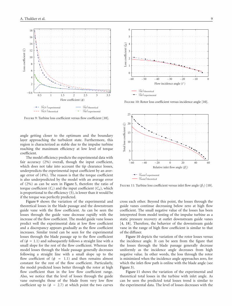
Figure 9: Turbine loss coefficient versus flow coefficient [10].

angle getting closer to the optimum and the boundarylayer approaching the turbulent state. Furthermore, thisregion is characterized as stable due to the impulse turbinereaching the maximum efficiency at low level of torquecoefficient.

The model efficiency predicts the experimental data withfair accuracy (2%) overall, though the input coefficient,which does not take into account the tip clearance losses,underpredicts the experimental input coefficient by an aver-age error of (4%). The reason is that the torque coefficientis also underpredicted by the model with an average errorof (2%) as can be seen in Figure 5, therefore the ratio oftorque coefficient (Ct) and the input coefficient (Ca), whichis proportional to the efficiency (5), is lower than it would beif the torque was perfectly predicted.

Figure 9 shows the variation of the experimental andtheoretical losses in the blade passage and the downstreamguide vane with the flow coefficient. As can be seen thelosses through the guide vane decrease rapidly with theincrease of the flow coefficient. The model guide vane lossespredict well the experimental data at low flow coefficientand a discrepancy appears gradually as the flow coefficientincreases. Similar trend can be seen for the experimentallosses through the blade passage up to the flow coefficientof (φ = 1.1) and subsequently follows a straight line with asmall slope for the rest of the flow coefficient. Whereas themodel losses through the blade passage generally decreasesfollowing a straight line with a small slope up to theflow coefficient of (φ = 1.1) and then remains almostconstant for the rest of the flow coefficient. Particularly,the model predicted loses better through the rotor at highflow coefficient than in the low flow coefficient range.Also, we notice that the level of losses through the guidevane outweighs those of the blade from very low flowcoefficient up to (φ = 2.7) at which point the two curves

Loss

coeffi

cien

t(ζR

)

0

1

2

3

4

5

6

Flow incidence angle (i◦)

−60 −50 −40 −30 −20 −10 0

{ζR}theoretical

{ζR}experimental

Figure 10: Rotor loss coefficient versus incidence angle [10].

Tota

llos

sco

effici

ent

(ζ)

0

5

10

15

20

25

Relative inlet flow angle (β◦2)

−60 −40 −20 0 20 40 60

{ζtotal}experimental

{ζtotal}theoretical

Figure 11: Turbine loss coefficient versus inlet flow angle (β2) [10].

cross each other. Beyond this point, the losses through theguide vanes continue decreasing below zero at high flowcoefficient. The small negative value of the losses has beeninterpreted from model testing of the impulse turbine as astatic pressure recovery at outlet downstream guide vanes[4, 18]. Therefore, the behavior of the downstream guidevane in the range of high flow coefficient is similar to thatof the diffuser.

Figure 10 depicts the variation of the rotor losses versusthe incidence angle. It can be seen from the figure thatthe losses through the blade passage generally decreaseuniformly as the incidence angle decreases from highnegative value. In other words, the loss through the rotoris minimized when the incidence angle approaches zero, forwhich the inlet-flow path is online with the blade angle (seeFigure 3).

Figure 11 shows the variation of the experimental andtheoretical total losses in the turbine with inlet angle. Ascan be seen the predicted total losses trend is similar tothe experimental data. The level of losses decreases with the

10 International Journal of Rotating MachineryTo

tall

oss

coeffi

cien

t(ζ

)

100

101

102

Relative inlet flow angle (β◦2)

−60 −40 −20 0 20 3035 40 50 60

{ζtotal}experimental

{ζtotal}theoretical

Figure 12: Turbine loss coefficient versus inlet flow angle (β2) [10].

increase of relative inlet flow angle following two differentcurvatures with an inflexion point that is located at β2 = 0◦.The latter angle does not represent the minima point as seenfrom Figure 11. The minima scenario would be typical to areaction turbine with an optimum angle not necessarily 0◦

[11]. Therefore, though the reported experimental pressuredrop across the turbine rotor was substantial [4, 18], theloss reported in the present study reinforces the impulsecharacteristic of this particular turbine for which there isno negative or positive stall. In other word, there is no highpositive or negative incidence for which the air flow separatescatastrophically from the blade surface resulting in suddencollapse of torque and increase in pressure drop and thereforeof loss.

In order to identify the optimum inlet flow angle forwhich the impulse turbine efficiency is maximum, a semiloggraph was used.

As we can see from Figure 12, the total loss coefficientfollows a straight portion with a moderate slope from lowinlet angle up to around β2 = 35◦ from which point theloss starts decreasing rapidly for the rest of the turbineoperational range. As a result the optimum inlet flow angle,at which the turbine efficiency is maximum (the optimumperformance of this particular turbine is reached at lowerlevel of flow coefficient), was found to be β2 = 35◦. Theexperimental value reported in [4] was β2 = 33.8◦.

Figure 13 shows variation of the optimum upstreamguide vane angle with the flow coefficient while keepingthe relative inlet flow angle optimum β2 = 35◦. For lowerflow coefficient, the guide vane angle is small because of thelower input power, whereas at higher flow coefficient region,where the impulse turbine is known to handle larger inputpower without drastic decrease of efficiency (unlike the Wellsturbine), the guide vane angle is larger. This is in order tosatisfy the turbine optimum relative inlet angle.

Figure 14 shows the model prediction of the impulseturbine efficiency when the upstream guide vanes settingup angle is changed from 13◦ to 46◦ while keeping therelative inlet flow angle optimum β2 = 35◦ (see Figure 12).

Ups

trea

mgu

ide

van

ean

gle

(θ◦ 1)

10

15

20

25

30

35

40

45

50


0.5 1 1.5 2 2.5 3 3.5 4

Figure 13: Upstream guide vane angle versus flow coefficient.

Effi

cien

cy(η

)

0.2

0.3

0.4

0.5

0.6

0.7

Upstream guide vane angle (θ◦1 )

10 15 20 25 30 35 40 45 50

Figure 14: Efficiency versus upstream guide vane setting up angle.

As we can see the efficiency at each flow coefficient hencecorresponding upstream guide vanes setting up angle isimproved for the majority of flow coefficient especially atlower flow coefficient range.

6. CONCLUSIONS

An explicit new quasi-steady analytical model based on thewell-known angular momentum principle and Euler turbineequation for predicting the impulse turbine performance waspresented. The accuracy of the model has been verified usingpreviously carried out experimental study. The predictedtorque coefficient was found to fit well the experimental data.The input coefficient, which is directly related to the pressuredrop across the turbine which in turn is greatly affected bythe generated losses, is also well predicted up to high regionof flow coefficient. Furthermore, the model predicted theturbine efficiency with a fair accuracy (2%) overall.

The evolution of the flow incidence and absolute exitangle on the rotor blade leading edge and trailing edge,respectively, with the flow coefficient has not been reportedup till now in the literature of this type impulse turbine.

A. Thakker et al. 11

This gave a deep insight in understanding the behavior ofimpulse turbine wave energy extraction. Furthermore, it hasbeen elucidated that the downstream guide vane plays animportant role in the impulse turbine efficiency.

However, the proposed model for performance pre-diction could be further improved by incorporating tipclearance and viscous losses in order to predict the turbinetotal loss more accurately.

The usefulness of the presented model consists of itscapability to quantify and provide a basis for comparingperformance of the self-rectifying impulse turbines. Thiswould allow the designer to size an impulse turbine to a givenwave power application.

NOMENCLATURE

D: Turbine diameter (m)ν: Hub-to-tip ratioDR = (1 + ν)(D/2): Turbine mean radius (m)rR = DR/2: Turbine rotor mean radius (m)Z: Number of turbine bladesSr = πDR/Z: Blade pitch (m)Lr = 2Sr : Blade axial chord length (m)sigmar = Sr/Lr : Turbine rotor solidityTa: Width path flow in (m)b = (1− ν)(D/2): Blade height in (m)Va: Air axial velocity (m/s)UR: Blade linear velocity at midspan (m/s)φ = Va/UR: Flow coefficientθ1: Upstream guide vane angleα2: Absolute inlet flow angleV2: Absolute inlet flow velocity (m/s)β2: Relative inlet flow angleW2: Relative inlet flow velocity (m/s)β3: Relative exit flow angleW3: Relative exit flow velocity (m/s)α3: Absolute exit flow angleV3: Absolute exit flow velocity (m/s)θ2: Downstream guide vane angleVθ2: Absolute inlet flow tangential velocityVθ3: Absolute exit flow tangential velocityΔV = Vθ2 − (−Vθ3): Change of air whirl velocity (m/s)γ: Blade anglei = β2 − γ: Incidence angled = β3 − γ: Deviation angleε = β2 − β3: Angle between the relative and abso-

lute flow vector at inlet and outlet ofthe rotor

ρ: Air density (Kg/m3)Q = bπDrVa: Volumetric flow rate (m3/s)m = ρQ: Air mass flow rate (Kg/s)To: Torque on shaft (N·m)ω = URrR: Turbine rotor rotational speed (rd/s)Po = Toω: Turbine rotor power output (watt)P02 − P03: Total stagnation pressure across the

rotor (Pa)ΔPth: Theoretical pressure drop across the

rotor (Pa)

ΔPL: Pressure losses through the turbine (Pa)ΔP = ΔPth + ΔPL: Actual pressure gradient across the tur-

bine (Pa)Ith: Theoretical enthalpy drop of the turbineΔI1: Enthalpy loss through the turbineΔI = ΔIth + ΔI1: Actual enthalpy drop through the tur-

bineζR: Rotor loss coefficientζGV: Downstream guide vane loss coefficientζ = ζR + ζGV: Total loss coefficient.

REFERENCES

[1] A. F. de O. Falcao, “First-generation wave power plants:current status and R&D requirements,” Journal of OffshoreMechanics and Arctic Engineering, vol. 126, no. 4, pp. 384–388,2004.

[2] T. Setoguchi and M. Takao, “Current status of self rectifyingair turbines for wave energy conversion,” Energy Conversionand Management, vol. 47, no. 15-16, pp. 2382–2396, 2006.

[3] A. Thakker and F. Hourigan, “Modeling and scaling of theimpulse turbine for wave power applications,” RenewableEnergy, vol. 29, no. 3, pp. 305–317, 2004.

[4] B. K. Hammad, Design analysis of the impulse turbine with fixedguide vanes for wave energy power conversion, Doctoral thesis,Department of Mechanical & Aeronautical Engineering, Uni-versity of Limerick, Limerick, Ireland, 2002.

[5] J. D. Denton and L. Xu, “The exploitation of three-dimensional flow in turbomachinery design,” Proceedings ofthe Institution of Mechanical Engineers, Part C: Journal ofMechanical Engineering Science, vol. 213, no. 2, pp. 125–137,1999.

[6] J. I. Cofer, J. K. Reinher, and W. J. Summer, “Advances in steampath technology,” in Proceedings of the 39th GE Turbine State-of the-Art Technology Seminar, vol. 125, August 1993, GER-3713D.

[7] T. C. Booth, “Importance of tip clearance flows in turbinedesign,” in Tip Clearance Effects in Axial Turbomachines, Lec-ture Series, p. 134, von Karman Institute for Fluid Dynamics,Rhode Saint Genese, Belgium, 1985.

[8] S.-Y. Cho and S.-K. Choi, “Experimental study of the inci-dence effect on rotating turbine blades,” Proceedings of theInstitution of Mechanical Engineers, Part A: Journal of Powerand Energy, vol. 218, no. 8, pp. 669–676, 2004.

[9] A. Thakker, T. S. Dhanasekaran, and J. Ryan, “Experimentalstudies on effect of guide vane shape on performance ofimpulse turbine for wave energy conversion,” RenewableEnergy, vol. 30, no. 15, pp. 2203–2219, 2005.

[10] T. S. Dhanasekaran, Computational and experimental analysison flow and performance of impulse turbine for wave energyconversion, Doctoral thesis, Department of Mechanical &Aeronautical Engineering, University of Limerick, Limerick,Ireland, 2004.

[11] R. I. Lewis, Turbomachinery Performance Analysis,Butterworth-Heinemann, Oxford, UK, 1st edition, 1996.

[12] P. G. Hill and C. R. Peterson, Mechanics and Thermodynamicsof Propulsion, Addison-Wesley, Reading, Mass, USA, 2ndedition, 1992.

[13] M. Inioue, K. Kaneko, and T. Setoguchi, “One-dimensionalanalysis of impulse turbine with self-pitch-controlled guidevanes for wave power conversion,” International Journal ofRotating Machinery, vol. 6, no. 2, pp. 151–157, 2000.


[14] N. Wei, Significance of loss models in aerothermodynamicsimulation for axial turbines, Ph.D. thesis, Royal Institute ofTechnology, Stockholm, Sweden, 2000.

[15] J. H. Horlock, Axial Flow Turbines, Butterworth, London, UK,1966.

[16] B. Lakshminarayana, Fluid Dynamics and Heat Transfer ofTurbomachinery, John Wiley & Sons, New York, NY, USA,1996.

[17] A. Thakker and T. S. Dhanasekaran, “Computed effect ofguide vane shape on performance of impulse turbine for waveenergy conversion,” International Journal of Energy Research,vol. 29, no. 13, pp. 1245–1260, 2005.

[18] A. Thakker, F. Hourigan, T. Setoguchi, and M. Takao, “Com-putational fluid dynamics benchmark of an impulse turbinewith fixed guide vanes,” Journal of Thermal Science, vol. 13,no. 2, pp. 109–113, 2004.

[19] A. Thakker and T. S. Dhanasekaran, “Computed effects of tipclearance on performance of impulse turbine for wave energyconversion,” Renewable Energy, vol. 29, no. 4, pp. 529–547,2004.

International Journal of

AerospaceEngineeringHindawi Publishing Corporationhttp://www.hindawi.com Volume 2010

RoboticsJournal of

Hindawi Publishing Corporationhttp://www.hindawi.com Volume 2014


Active and Passive Electronic Components

Control Scienceand Engineering

Journal of



RotatingMachinery


Hindawi Publishing Corporation http://www.hindawi.com

Journal ofEngineeringVolume 2014

Submit your manuscripts athttp://www.hindawi.com

VLSI Design



Shock and Vibration


Civil EngineeringAdvances in

Acoustics and VibrationAdvances in



Electrical and Computer Engineering

Journal of

Advances inOptoElectronics

Hindawi Publishing Corporation http://www.hindawi.com

Volume 2014

The Scientific World JournalHindawi Publishing Corporation http://www.hindawi.com Volume 2014

SensorsJournal of


Modelling & Simulation in EngineeringHindawi Publishing Corporation http://www.hindawi.com Volume 2014


Chemical EngineeringInternational Journal of Antennas and

Propagation




Navigation and Observation



DistributedSensor Networks


quasi-steady analytical model benchmark of an impulse

Documents