quasars with a cosmoloical approach

8/17/2019 Quasars with a cosmoloical approach

http://slidepdf.com/reader/full/quasars-with-a-cosmoloical-approach 1/28

Spectral diagnostics from Lyman-alpha (but not

only): unveiling the invisible matter in the

inter-galactic medium

Gauri SHARMA

May 1, 2016



Contents

0.1 Introduction . . . . . . . . . . . . . . . . . . . . . . . . . . . 10.1.1 What is Quasars ? . . . . . . . . . . . . . . . . . . . 1

0.1.2 Where do they form ? . . . . . . . . . . . . . . . . . . 20.1.3 How do they form ? . . . . . . . . . . . . . . . . . . . 30.1.4 Why do we study Quasars? (Properties) . . . . . . . . 30.1.5 What can be study from Quasars ? . . . . . . . . . . . 4

0.2 Quasar Spectrum and its properties . . . . . . . . . . . . . . 50.2.1 What is absorption lines ? (formation) . . . . . . . . . 50.2.2 Quasar Absorption spectrum . . . . . . . . . . . . . . 60.2.3 Some Important calculations from ABSORPTION

SPECTRA: . . . . . . . . . . . . . . . . . . . . . . . . 90.3 Understanding the spatial distribution . . . . . . . . . . . . . 10

0.3.1 Low Resolution Spectroscopy . . . . . . . . . . . . . . 10

0.3.2 Intermediate Resolution Spectroscopy . . . . . . . . . 110.3.3 High Resolution Spectroscopy . . . . . . . . . . . . . . 120.3.4 Some other Important calculations from QSO absorp-

tion spectra: . . . . . . . . . . . . . . . . . . . . . . . 140.4 How to study Ly-alpha absorption line . . . . . . . . . . . . . 14

0.4.1 Introduction . . . . . . . . . . . . . . . . . . . . . . . 140.4.2 Theoretical Calculation . . . . . . . . . . . . . . . . . 150.4.3 Observational calculation . . . . . . . . . . . . . . . . 160.4.4 Discussion: . . . . . . . . . . . . . . . . . . . . . . . . 170.4.5 Conclusion: . . . . . . . . . . . . . . . . . . . . . . . . 19

0.5 Calculation of absorbers size . . . . . . . . . . . . . . . . . . . 19

0.5.1 Results . . . . . . . . . . . . . . . . . . . . . . . . . . 200.6 Discussion . . . . . . . . . . . . . . . . . . . . . . . . . . . . . 220.7 References . . . . . . . . . . . . . . . . . . . . . . . . . . . . . 25

1



Abstract

• Session 1: Introduction to Quasars.

• Session 2: In this part, I will explain, what is absorption lines inspectrum, how they form, what are the characteristic of these line.we are strictly going to focus on Absorption lines only. then I willtry to talk about Ly-α absorption in Quasar, its different type andimportance.

• Session 3: Spectral diagnostics from Ly − α lines I.

• session 4: Spectral diagnostics from Ly − α lines II.

• Session 5: In this section of project, we will talk about how do we

count no. of clouds in some red-shift range, classes of clouds and atthe end we will drive the cross-section of each class of cloud.

• Session 6: Discussion on recent reviews.



0.1 Introduction

0.1.1 What is Quasars ?

“Quasi-stellar radio source” objects are termed as quasars (QSOs), becausethey looks like star and unresolved in visible images. To distinguish star andQuasar we need to check there spectrum otherwise they are similar, belowfig shows an example.

Figure 1: left side is quasar and right is star

There are two types of QSOs : Radio quite and radio loud QSOs (workedsimilar as their names)

spectra of quasars taken at visible wavelengths revealed that they hadtruly bizarre emission lines, the wavelengths of the lines didn’t correspondto any known atom, ion, or molecule. Astronomers were baffled, the baffle-ment was ended by the astronomer Maarten Schmidt in 1963. Schmidtdiscovered that the brightest emission lines in the spectra of quasars corre-sponded to the emission lines of ordinary atomic hydrogen, but that theywere extremely red-shifted. Fig 2 shows star spectrum Vs Quasar spectrumin general

Figure 2: Quasar’s spectrum

1



Figure 3: Star spectrum

Now, question comes, if they are not star then what are they ? And howdo they form ?

0.1.2 Where do they form ?

The greatest clue comes from photometry, In a short exposure, only an un-resolved “quasistellar” point of light is seen. However, in a longer exposure,the point is surrounded by “quasar fuzz” - an extended luminous area. Thequasar fuzz is actually the starlight from a galaxy surrounding the quasar.

Thus, we conclude that quasars are the bright nuclei of galaxies. figureShows some examples:

Figure 4: quasars

Now question is How do they form ?

2



0.1.3 How do they form ?

Theories says, at the center of galaxies there is object called "Super massiveblack hole", that has enormous gravity, mass is much more then severalbillions of solar mass with radius equal to solar system. Due to high gravity,it accrete mass of galaxy towards it and forms a bright disk around SMBH.The gas in the disk is heated by the friction because it experiences rubbingagainst other gas that is by its brighter than rest of area. Due to loosingmomentum gas falls into the black hole, as it falls inward onto the blackhole, it release of gravitational potential energy and heated up to millionsof degrees. Gas emits thermal radiation due to its enormous heat. Thisthermal radiation forms the jets of quasars and spans the spectrum.

Figure 5: structure of Quasar and properties

0.1.4 Why do we study Quasars? (Properties)

• Quasars have luminosity L = 10 to 100, 000 LM W , where LMW isthe luminosity of the Milky Way galaxy

• They are very distant objects therefore highly red-shifted.

• Their spectrum is non-thermal.

• They are luminous in the X-rays, ultraviolet, visible, infrared, andradio bands.

• They have about the same power at all of the wavelengths.

• The spectrum looks like the synchrotron radiation from charged par-ticles spiraling around magnetic field lines at nearly the speed of light.

3



0.1.5 What can be study from Quasars ?

Quasar observations strictly depends on line of sight from us. Differentline of sights named differently and having different properties contained ingalaxies. Fig shows this

Figure 6: structure of quasars

Therefore to study the distant galaxies QSOs are very important discov-ery. The light from a distant quasars interacts with the gaseous componentsbetween and within the galaxies over almost the whole history of the Cos-mos (over the redshift range 0 to 7). This light sensitively records its everyinteraction with the gas in the form of absorption lines in the spectra of thequasars. These lines provide a wealth of information, allowing us to studythe detailed physical conditions in the gas, such as its temperatures, ioniza-tion conditions, chemical content, and dynamical motions (kinematics).

Since light comes from quasar’s travel long distance so we also can studythe detailed cosmic evolution, including the evolution in the intensity of the

ultraviolet background radiation (due to high red-shift) and cosmic chemicalevolution.

4



0.2 Quasar Spectrum and its properties

0.2.1 What is absorption lines ? (formation)

We know hot object (star, Quasars, galaxies) emits electromagnetic radia-tion over specific wavelengths (λ) or all λ. When we order these wavelengthsin increasing or decreasing order we get a Electromagnetic spectrum .An absorption line will appear in a spectrum if an absorbing material isplaced between a source and the observer. This material could be the outerlayers of object, a cloud of interstellar gas or a cloud of dust.

Figure 7: Absorption line spectrum

But Question is, what this material do, so the dark line appears: Accord-ing to quantum mechanics an atom, element or molecule can absorb photonswith energies equal to the difference between two energy states, shown in fig2.

Figure 8:

In short we can say, An absorption line is produced when photons froma hot, broad spectrum source pass through a cold material. The intensityof light, over a narrow frequency range, is reduced due to absorption by the

material and re-emit in random directions.characteristic

• Absorption of photons by medium is totally depend on chemical com-ponents of medium.

• Absorption line spectrum, if it is between you (your telescope + spec-trograph) and a continuum light source. An emission line spectrum,if viewed from a different angle.

5



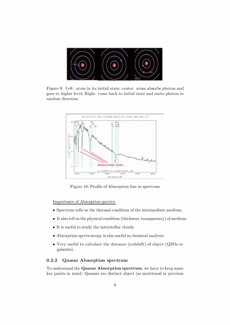
Figure 9: Left: atom in its initial state; center: atom absorbs photon andgoes to higher level; Right: come back to initial state and emits photon inrandom direction

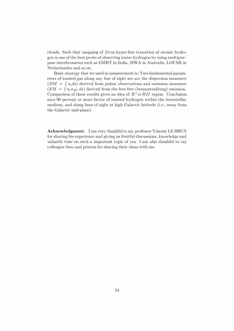
Figure 10: Profile of Absorption line in spectrum

Importance of Absorption spectra:

• Spectrum tells us the thermal condition of the intermediate medium.

• It also tell us the physical condition (thickness, transparency) of medium.

• It is useful to study the interstellar clouds.

• Absorption spectroscopy is also useful in chemical analysis.

• Very useful to calculate the distance (redshift) of object (QSOs orgalaxies).

0.2.2 Quasar Absorption spectrum

To understand the Quasar Absorption spectrum, we have to keep somekey points in mind: Quasars are distinct object (as mentioned in previous

6



report) and hydrogen is most abundant element in universe. So to classify

the spectrum we use hydrogen atom lines as our reference.Transition of electron in hydrogen atom first studied by Scientist Blamer,He classified when there is transition between nf = 2 to ni = 3, 4, 5, 6....lines are named as Hα,Hβ,Hγ and so on till Greek alphabet. this seriesis named as Blamer series (for visible light). Wavelength of emitted photonmeasured by Rydberg formula:

1

λ = R(

1

n2f

− 1

n2i

)

Where R is Rydberg constant R = 1.097×107m−1 Likewise when transitionin between n

f = 1 to n

i = 2, 3, 4, 5, 6.... lines are named as Lα, Lβ, Lγ (this

spread in UV light, If we calculate the wavelength by Rydberg formula ).similarly other series found but they are not for our concern right now. Figshows the calculated wavelengths of these series by Rydberg constant.

Figure 11:

Since we know, Quasars are high energetic and most luminous object inuniverse, therefore they emits high energetic photons. When these high en-ergetic photons passes through IGM they excite the hydrogen atom’s mostinner shell as well as other shells. As a consequence absorption take place,and we see absorption lines in optical spectra (I am explaining visible spec-tra). But If we are talking about the optical spectra (visible light) thenthere should be only Balmer series but what we seen is there is Forest of absorption line towards Blue region. Fig shows Quasar spectra:

7



Figure 12:

In mid 20’s scientific community(SC) detected, there are Lyman-α linesshifted in spectra due to high dispersion velocity (high red-shift Z). Butnow Question is how did SC measured that lines are shifted ? Thisfig shows, How do we measure that our Spectrum is shifted. Basically wecalibrate our taken spectra with standard star(the star very near (visually)to the quasar and at rest w.r.t. earth (not red-shifted)) we can measuredispersion velocity by

σv

C =

∆λ

λe

Where σv is dispersion velocity, delta lambda is difference between observedand emitted wavelength. lambda emitted is wavelength emitted at rest.

Figure 13: Upper spectrum strip show when star or cloud is moving we havelines little bit shifted from second spectrum strip which is taken at rest

And 1 + z = λoλe

Ref:(astro.ucla.edu) generally we have 1 + z = ∆λλe

8



0.2.3 Some Important calculations from ABSORPTION SPEC-

TRA:• we can deduced the red-shift(by Doppler effect), distance(Hubble

Law), recessional velocity, dispersion velocity as mentioned in aboveformulas.

• we can find out temperature, energy , specific Intensity etc by usingPlank’s energy distribution law and wein’s approximation.

• we can also measure the COLUMN DENSITY of cloud. Suppose beamof quasar light with an initial intensity I o traveling in the x directionalong our line of sight, and passing through the IGM gas cloud of thick-

ness L. We can say rate of change of intensity is I (x) is negative andis proportional to both the number density n(x) of absorbing atomsand initial density. Then we can write radiative transfer equation :

dI (x)

dx = −αλn(x)I o

where we define αλn(x)dx is optical depth τ λ of cloud. If we integrateoptical depth over the length L, then we can calculate column densityof absorbing cloud.

τ λ = αλ

L0

n(x)dx

τ λ = αλN

Where N is the column density along the line of sight. This is veryimportant feature that we can calculate by Quasar’s absorption spec-tra. By calculating this we can tell the type of absorption line thus,physical and chemical conditions of clouds: Just for little hint:

Lα forest clouds: If in IGM 1012cm−2 ≤ N (HI ) ≤ 1.6 ∗ 1017cm−2.Lyman-limit systems: If Gas clouds with N (HI ) ∼ 1.6∗1017cm−2

produces a stronger line in the Lα forest at wavelength 1261 A.sub-damped Lα system : N (HI ) ∼ 1019cm−2

Damped Lα system : N (HI ) > 2

∗1020cm−2

Line broadening, If absorbing atoms or molecules are in motion thenthere is broadening due to Doppler effect on observed wavelength. Sinceatoms in IGM has thermal velocity along LOS. We can assume Maxwelldistribution of velocities to find out distribution of atoms in interested area,therefore atoms will have gaussian distributed velocities along any compo-nent. This gives a Gaussian line profile for doppler broadening

φDoppler = 1

∆ν D√

π exp

−(ν − ν o)2

(∆ν D)2

9



where

∆ν D = ν o

c

2kBT

mH

It should be noted that the Doppler broadening of the lines is not due tothermal motions in the gas, but is also sensitive to any difference in velocitiesacross the absorbing cloud as a whole. For example, a Lα forest cloud that isfollowing the Hubble expansion will have some differential Hubble flow alongthe length of the cloud which would contribute to the Doppler broadening.Therefore total broadening will be :

φν = φnat × φDopp

• We can also detect metals and other components easily by lookingthe Profile of lines. If we refer above equations then we can say thatmetal lines will have a lower doppler width than hydrogen lines. Since,Atoms of other elements will have a mass greater than mH , so we willhave a lower thermal velocity, that will produce narrower absorption.lines.

0.3 Understanding the spatial distribution

Spectral analysis depend on the two technical factors of Telescope: Spectral

resolution and signal to noise ratio. Analysis says that with the low reso-lution spectrum, we can determine mean absorption and equivalent width.With Intermediate Resolution Spectroscopy we can count number of linesand with high resolution spectra it is possible to do all kind of science e.g.line profile fitting, number of lines, equivalent width and number density of HI and so on. In next few section I will discuss about all these propertieswith there spectral types.

0.3.1 Low Resolution Spectroscopy

In 1965 Gunn and Peterson defined mean absorption concept between Ly−αand Ly

−β lines. Now we called this as Gunn and Peterson effect to calculate

the mean absorption DA

DA = 1 − I

I o(1)

When we get spectra we simply follow the "radiation transfer law". Con-sider if I o is the initial intensity of light beam that passes through a gas cloudof length r and after passing through gas cloud we observe the intensity I then we can write Radiative transfer equation:

dI

dr = −αλI + J λ

10



where αλ = absorption − coefficient and J λ = emission − coefficient if

we consider we are looking on line of sight and cloud is totally homogeneousthen we will see only absorption in spectrum there for J λ = 0. and

dI

dr = −αλI

I I o

dI

I =

Lo−αλdr

I = I o exp(−τ λ) (2)

where αλdr = dτ λ is called optical depth of cloud. we define absorbencyof cloud mathematically by writing

αλ =

(cross sectional area of particle)×(volume inside)×(velocity of particles)dr

If we say cross-sectional-area-of-particle is σλ, particle-density (volume/area)is n and velocity is dl

dz then we can rewrite equation again like:

τ λ =

σλn(r)

dl

dzdr (3)

Where we scientifically say dldz is co-moving velocity of particles inside the

cloud. This we can calculate by online cosmological calculator by knowingthe red-shift.

Integration of n(r) over dr gives us COLUMN DENSITY of particles

per meter square. From equation (2) we can see if we know the observedintensities we can know the abundance (column density) of particles in cloud.

ln I

I o= exp(−σλ)vNHI (4)

Equation(4) is one of the most important physical quantity that we canmeasured from low-resolution spectra.

From equ(1) Mean Absorption is now:

DA = 1 − exp(−τ eff )

This is only called equivalent width of absorption spectral line.Conclusion: eauation (1) and (4) provide us physical quantities from

low-resolution spectroscopy.

0.3.2 Intermediate Resolution Spectroscopy

When we have little better resolution in spectrum then we can try to calcu-late the distribution of lines in spectrum this is called line counting. we doit simply by taking total length of spectra over the line width and red-shift(1+z) factor. 1+z factor is usually effected by power law. therefore d2L

dwdz =total no. of lines in certain length. This is one of the important quantitythat allow us to calculate the clumpiness of Ly − α forest.

11



0.3.3 High Resolution Spectroscopy

When we work on high resolution spectrum its easy to find all minute detailsand we find more and more factors that effects spectrum and there trans-parency. When we see in LRS we finds linearity in absorbency but when wego to HRS, we find its no more linear but that dose not mean calculationdone by LRS is wrong. They are exactly correct but with less features andwith HRS we finds more features. Like when we measures the optical depthwe found now αλ has dependence on broadening in lines.

αλ ∝ φ

Where φ is called broadening factor. There are two specific region for this

broadening first comes due to Quantum mechanical effect and second dueto Doppler effect. Quantum mechanical effect: In Q-mech we knowexcited electron can stay in upper energy levels for few seconds only, andby Heisenberg uncertainty principle ∆E∆T ∼ h and this uncertainty inthe energy calculated by Lorentzain. This broadening is known as Natural

broadening or Lorentzain broadening, given by:

φnat = 1

π

δ kδ (k2) + (ν − ν o)2

(5)

where

δ k =

1

4π

Akm

In this Akm is the Einstein coefficient gives the probability of spontaneoustransition of per particle per second from k (upper level) to m (lower level).

Doppler effect:If absorbing atoms or molecules are in motion then thereis broadening due to doppler effect in observed wavelength. Since atoms inIGM has thermal velocity along LOS. We can assume Maxwell distributionof velocities to find out distribution of atoms in interested area, thereforeatoms will have gaussian distributed velocities along any component. Thisgives a Gaussian line profile for Doppler broadening.

φDoppler =

1

∆ν D√ π exp −(ν

−ν o)2

(∆ν D)2

where

∆ν D = ν o

c

2kBT

mH

It should be noted that the Doppler broadening of the lines is not dueexclusively to thermal motions in the gas, but is also sensitive to any dif-ference in velocities across the absorbing cloud as a whole. For example, a

12



Lα forest cloud that is following the Hubble expansion will have some dif-

ferential Hubble flow along the length of the cloud, which would contributeto the Doppler broadening and also quantum mechanical effect would haveto taken in account. Therefore total broadening will be the convolutionproduct of these two effects. And we can rewrite equation of broadening :

φν = φnat ⊗ φDopp

Figure 14: Lorentzain and doppler broadening curves

After convolution of two function we get and average function calledVOIGT function this provides us and average Gaussian fit. shown inbelow figures. This gives us perfect estimation of spectrum’s physical quan-tities quantities.

13



Figure 15: fitted voigt function

Now, since we know the approximately correct line profile so we caneasily measure the dispersion velocity.

σv

C =

∆λ

λe(6)

Where σv is dispersion velocity, delta lambda is difference between observedand emitted wavelength. lambda emitted is wavelength emitted at rest.

0.3.4 Some other Important calculations from QSO absorp-tion spectra:

• we can deduced the red-shift(by Doppler effect), distance(HubbleLaw), recessional velocity, dispersion velocity as mentioned in aboveformulas.

• we can find out temperature, energy , specific intensity etc by using

Plank’s energy distribution law and wein’s approximation.

0.4 How to study Ly-alpha absorption line

0.4.1 Introduction

As we seen from observations in Inter galactic medium (IGM) neutral hy-drogen produces forest of Ly-alpha lines blue-ward in observed spectrum.This unique property of Quasar spectrum proves it as a considerable toolfor today’s cosmology. Observation of quasar beyond z > 2 shows there is

14



strong cosmological evolution in the number of ly-alpha lines which can be

characterized as a power law [sergent et.al]

dN

dz = N o(1 + z)γ (7)

In this my target is to explain observational studies with theoretical cos-mology and findout the gamma factor in theoretically and observationally.Furthermore, make a brief study on gamma factor and see why this gammafactor does not follow standard cosmology. Which factor is evolving gammaand which kind of physics we can study from this correction.

0.4.2 Theoretical Calculation

To explain all above I will use simple TOY MODEL of cosmology. In whichwe consider universe is homogeneous and isotropic, therefore there is spher-ical symmetry. In this we had taken a spherical cloud with :

• one characteristic size

• constant physical density

• Ω = Ω Λ + Ω m + Ω k + Ω R = 1

• Ω Λ = 0.7

• Ω m = 0.3

• Ω k = Ω R = 0

• physical distance is the function of z (red-shift) all these functions hasusual cosmological meaning,

In this section my target is to form cosmological equation for dN dz and

find-out gamma factor theoretically. We know N is the no. of absorptionlines, which is the function of optical depth i.e. the function of distance.Thus derivative of dN

dz gives us the column density with in the range z andz + dz.

dN

dl

dl

dzdN dz = No. of lines per unit length known as density so called column

density. Which can easily written as n(z).σ(z)dldz = derivative of co-moving distance with in the range z to z + dz

In toy model co-moving distance is given by

dl = c

H o(1 + z)

dz

E (z) (8)

15



where

E (z) =

Ω m(1 + z)3 + Ω k(1 + z)2 + Ω Λ

which is known as time derivative of logarithmic scale factor with respect tored-shift and other cosmological parameters.therefore

dN

dz =

dN

dl

dl

dz = n(z).σ(z)cH −1

o (1 + z)−1E (z) (9)

dN


o (1 + z)1/2 (10)

therefore theoretically γ = 0.5Figure Represent the graphical view of equation(3) by using considered

values of omega with different-different conditions:

Figure 16:

0.4.3 Observational calculation

By taking the reference of Kim et al. 1997 and willinger et al. 1994. Weseen in observational studies in high resolution spectroscopy for 2 < z < 3.5,γ = 2.78 ± 0.71 and γ > 4 for z > 4. In low resolution spectroscopyγ = 0.48 ± 0.62.

Since gamma is not equal 0.5, this clearly verify us, Ly-alpha forest in quasarspectra is not due to cosmological effect. There is some other factor thatis evolving. To understand this ambiguity scientific community has done somany simulation. one of the famous simulation is "Smooth particle hydro-dynamic simulation". This simulation has given us satisfactory results tounderstand evolving factor.In this simulation, cold dark matter (CDM) dominated universe has beenproduced Ly-alpha forest in the red-shift range 2 to 4 successfully. Fromsimulation we concluded:

16



• NHI column density was ≤ 1014cm−2 which produces weaker absorp-

tion lines in spectrum.

• Stronger absorption lines are shown in the region where NHI is ≤1016cm−2

• Velocity structure in lines are due to Hubble flow.

Therefore the smooth particle hydrodynamics simulation of CDM dominatemodel of universe has presented the impressive result of Ly-alpha forest prop-erties, and clarify the factor that is evolving, ’column density’ distribution,so called called no. of clouds on line of sight (LOS).

Figure 17: simulation and observed density comparision

Above fig Ref: Tom thuens et.al, fig shows there is column density evolu-tion with red-shift, and has good agreement between observed and simulatedcolumn density distribution at redshift z = 3 to 2

0.4.4 Discussion:

Below figure shows the comparison for different column density and simu-lation and result is extremely interesting. For different column density fitsare fitting the cosmology simulation but with different order. If we look ony axis limit we can see exactly that the order of variation of power law.

17



Figure 18: fig shows variation in order of gamma for different NHI

In figure 4, I am trying to plot the distribution of cloud and fit thesimulation model for low red-shift(red curve) and high red-shift(green curve).with this curve , I understood there is normalization factor and columndensity factor that varies. That is why fit is not perfect.

Figure 19:

After understanding with playing simulation I conclude that: Observa-tion explains, in IGM neutral hydrogen is only one percent and remaininghydrogen is in ionized form. We know Ly-alpha occur at when ground statehydrogen atom jumps to higher state. Ionized hydrogen has no electron soit does not absorb any photons. But in 2001 Becket et. al first confirmedthe Gunn-peterson(GP) effect in quasar spectrum, in this at some part of quasar spectra flux was zero. Since in IGM most of hydrogen is ionized,therefore the conclusion comes such kind of absorption in spectrum is dueto inter stellar medium (ISM) instead of IGM absorbent. We seen thesetroughs (where the flux zero) not only in single quasar of particular line

18



of sight but this effect is shown in every line of sight. The average optical

depth is steadily grows as we go further and its much more at z 6. Herewe conclude that this rising optical depth is due to rise in neutral hydrogenbeyond z > 6.- At the beginning of the universe all matter is not ionized and there werestrongly coupled photons in matter.- As the universe expand and cooled adiabatically, electron become boundto photons photons(CMB) released and matter and radiation decoupled.- At some point universe get re-ionized again and most of the neutral hy-drogen ionized

By studying quasar spectra we can conclude that when re-ionizationcompleted. The idea is very simple, If we could observe farther and farther

quasar, then we can calculate the red-shift where the quasar source is emit-ting. Since quasar is emitting means re-ionization completed, and it willstart showing GP effect intermediate clouds.

0.4.5 Conclusion:

By studying Quasar spectra by comparing cosmological model. We couldable to understand the structure of universe at large scale. we can calculatethe age of re-ionization era, IGM properties, presence of neutral hydrogenin ISM and presence of ionized hydrogen in IGM.

0.5 Calculation of absorbers size

In the observed spectrum, the ratio between two wavelength is always pre-served. This is very specific property to keep in mind (when we analyzespectrum). By this way we analyze the specific line s in spectrum. In prac-tice for example, we find doublet ratio of CIV (1548 A and 1551 A) andMgII (2796 A and 2803 A) in laboratory frame. If we find same ratio likethese lines then we predict the presence of particular absorver. After lookingon several spectrum of quasars scientific community standardize the classesof these absorvers. These absorvers are MgII, CIV, neutral hydrogen andclasses are defined by following:

N (MgII ) = 1016to1017cm−2

N (CIV ) = 1014to1016cm−2

N (HI ) = 1017to1020cm−2

Neutral hydrogen classes are defined in other sub classes but two mostspecific are: sub-damped Lα system N (HI ) ∼ 1019cm−2

Damped Lα system N (HI ) > 2 ∗ 1020cm−2

19



After finding lines by using ration of wavelength, we use co-relation func-

tion between these lines and we drive recessional velocity in the frame of ob-serving material. We typically find it 600km-1, that declare the signature of galaxies. By following this we could interpret that each cloud of particularclass is related to one galaxy. [reference: "Galaxies and cosmology" by ByFrancoise COMBES, Patrick Boissé, Alain]

So after this interpretation every things becomes very simple. since,If each cloud is one galaxy and we have distribution function of galaxies,so-called "galaxy luminosity function". It is defined by following:

φ(L)dl = φ∗ L

L∗exp(

−L

L∗)dl (11)

where φ∗ is normalization factorL = luminosity of galaxies L∗ = threshold luminosity

From the standard model of cosmology (discussed in previous report) weknow the column density distribution function, this is given by:

dN


o (1 + z)1/2 (12)

In equation(11) normalization function tells the no. of galaxies per cubicMpc. If we take a simple argument then we can say, this normalization factoris equivalent to the no. of particles per cubic Mpc. Therefore this argumentsimplifies :

φ∗ = n(z)

Then in equation(2) if we know the values of dN dz for particular classes

then we can easily drive cross-section of each object class.

σ(z) = dN (class)

dz

H oc

(1 + z)−1/2 1

φ∗M pc2 (13)

where,φ∗ = 1.6× 10−2h3

oM pc−3 and ho = H o100 (ref1)

H o = 70km/sec/Mpcc = 3

×105km/sec

0.5.1 Results

1. MgII absorbers:

At z<=2, dN (MgII )dz = 0.014[Ref: D’apre’s zhi-fu chen: "the red-shift num

density of MgII absorption systems"] we find values of cross-section σ(z) ∼101.02kpc. this value is quite considerable and I could find it in literature.

2. CIV absorbers:

20



At z= 1.5 to 3.5, dN (CIV )dz = 2.3 − 1.1 respectively [Ref: Nicolas tejos, "in-

dices of CIV on the line of sight"] and I found 148.34 kpc < σ(z) < 312.31kpc.

2. NHI absorbers:calculation of NHI is so weird, they are not as expected because columndensity of NHI absorbers are evolve as redshift increase or decreases (dis-

cussed in last report). At z<=0.1 - 2, dN (MgII )dz = 200− 50.11 respectively

[Ref: R.Dave "low redshift ly-alpha forest in cold dark matter" (z = 2)] [Ref:J. Michqel shull "low redshift intergalactic medium"(z = 0.1)] and I found2839.5 kpc < σ(z) < 1456.1 kpc.

2. Damped Ly-lapha absorbers:z<= 2.5, 0.16<dN (MgII )

dz < 0.25 [Ref: "K.Subramanian and T. Padman-abhan"] on the basis of this I found cross-section of 60 kpc < σ(z) < 75.3kpc.

21



0.6 Discussion

1: What are the three main global ionization era of the gaseouscomponent of the Universe, indicate for each what is the physicalphenomenon at the origin of the transition ?

After the Bigbang, for its first 370,000years the universe was filled withhot dense gas of plasma (ionized gas), photons were unable to escape fromsuch conditions. As the universe is keep on expanding and getting cool con-sequently electron and proton were able to combine and first neutral atom(hydrogen) form and photon were able to move freely in universe. Thesephotons was highly energetic and they travel through all universe, since uni-verse is keep on expanding, therefore high energy photons get shifted by

factor of 1000 and we see today them as CMB photons.Over the time, areas of high density regions began to collapse under

gravity, neutral matter in the universe began to clump together. Thus grav-ity and pressure counter-reaction force ignite nuclear fusion in the core of clumps and lead to first star and galaxy. As the first star emerged, thereenergy start heating the surrounding medium (photo-dissociation) and onceagain ionize the hydrogen of universe. As first galaxy emerged it is alsoeffected by associated radiative background.

Therefore the physical phenomenon happen at the origin of transitionare: Recombination by which first atom formed in universe, Gravity andpressure in-fall (jeans mass instability) by which first star and galaxy form,

Photo-dissociation from star and galaxy core that again leads neutral hy-drogen to ionized form.

2: What are the methods used to measure the physical size of Lyman alpha forest clouds at intermediate red-shifts (1 to 3), andwhat is this size

We know, Lyman-alpha clouds are every where and Quasar (QSO) spec-trum gives the finger prints of them. For calculating the size of Lyman-alpha

forest clouds, closely separated QSO pairs and gravitationally lensed QSOsprovides an efficient way. Gravitationally lensed QSOs has spatial separationof approx sub galactic scale. Therefore these QSOs provides two or more ad-

jacent ray path that can penetrate same cloud at different different positionsthen by statistical measurement (for example: Robust bayesian statisticalmethod in spherical and thick disk) on the absorbency of Ly-alpha, We con-clude the size of QSO. From the recent discoveries, lyman-alpha cloud hadsize 100 h−1kpc (measured from this method) [Ref: Yihu Fang et al.]

Another method is by using galaxy distribution function and objectclasses (discussed in section 0.5 (previous section)).

22



3: What is the average ionized gas fraction present in theseclouds?

At z = 3 fraction of neutral hydrogen is 10−5, If we follow the symme-try then I found 99.99 percent of ionize gas is available in these clouds. Itmeans almost everything is ionize.

4: At redshift > 3, which fraction of the baryons is containedin the Lyman alpha forest ?

Star and there remnants provides a very small contribution in the baryonicmass, while at z = 3 most of baryons are in intergalactic medium (IGM)in form of Lyman-alpha forest gas and damped lyman-alpha absorbers (inhigh density). Remaining part is in the form of cool plasma in betweenforest clouds. Observations measured number of baryons at red-shift z > 3is distributed in this ratios:

1. 60 percent in IGM

2. 7 percent in galaxies

3. 4 percent in clusters

4. 5 percent in circum-galactic gas

therefore total 80 percent baryons are available at z > 3.

5: In the present Universe, there is a large fraction of the in-tergalactic medium that cannot be detected through Lyman alphaabsorption, explain why, describe the physical state of this gas andthe observing strategies that have been used to detect it?

IONIZED HYDROGEN (HII) medium is the one that we can not detectfrom through lyman-alpha absorption. At z ∼ 6 heavy radiations, thosecomes from star and galactic center (QSO) ionize the neutral hydrogen of surrounding medium. Since it is ionized therefore no electron consequentlyno electron transition, Thus we can not observe such medium in absorp-tion spectrum. Observations at radio wavelengths are very interesting forHII. Due to photo-dissociation process these regions are highly energeticand emits high frequencies. These regions typically emit synchrotron andbremsstrahlung radiation at these frequencies, therefore provide us an ex-cellent independent probe of the temperatures and electron densities in the

23



clouds. Such that mapping of 21cm hyper-fine transition of atomic hydro-

gen is one of the best probe of observing ionize hydrogen by using multipur-pose interferometes such as GMRT in India, MWA in Australia, LOFAR inNetherlander and so on.

Basic strategy that we used in measurement is: Two fundamental param-eters of ionized gas along any line of sight are are the dispersion measures(DM =

neds) derived from pulsar observations and emission measures

(EM =

nenH +ds) derived from the free-free (bremsstrahlung) emission.Comparison of these results gives an idea of H +orHII region. Conclusionsays 90 percent or more factor of ionized hydrogen within the interstellarmedium, and along lines of sight at high Galactic latitude (i.e., away fromthe Galactic mid-plane)

Acknowledgment: I am very thankful to my professor Vincent LE BRUNfor sharing his experience and giving us fruitful discussions, knowledge andvaluable time on such a important topic of era. I am also thankful to mycolleague theo and priston for sharing their ideas with me.

24



0.7 References

[1] http : //www.astronomynotes.com/galaxy/s14.htm[2] http : //www.astronomy.ohio−state.edu/ ryden/ast1628/notes36.html[3] http : //skyserver.sdss.org/dr1/en/proj/advanced/quasars/power.asp[4] http : //www.astro.washington.edu/users/ivezic/REU 08/quasarweb/background/basic 1.html[5] http : //www.atnf.csiro.au/outreach/education/senior/astrophysics/spectra[6] Quasar Absorbers and the InterGalactic Medium Simon C. Reynolds .pfd[7] http : //spiff.rit.edu/classes/phys301/lectures/speclines/speclines.html[8] http : //astrobites.org/guides/spectroscopy − and− spectral − lines/[9] http : //w.astro.berkeley.edu/ ay216/08/NOTES/Lecture26 − 08.pdf [10] https : //ned.ipac.caltech.edu/level5/Charlton/Charlton11.html

[11]David W. Hogg, Institute for Advanced Study, 1 Einstein Drive, Prince-ton NJ 08540[12]The low-redshift evolution of the Ly-alpha Forest by Tom Theuns et.al[13] Sargent and Peter J et. al[14] http : //astrobites.org/2013/07/21/astrophysical−classics−neutral−hydrogen−in−the−universe− part−2/ [15] https : //www.astro.umd.edu/ richard/AST RO620/Lu

pp.pdf (normalization factor)[16] Basic understanding of absorbers by churchill http : //astronomy.nmsu.edu/cwc/Research/MgI review/mgii− over.html − gal − stats[17] D’apre’s zhi-fu chen et.al[18] Nicolas tejos et.al

[19] R.Dave "low redshift ly-alpha forest in cold dark matter"[20] K.Subramanian et.al from TIFR[21] The evolution of the intergalactic medium by Matthew Mcquinn.[22] New horizons of observational cosmology by A. Cooray, E. Komatsu, A.Melchiorri.[23] The size and nature of Lyman-alpha forest clouds probed by QSO pairsand groups, Yihu Fang et al., astroph 9510112.

25

quasars with a cosmoloical approach

Documents