Quantum Theory of Condensed Matter

John ChalkerPhysics Department, Oxford University

2013

I aim to discuss a reasonably wide range of quantum-mechanical phenomena from condensed matter physics,with an emphasis mainly on physical ideas rather than mathematical formalism. The most important prerequisiteis some understanding of second quantisation for fermions and bosons. There will be two problems classes inaddition to the lectures.

Michaelmas Term 2013: Lectures in the Fisher Room, Dennis Wilkinson Building, Physics Department, onWednesdays at 10:00 and Fridays at 11:00.

OUTLINE

• Overview

• Spin waves in magnetic insulators

• One-dimensional quantum magnets

• Superfluidity in a weakly interacting Bose gas

• Landau’s theory of Fermi liquids

• BCS theory of superconductivity

• The Mott transition and the Hubbard model

• The Kondo effect

• Disordered conductors and Anderson localisation

• Anderson insulators

• The integer and fractional quantum Hall effects

1

wit

h U

(1)

sym

met

ry

Wea

k c

orr

elat

ions

Ov

eral

l sc

hem

e

Str

ong c

orr

elat

ions

Wea

k c

orr

elat

ions

Bo

son

sF

erm

ion

s

Idea

l B

ose

gas

Idea

l F

erm

i gas

BC

S s

uper

conduct

or

Lan

dau

ferm

i li

quid

Hubbar

d m

odel

+

Mott

insu

lato

r

Kondo

effe

ct

Ander

son i

nsu

lato

r

QH

E

Ord

ered

mag

net

Super

fluid

Str

ong

fluct

uat

ions

in 1

D

wea

kin

tera

ctio

ns

wea

kat

trac

tio

n

wea

k

rep

uls

ion

ran

do

m i

mp

uri

ty p

ote

nti

al

rep

uls

ion

+p

erio

dic

lat

tice

mag

net

ic f

ield

in 2

D

Rep

uls

ion

at

on

e la

ttic

e si

te

Eq

uiv

alen

ce

2

Bibliography

Background

N W Ashcroft and N D Mermin Solid State Physics, Holt-Sanders (1976). I assume familiarity with thismaterial.

S-K Ma Statistical Mechanics, World Scientific (1985). Strongly recommended book at a level suitable forfirst year graduate students.

J-P Blaizot and G Ripka Quantum Theory of Finite Systems, MIT (1986). A very thorough treatment ofsecond quantisation, canonical transformations and self-consistent field approximations.

Recent Graduate Texts

A. Altland and B. D. Simons Quantum Field Theory in Condensed Matter Physics, CUP (2006). An acces-sible introduction to the subject.

S. Sachdev Quantum Phase Transitions, CUP (1999).An advanced survey of theoretical approaches to this subject.

H. Bruus and K. Flensberg Many Body Quantum Theory in Condensed Matter Physics, OUP (2004).A detailed introduction to techniques and a discussion of topics of current interest, especially in connectionwith mesoscopic conductors and quantum dots.

X.-G. Wen Quantum Field Theory of Many-Body Systems, OUP (2004). An outline of basic material fol-lowed by an introduction to some advanced topics (topological order, the fractional quantum Hall effect, andspin liquids).

A. M. M. Tsvelik Quantum Field Theory in Condensed Matter Physics, CUP (1995). A concise survey ofapplications of field theory to condensed matter problems, especially in one dimension.

A. Auerbach Interacting Electrons and Quantum Magnetism, Springer (1994).A reasonably gentle introduction to a range of current theoretical ideas.

General Texts

P W Anderson Concepts in Solids, Benjamin (1963). A classic introduction to solid state physics at agraduate level.

C Kittel Quantum Theory of Solids, Wiley (1963). [N.B. not the undergraduate text by the same author].Includes most of the material covered in the first third of the lecture course.

D. Pines and P. Nozieres The Theory of Quantum Liquids, Volume 1, Addison Wesley (1989). A standardaccount of Fermi liquids.

P W Anderson Basic Notions in Condensed Matter Physics, Benjamin (1984). When first published was anadvanced discussion of some of the most important ideas in the subject.

A. J. Leggett Quantum Liquids, OUP (2006). A clear and wide-ranging discussion of Bose condensationand Cooper pairing.

3

Electrons in disordered conductors.

N F Mott Conduction in Non-Crystalline Materials O.U.P. (1987) For a survey.

P. A. Lee and B. I. Altshuler, Physics Today 41 36 (1988), and P.A. Lee and S-C Feng, Science 251 633(1991). Two accessible introductions to interference effects on transport in disordered media.

Y. Imry Introduction to Mesoscopic Physics O. U. P. (1997). Also an article in Directions in Condensed Mat-ter Physics, Edited by G. Grinstein and G Mazenko, World Scientific (1986). A more advanced discussion,but in the same spirit as Lee and Altshuler’s article.

Some consequences of electron-electron interactions.

N F Mott Metal Insulator Transitions, Taylor and Francis (1990), and A. C. Hewson The Kondo Problem toHeavy Fermions Cambridge (1993). Two complementary reviews.

The Quantum Hall Effect.

R. E. Prange and S. M. Girvin The Quantum Hall Effect, Springer (1990). A standard introduction, nowrather old.

S. M. Girvin The Quantum Hall Effect: Novel Excitations and Broken Symmetries Lectures delivered atEcole d’Ete Les Houches, July 1998; cond-mat/9907002A more recent review of quantum Hall physics.

Green functions, response functions and perturbation theory

A. A. Abrikosov, L. P. Gorkov and I. E. Dzyaloshinski Methods of quantum field theory in statistical physics,Dover (1975). Still possibly the best starting point.

A. L. Fetter and J. D. Walecka Quantum Theory of Many-Particle Systems, McGraw-Hill, (1971); alsoavailable from Dover. A standard and straightforward introduction.

J. W. Negele and H. Orland Quantum Many-Particle Systems, Addison Wesley (1987). A modern treatmentbased on path integrals.

G. D. Mahan Many-Particle Physics, Plenum (1990).A very detailed treatment of Green function techniques in many body theory.

4

Many-Particle Quantum Systems

1 Identical particles in quantum mechanicsMany-particle quantum systems are always made up of many identical particles, possibly of several different kinds.Symmetry under exchange of identical particles has very important consequences in quantum mechanics, and theformalism of many-particle quantum mechanics is designed to build these consequences properly into the theory.We start by reviewing these ideas.

Consider a system ofN identical particles with coordinates r1, . . . rN described by a wavefunctionψ(r1 . . . rN ).For illustration, suppose that the Hamiltonian has the form

H = − ~2

2m

N∑i=1

∇2i +

N∑i=1

V (ri) +∑i<j

U(ri − rj) .

Here there are three contributions to the energy: the kinetic energy of each particle (∇2i operates on the coordinates

ri); the one-body potential energy V (r); and the two-particle interaction potentialU(ri−rj). To discuss symmetryunder exchange of particles, we define the exchange operator Pij via its action on wavefunctions:

Pijψ(. . . ri . . . rj . . .) = ψ(. . . rj . . . ri . . .) .

Since [H,Pij ] = 0, we can find states that are simultaneous eigenstates of H and Pij . Moreover, a system thatis initially in an eigenstate of Pij will remain in one under time evolution with H. For these reasons we examinethe eigenvalues of Pij . Since (Pij)2 = 1, these are +1 and −1. Now, it is an observational fact (explained inrelativistic quantum field theory by the spin-statistics theorem) that particles come in two kinds and that particlesof a given kind are always associated with the same eigenvalue of the exchange operator: +1 for bosons and −1for fermions.

1.1 Many particle basis statesIn a discussion of many-particle quantum systems we should restrict ourselves to wavefunctions with the appropri-ate symmetry under particle exchange. We can do this by using a set of basis states that has the required symmetry.As a starting point, suppose that we have a complete, orthonormal set of single-particle states φ1(r), φ2(r) . . ..Next we would like to write down a wavefunction representing an N -particle system with one particle in state l1,one in state l2 and so on. The choice

φl1(r)φl2(r) . . . φlN (r)

is unsatisfactory because for general l1, l2 . . . it has no particular exchange symmetry. Instead we take

ψ(r1 . . . rN ) = N∑

distinct perms.

(±1)Pφk1(r1) . . . φkN (rN ) . (1)

Several aspects of the notation in Eq. (1) require comment. The sign inside the brackets in (±1)P is +1 for bosonsand −1 for fermions. The set of labels k1 . . . kN is a permutation of the set l1 . . . lN. The permutation iscalled even if it can be produced by an even number of exchanges of adjacent pairs of labels, and is odd otherwise;the integer P is even or odd accordingly. The sum is over all distinct permutations of the labels. This means thatif two or more of the labels ln are the same, then permutations amongst equal labels do not appear as multiplecontributions to the sum. Finally, N is a normalisation, which we determine next.

To normalise the wavefunction, we must evaluate∫ddr1 . . .

∫ddrN ψ

∗(r1 . . . rN )ψ (r1 . . . rN ) .

Substituting from Eq. (1), we obtain a double sum (over permutations k1 . . . kN and h1 . . . hN ) of terms of theform ∫

ddr1 φ∗k1(r)φh1

(r1) . . .

∫ddrN φ

∗kN (r)φhN

(r1) .

5

These terms are zero unless k1 = h1, k2 = h2, and . . . kN = hN , in which case they are unity. Therefore only thediagonal terms in the double sum contribute, and we have∫

. . .

∫|ψ|2 = |N |2

∑dist. perms.

(±1)2P = |N |2 N !

n1!n2! . . .

where the n1, n2 . . . are the numbers of times that each distinct orbital appears in the set l1 . . . lN, and the ratioof factorials is simply the number of distinct permutations. Hence we normalise the wavefunction to unity bytaking

N =

(n1! n2! . . .

N !

)1/2

.

1.2 Slater determinantsFor fermion wavefunctions we can get the correct signs by thinking of Eq. (1) as a determinant

ψ(r1 . . . rN ) =1√N !

∣∣∣∣∣∣φl1(r1) . . . φl1(rN)

. . .φlN (r1) . . . φlN (rN)

∣∣∣∣∣∣ . (2)

Note that this determinant is zero either if two orbitals are the same (li = lj) or if two coordinates coincide(ri = rj), so the Pauli exclusion principle is correctly built in. Note also that, since the sign of the determinant ischanged if we exchange two adjacent rows, it is necessary to keep in mind a definite ordering convention for thesingle particle orbitals φl(r) to fix the phase of the wavefunction.

For bosons, we should use an object similar to a determinant, but having all terms combined with a positivesign: this is known as a permanent.

1.3 Occupation numbersWe can specify the basis states we have constructed by giving the number of particles nl in each orbital l. Clearly,for fermions nl = 0 or 1, while for bosons nl = 0, 1, . . .. These occupation numbers are used within Dirac notationas labels for a state: |n1, n2, . . .〉.

1.4 Fock spaceCombining states |n1, n2, . . .〉 with all possible values of the occupation numbers, we have basis vectors for stateswith any number of particles. This vector space is known as Fock space. Using it, we can discuss processes inwhich particles are created or annihilated, as well as ones with fixed particle number, described by wavefunctionsof the form ψ(r1 . . . rN ).

1.5 The vacuum stateIt is worth noting that one of the states in Fock space is the vacuum: the wavefunction for the quantum systemwhen it contains no particles, written as |0〉. Clearly, in recognising this as a quantum state we have come someway from the notation of single-body and few-body quantum mechanics, with wavefunctions written as functionsof particle coordinates. Of course, |0〉 is different from 0, and in particular 〈0|0〉 = 1.

1.6 Creation and annihilation operatorsMany of the calculations we will want to do are carried out most efficiently by introducing creation operators, whichadd particles when they act to the right on states from Fock space. Their Hermitian conjugates are annihilationoperators, which remove particles. Their definition rests on the set of single particle orbitals from which we builtFock space: c†l adds particles to the orbital φl(r). More formally, we define

c†l1c†l2. . . c†lN |0〉 (3)

to be the state with coordinate wavefunction

ψ(r1, . . . rN ) =1√N !

∑all perms

(±1)Pφk1(r1) . . . φkN (rN ) = (n1!n2! . . .)1/2|n1, n2 . . .〉 . (4)

6

A detail to note is that the sum in Eq. (4) is over all permutations, while that in Eq. (1) included only distinctpermutations. The difference (which is significant only for bosons, since it is only for bosons that we can havenl > 1), is the reason for the factor (n1!n2! . . .)1/2 appearing on the right of Eq. (4). This choice anticipates whatis necessary in order for boson creation and annihilation operators to have convenient commutation relations.

Annihilation operators appear when we take the Hermitian conjugate of Eq. (3), obtaining 〈0| clN . . . cl2cl1 .Let’s examine the effect of creation and annihilation operators when they act on various states. Since c†l |0〉 is thestate with coordinate wavefunction φl(r), we know that 〈0|cl c

†l |0〉 = 1, but for any choice of the state |φ〉 other

than the vacuum, c†l |φ〉 contains more than one particle and hence 〈0|cl c†l |φ〉 = 0. From this we can conclude that

cl c†l |0〉 = |0〉 ,

demonstrating that the effect of cl is to remove a particle from the state |nl=1〉 ≡ c†l |0〉. We also have for any |φ〉the inner products 〈0|c†l |φ〉 = 〈φ|cl |0〉 = 0, and so we can conclude that

cl |0〉 = 〈0|c†l = 0 .

1.7 Commutation and anticommutation relationsRecalling the factor of (±1)P in Eq. (4), we have for any |φ〉

c†l c†m|φ〉 = ±c†mc

†l |φ〉 ,

where the upper sign is for bosons and the lower one for fermions. From this we conclude that boson creationoperators commute, and fermion creation operators anticommute: that is, for bosons

[c†l , c†m] = 0

and for fermionsc†l , c

†m = 0 ,

where we use the standard notation for an anticommutator of two operatorsA andB: A,B = AB+BA. TakingHermitian conjugates of these two equations, we have for bosons

[cl, cm] = 0

and for fermionscl, cm = 0 .

Note for fermions we can conclude that (cl )2=(c†l )

2=0, which illustrates again how the Pauli exclusion principleis built into our approach.

Finally, one can check that to reproduce the values of inner products of states appearing in Eq. (4), we requirefor bosons

[cl , c†m] = δlm

and for fermionscl , c

†m = δlm .

To illustrate the correctness of these relations, consider for a single boson orbital the value of |[(c†)n|0〉]|2. FromEq. (4) we have |[(c†)n|0〉]|2 = n!. Let’s recover the same result by manipulating commutators: we have

〈0|(c)n(c†)n|0〉 = 〈0|(c)n−1([c, c†] + c†c)(c†)n−1|0〉= m〈0|(c)n−1(c†)n−1|0〉+ 〈0|c†(c)n−mc†c(c)m(c†)n−1|0〉= n〈0|(c)n−1(c†)n−1|0〉+ 〈0|c†(c)n−1(c†)n−1|0〉= n(n− 1) . . . (n− l)〈0|(c†)n−l(c)n−l|0〉= n! 〈0|0〉 .

Of course, manipulations like these are familiar from the theory of raising and lowering operators for the harmonicoscillator.

7

1.8 Number operatorsFrom Eq. (4) as the defining equation for the action of creation operators in Fock space we have

c†l |n1 . . . nl . . .〉 = (±1)n1+...+nl−1√nl + 1|n1 . . . nl + 1 . . .〉 ,

or zero for fermions if nl=1. Similarly, by considering the Hermitian conjugate of a similar equation, we have

cl|n1 . . . nl . . .〉 = (±1)n1+...+nl−1√nl|n1 . . . nl − 1 . . .〉 ,

or zero for both bosons and fermions if nl=0. In this way we have

c†l cl | . . . nl . . .〉 = nl| . . . nl . . .〉

where the possible values of nl are nl=0, 1, 2 . . . for bosons and nl=0, 1 for fermions. Thus the combination c†l cl ,which we will also write as nl, is the number operator and counts particles in the orbital φl.

1.9 Transformations between basesIn the context of single-particle quantum mechanics it is often convenient to make transformations between differ-ent bases. Since we used a particular set of basis functions in our definition of creation and annihilation operators,we should understand what such transformations imply in operator language.

Suppose we have two complete, orthonormal sets of single-particle basis functions, φl(r) and ρα(r),which we also write as |φi〉 and |ρα〉. Then we can expand one in terms of the other, writing

ρα(r) =∑l

φl(r)Ulα (5)

with Ulα = 〈φl|ρα〉. Note that U is a unitary matrix, since

(UU†)ml =∑α

〈φm|ρα〉〈ρα|φl〉

= 〈φm|φl〉 since∑α

|ρα〉〈ρα| = 1

= δml .

Now let c†l create a particle in orbital φl(r), and let d†α create a particle in orbital ρα(r). We can read off fromEq. (5) an expression for d†α in terms of c†l :

d†α =∑l

c†lUlα .

From the Hermitian conjugate of this equation we also have

dα =∑l

U∗lαcl =∑l

(U†)αlcl .

1.9.1 Effect of transformations on commutation relations

We should verify that such transformations preserve commutation relations. For example, suppose that cl and c†lare fermion operators, obeying cl , c†m = δlm. Then

dα, d†β =

∑lm

U∗lαUmβ cl , c†m = (U†U)αβ = δαβ .

Similarly, for boson operators commutation relations are preserved under unitary transformations.

8

1.10 General single-particle operators in second-quantised formTo continue our programme of formulating many-particle quantum mechanics in terms of creation and annihilationoperators, we need to understand how to transcribe operators from coordinate representation or first-quantised formto so-called second-quantised form. In the first instance, we examine how to do this for one-body operators – thosewhich involve the coordinates of one particle at a time. An example is the kinetic energy operator. Suppose ingeneral that A(r) represents such a quantity for a single-particle system. Then for a system of N particles infirst-quantised notation we have

A =

N∑i=1

A(ri) .

We want to represent A using creation and annihilation operators. As a first step, we can characterise A(r) byits matrix elements, writing

Alm =

∫φ∗l (r)A(r)φm(r)ddr .

ThenA(r)φm(r) =

∑l

φl(r)Alm . (6)

The second-quantised representation isA =

∑pq

Apqc†pcq . (7)

To justify this, we should verify that reproduces the correct matrix elements between all states from the Fock space.We will simply check the action of A on single particles states. We have

A|φm〉 =∑pq

Apqc†pcqc

†m|0〉 .

Now, taking as an example bosons,

c†pcqc†m|0〉 = c†p([cq, c

†m] + c†mcq)|0〉 = c†pδqm|0〉

soA|φm〉 =

∑p

|φp〉Apm ,

reproducing Eq. (6), as required.

1.11 Two-particle operators in second-quantised formTwo-body operators depend on the coordinates of a pair of particles, an example being the two-body potential inan interacting system. Writing the operator in first-quantised form as A(r1, r2), it has matrix elements which carryfour labels:

Almpq =

∫φ∗l (r1)φ∗m(r2)A(r1, r2)φp(r2)φq(r1)ddr1ddr2 .

Its second-quantised form isA ≡

∑ij

A(ri, rj) =∑lmpq

Almpqc†l c†mcpcq . (8)

Again, to justify this one should check matrix elements of the second-quantised form between all states in Fockspace. We will content ourselves with matrix elements for two-particle states, evaluating

〈A〉 = 〈0|cycxAc†ac†b|0〉

by two routes. In a first-quantised calculation with ± signs for bosons and fermions, we have

〈A〉 =1

2

∫ ∫[φ∗x(r1)φ∗y(r2)± φ∗x(r2)φ∗y(r1)] · [A(r1, r2) +A(r2, r1)] · [φa(r1)φb(r2)± φa(r2)φb(r1)]ddr1ddr2

=1

2[Axyba ±Axyab +Ayxab ±Ayxba +Axyba ±Axyab +Ayxab ±Ayxba]

= (Axyba +Ayxab)± (Axyab +Ayxba) . (9)

9

Using the proposed second-quantised form for A, we have

〈A〉 =∑lmpq

Almpq〈0|cycxc†l c†mcpcqc

†ac†b|0〉 .

We can simplify the vacuum expectation value of products of creation and annihilation operators such as the oneappearing here by using the appropriate commutation or anticommutation relation to move annihilation operatorsto the right, or creation operators to the left, whereupon acting on the vacuum they give zero. In particular

cpcqc†ac†b|0〉 = (δaqδbp ± δapδbq)|0〉

and〈0|cycxc

†l c†m = 〈0|(δymδxl ± δylδxm) .

Combining these, we recover Eq. (9).

2 Diagonalisation of quadratic HamiltoniansIf a Hamiltonian is quadratic (or, more precisely, bilinear) in creation and annihilation operators we can diagonaliseit, meaning we can reduce it to a form involving only number operators. This is an approach that applies directlyto Hamiltonians for non-interacting systems, and also to Hamiltonians for interacting systems when interactionsare treated within a mean field approximation.

2.1 Number-conserving quadratic HamiltoniansSuch Hamiltonians have the form

H =∑ij

Hija†iaj .

Note that in order for the operator H to be Hermitian, we require the matrix H to be Hermitian. Since the matrixH is Hermitian, it can be diagonalised by unitary transformation. Denote this unitary matrix by U and let theeigenvalues of H be εn. The same transformation applied to the creation and annihilation operators will diagonaliseH. The details of this procedure are as follows. Let

α†l =∑i

a†iUil .

Inverting this, we have ∑α†l (U

†)lj = a†j

and taking a Hermitian conjugate ∑l

Ujlαl = aj .

Substituting for a†’s and a’s in terms of α†’s and α’s, we find

H =∑lm

α†l (U†HU)lmαm =

∑n

εnα†nαn ≡

∑n

εnnn .

Thus the eigenstates of H are the occupation number eigenstates in the basis generated by the creation operatorsα†n.

2.2 Mixing creation and annihilation operators: Bogoliubov transformationsThere are a number of physically important systems which, when treated approximately, have bilinear Hamiltoni-ans that include terms with two creation operators, and others with two annihilation operators. Examples includesuperconductors, superfluids and antiferromagnets. These Hamiltonians can be diagonalised by what are known asBogoliubov transformations, which mix creation and annihilation operators, but, as always, preserve commutationrelations. We now illustrate these transformations, discussing fermions and bosons separately.

10

2.2.1 Fermions

Consider for fermion operators the Hamiltonian

H = ε(c†1c1 + c†2c2) + λ(c†1c†2 + c2c1) ,

which arises in the BCS theory of superconductivity. Note that λ must be real for H to be Hermitian (moregenerally, with complex λ the second term of H would read λc†1c

†2 + λ∗c2c1). Note as well the opposite ordering

of labels in the terms c†1c†2 and c2c1, which is also a requirement of Hermiticity.

The fermionic Bogoliubov transformation is

c†1 = ud†1 + vd2

c†2 = ud†2 − vd1 , (10)

where u and v are c-numbers, which we can in fact take to be real, because we have restricted ourselves to realλ. The transformation is useful only if fermionic anticommutation relations apply to both sets of operators. Let ussuppose they apply to the operators d and d†, and check the properties of the operators c and c†. The coefficientsof the transformation have been chosen to ensure that c†1, c

†2 = 0, while

c†1, c1 = u2d†1, d1+ v2d†2, d2

and so we must require u2 + v2 = 1, suggesting the parameterisation u = cos θ, v = sin θ.The remaining step is to substitute inH for c† and c in terms of d† and d, and pick θ so that terms in d†1d

†2+d2d1

have vanishing coefficient. The calculation is clearest when it is set out using matrix notation. First, we can writeH as

H =1

2

(c†1 c2 c†2 c1

)ε λ 0 0λ −ε 0 00 0 ε −λ0 0 −λ −ε

c1c†2c2c†1

+ ε

where we have used the anticommutator to make substitutions of the type c†c = 1− c c†.For conciseness, consider just the upper block

(c†1 c2

)( ε λλ −ε

)(c1c†2

)and write the Bogoliubov transformation also in matrix form as(

c1c†2

)(cos θ sin θ− sin θ cos θ

)(d1d†2

).

We pick θ so that (cos θ − sin θsin θ cos θ

)(ε λλ −ε

)(cos θ sin θ− sin θ cos θ

)=

(ε 00 −ε

),

where ε =√ε2 + λ2. Including the other 2× 2 block ofH, we conclude that

H = ε(d†1d1 + d†2d2) + ε− ε .

2.2.2 Bosons

The Bogoliubov transformation for a bosonic system is similar in principle to what we have just set out, butdifferent in detail. We are concerned with a Hamiltonian of the same form, but now written using boson creationand annihilation operators:

H = ε(c†1c1 + c†2c2) + λ(c†1c†2 + c2c1) .

We use a transformation of the form

c†1 = ud†1 + vd2

c†2 = ud†2 + vd1 .

11

Note that one sign has been chosen differently from its counterpart in Eq. (10) in order to ensure that bosoniccommutation relations for the operators d and d† imply the result [c†1, c

†2] = 0. We also require

[c1, c†1] = u2[d1, d

†1]− v2[d2, d

†2] = 1

and hence u2 − v2 = 1. The bosonic Bogoliubov transformation may therefore be parameterised as u = cosh θ,v = sinh θ.

We can introduce matrix notation much as before (but note some crucial sign differences), with

H =1

2

(c†1 c2 c†2 c1

)ε λ 0 0λ ε 0 00 0 ε λ0 0 λ ε

c1c†2c2c†1

− ε ,where for bosons we have used the commutator to write c†c = c c† − 1. Again, we focus on one 2× 2 block

(c†1 c2

)( ε λλ ε

)(c1c†2

)and write the Bogoliubov transformation also in matrix form as(

c1c†2

)(u vv u

)(d1d†2

).

Substituting for c and c† in terms of d and d†, this block of the Hamiltonian becomes

(d†1 d2

)( u vv u

)(ε λλ ε

)(u vv u

)(d1d†2

).

In the fermionic case the matrix transformation was simply an orthogonal rotation. Here it is not, and so we shouldexamine it in more detail. We have(

u vv u

)(ε λλ ε

)(u vv u

)=

(ε[u2 + v2] + 2λuv 2εuv + λ[u2 + v2]2εuv + λ[u2 + v2] ε[u2 + v2] + 2λuv

).

It is useful to recall the double angle formulae u2 + v2 = cosh 2θ and 2uv = sinh 2θ. Then, setting tanh 2θ =−λ/ε we arrive at

H = ε(d†1d1 + d†2d2)− ε+ ε .

withε =

√ε2 − λ2. (11)

Note that in the bosonic case the transformation requires ε > λ: if this is not the case, H is not a Hamiltonianfor normal mode oscillations about a stable equilibrium, but instead represents a system at an unstable equilibriumpoint.

2.3 Fourier transform conventionsWe will use Fourier transforms extensively, because much of the time we will be considering systems that aretranslation-invariant, and the plane waves used in these transforms are eigenfunctions of translation operators. Forconvenience, we collect here some definitions. Although we are generally interested in the thermodynamic limit(the limit of infinite system size), it is usually clearest and cleanest to write transforms in the first instance fora finite system. In order to preserve translation invariance, we take this finite system to have periodic boundaryconditions. Since some details differ, we consider lattice and continuum problems separately.

12

2.3.1 Lattice systems

Consider a three-dimensional Bravais lattice with basis vectors a, b, and c. Lattice sites have coordinates

r = la +mb + nc (12)

with l,m and n integer. Periodic boundary conditions mean that l + N1 ≡ l, m + N2 ≡ m, and n + N3 ≡ n,and the number of lattice sites is then N = N1N2N3. In the usual way, reciprocal lattice vectors G1, G2 and G3

satisfy G1 · a = 2π, G1 · b = G1 · c = 0 and so on. Then the wave eikr satisfies periodic boundary conditions if

k = 2π

(n1N1

G1,n2N2

G2,n3N3

G3

)(13)

with n1, n2 and n3 integer. Note that we have N values of k in the Brillouin zone.Let c†r be a (boson or fermion) creation operator at the site r. We define the Fourier transform and inverse

transform by

c†k =1√N

∑r

e−ikrc†r and c†r =1√N

∑k

eikrc†k . (14)

There are several points to make here. First, one should check for consistency by substituting one expression intothe other. Second, these definitions use the unitary N ×N matrix U, which has elements

Ukr =1√N

eikr .

Third, if we consider time-dependence in the Heisenberg picture with a HamiltonianH = ~ω(k)c†kck we have

c†k(t) ≡ eiHtc†ke−iHt = c†ke−iωkt and c†r(t) =1√N

∑k

ei[kr−ω(k)t]c†k ,

which has the usual traveling wave form.

2.3.2 Continuum systems

Consider a cube of side L and volume V with periodic boundary conditions. Take

k =2π

L(n1, n2, n3)

with n1, n2 and n3 integer. Then the wavefunctions

ψk(r) = V −1/2eikr

form a normalised single-particle basis.Let c†(r) be a (boson or fermion) creation operator for a particle at the point r. Then the creation operator for

a particle in the state with wavefunction ψk(r) is

c†k = V −1/2∫

d3r e−ikr c†(r) (15)

and the inverse transform isc†(r) =

1√V

∑k

eikrc†k . (16)

2.3.3 Thermodynamic limit

In the thermodynamic limit sums on wavevectors can be replaced by integrals. On a lattice we have

N−1∑k

→ 1

Ω

∫BZ

ddk , (17)

where the integral is over the Brillouin zone of volume Ω. In the continuum we have

V −1∑k

→ (2π)−d∫

ddk . (18)

13

Quantum Magnets and the Bose Gas

3 The Heisenberg modelWe move now to applying some of these ideas to the theory of magnetism. We will consider insulating magnets (asdistinct from itinerant ones, in which the electrons involved in magnetism belong to a partially-filled conductionband that has a Fermi surface). We model an insulating magnetic material using spin operators to represent mag-netic moments at the sites of a lattice. The formation of these magnetic moments can be understood in terms ofthe atomic physics of an isolated ion: we postpone discussion of this aspect to Section 6. Neighbouring magneticmoments are coupled by exchange interactions, and a simple model that captures this is the Heisenberg model. Wetake nearest neighbour interactions of strength J (where J > 0), and study the Hamiltonian

H = ±J∑〈rr′〉

Sr · Sr′ ≡ ±J∑〈rr′〉

[SzrS

zr′ +

1

2

(S+r S−r′ + S−r S

+r′

)]. (19)

Here∑〈rr′〉 denotes a sum over neighbouring pairs of sites on the lattice, with each pair counted once. With a

negative sign in front of J , parallel spins have lower energy and the system is a ferromagnet, while with a positivesign antiparallel spins are favoured and the system is an antiferromagnet.

The three components of spin at site r are represented by operators Sxr , Syr and Szr . Their commutation relationsare the standard ones, and with ~ = 1 take the form

[Sir1 , Sjr2 ] = iδr1,r2εijkS

kr1 .

We emphasise two points: first, the commutation relations are more complicated than those for creation and an-nihilation operators, since the commutator is itself another operator and not a number; and second, spin operatorsacting at different sites commute. We will also make use of spin raising and lowering operators, defined in theusual way as S+ = Sx + iSy and S− = Sx − iSy .

4 Spin wave theory

4.1 Holstein Primakoff transformationThis transformation expresses spin operators in terms of boson operators. It provides an obvious way to build in thefact that spin operators at different sites commute. In a non-linear form it also reproduces exactly the commutationrelations between two spin operators associated with the same site, but we will use a linearised version of thetransformation which is approximate. At a single site we take the eigenvector of Sz with eigenvalue S to be theboson vacuum, and associate each unit reduction in Sz with the addition of a boson. Then

Sz = S − b†b .

From this we might guess S+ ∝ b and S− ∝ b†. In an attempt to identify the proportionality constants we cancompare the commutator [S+, S−] = 2Sz with [b, b†] = 1. Since the commutator is an operator in the first caseand a number in the second, our guessed proportionality cannot be exact, but within states for which 〈Sz〉 ≈ S(meaning 〈Sz〉 − S S, which can be satisfied only if S 1) we can take

S+ ≈ (2S)1/2b and S− ≈ (2S)1/2b† . (20)

In an exact treatment, corrections to these expressions form a series in powers of b†b/S. The full expressions are

S+ = (2S)1/2(

1− b†b

2S

)1/2

b and S− = (2S)1/2b†(

1− b†b

2S

)1/2

. (21)

4.2 Heisenberg ferromagnetConsider the ferromagnetic Heisenberg model. If the spins were classical vectors, the ground state would be one inwhich all spins are aligned - say along the z-axis. We can define an equivalent quantum state |0〉, as one satisfying

Szr |0〉 = S|0〉

14

at every site in the lattice. This state is in fact an exact eigenstate of the Hamiltonian, Eq. (19) and is a ground state.Other, symmetry-related ground states are obtained by acting on this one with the total spin lowering operator, orwith global spin rotation operators.

Next we would like to understand excitations from this ground state. Wavefunctions for the lowest branch ofexcitations can also be written down exactly, but to understand states with many excitations present we need tomake approximations, and the Holstein-Primakoff transformation provides a convenient way to do so.

Using this transformation and omitting the higher order terms, the Hamiltonian may be rewritten approximatelyas

H = −J∑〈rr′〉

S2 − JS∑〈rr′〉

[b†rbr′ + b†r′br − b

†rbr − b

†r′br′

]. (22)

Applying the approach of Section 2.1, we can diagonalise Eq. (22) by a unitary transformation of the creationand annihilation operators. In a translationally invariant system this is simply a Fourier transformation. Supposethe sites form a simple cubic lattice with unit spacing. Take the system to be a cube with side L and apply periodicboundary conditions. The number of lattice sites is then N = L3 and allowed wavevectors are

k =2π

L(l,m, n) with l,m, n integer and 1 ≤ l,m, n ≤ L .

Boson operators in real space and reciprocal space are related by

br =1√N

∑k

e−ik·r bk and b†r =1√N

∑k

eik·r b†k .

We use these transformations, and introduce the notation d for vectors from a site to its nearest neighbours, andz for the coordination number of the lattice (the number of neighbours to a site: six for the simple cubic lattice), toobtain

H = −JS2Nz

2− JS

∑rd

∑kq

1

Neir·(k−q)[eid·q − 1]b†kbq

= −JS2Nz

2+∑q

ε(q)b†qbq ,

whereε(q) = 2JS(3− cos qx − cos qy − cos qz) .

In this way we have approximated the original Heisenberg Hamiltonian, involving spin operators, by one that isquadratic in boson creation and annihilation operators. By diagonalising this we obtain an approximate descriptionof the low-lying excitations of the system as independent bosons. The most important feature of the result is theform of the dispersion a small wavevectors. For q 1 we have ε(q) = JSq2 +O(q4), illustrating that excitationsare gapless. This is expected because these excitations are Goldstone modes: they arise because the choice ofground state breaks the continuous symmetry of the Hamiltonian under spin rotations. The fact that dispersion isquadratic, and not linear as it is, for example for phonons, reflects broken time-reversal symmetry in the groundstate of the ferromagnet.

4.3 Heisenberg antiferromagnetWe start again from the Heisenberg Hamiltonian, but now with antiferromagnetic interactions.

H = J∑〈rr′〉

Sr · Sr′ = J∑〈rr′〉

[SzrS

zr′ +

1

2

(S+r S−r′ + S−r S

+r′

)]. (23)

We will only consider bipartite lattices: those for which the sites can be divided into two sets, in such a waythat sites in one set have as their nearest neighbours only sites from the other set. The square lattice and the simplecubic lattice are examples, and we will treat the model in d dimensions on a hypercubic lattice. Approximatingthe quantum spins in the first instance as classical vectors, the exchange energy of a nearest neighbour pair isminimised when the two spins are antiparallel. For the lattice as a whole, the classical ground states are onesin which all spins on one sublattice have the same orientation, which is opposite to that of spins on the other

15

sublattice. This is a classical Neel state. The corresponding quantum state, taking the axis of orientation to be thez-axis, is defined by the property

Szr |0〉 = ±S|0〉

with the sign positive on one sublattice, and negative on the other.In contrast to the fully polarised ferromagnetic state, this is not an exact eigenstate of the Hamiltonian. We

can see this by considering the action of the term S+r S−r′ . If the site r is on the up sublattice and r′ on the down

sublattice, the operator simply annihilates |0〉. But if the sublattice assignments for the sites are the other wayaround, we generate a component in the resulting wavefunction that is different from |0〉: in this component thespin at site r has Sz = S − 1 and that at r′ has Sz = −(S − 1).

To find out what the quantum ground state is, and to study excitations, we will again use the Holstein Primakofftransformation. Before we can do so, however, we need to adapt our spin coordinates to suit the classical Neelstate. That is, we rotate axes in spin space for sites on the down sublattice, so that local z-axis is aligned with thespin direction in the classical Neel state. The required transformation is

Sz → −Sz Sx → −Sx Sy → Sy .

As is necessary, this preserves the commutation relations, which inversion (S → −S) would not do. After thetransformation the Hamiltonian reads

H = −J∑〈rr′〉

[SzrS

zr′ +

1

2

(S+r S

+r′ + S−r S

−r′

)]. (24)

We use the Holstein Primakoff transformation denoting the boson annhiliation operator on sites from the up sub-lattice by ar and those from the down sublattice by br. (Note that Neel order means the magnetic unit cell hastwice the volume of the chemical one.) Up to terms of quadratic order, we have

H = −J∑〈rr′〉

S2 + JS∑〈rr′〉

[a†rar + b†r′br′ + arbr′ + b†r′a

†r

]. (25)

Fourier transforming, this becomes

H = −JS2Nz

2+ JSd

∑k

[a†kak + b†−kb−k + γ(k)

(akb−k + b†−ka

†k

)](26)

where we have introduced the quantity

γ(k) =1

d

d∑α=1

cos(kα) ,

which lies in the range −1 ≤ γ(k) ≤ 1, and has the small k expansion γ(k) ≈ 1 − k2/2d. To diagonalise thequadratic Hamiltonian of Eq. (26), we need to use the bosonic Bogoliubov transformation, as introduced in Section2.2.2. We find

H = −JS(S + 1)Nz

2+∑k

ε(k)(α†kαk + β†−kβ−k + 1

)(27)

withak = ukαk − vkβ†−k and b−k = ukβ−k − vkα†k

where

uk = cosh(θk) , vk = sinh(θk) , and sinh(2θk) =γ(k)√

1− γ(k)2.

The spinwave energy isε(k) = JSd(1− γ2(k))1/2 .

For small k the antiferromagnetic spinwave energy varies as ε(k) ∝ k: a linear dependence on wavevector, incontrast to the quadratic variation for a ferromagnet, because the Neel state does not break time-reversal symmetryin a macroscopic sense (a symmetry of the state is time reversal, implying spin inversion, combined with exchangeof sublattices).

16

4.4 Fluctuations and the order parameterWe can describe the fact that the ground states we have considered break spin rotation symmetry by using an orderparameter. For the ferromagnet this is simply the magnetisation, and for the antiferromagnet it is the sublatticemagnetisation. It is interesting to ask how the value of the order parameter is affected by fluctuations. Becausethe classical ferromagnetic state is also an exact quantum eigenstate of the Heisenberg Hamiltionian, there areno zero-point fluctuations in the ferromagnet, and in that case we will be interested in thermal fluctuations. Onthe other hand, we have seen that the classical Neel state is not an exact eigenstate, and so in this case quantumfluctuations are important as well.

4.4.1 Thermal fluctuations in a ferromagnet

The magnetisation (per site) is

M =1

N

∑r

〈Szr 〉 .

Using the Holstein Primakoff transformation at leading order we have

M = S − 1

N

∑k

〈b†kbk〉 ≡ S −∆S . (28)

Now, since the excitations are bosons with (like photons) no fixed number, the thermal average 〈b†kbk〉 is given bythe Planck distribution. Using results from Section 2.3 to turn the sum on k into an integral, we have

∆S =1

Ω

∫BZ

ddk1

eβε(k) − 1,

The most interesting aspects of this result are the generic ones, which emerge at low temperature. In that regimeonly low energy spinwaves are excited, and for these we can take the small wavevector form for their energy,finding

∆S ∼ kBT

J

∫ √kBT/J0

kd−1dk1

k2.

The integral is divergent for T > 0 in d = 1 and d = 2, showing that low-range order is not possible in theHeisenberg ferromagnet in low dimensions (an illustration of the Mermin-Wagner theorem, which says that acontinuous symmetry cannot be broken spontaneously at finite temperature for d ≤ 2). In d = 3 we have ∆S ∝T 3/2. The calculation of the spinwave contribution to the heat capacity is also interesting, but left as an exercise.

4.4.2 Quantum fluctuations in an antiferromagnet

The sublattice magnetisation on the ‘up’ sublattice is

S −∆S = S − 1

N

∑r

〈a†kak〉 ,

but now we need to relate ak via the Bogoliubov transformation to the bosons that diagonalise the Hamiltonian.We find

〈a†kak〉 = u2k〈α†kαk〉+ v2k[〈β†−kβ−k〉+ 1] .

At zero temperature the boson occupation numbers are zero, and

∆S =1

N

∑k

v2k =1

2Ω

∫BZ

ddk [(1− γ2(k))−1/2 − 1] .

The most interesting question is to examine whether this integral converges. If it does, then for sufficiently largeS the sublattice magnetisation is non-zero. But if it diverges, then our whole theoretical approach will collapse,because we started from the idea of a ground state with Neel order. A divergence can come only from points nearthe Brillouin zone center, where γ(k) approaches 1. Expanding around this point, we have

∆S ∼∫kd−1dk

1

k.

This integral is logarithmically divergent in one dimension, but convergent (since the Brillouin zone boundary setsan upper limit) in higher dimensions. We will see in the next section that one-dimensional antiferromagnets areparticularly interesting, precisely because they have large quantum fluctuations.

17

5 Spin liquids and spinons in one-dimensional quantum magnetsAs we have seen, quantum fluctuations melt antiferromagnetic order in one dimension. With some embellishments,the spinwave theory result for the sublattice magnetisation is

〈Sr〉 ≈ S −1

2π

∫ π/a

π/L

dk

k,

where we have considered a finite system of length L in order to have a small-k cut-off to the integral, andhave introduced the lattice spacing a (previously set to one as the unit of length). Taking this approximate resultseriously, 〈Sr〉 decreases with increasing L and reaches zero at a characteristic length, which we can identify asan estimate of the correlation length ξ in a quantum-disordered state. By this means we obtain ξ ∼ ae2πS , whichincidentally makes it clear that the spin size S has a dramatic influence on behaviour, and that quantum effects aremost significant (ξ is shortest) if S is small.

In fact, this is only part of the story, although it is qualitatively correct for integer S. In that case, the finitecorrelation length goes hand in hand with an energy gap for excitations, known as the Haldane gap. By contrast,half odd integer spins, although disordered, are not characterised by a finite correlation length; instead they havecorrelations decaying with a power of separation, as we will see.

5.1 Spin one-half chain and transmutation of statistics in one dimensionFor spin one-half the Holstein Primakoff transformation gives Sz = 1

2 − b†b, and since the eigenvalues of Sz are

± 12 , we see that the allowed values of the boson number b†b are 0 and 1. We can summarise this by saying that

they are bosons with hard core interactions, which prevent more than one particle occupying the same site.Now, hard core particles moving in one dimension can never alter their sequence. This means that our standard

notions about symmetry of wavefunctions under particle exchange become an add-on to the theoretical description,and irrelevant to the dynamics. For that reason, it is possible to treat hard core bosons as spinless fermions. Thisis very useful, since for fermions we can do not need any interaction to prevent two particles occupying the samesite: the Pauli exclusion principle ensures it, even in the absence of interactions. To put this idea to work, we needto understand in detail how to transform between the different operators used in the two descriptions.

5.1.1 Jordan-Wigner transformation

We want to transform from spin-half operators to a fermionic description. In spin language, operators Szn and S±nobey the usual spin-half commutation relations. In the fermionic version, creation and annihilation operators c†nand cn satisfy cn, c†m = δnm. It is natural to set

Szm = c†mcm − 1/2 ≡ nm − 1/2 .

This leads us to expect S+n ∝ c†n and S−n ∝ cn. At any given site, everything works straightforwardly: S+

n , S−n =

1 = cn, c†n. But for pairs of operators at different sites there is a problem: spin operators at different sitescommute, while fermion operators anticommute.

The solution is provided by the Jordan-Wigner transformation, which reads

S+l = c†l e

iπ∑

k<l nk and S−l = e−iπ∑

k<l nkcl , (29)

where the factor eiπ∑

k<l nk , which depends on the total number of fermions on sites to the left of l, is termed aJordan-Wigner string. To see that this transformation is indeed correct, consider first the relations

c†meiπnm = −eiπnmc†m and cmeiπnm = −eiπnmcm , (30)

which can be verified by comparing matrix elements of the left and right sides of each equation in the basis offermion number eigenstates. Note also that

[c†m, eiπnl ] = 0

for m 6= l. Starting from S+l S

+m and substituting for the spin operators using Eq. (29), we hence obtain S+

l S+m =

(−1)2S+mS

+l , where one factor of −1 comes as indicated in Eq. (30) and the other arises from exchanging the

fermion operators c†l and c†m. It is straightforward to check in a similar way that the Jordan-Wigner transformationalso respects commutation of other pairs of the spin operators Sz , S+ and S− at different sites.

18

5.1.2 Application to spin chains

Consider a one-dimensional spin system with the Hamiltonian

H = J∑n

1

2

[s+n s

−n+1 + s−n s

+n+1

]+ ∆szns

zn+1

. (31)

For ∆ = 1 this is the Heisenberg chain, and for ∆ = 0 it is an XY model. Using the Jordan-Wigner transformationwe can re-write the Hamiltonian as

H =J

2

∑n

[c†ncn+1 + c†n+1cn

]+ 2∆

[(c†ncn − 1/2)(c†n+1cn+1 − 1/2)

]. (32)

Clearly, the first term, arising from XY exchange, translates into fermion hopping, while the second term, arisingfrom ZZ exchange, leads to interactions between fermions. Eigenstates can be found exactly for any ∆ using theBethe Ansatz, but the free fermion limit ∆ = 0 is the simplest by far, and we will consider only this case. Thenwe have a quadratic Hamiltonian, which with periodic boundary conditions is diagonalised by Fourier transform.(There in fact are some technical subtleties that arise when one combines the Jordan-Wigner transformation withperiodic boundary conditions, but in the interests of brevity we will ignore these.) Writing

ck =1√N

∑l

eiklcl

we haveH =

1

N

∑k

ε(k)c†kck (33)

with ε(k) = J cos k. In the ground state, fermion orbitals k with ε(k) < 0 are occupied and those with ε(k) > 0are empty.

5.1.3 Spin correlations

We will calculate the ground state correlation function 〈Sz0Szr 〉. Correlators of S± are much harder to evaluatebecause they involve the Jordan-Wigner strings. We have

〈Sz0Szr 〉 = 〈c†0c0c†rcr〉 −1

2〈c†0c0 + c†rcr〉+

1

4

=1

N2

∑k1,k2,k3,k4

〈c†k1ck2c†k3ck4〉e

ir(k4−k3) − 1

4. (34)

Contributions to 〈c†k1ck2c†k3ck4〉 are of two types:

(i) from k1 = k2 and k3 = k4 with both orbitals occupied: this cancels the term −1/4,

(ii) from k1 = k4 with the orbital occupied, and k2 = k3 with the orbital empty.

Thus, writing n(k) for the occupation number of orbitals, we obtain

〈Sz0Szr 〉 =1

(2π)2

∫ π

−πdk1

∫ π

−πdk2 n(k1)[1− n(k2)]eir(k1−k2)

=1

2δ0,r −

1

π2r2sin2

(πr2

). (35)

We see that there are antiferromagnetic spin correlations (the correlation function is oscillatory) that decay as apower of separation — behaviour quite different to that in the classical Neel state.

19

(k)

k

ε (k)

k

ε (k)

k

ε

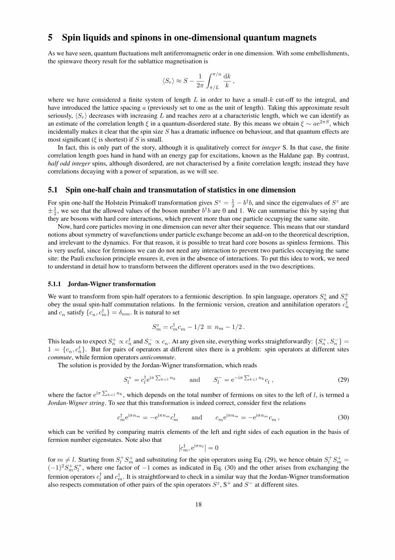
Figure 1: Ground state and excited states of spin one-half XY chain, in Jordan-Wigner fermion description

5.1.4 Excitations

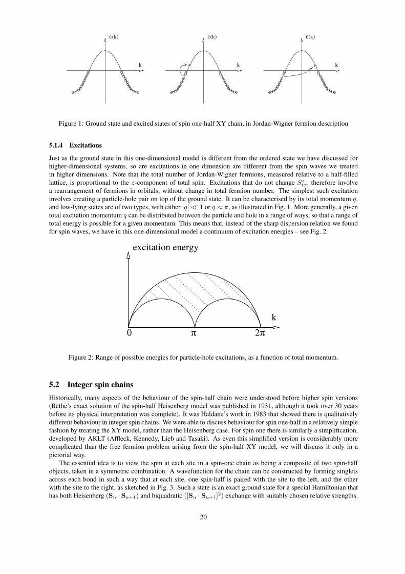
Just as the ground state in this one-dimensional model is different from the ordered state we have discussed forhigher-dimensional systems, so are excitations in one dimension are different from the spin waves we treatedin higher dimensions. Note that the total number of Jordan-Wigner fermions, measured relative to a half-filledlattice, is proportional to the z-component of total spin. Excitations that do not change Sztot therefore involvea rearrangement of fermions in orbitals, without change in total fermion number. The simplest such excitationinvolves creating a particle-hole pair on top of the ground state. It can be characterised by its total momentum q,and low-lying states are of two types, with either |q| 1 or q ≈ π, as illustrated in Fig. 1. More generally, a giventotal excitation momentum q can be distributed between the particle and hole in a range of ways, so that a range oftotal energy is possible for a given momentum. This means that, instead of the sharp dispersion relation we foundfor spin waves, we have in this one-dimensional model a continuum of excitation energies – see Fig. 2.

0

excitation energy

k

π 2π

Figure 2: Range of possible energies for particle-hole excitations, as a function of total momentum.

5.2 Integer spin chainsHistorically, many aspects of the behaviour of the spin-half chain were understood before higher spin versions(Bethe’s exact solution of the spin-half Heisenberg model was published in 1931, although it took over 30 yearsbefore its physical interpretation was complete). It was Haldane’s work in 1983 that showed there is qualitativelydifferent behaviour in integer spin chains. We were able to discuss behaviour for spin one-half in a relatively simplefashion by treating the XY model, rather than the Heisenberg case. For spin one there is similarly a simplification,developed by AKLT (Affleck, Kennedy, Lieb and Tasaki). As even this simplified version is considerably morecomplicated than the free fermion problem arising from the spin-half XY model, we will discuss it only in apictorial way.

The essential idea is to view the spin at each site in a spin-one chain as being a composite of two spin-halfobjects, taken in a symmetric combination. A wavefunction for the chain can be constructed by forming singletsacross each bond in such a way that at each site, one spin-half is paired with the site to the left, and the otherwith the site to the right, as sketched in Fig. 3. Such a state is an exact ground state for a special Hamiltonian thathas both Heisenberg (Sn · Sn+1) and biquadratic ([Sn · Sn+1]2) exchange with suitably chosen relative strengths.

20

To see this, consider – for the wavefunction we have described – possible values of the total spin Stotn,n+1 of two

neighbouring sites, n and n + 1. This total spin is built from four spin-half objects, two of which are in a singletstate. It may therefore take the values 0 or 1, but cannot take the value 2. Such a state is annihilated by theprojection operator P2(Sn + Sn+1) onto Stot

n,n+1 = 2. It is therefore a zero-energy eigenstate of the Hamiltonian

H = J∑n

P2(Sn + Sn+1) (36)

and is a ground state for antiferromagnetic exchange (J > 0), sinceH in this case is a sum of non-negative terms.The projection operator can be written explicitly as

P(L) = |Sn + Sn+1|2(|Sn + Sn+1|2 − 2),

and expansion of this expression yields Heisenberg and biquadratic terms as discussed.

Figure 3: Schematic representation of the AKLT wavefunction. Boxes represent sites of the spin chain, and smallcircles represent spin one-half objects that together form spin one degrees of freedom. Dashed lines indicate thatspin one-half objects from adjacent sites are in singlet states.

It is plausible and true (though the proof takes some work) that this wavefunction has only short range spincorrelations. Note that if we wished to construct a similar state for spin one-half, we would be forced to breaktranslation symmetry, because with just a single spin-half object at each site, we can form singlets only acrossalternate bonds.

6 Weakly interacting Bose gasAs a final example of a system of bosons, we treat excitations in a Bose gas with repulsive interactions betweenparticles, using an approximation that is accurate if interactions are weak. There is good reason for wanting tounderstand this problem in connection with the phenomenon of superfluidity: the flow of Bose liquids withoutviscosity below a transition temperature, as first observed below 2.1 K in liquid 4He. Indeed, an argument due toLandau connects the existence of superfluidity with the form of the excitation spectrum, and we summarise thisargument next.

6.1 Critical superfluid velocity: Landau argumentConsider superfluid of mass M flowing with velocity v, and examine whether friction can arise by generationof excitations, characterised by a wavevector k and an energy ε(k). Suppose production of one such excitationreduces the bulk velocity to v −∆v. From conservation of momentum

Mv = Mv −M∆v + ~k

and from conservation of energy1

2Mv2 =

1

2M |v −∆v|2 + ε(k) .

From these conditions we find at large M that k, v and ε(k) should satisfy ~k · v = ε(k). The left hand sideof this equation can be made arbitrarily close to zero by choosing k to be almost perpendicular to k, but it has amaximum for a given k, obtained by taking k parallel to v. If ~kv < ε(k) for all k then the equality cannot besatisfied and frictional processes of this type are forbidden. This suggests that there should be a critical velocity vcfor superfluid flow, given by vc = mink[ε(k)/k]. For vc to be non-zero, we require a real, interacting Bose liquidto behave quite differently from the non-interacting gas, since without interactions the excitation energies are justthose of individual particles, giving ε(k) = ~2k2/2m for bosons of mass m, and hence vc = 0. Reassuringly, wewill find from the following calculation that interactions have the required effect. For completeness, we should notealso that while a critical velocity of the magnitude these arguments suggest is observed in appropriate experiments,in others there can be additional sources of friction that lead to much lower values of vc.

21

6.2 Model for weakly interacting bosonsThere are two contributions to the Hamiltonian of an interacting Bose gas: the single particle kinetic energy HKE

and the interparticle potential energyHint. We introduce boson creation and annihilation operators for plane wavestates in a box with side L, as in Section 2.3. Then

HKE =∑k

~2k2

2mc†kck .

Short range repulsive interactions of strength parameterised by u are represented in first-quantised form by

Hint =u

2

∑i 6=j

δ(ri − rj) .

Using Eq. (8) this can be written as

Hint =u

2L3

∑kpq

c†kc†pcqck+p−q .

With this, our model is complete, with a HamiltonianH = HKE +Hint.

6.3 Approximate diagonalisation of HamiltonianIn order to apply the techniques set out in Section 2.1 we should approximate H by a quadratic Hamiltonian. Theapproach to take is suggested by recalling the ground state of the non-interacting Bose gas, in which all particlesoccupy the k = 0 state. It is natural to suppose that the occupation of this orbital remains macroscopic for smallu, so that the ground state expectation value 〈c†0c0〉 takes a value N0 which is of the same order as N , the totalnumber of particles. In this case we can approximate the operators c†0 and c0 by the c-number

√N0 and expandH

in decreasing powers of N0. We find

Hint =uN2

0

2L3+uN0

2L3

∑k6=0

[2c†kck + 2c†−kc−k + c†kc

†−k + ckc−k

]+O([N0]0) .

At this stage N0 is unknown, but we can write an operator expression for it, as

N0 = N −∑k 6=0

c†kck .

It is also useful to introduce notation for the average number density ρ = N/L3. Substituting for N0 we obtain

Hint =uρ

2N +

uρ

2

∑k6=0

[c†kck + c†−kc−k + c†kc

†−k + ckc−k

]+O([N0]0)

and henceH =

uρ

2N +

1

2

∑k 6=0

[E(k)

(c†kck + c†−kc−k

)+ uρ

(c†kc†−k + ckc−k

)]+ . . . (37)

with

E(k) =~2k2

2m+ uρ .

At this order we have a quadratic Hamiltonian, which we can diagonalise using the Bogoliubov transformation forbosons set out in Section 2.2.2. From Eq. (11), we find that the dispersion relation for excitations in the Bose gasis

ε(k) =

[(~2k2

2m+ uρ

)2

− (uρ)2

]1/2.

At large k (~2k2/2m uρ), this reduces to the dispersion relation for free particles, but in the opposite limit ithas the form

ε(k) ' ~vk with v =

√uρ

m.

In this way we obtain a critical velocity for superfluid flow, which is proportional to the interaction strength u,illustrating how interactions can lead to behaviour quite different from that in a non-interacting system.

22

7 Landau theory of Fermi liquidsWe now switch our attention to systems of fermions. Our reference point is the free Fermi gas, and in this and latersections we will consider a sequence of modifications to the non-interacting gas that lead to increasingly significantchanges in physical behaviour. The most important physical example of a system of fermions in condensed matterphysics is of course the electron gas in a metal, but it is good to keep in mind as well both the astrophysicalexamples of white dwarf stars and neutron stars, and from terrestrial low-temperature physics, the case of liquid3He. This last system is particularly simple in the sense that it is translationally and rotationally symmetric, therebeing (in contrast to the case of metals) no background lattice of neutralising ions.

Let’s recall some of the distinctive properties of the free Fermi gas at temperatures low compared to the Fermitemperature TF. The heat capacity is linear in temperature, and the Pauli susceptibility is constant, both beingsuppressed by a factor of T/TF compared to their values in a non-degenerate system, as a result of the Pauliexclusion principle. It is remarkable that the same behaviour is measured for electrons in metals and for liquid3He, since in these systems the scale for interaction energies is typically comparable with the Fermi energy andcertainly much larger than the energy scale of the excitations relevant for these physical properties. The objective ofthe Landau theory of Fermi liquids is to understand why interactions have no qualitative effect, and to characterisetheir residual, quantitative consequences.

Before starting our discussion of Fermi liquid theory, it is interesting to consider in a little more detail how wecan characterise the strength of interactions for an electron gas in a uniform neutralising background. This (thejellium model) is a simple situation because it is parameterised by a single quantity: the number density n. Thisquantity sets both the electron spacing (∝ n−1/3) and the Fermi wavevector (∝ n1/3), and we can write the ratioof Coulomb to kinetic energies as

Coulomb energy

kinetic energy∝ (e2n1/3/4πε0)

(~2n2/3/m)=

1

aon1/3

where a0 = 4π~2ε0/me2 is the Bohr radius. The conventionally used parameter is in fact rs, the radius in unitsof a0 of a sphere containing one electron, so that 4πr3s /3 = 1/(na30), and for typical metals rs lies in the range1.8 − 6. Clearly, if Coulomb interactions dominate, rs is large, and if kinetic energy dominates, rs is small. It isat first a surprise to see that interactions are, relatively speaking, weak in the high density limit – the point is thatalthough Coulomb energies grow with increasing density, the kinetic energy grows faster.

We can ask what happens if rs is very large, so that Coulomb repulsion overwhelms the kinetic energy. Thisconstitutes a classical limit, since the zero-point motion is then negligible, and it is straightforward to see thatthe ground state should involve a crystalline arrangement of electrons, to minimise potential energy. This stateis called the Wigner crystal, and the electron gas is known from quantum Monte Carlo simulations to have afirst-order transition from a Fermi liquid phase to the Wigner crystal at a critical value r∗s ∼ 100.

Returning to our main theme of Landau theory, the central assumption is expressed as a statement about thebehaviour of the ground state and long-lived excitations if the interaction strength is varied from zero to its physicalvalue: we suppose that the ground state and excitations evolve smoothly. This means we assume that excitationsin the interacting system can be labelled using the same set of quantum numbers (wavevector and spin) as in theideal Fermi gas. It also means that we assume there are no ground-state phase transitions for interaction strengthsin this range, and so would fail if we were to pass into a Wigner crystal.

7.1 Lifetime of excitationsFor the ideal Fermi gas, states with particle or hole excitations are exact eigenstates, and so have infinite lifetime.This is not the case in the interacting system, and it is important to understand what determines the finite value ofexcitation lifetimes here. A key argument due to Migdal addresses this issue. Consider the scattering rate betweenthe initial and final states sketched in Fig. 4, in which an initially isolated quasiparticle looses energy by scatteringa fermion out of the Fermi sea, leaving a hole behind.

In a calculation of the rate for this process, we should sum over all final states. We can specify the final statein our example via the energies and momenta of the two quasiparticles, since those of the hole are then fixed byconservation of total energy and momentum. Since the energies of the final state quasiparticles cannot exceedthat of the initial particle, and since the quasiparticles must lie outside the Fermi sea, the final state sum is highlyconstrained if the initial quasiparticle energy εk is close to the chemical potential µ, yielding a rate that varies as(εk − µ)2 at zero temperature. This is an important conclusion: because the scattering rate vanishes more rapidlythan the excitation energy εk − µ as the Fermi surface is approached, the energy of low-lying quasiparticles is

23

Figure 4: Left: initial state with a single quasiparticle excitation above a filled Fermi sea. Right: final state withtwo quasiparticles and a quasihole

(in the limit) sharply defined. That is to say, the idea of a sharp Fermi surface is self-consistent, because of therestrictions on scattering processes imposed by Pauli exclusion. Finite temperature sets a lifetime for quasiparticlesat µ proportional to T 2.

7.2 Relation between bare fermions and quasiparticlesThe action on the ground state wavefunction |0〉 for the interacting system of an annihilation operator ckσ for abare fermion with wavevector k and spin σ has an amplitude to generate a state |kσ〉 containing a quasihole withthese quantum numbers if |k| < kF. It also has an amplitude to generate superpositions of many excitations, whichwe denote as |incoherent〉, and we expect the amplitude for such processes to vary smoothly with k. Denoting theamplitude for creation of a quasiparticle by Z1/2, we can summarise these ideas by writing

ckσ|0〉 ∼Z1/2|kσ〉+ |incoherent〉 |k| < kF

|incoherent〉 |k| > kF(38)

Hence the dependence of 〈0|c†kσckσ|0〉 on |k| has a step of size Z at |k| = kF. This is known as the Migdaldiscontinuity and is a demonstration of the existence of a sharp Fermi surface. In the free fermion system Z = 1;the effect of interactions is to decrease Z and to give excitations an effective mass larger than that of the bareparticles.

c><c+

k

Figure 5: Relation between bare fermions and quasiparticles: dependence of occupation number on |k| in theground states of a free Fermi gas (dashed line) and in interacting Fermi liquid (full line).

7.3 Parameterising excitation energiesHaving established the idea that excitations are of the same kind as in a free gas, and have sharply defined energies,it remains to discuss how these energies are influenced by interactions. We specify the state of the system in termsof the occupation number nkσ for quasiparticles with wavevector k and spin σ, and write the energies of thesequasiparticles as εkσ . We separate ground state and excitation contributions by writing nkσ = n0kσ + δnkσ , wheren0kσ = 1 if in the ground state εkσ < µ and is zero otherwise. We expect the energy εkσ of a given quasiparticle todepend on the occupation δnqσ′ of all other excitations: the idea of Landau theory is to represent this dependence

24

using the first terms in a Taylor series, as

εkσ − µ =~2kFm∗

(k − kF) +∑qσ′

f(kσ,qσ′)δnqσ′ . (39)

Here the zeroth order term in δn is assumed linear in the radial deviation k − kF from the Fermi surface, and itsmagnitude is characterised by an effective mass m∗, while the first order terms involve the Landau f -parameters.Note that for physically important excited states, both the relevant values of k − kF and the fraction of non-zeroδnqσ′ are small, so that the two terms retained in Eq. (39) are comparable in magnitude, and parametrically largerthat the neglected higher order terms. At this stage, the approach seems unpromising, because the expansion coef-ficients involve not simply a few fitting parameters but instead an unknown function f(kσ,qσ′). We make thingsmanageable by separating δnqσ′ into spherical harmonics, and recognising that only the lowest two harmonics aregenerated in situations of physical interest. In turn, and assuming a spherically symmetric Fermi surface, only thezeroth and first harmonics of f(kσ,qσ′) are important, and symmetrising also in spin labels we are left with justthree significant Landau parameters. Together with the effective mass they characterise interaction effects.

In more detail, we expect f(kσ,qσ′) to depend (for k and q close to the Fermi surface) only on the angle θbetween these wavevectors, and so (suppressing spin labels) we write

f(kσ,qσ′) =∑l

flPl(cos θ)

with Pl(cos θ) the Legendre polynomials. Similarly, we write

f(k ↑,q ↑) = f(k ↓,q ↓) = f skq + fakq and f(k ↑,q ↓) = f(k ↓,q ↑) = f skq − fakq ,

and finally we use the density of states at the Fermi surface ν(EF) to form dimensionless combinations F =ν(EF)f . The Fermi liquid is then parameterised by

F s0 F a

0 F s1 and m∗

and of these only three are independent, because m∗ and F s1 are related.

7.4 Measuring Landau parametersTo understand the physical significance of these parameters, we should consider the situations in which each ofthem becomes important, by examining different ways of exciting the Fermi liquid.

7.4.1 Heat capacity

Finite temperature generates a distribution of excitations in which there are equal numbers of quasiparticles andquasiholes, so that the density integrated over the radial component of wavevector vanishes:∫

dk δnkσ = 0 .

For this reason interactions affect the heat capacity CV only via the value of effective mass, and

CV =π2

3k2Bν(EF)T =

kFk2B

3~2m∗T .

7.4.2 Compressibility

An increase in density can be represented as an isotropic, spin-independent δnkσ . Let

δn =∑kσ

δnkσ .

The resulting change in the total energy of the system is

δE =~2kFm∗

∑kσ

(k − kF)δnkσ +1

2

∑kσ,qσ′

f(kσ,qσ′) δnkσ δnqσ′

= EoldF δn+

1

2(Enew

F − EoldF )δn+ (f s0 + fa0 )

(δn

2

)2

+ (f s0 − fa0 )

(δn

2

)2

. (40)

25

Now, we also have the relationδn = (Enew

F − EoldF )ν(EF)

and so the change in energy as a result of a volume change is

δE = EoldF δn+

1

2ν(EF)[1 + F s

0 ](δn)2 .

From the energy change we can obtain the compressibility κ, since this quantity, the pressure p, the volume V andthe energy E of a system are related by

p = −∂E∂V

and κ−1 = −V ∂p

∂V

giving

κ =ν(EF)

V· 1

1 + F s0

.

In this result, the first factor is the contribution from the degeneracy pressure of free fermions (note that we havechosen to define ν(EF) for the system as a whole rather then per unit volume, and so it is proportional to V ), whilethe second factor represents the influence of interactions between quasiparticles, which reduce the compressibilityif they are repulsive (F s

0 > 0), as one would expect.

7.4.3 Susceptibility

We can probe the Landau parameter F a0 by considering a measurement of the Pauli susceptibility, since a Zee-

man field generates a spherically symmetric distribution of quasiparticles with opposite signs of δnkσ for spinsorientated parallel or antiparallel to the Zeeman field of strength H .

Letδn↑ ≡

∑k

δnk↑ = −δn↓ ≡∑k

δnk↓ .

Then the magnetisation of the system (writing g for the g-factor of the quasiparticles) is

M =1

2gµB(δn↑ − δn↓) = gµBδn↑

and the change in total energy, consisting of Zeeman, kinetic and interaction terms, is

δE = −gµ0µBHδn↑ +~2kFm∗

∑kσ

(k − kF)δnkσ +1

2

∑kσ,qσ′

f(kσ,qσ′) δnkσδnqσ′

= −gµ0µBHδn↑ +2

ν(EF)(δn↑)

2 +2F a

0

ν(EF)(δn↑)

2 .

Minimising with respect to δn↑ yields the equilibrium value of the magnetisation and the susceptibility

χ =∂M

∂H=µ2Bµ0ν(EF)

1 + F a0

.

In this expression the numerator is the free fermion result modified by replacing bare mass with effective mass,while the denominator includes the influence of interactions between quasiparticles. Note that an attractive inter-action between quasiparticles with the same spin leads to a negative value for F a

0 and an enhancement of χ. In thelimitF a

0 → −1 this produces an instability towards ferromagnetic order.

7.4.4 Galilean invariance

The requirement of Galilean invariance leads to the relation

m∗

m= 1 +

F s1

3

and the derivation of this result is set as Question 1 on Problem Sheet 2.

26

7.4.5 Fermi liquid parameters for 3He

It is interesting to see the measured values of the Landau parameters for 3He, shown in the table below. Notethat the effective mass is greatly enhanced compared to the bare mass, and that this enhancement increases withincreasing density. Note also that the liquid is quite close to a ferromagnetic instability.

m∗/m F s1 F s

0 F a0

Low pressure (0.3 atmospheres) 3.1 6.3 10.8 -0.67High pressure (27 atmospheres) 5.8 14.4 75.6 -0.72

Table 1: Fermi liquid parameters for liquid 3He (from Pines and Nozieres, The Theory of Quantum Liquids).

8 BCS theory of superconductivityWe have seen that the Fermi liquid is stable to weak repulsive interactions, in the sense that excitations retain theircharacter though their energy is modified. Attractive interactions by contrast lead to a qualitative change in theground state and low-temperature properties, no matter how weak they are.

The central idea of BCS theory is that electron-phonon interactions lead to the formation of bound pairs ofelectrons, known as Cooper pairs, which in a sense Bose condense. However, the characteristic size of Cooperpairs – the coherence length – is much larger than their separation, so binding and condensation must be treatedtogether in the theory. The same fact also leads to a simplification: since each Cooper pair interacts with manyothers, mean field theory is a good approximation.

From a historical perspective, it is striking how long the interval was between the experimental discovery ofsuperconductivity, by Onnes in 1911, and the theoretical understanding due to Bardeen, Cooper and Schrieffer in1957: this serves to underline what a revolutionary advance their treatment of a cooperative quantum phenomenonrepresents.

8.1 Electron-phonon interactionsExperiments on the isotope effect showed that phonons are central to superconductivity. In the ideal case, fordifferent isotopes of the same superconductor the energy scales represented by the critical temperature Tc and thecritical field Hc vary with isotope mass like phonon frequencies, as (ionic mass)−1/2. For a pair of electrons thatare close in energy, phonon exchange generates an attractive interaction that beats the obvious screened Coulombrepulsion.

To derive this effective interaction we start from the Hamiltonian H = H0 +H1 written in terms of electronoperators c†k and ck, and phonon operators a†q and aq as

H0 =∑k

ε(k)c†kck + ~ω∑q

a†qaq and H1 =∑kq

(Mc†k+qckaq + h.c.

).

Here ε(k) is the electron dispersion relation and the phonons are represented as Einstein oscillators, all withfrequency ω; the electron-phonon coupling is represented by the matrix element M ; and we have omitted spinlabels, though they will be crucial later.

We wish to focus on the electron system. To this end we eliminate the electron-phonon coupling by means ofa canonical transformation, which we determine perturbatively. We write

H = e−SHeS = H+ [H, S] +1

2[[H, S], S] + . . .

and at leading order we fix S simply by setting

H1 + [H0, S] = 0 , (41)

yielding

H = H0 +1

2[H1, S] ≡ H0 +Hint . (42)

27

To find S explicitly, we take matrix elements of Eq. (41) in eigenstates of H0, which satisfy H0|n〉 = En|n〉. Inthis way we obtain

〈n|S|m〉 =〈n|H1|m〉Em − En

and 〈f |Hint|i〉 =1

2

∑v

〈f |H1|v〉〈v|H1|i〉(

1

Ei − Ev+

1

Ef − Ev

).

From its matrix elements we can read offHint in operator form, as

Hint =1

2

∑pkq

c†p+qcpc†k−qck|M |

2

(1

ε(k)− ε(k− q)− ~ω+

1

ε(p + q)− ε(p)− ~ω

).

8.2 The Cooper problemThis is an attractive interaction for pairs of electrons with |ε(k)−ε(k−q)| < ~ω: that is, for pairs within the Debyeenergy ~ωD of the Fermi surface. It is, however, typically very weak. This leads us to a puzzle: for two particlesmoving in free space in three dimensions, an attractive interaction must exceed a critical strength to produce abound state. So how can a weak attraction generate superconductivity? The Cooper problem takes us one steptowards answering this question: we consider a pair of particles moving not in free space, but above a filled Fermisea, and will find that Pauli exclusion facilitates binding.

Consider the wavefunction for this pair of particles. We want to write a low-energy state, and so we set thecentre-of-mass momentum to zero. To take advantage of a local attractive interaction, we choose the pair to be in aspin-singlet state so that the spatial wavefunction is symmetric. And to respect Pauli exclusion from a filled Fermisea, we require the wavefunction to be built from orbitals outside the Fermi surface. The general form is then

ψ(r1σ1, r2σ2) = (↑1↓2 − ↓1↑2) ·∑|k|>kF

gkeik·(r1−r2)

with gk determined by requiring this to be a solution to the two-particle Schrodinger equation. Writing the pairenergy as E and the pair potential as U(r1 − r2), we have∑

|k|>kF

gk eik·(r1−r2)U(r1 − r2) =∑|k|>kF

(E − 2ε(k))gk eik·(r1−r2) . (43)

To solve this Schrodinger equation, we operate on both sides with1

V

∫dd(r1 − r2) . . . e−iq·(r1−r2)

(where V is the system volume) and introduce the notation∫

ddrU(r)ei(k−q)·r = Ukq . Then Eq. (43) becomes

1

V

∑|k|>kF

gkUkq = (E − 2ε(q))gq .

We can understand the essentials in a simple way by taking

Ukq =

−U if ε(k) and ε(q) are within ~ωD of EF

0 otherwise .(44)

ThenU

V

′∑k

gk = (2ε(q)− E)gq

where∑′

k is a sum over states within ~ωD of EF.

1

V

ε=EF+~ωD∑ε=EF

1

2ε− E=

1

U.

With a constant density of states ρ per unit volume, this yields∫ EF+~ωD

EF

dερ

2ε− E=ρ

2ln

[2(EF + ~ωD)− E

2EF − E

]=

1

U.

There is a bound state for any positive U , and at weak coupling the binding energy is

2EF − E = 2~ωDe−2/ρU .

Strikingly, this form is non-perturbative in ρU .

28

8.3 The BCS wavefunctionGiven a wavefunction for a pair of electrons of the form we have been considering

φ(r1, r2) = (↑1↓2 − ↓1↑2)g(r1 − r2)

we can attempt to write a wavefunction for 2N electrons in which pairs are Bose condensed, of the form

ψ(r1 . . . r2N ) = An=N∏n=1

φ(r2n, r2n+1)

where A denotes antisymmetrisation. It is initially unclear whether Pauli exclusion allows this – whether a non-zero wavefunction survives after the operation of A when N is large. That it does is clearer when we write boththese states in k-space and using operator notation, as

|φ〉 =∑k

gkc†k↑c†−k↓|0〉

and

|ψ〉 =

N∏n=1

(∑kn

gknc†kn↑c

†−kn↓

)|0〉 (45)

since when we expand the product, terms with all kn’s different will survive. The form of the wavefunction inEq. (45) is not very convenient, because the occupation of different orbitals is correlated through the constraintthat exactly 2N electrons are present. The BCS wavefunction relaxes this condition (passing to it is analogous togoing from the cannonical to the grand canonical distributions in statistical mechanics). It has the form

|BCS〉 =∏k

(uk + vkc†k↑c†−k↓)|0〉 . (46)

Here uk is the amplitude for a pair of orbitals to be empty, and vk is the amplitude for them to contain a Cooperpair, so we require |uk|2 + |vk|2 = 1 for normalisation, and

∑k |vk|2 = N in a system containing 2N electrons

on average.In fact, a wavefunction of the form of Eq. (46) can represent a variety of states, depending on the choice of

coefficients vk. A filled Fermi sea simply has vk = 1 for k inside the Fermi surface and vk = 0 outside. Bycontrast, in a state containing many Cooper pairs, we expect vk to vary smoothly between 1 and 0 across a windowof width ~ωD around the Fermi energy. One approach to finding vk is variational, and the subject of Question 2 onProblem Sheet 2. An alternative is a mean field treatment of the Hamiltonian, as described next.

8.4 Mean field theoryUsing the simplified pairing interaction of Eq. (44) the Hamiltonian we are concerned with is

H =∑kσ

εkc†kσckσ − U

′∑kq

c†k↑c†−k↓c−q↓cq↑

where∑′

kq is a sum on states having energies εk, εq within ~ωD of EF.We now wish to treat the interaction term in this Hamiltonian using a mean field approximation, in order to

reduce it to a quadratic form. To this end we let bk = 〈c†k↑c†−k↓〉 and write

c†k↑c†−k↓ = bk +

(c†k↑c

†−k↓ − bk

)with the idea that the sum over k of the term in round brackets is small, and so need be taken only to first order.Then with ξk ≡ εk − µ we have

H− µN =∑kσ

ξkc†kσckσ − U

′∑kq

(bkc−q↓cq↑ + b∗qc

†k↑c†−k↓ − bkb

∗q

)+ fluctuations.

29

Dropping the fluctuation term and setting U∑′

k bk ≡ ∆, this is

H− µN =∑kσ

ξk(c†k↑ck↑ + c†−k↓c−k↓)−′∑k

(∆ c−k↓ck↑ + ∆∗c†k↑c

†−k↓

)+|∆|2

U. (47)

This Hamiltonian is diagonalised by the fermionic Bogoliubov transformation, as described in Section 2.2.1. Set-ting

c†k↑ = ukγ†k0 + v∗kγk1 and c†−k↓ = ukγ

†k1 − v

∗kγk0

we require |uk|2 + |vk|2 = 1 to preserve anticommutation relations, and 2ξkukvk +∆v2k−∆∗u2k = 0 to eliminatenumber-changing terms from the transformed Hamiltonian. Writing ∆ = eiφ|∆| these conditions are met by

uk = eiφ/2 cos θk, vk = e−iφ/2 sin θk and cot 2θk =ξk|∆|

.

Note that for ξk |∆|, θk → 0 and so c†k↑ ∼ γ†k0 and c†−k↓ ∼ γ

†k1. Conversely, for ξk −|∆|, θk → π/2 and so

c†k↑ ∼ γk1 and c†−k↓ ∼ γk0. The γ-particles thus interpolate between electrons and holes, and at the Fermi energy,where ξk = 0 and θk = π/4, have equal electron and hole content.

After Bogoliubov transformation, the Hamiltonian is

H− µN =∑kσ

√ξ2k + |∆|2

(γ†k0γk0 + γ†k1γk1

)+∑k

(ξk −

√ξ2k + |∆|2

)+|∆|2

U. (48)

Crucially, the value of |∆| must be determined self-consistently. We have

|∆| = U

′∑k

|〈c†k↑c†−k↓〉| = U

′∑k

ukv∗k

(1− 〈γ†k0γk0〉 − 〈γ

†k1γk1〉

). (49)

At zero temperature 〈γ†k0γk0〉 = 〈γ†k1γk1〉 = 0. Then with a constant density of states ρ we have

1 =ρU

2

∫ −~ωD

−~ωD

dξ√ξ2 + |∆|2

.

For ~ωD |∆| this gives 1 ≈ ρU ln(~ωD/|∆|) and we find

|∆| = 2~ωDe−1/ρU

as we did for the pair binding energy in the Cooper problem.At finite temperature 〈γ†k0γk0〉 and 〈γ†k1γk1〉 are determined from the quasiparticle energies using the Fermi

distribution, and the gap |∆| decreases as temperature decreases. Above a critical temperature Tc, the only solutionto the self-consistency condition is ∆ = 0. Moreover, since at weak coupling ρU is the only parameter, the energyscales set by the zero-temperature gap and the thermal energy at the critical point have a universal relationship thatserves as a test of the theory:

2|∆(T=0)|kBTc

= 3.53 .

The form of the quasiparticle density of states, probed by tunneling spectroscopy, provides another experimentaltest of these ideas.

9 The Mott transition and the Hubbard modelWe now consider the combined consequences for electrons in a solid of electron-electron interactions and thebackground ionic lattice. Our most important conclusion will be that a new type of insulator is possible, in additionto the band insulator familiar from single-particle theory. Specifically, while in a solid without electron-electroninteractions we have a insulator (in the absence of band overlap) when the number of electrons per unit cell is even,we shall see that strong correlations in a half-filled band with an odd number of electrons per unit cell can generatea new state known as a Mott insulator.

30

9.1 The Hubbard modelIn the standard theoretical description of this phenomenon we use a tight-binding model

H0 = −t∑〈rr′〉σ

c†r σcr′σ

and add only intra-site Coulomb interactions, of the form

HI = U∑r

nr↑nr↓ (50)

where nrσ = c†rσcrσ . The Hubbard model Hamiltonian is then

H = H0 +HI . (51)

We would like to understand its phase diagram as a function of U/t, band-filling and temperature. At small Uand above one dimension we expect Fermi liquid behaviour, from the same arguments that led to Landau theory,but at large U with one electron per site we find an insulator, by the following argument. In this regime there is aset of low energy states in which every site is singly occupied. Charge motion requires generation of empty anddoubly occupied sites, and so is energetically prohibited.

9.1.1 Relation to the Heisenberg model

At large U and half filling, the set of low-lying states has a degeneracy of 2N in a system of N lattice sites, arisingfrom the choices of spin orientation at each site, in the limit t/U → 0. Virtual hopping lifts this degeneracyand gives rise to Heisenberg exchange, as follows. Consider a pair of sites and treat the effects of H0 usingperturbation theory. We can label eigenstates of the unperturbed Hamiltonian HI as | ↑, ↑〉, | ↑, ↓〉 and so on. Theleading contributions to their energies are at second order, and are

δE↑,↑ = 0 and δE↑,↓ = −2t2

Ufrom

|〈↑, ↓ |H0| ↑↓, 0〉|2

E↑,↓ − E↑↓,0and similar.

Compare these with the energies of eigenstates of the spin HamiltonianH = Js1 ·s2, which are Esinglet = −3J/4and Etriplet = J/4, and hence split by J . Noting that | ↑, ↑〉 is a triplet state, while | ↑, ↓〉 = 2−1/2[|singlet〉 +|triplet〉], we recognise that the Hubbard model with a half-filled band and large U reduces at low energy to theantiferromagnetic Heisenberg model. We read off the exchange strength, as

J =4t2

U.

9.2 Mott transition

2dt

E

Density of states

U

µ µ

E

Density of states

Figure 6: Spectral function expected for Hubbard model at half filling, showing upper and lower Hubbard bands:(left) in the insulating phase at large U/t; (right) in the metallic phase at small U/t.

It is an important and heavily-studied problem to understand behviour at half-filling as U/t is reduced. Wewill restrict ourselves to some cartoons. At large U added electrons each cost energy U as they necessarily hop

31

between doubly occupied sites with an associated kinetic energy scale t. Holes are also mobile with kinetic energyt, but their creation does not involve the energy penalty U . We therefore expect a spectral density at large U asshown in Fig. 6: at half-filling a fully occupied hole band and an empty electron band, both of widthO(t), are splitby U and sit symmetrically in energy either side of the chemical potential. Reducing the Hubbard repulsion, thesebands overlap at a critical value Uc ∼ 2dt and one expects a phase transition to metallic behaviour. As we increaseU starting from the metallic side, we expect the Migdal discontinuity Z (see Fig. 5) to decrease, reaching zero atthe transition. Indeed, deep in the Mott insulator, it is easy to see that there is no sign of the Fermi surface, sincethe ground state occupation is simply

〈c†kck〉 =1

N

∑rr′

〈c†rcr′〉ei(r′−r)·k =

1

2

for all k, independent of wavevector.

10 The Kondo effectWe now consider the consequences of large Hubbard repulsion acting just at one site of a lattice, to represent animpurity atom at that point. It is a surprise to find that this situation, apparently so close to a free-particle one,should generate a subtle many-body problem, involving what is known as the Kondo effect.

Experimentally, the resistance of many metals and alloys decreases with decreasing temperature as inelasticscattering processes are suppressed. Alloys containing dilute magnetic moments, such as a low concentration ofMn or Fe in Cu, are an exception: they show a resistivity minimum as a function of temperature and below it anincrease in resistivity with decreasing temperature. An explanation of the minimum was given by Kondo in 1964,but it took a decade before the nature of the ground state was properly understood, and it was only in 1980 that amodel for the phenomenon was solved exactly.

10.1 ModelThe Kondo Hamiltonian describes a conduction band of independent electrons interacting via exchange with asingle local moment on the impurity site, chosen to lie at the origin. Then

H =∑kσ

εkc†kσckσ +H1 with H1 = J S · s(0) . (52)

Here S represents the local moment and s(0) is the spin density of the conduction electrons at the impurity site.We can write the exchange interaction as

J S · s(0) = J

[Szsz(0) +

1

2

(S+s−(0) + S−s+(0)

)]=

J

V

∑kq

[Sz(c†k↑cq↑ − c

†k↓cq↓

)+(S+c†k↓cq↑ + S−c†k↑cq↓

)](53)

10.2 Scattering amplitudeThe impurity spin mediates interactions between the conduction electrons, since the state of the impurity spin ata given time depends on previous scattering events. To see the consequences, we will calculate the scatteringamplitude for an electron, taking as our example an initial state ki ↑ and a final state kf ↑, and working to secondorder in J , which will give the scattering rate to O(J3).

At first order, the amplitude (left in the form of an operator on the impurity spin) is

〈kf ↑ |H1|ki ↑〉 =JSz

V.

From this we can find the scattering rate atO(J2), which is independent of temperature in the absence of a Zeemanfield.

At second order we require ∑v

〈kf ↑ |H1|v〉1

ε− εv〈v|H1|ki ↑〉

32

where ε = εki = εkfis the energy of the initial and final states, and |v〉 is an intermediate state with energy εv .

The interesting contributions arise from |v〉 in which the impurity spin is flipped. These involve

S+c†q↓cki↑1

ε− [ε+ εkf− εq]

S−c†kf↑cq↓ and S−c†kf↑cq↓1

ε− [ε− εki+ εq]

S+c†q↓cki↑ .

Now take a thermal average over scattering processes into the intermediate state, by making the replacements

c†q↓cq↓ → 〈c†q↓cq↓〉 = f(εq) and cq↓c

†q↓ → 〈cq↓c

†q↓〉 = 1− f(εq)

where f(ε) = [e−β(ε−µ) + 1]−1 is the Fermi function. Combining terms (and noting a negative sign arising fromexchanging the order of cki↑ and c†kf↑ in the first term), we then have contributions to the amplitude of

J2

V

∑q

1

εk − εq

S+S−f(εq) + S−S+[1− f(εq)]

= S−S+ J2

V

∑q

1

εk − εq+ [S+, S−]

J2

V

∑q

f(εq)

εk − εq. (54)

The factor [εk − εq]−1 in the sums on the right hand side is divergent at the energy εk of the particle whosescattering amplitude we are calculating, which in the case of most interest is the Fermi energy. For the first sum,this divergence is not important, since contributions from above and below the Fermi energy cancel to leave a finiteresult. But in the second term the Fermi function limits this cancellation and we obtain

[S+, S−]1

V

∑q

f(εq)

εk − εq= 2Szρ ln(D/kBT ) ,

where D is the energy width of the conduction band, which sets a lower limit on the sum, and ρ is the density ofstates in energy. To calculate the scattering rate we square the amplitude: combining our first and second orderresults, we find a result proportional to

J2 + 4J3ρ ln(D/kBT )

which grows with decreasing temperature. Combined with a phonon contribution to the electron scattering rate,this yields a minimum in the resistance as a function of temperature for alloys with magnetic impurities, which isthe essence of the Kondo effect. The temperature scale at which the logarithmic term becomes important is theKondo temperature TK = De−1/2ρJ . For the physically relevant regime in which Jρ is small, TK D.

At temperatures T TK perturbation theory is not helpful. Instead we would like to understand the groundstate for the coupled system consisting of the impurity spin and the Fermi gas. It turns out that this is just thesame as one would guess by considering the strong coupling limit in which Jρ is large: for antiferromagnetic Jthe impurity spin binds a conduction electron into a singlet state. This is characterised by a Pauli susceptibility(as distinct from the Curie susceptibility of a free impurity spin) and by a finite scattering rate for the remainingconduction electrons from the bound complex.

11 Disordered conductors and Anderson localisationThe theory of electron energy bands in solids gives an understanding of how the different properties of conductorsand insulators arise. This picture, based on single-particle quantum mechanics for electrons in a periodic lattice,can fail when interactions are strong, as we have seen in our discussion of Mott insulators. It can also fail ifdisorder, in the form of deviations from a perfectly periodic lattice potential, is sufficiently large. This type ofinsulator is known as an Anderson insulator.

11.1 Anderson localisationConsider electrons in impure or amorphous metals or doped semiconductors as examples of waves in a disorderedmedium. At weak disorder the main consequence of impurities is a finite elastic mean free path `el for electrons.This terminology emphasises a scattering description, but we can also discuss eigenstates in a large, finite system.At weak disorder an individual eigenstate is a superposition of waves with similar energies. Locally this super-position generates a plane wave, but the amplitude and phase of the wave vary on the scale of `el, which in thisregime is large compared to the other relevant lengthscale, the Fermi wavelength λF.

33

The question arises: what happens if disorder is increased until what is known as the Ioffe-Regel limit, `el ∼λF? At strong disorder (and also at weak disorder, in low dimensional systems), the nature of eigenfunctions in factchanges. In place of extended states, with the probability density of each individual state spread through the entiresample, eigenstates are spatially localised, with each electron trapped in its own localisation volume, of linear sizeξ.

It is useful to compare this situation with other, more familiar eigenstate problems. An individual localisedstate is similar to the impurity state bound to a donor or acceptor in a semiconductor, in the sense that both statesare spatially localised. There is, however an important difference in that the donor or acceptor levels are isolated inenergy from other states, since they lie in the band gap of the semiconductor. By contrast in an Anderson insulator,we have a band of localised states, and some are very close in energy though far apart in space.

11.2 Stability of localised statesAn immediate question is whether such a situation can be stable. In general, states that are close in energy areeasily mixed by a perturbation, and if we mix two localised states with widely separated centres, the resultingsuperpositions are much less localised than the initial states. Suppose that the mixing is due to a small changeδV in the potential felt by electrons, arising for example because of a change in the disorder realisation. Theconsequent change δψi in an eigenfunction with energy Ei is at first order in perturbation theory

δψi =∑k

〈ψk|δV |ψi〉Ei − Ek

ψk

and the fact that states nearby in energy are easily mixed is represented here by the possibility of small denomina-tors Ei−Ek. More specifically, with density of states ρ per unit energy and volume, the smallest value of Ei−Ekarising from states k that have their localisation centres within a distance r of the state i is (ρrd)−1. We are savedfrom divergent contributions to the sum at large r because for localised states the matrix element in the numeratorfall off even faster: we expect

〈ψk|δV |ψi〉 ∼ e−r/ξ .

In this way we see that the idea of a dense set of localised states is at least self-consistent.

11.3 Mobility edgeThe strength of disorder is characterised by the amplitude of fluctuations in the potential felt by electrons, whichshould be compared with their kinetic energy to obtain a dimensionless measure. For that reason, in a given systemelectrons at low energy are in strong relative disorder, and those are high energy are at weak relative disorder. Inconsequence, if there is a transition in the nature of eigenstates as a function of disorder strength, there will be adivision in the properties of states as a function of energy, with localised states at low energy and extended statesat high energy. The dividing energy is called the mobility edge. Localised states can be characterised by theirlocalisation length ξ and extended states by the value of the conductivity σ, and we expect the behaviour shown inFig. 7.

11.4 Scaling theoryThe change in behaviour from extended to localised states as a function of energy or disorder is (in a non-thermodynamic sense) a phase transition. The field-theoretic description (in terms of a non-linear sigma model)is quite involved, but there is also a simple phenomenological approach based on scaling ideas, known as one-parameter scaling theory. It has some useful predictive power and also offers a good setting for thinking aboutrenormalisation group ideas.

In general, scaling approaches involve asking how physical properties of a system change with lengthscale.Here we focus on the conductance G(L) of a (hyper)-cubic sample in d-dimensions, of linear size L. We measurethis in units of the conductance quantum, e2/h, writing

g(L) =G(L)

e2/h.

Now suppose we combine 2d such hypercubes to make a larger hypercube, of size 2L. The hypothesis of scalingtheory is that the conductance of this final cube depends only on the conductances of the initial cubes, and not on

34

Mobility edge

E

σ

ξ

ρ

Figure 7: Behaviour in a disordered system of the density of states ρ, localisation length ξ and conductivty σ as afunction of energy E. States are localised below a critical energy – the mobility edge – and extended above it.

other characteristics. That is to say, for example, we would get the same result for the final cube by combiningvery small, highly disordered initial cubes or larger, weakly disordered initial cubes, provided the initial value ofG were the same in both cases. We express this idea by writing

∂ ln g

∂ lnL= β(g) .

The beta function β(g) encapsulates the nature of the transition. Of course, we know only a little about it. We can,however, be confident that it is a continuous, smooth function, since it represents behaviour in a finite sample. Wecan also pin down its asymptotics quite easily, as follows.

Consider first the weak disorder limit. Here we expect metallic behaviour characterised by a fixed value forthe conductivity σ of the material, so that G(L) = σLd−2. Hence β(g) = d − 2 at large g. Next considerstrong disorder and assume states are localised. In this regime we anticipate G ∝ exp(−L/ξ) which leads toβ(g) = ln(g) + constant. Connecting the two limits with a smooth monotonic curve yields the result shown inFig. 8.

(g)

d=2

d=1

d=3

ln(g)

β

Figure 8: Dependence of the beta-function β(g) for Anderson localisation on dimensionless conductance g, shownas a function of ln(g) in dimensions d = 1, 2 and 3. For d = 3 the position ln(gc) of the critical point at which thebeta function has a zero is marked by the vertical dashed line.

We should now examine the consequences the follow from the assumptions we have made. It is useful toseparate various cases.

35

d = 1 and d = 2. In this case we always have β(g) < 0. As a result, g(L) decreases with increasing L,eventually exponentially. That is to say, states are localised in d = 1 and d = 2 by arbitrarily weak disorder.

d > 2 and g < gc. In this regime we again have β(g) < 0. With increasing L we find that β(g) becomesincreasingly negative, and states are localised.

d > 2 and g > gc. In this case g increases with L and at large L reaches values for which β(g) = d− 2, sothat we have an Ohmic metal with g(L) ∝ Ld−2

d > 2 and g = gc. In the case of a system with critical disorder the conductance is independent of systemsize – an example of scale-independence at a critical point.

12 The integer and fractional quantum Hall effectsWe now switch to a discussion of the consequences of disorder and of electron-electron interactions for a two-dimensional electron gas in a strong magnetic field. This is a situation in which departures from the behaviourof an ideal, non-interacting Fermi gas without impurity scattering are essentially guaranteed, because the singleparticle eigenstates of the ideal problem are macroscopically degenerate. Our interest is in the ways this degeneracymay be lifted.

The experimental systems are electrons (or holes) in quasi two-dimensional semiconductor structures - eithermetal-oxide-semiconductor field effect transistors fabricated on silicon, or heterostructures or quantum wells fab-ricated from GaAs and AlxGa1−xAs. Carrier motion in the third dimension is frozen out quantum mechanicallywhen temperature and electron density are both small enough that only the lowest sub-band is occupied.

The quantum mechanics of electron motion in a magnetic field with flux density B is characterised by twoscales. One – the cyclotron frequency ωc = eB/m∗ – is classical and material-dependent through the value ofthe effective mass. The other – the magnetic length lB = (~/eB)1/2 – is quantum-mechanical and material-independent. The energy spectrum for the single-particle problem without disorder consists of a sequence ofLandau levels, with energies

E =

(n+

1

2

)~ωc ±

1

2g∗µBB .

For electrons in free space the orbital splitting ~ωc is almost degenerate with the spin splitting gµBB, but forelectrons in a semiconductor ~ωc is typically much larger than g∗µBB, since effective masses are typically smallerthan the bare mass, and the effective g-factor g∗ is also reduced because of spin-orbit interactions. The numberof states within each spin-split Landau level is given simply by the number Nφ of magnetic flux quanta passingthrough the area of the system. Comparing this degeneracy with the number Ne of electrons we obtain the mostimportant parameter characterising the system: the Landau level filling factor ν = Ne/Nφ. For an electron gaswith number density n we have the relation

n = νeB

h.

As a prelude to a discussion of experimental observations, it is useful to recall the Hall effect in an idealsystem, as shown in Fig. 9. Taking the electrons to have a drift velocity vDrift, the current is I = evDriftnw =e2

h νBvDriftw while the Hall voltage is VH = BvDriftw. Combining these two expressions, the Hall conductivityis σxy ≡ I/VH = e2ν/h.

Experimentally, studying the resistivity tensor ρ as a function of magnetic field strength or electron density,around certain filling factors accurately quantised plateaus are observed in ρxy accompanied by vanishing ρxx.Under these conditions the forms of the resistivity tensor ρ and the conductivity tensor σ are

ρ =h

νe2

(0 1−1 0

)and σ ≡ ρ−1 =

νe2

h

(0 −11 0

).

It is striking at first sight that both ρxx and σxx should vanish: the important point is simply that the current densityis perpendicular to the field, and so dissipation vanishes.

This observed behaviour is quite different from that expected for a clean, single-particle system. Instead ofa Hall conductance proportional to filling factor and vanishing dissipative conductance, plateaus are seen in Hallconductance as a function of filling factor and the dissipative conductance, though small in quantum Hall plateaus,has peaks at the transtions between plateaus.

36

H

B

I w

V

Figure 9: Schematic view of the Hall effect in a two-dimesional system: current flow I in the presence of amagnetic field B generates a Hall voltage VH in a sample of width w.

12.1 Integer quantum Hall effectThe existence of plateaus around integer values of ν can be understood if we suppose that disorder affects the statesin a Landau level as illustrated in Fig. 10, with Anderson localised states in both the low and high energy tails of thedisorder-broadened Landau level, and a divergence in the localisation length near the Landau level centre. Then, ifthe Fermi energy lies between the centres of two Landau levels, changes in filling factor do not alter the number ofextended, current-carrying states that are occupied, and so the Hall conductance is unchanged. In this situation theabsence of dissipation can also be understood, since dissipative processes require excitation of an electron initiallyin a current-carrying state to an empty final state. As the occupied, current carrying states are buried a finite energybelow the Fermi energy, such processes are suppressed at low temperature by an activation factor.

extended

localised

E

ρ,ξ ξ

ρ

Figure 10: Disorder-broadened Landau level, showing localisation physics necessary to explain the integer quan-tum Hall effect. The dependence of the density of states ρ and the localisation length ξ is given as a function ofenergy E. Almost all states in the Landau level are localised, but the localisation length diverges at a critical pointnear the centre of the Landau level.

12.1.1 Exactness of quantisation

While we can understand the existence of Hall plateaus if we accept this picture for the influence of disorder onelectron eigenstates, the precise quantisation of Hall conductance immediately becomes a surprise, since one mighthave expected the reduction in the number of extended states to be accompanied by a reduced value for the Hallconductance. Clearly, the remaining extended states must carry an extra current in a way that exactly compensatesfor their reduced number.

One way to understand the exactness of quantisation is from the thought-experiment illustrated in Fig 11. Weconsider a quantum Hall sample in the form of an annulus. In addition to the magnetic field responsible for thequantum Hall effect, which pierces the surface of the annulus, we introduce a second magnetic flux Φ, threading

37

through the hole at the centre of the annulus. Allowing this flux to vary as a function of time, we generate a voltageV around the circumference of the quantum Hall sample. From Faraday’s law, we have

V = −dΦ

dt.

Within a Hall plateau, this produces a current flow

I = σxyV

in the perpendicular direction, which is radial. Integrating the rates of flux change and current flow over time, agiven flux difference ∆Φ corresponds to the transport of a certain charge Q between the inner and outer edges ofthe annulus. Now, we expect that a change in Φ of one flux quantum (h/e) will return the interior of the quantumHall system to its initial state, implying that an integer number of electrons have then been transported across theannulus. We have

integer× e = Q = σxy ·∆Φ = σxyh

e

and hence

σxy = integer× e2

h.

I

Φ

V

Figure 11: Geometry considered in Laughlin argument for exactness of quantisation of Hall conductance

12.1.2 Localisation

energy tail

+

+

−

−

extended, percolating trajectory

localised, high

energy tail

localised, low

Figure 12: Trajectories for cyclotron motion guiding centres of charged particles in a smooth random potentialand perpendicular magnetic field, showing how an extended trajectory arises near the Landau level centre, andlocalised trajectories in the low and high energy tails. Lines represent equipotentials and + and − signs denotemaxima and minima of the potential.

38

Anderson localisation in the context of the quantum Hall effect can be understood to some extent by appealingto a semiclassical limit, in which the magnetic length is much smaller than the correlation length for the randompotential that represents disorder. In this case there is a separation of scales: considered classically, the electronmotion can be separated into a fast cyclotron orbit around an instantaneous guiding centre, and slow drift of thisguiding centre. The drift is in a direction perpendicular to the local electric field and therefore along equipotentials.Quantisation of the rapid cyclotron motion generates Landau levels, and the energies of electrons within eachLandau level are displaced by the energy of the equipotential along which they move. In this picture, questionsabout localisation reduce to ones about the nature of equipotential lines. As illustrated in Fig. 12, we expect theseto exhibit a percolation transition, separating low energy closed trajectories which orbit minima in the potentialfrom high energy trajectories which orbit maxima in the potential.

An obvious question now is how this picture of a delocalisation transition in quantum Hall systems can berelated to the scaling theory described in Section 11.4. In particular, whereas we had concluded earlier that ina two-dimensional system states should be localised, we now see that this is not always the case. A scalingflow diagram that reconciles the earlier discussion with behaviour in quantum Hall systems is shown in Fig. 13.Crucially, in a magnetic field we consider the scaling flow of the two independent components of the conductivitytensor. The scaling flow diagram shows how these evolve as a system is probed on increasing lengthscales –experimentally, by lowering temperature to increase the inelastic scattering length that cuts off phase coherentlocalisation effects. The scaling flow diagram is periodic in the Hall conductance, measured here in units of thequantum e2/h and contains fixed points of two types. Stable fixed points at (σxx, σxy) = (0, n) with n integerdescribe the insulating state in zero magnetic field and also the system in quantum Hall plateaus. Unstable fixedpoints located at (σxx, σxy) = (σ∗, n+1/2) describe the delocalisation transitions that separate different quantumHall plateaus.

∗

σ

σ

xy

xx

0 1 2

σ

Figure 13: Scaling flow diagram for quantum Hall plateau transitions.

12.2 Fractional quantum Hall effectIn sufficiently high mobility samples, quantum Hall plateaus are observed with certain simple fractional valuesof the Hall conductance, in addition to the integer plateaus we have discussed. Specifically, one finds σxy =(p/q) · (e2/h), with p and q integer, and q (in nearly all cases) odd. The fact that this is observed in samples withlow disorder suggests it is interactions that lift the degeneracy of the partially filled Landau level, forming specialcorrelated ground states at certain filling factors. And the fact that σxx → 0 at low temperature (with an activatedtemperature dependence) suggests there is a gap for excitations from these correlated ground states. Moreover,Laughlin’s argument for quantisation of Hall conductance suggests that excitations have fractional charge, sincewe argued that σxy × (h/e) should be equal to the charge transported across an annular system when one fluxquantum is inserted. Assuming this charge consists of an integer number of quasiparticles, each of charge e∗, wehave (p/q)e = integer× e∗.

39

12.2.1 Single particle in a magnetic field

As a first step, it is useful to summarise some results for the quantum mechanics of a particle in a magnetic field.We take charge −e and magnetic field (0, 0,−B), with e and B positive. The Hamiltonian is

H =1

2m∗(π2x + π2

y) with ~π = −i~~∇+ e ~A

and

[πx, πy] = −i~e(∂xAy − ∂yAx) =i~2

l2B.

We define raising and lowering operators

a† =lB√2~

(πx − iπy) and a =lB√2~

(πx + iπy) with [a, a†] = 1

so thatH = ~ωc(a

†a+ 1/2) .

Now, it is convenient to combine coordinates into a complex number, by writing z = x + iy and z = x − iy. Wealso use the notation

∂z =1

2(∂x − i∂y) and ∂z =

1

2(∂x + i∂y) ,

which is set up so that, for example,

∂zz = ∂zz = 1 and ∂zz = ∂zz = 0 .

Choosing units in which lB = 1 and taking the gauge ~A = (B/2)(y,−x, 0) we then have

a = − i√2

(2∂z +1

2z) .

Ground state wavefunctions ψm satisfy aψm = 0, and a complete set is

ψm ∝ zme−|z|2/4

withm = 0, 1, 2 . . .. The proabability density of themth state is a ring with (after restoring units) radius (2m)1/2lBand width lB.

12.2.2 Two particle problem

Unsymmetrised two-particle basis states from the lowest Landau level have the form

ψ(z1, z2) ∝ zl1zm2 e−(|z1|2+|z2|2)/4

with l,m non-negative integers. We will consider combinations of these that are eigenfunctions of relative andcentre-of-mass angular momentum. They have the form

ψ(z1, z2) ∝ (z1 − z2)l(z1 + z2)me−(|z1|2+|z2|2)/4 .

The value of l completely determines the typical particle separation in the state and fixes the energy given a formfor the interaction potential. For this reason, and in contrast to a two-particle problem without restriction to a singleLandau level, the pair is incompressible. By this we mean that the two-particle system cannot respond smoothlyto an external potential that for example squeezes the particles together. Instead, with increasing external potentialwe expect a sequence of level crossings at which the ground state value of l changes: at each crossing there is ajump in the separation of the particles, but between jumps their separation is independent of the external potential.

Note that l is required by the statistics of the particles to be odd for fermions, or even for bosons.

40

12.2.3 Laughlin wavefunction

With this discussion of the two-particle problem as orientation, we can consider the many-particle wavefunctionproposed by Laughlin

ψ(z1 . . . zN ) =∏i<j

(zi − zj)qe−14

∑k |zk|

2

.

As motivation for this form, one can begin with the intention of writing a variational state containing so-calledJastrow factors of the form f(zi − zj). Trial wavefunctions of this form have been used successfully, for example,in the theory of superfluid 4He, where an appropriate choice for the function making up the Jastrow factor enablesone to build two-particle correlations into the wavefunction that minimise the energy of the system. Restriction tothe lowest Landau dramatically constrains this choice of function, to the discrete set (zi − zj)q , with q a positiveinteger, which must be odd for fermions or even for bosons. The value q = 1 describes a full Landau level.Higher values ensure that the probability density falls faster to zero as a pair of particles approach each other(as |zi − zj |2q) than in a generic antisymmetric state, and for this reason are good variational choices when theinterparticle interaction is repulsive. In fact, this wavefunction is an exact ground state for a certain interparticlepotential (a generalised delta function), and is known from numerical studies on systems containing a small numberof particles to have very high overlap with exact ground states for systems with Coulomb interactions.

In many-particle quantum mechanics, knowledge of the wavefunction is not all, since extraction of physicalinformation from this function of many coordinates constitutes a problem as hard as the one in classical statisticalmechanics of calculating physical averages from a Boltzmann factor that is a function of the coordinates of allparticles in a system.

The simplest question we might ask is what filling factor is represented by the Laughlin wavefunction. Ex-panding, we see that the largest power of each coordinate is zq(N−1)i . Recalling that the single-particle wavefuctionz e−|z|

2/4 has its probability density concentrated on a ring of radius ∝ m1/2, we see that in the Laughlin state Nparticles fill the area that would be occupied by qN + 1 − q particles if the Landau level were completely filled.Hence we see for large N that

ν =1

q.

As a next and much harder step we would like to understand correlations in the Laughlin state. A goodapproach to this problem is to use what is called the plasma analogy: we think of the probability density arisingfrom this wavefunction as if it were the Boltzmann weight for a problem in classical statistical mechanics. We canread off the Hamiltonian for this classical problem, which turns out to be a Coulomb gas, or plasma. If we havegood physical intuition for the statistical mechanics of plasmas, we can apply this to draw conclusions about theLaughlin state.

Some details are as follows. We define a fictitious inverse temperature β and classical HamiltonianHcl via

|ψ(z1 . . . zn)|2 = e−βHcl .

This yields

Hcl =1

2β

∑k

|zk|2 −2q

β

∑i<j

ln |zi − zj | .

To interpret this form we should recall electrostatics in two dimensions: a point charge Q at the origin gives rise atradius r to an electric field

E(r) =Q

2πε0rand a potential V (r) = − Q

2πε0ln r .

It is convenient to set the (arbitrary) inverse temperature to β = 4πε0/q. Then the two-particle term inHcl becomes

− q2

2πε0

∑i<j

ln |zi − zj | ,

which represents the electrostatic interaction of particles with charge q. The single particle term is

q

8πε0

∑k

|zk|2 .

41

It would arise for particles of charge q moving in an electrostatic potential |z|2/(8πε0). We can view this potentialas arising from a background charge distribution, and find the density of this charges using Poisson’s equation. Weobtain a density

−ε0∇2 1

8πε0|z|2 = − 1

2π.

As a first conclusion from this picture, we can recover the value of the Landau level filling factor ν. The plasmaconsisting of N particles each with charge q will arrange itself so as to cancel on average the background charge,by adopting a mean number density of 1/(2πq). Since this is the number density of electrons in the Laughlinstate (remember that we set lB to unity), and since its value is 1/q of the value for the filled Landau level, weobtain again ν = q−1. Going futher, we can use the plasma analogy to discuss electron-electron correlations in theLaughlin wavefunction. In fact, the plasma is known to be fluid for q . 70 and crystalline for q & 70, and so wesee that the Laughlin wavefunction represents a liquid state for the important values q = 3, 5 . . ..

One can also use Laughlin’s approach to write down a wavefunction including a hole, and use the plasmaanalogy to examine its properties. We have

ψhole(z1 . . . zN ) =∏l

(zl − ξ)× ψLaughlin(z1 . . . zN ) .

The extra factor has the effect of excluding electrons from the vicinity of the point ξ where the hole is located.Within the plasma analogy we find

Hcl → Hcl −q

2πε0

∑l

ln |zl − ξ| .

Thus the hole translates to a particle of unit charge in the plasma, located at ξ and interacting with other particles, ofcharge q at zl. Since plasmas screen, this will induce a compensatiing reduction in the plasma density around it, butsince the plasma particles have charge q, a deficit of only 1/q plasma particles is sufficient for exact compensation.Back in the language of electrons, a deficit of 1/q of an electron means that the hole has charge 1/q. This is aspectacular instance of fractionalisation, and fractional charge has been observed reasonably directly in shot noisemeasurements on current carried by fractional quantum Hall quasiparticles.

42