galactic and planetary dynamics - rudolf peierls centre ... · 3 galactic and planetary dynamics...
TRANSCRIPT
Galactic and planetary dynamics
These are incomplete notes for the MMathPhys course on “galactic and planetary dynamics”. The mostup-to-date version is available from http://www-thphys.physics.ox.ac.uk/people/JohnMagorrian/cm21.
Course outline: Review of Hamiltonian mechanics. Orbit integration. Classification of orbits and integra-bility. Construction of angle–action variables. Hamiltonian perturbation theory. Simple examples of itsapplication to the evolution of planetary and stellar orbits. Methods for constructing equilibrium galaxymodels. Applications. Fundamentals of N -body simulation. Dynamical evolution of isolated galaxies. In-teractions with companions.
1 Review of Hamiltonian mechanics
Recall that the arena for Lagrangian mechanics is configuration space, whose dimension is equal to thenumber of degrees of freedom of the system. The Lagrangian L(q, q, t) is a function of location q(t) withinconfiguration space, the generalised velocity q(t) ≡ d
dtq with which the location moves and possibly time.
Hamilton’s principle of least action states that, if the system is at location q0 at time t0 and at q1 attime t1, then the path q(t) through configuration space between these two endpoints extremises the actionintegral, ∫ t1
t0
L(q, q, t)dt. (1.1)
Equivalently, the path q(t) satisfies the Euler–Lagrange (EL) equation,
d
dt
(∂L
∂q
)=∂L
∂q, (1.2)
subject to the boundary conditions q(t0) = q0, q(t1) = q1. Another way of writing the EL equation is byintroducing the generalised momentum
p ≡ ∂L
∂q, (1.3)
so that the EL equation becomesd
dtp =
∂L
∂q. (1.4)
That is, the rate of change of generalised momentum is equal to the generalised force, ∂L∂q .
How to find L? We are free to choose any L for which the EL equation (1.2) produces the correct equationof motion. For this course can always take L to be the difference between the kinetic and potential energiesof the whole system. That is,
L = T − V, (1.5)
in which the kinetic energyT = 1
2 qT ·A · q + B · q (1.6)
is a quadratic form in the generalised velocities q, and where the matrix A(q, t), vector B(q, t) and thepotential energy V (q, t), may depend on the generalised coordinates and time t, but not on the generalisedvelocity q. If our q are orthogonal coordinates referred to an inertial frame of reference then A is diagonaland B = 0.
Notice from (1.1) that this L is not unique. In particular, adding any total derivative dΛ(q, t)/dt to L hasno effect on the path q(t) that extremises the action integral, although it does change the definition of p.

Galactic and planetary dynamics 2
1.1 The Hamiltonian and Hamilton’s equations
The EL equation (1.2) is a set of n implicit coupled second-order ODEs (1.2) for the coordinates qi(t). Theequivalent form (1.4) coupled to the definition (1.3) is more appealing, but it mixes up p’s, q’s and q’s.Let’s banish the latter by using a Legendre transformation to rid L(q, q, t) of all generalised velocities q.The result of doing this is the Hamiltonian function
H(q,p, t) ≡ p · q− L(q, q, t), (1.7)
in which all occurences of q are eliminated in favour of q and p. To find the extremal path q(t) in termsof this new function, let’s look at how this H varies with changes (dq,dp,dt). Differentiating both sides ofthis relation we obtain
∂H
∂q· dq +
∂H
∂p· dp +
∂H
∂tdt = q · dp + p · dq−
(∂L
∂q· dq +
∂L
∂q· dq +
∂L
∂tdt
)= q · dp− ∂L
∂q· dq− ∂L
∂tdt,
(1.8)
using the Euler–Lagrange equation p = ∂L/∂q. This equality must hold for any (dq,dp,dt). Therefore∂H/∂t = −∂L/∂t and
q =∂H
∂p, p = −∂H
∂q, (1.9)
which are Hamilton’s equations of motion. They are generally no easier to solve than the Euler–Lagrangeequation for the system. But their first-order, explicit nature makes it easier to use them to reason aboutgeneral properties of the motion.
Examples:
1 Particle in gravitational field Consider a particle of mass m moving in gravitational potentialΦ(x, t), so that its potential energy is V (x, t) = mΦ(x, t). The equation of motion is d
dtmx = −∂V/∂x.Taking
L(x, x, t) = 12mx2 − V (x, t), (1.10)
the generalised momentum p ≡ ∂L/∂x = mx and the Euler–Lagrange equation is p = −∂V/∂x, inagreement with the usual equation. Applying the Legendre transform (1.7) to this L(x, x, t) results in
H(x,p, t) =p2
2m+ V (x, t), (1.11)
for which Hamilton’s equations are p = −∂V/∂x and q = p/m.
2 Point transformation: spherical polar coordinates Expressed in spherical polar coordinates(r, ϑ, ϕ) the Lagrangian in the preceding example becomes
L = 12m[r2 + r2ϑ2 + r2 sin2 ϑϕ2
]− V (x, t). (1.12)
The generalised momentum p has components
pr = r, pϑ = r2ϑ, pϕ = r2 sin2 ϑϑ. (1.13)
Applying the Legendre transformation (1.7) to this Lagrangian (1.12) yields
H(r, ϑ, ϕ, pr, pϑ, pϕ) =1
2m
[p2r +
p2ϑ
r2+
p2ϕ
r2 sin2 ϑ
]+ V (r, ϑ, ϕ). (1.14)
3 Galactic and planetary dynamics
Notice that if ϕ does not appear explicitly in V then it does not appear inH either. Therefore ∂H/∂ϕ = 0and the corresponding momentum pϕ is a constant of motion. Such coordinates are known as cycliccoordinates. In this case the Hamiltonian is reduced to the simpler
Heff(r, ϑ, pr, pϑ|pϕ) =1
2m
[p2r +
p2ϑ
r2
]+ Veff(r, ϑ|pϕ), (1.15)
in which the effective potential
Veff(r, ϑ|pϕ) = V (r, ϑ) +p2ϕ
2mr2 sin2 ϑ. (1.16)
3 Transform to rotating frame When transformed to a coordinate system r that rotates with angularvelocity Ω with respect to the original x coordinate system, so that x = r+Ω×r, the Lagrangian (1.10)becomes
L(r, r, t) = 12m (r + Ω× r)
2 − V (r, t). (1.17)
The generalised momentum is given by
p = m(r + Ω× r), (1.18)
which is the momentum mx in the original, x, frame! The Euler–Lagrange equation can be rearrangedto read
d
dtmr = −mΩ× r− 2mΩ× r−mΩ× (Ω× r)− ∂V
∂r, (1.19)
in which the second and third terms are the Coriolis and centrifugal forces, respectively. The Hamiltoniancorresponding to the Lagrangian (1.17) is
H(r,p) =p2
2m− p · (Ω× r) + V (r). (1.20)
4 N-body system Consider a system of N particles having masses m1, ...,mN located at x1, ...,xN ,in which the pairwise interparticle interaction is described by potential energy functions Vnl(|xn − xl|)with Vln = Vnl. The equations of motion are then
d
dtmnxn = − ∂
∂xn
N∑l=1
Vnl(|xn − xl|). (1.21)
These equations of motion can be reproduced by the Lagrangian
L(x1, ...,xN, x1, ..., xN) = 12
N∑n=1
mnx2n − 1
2
N∑n=1
N∑l=1
Vnl(|xn − xl|), (1.22)
for which the generalised momentum is the vector p1, ...,pN = m1x1, ...,mN xN. The Hamiltonianis
H(x1, ...,xN, p1, ...,pN) =
N∑n=1
p2n
2mn+ 1
2
N∑n=1
N∑l=1
Vnl(|xn − xl|). (1.23)
5 Solar system Now consider a system of N planets about the sun. Let r0 = x0 be the coordinatesof the sun and let rn ≡ xn − x0 be the coordinates of the nth planet relative to the sun. Then theLagrangian of the (N + 1)-body system in these coordinates is
L(r0, ..., rN, r0, ..., rN) = 12m0r
20 + 1
2
N∑n=1
mn(rn + r0)2 − V (1.24)
Galactic and planetary dynamics 4
where we have written
V ≡ 12
N∑n=0
N∑l=1
Vnl(|rn − rl|) +
N∑n=1
Vn0(rn) (1.25)
for the total potential energy of the system. From (1.24) we obtain that the momenta conjugate to thecoordinates ri are
p0 = m0r0 +
N∑n=1
mn(r0 + rn),
pn = mn(r0 + rn), n 6= 0.
(1.26)
Notice that for the planets (n 6= 0) pn is just mnxn, which is the momentum referred to the original
frame. Rearranging these, we find that m0r0 = p0 −∑Nn=1 pn and mnrn = pn − mn
m0(pn −
∑l pl).
Therefore
H(rn, pn) =
N∑n=0
pn · rn − L
=p2
0
2m0− 1
m0p0 ·
N∑n=1
pn +
N∑n=1
p2n
2mn+
1
2m0
N∑n,l=1
pn · pl + V
=p2
0
2m0− 1
m0p0 ·
N∑n=1
pn +
N∑n=1
p2n
[1
2mn+
1
2m0
]+
N∑n=1
n−1∑l=1
pn · plm0
+ V.
(1.27)
We may as well set p0 = 0 because r0 is a cyclic coordinate. Then H splits into H0, a sum of None-body Hamiltonians for particles having reduced masses µn = m0mn/(m0 +mn) in orbit about thesun, plus H1, which mops up the planet–planet interactions and the indirect terms that account for thenoninertial frame:
H = H0 +H1,
H0 =
N∑n=1
[p2n(m0 +mn)
2m0mn+ V0n(rn)
],
H1 =
N∑n=1
n−1∑l=1
[pn · plm0
+ Vnl(rn − rl)
].
(1.28)
Going back to the middle line of the expression (1.27) for H, a more symmetric way of writing this is
H =
N∑n=1
[p2n
2mn+ V0n(rn)
]+
1
2m0
[N∑n=1
pn
]2
+
N∑n=1
n−1∑l=1
Vnl(rn − rl), (1.29)
which splits H into a sum of three terms, each of which is easy to integrate on its own.
Notice that in many of the cases above we have H = T + V , the sum of the kinetic and potential energiesof the system.
Exercise: Show that if L = T − V in which T = 12
∑Aij(q)qiqj is a homogenenous quadratic form in
the velocities qi and V = V (q, t) is independent of the velocities, then H = T + V , with all qi replacedby functions of p. What happens if we add a term
∑iBi(q, t)qi to T?

5 Galactic and planetary dynamics
1.2 Phase space and extended phase space
A Hamiltonian that has no explicit time dependence – ∂H/∂t = 0 – is called autonomous. For autonomousHamiltonians we can think of the system as a point having coordinates (q(t),p(t)) moving in 2n-dimensionalphase space, where n is the number of degrees of freedom of the system. The “velocity” (q(t), p(t)) of thispoint is given by Hamilton’s equations (1.9). As Hamilton’s equations are first order, the evolution of thesystem is completely determined by its initial phase-space location.
Nonautonomous Hamiltonians can be made autonomous by introducing extra variables. For example, sup-pose that H = H(q,p, t). Consider the new Hamiltonian
H ′(q,p, τ, E) ≡ H(q,p, τ) + (−E), (1.30)
on an extended (2n+2)-dimensional phase space that includes an additional coordinate τ with correspondinggeneralised momentum −E. Here τ is the “physical” time coordinate, whereas t is used to parametrizetrajectories in phase space: all occurences of t in the original H(q,p, t) are replaced by τ . Hamilton’sequations for τ and −E are τ = ∂H/∂(−E) = 1 and −E = −∂H/∂τ . So, τ is directly proportional to t andthe autonomous Hamiltonian H ′(q,p, τ, E) produces the same trajectories in (q,p) space as H(q,p, t).
1.3 Poisson brackets
The Poisson bracket [A,B] of the pair of functions A(q,p), B(q,p) is defined as
[A,B] ≡ ∂A
∂q· ∂B∂p− ∂A
∂p· ∂B∂q
. (1.31)
Remembering that the qi and pi are independent coordinates labelling points in phase space, it immediatelyfollows that
[qi, qj ] = 0, [pi, pj ] = 0 and [qi, pj ] = δij , (1.32)
which are known as the canonical commutation relations or fundamental Poisson brackets. Similarly,from the definition (1.31) the Poisson bracket has the following properties:
antisymmetry: [A,B] = −[B,A];
linearity: [αA+ βB,C] = α[A,C] + β[B,C]; (α, β constants)
chain rule: [AB,C] = [A,C]B +A[B,C];
Jacobi identity: [[A,B], C] + [[B,C], A] + [[C,A], B] = 0.
(1.33)
Hamilton’s equations (1.9) can be written in Poisson bracket form as
qi = [qi, H], pi = [pi, H]. (1.34)
Another way of writting the Poisson bracket (1.31) is as
[A,B] =
(∂A
∂z
)T
J
(∂B
∂z
), (1.35)
in which the phase-space coordinates are gathered into the 2n-dimensional column vector
z =
(qp
)(1.36)
and the 2n× 2n symplectic unit matrix is given by
J =
(0n 1n−1n 0n
), (1.37)
Galactic and planetary dynamics 6
with 0n and 1n being the n× n zero and identity matrices, respectively.
Notice that J2 = −12n and that detJ = 1. Any matrix A that satisfies J = AJAT is symplectic.
The fundamental Poisson brackets (1.32) become simply
[zi, zj ] = Jij (1.38)
and Hamilton’s equations become
zi = [zi, H] = Jiα
(∂H
∂zα
). (1.39)
1.4 Phase flow
Any well-behaved function B(q,p) defines a flow (q(λ),p(λ)) in phase space, with “velocity” vectors givenby Hamilton’s equations
dq
dλ=∂B
∂p,
dp
dλ= −∂B
∂p, or
dz
dλ= J
∂B
∂z, (1.40)
in which we take B as the Hamiltonian and use λ to parameterise location along the flow. The trajectoriesz(λ) = (q(λ),p(λ)) for different choices of initial condition z0 = (q0,p0) are the integral curves of thefunction B. The Poisson bracket [A,B] is the rate of change of the function A(q,p) = A(z) as it is carriedalong the phase flow generated by B, because
dA
dλ=∂A
∂z· dz
dλ=∂A
∂ziJiα
∂B
∂zα(using (1.40))
= [A,B].
(1.41)
In an autonomous system, any function I(q,p) whose phase flow commutes with that of the Hamiltonian,[I,H] = 0, is an integral of motion, dI
dt = 0. In particular, the Hamiltonian itself is one such integral.Much of this course will be about finding a further n− 1 integrals, when they exist.
Exercise: For a system having Hamiltonian H(q,p, t) show that the rate of change of a functionf(q,p, t) is given by
df
dt=∂f
∂t+ [f,H]. (1.42)
Exercise: Suppose that I1, ..., Ik are integrals of motion for the Hamiltonian H. Show that any functionf(I1, ..., Ik) that depends only these integrals is itself another integral of motion.
Having established that any function B(q,p) defines a flow in phase space, let us return to the propertiesof such flows but using H for the function that generates the flow and t to parametrise position along theflow. We can have some formal fun with this for functions f(q,p). Introduce the operator LH defined by
LH• ≡ [•, H]. (1.43)
Then
LHf = [f,H] =df
dt, L2
Hf = [[f,H], H] =d2f
dt2, ..., LnHf =
dnf
dtn, (1.44)
in which LnH• means apply the [•, H] operator n times. The formal Taylor series expansion
f(t) =
∞∑n=0
1
n!tn
dnf
dtn
∣∣∣∣t=0
(1.45)
7 Galactic and planetary dynamics
can be written as the Lie series
f(t) =
∞∑n=0
1
n!tnLnHf(0)
= exp(tLH)f(0),
(1.46)
which will be useful later.
The flows defined by Hamilton’s equations (1.9), (1.40) or (1.46) have a number of special properties thatsets them apart from other dynamical systems.
Liouville’s theorem Consider motion from time t to time t+ δt, during which z increases by δz. To firstorder in δt, the Jacobian of this mapping from z to z + δz is the 2n× 2n matrix having elements
∂
∂zj(zi + δzi) = δij +
∂
∂zj
(Jik
∂H
∂zk
)δt = δij +Aijδt, (1.47)
where Aij = −Aij ≡ Jik∂2H∂zj∂zk
. Using the relation det(I + Aδt) ' etr(Aδt) together with the antisymmetry
of Aij , it follows that the determinant of this Jacobian is +1. Therefore the phase flow preserves volumeand orientation.
Poincare invariants Volume is just one invariant of phase flows. There is a hierarchy of conservedquantities, the must fundamental of which are the integrals
I ≡∮γ(t)
p · dq =∑i
∫S(t)
dqidpi, (1.48)
in which the points on the closed curve γ(t) move with the phase flow. To show that I is conserved, let λbe a periodic variable parametrising position along the curve. Then
dI
dt=
∮γ(t)
[dp
dt· dq
dλ+ p · ∂
2q
∂λ∂t
]dλ. (1.49)
Integrating the second factor of the second term by parts this becomes
dI
dt=
∮ [dp
dt· dq
dλ− dp
dλ· dq
dt
]dλ
= −∮ [
∂H
∂q· dq
dλ+
dp
dλ· ∂H∂p
]dλ = −
∮dH
dλdλ = 0.
(1.50)
In fact, these invariants can be taken to be the the defining properties of phase flows: if (1.48) is conservedfor all curves C(t) then the flow must be Hamiltonian (1.9).
1.5 Canonical maps
The coordinates (q,p) we use to label points in phase space are not unique. There are, however, certain pre-ferred sets of coordinates, somewhat analogous to orthonormal coordinates in everyday three-dimensionalspace. Suppose that we transform to new phase space coordinates (Q,P) with Qi = Qi(q,p) and simi-larly for Pi, i = 1, ..., n. As before, let us write Z for the 2n-dimensional column vector having elementsQ1, ..., Qn followed by P1, ..., Pn. Then Z = Z(z). If the new Z = (Q,P) satisfy the canonical commutationrelations (1.32)
[Qi, Qj ] = 0, [Pi, Pj ] = 0 and [Qi, Pj ] = δij , (1.51)
or, equivalently,[Zi, Zj ] = Jij , (1.52)
Galactic and planetary dynamics 8
then the new coordinates (Q,P) are canonical coordinates and the mapping between the two sets ofcoordinates is called canonical or symplectic.
All Poisson brackets are preserved under canonical maps. To see this, introduce the Jacobian matrix(∂Z
∂z
)ij
≡ ∂Zi∂zj
(1.53)
so that∂A
∂zi=
∂A
∂Zk
∂Zk∂zi
(1.54)
can be written as the column vector∂A
∂z=
(∂Z
∂z
)T∂A
∂Z. (1.55)
and the canonical commutation relation (1.52) becomes(∂Z
∂z
)J
(∂Z
∂z
)T
= J. (1.56)
Then
[A,B]z =
(∂A
∂z
)T
J
(∂B
∂z
)=
(∂A
∂Z
)T(∂Z
∂z
)J
(∂Z
∂z
)T
︸ ︷︷ ︸=J
(∂B
∂Z
)= [A,B]Z (1.57)
So, Poisson brackets are independent of canonical basis.
Similarly, using (1.39) the rate of change of the coordinate Zi is
Zi =∂Zi∂zα
zα =∂Zi∂zα
Jαβ∂H
∂zβ
= [Zi, H].
(1.58)
So Hamilton’s equations in the new canonical coordinates are simply
Zi = [Zi, H]. (1.59)
So, canonical maps preserve the form of Hamilton’s equations of motion.
An important example of a canonical map is the mapping z0 → z(t) obtained by simply drifting alongunder the flow generated by a Hamiltonian function H(z). Consider motion for an infinitesmal time δt. Thecoordinate zi changes by
δzi = Jiα∂H
∂zαδt, (1.60)
so that [zi, zj ] is mapped to
[zi + δzi, zj + δzj ] = [zi, zj ] + [δzi, zj ] + [zi, δzj ] + [δzi, δzj ]. (1.61)
Exercise: Using the definition of the Poisson bracket in the form (1.35) or otherwise, show that all theO(δt) terms in (1.61) vanish and therefore that the fundamental Poisson bracket [zi, zj ] is conserved:time evolution is a canonical map. More generally, the phase flow (1.40) is canonical.
Phase-space volume element In the new coordinates the phase-space volume element
d2nZ =
∣∣∣∣det∂Z
∂z
∣∣∣∣d2nz. (1.62)
9 Galactic and planetary dynamics
But the condition (1.56) means that the modulus of the determinant is unity and therefore that
d2nZ = d2nz. (1.63)
Poincare invariants Let S be any two-dimensional surface in phase space and let γ be its boundary. ByGreen’s theorem we can write the Poincare invariant (1.48) as the sum of the projections of this surface ontothe (Qi,Pi) planes:
I =
∮γ
P · dQ =∑i
∫S
dQidPi. (1.64)
Now let (u, v) be any coordinates labelling position on the surface S. Then (1.64) becomes
∑i
∫S
∂(Qi, Pi)
∂(u, v)dudv =
∑i
∫Si
(∂Qi∂u
∂Pi∂v− ∂Pi
∂u
∂Qi∂v
)dudv. (1.65)
Notice that ∑i
(∂Qi∂u
∂Pi∂v− ∂Pi
∂u
∂Qi∂v
)=∑αβ
∂Zα∂u
Jαβ∂Zβ∂v
=∑αβ
∂Zα∂zγ
∂zγ∂u
Jαβ∂Zβ∂zδ
∂zδ∂v
=∑αβ
∂zγ∂u
Jγδ∂zδ∂v
,
(1.66)
using the relation (1.56) to obtain the last line. Therefore (1.64) becomes
I =∑i
∫S
dQidPi =∑αβ
∫S
∂Zα∂u
Jαβ∂Zβ∂v
=∑αβ
∫S
∂zα∂u
Jαβ∂zβ∂v
=∑i
∫S
dqidpi. (1.67)
Conversely, any mapping that preserves all Poincare integral invariants automatically preserves all Poissonbrackets.
1.6 Symplectic integrators
Hamilton’s equations, z = J(∂H∂z
), are a set of 2n first-order coupled ODEs. Given phase-space coordinates
z(0) at time t = 0, it is straightforward to take an off-the-shelf numerical ODE integrator to integrate theseequations forwards in time to find the phase-space trajectory z(t) of the system at subsequent times t. Twoimportant examples are the case of a single particle moving in potential Φ(x), so that H = p2/2m+mΦ(x),and the N -body problem (1.23).
A well-known example of a generic integrator is the fourth-order Runge–Kutta scheme. Given a timestepinterval τ , the phase-space position at each new timestep is calculated from the previous one as
z(t+ τ) ' z(t) + τ6 (k1 + 2k2 + 2k3 + k4) , (1.68)
in which the coefficients ki(t, z(t)) are given by
k1 = z(t, z),
k2 = z(t+ τ
2 , z + τ2 k1
),
k3 = z(t+ τ
2 , z + τ2 k2
),
k2 = z (t+ τ, z + τk3) ,
(1.69)

Galactic and planetary dynamics 10
with the values of the function z(t, z) on the RHS obtained by numerically evaluating the phase-space tangentvector (∂H/∂q,−∂H/∂p) at the appropriate point. The error in this estimate of z(t + τ) − z(t) turns outto be O(τ5). Therefore the result is correct to O(τ4) and the method is said to be “fourth order”. Makingthe timestep τ smaller results in more accurate orbits z(t), and one can devise adaptive timestep schemesthat estimate the error in z(t+ τ)− z(t) and adjust τ accordingly. In the single-particle case such schemesallow us to use large steps where V (x) is changing slowly, saving most of the computation time for locationswhere the gravitational force varies rapidly. Similarly, there are many more refined, higher-order integratorsthan this simple fourth-order Runge–Kutta one.
For Hamiltonian systems there is a special class of orbit integrator that integrates Hamilton’s equationsexactly, albeit for a surrogate Hamiltonian Hsurr that is “close” to the desired Hamiltonian H. The advantageof these symplectic integrators is that, unlike the schemes above, they preserve Poincare invariants. Tounderstand them, apply (1.46) to obtain the mapping
z(t+ τ) = exp[τLH ]z(t), (1.70)
where LH• ≡ [•, H] as before. If we could carry this out exactly, this would be a perfect stepping algorithm.
Now suppose that the Hamiltonian H = A + B is a sum of two terms, A and B, for each of which we canintegrate the equations of motion exactly. For example, the single-particle Hamiltonian H = 1
2mp2 + V (x)splits into the free-particle Hamiltonian A = p2/2m and the potential energy B = V (x). Under A alone theparticle simply drifts with x = p/m, p = 0, whereas under B alone the particle is kicked with p increasingat the constant rate −∂V/∂x while x is constant.
Consider the operator exp[τLA] exp[τLB ], which corresponds to integrating first along the flow induced byHamiltonian B, followed by that induced by A. We need two results to proceed. The first is the Baker–Campbell–Hausdorff identity,
expX expY = exp(X + Y + 1
2 [X,Y ] + 112 [X − Y, [X,Y ]] + 〈rest〉
)(1.71)
where 〈rest〉 consists of further nested commutators of X and Y . The second is that
L[X,Y ] = −[LX , LY ], (1.72)
which is easily verified using the Jacobi identity. Taking these two together, it follows that our simpleintegrator can be written as
exp[τLA] exp[τLB ] = exp(τ(LA + LB) + 1
2τ2[LA, LB ] + · · ·
)= exp (τ(LH + LHerr))
(1.73)
in which the error HamiltonianHerr = 1
2τ [A,B] +O(τ2). (1.74)
Therefore the integrator (1.73) is exact for the surrogate Hamiltonian Hsurr = H + Herr. Compared tomotion under the desired Hamiltonian H, the step z(t + τ) − z(t) given by (1.73) is correct to order O(τ),making this a first-order integrator.
Notice that swapping the order in which A and B are applied changes the sign of the leading-order termin Herr. So, halving the timestep and applying these two integrators in sequence results in the new integrator(
exp[ 12τLA] exp[ 1
2τLB ]) (
exp[ 12τLB ] exp[1
2LA]). (1.75)
Using the identities (1.71) and (1.72) the error Hamiltonian for this new integrator is
Herr = 112τ
2[[A,B], B + 1
2A]
+O(τ4), (1.76)
showing that the leading terms in the error Hamiltonians (1.74) of the back-to-back first-order integratorscancel exactly.
11 Galactic and planetary dynamics
For the case A = p2/2m (drift) and B = V (x) (kick) the integrator (1.75) is one of the two forms of thewell-known leapfrog or Verlet integrator (namely the “DKKD” version). Swapping A and B results in the“KDDK” version. For solar-system problems, the Hamiltonian can be written in the form (1.29), which splitsinto three parts, each of which is easy to integrate in isolation, albeit in very different sets of coordinates.
By chaining together sequences of the form (1.73) or (1.75) with appropriately chosen timesteps τ , it ispossible to construct yet higher-order integrators. See Saha & Tremaine (1992).
A disadvantage of symplectic integrators is that the timestep τ cannot be changed adaptively in the same wayas is possible in generic integrators. To see this, consider the mapping from z(t) to Z = z(t+ τ) = z(t) + ∆z,where ∆z = ∆z(z, τ). This is symplectic if Z and z are related through equation (1.56), namely(
∂Z
∂z
)J
(∂Z
∂z
)T
= J. (1.77)
Making the parameter τ in ∆z a function of z breaks this condition in general.
For further reading on explicit symplectic integrators see Wisdom & Holman (1991) or Saha & Tremaine(1992). Laskar & Gastineau (2009) present an application to the long-term stability of the solar system.
Galactic and planetary dynamics 12
2 Orbits: examples
The most general way of studying orbits in realistic Hamiltonians is by numerical integration (see, e.g., §1.6),but we can avoid numerical integration in certain special cases. Throughout this section we’ll set m = 1.
2.1 Orbits in 2d axisymmetric potentials
Following the examples in §1.1, expressed in polar coordinates (r, ϕ) the Hamiltonian for a particle of unitmass in an planar axisymmetric potential V (r) is
H(r, pr, pϕ) =1
2
[p2r +
p2ϕ
r2
]+ V (r), (2.1)
in which the radial momentum pr ≡ r and the angular momentum pϕ ≡ rϕ. The latter is conserved becauseϕ is ignorable. The total energy E = H is another integral of motion because this H is autonomous.Therefore r and pr are related by the condition that
E = 12p
2r + Veff(r), (2.2)
where Veff(r) ≡ p2φ
2r2 +V (r). The constraint that p2r ≥ 0 means that r is confined to some range r− < r < r+,
where peri- and apo-centre radii r− and r+ can be determined by examining the roots of Veff(r)− E = 0.
Rearranging (2.2) into an equation for 1/pr = dt/dr and integrating, the radial period of the particle’sorbit (that is, the time taken for it complete a single loop of its r− → r+ → r− motion) is given by
Tr = 2
∫ r+
r−
dr√2(E − V (r))− p2
φ/r2. (2.3)
Meanwhile ϕ increases at a rate ϕ = ∂H/∂pϕ = pϕ/r2, so that over the course of a radial period ϕ increases
by an amount
∆ϕ = 2
∫ r+
r−
pϕ dr
r2√
2(E − V (r))− p2φ/r
2. (2.4)
The angular period is therefore Tϕ = 2πTr/|∆ϕ|. If the ratio Tϕ/Tr = |∆ϕ|/2π is rational then the particleeventually retraces its orbit exactly: its orbit is closed.
Exercise: Show that Tϕ/Tr = 1 for the Kepler potential V (r) = −GM/r and that Tϕ/Tr = 2 forthe simple harmonic oscillator potential V (r) = 1
2Ω2r2. By considering the (three-dimensional) massdistributions that give rise to these potentials, what does this result say about the range of plausiblevalues of Tϕ/Tr in plausible astrophysical systems?
A very handy result comes from approximating the effective potential as a quadratic,
Veff(r) ' Veff(rg) + 12κ
2(r − rg)2 + · · · , (2.5)
about its minimum, the location of which is known as the guiding centre radius, rg. The constant
κ2 ≡ d2Veff
dr2
∣∣∣∣rg
=
(d2V
dr2+
3p2φ
r4
)rg
=
(d2V
dr2+
3
r
dV
dr
)rg
(2.6)
is known as the radial epicycle frequency. Particles that are on almost-circular orbits (r remains closeto rg) undergo simple harmonic motion in the radial direction with freqency κ. Meanwhile, their angular
13 Galactic and planetary dynamics
coordinate ϕ increases at a rate Ω = pϕ/r2. Because we are assuming that r is close to rg, this angular
frequency Ω is given by
Ω2 =1
r
dV
dr
∣∣∣∣rg
. (2.7)
Exercise: Explain how to find the radius rc of a circular orbit (i) that has angular momentum pϕor, alternatively, (ii) that has energy E. Show that the circular speed vc of such orbits are given byv2
c = (rdV/dr) |rc .
2.2 Orbits in spherical potentials
Expressed in spherical polar coordinates q = (r, ϑ, ϕ) the Hamiltonian (1.14) for motion in a sphericallysymmetric potential is
H(r, ϑ, pr, pϑ, pϕ) = 12
[p2r +
p2ϑ
r2+
p2ϕ
r2 sin2 ϑ
]+ V (r). (2.8)
On inspection, any choice of V (r) in this Hamiltonian leads to three independent integrals of motion ininvolution: H itself, the z component of angular momentum pϕ, and the total angular momentum p2
ϕ +
p2ϑ/ sin2 ϑ. The spherical symmetry of this H means that we can always rotate our coordinate system to
make any orbit lie in the plane ϑ = π/2, pϑ = 0: each orbit is confined to its own orbital plane, and reducesto the 2d axisymmetric case we’ve already dealt with in §2.1
Orbits in spherical potentials have four integrals of motion: the two angles that define the orbital plane, plusthe energy E and angular momentum L = pφ in that plane (or, equivalently, E and the three componentsof angular momentum Lx, Ly, Lz).
2.3 The Kepler Hamiltonian: orbital elements
The Kepler Hamiltonian corresponds to the particular choice V (r) = −GM/r. Recall from elementarymechanics courses that in such a potential each orbit traces out a conic section of some semimajor axis aand eccentricity e with focus at the origin O. The orbit is confined to a plane, which we erect a Cartesiancoordinate system (x′, y′) oriented so that the orbit’s pericentre is located along the positive Ox′ axis. Then,introducing polar coordinates (r′, ϕ′), the locus of the orbit is
r′(ϕ′) =a(1− e2)
1 + e cosϕ′. (2.9)
If e < 1 the orbit is bound, with peri- and apo-centre radii r± = a(1±e). The energy and angular momentumper unit mass are given by E = −GM/2a and L2 = GMa(1− e2). The period T = Tr = Tϕ = 2π
√a3/GM .
Exercise: Calculate the epicycle frequencies κ and Ω for the Kepler Hamiltonian.
For bound orbits, a more convenient way of parametrising the orbit is as
r′(η′) = a(1− e cos η′), (2.10)
where the new variable η′ is known as the eccentric anomaly η′.
Exercise: Equating (2.9) to (2.10) and rearranging gives
cosφ′ =cos η′ − e
1− e cos η′. (2.11)
Galactic and planetary dynamics 14
By considering (1 + cosφ′)/(1− cosφ′), show that√
1− e tan 12ϕ′ =√
1 + e tan 12η′,
dφ′
dη′=
√1− e2
1− e cos η.
(2.12)
It follows then that, in Cartesian coordinates,
x′ = a(cos η′ − e),
y′ = a√
1− e2 sin η′,
z′ = 0.
(2.13)
Note that both η′ and ϕ′ increase by 2π over the course of an orbit, but neither increases linearly with time.By conservation of angular momentum ϕ′ = L/r2 = L/a2(1− e cos η′)2. Then
t =
∫dη′
η′=
∫dη′
ϕ′dϕ′
dη′=a2
L
∫dη′ (1− e cos η′)2 dϕ′
dη′. (2.14)
Taking dϕ′/dη′ from (2.12) and integrating, choosing t = 0 at pericentre,
t =a2
L
√1− e2(η′ − e sin η′) =
T
2π(η′ − e sin η′), (2.15)
a result known as Kepler’s equation. The quantity (η′ − e sin η′), which increases linearly with timebetween 0 and 2π over the course of an orbit, is known as the mean anomaly.
The semimajor axis a, eccentricity e and mean anomaly are three of the six orbital elements that specifythe phase-space position of a particle governed by the Kepler Hamiltonian. The other three elements arethe Euler angles that describe how the primed (x′, y′, z′) coordinate system is oriented with respect to ouroriginal (x, y, z) system. First the (x′, y′, z′) coordinate system is rotated by the argument of peripasis ωabout its Oz′ axis. Then it is rotated by the inclination i about the new Ox′ axis. Finally there is arotation of Ω – the longitude of the ascending node – about the new Oz′ axis. That is, for Keplerorbits, x
yz
=
cos Ω − sin Ω 0sin Ω cos Ω 0
0 0 1
1 0 00 cos i − sin i0 sin i cos i
cosω − sinω 0sinω cosω 0
0 0 1
x′
y′
0
. (2.16)
A special feature of the Kepler potential is that it is closed. Of all spherically symmetric potentials, only itand the SHO potential have this property. By direct differentiation it is easy to confirm that an additionalintegral of motion for the Kepler Hamiltonian is the Laplace–Runge–Lenz vector,
e =p× L
GM− r
|r|, (2.17)
which points in the direction of pericentre and has magnitude e. For this reason it is also called theeccentricity vector.
For more general spherical potentials the orbit is not closed: the location of the pericentre ω precesses withinthe orbital plane. Nevertheless, the orbital plane itself is still well defined and the angles i and Ω can beused to specify its orientation viax
yz
=
cos Ω − sin Ω 0sin Ω cos Ω 0
0 0 1
1 0 00 cos i − sin i0 sin i cos i
x′
y′
0
=
cos Ω − sin Ω 0sin Ω cos Ω 0
0 0 1
x′
y′ cos iy′ sin i
.
(2.18)
15 Galactic and planetary dynamics
2.4 Orbits in nonspherical potentials
Orbits in spherical potentials are pretty straightforward: we’ll see later that in the Kepler Hamiltonian theycan even become confusingly simple. The structure of phase space in flattened potentials is much moreinteresting. As a simple example, let us consider the flattened singular logarithmic potential
V (x, y) = 12v
20 log
(x2 +
y2
q2
), (2.19)
in which the constant q specifies the axis ratio of the equipotential surfaces in the (x, y) plane and v0 sets avelocity scale: when q = 1 all circular orbits have speed speed v0. This can be used as a crude model of thepotential of a flattened disc, or, if we replace (x, y) by (R, z) –
V (R, z) = 12v
20 log
(R2 +
z2
q2
)(2.20)
– of orbits in the meridional (R, z) plane of an axisymmetric galaxy that have zero angular momentum(Lz ≡ pϕ = 0).
Exercise: What is the mass density distribution that generates the potential (2.20)? What is itstotal mass? By considering a multipole expansion of the three-dimensional mass distribution ρ(x),or otherwise, comment on the plausibility of ellipsoidal equipotential surfaces, V (x) = V (m), wherem2 ≡ x2 + y2/b2 + z2/c2 and b and c are constants.
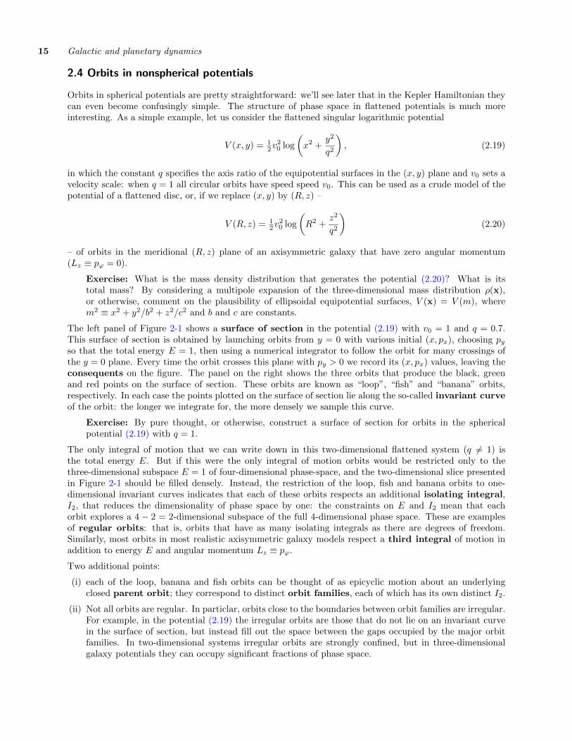
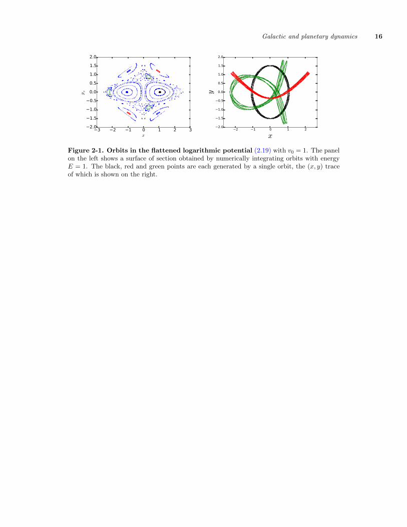
The left panel of Figure 2-1 shows a surface of section in the potential (2.19) with v0 = 1 and q = 0.7.This surface of section is obtained by launching orbits from y = 0 with various initial (x, px), choosing pyso that the total energy E = 1, then using a numerical integrator to follow the orbit for many crossings ofthe y = 0 plane. Every time the orbit crosses this plane with py > 0 we record its (x, px) values, leaving theconsequents on the figure. The panel on the right shows the three orbits that produce the black, greenand red points on the surface of section. These orbits are known as “loop”, “fish” and “banana” orbits,respectively. In each case the points plotted on the surface of section lie along the so-called invariant curveof the orbit: the longer we integrate for, the more densely we sample this curve.
Exercise: By pure thought, or otherwise, construct a surface of section for orbits in the sphericalpotential (2.19) with q = 1.
The only integral of motion that we can write down in this two-dimensional flattened system (q 6= 1) isthe total energy E. But if this were the only integral of motion orbits would be restricted only to thethree-dimensional subspace E = 1 of four-dimensional phase-space, and the two-dimensional slice presentedin Figure 2-1 should be filled densely. Instead, the restriction of the loop, fish and banana orbits to one-dimensional invariant curves indicates that each of these orbits respects an additional isolating integral,I2, that reduces the dimensionality of phase space by one: the constraints on E and I2 mean that eachorbit explores a 4 − 2 = 2-dimensional subspace of the full 4-dimensional phase space. These are examplesof regular orbits: that is, orbits that have as many isolating integrals as there are degrees of freedom.Similarly, most orbits in most realistic axisymmetric galaxy models respect a third integral of motion inaddition to energy E and angular momentum Lz ≡ pϕ.
Two additional points:
(i) each of the loop, banana and fish orbits can be thought of as epicyclic motion about an underlyingclosed parent orbit; they correspond to distinct orbit families, each of which has its own distinct I2.
(ii) Not all orbits are regular. In particlar, orbits close to the boundaries between orbit families are irregular.For example, in the potential (2.19) the irregular orbits are those that do not lie on an invariant curvein the surface of section, but instead fill out the space between the gaps occupied by the major orbitfamilies. In two-dimensional systems irregular orbits are strongly confined, but in three-dimensionalgalaxy potentials they can occupy significant fractions of phase space.
Galactic and planetary dynamics 16
−3 −2 −1 0 1 2 3x
−2.0
−1.5
−1.0
−0.5
0.0
0.5
1.0
1.5
2.0
px
−2 −1 0 1 2
x
−2.0
−1.5
−1.0
−0.5
0.0
0.5
1.0
1.5
2.0
y
Figure 2-1. Orbits in the flattened logarithmic potential (2.19) with v0 = 1. The panelon the left shows a surface of section obtained by numerically integrating orbits with energyE = 1. The black, red and green points are each generated by a single orbit, the (x, y) traceof which is shown on the right.
17 Galactic and planetary dynamics
3 Orbits: angle–action variables
3.1 Generating functions for canonical maps
We have already seen that the mapping obtained by drifting along the flow (1.40) generated by any functionB(q,p) is canonical. This is this most natural way of constructing maps that join smoothly onto theidentity map. But this produces only a subset of all canonical maps. For example, in §1.1 we constructedHamiltonians for a single particle, first using Cartesian (x, y, z) coordinates, then using spherical polars(r, ϑ, ϕ). Both sets of phase-space coordinates were canonical, but no mapping of the form (1.40) can relatethem.
To find a more general way of constructing maps, recall that the condition for a map
Qi = Qi(q,p),
Pi = Pi(q,p),(i = 1, . . . , n), (3.1)
to be canonical is that it preserves the Poincare integral invariants (1.64): that is, for any loops γ we musthave ∮
γ
p · q =
∮γ
P · dQ (3.2)
which means that the integrands can differ only by a total differential:
p · dq−P · dQ = dF, (3.3)
where F is some function defined on phase space. This F is the generating function of the transformationbetween (q,p) and (Q,P). It is an awkward, implicit way of specifying the transformation, but also verypowerful: from just one function of 2n phase-space coordinates we obtain a complete canonical map.
Type 1 generating functions Let us assume that we can express P = P(q,Q). Then we may eliminateP from F and write F = F1(q,Q), a function of both the old and new co-ordinates and time, but not themomenta. Substituting this F = F1 into (3.3) and using the chain rule gives
p · dq−P · dQ =∂F1
∂q· dq +
∂F1
∂Q· dQ. (3.4)
As (dq,dQ) can be varied independently (the equality above has to hold for any loop γ) we must have
p =∂F1
∂q, P = −∂F1
∂Q. (3.5)
Thus the function F1(q,Q) generates an implicit transformation from (q,p)→ (Q,P). By construction, itsatisfies the condition (3.2) and therefore is canonical.
Exercise: What mapping is generated by F1 = q ·Q? Show that the Hamiltonian H(q,p) = 12 (p2 +
ω2q2) is transformed to H(Q,P) = 12 (Q2 + ω2P2).
Type 2 generating functions Generating functions of the form F1(q,Q) are unsuitable for construct-ing mappings close to the identity. So, instead of writing F = F1(q,Q), let us take
F = −P ·Q + F2(q,P), (3.6)
in which we treat Q as a function Q(q,P). Substituting this into (3.2) and using the chain rule to expanddF gives:
p · dq−P · dQ = −Q · dP−P · dQ +∂F2
∂q· dq +
∂F2
∂P· dP. (3.7)
Galactic and planetary dynamics 18
As (dP,dq) vary independently, we must have that
p =∂F2
∂q, Q =
∂F2
∂P. (3.8)
This is another implicit canonical mapping between (q,p) and (Q,P).
Exercise: Show that F2(q,P) = q · P generates the identity map. What mapping does F2(q,P) =q ·P + εn · q produce? What about F2 = q ·P + εn ·P? What is the connection between this F2 andthe function B(z) that generates the phase flow (1.40)?
Exercise: Show that when the generating functions F1 or F2 depend on time t that the Hamiltoniantransforms to
K = H +∂F
∂t, (3.9)
where F is the appropriate GF and the (q,p) in the original H are expressed as q = q(Q,P) andsimilarly for p. Thus the canonical maps given by type-1 and type-2 generating functions are givenimplicitly by
F1(q,Q) : p =∂F1
∂q, P = −∂F1
∂Q, K(Q,P, t) = H(q,p, t) +
∂F1
∂t
F2(q,P) : p =∂F2
∂q, Q =
∂F2
∂P, K(Q,P, t) = H(q,p, t) +
∂F2
∂t.
(3.10)
3.2 Integrability: the Arnold-Liouville theorem and tori
An integral of motion I = I(q,p) is a function that commutes with the Hamiltonian: [I,H] = 0. Giventwo integrals of motion, I1(q,p) and I2(q,p), the Jacobi identity implies that [[I1, I2], H] = 0. So, [I1, I2] isanother integral of motion, albeit possibily a trivial one. For example, if Lx and Ly are integrals of motion,then so too is Lz.
If [I1, I2] = 0 then I1 and I2 are said to be in involution. That is, their phase flows commute. For example,in spherical systems the components of the angular momentum vector L = (Lx, Ly, Lz) are integrals ofmotion. The square of the total angular momentum L2 and any one of (Lx, Ly, Lz) are in involution, butany pair of Lx, Ly and Lz is not.
A Hamiltonian H for a system having n degrees of freedom is integrable if it has n independent integralsof motion, I1, ..., In, that are in involution with each other, [Ii, Ij ] = 0. The Hamiltonian itself is always oneof these integrals of motion.
Each such integral reduces dimension of accessible phase space by one, since Ii(q,p) = ci, where ci is aconstant. So motion in an integrable Hamiltonian is confined to an n-dimensional subvolume M of 2n-dimensional phase space. The Arnold–Liouville theorem states that, if this n-dimensional subvolume M iscompact, then
(i) M is (diffeomorphic to) an n-torus;
(ii) we can construct a coordinate system θ = (θ1, ..., θn) to label points in M , with each θi being 2π-periodic and increasing linearly with time, θi = Ωi.
See §49 of Arnold for the proof. The important idea is that each integral I1, ..., In defines a flow on M . Starting
from any point x0 ∈M we can reach some other x ∈M by drifting for some time t1 along the flow generated by
I1, followed by time t2 drifting along the flow generated by I2 and so on. Since the flows commute, the order inwhich we take them to travel from x0 to x does not matter. So these t = (t1, ..., tn) can be used to label (at least
some) points x ∈M . The torus-like nature of M follows by noticing that the domain of (t1, ..., tn) is Rn whereasM itself is compact by assumption. For certain choices t0 of t we must return to x0. These fixed points t0define a regular lattice on the domain Rn of t. The angles θi and corresponding constant frequencies Ωi are then
constructed by mapping the volume within a fundamental cell of this lattice onto the direct product of n unitcircles.
19 Galactic and planetary dynamics
So, these angle coordinates θ = (θ1, ..., θn) label points within the torus. We could label each torus bythe values (I1, ..., In) of the n integrals of motion, but it is better to use the Poincare invariants
Ji ≡1
2π
∮γi
p · dq, (3.11)
where γi is any closed loop that involves incrementing θi by 2π, with all other θj returning to their originalvalues. (A generalisation of Stokes’ theorem means that this integral is independent of the precise path takenby γi.) There are n such integrals, because any n-dimensional torus admits n independent loops that can’tbe deformed into one another. The J1, ..., Jn defined in (3.11) are the actions of the torus. The actions arefunctions Ji = Ji(I1, ..., In) of the original integrals of motion.
The (θ,J) coordinates are canonical: the mapping (q,p) ↔ (θ,J) is described by the type-2 generatingfunction (3.6)
F2(q,J) = S(q,J) =
∫ q
q0
p(q′,J)dq′, (3.12)
where q0 is some arbitrary reference point. It is immediately obvious that p = ∂S/∂q. To show that eachθi = ∂S/∂Ji, integrate along any loop γi along which θi increases by 2π with the other θj returning to theirinitial values. From (3.12) and (3.11) the quantity S increases by ∆S = Ji and so
∮p · dq =
∮J · dθ.
Let’s take the value c1 = E of the Hamiltonian H(q,p) as the first of the n integrals of motion. Then S(q,J)must satisfy the Hamilton–Jacobi equation,
H
(q,∂S
∂q
)= E, (3.13)
in which it is understood that J is held fixed. Solving this first-order PDE for S(q,J) allows us to constructmappings to action–angle variables (θ,J) given a Hamiltonian H(q,p).
In summary, if a Hamiltonian H(q,p) is integrable, then we can carry out a canonical map (q,p)→ (θ,J)to new phase-space coordinates in terms of which the Hamiltonian becomes H = H(J) and the equations ofmotion are simply
J = 0, θ = Ω, (3.14)
where the vector of frequencies,
Ω ≡ ∂H
∂J, (3.15)
gives the rate at which the system whizzes around the torus labelled by the actions J. This torus is sometimescalled an invariant torus because a trajectory that starts on the torus remains on it.
3.3 Angle–action variables for the simple harmonic oscillator
As an example, consider the Hamiltonian H(q, p) = 12p
2 + 12ω
2q2. The Hamilton–Jacobi equation (3.13) forS(q, J) in this case is
12
(∂S
∂q
)2
+ 12ω
2q2 = E, (3.16)
which yields∂S
∂q= ±
∫ [2E − ω2q2
]1/2dq. (3.17)
Substituting q = (√
2E/ω) sinu and integrating,
S(q, J) =E
ω(u+ 1
2 sin 2u) + F (J), (3.18)
Galactic and planetary dynamics 20
where F (J) is an arbitrary function of J . The variable u changes by 2π as we move around one completeorbit. The corresponding increase in S is 2πE/ω. Then by (3.11), the action integral for this orbit is
J =1
2π
∮∂S
∂qdq =
1
2π
∮∂S
∂udu =
E
ω. (3.19)
Expressed as a function of J , the Hamiltonian is therefore
H(J) = ωJ, (3.20)
and, from (3.18), the generating function is
S(q, J) = J(u+ 12 sin 2u) + F (J), (3.21)
in which u(q, J) is given implicitly by q =√
2J/ω sinu. The only effect of the arbtirary F (J) is to set the“origin” of the angle coordinate θ = 0. Choosing F = 0, the angle conjugate to J is given by
θ =∂S
∂J= u+ 1
2 sin 2u+ J(1 + cos 2u)∂u
∂J
∣∣∣∣q
= u+ 12 sin 2u− (1 + cos 2u)
cosu
sinu
= u.
(3.22)
Using p = ∂S/∂q = J(1 + cos 2u)(∂u/∂q)|J , the transformation from (θ, J) to (q, p) is
q =
√2J
ωsin θ, p = ω
√2J
ωcos θ. (3.23)
3.4 Angle–action variables for spherical potentials
We can use the same procedure we used in §3.3 to construct angle–action variables for any system withtwo or more degrees of freedom provided we can find a coordinate system in which the Hamilton–Jacobiequation (3.13) separates the sum
n∑i=1
Hi
(qi,
∂Si∂qi
)= E, (3.24)
in which
S(q,J) =
n∑i=1
Si(qi,J). (3.25)
Unfortunately, most Hamiltonians are not separable, which means that we have to find alternative methods toconstruct angle–action variables for them. The most important class of Hamiltonian for which the Hamilton–Jacobi separates are those for spherically symmetric potentials.
Taking q = (r, ϑ, ϕ), consider the Hamiltonian (1.14),
H(r, ϑ, pr, pϑ, pϕ) =1
2
[p2r +
p2ϑ
r2+
p2ϕ
r2 sin2 ϑ
]+ V (r), (3.26)
which on inspection has three independent integrals of motion in involution: H, pϕ and p2ϕ + p2
ϑ/ sin2 ϑ.Writing S(q,J) = Sr(r,J) + Sϑ(ϑ,J) + Sϕ(ϕ,J), the Hamilton–Jacobi equation is
1
2
[(∂Sr∂r
)2
+1
r2
(∂Sϑ∂ϑ
)2
+1
r2 sin2 ϑ
(∂Sϕ∂ϕ
)2]
+ V (r) = E, (3.27)
21 Galactic and planetary dynamics
which, separating variables in the usual way, yields the pair of separation constants
L2z =
(∂Sϕ∂ϕ
)2
= p2ϕ,
L2 =
(∂Sϑ∂ϑ
)2
+L2z
sin2 ϑ= p2
ϑ +p2ϕ
sin2 ϑ,
(3.28)
which are just the z component of angular momentum and the square of the total angular momentum. Theseare related to E by
1
2
[(∂Sr∂r
)2
+L2
r2
]+ V (r) = E. (3.29)
We choose Lz to have the same sign as pϕ, and L to be positive.
Around one complete cycle of ϕ, Sϕ increases by 2πpϕ, so the azimuthal action
Jϕ = Lz = pϕ. (3.30)
The variables (ϑ, pϑ) circulate around the loop given by L2 = p2ϑ + L2
z/ sin2 ϑ, in which ϑ is limited to theregion sinϑ > |Lz|/L ≡ sinϑmin. Over the course of one cycle Sϑ increases by
∆Sϑ = 4
∫ π/2
ϑmin
∂Sϑ∂ϑ
dϑ = 4
∫ π/2
ϑmin
[L2 − L2
z
sin2 ϑ
]1/2
dϑ
= 2π(L− |Lz|),(3.31)
and the latitudinal action is thereforeJϑ = L− |Lz|. (3.32)
Similarly, the radial action is
Jr =1
π
∫ r+
r−
[2(E − V )− L2
r2
]1/2
dr, (3.33)
where r− and r+ are the orbit’s peri- and apo-centre radii respectively.
The angles conjugate to these actions are θi = ∂S/∂Ji, where
S(q,J) = Sr(r, Jr, Jϑ, Jϕ) + Sϑ(ϑ, Jϑ, Jϕ) + Sϕ(ϕ, Jϕ). (3.34)
Using ∂S/∂qi = pi, the individual terms in the generating function can be written as
Sϕ(ϕ, Jϕ) =
∫ ϕ
0
Lzdϕ,
Sϑ(ϑ, Jϑ, Jϕ) =
∫ ϑ
π/2
±[L2 − L2
z
sin2 ϑ
]1/2
dϑ,
Sr(r, Jr, Jϑ, Jϕ) =
∫ r
r−
±[2(E − V (r′))− L2
r′2
]1/2
dr′,
(3.35)
in which the signs should be chosen to ensure that the integrals increase along an orbit. Notice that toeach of these functions we are free to add an arbitrary function of the actions and the other two angles.Doing that would simply move the location of the reference point θ = 0. The choice (3.35) places θ = 0 atpericentre, with (r, ϑ, ϕ) = (r−,
π2 , 0).
Galactic and planetary dynamics 22
Substituting (3.35) into the Hamilton–Jacobi equation (3.27) shows that radial action and the magnitude ofthe angular momentum L. Therefore
H = H(Jr, Jϑ + |Jϕ|), (3.36)
and the magnitudes of the azimuthal and latitudinal frequencies are equal, |Ωϑ| = |Ωϕ|. So, the quantityθϑ − sgn(Jϕ)θϕ an integral of motion in addition to (Jr, Jϑ, Jϕ).
Angle-action coordinates are not unique, however: we can construct new angle-action variables by takingappropriate linear combinations of the old ones. Let A be a 3 × 3 matrix with integer coefficients havingunit determinant. Then the map
J′ = (A−1)TJ, θ′ = Aθ, (3.37)
to new coordinates (θ′,J′) is canonical (exercise: why?). Moreover, increasing any one of the θ′i by 2π definesa distinct closed loop on the torus, so the new (θ′,J′) are angle–action coordinates. Let us use this map toconstruct the following new angle–action coordinates (θ′,J′) = (θ1, θ2, θ3, J1, J2, J3):
J1 = Jϕ = Lz,
θ1 = θϕ − sgn(Jϕ)θϑ,
J2 = Jϑ + |Jϕ| = L,
θ2 = θϑ,
J3 = Jr,
θ3 = θr.(3.38)
In these coordinates H = H(J2, J3), so that the angle θ1 becomes a fourth integral of motion in addition to(J1, J2, J3).
To understand the connection between these new coordinates and the orbital elements introduced in §2.3above, notice from (2.18) that the magnitude of cos i gives the magnitude of the projection of the angularmomentum L onto the z-axis, with the sign chosen so that Jϕ > 0 when i < π
2 . Therefore
cos i =J1
J2. (3.39)
The angles θi (i = 1, 2, 3) are given by θi = ∂S/∂Ji, where the generating function (3.34–3.35),
S(r, ϑ, ϕ, J1, J2, J3) = J1ϕ+
∫ ϑ
π/2
sϑ
[J2
2 −J2
1
sin2 ϑ
]1/2
dϑ+
∫ r
r−
sr
[2(H(J2, J3)− V (r′))− J2
2
r′2
]1/2
dr′,
(3.40)with the signs sϑ = ±1, sr = ±1 chosen to ensure that the integrals increase monotonically along the orbit.Consider the orbit just after it has passed upwards through the plane z = 0, so that z > 0 and ϑ < 0. Thensϑ = −1. Differentiating (3.40),
θ1 =∂S
∂J1= ϕ+ sgn(J1)
∫ ϑ
π/2
dϑ
sinϑ√
sin2 ϑ/ cos2 i− 1
= ϕ+ sgn(J1)1
sgn cos i
∫ sin−1(cot i cotϑ)
0
d[sin−1(cot i cotϑ)]
= ϕ− u,
(3.41)
where u is given by sinu = cot i cotϑ. From (2.18) or from Figure 3.26 of BT or Figure 10.7 of Goldstein,Poole & Safko (2002) it follows that this cot i cotϑ is equal to sin(ϕ − Ω) and, checking signs, u = ϕ − Ω.Therefore θ1 = Ω, the longitude of the ascending node.
23 Galactic and planetary dynamics
3.5 Angle–action variables for the Kepler Hamiltonian: Delaunay elements
Taking V (r) = −GM/r in (3.26) gives the Kepler Hamiltonian. In this case radial action can be calculatedanalytically. It is
Jr = 1π
∫ r+
r−
√2
(E +
GM
r
)− L2
r2dr =
GM√−2E
− L. (3.42)
Therefore the Kepler Hamiltonian is a very simple function of the actions, namely
H = − (GM)2
2(Jr + Jϑ + |Jϕ|)2= − (GM)2
2(Jr + L)2. (3.43)
This becomes the even simpler
H = − (GM)2
2J2c
, (3.44)
when we use (3.37) to define a third set of angle–action variables, (θa, θb, θc, Ja, Jb, Jc) through
Ja = Jϕ = Lz,
θa = θϕ − sgn(Jϕ)θϑ,︸ ︷︷ ︸(H,h)
Jb = Jϑ + |Jϕ| = L,
θb = θϑ − θr,︸ ︷︷ ︸(G,g)
Jc = Jr + L,
θc = θr.︸ ︷︷ ︸(L,l)
(3.45)
These new angle–action coordinates are in fact the Delaunay elements of the orbit: the underbraces in theequation above give the more usual labels for these variables. Notice that the frequencies are Ωa = Ωb = 0,Ωc = (GM)2/J3
c .
There is a simple relationship between these Delaunay elements and the orbital elements introduced in §2.3.Clearly J2
c = GMa and J2b = GMa(1 − e)2, so that J2
a = GMa(1 − e2) cos2 i. To understand the angles,apply θi = ∂S/∂Ji to to the generating function (3.34) and (3.35),
S(r, ϑ, ϕ, Jr, Jϑ, Jϕ) =
∫pr(r, Jr, Jϑ, Jϕ)dr +
∫pϑ(ϑ, Jϑ, Jϕ)dϑ+
∫pϕ(Jϕ)dϕ. (3.46)
to obtain θr = w, θϑ = ω − w, θϕ = Ω + sgn(Jϕ)θϑ, where w = η′ − e sin η′ is the mean anomaly. Therefore
Ja =√GMa(1− e2) cos i,
θa = Ω,︸ ︷︷ ︸(H,h)
Jb =√GMa(1− e2),
θb = ω,︸ ︷︷ ︸(G,g)
Jc =√GMa,
θc = w.︸ ︷︷ ︸(L,l)
(3.47)
A problem with Delaunay variables is that the angles (Ω, ω, w) are not well defined whenever i = 0 or e = 0.To remedy this, let us introduce modified Delaunay variables via
J$ =√GMa(1−
√1− e2),
θ$ = −(Ω + ω),︸ ︷︷ ︸(P,p)
JΩ =√GMa(1− e2)(1− cos i),
θΩ = −Ω,︸ ︷︷ ︸(Q,q)
Jλ =√GMa,
θλ = λ ≡ Ω + ω + w.︸ ︷︷ ︸(Λ,λ)
(3.48)
Here we have introduced two new angles,
(longitude of pericentre) $ ≡ ω + Ω,
(mean longitude) λ ≡ Ω + ω + w.(3.49)
λ is always well defined, whereas $ and Ω are undefined when the corresponding action is zero: these arepolar coordinates. Notice that
J$ ∝ e2, e 1,
JΩ ∝ i2, i 1.(3.50)
Galactic and planetary dynamics 24
3.6 (To note) the isochrone
The isochrone potential is
Φ(r) = − GM
b+√b2 + r2
. (3.51)
In the limit b → 0 this becomes the Kepler potential, whereas in the limit b → ∞ it becomes the sphericalsimple harmonic oscillator. The isochrone is important because it is the most general poetntial for which allangle–action variables can be obtained analytically from the ordinary phase-pace coordinates (x,p). We donot cover it explicitly in these lectures, but refer the reader to BT for details.
Why the name? In this potential the radial period of an orbit having energy E per unit mass is Tr =2πGM/(−2E)3/2, which is independent of angular momentum.
3.7 (To note) Staeckel potentials
Staeckel showed that only coordinate system in which the Hamiltonian–Jacobi equation H = 12p2+Φ(x) = E
separates is confocal ellipsoidal coordinates, of which Cartesian, spherical polar and cylindrical polars arejust limiting cases. Confocal spheroidal coordinates (u, v, ϕ) are the axisymmetric version. They are relatedto cylindrical coorindates via
R = ∆ sinhu sin v,
z = ∆ coshu cos v.(3.52)
If the potential is of the form
Φ(u, v) =U(u)− V (v)
sinh2 u+ sin2 v, (3.53)
for some functions U(u) and V (v), then it is easy to show that the Hamilton–Jacobi equation separates,providing two action integrals in addtion to Jϕ = Lz. Axisymmetric potentials of the form (3.53) are knownas Staeckel potentials. For more on Staeckel potentials and their applications to galaxy dynamics, see deZeeuw (1985).
3.8 Testing for integrability
Two degrees of freedom: plot surfaces of section. Three degrees of freedom: it’s NAFF: BT §3.7.
3.9 Numerical construction of angle–action variables
How to construct angle–action variables for more general Hamiltonians H(x,p)? One way is to start from a“toy” Hamiltonian H ′(J′,θ′) for which we can map easily between (x,p) and (θ′,J′). An example of sucha toy Hamiltonian is that of the isochrone model in §3.6. Having chosen H ′, we construct canonical mapbetween these toy coordinates (θ′,J′) and the angle–action coordinates (θ,J) of the target H as follows.Exploit the periodicity of the angle variables and represent the map by a type-2 generating function
S(θ′,J) = θ′ · J +∑n
Sn(J)ein·θ′ , (3.54)
so that
J′ =∂S
∂θ′= J +
∑n
inSn(J)ein·θ′ ,
θ =∂S
∂J= θ′ +
∑n
∂Sn
∂J(J)ein·θ′ .
(3.55)
25 Galactic and planetary dynamics
Note that Sn(J) = S?−n(J) if S is to be real.
Here is one way of choosing the coefficients Sn(J) that specify this generating function. We start by choosing avalue of J and setting up a regular grid in toy angles θ′. For given choice of Sn then the first of equations (3.55)gives the corresponding toy actions. We can use the toy Hamiltonian H0 to turn these (θ′,J′) into values of(q,p) and then to values of our target H(q,p). By adjusting the coefficents Sn to minimise the spread inthe values of H(q,p) we construct a mapping that lies on the torus of action J generated by H.
An alternative is is to use numerical orbit integration in the target H. This sets J, albeit implicitly. Usetoy Hamiltonian H ′ to turn the (q,p) from the orbit integration into toy variables (θ′,J′). Then, writingθ = Ωt, (3.55) is a set of linear simultaneous equations for Ω, J, Sn and their derivatives ∂Sn/∂J.
A third way is to average the first of equs (3.55) over toy angles θ′, obtaining J = 1(2π)3
∫J′ dθ′. The problem
reduces to carrying out this integral numerically given irregularly sampled points in θ′.
Here we’ve just touched on the general idea, but success depends on details such as the choice of toyHamiltonian H ′ and limiting |n|. Sanders & Binney (2016) review action-estimation methods in galacticdynamics.
3.10 Resonances and degeneracy
Apart from some special situations, the frequencies Ω are in general incommensurable: that is, the onlyvector of integers k ≡ (k1, ..., kn) for which k ·Ω = 0 is the trivial k = 0. The motion is then quasi-periodicor non-resonant. Given any function f(θ) on the torus, it follows then by expanding f(θ) =
∑k fkeik·θ
that the mean value of f averaged over the torus is
〈f〉θ =1
(2π)n
∫f(θ)dnθ =
1
(2π)n
∑k
fk
∫eik·θdnθ = f0, (3.56)
where f0 is the k = 0 component in the Fourier expansion of f(θ). On the other hand, using θ(t) = Ωt+ θ0
the time averaged value of the function f(θ(t)) is
〈f〉T ≡ limT→∞
1
T
∫ T
0
f(θ(t))dt = limT→∞
1
T
∫ T
0
∑k
fkei(Ωt+θ0)
= f0 + limT→∞
1
T
∑k6=0
fkeiΩT − 1
iΩ · k= f0,
(3.57)
provided there is no k for which k ·Ω 6= 0. That is, the time average of a function defined on a nonresonanttorus is equal to its angle average. In particular, the length of time that an orbit spends within an chunk Vof the torus is proportional to the volume occupied by V . A consequence of this is that any single orbit fillsthe torus densely: starting from any θ0, we come arbitrarily close to any other θ in the limit t→∞.
If there are m independent nonzero integer vectors, k1, ...,km for which ki ·Ω = 0 then the torus is resonantwith multiplicity m. Defining
|ki| ≡ |ki1|+ · · ·+ |kin|, (3.58)
the order of the resonance is the minimum value of |k1|, ..., |km|. In the extreme case m = n−1 the torusis completely resonant and the motion is periodic: after a finite length of time it repeats itself exactly.
For most Hamiltonians, adjusting J changes the vector of frequencies Ω. But if H is linear in the Ji then Ωis independent of J and the Hamiltonian is isochronous. More generally, if
det
(∂Ωi∂Jj
)= det
(∂2H
∂Ji∂Jj
)(3.59)
vanishes, the system is degenerate: there is at least one direction in J space along which Ω does notchange. Conversely, if H is nondegenerate then there is at least one direction along which Ω does change.Resonances k ·Ω = 0 are dense in the phase space of nondegenerate systems.
Galactic and planetary dynamics 26
4 Perturbation theory
Suppose that we have constructed angle–action variables for the Hamiltonian H0. As we have seen, Hamil-ton’s equations are then simply
J = 0, θ = Ω(J), (4.1)
where the angles θ increase at the rate Ω(J) = ∂H0/∂J.
Now add a perturbation εH1 to our original H0, where ε is a small parameter. Our mastery of angle–actionvariables means that we can express H1 = H1(θ,J). Hamilton’s equations for this perturbed system are
θ = Ω(J) + εf(θ,J), J = εg(θ,J), (4.2)
with f = ∂H1/∂J and g = −∂H1/∂θ. Our mastery does not extend, however, to constructing angle–actionvariables for the new Hamiltonian H0 + εH1, which depends on θ as well as J. On the other hand, weare usually more interested in the long-term behaviour of the system (e.g., in how the semimajor axes andeccentricities of the planets evolve) than in the details of how the rapidly varying angles θ change. It turnsout that the averaged system,
J = εg(J), (4.3)
where
g(J) ≡ 1
(2π)n
∫g(θ,J)dnθ, (4.4)
is often a good approximation to the evolution produced by the original equations (4.2). This is an ancientidea: when studying perturbations of planets, Gauss proposed to distribute the mass of each planet propor-tionally to the fraction of time it spent in each segment of the orbit. This reduces the solar system to asystem of interacting massive rings.
This averaging principle can be couched in more formal language (see §4.4 later), but for now let’s justassume that it works. To verify that there are cases for which it really does work, consider the toy exampleof a one-dimensional Hamiltonian H0 = H0(J) for which Ω = dH/dJ 6= 0. Apply a perturbation εg(θ),which for simplicity we take to be independent of J . Then the full solution to Hamilton’s equation J = εg is
J(t)− J(0) = ε
∫ t
0
g(θ0 + Ωt′)dt′
= εgt+ ε
∫ t
0
[g(θ0 + Ωt′)− g]dt′,
(4.5)
where θ0 is the initial angle. The second term in the RHS is a periodic function. Therefore it is bounded andthe evolution of J(t) consists of small oscillations (second term) superimposed on the long-term growth, εgt(first term). The averaged equation of motion (4.3) for this system is J = εg, which, although it ignores theoscillations on timescales . Ω−1, correctly captures the longer-term, secular evolution over many orbitalperiods.
We have not yet used the fact that the perturbation is (usually) Hamiltonian, so that g = −∂H1/∂θ.By the periodicity of H1 in the angles, we can write H1 =
∑k Sk(J)eik·θ for some Sk(J). Therefore
g(θ,J) = −i∑
k Sk(J)keik·θ and so g = 0: there should be no secular evolution in Hamiltonian systems!But this argument relies on the assumption that the averaging principle is approximately correct. This isnot true close to resonances, k ·Ω ' 0, which makes the dynamics vastly more interesting.
27 Galactic and planetary dynamics
4.1 The restricted three-body problem
Over the following few sections we’ll develop these ideas with application to the restricted three-body problemof a test particle (such as an asteroid or Pluto), moving in the combined potential of the sun plus a largeplanet (such as Jupiter or Neptune). We have already worked out the full Hamiltonian (1.29) for this systemin the general case, but in the restricted problem we focus on the motion of the test particle, imposingthe motion of the more massive sun and planet from without. So our first task is to obtain an effectiveHamiltonian for the test particle. Let the positions of the sun, large planet and test particle referred to aninertial frame be x0, xp and x respectively and their masses be m0, mp and m. The equations of motion are
m0x0 =Gmpm0
|xp − x0|3(xp − x0) +
Gmm0
|x− x0|3(x− x0),
mpxp =Gm0mp
|x0 − xp|3(x0 − xp) +
Gmmp
|x− xp|3(x− xp),
mx =Gm0m
|x0 − x|3(x0 − x) +
Gmpm
|xp − x|3(xp − x).
(4.6)
Now introduce the heliocentric coordinates rp ≡ xp−x0 and r ≡ x−x0. By taking appropriate combinationsof (4.6) we find that
r = −Gm0r
|r|3+Gmp(rp − r)
|rp − r|3− Gmprp
|rp|3(4.7)
which corresponds to motion in the Hamiltonian H(r,p) = H0 + εH1, where
H0(r,p) = 12p2 − Gm0
|r|,
εH1(r; rp) = −Gmp
(1
|rp − r|− r · rp
|rp|3
).
(4.8)
Here H0 is just the Kepler Hamiltonian for a central mass m0. The perturbation H1 is composed of a directterm ∝ 1/|rp − r| due to the influence of the planet plus an indirect term ∝ r · rp that accounts for thenoninertial frame. Notice that H1 is smaller than H0 by a factor ∼ mp/m0, which may take as our definitionof the scale ε. In the limit mp → 0 (ε→ 0) the motion reduces to the simple Keplerian case.
[At this point it would make sense to set Gm0 = 1 and ε = mp/m0, followed by ap = 1 below. But let’s plodalong without doing that, if only to keep our frequencies clear.]
Exercise: Explain how one can obtain (4.8) directly from (1.29). [Hint: remember that (i) pn 6= mnrnin (1.29); (ii) we are free to add a total time derivative dΛ/dt to the Hamiltonian, where Λ(q,p) is anyfunction of the phase-space coordinates.]
4.2 Example: Lidov–Kozai oscillations
Now consider the even more special situation in which the test particle is much closer to the sun than theplanet (r rp) and suppose that the planet is on a circular orbit, but the test particle is not confined tothe orbital plane of the planet. The following is a simplified version of Tremaine (2014); see also Tremaine& Yavetz (2014).
Use |rp − r|2 = r2p − 2rp · r + r2 to expand the first term in the perturbation (4.8) as
1
|rp − r|=
1
rp
[1 +
2rp · r− r2
2r2p
+3
8
(2rp · r− r2
r2p
)2
+ · · ·
]. (4.9)
Galactic and planetary dynamics 28
Dropping a constant term, the perturbation is then
εH1 = −Gmp
(1
|rp − r|− rp · r|rp|3
)=Gmp
r3p
[12r
2 − 3(rp · r)2
2r2p
]+O(r3/r4
p). (4.10)
We need to average this over the motion of both the test particle and the planet. Let (e, u, n) be unit vectorsin a right-handed coordinate system centred on the sun with e pointing towards the pericentre of the testparticle (which has true anomaly ϕ = 0), u pointing towards ϕ = π/2 and n normal to the test particle’s
orbit plane. Let (ep, up, np) be corresponding unit vectors for the planet.† Then r = r(ϕ)(cosϕe + sinϕu)and rp = rp(ϕp)(cosϕpep + sinϕpup). Averaging (4.10) gives
εH1 =Gmp
a3p
[12 〈r
2〉 − 3〈cos2 ϕp〉2a2
p
(〈r2 cos2 ϕ〉(ep · e)2 + 〈r2 sin2 ϕ〉(ep · u)2
)− 3〈sin2 ϕp〉
2a2p
(〈r2 cos2 ϕ〉(up · e)2 + 〈r2 sin2 ϕ〉(up · u)2
) ],
(4.11)
where the triangular brackets denote time averages. By assumption the planet is on a circular orbit. So,〈cos2 ϕp〉 = 〈sin2 ϕp〉 = 1
2 . For the test particle we can express r in terms of the eccentric anomaly η throughr(η) = a(1− e cos η) and use Kepler’s equation w = η− e sin η to write time averages (i.e., averages over themean anomaly w) as integrals over η. The latter is defined via a(1− e cos η) = a(1− e2)/(1 + e cosϕ), fromwhich it follows that
cosϕ =cos η − e
1− e cos η, sinϕ =
√1− e2 sin η
1− e cos η. (4.12)
Therefore the averages that appear in εH1 are
〈r2〉 = a2(1 + 3
2e2), 〈r2 cos2 ϕ〉 = 1
2a2(1 + 4e2), 〈r2 sin2 ϕ〉 = 1
2a2(1− e2), (4.13)
and so the averaged perturbation becomes
εH1 =Gmpa
2
4a3p
[2 + 3e2 − 3
2 (1 + 4e2)(ep · e)2 − 32 (1− e2)(ep · u)2
− 32 (1 + 4e2)(up · e)2 − 3
2 (1− e2)(up · u)2
]
=Gmpa
2
4a3p
[2 + 3e2 − 3
2 (1 + 4e2)((ep · e)2 + (up · e)2
)− 3
2 (1− e2)((ep · u)2 + (up · u)2
) ].
(4.14)
Now use the relations (ep · e)2 + (up · e)2 + (np · e)2 = 1 and (ep · u)2 + (up · u)2 + (np · u)2 = 1 to eliminatethe dependence of εH1 on ep and up. The result is
εH1 =Gmpa
2
4a3p
[− 1− 3
2e2 + 3
2 (1 + 4e2)(np · e)2 + 32 (1− e2)(np · u)2
]. (4.15)
We define the orbital elements of the test particle with reference to the orbital plane of the planet. Thennp · e = sin i sinω and np · u = sin i cosω from (2.16), and
εH1 =Gmpa
2
8a3p
[1− 6e2 − 3(1− e2) cos2 i+ 15e2(1− cos2 i) sin2 ω
]
=Gmpa
2
8a3p
[− 5 + 6
J2b
J2c
− 3J2a
J2c
+ 15
(1− J2
b
J2c
)(1− J2
a
J2b
)sin2 θb
],
(4.16)
† (Just in case you feel inspired to generalize to the case in which the perturbing planet is on a noncircular orbit...)

29 Galactic and planetary dynamics
0.0 0.2 0.4 0.6 0.8 1.0ω/π
0.0
0.2
0.4
0.6
0.8
e
Figure 4-1. Lidov–Kozai oscillations Level surfaces of the Lidov–Kozai averaged Hamil-tonian (4.18) for C = 1
2 .
when expressed in terms of the Delaunay elements (3.45): recall that Jb is the total angular momentum,which you’d normally call L (but which celestial mechanics might label G; they keep the label L for Jc.).
The unperturbed Hamiltonian H0 = H0(Jc). Averaging H = H0 +εH1 over θc we’re left with Jc =√GMa =
constant and Ja =√GMa(1− e2) cos i = constant. The dynamics are then determined by the level surfaces
of (4.16) as a function of (θb, Jb). The semi major axis a is constant, but orbits can trade eccentricity e forinclination i, with
cos i = cos i0
√1− e2
0
1− e2, (4.17)
where (e0, i0) are the initial values of (e, i). Eliminating cos i in favour of e, the averaged Hamiltonian (4.16)becomes
εH1 =Gmpa
2
8a3p
[1− 6e2 − 3C + 15e2
(1− C
1− e2
)sin2 ω
], (4.18)
where the constant C = (1− e20) cos2 i0. Figure 4-1 shows the level surfaces of this εH1 for (e0, i0) = (0, 60).
Suppose that the test particle starts on a circular orbit e0 = 0 with inclination i0. Conservation of εH1
implies either that e = 0 (particle remains on a circular orbit) or that
2(1− e2) + 5(e2 − sin2 i0) sin2 ω = 0, (4.19)
in which case it executes Lidov–Kozai oscillations about ω = ±90. It is easy to see from (4.19) that thecondition for these oscillations to be possible is that sin2 i0 > 2/5, or i0 > 39.2. The maximum eccentricityof emax = [(5 sin2 i0 − 2)/3]1/2 occurs at ω = ±90.
Notice that the existence of these oscillations is independent of the strength of the perturbation from thedistant planet: changing the prefactor in (4.18) just changes the period of the oscillations. So, an arbitrarilysmall external force can in principle excite these oscillations.
Perhaps the most “down-to-earth” application of these oscillations is the stability of artificial satellitesorbiting the earth. There the moon acts as the “distant perturber”, but a more complete model of theirmotion would account for the additional perturbation due to the flattening of the earth: see Tremaine &Yavetz (2014).
Galactic and planetary dynamics 30
4.3 When average is not good enough: resonances
Now let us consider a different regime of the restricted three-body problem. Suppose that the test particleand planet both move in the same plane, but relax the assumption that the test particle is much closer tothe central star than the planet. Let φ = cos−1(r ·rp/rrp) be the angle between them. Using the cosine rule,
εH1 = −Gmp
rp
(1 +
(r
rp
)2
− 2
(r
rp
)cosφ
)−1/2
−(r
rp
)cosφ
. (4.20)
We want to be able to express this in terms of the angle-action variables for H0, or, equivalently, in termsof semi-major axis a and eccentricity e. The result is (4.30) below, but it is worth being aware of some ofthe gory details of how this expansion can be carried out in practice.
Recall that r = a(1− e cos η) and rp = ap(1− ep cos ηp), where η and ηp are eccentric anomalies. Therefore
r
rp=
a
ap(1− e cos η + ep cos ηp) +O(e2), (4.21)
which we now use to expand εH1 to first order in e. Introducing α ≡ a/ap and Taylor expanding H1,
εH1 = −Gmp(1− ep cos ηp)
ap
[ (1 + α2 − 2α cosφ
)−1/2
+ (α− cosφ)α (e cos η − ep cos ηp)(1 + α2 − 2α cosφ
)−3/2
− α(1− e cos η + ep cos ηp) cosφ
]+O(e2).
(4.22)
The powers of (1 + α2 − 2α cosφ) in this expression can be Fourier expanded as
[1 + α2 − 2α cosφ
]−s=
∞∑j=−∞
b(j)s cos jφ. (4.23)
where the Laplace coefficients,
b(0)s (α) ≡ 1
π
∫ π
0
dφ
(1 + α2 − 2α cosφ)s,
b(j)s (α) ≡ 2
π
∫ π
0
cos jφ dφ
(1 + α2 − 2α cosφ)s, (j 6= 0),
(4.24)
can be treated as standard functions. Expressed in terms of them, the perturbation Hamiltonian becomes
εH1 = −Gmp(1− ep cos ηp)
ap
[ ∞∑j=−∞
b(j)1/2(α) cos jφ
+ (α− cosφ)α (e cos η − ep cos ηp)
∞∑j=−∞
b(j)3/2(α) cos jφ
− α(1− e cos η + ep cos ηp) cosφ
]+O(e2).
(4.25)
Now we need to rewrite the cos jφ and e cos η factors that appear here in terms of the modified Delaunayangles (3.48) θ = (θ$, θΩ, θλ) = (−$,−Ω, λ). The mean anomaly w ≡ η − e sin η so that
cosw = cos η + e sin2 η +O(e2). (4.26)
31 Galactic and planetary dynamics
Then the factor e cos η = e cosw+O(e2) = e cos(λ−$)+O(e2). To deal with the cos jφ factors, notice that theangle φ = ϕ+$−(ϕp +$p), where ϕ and ϕp are the true anomalies of the test body and planet respectively.These are related to the eccentric anomalies η and ηp through r = a(1 − e2)/(1 + e cosϕ) = a(1 − e cos η),which gives
cosϕ =cos η − e
1− e cos η= cos η − e sin2 η +O(e2) (4.27)
and therefore sinϕ = sin η + e sin η cos η +O(e2). Then it is easy to verify that
ϕ = η + e sin η +O(e2) = w + 2e sinw +O(e2) (4.28)
and so thatcos j(ϕ+$) = cos j(w +$)− 2je sinw sin j(w +$) +O(e2)
= cos jλ− 2je sin(λ−$) sin jλ+O(e2),(4.29)
with a similar expression for sin j(ϕ+$). The mean longitude λp of the planet increases linearly with time,λp = Ωλp
t, where Ωλpis related to the period Tp of the planet through Ωλp
= 2π/Tp. Then the perturbationHamiltonian becomes
εH1(λ,$, a, e;$p, ap, ep, t) = −Gmp
ap
∑jkl
Cjkl(a, e; ap, ep)ei(j$+kλ+lΩλp t), (4.30)
where the functions Cjkl can be found by substituting the expressions for cosw, cos j(ϕ + $) and so oninto (4.25) and replacing the resulting products of trig functions by sums and differences. Note that thequantities $p, ap, ep in this expression are fixed parameters, not dynamical variables.
We can remove the explicit time dependence by adding a term ΩλpJλp to our unperturbed H0 and extendingthe phase space to include λp. The full Hamiltonian is therefore
H(λ,$, Jλ, J$, λp) = −1
2
(Gm0
Jλ
)2
+ ΩλpJλp︸ ︷︷ ︸
H0
−Gmp
ap
∑jkl
Cjkl(Jλ, J$; ap, ep)ei(j$+kλ+lλp)
︸ ︷︷ ︸εH1
. (4.31)
The equations of motion are
J$ = − ∂H
∂(−$)= −Gmp
api∑jkl
jCjklei(j$+kλ+lλp),
Jλ = −∂H∂λ
= +Gmp
api∑jkl
kCjklei(j$+kλ+lλp),
−$ = θ$ =∂H
∂J$= −Gmp
ap
∑jkl
∂Cjkl∂J$
ei(j$+kλ+lλp),
λ = θλ =∂H
∂Jλ=
[Gm0]2
J3λ
− Gmp
ap
∑jkl
∂Cjkl∂Jλ
ei(j$+kλ+lλp),
(4.32)
Integrating, say, the first of these equations taking quantities on the RHS along the unperturbed orbitλ = Ωλt+ const, λp = Ωλp
t+ const gives
J$(t) = −Gmp
ap
∑jkl
jCjklkΩλ + lΩλp
ei(kΩλ+lΩλp )tei(j$+const) + const, (4.33)
the denominator of which blows up whenever the frequencies Ωλ and Ωλpare close to resonance. The reason
is simple. The (j, k, l) component of the perturbation acts for a period T = 2π/(jΩ$ + kΩλ + lΩλp). The
longer this perturbation is applied, the stronger the deviation of the resulting orbit from its unperturbedform.
Exercise: The expression for εH1 involves the opaque functions Cjkl. By going back to (4.25), orotherwise, explain what happens in the special case of perfectly circular orbits (e = ep = 0).

Galactic and planetary dynamics 32
4.4 Perturbation theory using canonical maps
To understand how to deal with resonances we first need a slightly more nuanced way of treating theperturbation Hamiltonian εH1. In general, the perturbed problem can be described by a Hamiltonian
H0(θ0,J0) = H0(J0) + εH1(θ0,J0), (4.34)
where we are able to construct angle-action coordinates (θ0,J0) for some unperturbed Hamiltonian H0 andε is a small parameter that controls the size of the perturbation H1. For solar system problems H0 is theKepler Hamiltonian due to the sun and the dominant contribution in H1 is the perturbation due to Jupiter,which has a mass 10−3M. Therefore ε ∼ 10−3.
Idea: look for a canonical map, close to the identity, of the form
θ0 = θ1 + ε∆θ1(θ1,J1), J0 = J1 + ε∆J1(θ1,J1), (4.35)
in terms of which the Hamiltonian, expressed as a function of the new coordinates,
H1(θ1,J1) = H0(J1 + ε∆J1) + εH1(θ1 + ε∆θ1,J1 + ε∆J1), (4.36)
is independent of θ1 to first order in ε:
H1(θ1,J1) = H0(J1) + εH1(J1) + ε2H2(θ1,J1). (4.37)
For instance, H1 could be obtained by averaging (4.36) over θ1, with H2 scooping up the leftovers. Then,the equations of motion for our new first-order Hamiltonian H0(J1) + εH1(J1) are simply J1 = 0 and
θ1
= ∂∂J1 (H0 + εH1), which can be transformed back to our original (θ0,J0) coordinates using (4.35)
We can iterate this procedure. Let
θr−1 = θr + ε∆θr(θr,Jr), Jr−1 = Jr + ε∆Jr(θr,Jr). (4.38)
ThenHr(θr,Jr) = H0(Jr) + εH1(Jr) + · · ·+ εrHr(J
r) + εr+1Hr+1(θr,Jr), (4.39)
with each Hr and Hr+1 obtained by averaging the preceding Hr−1(θr−1,Jr−1) over the new θr.
Unfortunately this simple procedure does not work up to arbitrarily high order: resonances are unavoidable.A more immediate problem is that we need to ensure that the maps (4.35) and (4.38) are canonical.
33 Galactic and planetary dynamics
4.5 Lie transforms
The neat way to ensure that the maps are canonical is to use the fact that in the limit ε→ 0 they reduce tothe identity map. That is, they must be generated by some phase flow. Write zr = (θr,Jr). Then we canexpress (4.38) as
zr−1 = exp[εLχr ]zr (4.40)
and the problem reduces to finding a generating Hamiltonian χr that takes Hr to Hr−1. We focus on thefirst such generating Hamiltonian, χ1, and write z0(ε) = eεLχ1 z1.
Exercise: The Lie transform of the function f(z) under the flow generated by another function χ isdefined as f(z) ≡ f(eεLχz). Show that f = exp[εLχ]f .
Now use the fact that H0 and H1 refer to the the same perturbed Hamiltonian, just expressed in differentcoordinates. To make this distinction clear, write H (unadorned, without superscript) for the underlying(coordinate-free) Hamiltonian function and introduce a pair of (symplectic) coordinate maps, ϕ0 and ϕ1, sothat
H0(z0) = H ϕ0(z0),
H1(z1) = H ϕ1(z1).(4.41)
Clearly ϕ0(z0) = ϕ1(z1). Now consider two different ways of looking at the flow generated by χ1. One is thatχ1 has no effect on H itself, but instead changes the phase-space location of the point P = ϕ0(z0) = ϕ1(z1)that is fed to H. The output of the function after the flow has acted is then H ϕ1(eεLχ1 z1). Another viewis that the flow leaves P unchanged but modifies H, changing it to a new function eεLχ1H. In that case theresult of applying the function is (eεLχ1H) ϕ1(z1). These two outputs should be equal. So,
H ϕ1(eεLχ1 z1) = (eεLχ1H) ϕ1(z1). (4.42)
Using z0 = eεLχ1 z1 and ϕ1(z1) = ϕ0(z0) this becomes
H ϕ1(z0) = (eεLχ1H) ϕ0(z0). (4.43)
Replacing the argument z0 by z1 = (θ1,J1) and switching back to more conventional notation, we obtainour formal expression for H expressed in terms of the new coordinates:
H1(θ1,J1) = eεLχ1H0(θ1,J1). (4.44)
Substitute H0 = H0 + εH1 and expand, giving
H1 = H0 + ε[H0, χ1] + 12ε
2[[H0, χ1], χ1] +O(ε3)
= H0 + εH1 + ε[H0, χ1] + ε2[H1, χ1] + 12ε
2[[H0, χ1], χ1] +O(ε3),(4.45)
in which everything has arguments (θ1,J1).
Look at the O(ε) terms in this expression. Comparing to (4.37), the O(ε) factors agree if we take
H1 + [H0, χ1] = H1(J1). (4.46)
To find this generating Hamiltonian χ1, expand H1 and χ1 as Fourier series in the (new) angles:
H1(θ1,J1) =∑k
ck(J1)eik·θ1
,
χ1(θ1,J1) =∑k
dk(J1)eik·θ1
.(4.47)
Using H0 = H0(J1) from (4.37) and defining Ω0(J1) ≡ ∂H0/∂J1, we find that
[H0, χ1] = −i∑k
dk(J1)k ·Ω0(J1)eik·θ1
. (4.48)
Galactic and planetary dynamics 34
Then choosing coefficients
d0 = 0, dk(J1) = −ick(J1)
k ·Ω0(J1)(4.49)
gives H1 +[H0, χ1] = c0. That is, the mapping generated by the function χ1 in (4.47) with coefficients (4.49)annihilates the first-order dependence of H1 on the angles. The function
H1(J1) = c0(J1), (4.50)
which is just the perturbation H1(θ1,J1) averaged over θ1.
Resonances Notice the k · Ω(J1) in the denominator in the expression for dk: resonances or almostresonances between the components of the frequency vector Ω0 leads to the notorious “small denominators”problem. Let K be the resonant set of all integer vectors k for which k ·Ω0 = 0. Equation (4.48) shows that
all of the terms in [H0, χ1] involving eik·θ1
with k ∈ K vanish. No matter how we choose the coefficients dkin χ1, we cannot eliminate these resonant terms from the LHS of (4.46). So the RHS, H1, must depend on
the resonant terms eik·θ1
, k ∈ K, in addition to the actions J1. This first-order averaged Hamiltonian is
H1(θ1,J1) =∑k∈K
ck(J1)eik·θ1
, (4.51)
and the coefficients dk of the generator χ1 are given by
dk(J1) =
0, k ∈ K,
−i ck(J1)k·Ω0(J1) , otherwise,
(4.52)
instead of (4.49).
As an extreme example of such a resonant problem, consider the Kepler Hamiltonian. In modified Delaunaycoordinates, the frequency vector Ω = (Ω$,ΩΩ,Ωλ) with Ωλ 6= 0 and Ω$ = ΩΩ = 0. Then the set K ofresonant wavevectors is (j, k, 0), j, k ∈ Z and the averaged first-order Hamiltonian (4.51) is
H1(θ1$, θ
1Ω,J
1) =∑jk
cjk0(J1)ei(jθ1$+kθ1
Ω), (4.53)
in which cjk0 is obtained by averaging H1 over the longitude θλ. The generator of the map between (θ0,J0)and (θ1,J1) is
χ1 = −i∑jkll 6=0
cjkl(J1)
lΩλ(J1)ei(jθ1
$+kθ1Ω+lθ1
λ). (4.54)
4.6 Mr Lie applied to the restricted three-body problem
Now let us apply the Lie transform of §4.5 to kill off the O(ε) dependence of the Hamiltonian (4.31) onthe angle λ in the restricted three-body problem. In this case we cannot remove the dependence on $,because Ω$ = 0. Following the procedure of §4.5, the full the full Hamiltonian (4.31), expressed in the newcoordinates ($1, λ1, J1
$, J1λ), becomes
H1($1, λ1, J1$, J
1λ, λp) = H0(J1
λ, J1λp
) + εH1($1, J1$, J
1λ) +O(ε2), (4.55)
with
εH1 = −Gmp
ap
∑j
Cj00(J1)eij$1
, (4.56)
35 Galactic and planetary dynamics
obtained (see equ. (4.53)) by averaging the perturbation (4.30) over the angles λ1 = λ0 +O(ε) and λ1p. The
equations of motion in the new variables are
J1$ =
Gmp
api∑j
jCj00(J1)eij$1
,
J1λ = 0,
−$1 = −Gmp
ap
∑j
∂Cj00
∂J1$
eij$1
,
λ1 =Gm0
(J1λ)3− Gmp
ap
∑j
∂Cj00
∂J1λ
eij$1
.
(4.57)
Nothing much happens: J1λ is a constant, whereas (−$1, λ1, J1
$) just oscillate about their original values.These new variables (θ1
$, θ1λ, J
1$, J
1λ) are called mean modified Delaunay variables. By (4.47) and (4.52)
the generator of the map from them back to the orginal (θ0,J0) is
εχ1 = −iGmp
ap
∑jklkl 6=0
Cjkl
k [Gm0]2
(J1λ
)3 + lΩλp
ei(j$1+kλ1+lλ1p), (4.58)
using Ωλ = [Gm0]2/(J1λ)3 +O(ε). Then the mapping (4.40) for, e.g., J$ is
J0$ = J1
$ + ε[J1$, χ1] = J1
$ − ε∂χ1
∂(−$1)
= J1$ −
Gmp
ap
∑jklkl 6=0
jCjkl
k [Gm0]2
(J1λ
)3 + lΩλp
ei(j$1+kλ1+lλ1p),
(4.59)
which agrees to O(ε) with our earlier expression (4.33). Carrying out analogous mappings for the remainingangle-action coordinates, we obtain Jλ(t), λ(t) and $(t) which gives us the full set of orbit elements of theperturbed problem as a function of time. As in (4.33) this mapping fails when the frequencies Ωλ and Ωλp
of the test particle and planet are commensurate.
4.7 Dealing with resonances
We have just seen that, away from resonance, motion of a test body in the restricted three-body problem canbe expressed as a superposition of small oscillations on top of an underlying unperturbed Keplerian orbit.Now let us examine what happens close to resonance. Consider the case in which KΩ ' KpΩp. That is,for every K orbits the planet makes, the test body completes Kp. This is known as a Kp : K mean-motionresonance. For example, the Pluto–Neptune system has 3Ω = 2Ωp, so that K = 3, Kp = 2: they are ina 2 : 3 mean-motion resonance. Another example is provided by the Hilda asteroids, which are in a 3 : 2resonance with Jupiter. We assume that K 6= Kp in the following.
In the expansion (4.30) of H0 + εH1 let us focus on the (j, k, l) = (0, 0, 0) term plus the (j, k, l) = (j,K,−Kp)and (j,−K,Kp) resonant terms that lead to the small denominators problem. Some good news: we needonly a very restricted range of values of j. To see this, consider rotating the coordinate system by an angle∆ϕ about the z axis. This increases the Euler angle Ω by ∆ϕ, which, from (3.48), means that $, λ andλp increase by the same amount. But εH1 in (4.31) must be unchanged under such rotations. So we musthave j + k + l = 0. That is, j = −(k + l) = −(K −Kp) when k = +K, l = −Kp, and j = (K −Kp) whenk = −K. Then the resonant part of the perturbation can be written as
εH1 = −Gmp
ap[A(J) +B(J) cos((Kp −K)$ +Kλ−Kpλp + β)] , (4.60)
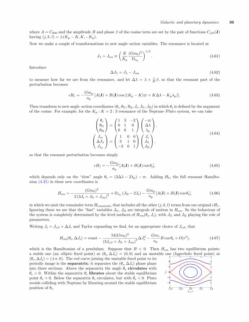
Galactic and planetary dynamics 36
where A = C000 and the amplitude B and phase β of the cosine term are set by the pair of functions Cjkl(J)having (j, k, l) = ±(Kp −K,K,−Kp).
Now we make a couple of transformations to new angle–action variables. The resonance is located at
Jλ = Jres ≡(K
Kp
(Gm0)2
Ωλp
)1/3
. (4.61)
Introduce∆Jλ = Jλ − Jres (4.62)
to measure how far we are from the resonance, and let ∆λ = λ + 1Kβ, so that the resonant part of the
perturbation becomes
εH1 = −Gmp
ap[A(J) +B(J) cos ((Kp −K)$ +K∆λ−Kpλp)] . (4.63)
Then transform to new angle–action coordinates (θs, θf1, θf2, Js, Jf1, Jf2) in which θs is defined by the argumentof the cosine. For example, for the Kp : K = 2 : 3 resonance of the Neptune–Pluto system, we can take θs
θf1
θf2
=
1 3 −20 1 00 0 1
−$∆λλp
,
J$∆JλJλp
=
1 0 03 1 0−2 0 1
Js
Jf1
Jf2
,
(4.64)
so that the resonant perturbation becomes simply
εH1 = −Gmp
ap[A(J) +B(J) cos θs], (4.65)
which depends only on the “slow” angle θs = (3∆λ − 2λp) − $. Adding H0, the full resonant Hamilto-nian (4.31) in these new coordinates is
Hres = − (Gm0)2
2 (3Js + Jf1 + Jres)2 + Ωλp (Jf2 − 2Js)−
Gmp
ap[A(J) +B(J) cos θs], (4.66)
in which we omit the remainder termHremainder that includes all the other (j, k, l) terms from our original εH1.Ignoring these we see that the “fast” variables Jf1, Jf2 are integrals of motion in Hres. So the behaviour ofthe system is completely determined by the level surfaces of Hres(θs, Js), with Jf1 and Jf2 playing the role ofparameters.
Writing Js = Js,0 + ∆Js and Taylor expanding we find, for an appropriate choice of Js,0, that
Hres(θs,∆Js) = const− 54(Gm0)2
(3Js,0 + Jf1 + Jres)4 ∆J2
s −Gm1
apB cos θs +O(ε2), (4.67)
−1.0 −0.5 0.0 0.5 1.0θslow/π
−2
−1
0
1
2
Jslow
which is the Hamiltonian of a pendulum. Suppose that B < 0. Then Hres has two equilibrium points:a stable one (an elliptic fixed point) at (θs,∆Js) = (0, 0) and an unstable one (hyperbolic fixed point) at(θs,∆Js) = (±π, 0). The red curve joining the unstable fixed point to itsperiodic image is the separatrix; it separates the (θs,∆Js) phase planeinto three sections. Above the separatrix the angle θs circulates withθs > 0. Within the separatrix θs librates about the stable equilibriumpoint θs = 0. Below the separatrix θs circulates, but with θs < 0. Plutoavoids colliding with Neptune by librating around the stable equilibriumposition of θs.
37 Galactic and planetary dynamics
4.8 Capture into resonance
4.9 Why does perturbation theory work?
4.10 Adiabatic invariants
Galactic and planetary dynamics 38
5 Galaxies: collisionless approximation
Timescales: dynamical time, relaxation.
N -particle DF fN (x1,v1, ...,xN ,vN , t) vs 1-particle DF f(x,v, t).
5.1 Collisionless Boltzmann equation
5.2 Moments of the DF: Jeans and virial equations
Jeans equations. Virial equations.
From N -body experiments, we see that galaxies settle down into approximate equilibrium (“virialise”) withina few dynamical times. This suggests that that a good way of understanding them is to think of them assome underlying equilibrium f(x,v),Φ(x) plus perturbations on top of this.
5.3 Jeans’ theorem
(Including strong Jeans’ thm)
5.4 Simple equilibrium galaxy models
5.5 Constructing constrained models
6 Dynamical evolution of galaxies