quantum mechanical free energy calculations using path
TRANSCRIPT

Quantum mechanical free energycalculations using path integral
molecular dynamics
by
Kevin P. Bishop
A thesispresented to the University of Waterloo
in fulfillment of thethesis requirement for the degree of
Doctor of Philosophyin
Chemistry
Waterloo, Ontario, Canada, 2019
c© Kevin P. Bishop 2019

Examining Committee Membership
The following served on the Examining Committee for this thesis. The decision of theExamining Committee is by majority vote.
External Examiner: Thomas MarklandAssociate Professor, Dept. of Chemistry, Stanford University
Supervisor: Pierre-Nicholas RoyProfessor, Dept. of Chemistry, University of Waterloo
Internal Member: Marcel NooijenProfessor, Dept. of Chemistry, University of Waterloo
Internal Member: William PowerAssociate Professor and Department Chair,Dept. of Chemistry, University of Waterloo
Internal-External Member: Jeff ChenProfessor, Dept. of Physics, University of Waterloo
iii


Author’s Declaration
This thesis consists of material all of which I authored or co-authored: see Statementof Contributions included in the thesis. This is a true copy of the thesis, including anyrequired final revisions, as accepted by my examiners.
I understand that my thesis may be made electronically available to the public.
v


Statement of Contributions
This thesis contains work that has been published or submitted for publication. Theseworks have been acknowledged in footnotes in the body of this thesis. My contributionsare summarized below.
K. P. Bishop, S. Constable, N. F. Faruk, P.-N. Roy, “OpenMM Accelerated MMTK”,Comput. Phys. Commun. 191, 203 (2015).
The material used in this thesis relating to this manuscript is solely my own.
W. S. Hopkins, P. J. Carr, D. Huang, K. P. Bishop, M. Burt, T. B. McMahon, V. Stein-metz, E. Fillion, “Infrared-Driven Charge Transfer in Transition Metal B12F12 Clusters”,J. Phys. Chem. A 119, 8469 (2015).
This manuscript is not used within this thesis. I performed the various DFT calculationsdescribed in this work.
T. Zeng, N. Blinov, G. Guillon, H. Li, K. P Bishop, P.-N. Roy, “MoRiBS-PIMC: A programto simulate molecular rotors in bosonic solvents using path-integral Monte Carlo”, Comput.Phys. Commun. 204, 170 (2016).
This manuscript is not used within this thesis. My contribution to this work wasprimarily the modification of the source code to ensure portability and the creation of theassociated user manual.
K. P. Bishop, P.-N. Roy, “Free energy calculations with post quantization restraints:binding free energy of the water dimer over a broad range of temperatures”, J. Chem.Phys. 148, 102303 (2018)
The material used in this thesis relating to this manuscript is solely my own.
K. P. Bishop, D. Iouchtchenko, and P.-N. Roy, “Free energy profiles from constrained pathintegral molecular dynamics: III. Water dimer with MB-pol” (Manuscript in preparation).
The material used in this thesis relating to this manuscript is solely my own.
vii


Abstract
Free energy calculations are one of the most powerful tools within modern theoreticalchemistry and are often used to make comparisons with experimental results. Existing freeenergy calculations are typically performed for classical molecular dynamics simulations butthere are certain systems where nuclear quantum effects play an integral role. Specifically,systems with light atoms or low temperatures are the most influenced by such nuclearquantum effects and the development of Feynman path integrals [1] has been effective inaccurately describing the quantum nature of these nuclei [2–8]. The primary objective ofthis thesis is the development of a pair of methodologies to calculate free energies utilizingpath integral molecular dynamics to account for nuclear quantum effects.
Prior to the development of these free energy methodologies, this thesis presents acommunication interface between the OpenMM and MMTK software packages that hasbeen previously published [9]. This interface allows for users of MMTK to take advantage ofthe performance of OpenMM without major modifications to existing simulation scripts.Notably, the serial OpenMM integrator is shown to provide a 3x performance gain incomparison to a standard MMTK simulation while the GPU implementations of OpenMMprovide over a 400x performance gain for larger systems with periodic boundary conditions.
The first path integral free energy methodology of this thesis combines the existing um-brella sampling technique [10,11] with path integral molecular dynamics. This methodologyhas been previously published and proposes that the umbrella sampling biasing potentialonly needs to be applied to a single path integral bead [12]. Furthermore, this proposedmethodology is successfully benchmarked for a pair of Lennard-Jones dimer systems beforebeing applied to the more difficult water dimer. The free energy profiles obtained fromsimulation are then used to calculate a free energy difference of -12.90 ± 0.05 kJ/mol forthe MB-Pol potential in comparison to the experimental dissociation energy of -13.2 ±0.12 kJ/mol [13].
The second path integral free energy methodology introduces a constraint within thepath integral molecular dynamics simulations as opposed to an umbrella sampling restraint.Specifically, this methodology applies a constraint to an individual path integral beadin a manner that is similar to the concept of thermodynamic integration for classicalsimulations [14]. Formal estimators for the derivative of the free energy have been developedby Iouchtchenko et al. [15] and the results presented in this thesis analyze the effectivenessof these estimators for molecular dynamics simulations of Lennard-Jones and water dimers.Additionally, a new estimator is developed and the resulting free energy profiles are usedto evaluate a free energy difference for the water dimer of -13.03 ± 0.14 kJ/mol, which iswithin the errors of the experimental dissociation energy [13].
ix

Overall, this thesis provides a theoretical framework to study the free energy of weaklybound systems over a broad range of temperatures. It is important to note that thesemethodologies were insufficient below 25 K and it remains more practical to use reactioncoordinates that are not distances at such temperatures. Nevertheless, the extension andapplication of these methodologies to more complicated systems remains an area of excitingdevelopment.
x

Acknowledgements
I would like to begin by thanking my undergraduate advisor and graduate supervisor,Professor Pierre-Nicholas Roy. P.-N. has been a source of endless encouragement andsupport both within and outside of research. His general excitement and energy is one ofthe reasons that I chose to pursue graduate studies and I am thrilled with that decision.Thank you!
The Theoretical Chemistry group at the University of Waterloo has been an integralpart of my time as a graduate student. In particular, I have shared an office with MatthewSchmidt and Dmitri Iouchtchenko for most of my graduate studies and I have learned a lotfrom our various discussions on research, technical computing and other life experiences.
My initial PhD Advisory Committee consisted of: Prof. Pierre-Nicholas Roy, Prof.Scott Hopkins, Prof. Wing-Ki Liu and Prof. Marcel Nooijen. I would like to thank all ofyou for the support and important advice that you have provided throughout my research.Furthermore, I would like to thank Prof. Jeff Chen and Prof. Bill Power for being able toserve on my PhD examining committee.
Finally, I would like to thank my family. The length of time that I have spent in schoolhas been the subject of a joke or two but I always knew that I had your full support.Mom and Dad, you have always been there when I needed help and I am truly thankfulfor everything that you have done. Mercedes, your love and support through my studieshas made all of this possible and I am so happy to be able to share this accomplishmentwith you.
xi


Dedication
This thesis is dedicated to my grandparents:
Baba and Dido,Grandma and Grampy.
xiii


Table of Contents
List of Figures xix
List of Tables xxi
List of Abbreviations xxiii
List of Listings xxv
1 Introduction 1
1.1 Molecular dynamics with nuclear quantum effects . . . . . . . . . . . . . . 2
1.2 Water clusters . . . . . . . . . . . . . . . . . . . . . . . . . . . . . . . . . . 8
1.3 Free energy calculations . . . . . . . . . . . . . . . . . . . . . . . . . . . . 12
1.4 High performance computing . . . . . . . . . . . . . . . . . . . . . . . . . . 15
1.5 Outline of the thesis . . . . . . . . . . . . . . . . . . . . . . . . . . . . . . 19
2 OpenMM accelerated MMTK 21
2.1 Implementation . . . . . . . . . . . . . . . . . . . . . . . . . . . . . . . . . 23
2.1.1 MMTK objects . . . . . . . . . . . . . . . . . . . . . . . . . . . . . 25
2.1.2 OpenMM objects . . . . . . . . . . . . . . . . . . . . . . . . . . . . 26
2.1.3 Communication interface between MMTK and OpenMM . . . . . . 27
2.1.4 Simulation examples . . . . . . . . . . . . . . . . . . . . . . . . . . 28
2.2 Benchmarks . . . . . . . . . . . . . . . . . . . . . . . . . . . . . . . . . . . 30
xv

2.2.1 Water benchmarks . . . . . . . . . . . . . . . . . . . . . . . . . . . 31
2.2.2 Methyl β-D-arabinofuranoside benchmarks . . . . . . . . . . . . . . 33
2.3 Conclusions . . . . . . . . . . . . . . . . . . . . . . . . . . . . . . . . . . . 36
3 Quantum mechanical free energy profiles with post-quantization restraints 39
3.1 Theoretical details . . . . . . . . . . . . . . . . . . . . . . . . . . . . . . . 42
3.1.1 Feynman path integrals . . . . . . . . . . . . . . . . . . . . . . . . 42
3.1.2 Path integral Langevin equation . . . . . . . . . . . . . . . . . . . . 44
3.1.3 Umbrella sampling and WHAM . . . . . . . . . . . . . . . . . . . . 47
3.1.4 Umbrella sampling with post-quantization restraints . . . . . . . . . 52
3.2 Computational details and results . . . . . . . . . . . . . . . . . . . . . . . 55
3.2.1 Optimization of Langevin friction parameter . . . . . . . . . . . . . 55
3.2.2 Benchmarking example with Ar2 and Ne2 . . . . . . . . . . . . . . . 56
3.2.3 Water dimer results . . . . . . . . . . . . . . . . . . . . . . . . . . . 63
3.3 Conclusions . . . . . . . . . . . . . . . . . . . . . . . . . . . . . . . . . . . 79
4 Quantum mechanical free energy profiles from constrained path integralmolecular dynamics 83
4.1 Theory and software implementation . . . . . . . . . . . . . . . . . . . . . 85
4.1.1 Estimators for the derivative of the free energy . . . . . . . . . . . . 85
4.1.2 Constraints within molecular dynamics . . . . . . . . . . . . . . . . 90
4.1.3 OpenMM implementation of constrained PIMD . . . . . . . . . . . 92
4.2 Computational results for Lennard-Jones systems . . . . . . . . . . . . . . 96
4.2.1 Verification of constraint implementation . . . . . . . . . . . . . . . 97
4.2.2 Comparison to matrix multiplication results . . . . . . . . . . . . . 101
4.3 Computational results for the water dimer . . . . . . . . . . . . . . . . . . 106
4.3.1 Verification of constraint implementation . . . . . . . . . . . . . . . 107
4.3.2 Constrained PIMD with the q-SPC/Fw potential . . . . . . . . . . 109
xvi

4.3.3 Constrained PIMD with the q-TIP4P/F potential . . . . . . . . . . 114
4.3.4 Constrained PIMD with the MB-pol potential . . . . . . . . . . . . 116
4.4 Conclusions . . . . . . . . . . . . . . . . . . . . . . . . . . . . . . . . . . . 124
5 Conclusions and outlook 129
5.1 Future developments . . . . . . . . . . . . . . . . . . . . . . . . . . . . . . 134
Copyright Permissions 137
References 139
xvii


List of Figures
1.1 Water dimer isosurfaces at 10, 100 and 300 K with and without nuclearquantum effects . . . . . . . . . . . . . . . . . . . . . . . . . . . . . . . . . 7
1.2 Amdahl’s Law for the performance of parallel algorithms . . . . . . . . . . 18
2.1 Objects of MMTK vs. objects of OpenMM . . . . . . . . . . . . . . . . . . 24
2.2 Water simulation performance benchmarks . . . . . . . . . . . . . . . . . . 32
2.3 Methyl β-D-arabinofuranoside performance benchmarks . . . . . . . . . . . 35
3.1 Pictorial path integral representation . . . . . . . . . . . . . . . . . . . . . 45
3.2 Optimization of γ0w . . . . . . . . . . . . . . . . . . . . . . . . . . . . . . . 57
3.3 Free energy profiles of Ar2 and Ne2 . . . . . . . . . . . . . . . . . . . . . . 62
3.4 Free energy profiles of the q-SPC/Fw water dimer from classical flexible,classical rigid and quantum simulations at 10, 25, 50 and 100K . . . . . . . 68
3.5 Free energy profiles of the q-SPC/Fw water dimer from classical flexible,classical rigid and quantum simulations at 150, 200, 250 and 300K . . . . . 69
3.6 Free energy profiles of the q-TIP4P/F water dimer from classical flexible,classical rigid and quantum simulations at 10, 25, 50 and 100K . . . . . . . 70
3.7 Free energy profiles of the q-TIP4P/F water dimer from classical flexible,classical rigid and quantum simulations at 150, 200, 250 and 300K . . . . . 71
3.8 Free energy profiles of the MB-pol water dimer from classical flexible, clas-sical rigid and quantum simulations at 10, 25, 50 and 100K . . . . . . . . . 72
3.9 Free energy profiles of the MB-pol water dimer from classical flexible, clas-sical rigid and quantum simulations at 150, 200, 250 and 300K . . . . . . . 73
xix

3.10 Second virial coefficients for MB-pol and experimental data . . . . . . . . . 76
3.11 Free energy differences for MB-pol water dimer . . . . . . . . . . . . . . . 78
4.1 Bead distributions for Ar2 using 512 path integral beads at 10 K with variousconstraints on the first bead . . . . . . . . . . . . . . . . . . . . . . . . . . 99
4.2 Bead distributions for Ar2 with 16 path integral beads at 5 K from NMM,PIMC, PIMD calculations . . . . . . . . . . . . . . . . . . . . . . . . . . . 102
4.3 Derivative of the free energy as a function of reaction coordinate for Ar2 andNe2 . . . . . . . . . . . . . . . . . . . . . . . . . . . . . . . . . . . . . . . . 103
4.4 Free energy as a function of reaction coordinate for Ar2 and Ne2 . . . . . . 105
4.5 Bead distributions for the MB-pol water dimer using 512 path integral beadsat 10 K with various constraints on the first bead . . . . . . . . . . . . . . 108
4.6 Derivative of the free energy as a function of reaction coordinate for theq-SPC/Fw water dimer . . . . . . . . . . . . . . . . . . . . . . . . . . . . . 110
4.7 Free energy as a function of reaction coordinate for the q-SPC/Fw waterdimer . . . . . . . . . . . . . . . . . . . . . . . . . . . . . . . . . . . . . . . 113
4.8 Derivative of the free energy as a function of reaction coordinate for theq-TIP4P/F water dimer . . . . . . . . . . . . . . . . . . . . . . . . . . . . 115
4.9 Free energy as a function of reaction coordinate for the q-TIP4P/f waterdimer . . . . . . . . . . . . . . . . . . . . . . . . . . . . . . . . . . . . . . . 117
4.10 Derivative of the free energy as a function of reaction coordinate for theMB-pol water dimer . . . . . . . . . . . . . . . . . . . . . . . . . . . . . . 119
4.11 Free energy as a function of reaction coordinate for the MB-pol water dimer 120
4.12 Comparison to PQR free energy differences for MB-pol . . . . . . . . . . . 121
4.13 Correlation between thermal de Broglie wavelength and the distance atwhich the free energy is -1 kJ/mol . . . . . . . . . . . . . . . . . . . . . . . 123
xx

List of Tables
3.1 Lennard-Jones parameters for argon and neon . . . . . . . . . . . . . . . . 58
3.2 Free energy differences for Ar2 and Ne2 . . . . . . . . . . . . . . . . . . . . 63
3.3 Parameters for the q-TIP4P/F and q-SPC/Fw water models . . . . . . . . 65
xxi


List of Abbreviations
AMBER Assisted Model Building with Energy Refinement
API Application Programming Interface
CCMA Constant Constraint Matrix Approximation
CCSD(T) Coupled Cluster Singles and Doubles with perturbative Triples
CPU Central Processing Units
FFT Fast Fourier Transform
GPU Graphical Processing Units
GROMACS GROningen MAchine for Chemical Simulations
HO-RR Harmonic Oscillator-Rigid Rotor
IFFT Inverse Fast Fourier Transform
MB-pol Many Body - polarizable
MMTK Molecular Modelling Toolkit
NAMD NAnoscale Molecular Dynamics
NMM Numerical Matrix Multiplication
PIGS Path Integral Ground State
xxiii

PILE Path Integral Langevin Equation
PIMC Path Integral Monte Carlo
PIMD Path Integral Molecular Dynamics
PQR Post-Quantization Restraint
q-SPC/Fw Quantum Simple Point Charge Flexible Water
q-TIP4P/F Quantum Transferable Intermolecular Potential with 4 Points Flexible
RPMD Ring Polymer Molecular Dynamics
WHAM Weighted Histogram Analysis Method
xxiv

List of Listings
2.1 Source code for typical path integral simulation of a water dimer withOpenMM accelerated MMTK . . . . . . . . . . . . . . . . . . . . . . . . . 28
2.2 Source code for accessing data from Trajectory object . . . . . . . . . . . 30
2.3 Source code for creating a box of water molecules in MMTK . . . . . . . . 31
2.4 Source code for adding a single methyl β-D-arabinofuranoside molecule . . 34
2.5 Source code for adding a single methyl β-D-arabinofuranoside moleculewithin a box of water . . . . . . . . . . . . . . . . . . . . . . . . . . . . . . 34
4.1 Original source code of constraints within OpenMM . . . . . . . . . . . . . 93
4.2 Modified source code to provide constraints within OpenMM . . . . . . . . 94
xxv


Chapter 1
Introduction
Chemistry is often described as the study of matter and its properties. Typically, chemists
develop both theories and physical experiments that are able to describe the chemical
structure and properties for a particular chemical system. In some cases, it may be more
practical to study a specific property from a theoretical perspective while physical experi-
ments may be more practical for other properties.
From a high level perspective, there are a great deal of similarities between the devel-
opment of new theoretical methods and the development of novel experimental procedures.
Within both paradigms, researchers review existing methodologies to determine whether
or not the property that they are probing is obtainable within their desired precision and
accuracy. If there is not a sufficiently capable methodology, a researcher might propose a
new methodology that extends the accuracy and precision of an existing approach. For
the researcher interested in physical experiments, these new methodologies may require a
1

CHAPTER 1. INTRODUCTION
new piece of equipment such as a laser that is able to probe a different region of the elec-
tromagnetic spectrum. Conversely, a theoretical researcher has the ability to design and
test new theories using both new software and hardware implementations. Furthermore,
advances within computational hardware and software architectures continue to improve
the size and accuracy of calculations that can be performed.
The work presented in this thesis is performed entirely within a computational method-
ology but comparisons to existing physical experiments are made whenever possible. Specif-
ically, this thesis has primarily developed quantum molecular dynamics simulations that
can be used to study the free energy and associated properties for weakly bound chemical
systems. These simulations are designed to account for the quantum effects of the nuclei
present within simulation and some motivating background information on these types of
simulations is presented in the following sections.
1.1 Molecular dynamics with nuclear quantum effects
Molecular dynamics may be thought of as the numerical application of statistical mechanics
in the same way that spectroscopy is an experimental application of quantum mechanics.
In theory, one could define a macroscopic system containing N classical particles repre-
sented by their positions (q), momenta (p), and some Hamiltonian (H) that describes
the energy and interaction between particles. The positions and momenta may then be
evolved over time according to Newton’s equations of motion and a complete dynamical
picture for this system would be obtained. However, this sort of representation is quickly
realized to be impractical as a typical macroscopic system contains roughly 1023 particles.
2

1.1. MOLECULAR DYNAMICS WITH NUCLEAR QUANTUM EFFECTS
Representing these position and momentum vectors alone in a Cartesian representation
would require a yottabyte (1012 gigabytes) of storage. Conveniently, the principal aim of
statistical mechanics is to be able to obtain macroscopic quantities from the evaluation of
microscopic states. These microscopic states are chosen in such a way that they share the
same properties as the macroscopic system but contain significantly fewer particles.
The canonical ensemble is defined to keep the number of particles, volume and tem-
perature of the system constant and this ensemble possesses the same characteristics as
many physical experiments. In the canonical ensemble, the probability of finding a specific
microstate is defined as
ρν =e−βEν∑ν e−βEν
=e−βEν
Z, (1.1)
where β = (kBT )−1 and Eν is the energy of state ν as defined by some Hamiltonian.
Additionally, e−βEν is known as the Boltzmann factor and Z is known as the canonical
partition function. In this ensemble, the macroscopic free energy of a chemical system can
be directly obtained by evaluating the canonical partition function for microstates with a
constant number of particles, volume and temperature:
A = −kBT lnZ . (1.2)
However, the evaluation of Z is usually extremely difficult as the number of states is
typically infinite and some sort of sampling procedure is often required to obtain certain
properties of Z. As a result, molecular dynamics [16,17] and Monte Carlo [18] simulations
3

CHAPTER 1. INTRODUCTION
have been developed in order to address the issue of sampling the partition function. In
molecular dynamics, particles are evolved over time under Newton’s equations of motion
while Metropolis Monte Carlo accepts or rejects custom updates based upon an energy
criterion. For a more detailed description of molecular dynamics, consider the following
classical Hamiltonian for N particles:
H(q, p) =N∑i=1
p2i
2mi
+ V (q) , (1.3)
where i indicates particle i and V (q) represents the potential as a function of posi-
tion only. For an accurate molecular dynamics simulation, the potential must accurately
reproduce the true physical potential for that chemical system. These potentials are of-
ten referred to as forcefields within molecular dynamics simulations as they are used to
calculate the forces that evolve the particles according to Newton’s equations of motions.
Regardless of the choice of forcefield, one of the primary difficulties within molecular dy-
namics is the concept of ergodicity. Formally, the ergodic hypothesis states that over a
long enough period of time, all microstates within a canonical ensemble utilizing a ther-
mostat are explored in proportion to their Boltzmann factor. This hypothesis suggests
that the true phase space average can be obtained by averaging over the trajectory from
a thermostatted molecular dynamics simulation with sufficient sampling. In practice, this
concept of ergodicity is difficult to verify and systems with high energy barriers or deep
potential wells often display a lack of ergodicity.
The forcefields used within molecular dynamics are typically developed to reproduce
either an electronic structure calculation or an experimental result empirically. Moreover,
4

1.1. MOLECULAR DYNAMICS WITH NUCLEAR QUANTUM EFFECTS
it is tremendously difficult to define a forcefield that works well for every system and
property but an accurate forcefield is critical for realistic simulations. One solution is the
introduction of ab initio molecular dynamics, where the necessary forces are evaluated
‘on the fly’ using electronic structure calculations [19]. In this methodology, the current
atomic positions are fed into an electronic structure program that solves the electronic
Schrodinger equation subject to the Born-Oppenheimer approximation in order to gener-
ate atomic forces. Within this approximation, the quantum mechanics for the electrons
are calculated at a set of fixed nuclear coordinates. These forces are then used to evolve
the molecular dynamics simulation in time and another electronic structure calculation is
required at the following time step. The primary benefit with this type of implementation
is that the calculated forcefields are highly accurate and can describe various phenomena
such as bond breaking. However, the electronic structure calculations are very expensive in
comparison to the majority of forcefields utilized within molecular dynamics simulations.
As a result, there are numerous forcefields that approximate these electronic structure cal-
culations through the use of harmonic energy expressions for chemical bonds and angles
as well as various Lennard-Jones and Coulombic interactions for non-bonded interactions.
Such forcefields are readily available within various molecular dynamics simulations pack-
ages including Assisted Model Building with Energy Refinement (AMBER) [20], GROnin-
gen MAchine for Chemical Simulations (GROMACS) [21, 22] and NAnoscale Molecular
Dynamics (NAMD) [23].
Unfortunately, even the most accurate forcefields may struggle when the temperature
of the system is dropped low enough and the masses of the particles are small enough. This
is due to the fact that classical molecular dynamics simulations are integrated according to
5

CHAPTER 1. INTRODUCTION
Newton’s classical equations of motion for the atomic nuclei. In particular, this treatment
is analogous to the Born-Oppenheimer approximation where the electrons are evaluated
with quantum mechanics in mind and the quantum effects associated with the motion of
the nuclei are overlooked. It is important to note that some forcefields attempt to describe
these nuclear quantum effects within their parameterization such that a classical simulation
reproduces some of the expected nuclear quantum effects. Notably, systems that contain
hydrogen atoms are often the most susceptible to these nuclear quantum effects and such
ad hoc parameterizations are often inadequate.
One possible solution that accounts for these nuclear quantum effects is the introduc-
tion of Feynman path integrals [1]. A detailed derivation for the partition function utilizing
these path integrals is provided later on in Sec. 3.1.1. In this representation, individual
atoms are represented by classical ring polymers made up of path integral beads. Concep-
tually, this representation may be thought of as a classical simulation in an extended ring
polymer phase space that accurately accounts for the nuclear quantum effects [6]. These
ring polymers are either delocalized when quantum effects are significant or are localized
when classical mechanics is an accurate approximation. An illustration of this delocaliza-
tion is presented in Fig. 1.1 where isosurfaces were generated for the water dimer using
classical molecular dynamics and Path Integral Molecular Dynamics (PIMD) simulations
with 32 path integral beads. This figure demonstrates how the path integral simulations in-
clude the quantum delocalization of the nuclei in addition to the expected classical thermal
fluctuations.
The primary drawback with these path integral simulations is that their computational
cost scales linearly with the number of path integral beads used in the discretization and
6

1.1. MOLECULAR DYNAMICS WITH NUCLEAR QUANTUM EFFECTS
(a) Classical 10 K (b) PIMD (P=32) 10 K
(c) Classical 100 K (d) PIMD (P=32) 100 K
(e) Classical 300 K (f) PIMD (P=32) 300 K
Figure 1.1: Water dimer isosurfaces generated from molecular dynamics simulations bothclassically and with path integral simulations using 32 path integral beads at 10, 100 and300 K respectively.
7

CHAPTER 1. INTRODUCTION
a large number of beads is often required to achieve convergence. As a result, some of the
most interesting results with these path integral simulations have been produced in the last
30 years due to the major advances in computational power. For example, path integral
simulations were used to properly account for zero-point energies and quantum tunneling
within hydrogen bonded systems for systems in the 1990s [2–4]. These results illustrated
the importance of path integral simulations in accurately describing the structure of these
hydrogen bonding networks at room temperature and below. In particular, these studies
typically involved hydrogen atoms due to their light mass that results in such nuclear
quantum effects. Furthermore, there are reviews describing the importance of these nuclear
quantum effects for low temperature studies of superfluid helium [24] and rotors [25], in
addition to the reviews for various forms of aqueous systems [5–8].
Overall, an accurate description of the quantum effects associated with the nuclei in
simulation is critical for simulations at low temperatures with light atoms. Representing
these nuclear quantum effects within the parameterization of the forcefield may approx-
imate some of these nuclear quantum effects in the temperature range corresponding to
the parameterization. However, the more practical prescription to quantify these nuclear
quantum effects is the use of path integral simulations.
1.2 Water clusters
The water molecule is one of the most studied molecules in existence due to its natural
abundance and the important role it plays for life on Earth. Despite this extensive research,
various properties for water continue to puzzle researchers and water will continue to be
8

1.2. WATER CLUSTERS
a compound of interest indefinitely. The properties for individual water molecules such
as internal bond distances and angles are well determined through both theoretical and
experimental research. However, the properties for water clusters and bulk water systems
are much more difficult to calculate due to the hydrogen bonds that are formed between
water molecules [5,26,27]. For example, unlike other liquids, the hydrogen bonding present
in bulk water leads to an unexpectedly high heat capacity as well as a decrease in density
upon freezing.
A large quantity of theoretical models have been developed for water molecules ranging
from models with atomic charges and rigid bonds [28–32] to flexible water monomers [33–36]
or to models with explicit polarization [37–47]. Some of these water models are parameter-
ized to reproduce a desirable experimental result but do poorly if used to calculate another
property for which they were not parameterized. The models with explicit polarization
typically do not have such experimental parameterizations and work extremely well for a
variety of properties at the expense of additional computational cost.
The accurate determination of chemical properties for water simulations depends nearly
as much on the accurate description of the nuclear quantum effects as it does on the
choice of an appropriate water model [36]. These nuclear quantum effects are present
even at room temperature for many properties due to the light mass of the hydrogens
present in the hydrogen bonding network. Much work has been done to illustrate the
importance that these nuclear quantum effects have within path integral simulations of
water [8, 48–50]. It is important to note that these studies utilize water models that have
either been parameterized for use within path integral simulations or have been developed
without any parameterization to experimental results. Using a classical model developed
9

CHAPTER 1. INTRODUCTION
to reproduce experimental results within a path integral simulation leads to an effective
double counting of the nuclear quantum effects present in a simulation.
There are a number of instances where the nuclear quantum effects observed are dif-
ferent than one might expect. One example is the competing quantum effects present
in the simulation of liquid water [36]. Specifically, the diffusion coefficient of liquid wa-
ter obtained from path integral simulations has been observed to be 15% larger than a
classical simulation when the water model is appropriately parameterized for use in path
integral simulations [36]. Conversely, the diffusion coefficient of liquid water obtained
from path integral simulations is 50% larger than a classical simulation if the water model
was parameterized for use within classical simulations [36]. The authors proposed that
this discrepancy can be explained through a competition between the intermolecular and
intramolecular quantum effects. Specifically, the nuclear quantum effects of the intermolec-
ular degrees of freedom distorts the hydrogen bonding network while the intramolecular
quantum effects result in a longer dipole monomer for each flexible water monomer [36]. As
a result, the intermolecular quantum effects provide an increase in the diffusion coefficient
but the competing intramolecular quantum effects temper this increase.
Another area where nuclear quantum effects play a critical role is in the accurate de-
piction of isotope fractionation within water. Isotope fractionation quantifies the amount
of deuterium present in a given water sample and has been used to study atmospheric
properties such as the temperature and pressure that it was formed at [51]. Path integral
studies that accurately quantify nuclear quantum effects are a requirement for this type
of study due to the fact that the lighter hydrogen isotope possesses a different zero-point
energy and is more likely to participate in quantum tunneling in comparison to the heavier
10

1.2. WATER CLUSTERS
deuterium isotope. These nuclear quantum effects influence the hydrogen bonding net-
work differently for each isotope and numerous path integral studies have been performed
to quantify these differences [52–55]. In addition, these results also support the idea of
competing quantum effects between the intermolecular and intramolecular portions of the
hydrogen bonding network previously discussed. Furthermore, these competing quantum
effects have been determined to be sensitive to the anharmonicity or lack thereof in the
O-H bond energy for a given forcefield [52].
It is clear that nuclear quantum effects play an integral role in the description of these
water systems through path integral simulations. The work in this thesis primarily focuses
on the smallest water cluster, the water dimer. Notably, more solar radiation is absorbed
than expected in the atmosphere in part due to the formation of water dimers [56–58].
One would not expect the formation of water dimers at these relatively high temperatures
and low pressures due to their comparatively low binding energy. Nevertheless, the exis-
tence of these hydrogen bonded water dimers at atmospheric conditions has been studied
extensively and verified through sensitive spectroscopy [59]. A fundamental understanding
for the behaviour of the water dimer is critical as theories are extended to larger water
clusters such as the trimer and hexamer due to the increasingly more complex hydrogen
bonding networks. Additionally, nuclear quantum effects appear to be absolutely critical
in the analysis of any water simulation due to the presence and activity associated with
the hydrogen atoms.
11

CHAPTER 1. INTRODUCTION
1.3 Free energy calculations
The Helmholtz free energy can be directly evaluated from the partition function of a canon-
ical ensemble while the Gibbs free energy may be evaluated from the partition function of
the isothermal-isobaric ensemble. In theory, an accurate determination of these partition
functions would provide one with the absolute free energy for a particular system. As
discussed in Sec 1.1, the evaluation of the full partition function is typically not possible
for most systems of interest. It becomes more practical to instead focus on the free energy
differences between separate states. Namely, the Helmholtz free energy difference between
a pair of states representing different regions of configuration space is
∆A = A2 − A1 = −kBT lnZ2
Z1
, (1.4)
where Zi is the canonical partition function for state i. It is significantly more practical
to evaluate this ratio of partition functions in comparison to the evaluation of a single
absolute partition function. The primary difficulty in these types of calculations is that
it is difficult to sample all of phase space for a particular system. This difficulty is most
pronounced in systems with high energy barriers as typical molecular dynamics simulations
are much more likely to explore low energy states due to their associated Boltzmann factors.
Various methodologies have been developed to provide sufficient sampling of a given
phase space in the context of free energy calculations. One of the initial techniques devel-
oped for the study of free energy calculations is thermodynamic integration [14, 60,61]. In
this methodology, a parameter known as a reaction coordinate is defined and the derivative
12

1.3. FREE ENERGY CALCULATIONS
of the free energy with respect to the reaction coordinate is averaged over a simulation.
Furthermore, this reaction coordinate is typically fixed through the application of a con-
straint. One is then able to integrate the obtained derivatives over the desired portion of
the reaction coordinate to yield the free energy. This is the type of free energy calculation
that is described and performed in combination with PIMD within Chapter 4 of this thesis.
Another useful type of free energy calculation for simulations with difficult energy
landscapes is known as umbrella sampling [10,11]. This method is conceptually similar to
the constraint approach required in thermodynamic integration but instead uses a restraint
to bias a simulation into a particular region of phase space. These restraints are typically
referred to as biasing potentials within umbrella sampling. The key requirement of umbrella
sampling is that multiple simulations are performed with specific biasing potentials such
that the distributions from different simulations overlap for the desired portion of the
reaction coordinate space. These resulting distributions can then be unbiased using the
Weighted Histogram Analysis Method (WHAM) [62] technique. In practice, the choice of
such biasing potentials is dictated by the specific system parameters and typically requires
some trial and error before a set of effective potentials is obtained. Chapter 3 of this thesis
describes and analyzes this methodology in conjunction with PIMD.
The technique of adaptive biasing dynamics is the final free energy technique described
here. These types of techniques typically use similar biasing potentials to umbrella sam-
pling but do not require the user to explicitly specify them prior to simulation. Examples for
these types of techniques include adaptive biasing force [63], Wang-Landau dynamics [64],
metadynamics [65,66] and steered molecular dynamics [67]. Such methods typically ensure
sufficient sampling by modifying the potential used in simulation over time to explore new
13

CHAPTER 1. INTRODUCTION
regions of phase space. These methods are tremendously useful for systems whose reaction
coordinates may be difficult to define or evaluate.
One of the breakthrough applications for these various free energy calculations is the
study of free energies of solvation [68, 69]. In these studies, the free energy of solvation
is defined as the free energy associated with transporting a molecule from an initial state
(typically gas) to a new solvated state. One of the initial uses for these free energies of
solvation was the refinement of molecular forcefields developed from quantum mechanical
calculations without solvation effects [70, 71]. Such solvation effects are critical for accu-
rate simulations involving solvent molecules and researchers began using free energies of
solvation in the initial development of new forcefields [72].
Another area with intriguing applications for free energy calculations is the study of
protein stability. Early work involving free energy calculations produced good agreement
with the experimental results for particular proteins [73, 74]. However, the various defor-
mations and structural changes present in protein simulations are notoriously difficult to
model and the previous work may have agreed with experiment by coincidence [75]. Nev-
ertheless, improved sampling methods and advances in computing power continue to make
more and more of these simulations viable and the allure of being able to predict protein
behaviour and stability remains tantalizing.
It is clear that free energy calculations provide valuable information about the stability
and behaviour of chemical systems. However, the majority of these calculations do not
explicitly include nuclear quantum effects within their methodologies. The work presented
later in this thesis analyzes these nuclear quantum effects through a careful integration
14

1.4. HIGH PERFORMANCE COMPUTING
of free energy calculations within PIMD. Furthermore, these proposed methodologies are
evaluated for the water dimer system over a broad range of temperatures for which nuclear
quantum effects are critical due to the presence of hydrogen atoms.
1.4 High performance computing
This introduction began with a description of classical statistical mechanics that high-
lighted the computational cost associated with molecular dynamics simulations. Addi-
tionally, the introduction of PIMD and various free energy calculations raised the com-
putational cost for these simulations even more. Specifically, the computational cost of
PIMD simulations scales linearly with the number of path integral beads and there are
often tens to hundreds of restrained or constrained simulations required within free energy
calculations. As a result, even the computational cost associated with accurately simulat-
ing converged diatomic systems at low temperature grows rapidly. Fortunately, modern
high performance computing provides a number of techniques to keep these simulations
computationally tractable.
The most expensive part of a molecular dynamics simulation is the evaluation of the
forcefield used to model interactions between particles. These forcefields need to be eval-
uated for a new set of coordinates at each time step of the integrator. Typically, the
forcefields used in molecular dynamics are modelled to be additive such that the forces on
each particle can be summed to determine the total energy and force at any given time
step. This additive property of forcefields lends itself to parallel computing as the evalua-
tion of the forces for individual particles can be evaluated independently of other particles
15
CHAPTER 1. INTRODUCTION
before being combined to evaluate the total energies and forces.
The well-known Moore’s Law suggests that computational performance doubles approx-
imately every 2 years. However, modern performance improvements that follow this trend
rely on the advances within parallel processing power as opposed to the performance of any
individual Central Processing Units (CPU). As a result, efficient parallel algorithms play
an integral role in modern computation in order to take advantage of the improvements
within computational hardware. In terms of molecular dynamics, there are a few different
ways that one can take advantage of these computational advances.
The simplest way to gain from this computational power involves initializing a large
number of serial individual simulations to run in parallel. For a free energy calculation, it
is often necessary to run hundreds of similar jobs with slightly different parameters and the
ability to execute these simulations at the same time is crucial. This prescription works
well when the physical time it takes to perform an individual simulation is reasonable but
is insufficient if one requires much longer simulation periods. As a result, this approach
is utilized in Chapters 3 and 4 where any individual simulation is relatively short and
thousands of parameter variations are required.
Another possible parallel computing approach is the use of multiple CPUs within an
individual molecular dynamics simulation. There are numerous ways to approach this
problem but it is important to note that the potential speedup does not typically increase
linearly with the number of CPUs utilized. Specifically, the potential speedup of a parallel
algorithm is governed by Amdahl’s Law:
16

1.4. HIGH PERFORMANCE COMPUTING
S(s) =1
1− p+ ps
, (1.5)
where S is the total potential speedup, p is the percentage of the serial execution
time that can be parallelized and s is the speedup achieved within the parallel portion
of the code. Notably, the percentage of the serial execution time that can be parallelized
effectively limits the total speedup expected. This is shown in Fig. 1.2 where it is observed
that a 20x performance gain is only achievable if 95% of the original serial execution time
can be executed in parallel. Furthermore, all of the major molecular dynamics packages
including AMBER, NAMD, GROMACS and OpenMM provide support for these types of
parallel CPU calculations. Typically, these algorithms are most effective for larger systems
where the additional complexity of the parallel algorithms is negated by the additional
complexity and size of the forcefield evaluations.
The final parallel computing approach discussed here is related to the use of Graphical
Processing Units (GPU). These hardware components were originally designed to efficiently
manipulate the individual pixels present in a display screen. This application is analogous
to the evaluation of forcefields within molecular dynamics simulations as each pixel was of-
ten able to be manipulated independently of others. As a result, the number of processing
cores available on modern GPUs is typically in the thousands while a typical computing
server may have upwards of 64 CPU cores available. The potential speedup achievable
through parallelization is still governed by Amdahl’s law but the huge advantage that a
GPU provides is related to financial cost. A single GPU may provide the computational
power of many traditional CPU nodes at a fraction of the cost. Additionally, GPU simula-
17

CHAPTER 1. INTRODUCTION
1 4 16 64 256 1024 4096Parallel Cores (s)
0
5
10
15
20
Total S
peed
up (S
)
p=0.10p=0.50p=0.75p=0.90p=0.95
Figure 1.2: Amdahl’s Law for the theoretical performance gain that can be achieved asa function of the parallel cores available. The datasets in the plot represent a variety ofvalues for the percentage of the code that is parallelized.
tions are typically performed on single nodes whereas large scale CPU calculations typically
require communication between nodes that is often much slower. An analysis of the GPU
performance of OpenMM is discussed and analyzed within Chapter 2.
It is clear that high performance computing has opened up the possibilities for exciting
development within molecular dynamics simulations. The appropriate choice of both hard-
ware and software implementations is a critical component in modern molecular dynamics.
In particular, researchers are faced with the decision of whether or not they can get away
with serial simulations or if their needs are best met through the use of extremely powerful
parallel algorithms for CPU and GPU computation.
18

1.5. OUTLINE OF THE THESIS
1.5 Outline of the thesis
The work presented in this thesis focuses on the development of methods capable of de-
termining the free energy of systems within PIMD simulations. Before these methods
are introduced and discussed, a communication interface is developed and benchmarked
in Chapter 2. This interface provides MMTK users with the performance of OpenMM
integrators without requiring substantial modifications to existing MMTK scripts. The
combination of umbrella sampling with PIMD simulations is analyzed within Chapter 3
in the analysis of free energy calculations for Lennard-Jones and water dimers. Chapter 4
develops a methodology for the calculation of free energies without umbrella sampling
through the use of constrained PIMD simulations. This methodology is also thoroughly
benchmarked for Lennard-Jones and water dimers. Finally, Chapter 5 summarizes the no-
table findings throughout the thesis and provides suggestions for the future development
and associated applications of the proposed methodologies.
19


Chapter 2
OpenMM accelerated MMTK
Molecular dynamics simulations are a practical tool in modern computational chemistry for
studying systems on an atomic scale. There are a plethora of available software packages
that allow for large simulations to be performed quickly and accurately including AM-
BER [20], GROMACS [21, 22] and NAMD [23]. These existing software packages provide
users the ability to design and execute simulations using well defined simulation techniques.
Developing new methodologies with these packages is often difficult due to their large and
optimized codebases that are often challenging for external users to modify.
Users who wish to develop and test new methodologies are faced with the decision of
developing all the necessary software on their own or utilizing a more flexible software
package. The Roy research group has utilized Molecular Modelling Toolkit (MMTK) [76]
to study small quantum systems using PIMD methods for a number of years [12, 77–82].
Utilizing MMTK for this work allowed for researchers to have a starting code that required
21

CHAPTER 2. OPENMM ACCELERATED MMTK
only minor modifications to existing integrators or estimators in order to obtain new results.
However, the major drawback with this choice of software is that MMTK does not offer
the performance of more production level codes when the size of the system is increased.
The OpenMM [83,84] software package was designed to provide the user with the flex-
ibility to modify and extend portions of the code while striving for ultimate performance.
OpenMM achieves this by providing users with the option to use it as a standalone program
for simulations or to utilize the Application Programming Interface (API) in conjunction
with other software. A primary focus for OpenMM is the utilization of GPUs to accelerate
large simulations via efficient parallelization.
A key component of software design is recognizing when a particular task should be
performed with a CPU implementation or if it makes sense to develop a GPU implementa-
tion. In general, a GPU code provides the optimal performance within a software package
when the computational task can be executed in parallel. Within molecular dynamics sim-
ulations, the forcefield evaluations for each atom are typically the most computationally
intensive portion. Moreover, the evaluation of the forces may often be done in parallel
due to the fact that most forcefield equations are pairwise additive. It should be noted
that larger molecular dynamics codes such as AMBER, GROMACS and NAMD provide
GPU implementations but they do not necessarily offer the programming flexibility of the
OpenMM API.
In this chapter1, the previous work on the development and benchmarking of a com-
1Sections of this chapter have been reprinted with permission from Kevin P. Bishop, Nabil F. Faruk,Steve C. Constable, Pierre-Nicholas Roy, “OpenMM Accelerated MMTK”, Comp. Phys. Comm. 191,203–208 (2015). Copyright 2015 Elsevier.
22

2.1. IMPLEMENTATION
munication interface between MMTK and OpenMM is presented [9]. The importance of
choosing the appropriate software and hardware for typical simulations will be discussed
and analyzed as it pertains to PIMD.
2.1 Implementation
The implementations of both MMTK and OpenMM have been designed in such a way
that a typical user will be able to create and execute simulations with ease. Both software
developments utilize a similar structure where the computationally expensive parts of the
code are written in either C, C++ or CUDA. Users are then able to utilize the provided high
level APIs in Python to craft simulation scripts. Typically, the implementation of MMTK is
more accessible for users who want to modify some of the internal code, whereas OpenMM
has significantly more overhead. This overhead is present in both the development of
new code and the actual execution in order to take advantage of the various architectures
available on different computers. The following subsections describe how a user would set
up and execute a simulation script utilizing both software packages. A comparative view
of the relevant objects within MMTK and OpenMM is presented in Figure 2.1. In this
object-oriented programming paradigm, an object is something that contains specific data
and is able to manipulate that data in various ways.
23

CHAPTER 2. OPENMM ACCELERATED MMTK
Object
Data
MMTK
Universe
Integrator
Forcefields
Trajectory
OpenMM
System
Context
State
Integrator
Reporters
Forcefields
Platform
q,p,E
Figure 2.1: “A comparison of the objects used in MMTK versus OpenMM. MMTK reliesupon the Universe object to hold all state information while OpenMM has a series of objectsrequired to access the state information due to its ability to support multiple architectures.The black lines with arrows indicate that an object is required by the object with the arrowattached. The dashed red lines connect the analogous components between the softwarepackages.” Ref. [9].
24

2.1. IMPLEMENTATION
2.1.1 MMTK objects
The core object in a MMTK script is the Universe object that contains the specifics of all
the atoms and molecules in the simulation along with various simulation specifics such as
the nature of the boundary conditions and temperature. This Universe object contains
the critical state information such as the positions, velocities and various energy values
at the current time step of the simulation. Interactions between particles and molecules
such as harmonic bond forces and Lennard-Jones forces are contained within a ForceField
object that is subsequently added onto the Universe object. The user is afforded flexibility
in developing these ForceField objects as they have the option to add them together one
interaction at a time or to utilize built-in methods that automatically setup the interactions
using a predefined forcefield such as AMBER.
A specific integrator must be chosen in order to perform the molecular dynamics simula-
tion and MMTK provides a number of options via the Integrator object. The Integrator
object requires a fully developed Universe object as input as well as a Trajectory object.
This Trajectory object specifies how often to keep state information during a simulation
in terms of time step and records the relevant state information that the user requests.
Fortunately, the Trajectory objects support outputting the various information to disk
via binary file formats in order to minimize disk usage. These Trajectory objects are also
flexible and portable to allow for them to be reopened in the existing simulation script or
opened and modified later in a new script.
25

CHAPTER 2. OPENMM ACCELERATED MMTK
2.1.2 OpenMM objects
Setting up a molecular dynamics simulation in OpenMM requires a few more steps than an
MMTK simulation due to the associated overhead necessitated by the support for various
computing architectures. The System object of OpenMM is comparable to the Universe
object of MMTK in that it contains the list of atoms and their masses but it does not
contain the positions and velocities of each atom like a Universe object in MMTK does.
A System object is designed to be lightweight and not hold large amounts of data because
different architectures will require different data structures for optimal computation and
access. OpenMM utilizes a Forcefield object that is created on a System to specify the
various interactions between particles present in a simulation. The Integrator object of
OpenMM is also comparable to the Integrator object of MMTK in that it requires a
System complete with a Forcefield definition.
An MMTK simulation is ready to execute once the Integrator has been defined.
However, OpenMM requires more information to execute as it supports multiple hardware
architectures and the Platform object is what specifies which hardware platform to use.
OpenMM supports a CPU platform utilized for debugging and testing, Reference, and
a CPU platform designed for use with multiple processors, CPU. Additionally, OpenMM
supports OpenCL and CUDA platforms in order to leverage the parallel processing power of
GPUs. The Context object of OpenMM combines the System, Integrator and Platform
objects and chooses the appropriate source code in order to optimize performance. It is
the Context object that stores the large datasets such as particle positions, velocities and
energies due to the different data structures required by different hardware platforms. The
26

2.1. IMPLEMENTATION
combination of the System and Context objects within OpenMM are effectively represented
by the single Universe object of MMTK.
2.1.3 Communication interface between MMTK and OpenMM
The interface between MMTK and OpenMM is designed to create a seamless experience
for the MMTK user where all of the communication to the various OpenMM objects is
handled in the background. A standard molecular dynamics simulation within MMTK
requires an initialized Universe that contains atom specifications, positions, velocities
and interaction details. At this point, a user must specify the type of integrator for
the simulation and this is the step where the interface between MMTK and OpenMM
is initialized. The communication is performed through the use of a hybrid object that
contains information about both the MMTK and OpenMM Integrator objects. Specifi-
cally, the LangevinIntegratorOpenMM class was developed to perform Langevin dynamics
simulations and provide the necessary communication between MMTK and OpenMM. A
LangevinIntegratorOpenMM class requires the MMTK Universe, time step duration (ps),
Langevin friction parameter (1/ps), temperature (K) and a string specifying the OpenMM
platform to use. At this point, the LangevinIntegratorOpenMM object is able to create the
required System, Integrator, Platform and Context objects of OpenMM to be utilized
behind the scenes. The user is able specify how many simulation steps to execute with the
LangevinIntegratorOpenMM just as they would with a traditional Integrator of MMTK.
Furthermore, the required Trajectory variables are extracted from the Context at the
conclusion of the integration step and transferred to MMTK in order to be saved to the
27

CHAPTER 2. OPENMM ACCELERATED MMTK
Trajectory output.
This interface adds complexity to a traditional MMTK simulation in the initialization
of the LangevinIntegratorOpenMM object and the transfer of data to a Trajectory ob-
ject. The primary advantage is that the integration itself is performed utilizing the highly
optimized implementations of OpenMM. This implementation will be most effective when
the OpenMM integrators are called for a large number of time steps before data is re-
quired to be passed back to the MMTK Trajectory object. Fortunately, this is common
practice for production simulations where simulations are performed for a long time and
statistically uncorrelated data is only available after thousands of integration steps.
2.1.4 Simulation examples
This subsection describes a typical simulation setup for a PIMD simulation using OpenMM
accelerated MMTK. The full code for a PIMD simulation of the water dimer is provided
within Listing 2.1.
Listing 2.1: Source code for typical path integral simulation of a water dimer with OpenMMaccelerated MMTK
1 from MMTK import *
2 from MMTK.ForceFields import Amber99ForceField
3 from MMTK.Solvation import addSolvent
4 from MMTK.Trajectory import Trajectory , TrajectoryOutput
5 from LangevinDynamicsOpenMM import LangevinIntegratorOpenMM
6 from MMTK.Minimization import SteepestDescentMinimizer
78 universe = InfiniteUniverse(Amber99ForceField ())
9 universe.addObject(Environment.PathIntegrals(temperature , True))
1011 pos1 = Vector (0.0 ,0.0 ,0.0)
12 pos2 = Vector (0.0 ,0.0 ,0.5)
28

2.1. IMPLEMENTATION
13 universe.addObject(Molecule(’spcfw -q’, position=pos1))
14 universe.addObject(Molecule(’spcfw -q’, position=pos2))
1516 minimizer = SteepestDescentMinimizer(universe , step_size = 0.05* Units.
Ang)
17 minimizer(steps = 1000, convergence = 1e-8)
1819 for atom in universe.atomList ():
20 atom.setNumberOfBeads(nb)
21 universe.environmentObjectList(Environment.PathIntegrals)[0].
include_spring_terms = False
22 universe._changed(True)
23 universe.initializeVelocitiesToTemperature(temperature)
2425 integrator = LangevinIntegratorOpenMM(universe , delta_t=dt, friction=
friction , temperature=temperature , platform=’CUDA’,
platform_properties ={’CudaPrecision ’:’Mixed’,’CudaDeviceIndex ’:
deviceIndex })
2627 water1 = universe.objectList ()[0]
28 water2 = universe.objectList ()[1]
2930 integrator.addHarmonicDistanceRestraint(water1 , water2 , 0.5, 1000.0)
3132 traj = Trajectory(universe , ’water_dimer.nc’, ’w’)
33 output_actions = [TrajectoryOutput(traj_prod , (’configuration ’, ’
energy ’, ’thermodynamic ’, ’time’, ’auxiliary ’,’velocities ’), 0,
None , skipSteps)]
3435 integrator(steps = integrateSteps , actions = output_actions)
3637 traj.close()
The script begins by initializing a Universe object within MMTK and adding the
AMBER forcefield [20] to it. Additionally, the centre of mass of one Quantum Simple
Point Charge Flexible Water (q-SPC/Fw) [34] water is initialized at the origin while the
centre of mass of a second q-SPC/Fw water is initialized 0.5 nm away on the z-axis. A
steepest descent minimizer is utilized to minimize the water dimer before the number of
path integral beads are set in MMTK for each atom in the simulation. The initializing
29

CHAPTER 2. OPENMM ACCELERATED MMTK
of the LangevinIntegratorOpenMM object is the first deviation from a standard MMTK
simulation. This object initializes all of the pertinent OpenMM objects from the existing
MMTK information supplied as input. An additional harmonic restraint is applied to the
simulation to ensure that the water dimer does not dissociate. Finally, the integrator is
called on Line 35 to execute an integer number of time steps, integrateSteps and the
requisite data is outputted to the standard MMTK Trajectory object.
The Trajectory object created by Listing 2.1 is able to be immediately processed
within the same simulation script or at a later time by a new script. For example, the
potential energy at each outputted step of the simulation may be obtained using the code
presented in Listing 2.2.
Listing 2.2: Source code for accessing data from Trajectory object
1 traj = Trajectory(none , ’water_dimer.nc’, ’r’)
2 pot_energy = 0.0
34 for step in traj:
5 pot_energy += step[’potential_energy ’]
67 print(’Average potential energy:’, pot_energy/len(traj), ’ kJ/mol’)
8 traj.close()
2.2 Benchmarks
This section details some benchmarks to quantify the performance gains achieved through
the OpenMM accelerated MMTK interface. Specifically, PIMD simulations were performed
utilizing the Path Integral Langevin Equation (PILE) thermostat [49] on a variety of sys-
tems containing water and methyl β-D-arabinofuranoside molecules. The benchmarks were
30

2.2. BENCHMARKS
performed on a server with Intel Xeon X5670 CPU’s @ 2.93GHz and Nvidia Tesla M2070
GPUs.
2.2.1 Water benchmarks
The system setup for the water dimer benchmarks was developed as in Listing 2.1. Bench-
marks for a box of water molecules were initialized using the code of Listing 2.3. This
initialization required creating a periodic universe and adding solvent water molecules to
the periodic universe until the system reached a density of 1.0 g cm−3.
Listing 2.3: Source code for creating a box of water molecules in MMTK
1 from MMTK.Solvation import addSolvent
2 universe2 = OrthorhombicPeriodicUniverse ((1.5 ,1.5 ,1.5),
Amber99ForceField ())
34 pos1 = Vector (0.0 ,0.0 ,0.0)
5 universe2.addObject(Molecule(’spcfw -q’, position=pos1))
67 addSolvent(universe2 ,Molecule(’spcfw -q’) ,1.*Units.g/Units.cm**3 ,1.0)
The water dimer and water box simulations were then performed using the PILE im-
plementation of MMTK as well as the OpenMM implementations in the Reference, CPU,
OpenCL and CUDA platforms. Specifically, the water dimer simulations were executed for
100 ps using 32 path integral beads while the more expensive water box simulations were
executed for 10 ps using 32 path integral beads. Data was outputted from the simulations
either every time step (1 fs) or every 1000 time steps (1 ps). The benchmarks for these
water simulations are shown in Figure 2.2.
The first observation from Figure 2.2 is that the standard MMTK implementation
31

CHAPTER 2. OPENMM ACCELERATED MMTK
MMTK
Reference
CPU
OpenCL
CUDA
0.0
0.5
1.0
1.5
2.0
2.5
3.0
Relative Performance
Water Dimer
MMTK
Reference
CPU
OpenCL
CUDA
0
100
200
300
400
Relative Perform
ance
Water Box (113 waters)
1 fs output 1 ps output
Figure 2.2: “Relative performance for the various platforms of OpenMM and MMTK forthe water dimer and box of water systems. The relative performance is compared to thesingle core MMTK implementation outputting every fs.” Ref. [9]
32

2.2. BENCHMARKS
outperforms the other platforms for the water dimer system when the data is outputted
after every integration step. However, the Reference platform of OpenMM outperforms
the MMTK implementation by a factor of 3 when the data is outputted after 1000 time
steps. Furthermore, the parallel platforms of OpenMM struggle to match either of these
implementations due to the fact that there are only 6 atoms present. The MMTK and
Reference platforms perform similar to one another when the system is expanded to a box
of waters. However, the additional water molecules present in the water box simulation
allow for the parallel platforms of OpenMM to shine in comparison to the non-parallel
platforms. Additionally, Fig. 2.2 clearly illustrates the importance of minimizing the num-
ber of times that data needs to be transferred from OpenMM back to MMTK for the
GPU implementations. The CUDA implementation provided nearly 450x the performance
of MMTK when the data is recorded after 1000 time steps for the water box simulations.
2.2.2 Methyl β-D-arabinofuranoside benchmarks
Sugar molecules such as methyl β-D-arabinofuranoside are initialized within a MMTK
simulation just like a water molecule. Adding a single methyl β-D-arabinofuranoside to
an infinite universe is performed using the code provided in Listing 2.4 once a ‘beta-d-
arabinose-ome’ molecule file has been added to the MMTK database. The code provided in
Listing 2.5 adds water molecules around the methyl β-D-arabinofuranoside in an analogous
fashion to the water box of Listing 2.3.
33

CHAPTER 2. OPENMM ACCELERATED MMTK
Listing 2.4: Source code for adding a single methyl β-D-arabinofuranoside molecule
1 universe = InfiniteUniverse(Amber99ForceField ())
23 pos1 = Vector (0.0 ,0.0 ,0.0)
4 universe2.addObject(Molecule(’beta -d-arabinose -ome’, position=pos1))
Listing 2.5: Source code for adding a single methyl β-D-arabinofuranoside molecule withina box of water
1 universe = OrthorhombicPeriodicUniverse ((1.5 ,1.5 ,1.5),
2 Amber99ForceField(lj_options =0.75,
3 es_options ={’method ’:’ewald ’}))
45 pos1 = Vector (0.0 ,0.0 ,0.0)
6 universe.addObject(Molecule(’beta -d-arabinose -ome’, position=pos1))
78 addSolvent(universe ,Molecule(’spcfw -q’) ,1.*Units.g/Units.cm**3 ,1.0)
The methyl β-D-arabinofuranoside and solvated methyl β-D-arabinofuranoside simula-
tions were performed using the PILE implementation of MMTK as well as the OpenMM
implementations in the Reference, CPU, OpenCL and CUDA platforms. Specifically, the
methyl β-D-arabinofuranoside simulations were executed for 100 ps using 32 path integral
beads while the more expensive solvated methyl β-D-arabinofuranoside simulations were
executed for 10 ps using 32 path integral beads. Data was outputted from the simulations
either every time step (1 fs) or every 1000 time steps (1 ps). The benchmarks for these
water simulations are shown in Figure 2.3.
As expected, the observations from Figure 2.3 are similar to those from Figure 2.2.
Notably, the standalone MMTK implementation is the fastest platform when the data is
saved after each time step. However, the larger size of the methyl β-D-arabinofuranoside
molecule in comparison to the water dimer system allows for the parallel implementations to
34

2.2. BENCHMARKS
MMTK
Refer
ence
CPU
OpenCL
CUDA
0.0
0.5
1.0
1.5
2.0
2.5
3.0
Relat
ive Pe
rfor
man
ce
Sugar
MMTK
Refer
ence
CPU
OpenCL
CUDA
0
50
100
150
200
250
300
350
Relative Perform
ance
Sugar in Water Box
1 fs output 1 ps output
Figure 2.3: “Relative performance for the various platforms of OpenMM and MMTK forthe sugar monomer and sugar in a box of water. The relative performance is compared tothe single core MMTK implementation outputting every fs.” Ref. [9]
35

CHAPTER 2. OPENMM ACCELERATED MMTK
approach the Reference platform and beat standalone MMTK when the data is outputted
after 1000 time steps. Finally, the solvated methyl β-D-arabinofuranoside system is best
simulated with the GPU platforms of OpenMM and it remains critical to minimize the
number of times that data is transferred from OpenMM to MMTK for optimal performance.
2.3 Conclusions
It is important for users to choose the appropriate hardware and software implementations
for their specific task. The parallel performance of a GPU implementation may be offset
if data is required to be sent back and forth between the GPU and CPU or if the system
size is not sufficiently large to realize the benefits of parallelism.
The OpenMM accelerated MMTK code presented here allows for standard MMTK
simulations to achieve enormous performance gains with minimal modification to existing
simulation scripts. Specifically, the use of the CUDA platform of OpenMM realized nearly a
400x performance gain for the simulation of methyl β-D-arabinofuranoside in a box of water
with periodic boundary conditions in comparison to the single core MMTK implementation.
The single core Reference platform of OpenMM also provided a 3x performance gain
for small systems without periodic boundary conditions in comparison to the MMTK
implementation.
Notably, the interface code presented here only supports the Langevin dynamics inte-
grator that is available within both MMTK and OpenMM. It would be possible to use this
code as a template for additional integrators and functions that may not necessarily be
36

2.3. CONCLUSIONS
available within both software packages. Finally, it should be noted that OpenMM does
not presently support GPU calculations that require more than 512 path integral beads and
this limitation may become important for convergence studies at very low temperatures.
37


Chapter 3
Quantum mechanical free energy
profiles with post-quantization
restraints
The free energy of a system is often utilized to describe the stability of a given system
or to study phase transitions [85, 86]. Determining the Helmholtz free energy of a system
appears to be deceptively simple as it can be related directly to the canonical partition
function of the system:
A = −kBT lnZ , (3.1)
where Z is the canonical partition function. In practice, molecular dynamics and Monte
Carlo methods often struggle with accurately determining the full partition function due
39

CHAPTER 3. QUANTUM MECHANICAL FREE ENERGY PROFILES WITHPOST-QUANTIZATION RESTRAINTS
to insufficient sampling of phase space in high energy regions. As a result, Eq. 3.1 is
typically only used when the partition function can be solved for analytically. It is often
more useful to consider the difference in free energy between two states such that the free
energy difference may be described by
∆A = A2 − A1 = −kBT lnZ2
Z1
, (3.2)
where A1 is the Helmholtz free energy of the first state and A2 is the Helmholtz free
energy of the second. These states are commonly used to differentiate between chemical
species at different points along some reaction coordinate that may quantify if the system
is bound or unbound. The ratio of partition functions present in Eq. 3.2 is more conducive
to sampling from numerical simulations in comparison to the exact individual partition
function. Systems where the free energy difference is of interest typically have high energy
barriers along the path between the initial and final state. Consequently, it is imperative
that simulations are ergodic and that these energy barriers are crossed within a reasonable
computational time period. Standard Boltzmann weighted sampling is often insufficient
and importance sampling techniques such as umbrella sampling [10,11], metadynamics [65,
87], steered molecular dynamics [88] and adaptive biasing force [63,89] have been developed
to sample these high energy regions.
These free energy calculations with importance sampling are commonly done with clas-
sical molecular dynamics implementations to study a variety of systems [86]. However,
many quantum systems would benefit from the combination of PIMD with such enhanced
sampling methods in order to calculate free energies. The introduction of Feynman path
40

integrals [1] allows for the nuclear quantum mechanics to be accounted for within classical-
like simulations [48–50,90,91].
There are a number of existing path integral simulation techniques that have been
used to perform free energy calculations. Ring Polymer Molecular Dynamics (RPMD) has
been used in conjunction with the Bennett-Chandler method to calculate rate constants
using umbrella integration [92–94]. Previous work has also been done where the umbrella
sampling biasing potential was used to develop a centroid potential of mean force [95–97].
It is important to note that the centroid observable is a very different quantity than the
individual bead position observable of a path integral. For example, the radial distribution
functions for the centroid and real space coordinates of a quantum fluid have been shown
to be distinct [98].
A methodology is developed in this chapter1 to study the free energy profiles as a
function of the real space position instead of the centroid representation previously de-
veloped. Sec 3.1 presents the relevant theory of umbrella sampling and PIMD before the
computational details and results are presented in Sec. 3.2. The proposed methodology
is benchmarked against a pair of Lennard-Jones systems before it is applied to the more
complicated water dimer.
1Sections of this chapter have been reprinted with permission from Kevin P. Bishop and Pierre-NicholasRoy, “Free energy calculations with post-quantization restraints: binding free energy of the water dimerover a broad range of temperatures”, J. Chem. Phys. 148, 102303 (2018). Copyright 2018 AmericanInstitute of Physics.
41

CHAPTER 3. QUANTUM MECHANICAL FREE ENERGY PROFILES WITHPOST-QUANTIZATION RESTRAINTS
3.1 Theoretical details
The existing theory for PIMD simulations, the PILE thermostat and umbrella sampling
with the WHAM procedure are covered in Secs. 3.1.1 - 3.1.3 respectively. Combining these
existing methodologies is proposed within Sec. 3.1.4 and this theory will be benchmarked
and detailed within the computational section to follow.
3.1.1 Feynman path integrals
Consider an atomic system described by a Hamiltonian of the following form:
H = K + V , (3.3)
where K is the kinetic energy operator and V is the potential energy operator. The
canonical partition function for such a system may be represented as
Z = Tr(e−βH
), (3.4)
where β = (kBT )−1 and Tr is the sum over the diagonal elements of a matrix. This
Hamiltonian can be represented within a position basis such that the partition function
becomes
Z =
∫dq 〈q|e−βH |q〉 =
∫dq 〈q|e−β(K+V )|q〉 . (3.5)
42

3.1. THEORETICAL DETAILS
There is no guarantee that [K, V ] = 0 for a quantum mechanical system and therefore
no guarantee that e−β(K+V ) = e−βKe−βV . One method to resolve this uncertainty is through
the use of the symmetric Trotter factorization [99,100] such that Eq. 3.5 can be transformed
into
Z = limP→∞
∫dq 〈q|
e− τ2 V e−τKe− τ2 V︸ ︷︷ ︸ρτ
P
|q〉 , (3.6)
where P is the number of path integral beads, τ = βP
and ρτ is known as the high
temperature density operator. This Trotter factorization becomes an exact representation
of e−βH in the limit of infinite path integral beads but the convergence of this limit may
be studied with a finite number of beads. The insertion of P −1 resolutions of the identity
operator, I =∫
dq |q〉 〈q|, into Eq. 3.6 yields the following expression for Z:
Z = limP→∞
∫dq1 . . . dqP 〈q1|ρτ |q2〉 〈q2|ρτ |q3〉 . . . 〈qP |ρτ |q1〉 , (3.7)
where it is recognized that the path is cyclical such that qP+1 = q1. The matrix
elements of ρτ may be evaluated in parts by first considering V in the position basis that
it is diagonal in:
〈qj|ρτ |qj+1〉 = 〈qj|e−τ2V e−τKe−
τ2V |qj+1〉
= e−τ2V (qj) 〈qj|e−τK |qj+1〉 e−
τ2V (qj+1) . (3.8)
43

CHAPTER 3. QUANTUM MECHANICAL FREE ENERGY PROFILES WITHPOST-QUANTIZATION RESTRAINTS
The kinetic operator is not diagonal within a position basis but can be evaluated after
an insertion of a complete set of momentum states to yield the following expression: [1]
〈qj|e−τK |qj+1〉 =
√m
2πτ~2exp
[− m
2τ~2(qj+1 − qj)2
]. (3.9)
Combining the results of Eq. 3.8 and Eq. 3.9 with Eq. 3.7 yields the fully discretized
partition function as
Z = limP→∞
( m
2πτ~2
)P/2 ∫dq1 . . . dqP
P∏j=1
exp
− m
2τ~2(qj+1 − qj)2 + τV (qj)
.
(3.10)
This form of the path integral partition function is isomorphic with a classical ring
polymer. In this representation, the red box represents harmonic springs connecting adja-
cent beads and the blue box represents the classical potential energy on a specific bead that
is scaled by the number of beads. The simplified diagram provided in Fig. 3.1 illustrates
this isomorphism that is useful for performing molecular dynamics simulations.
3.1.2 Path integral Langevin equation [49]
This section summarizes the relevant portions of the publication by Ceriotti et al. [49] that
discuss the tunable parameters present within the PILE thermostat. The authors propose
a general Hamiltonian as
44

3.1. THEORETICAL DETAILS
2 atoms classically 2 atoms with P=4
ring polymer
interatomic
Figure 3.1: Pictorial representation of a 2 particle system represented classically and with4 path integral beads. The harmonic springs connecting adjacent beads are depicted inred while the scaled interatomic forces are depicted in blue.
H =N∑i=1
p2i
2mi
+ V (q1, . . . , qN) , (3.11)
where qi, pi, mi represent the position, momenta and mass, respectively, of particle
i. Following the path integral derivation of Sec. 3.1.1 yields the following classical ring
polymer Hamiltonian with P path integral beads [49]:
HP (p, q) =N∑i=1
P∑j=1
([p
(j)i ]2
2mi
+1
2miω
2P [q
(j+1)i − q(j)
i ]2
)︸ ︷︷ ︸
H0P (p,q)
+P∑j=1
V (q(j)1 , . . . , q
(j)N )︸ ︷︷ ︸
Vp(q)
, (3.12)
where p(j)i is the momenta of the jth bead of the ith particle, q
(j)i is the position of the
jth bead of the ith particle and ωP = P/β~. The two parts of Eq. 3.12 are labeled as
H0P (p, q) and Vp(q) for the ring polymer portion and the potential portion respectively.
Ceriotti et al. suggest that a convenient way to integrate the equations of motion with
a thermostat for this Hamiltonian is to split HP (p, q) into its ring polymer and potential
45
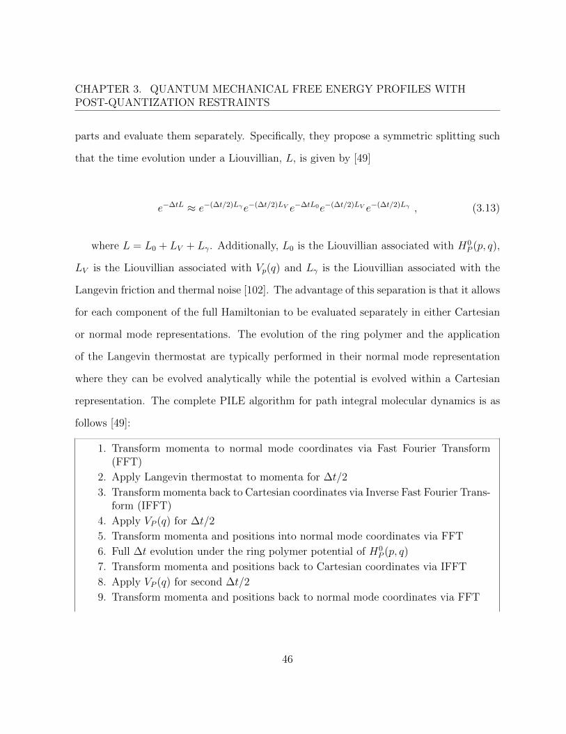
CHAPTER 3. QUANTUM MECHANICAL FREE ENERGY PROFILES WITHPOST-QUANTIZATION RESTRAINTS
parts and evaluate them separately. Specifically, they propose a symmetric splitting such
that the time evolution under a Liouvillian, L, is given by [49]
e−∆tL ≈ e−(∆t/2)Lγe−(∆t/2)LV e−∆tL0e−(∆t/2)LV e−(∆t/2)Lγ , (3.13)
where L = L0 + LV + Lγ. Additionally, L0 is the Liouvillian associated with H0P (p, q),
LV is the Liouvillian associated with Vp(q) and Lγ is the Liouvillian associated with the
Langevin friction and thermal noise [102]. The advantage of this separation is that it allows
for each component of the full Hamiltonian to be evaluated separately in either Cartesian
or normal mode representations. The evolution of the ring polymer and the application
of the Langevin thermostat are typically performed in their normal mode representation
where they can be evolved analytically while the potential is evolved within a Cartesian
representation. The complete PILE algorithm for path integral molecular dynamics is as
follows [49]:
1. Transform momenta to normal mode coordinates via Fast Fourier Transform(FFT)
2. Apply Langevin thermostat to momenta for ∆t/2
3. Transform momenta back to Cartesian coordinates via Inverse Fast Fourier Trans-form (IFFT)
4. Apply VP (q) for ∆t/2
5. Transform momenta and positions into normal mode coordinates via FFT
6. Full ∆t evolution under the ring polymer potential of H0P (p, q)
7. Transform momenta and positions back to Cartesian coordinates via IFFT
8. Apply VP (q) for second ∆t/2
9. Transform momenta and positions back to normal mode coordinates via FFT
46

3.1. THEORETICAL DETAILS
10. Apply Langevin thermostat to momenta for second ∆t/2
11. Transform momenta back to Cartesian coordinates via IFFT
There are a number of transformations between coordinate systems within this al-
gorithm but they are efficient to perform through the use of FFTs and they are not a
bottleneck in this integration scheme. It is also important to note that the non-centroid
modes are analytically derived but the centroid mode requires a tunable friction parameter
as input. The optimal friction parameter for the kth mode in this procedure has been
shown to be [49]:
γ(k) =
1/τ0, k = 0
2ωk, k > 0 ,
(3.14)
where ωk = 2ωP sin(kπ/P ) for the kth normal mode and τ0 is an input parameter
representing some time constant for the centroid mode. The choice of τ0 will vary with
simulation parameters and is commonly calculated by studying the decay of the autocorre-
lation function for some centroid property [77]. Efficiently choosing this τ0 parameter will
be discussed in more detail in Sec. 3.1.4 as it can be related to specific umbrella sampling
parameters.
3.1.3 Umbrella sampling [10,11] and WHAM [62]
Importance sampling is sometimes needed within molecular dynamics simulations in order
to explore regions of phase space that may not be explored with direct sampling of a
Boltzmann distribution. These regions of phase space are often difficult to sample due to
47

CHAPTER 3. QUANTUM MECHANICAL FREE ENERGY PROFILES WITHPOST-QUANTIZATION RESTRAINTS
high energy barriers or possible dissociation events. Umbrella sampling provides a means
to sample these difficult regions by introducing a non-physical potential that biases the
simulation towards such regions.
Consider a Lennard-Jones dimer system with a reaction coordinate defined to be the
distance between the individual monomers. The Lennard-Jones dimer may only explore
the minimum of the potential energy landscape if the temperature is low enough and it
will dissociate if the temperature is high enough. Umbrella sampling proposes a solution
to these sampling problems by modifying the potential such that the total potential in a
simulation is
Vtotal(q, ξw) = V (q) + Vbias(q, ξw) , (3.15)
where V (q) is the physical potential of the system and Vbias(q, ξw) is some biasing
potential centred around the reaction coordinate at ξw. A typical form for the biasing
potential is
Vbias(q, ξw) =1
2kw (ξ(q)− ξw)2 , (3.16)
where kw is a force constant and ξ(q) is the reaction coordinate at a particular configu-
ration. Complete sampling along the desired portion of the reaction coordinate is achieved
by performing simulations where ξw is varied. Each simulation with a different ξw is com-
monly referred to as an umbrella sampling window where ξw and kw are chosen such that
the distributions of adjacent windows overlap.
48
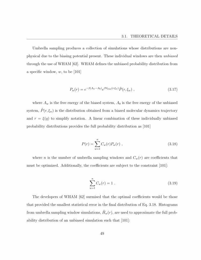
3.1. THEORETICAL DETAILS
Umbrella sampling produces a collection of simulations whose distributions are non-
physical due to the biasing potential present. These individual windows are then unbiased
through the use of WHAM [62]. WHAM defines the unbiased probability distribution from
a specific window, w, to be [101]
Pw(r) = e−β(Aw−A0)eβVbias(r,ξw)P (r, ξw) , (3.17)
where Aw is the free energy of the biased system, A0 is the free energy of the unbiased
system, P (r, ξw) is the distribution obtained from a biased molecular dynamics trajectory
and r = ξ(q) to simplify notation. A linear combination of these individually unbiased
probability distributions provides the full probability distribution as [101]
P (r) =n∑
w=1
Cw(r)Pw(r) , (3.18)
where n is the number of umbrella sampling windows and Cw(r) are coefficients that
must be optimized. Additionally, the coefficients are subject to the constraint [101]:
n∑w=1
Cw(r) = 1 . (3.19)
The developers of WHAM [62] surmised that the optimal coefficients would be those
that provided the smallest statistical error in the final distribution of Eq. 3.18. Histograms
from umbrella sampling window simulations, Hw(r), are used to approximate the full prob-
ability distribution of an unbiased simulation such that [101]:
49

CHAPTER 3. QUANTUM MECHANICAL FREE ENERGY PROFILES WITHPOST-QUANTIZATION RESTRAINTS
P (r, ξw) ≈ 1
nw∆rHw(r) , (3.20)
where nw is the number of samples for window w and ∆r is the width of the bin for the
histogram, Hw(r). The statistical error for a particular simulation is then defined as [101]
σ2w =
εw(r)Hw(r)
nw∆r, (3.21)
where εw(r) describes the deviation between the sampled distribution, P (r, ξw), and
the final distribution, P (r). The statistical error in the unbiased window simulation of
Eq. 3.17 is given by [101]
σ2w = e−2β(Aw−A0)e2βVbias(r,ξw)σ2
w . (3.22)
Combining this statistical error expression with the linear combination of unbiased
distributions of 3.18 yields a final distribution with the statistical error as follows [101]:
σ2 =n∑
w=1
C2w(r)σ2
w . (3.23)
Lagrange multipliers are then used to minimize Eq. 3.23 subject to the constraint that
the coefficients must sum to 1. The final result in the development of WHAM is that the
full unbiased distribution becomes [62,101]
50

3.1. THEORETICAL DETAILS
P (r) =
∑nw=1 nwPw(r)∑n
w=1 nweβ(Aw−A0)e−βVbias(r,ξw)
, (3.24)
where
e−β(Aw−A0) =
∫dq P (r)e−βVbias(r,ξw) . (3.25)
Eq. 3.24 and Eq. 3.25 are the working equations of WHAM that must be solved self-
consistently. It should be noted that there are two important assumptions made in order
to arrive at these two equations. The first assumption is that the deviation function, εw(r),
of Eq. 3.21 is assumed to be the same for all w windows. Secondly, WHAM assumes that
the histograms obtained from simulation, Hw(r), are well approximated by applying the
biasing factor directly to the complete distribution, P (r). Both of these assumptions are
reasonable to make if there is sufficient and equivalent sampling in all of the independent
window simulations [62,101].
The combination of umbrella sampling and WHAM allow for chemical systems to be
simulated with a biasing potential that enhances the sampling of specific regions. Utilizing
these methods requires one to optimize a set of relevant parameters including the number
of umbrella windows (w), as well as the biasing potential force constant (kw) and the
equilibrium value for the biasing potential (ξw) for each window.
51

CHAPTER 3. QUANTUM MECHANICAL FREE ENERGY PROFILES WITHPOST-QUANTIZATION RESTRAINTS
3.1.4 Umbrella sampling with post-quantization restraints
This section details the integration of umbrella sampling techniques within a PIMD and
PILE framework. We begin by considering the biased Hamiltonian,
Hbias = K + V + Vbias , (3.26)
where K is the physical kinetic operator, V is the physical potential operator and Vbias
is the biasing potential operator used in umbrella sampling to explore a specific region of
phase space. Following the derivation presented in Sec. 3.1.1 yields an analogous form of
the partition function for this Hamiltonian:
Zbias = limP→∞
∫dq1 . . . dqP
P∏j=1
ρbiasτ (qj, qj+1) , (3.27)
where the symmetric Trotter type propagator for the biased partition function is given
by
ρbiasτ (qj, qj+1) ≈ e−
τ2
(V (qj)+Vbias(qj))ρ0(qj, qj+1)e−τ2
(V (qj+1)+Vbias(qj+1)) , (3.28)
and ρ0(qj, qj+1) = 〈qj|e−τK |qj+1〉 from Eq. 3.9. Such a partition function is fully imple-
mentable within PIMD simulations utilizing the PILE thermostat for molecular systems.
However, it quickly becomes unrealistic to unbias the umbrella sampling simulations with
WHAM as the Trotter factorization yields P separate biasing potentials. Utilizing WHAM
to unbias a few biasing potentials is possible [103] but hundreds of biasing potentials may
52

3.1. THEORETICAL DETAILS
be needed in order to achieve full convergence of the path integral and this introduces
numerical instability issues within WHAM.
The issue of P biasing potential terms may be eliminated by considering an alternative
form of the partition function [12]:
ZPQR = Tr[e−β(K+V )e−βVbias
](3.29)
= limP→∞
∫dq1 . . . dqP e
−βVbias(q1)
P∏j=1
ρτ (qj, qj+1) , (3.30)
where ρτ (qj, qj+1) is the high temperature density matrix of the unbiased system. This
partition function is subscripted with Post-Quantization Restraint (PQR) due to the fact
that it does not contain a biasing operator like Eq. 3.27. Instead, this partition function
utilizes a classical restraint after quantization to the path integral representation. The
addition of the restraint on a single bead breaks the symmetry of the path integral and only
allows for the data of the biased bead to be gleaned from simulations. This PQR treatment
parallels the post-quantization constraint methodology that was investigated to validate
the use of classical constraint techniques with path integrals [104, 105]. Furthermore, the
attraction of Eq. 3.30 is that the PIMD simulation only needs a biasing potential applied
to a single bead whereas 3.27 required a biasing potential for each bead. Consequently,
WHAM only needs to unbias a single restraint as opposed to P restraints. It should be
noted that the biasing exponential is not divided by P like it is for ρτ (qj, qj+1) and some
PIMD implementations automatically divide the biasing potential by P unless explicitly
53

CHAPTER 3. QUANTUM MECHANICAL FREE ENERGY PROFILES WITHPOST-QUANTIZATION RESTRAINTS
noted.
A common form for the umbrella sampling biasing potential is given by
Vbias(q) =1
2kw (ξ(q)− ξw)2 , (3.31)
where kw is the force constant for window w, ξ(q) is the reaction coordinate as a
function of the configuration and ξw is the equilibrium position of the reaction coordinate
for window w. A number of PIMD simulation windows will need to be executed in order to
study the full path of the reaction coordinate of interest. Every new combination of beads,
simulation temperature, kw and ξw requires a new PIMD simulation and also possesses
a specific Langevin friction parameter that is optimal within the PILE framework. As
discussed in Sec. 3.1.2, the optimal centroid friction parameter is typically determined by
studying the autocorrelation function of some centroid property for a particular simulation.
Ref. [12] proposes that an optimal centroid friction parameter for a simulation window
may be described as
γ0w = 2ωw (3.32)
=
√kwµ, (3.33)
where ωw is the frequency associated with the umbrella sampling biasing potential and
µ is the reduced mass. This form of γ0w is analogous to the higher order modes used within
the PILE thermostat and assumes that the umbrella sampling biasing potential is the
54

3.2. COMPUTATIONAL DETAILS AND RESULTS
dominant portion of the forcefield. It is important to note that the choice of γ0w influences
the rate at which uncorrelated samples will be obtained from simulation. The assumption
of Eq. 3.33 will be analyzed in detail in the following section to determine its efficacy within
umbrella sampling simulations with PQR.
3.2 Computational details and results
This section details how simulations were developed and lists all of the various parameters.
All the simulations performed in this section were done using MMTK [76] unless otherwise
stated. The section begins by discussing the optimal choice of γ0w based upon umbrella
sampling parameters. A Lennard-Jones test system is then used to develop a complete
prescription for accurately obtaining free energy profiles in conjunction with WHAM and
PIMD. Finally, the proposed methodology is tested using a variety of water models for the
water dimer system and computational results are compared against existing simulation
and experimental data.
3.2.1 Optimization of Langevin friction parameter
The Langevin friction parameter, γ0w, is required to thermostat the simulation within the
PILE [49] implementation and the optimal γ0w results in a simulation where uncorrelated
samples are obtained more rapidly. It was proposed in Eq. 3.33 that the optimal γ0w should
be twice the frequency of the harmonic biasing potential used in simulation. In order to
validate this assumption, a number of PIMD simulations with 32 path integral beads were
55

CHAPTER 3. QUANTUM MECHANICAL FREE ENERGY PROFILES WITHPOST-QUANTIZATION RESTRAINTS
performed with a water dimer system using the q-SPC/Fw and Quantum Transferable
Intermolecular Potential with 4 Points Flexible (q-TIP4P/F) water models at 100, 200
and 300 K. The γ0w parameter of the PILE thermostat was varied by orders of magnitude
and the centre of mass distance between the water molecules was outputted for analysis.
An autocorrelation function of the centre of mass distance was created and the decay of
the autocorrelation function dictates the length of time between uncorrelated samples.
Additionally, these simulations utilized kw = 1000 kJ mol−1 nm−2 and ξw = 3, 5, 8 A for
umbrella sampling biasing potentials that were applied to an individual path integral bead.
Finally, the results of these PIMD simulations are presented in Fig. 3.2.
The choice of kw = 1000 kJ mol−1 nm−2 suggests that the optimal γ0w should be 20 ps−1
based on Eq. 3.33. It is observed from Fig. 3.2 that 20 ps−1 does indeed provide a practical
decorrelation time and that the decorrelation time is minimally affected by changes of γ0w
by an order of magnitude in either direction. Consequently, the remaining simulations
performed in this chapter with kw = 1000 kJ mol−1 nm−2 utilize γ0w = 20 ps−1. It is
important to remember that these simulations were performed using only a single biasing
potential on an individual path integral bead as prescribed within Eq. 3.30. A similar
analysis utilizing P biasing potentials revealed that the choice of γ0w was not as stable in
determining the decorrelation time but 20 ps−1 provided a reasonable first guess.
3.2.2 Benchmarking example with Ar2 and Ne2
Lennard-Jones systems are a useful benchmark in validating new theoretical methods due
to the fact that they are often able to be solved exactly. The standard Lennard-Jones
56

3.2. COMPUTATIONAL DETAILS AND RESULTS
10
100 100K
q-SPC/Fw
100K
q-TIP4P/F
10
100 200K 200K
-2 -1 0 1 2 3
10
100 300K
-2 -1 0 1 2 3
300K
log10(γ0w / ps−1)
τ 0 / fs
3 Å 5 Å 8 Å
Figure 3.2: “Optimization of γ0w. 32 bead path integral simulations were performed for
q-SPC/Fw and q-TIP4P/F at 100, 200, and 300 K at separation distances of 3, 5, and 8A. The choice of γ0
w was varied by orders of magnitude, and the decay of autocorrelationfunction for the centre of mass distance was computed and averaged over 100 individualruns with standard errors.” Ref. [12]
57

CHAPTER 3. QUANTUM MECHANICAL FREE ENERGY PROFILES WITHPOST-QUANTIZATION RESTRAINTS
potential is
VLJ(r) = 4ε
[(σr
)12
−(σr
)6], (3.34)
where ε is the depth of the potential well and σ is the distance where the potential is
exactly zero. Each atom has its own Lennard-Jones parameters and the values used for
the argon and neon dimers are summarized in Table 3.1.
Atom Mass / amu ε / kJ mol−1 σ / ANe 39.948 0.997 3.4Ar 20.180 0.306 2.789
Table 3.1: Lennard-Jones parameters for argon and neon.
The motivation for the study of these Lennard-Jones dimers is that they are described
by a single dimensional radial potential. A one-dimensional potential can be exactly evalu-
ated with discretized path integrals using matrix multiplication up to the systematic error
of the Trotter approximation [106]. The methodology of Thirumalai et al. [106] will be
used as our gold standard for the analysis of these Lennard-Jones systems but will not be
practical for higher dimensional problems such as the water dimer system.
Ref. [106] begins by defining the high temperature density matrix from Eq. 3.6 for a
Lennard-Jones dimer as [106]
ρlτ (r, r′) = e−(τ/2)Veff(r)ρfree
τ (r, r′)e−(τ/2)Veff(r′) , (3.35)
where ρfreeτ is the free propagator and Veff is the effective potential that includes the rota-
58

3.2. COMPUTATIONAL DETAILS AND RESULTS
tional energy necessary to describe the partition function in three dimensions. Specifically,
the effective potential is defined as [106]
Veff(r) =l(l + 1)~2
2µr2+ VLJ(r) , (3.36)
where l is the rotational energy level. As before, r is the reaction coordinate defined
as a function of the system configuration such that r = ξ(q). Additionally, they derive the
free propagator for this application to be [106]
ρfreeτ (r, r′) =
[ µ
2π~2τ
]12[e−
µ
2~2τ(r−r′)2
− e−µ
2~2τ(r+r′)2
]. (3.37)
Ref. [106] suggests that performing the matrix multiplication of Eq. 3.35 with itself
produces a new density matrix that is at a temperature of 2τ . This can be effectively
represented by
ρl2τ (r, r′) =
∫ ∞0
dr′′ ρlτ (r, r′′)ρlτ (r
′′, r′) , (3.38)
where r′′ is just an integration variable. Continuing this process for P iterations even-
tually yields the full density matrix at a temperature of β = Pτ for each l. This density
matrix can then be used to evaluate the partition function and free energies of the system
directly.
The exact matrix multiplication results and various molecular dynamics results for the
Lennard-Jones dimers at low temperatures are presented in Fig. 3.3. Classical results are
59

CHAPTER 3. QUANTUM MECHANICAL FREE ENERGY PROFILES WITHPOST-QUANTIZATION RESTRAINTS
realized in both the matrix multiplication and PIMD simulations when P is set to 1. The
results of Fig. 3.3 demonstrate that the classical matrix multiplication code is effectively
reproduced by the classical umbrella sampling code as expected. Quantum umbrella sam-
pling was performed with 512 path integral beads where either a single biasing potential
(R=1) or 512 biasing potentials (R=512) were utilized within simulation. The centre of
mass distance between the atoms was outputted during the course of the simulation and in-
putted into the WHAM implementation of Grossfield [107]. Only the distances associated
with the single biasing potential bead of USP=512,R=1 were used by WHAM while all bead
distances were used in USP=512,R=512 and WHAM. For simplicity, WHAM treated these
512 biasing potentials as if they were a single biasing potential to eliminate the need of a
512-dimensional WHAM. Notably, only the results for 512 bead results are presented here
but other values of P were evaluated in the matrix multiplication calculation. It would
be possible to study the convergence of τ = β/P → 0 for the biased simulations but 512
beads was sufficiently converged for the purpose of this study.
The results of Fig. 3.3 illustrate that only USP=512,R=1 provides an exact agreement
with the matrix multiplication code with the equivalent number of beads. Additionally,
the ‘Monomer’ dataset was obtained using the methodology prescribed to calculate the
second virial coefficient by the developers of the Many Body - polarizable (MB-pol) poten-
tial [44]. For the Monomer dataset, PIMD simulations of both argon and neon monomers
were performed to obtain thermally distributed configurations. These monomer path con-
figurations were then used to provide random monomer orientations at a specific dimer
separation distance in a Monte Carlo algorithm [44]. These results are introduced here
as they are useful when discussing the results in the water dimer simulations where this
60

3.2. COMPUTATIONAL DETAILS AND RESULTS
method captures the quantum mechanics of the water monomers and the temperatures are
higher. In this Lennard-Jones case, the Monomer dataset simply reduces to the classical
umbrella sampling and matrix multiplication results.
The free energy profiles for the Lennard-Jones dimers were then used to calculate
the second virial coefficients and free energy differences using the methods described in
Sec. 3.2.3.1 and Sec. 3.2.3.2 respectively. Classically, the free energy difference at zero
temperature is simply the well depth, ε, while the quantum free energy difference, D0,
was obtained through exact diagonalization of the Lennard-Jones Hamiltonian. Matrix
multiplication calculations were performed at 1 K classically and utilizing 512 path integral
beads to determine the free energy differences as ∆Aexactc and ∆Aexact
q respectively. The
umbrella sampling simulations were performed with either 1 biasing potential or 512 biasing
potentials to determine their free energy differences as ∆AR=1P=512 and ∆AR=512
P=512. These free
energy differences are collected in Table 3.2 for all of these calculation techniques. The
exact matrix multiplication codes reproduce the expected ε value classically and approach
the correct D0 value with 512 beads. Additionally, the ∆AR=1P=512 simulations are also within
the error of the exact multiplication codes while the ∆AR=512P=512 simulations are not. A larger
number of path integral beads would be required for both Ar2 and Ne2 in order for the
matrix multiplication and umbrella sampling codes to converge to the exact D0 obtained
from exact diagonalization at these temperatures.
In summation, the single umbrella sampling biasing potential successfully captures the
behavior of the exact matrix multiplication codes while the P biasing potential umbrella
sampling simulations do not. The rest of this chapter will recognize this and only results
from simulations with a single biasing potential will be presented.
61

CHAPTER 3. QUANTUM MECHANICAL FREE ENERGY PROFILES WITHPOST-QUANTIZATION RESTRAINTS
−1.0
−0.8
−0.6
−0.4
−0.2
0.0
Ar2 - 2.5K
−1.0
−0.8
−0.6
−0.4
−0.2
0.0
Ar2 - 5.0K
2 4 6 8 10−0.30
−0.25
−0.20
−0.15
−0.10
−0.05
0.00
Ne2 - 2.5K
2 4 6 8 10−0.30
−0.25
−0.20
−0.15
−0.10
−0.05
0.00
Ne2 - 5.0K
Dista ce / Å
Free E ergy Profile / kJ mol
−1
ExactcExactq
USP=1,R=1USP=512,R=1
USP=512,R=512Mo omer
Figure 3.3: “Free energy profiles of Ar2 and Ne2 at 2.5 and 5 K using classical and quantumtreatments. The exact data was obtained from matrix multiplication; US data was obtainedusing P beads and R biasing potentials; monomer data was calculated from path integralmonomer simulations.” Ref. [12]
62

3.2. COMPUTATIONAL DETAILS AND RESULTS
System ε D0 ∆Aexactc ∆Aexact
q ∆AR=1P=512 ∆AR=512
P=512
Ar2 -0.998 -0.847 -0.92 -0.80 -0.79(1) -0.65(1)Ne2 -0.306 -0.177 -0.23 -0.14 -0.16(1) -0.10(1)
Table 3.2: ∆A values for Ar2 and Ne2 in kJ/mol at 1K obtained utilizing the methodsdescribed in Section 3.2.3.2. D0 is the dissociation energy and ε is the depth of the Lennard-Jones potential in kJ/mol.
3.2.3 Water dimer results
The ideal forcefield for a molecular dynamics trajectory would be one that is calculated from
an exact electronic structure method at each time step. This type of calculation requires
far too much computational time in order for molecular dynamics simulations to remain
practical. Simpler forcefields are often derived from such electronic structure calculations or
are parameterized within a model to reproduce some known computational or experimental
result. Moreover, water is a very well-studied molecule and there are numerous available
forcefields that have been designed for a variety of situations and needs.
The forcefields that are initially studied here are the q-SPC/Fw [34] and q-TIP4P/F [36]
water models. These forcefield models have been parameterized with path integral simu-
lations in mind such that they will not double count the quantum effects that a non-path
integral forcefield may include in their parameterization. The intermolecular interactions
for the q-SPC/Fw and q-TIP4P/F forcefields are defined as [32,36]
Vinter =∑i
∑j>i
{4ε
[(σ
rij
)12
−(σ
rij
)6]
+∑m∈i
∑n∈j
qmqnrmn
}, (3.39)
where rij is the separation between oxygen atoms and rmn is the separation between
63

CHAPTER 3. QUANTUM MECHANICAL FREE ENERGY PROFILES WITHPOST-QUANTIZATION RESTRAINTS
virtual partial charges in molecules specified by their oxygens i and j. In this expression,
two positive charges of qM/2 are placed on each hydrogen atom and a negative charge of
qM is placed at [32,36]
rM = γrO + (1− γ)(rH1 + rH2)/2 , (3.40)
where γ is the fraction parameter that can move the negative charge off of the oxygen
directly. The parameters for both the q-SPC/Fw and q-TIP4P/F models are provided in
Table 3.3. For the 3-site water model, q-SPC/Fw, γ = 1 and the negative charge is directly
on the oxygen atoms. For the 4-site water model, q-TIP4P/F , γ 6= 1 and the negative
charge is no longer on the oxygen directly.
The intramolecular portion of the forcefields is described by [36]
Vintra =∑i
[VOH(ri1) + VOH(ri2) +
1
2kθ(θi − θeq)2
], (3.41)
where VOH(ri1) describes the O-H bond distance interaction, kθ is the force constant for
the harmonic angle stretch, θi is the instantaneous bond angle for molecule i and θeq is the
equilibrium bond angle. For q-SPC/Fw, the bond distance expression is [34]
Vq-SPC/Fw
OH (r) =1
2kr(r − req)2 , (3.42)
where kr is the force constant for the harmonic stretch and req is the equilibrium bond
distance. The q-TIP4P/F forcefield utilizes an expansion of a Morse potential such that
64

3.2. COMPUTATIONAL DETAILS AND RESULTS
q-SPC/Fw q-TIP4P/F
kr / kJ mol−1 A−2 4431.533 N/Areq / A 1.0000 0.9419
Dr / kJ mol−1 N/A 485.72αr / A−1 N/A 2.287
kθ / kJ mol−1 A−2 317.57 367.56θeq / degrees 112.0 107.4ε / kJ mol−1 0.6502 0.7749
σ / A 3.1655 3.1589qM / |e| 0.84 1.1128
γ 1.00 0.73612
Table 3.3: Parameters for the q-TIP4P/F [36] and q-SPC/Fw [34] water models.
the bond interaction becomes [36]
Vq-TIP4P/F
OH (r) = Dr
[α2r(r − req)2 − α3
r(r − req)3 +7
12α4r(r − req)4
], (3.43)
where Dr and αr are the standard Morse potential parameters. A detailed parameter
list for all of these forcefield expressions is provided in Table 3.3.
The q-SPC/Fw and q-TIP4P/F water models were developed to study liquid water
at ambient temperatures within PIMD and not for studying a single water dimer over a
broad range of temperatures. Accurately obtaining properties for smaller water clusters
at lower temperatures is made possible through the use of a many-body forcefield such
as CC-pol [42], WHBB [108], HBB2-pol [43] or MB-pol [44–47]. This work will utilize
the MB-pol potential in order to make accurate comparisons to physical experimental
data at low and high temperatures. The MB-pol potential was built upon the results
65

CHAPTER 3. QUANTUM MECHANICAL FREE ENERGY PROFILES WITHPOST-QUANTIZATION RESTRAINTS
of fitting 40,000 water dimer energies from Coupled Cluster Singles and Doubles with
perturbative Triples (CCSD(T)) calculations with machine learning techniques [44]. This
forcefield has been shown to accurately reproduce experimental vibration-rotation spectra
and the second virial coefficient of the water dimer [44]. One potential drawback is the
computational cost associated with MB-pol as it requires about 6-8x the computational
resources in comparison to the much simpler q-SPC/Fw model.
The path integral umbrella sampling simulations were performed using γ0w = 20 ps−1 for
the q-SPC/Fw, q-TIP4P/F and MB-pol water models from 10 - 300 K. PIMD simulations
were equilibrated for 1 ns before beginning a data collection period of 10 ns with a time
step of 0.1 fs. The centre of mass distance between the water molecules was outputted from
simulation for the bead which was modified to include the single umbrella sampling biasing
potential. Free energy profiles were then generated by the WHAM implementation of
Grossfield [107]. Finally, it should be noted that a correction was added to the output of the
WHAM code to account for the Jacobian transformation from Cartesian coordinates to the
radial separation distance between the centre of mass of the water monomers. Specifically,
the Helmholtz free energy as a function of the reaction coordinate, r = ξ(q), is given
by [109,110]
A(r) = −kBT lnP (r) + 2kBT ln r + constant , (3.44)
where P (r) is the probability distribution as a function of the reaction coordinate. This
probability distribution is obtained from the output of the WHAM implementation [107]
of Eq. 3.24 and the second term in Eq. 3.44 is the Jacobian correction. Notably, this
66

3.2. COMPUTATIONAL DETAILS AND RESULTS
formulation is only accurate up to some integration constant that effectively sets the zero
of energy in this scenario. The results of these path integral umbrella sampling simulations
are presented in Figs. 3.4 - 3.9 for the q-SPC/Fw, q-TIP4P/F and MB-pol models over
the complete range of temperatures. Additionally, classical umbrella sampling simulations,
classical rigid monomer simulations and the quantum monomer technique of Ref. [44] are
presented in these figures.
Qualitatively, q-SPC/Fw, q-TIP4P/F and MB-pol all appear similar to one another
in these results. However, there are quantitative differences between the various methods
used to calculate the free energy profiles. It is important to remember that Sec. 3.2.2
demonstrated that the single biasing potential in conjunction with PIMD and WHAM
was the only method that provides the exact quantum result at low temperature. At
temperatures above 100 K, the quantum Monomer data agrees well with the quantum
umbrella sampling data and the classical rigid monomer simulations fall in between the
classical and quantum methodologies. It is at the lower temperatures where the rigid
monomer implementation does increasingly more poor and the quantum monomer method
diverges from the quantum umbrella sampling simulations. The attractive part of the free
energy profile becomes increasingly wide at the 10 and 25 K simulations for the quantum
umbrella sampling just as it did in the Lennard-Jones system. However, the quantum
monomer method fails to capture this broadening due to the fact that only the monomers
are treated with path integrals while the actual reaction coordinate itself is treated via
a classical Monte Carlo code [44]. This quantum monomer prescription works fairly well
down to 100 K but is insufficient for the simulations at 50 K and below. It is also important
to note that a smaller separation between umbrella sampling windows was required in order
67

CHAPTER 3. QUANTUM MECHANICAL FREE ENERGY PROFILES WITHPOST-QUANTIZATION RESTRAINTS
−30
−25
−20
−15
−10
−5
0
10.0K−25
−20
−15
−10
−5
0
25.0K
2 4 6 8 10
−25
−20
−15
−10
−5
0
50.0K2 4 6 8 10
−25
−20
−15
−10
−5
0
100.0K
Distance / Å
Free Energy Profile / kJ mol−1
MonomerP=1MonomerP=512
USP=1USP=512
Rigid MC
Figure 3.4: Free energy profiles as a function of the centre of mass separation distance forthe q-SPC/Fw water dimer from classical flexible, classical rigid and quantum simulationsat 10, 25, 50 and 100K. The ‘Monomer’ results were obtained following the procedureof Ref. [44] and the ‘US’ results were obtained from the procedure described within thischapter.
68
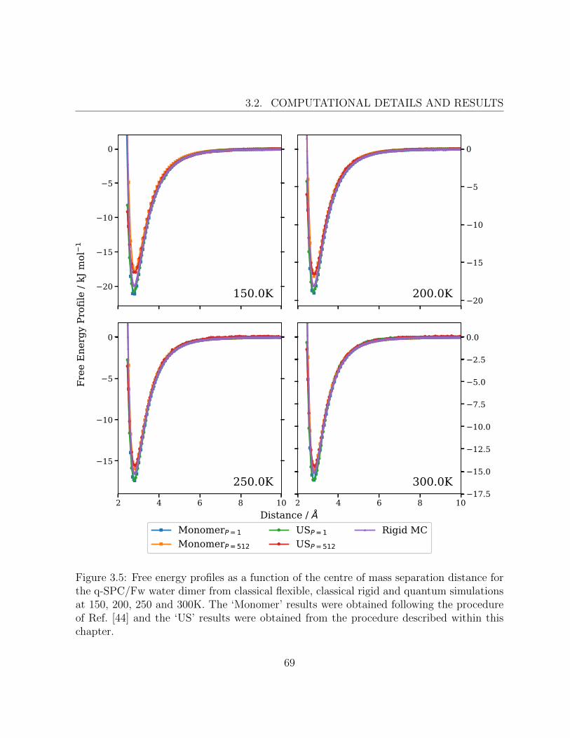
3.2. COMPUTATIONAL DETAILS AND RESULTS
−20
−15
−10
−5
0
150.0K−20
−15
−10
−5
0
200.0K
2 4 6 8 10
−15
−10
−5
0
250.0K2 4 6 8 10
−17.5
−15.0
−12.5
−10.0
−7.5
−5.0
−2.5
0.0
300.0K
Distance / Å
Free Energy Profile / kJ ol−1
Mono erP=1Mono erP=512
USP=1USP=512
Rigid MC
Figure 3.5: Free energy profiles as a function of the centre of mass separation distance forthe q-SPC/Fw water dimer from classical flexible, classical rigid and quantum simulationsat 150, 200, 250 and 300K. The ‘Monomer’ results were obtained following the procedureof Ref. [44] and the ‘US’ results were obtained from the procedure described within thischapter.
69

CHAPTER 3. QUANTUM MECHANICAL FREE ENERGY PROFILES WITHPOST-QUANTIZATION RESTRAINTS
−25
−20
−15
−10
−5
0
10.0K −25
−20
−15
−10
−5
0
25.0K
2 4 6 8 10−25
−20
−15
−10
−5
0
50.0K2 4 6 8 10
−20
−15
−10
−5
0
100.0K
Distance / Å
Free Ene
rgy Pr file
/ kJ m
l−1
M n merP=1M n merP=512
USP=1USP=512
Rigid MC
Figure 3.6: Free energy profiles as a function of the centre of mass separation distance forthe q-TIP4P/F water dimer from classical flexible, classical rigid and quantum simulationsat 10, 25, 50 and 100K. The ‘Monomer’ results were obtained following the procedureof Ref. [44] and the ‘US’ results were obtained from the procedure described within thischapter.
70

3.2. COMPUTATIONAL DETAILS AND RESULTS
−20.0
−17.5
−15.0
−12.5
−10.0
−7.5
−5.0
−2.5
0.0
150.0K −17.5
−15.0
−12.5
−10.0
−7.5
−5.0
−2.5
0.0
200.0K
2 4 6 8 10
−15.0
−12.5
−10.0
−7.5
−5.0
−2.5
0.0
250.0K2 4 6 8 10
−15.0
−12.5
−10.0
−7.5
−5.0
−2.5
0.0
300.0K
Distance / Å
Free Energy Profile / kJ ol−1
Mono erP=1Mono erP=512
USP=1USP=512
Rigid MC
Figure 3.7: Free energy profiles as a function of the centre of mass separation distance forthe q-TIP4P/F water dimer from classical flexible, classical rigid and quantum simulationsat 150, 200, 250 and 300K. The ‘Monomer’ results were obtained following the procedureof Ref. [44] and the ‘US’ results were obtained from the procedure described within thischapter.
71

CHAPTER 3. QUANTUM MECHANICAL FREE ENERGY PROFILES WITHPOST-QUANTIZATION RESTRAINTS
−20
−15
−10
−5
0
10.0K−20.0
−17.5
−15.0
−12.5
−10.0
−7.5
−5.0
−2.5
0.0
25.0K
2 4 6 8 10
−15
−10
−5
0
50.0K2 4 6 8 10
−15.0
−12.5
−10.0
−7.5
−5.0
−2.5
0.0
100.0K
Distance / Å
Free Energy Profile / kJ mol−1
MonomerP=1MonomerP=512
USP=1USP=512
Rigid MC
Figure 3.8: Free energy profiles as a function of the centre of mass separation distance forthe MB-pol water dimer from classical flexible, classical rigid and quantum simulationsat 10, 25, 50 and 100K. The ‘Monomer’ results were obtained following the procedureof Ref. [44] and the ‘US’ results were obtained from the procedure described within thischapter.
72

3.2. COMPUTATIONAL DETAILS AND RESULTS
−14
−12
−10
−8
−6
−4
−2
0
150.0K −12
−10
−8
−6
−4
−2
0
200.0K
2 4 6 8 10
−10
−8
−6
−4
−2
0
250.0K2 4 6 8 10
−10
−8
−6
−4
−2
0
300.0K
Distance / Å
Free Energy Profile / kJ mol−1
MonomerP=1MonomerP=512
USP=1USP=512
Rigid MC
Figure 3.9: Free energy profiles as a function of the centre of mass separation distance forthe MB-pol water dimer from classical flexible, classical rigid and quantum simulationsat 150, 20, 250 and 300K. The ‘Monomer’ results were obtained following the procedureof Ref. [44] and the ‘US’ results were obtained from the procedure described within thischapter.
73

CHAPTER 3. QUANTUM MECHANICAL FREE ENERGY PROFILES WITHPOST-QUANTIZATION RESTRAINTS
to achieve overlap between adjacent window distributions at 10 K. Specifically, the higher
temperature simulations varied ξw from 2 to 10 A in 0.5 A increments while 10 K required
0.1 A increments with the same biasing potential force constant.
These free energy profiles provide a qualitative and quantitative description of the water
dimer system. However, the free energy profiles must be converted into another quantity
in order for comparisons to other computational and experimental data to be possible.
3.2.3.1 Second virial coefficients
Virial coefficients come from the many-body expansion of the ideal gas law to provide
information about the interactions present within a system. Specifically, the second virial
coefficient represents the interactions between pairs of molecules within the system. A
typical expression for the second virial coefficient in radial coordinates is given by
B2(T ) = −2π
∫dr r2
(e−βAξ(r) − 1
), (3.45)
where Aξ(r) is the free energy profile as before. The portion of Eq. 3.45 within the
parentheses is known as the Mayer function and it is designed to go to zero at long range
such that the integral in this equation converges.
The free energy profiles of MB-pol of the previous section were integrated according to
Eq. 3.45 and the second virial coefficients are displayed in Fig. 3.10. At this point, only the
MB-pol second virial coefficients are displayed as the q-SPC/Fw and q-TIP4P/F models
do not even remotely represent the experimental data for the second virial coefficient.
74

3.2. COMPUTATIONAL DETAILS AND RESULTS
Fig. 3.10 demonstrates that all of the classical and quantum methodologies discussed thus
far do a reasonable job in determining the second virial coefficient in the temperature range
at which the experiments can be performed.
3.2.3.2 Free energy differences
In the zero temperature limit, the free energy difference collapses to the dissociation energy
of the water dimer and the dissociation energy can be determined experimentally [13]. In
order to calculate the free energy difference, consider an alternative definition for the second
virial coefficient of the previous section [113]:
B2(T ) = V
(1
2− ZdZ2m
), (3.46)
where Zd is the dimer partition function, Zm is the monomer partition function and V
is the volume describing the system. The Helmholtz free energy difference can be shown
to be
∆A = Ad − 2Am (3.47)
= −kBT lnZd − 2(−kBT lnZm) (3.48)
= −kBT lnZdZ2m
, (3.49)
where Ad and Am are the Helmholtz free energy of the dimer and monomer respec-
tively. Combining Eq. 3.46 with Eq. 3.49 yields the following expression for the free energy
75

CHAPTER 3. QUANTUM MECHANICAL FREE ENERGY PROFILES WITHPOST-QUANTIZATION RESTRAINTS
250 300 350 400 450 500Temperature / K
−4000
−3500
−3000
−2500
−2000
−1500
−1000
−500
0
B2 / cm−3
Classical USQuantum USRigid MCClassical MonomerQuantum MonomerHarvey and Lemmona
Duska and Hrubyb
Figure 3.10: “Second virial coefficients for MB-pol from classical flexible, classical rigidand quantum simulations as well as the experimental data of a and b from Ref. [111] andRef. [112], respectively.” Ref. [12]
76

3.2. COMPUTATIONAL DETAILS AND RESULTS
difference:
∆A = −kBT ln
(1
2− B2(T )
V
). (3.50)
The second virial coefficients of Fig. 3.10 are now able to be used to calculate the free
energy differences via Eq. 3.50. These free energy differences are plotted in Fig. 3.11 for the
MB-pol potential with the classical, classical rigid and quantum methodologies. Addition-
ally, the change in internal energy, ∆U , and the Harmonic Oscillator-Rigid Rotor (HO-RR)
approximation were included in the plot. The zero temperature classical limit, V mincl is sim-
ply the minimum of the MB-pol potential and DHO0 is the dissociation energy calculated
within the HO-RR approximation. Furthermore, a velocity map imaging experiment has
obtained a dissociation energy of 13.2 ± 0.12 kJ/mol for the water dimer [13]. It should
also be noted that the dissociation energy for the water dimer with the MB-pol potential
has recently been determined accurately via diffusion Monte Carlo [114] and Path Integral
Ground State (PIGS) [82].
The results in Fig. 3.11 are only presented down to 25 K due to the fact that the
Mayer function in Eq. 3.45 no longer goes to 0 at long distance and the second virial
coefficient goes to negative infinity. This behaviour arises at low temperature due to the
fact that bound states dominate the partition function compared to the continuum states.
At these temperatures, distance becomes an ill-defined reaction coordinate and the energy
differences between dimers and monomers becomes more practical. In order to obtain
reasonable ground state convergence, the difference between the HO-RR approximation at
25 K and its ground state limit was stitched onto the end of the 25 K quantum umbrella
77

CHAPTER 3. QUANTUM MECHANICAL FREE ENERGY PROFILES WITHPOST-QUANTIZATION RESTRAINTS
0.00 0.01 0.02 0.03 0.04 0.05T−1 / K−1
−20
−15
−10
−5
0
5
ΔA / kJ m
ol−1
Vmincl
DHOΔ
Cla icalRigidQuantumΔUHO-RRExpt.a
Figure 3.11: “∆A was calculated using Eq. 3.50 for MB-pol water dimer. The classicaland quantum data were obtained using umbrella sampling on a single bead with 1 and512 path integral beads, respectively. The rigid data were obtained from Monte Carlosimulations with rigid monomers. Finally, HO-RR refers to the harmonic oscillator-rigidrotor approximation, ∆U refers to the difference in internal energy, and the experimentaldata comes from Ref. [13].” Ref. [12]
78

3.3. CONCLUSIONS
sampling data. This simple approximate extrapolation realizes a free energy difference of
∆A = −12.90 ± 0.05 kJ/mol that is nearly within the experimental error for the quantum
umbrella sampling result.
3.3 Conclusions
This chapter has focused on developing a methodology to accurately determine free energy
differences utilizing the tools of umbrella sampling in conjunction with PIMD. The relevant
portions of the existing PILE and umbrella sampling methodologies are described and key
parameter optimizations for these methods are analyzed. Specifically, the assumption is
made that the optimal Langevin friction parameter of the PILE thermostat can be approxi-
mated by twice the frequency associated with the umbrella sampling biasing potential. The
critical component in the combination of these methods is the application of an umbrella
sampling biasing potential on a single path integral bead. This type of umbrella sampling
restraint is referred to as PQR for post-quantization restraint.
The PQR methodology was validated against a Lennard-Jones benchmark system of
Ar2 and Ne2 for which the exact free energy profiles can be computed. It was observed
that the single bead restraint of PQR exactly reproduces the matrix multiplication results
obtained from the methodology prescribed by Thirumalai et al. [106]. Finally, the free
energy profiles of both Ar2 and Ne2 were utilized to determine the free energy difference
between dimer and monomer utilizing an intermediary calculation of their second virial
coefficients.
79

CHAPTER 3. QUANTUM MECHANICAL FREE ENERGY PROFILES WITHPOST-QUANTIZATION RESTRAINTS
The successful validation of the PQR method on the Lennard-Jones systems allowed
for the use of PQR on the more complicated water dimer system. Free energy profiles were
obtained using the PQR methodology for the q-SPC/Fw, q-TIP4P/F and MB-pol water
models. The q-SPC/Fw and q-TIP4P/F models were initially used to test the efficiency
of the methodology before the more expensive MB-pol model was simulated. In the high
temperature limit, a classical methodology is sufficient to accurately determine the free
energy profiles and second virial coefficients. However, the classical methods lose their
accuracy as the temperature is lowered and classical rigid monomer simulations provide a
cheap approximation to the quantum methods for some intermediary temperatures. The
procedure from Ref. [44] effectively treats the water monomers quantum mechanically and
the reaction coordinate itself classically. This mixed quantum classical treatment provides
reasonable free energy profiles and second virial coefficients over a range of temperatures
but is inadequate as the temperature is lowered below 100 K. As a result, the second virial
coefficients and free energy profiles were only accurately evaluated at low temperature
through the use of the PQR method. Furthermore, extrapolation to the ground state limit
of the ∆A results was performed for the PQR method to yield a ∆A of -12.90± 0.05 kJ/mol
in comparison to the experimental dissociation energy of 13.2 ± 0.12 kJ/mol [13]. The
calculation of the second virial coefficient became increasingly difficult as the temperature
was lowered. This difficulty arises due to the fact that the inter-monomer distance became
an impractical reaction coordinate and the second virial coefficient becomes very large and
negative.
From a practical standpoint, the classical simulation methods are sufficient for the ac-
curate determination of the free energy profiles at high temperatures. Introducing rigid
80

3.3. CONCLUSIONS
monomers within the classical methods provides for accurate results at lower temperatures
and the use of quantum monomer simulations provides accurate results at even lower tem-
peratures. However, the PQR method accurately determines the second virial coefficients
and free energy differences at even lower temperatures. It is important to note that the
HO-RR approximation also works well over a broad portion of this temperature range but
its accuracy would not be able to be quantified without these PQR results. Finally, it
becomes more practical to utilize diffusion Monte Carlo [114] or PIGS [82] to study the
dissociation energy and other properties if you only need to calculate them in the ground
state limit.
81


Chapter 4
Quantum mechanical free energy
profiles from constrained path
integral molecular dynamics
The material covered within this chapter mirrors a lot of the content from Chapter 3
in regards to the calculation of free energies through PIMD simulations. One potential
drawback of the PQR method of Chapter 3 is that the umbrella sampling parameters need
to be chosen properly and this often necessitates some trial and error. For example, the
number of umbrella sampling windows and their associated biasing potentials need to be
carefully chosen to provide sufficient overlap in the distributions of adjacent windows. The
aim for this chapter is to introduce and validate a novel method to calculate the quantum
mechanical free energy without the use of umbrella sampling and the associated unbiasing
83

CHAPTER 4. QUANTUM MECHANICAL FREE ENERGY PROFILES FROMCONSTRAINED PATH INTEGRAL MOLECULAR DYNAMICS
techniques.
The majority of the theoretical development of this method has been derived by Dmitri
Iouchtchenko and the formal details of these derivations will be made available in future
manuscripts [15, 115]. Specifically, these manuscripts formally derive estimators for the
derivative of the free energy with respect to a reaction coordinate on simplified systems
that are subsequently validated against Path Integral Monte Carlo (PIMC) and matrix
multiplication results. Integrating the derivative of the free energy over the reaction co-
ordinate to obtain the free energy itself is analogous to the method of thermodynamic
integration originally proposed by Kirkwood [14].
The goal of this chapter1 is to develop a PIMD framework based upon the estimators
proposed in Ref. [15]. This chapter begins by providing a summary of the relevant com-
ponents and estimators proposed by Iouchtchenko et al. [15] in Sec. 4.1.1. Constraints
within molecular dynamics are discussed in Sec. 4.1.2 before a full implementation within
OpenMM for a constrained PIMD simulation is described in Sec. 4.1.3. Finally, the con-
strained PIMD methodology within OpenMM is validated against a pair of Lennard-Jones
systems in Sec. 4.2 before it is applied to the more complicated water dimer in Sec. 4.3.
The results in 4.3 are then benchmarked against the theoretical results from Chapter 3 for
the q-SPC/Fw, q-TIP4P/F and MB-pol water potentials.
1This material presented in this chapter will be used in another manuscript that is currently in prepa-ration and will be submitted for publication as Ref. [116].
84

4.1. THEORY AND SOFTWARE IMPLEMENTATION
4.1 Theory and software implementation
This section begins by detailing the relevant portions for the derivation of new estimators
for the derivative of the free energy described in Ref. [15]. The resulting estimators for
the derivative of the free energy require a constraint on a single bead of the path integral
within simulation. As a result, this section will also cover the fundamentals of constraints
within molecular dynamics simulations before describing a complete implementation for
constrained PIMD within the OpenMM software package.
4.1.1 Estimators for the derivative of the free energy
The Helmholtz free energy of a system as a function of reaction coordinate, ξ∗, is given by
A(ξ∗) = −kBT lnP (ξ∗) , (4.1)
where P (ξ∗) is the probability distribution evaluated at a specific value of the reaction
coordinate, ξ∗. Within quantum mechanics, the probability distribution may be expressed
as
P (ξ∗) = ρ(ξ∗) = 〈ξ∗|TrX e−βH |ξ∗〉 , (4.2)
where X and ξ are set of coordinates transformed from the standard Cartesian coor-
dinates, q, and TrX e−βH is the reduced density operator. Specifically, ξ is the general
reaction coordinate, ξ∗ is a specific value of the reaction coordinate and X contains the
85

CHAPTER 4. QUANTUM MECHANICAL FREE ENERGY PROFILES FROMCONSTRAINED PATH INTEGRAL MOLECULAR DYNAMICS
rest of the transformation coordinates. The derivative of the free energy with respect to
the reaction coordinate is
A′(ξ∗) =∂
∂ξA(ξ∗) =
∂
∂ξ(−kBT ln ρ(ξ∗)) = −kBT
ρ′(ξ∗)
ρ(ξ∗). (4.3)
The critical component of this theory is the evaluation of A′(ξ∗) from a single PIMD
simulation. An accurate determination of A′(ξ∗) over a sufficiently large range of ξ∗ can
be integrated in order to obtain the complete free energy, A(ξ∗). The derivation for the
estimators begins by considering the density in Eq. 4.3 in Cartesian coordinates,
ρ(ξ∗) =
∫dq δ(ξ(q1)− ξ∗) 〈q|e−βH |q〉 , (4.4)
where ξ(q1) is the reaction coordinate as a function of the current Cartesian coordinates
for the first path integral bead. The remaining component of Eq. 4.3 is the derivative of
the density, ρ′(ξ∗), for which Ref. [15] proposes two methods to obtain this quantity.
The first proposed method initially performs the differentiation of Eq. 4.3 in the oper-
ator representation before the resulting derivative is then discretized into its path integral
representation. Details on this derivation are available in Ref. [15] and the final result is
that the derivative of the density for f degrees of freedom and P beads is given by
86

4.1. THEORY AND SOFTWARE IMPLEMENTATION
ρ′(ξ∗) ≈∫
dq1· · ·∫
dqP δ(ξ(q1)− ξ∗)π(q1, . . . ,qP )×[∂
∂ξln |J(q1)| − β
P
f∑i=1
∂qi(q1)
∂ξ
P∑j=1
∂V (qj)
∂qi
], (4.5)
where J(q1) is the Jacobian associated with the transformation from q1 to {X, ξ} and
π(q1, . . . ,qP ) = 〈q1|e−τH |q2〉 〈q2|e−τH |q3〉 . . . 〈qP |e−τH |q1〉 . (4.6)
Additionally, ∂qi(q1)∂ξ
is the derivative with respect to ξ for bead 1 of the ith degree of
freedom and∂V (qj)
∂qiis the derivative of the potential for bead j with respect to the ith
degree of freedom. It should be noted that Eq. 4.5 becomes exact in the limit of infinite P
and that the delta function in Eq. 4.5 is only applied to the first bead. The derivative of
the free energy is thus obtained by inserting the result of Eq. 4.5 into Eq. 4.3:
A′Est1(ξ∗) = −kBT
⟨∂
∂ξln |J(q1)| − β
P
f∑i=1
∂qi(q1)
∂ξ
P∑j=1
∂V (qj)
∂qi
⟩ξ∗,P
, (4.7)
where the subscripts on the average indicate a constraint at ξ∗ and that P path integral
beads were used in the discretization. The second term in the average of Eq. 4.7 is simply
the average over the path integral of the force along the reaction coordinate evaluated
over all the degrees of freedom. This estimator described by Eq. 4.7 will be referred to as
‘Estimator 1’ or ‘Est1’ throughout the rest of this chapter.
The second proposed method to calculate ρ′(ξ∗) requires one to first discretize the den-
87

CHAPTER 4. QUANTUM MECHANICAL FREE ENERGY PROFILES FROMCONSTRAINED PATH INTEGRAL MOLECULAR DYNAMICS
sity operator and then evaluate the derivative in the path integral representation. Ref. [15]
has shown that the derivative of the density for this method for f degrees of freedom and
P beads is
ρ′(ξ∗) ≈∫
dq1· · ·∫
dqP δ(ξ(q1)− ξ∗)π(q1, . . . ,qP )×[∂
∂ξln |J(q1)| − β
P
∂V (q1)
∂ξ−
f∑i=1
miP
~2β
∂qi(q1)
∂ξ(2qi(q1)− qi(q2)− qi(qP ))
],
(4.8)
As before, Eq. 4.8 becomes exact in the limit of infinite beads and the constraint is
only present on the first path integral bead. Similarly, the derivative of the free energy is
evaluated by inserting Eq. 4.8 into Eq. 4.3:
A′Est2(ξ∗) = −kBT×⟨∂
∂ξln |J(q1)| − β
P
∂V (q1)
∂ξ−
f∑i=1
miP
~2β
∂qi(q1)
∂ξ(2qi(q1)− qi(q2)− qi(qP ))
⟩ξ∗,P
,
(4.9)
where the subscripts on the average again indicate a constraint at ξ∗ and that P path
integral beads were used in the discretization. The form of the estimator in Eq. 4.9 is very
different than the estimator in Eq. 4.7 due to the fact that only the constrained bead and
its direct neighbours are present. This estimator described by Eq. 4.9 will be referred to
88

4.1. THEORY AND SOFTWARE IMPLEMENTATION
as ‘Estimator 2’ or ‘Est2’ throughout the rest of this chapter. In theory, both of these
estimators are exact but in practice, these estimators converge differently with respect to
the numerical sampling and the number of path integral beads [15].
There are a few quantities in these estimators that need to be defined clearly for a
specific reaction coordinate. The reaction coordinate used in the upcoming sections is
the distance between Lennard-Jones atoms or the distance between the oxygens of the
water dimer. Ref. [15] has shown that the Jacobian piece of these estimators for a reaction
coordinate defined as the distance between 2 atoms is given by
∂
∂ξlog |J(q)| = 2
ξ. (4.10)
Additionally, Ref. [15] has shown that the partial derivatives with respect to the reaction
coordinate defined as the distance between 2 atoms are given by
∂q1(qi)
∂ξ=q1(qi)− q2(qi)
2ξ(4.11)
∂q2(qi)
∂ξ= −q1(qi)− q2(qi)
2ξ(4.12)
∂q≥3(qi)
∂ξ= 0 . (4.13)
At this point, both Estimator 1 and Estimator 2 are well defined and ready to be
implemented within a constrained PIMD framework. The key part remaining is the proper
application of the constraint to a single bead within a PIMD simulation.
89
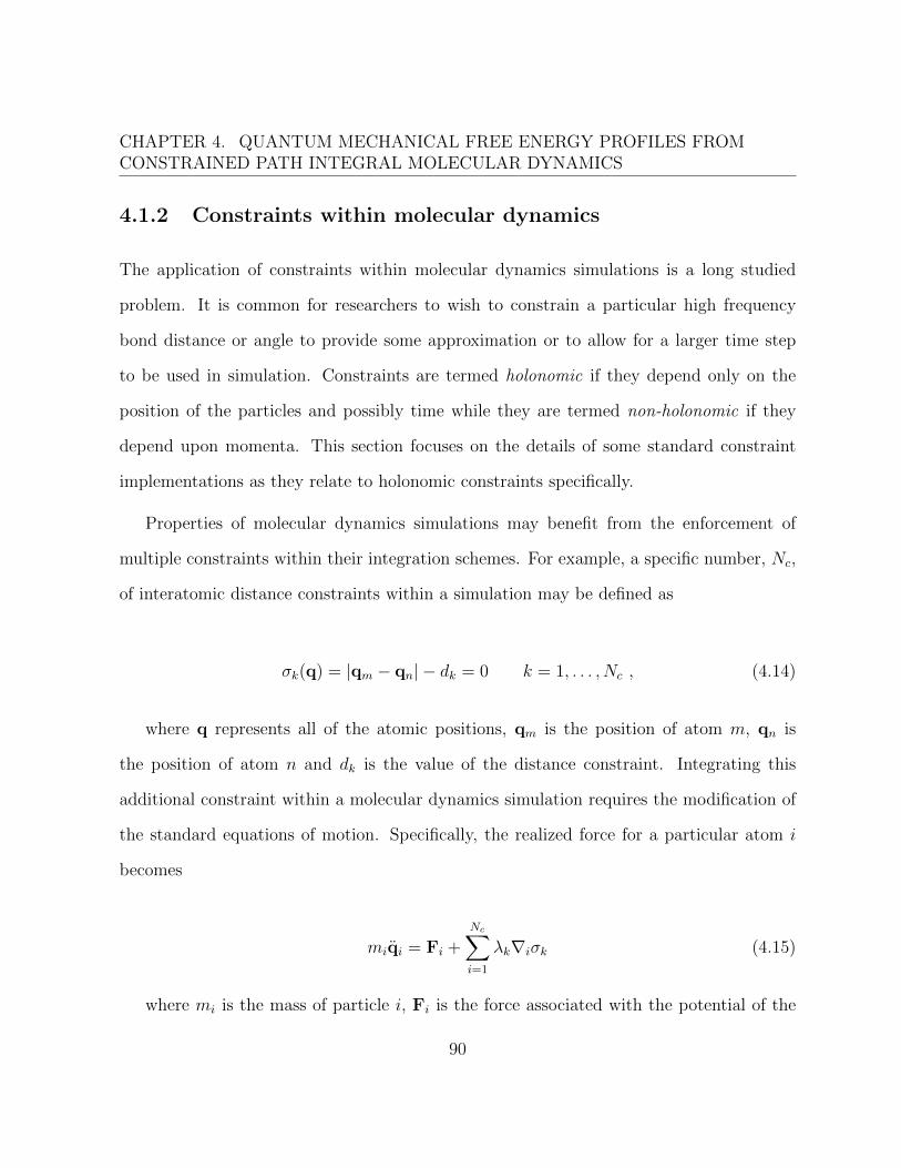
CHAPTER 4. QUANTUM MECHANICAL FREE ENERGY PROFILES FROMCONSTRAINED PATH INTEGRAL MOLECULAR DYNAMICS
4.1.2 Constraints within molecular dynamics
The application of constraints within molecular dynamics simulations is a long studied
problem. It is common for researchers to wish to constrain a particular high frequency
bond distance or angle to provide some approximation or to allow for a larger time step
to be used in simulation. Constraints are termed holonomic if they depend only on the
position of the particles and possibly time while they are termed non-holonomic if they
depend upon momenta. This section focuses on the details of some standard constraint
implementations as they relate to holonomic constraints specifically.
Properties of molecular dynamics simulations may benefit from the enforcement of
multiple constraints within their integration schemes. For example, a specific number, Nc,
of interatomic distance constraints within a simulation may be defined as
σk(q) = |qm − qn| − dk = 0 k = 1, . . . , Nc , (4.14)
where q represents all of the atomic positions, qm is the position of atom m, qn is
the position of atom n and dk is the value of the distance constraint. Integrating this
additional constraint within a molecular dynamics simulation requires the modification of
the standard equations of motion. Specifically, the realized force for a particular atom i
becomes
miqi = Fi +Nc∑i=1
λk∇iσk (4.15)
where mi is the mass of particle i, Fi is the force associated with the potential of the
90

4.1. THEORY AND SOFTWARE IMPLEMENTATION
system for particle i and λk is a set of Lagrange multipliers that are designed to enforce
the constraints. Additionally, the constraints themselves are fixed over the course of the
simulation such that the time derivative of the constraints is zero:
d
dtσk(q) = 0 . (4.16)
One such method that can accurately determine these Lagrange multipliers and enforce
their associated constraints is the SHAKE algorithm [117]. Within the SHAKE algorithm,
a system of linear equations is developed and iteratively solved for at each time step until
the constraint equations are valid. Typically, this is done through the creation and inversion
of a matrix that scales in size with the number of atoms and constraints present in the
system. This prescription works well for small molecules where the small matrices can be
manipulated efficiently but having to evaluate these matrices at each time step quickly
becomes a bottleneck for larger chemical systems and their associated larger matrices.
There are a number of additional constraint methodologies that can efficiently solve
for these Lagrange multipliers [118–120]. The SETTLE algorithm [119] is particularly
useful as it analytically solves for the Lagrange multipliers but it does not scale to more
than 3 constraints. Nevertheless, the SETTLE algorithm is commonly used in simulations
where rigid water molecules are present [119]. A final constraint methodology discussed
here is the Constant Constraint Matrix Approximation (CCMA) algorithm [121] that is
implemented within OpenMM [84]. The CCMA algorithm makes an approximation within
the SHAKE algorithm that the expensive matrix operations required at each time step for
SHAKE only need to be performed at the beginning of a simulation. This approximate
91

CHAPTER 4. QUANTUM MECHANICAL FREE ENERGY PROFILES FROMCONSTRAINED PATH INTEGRAL MOLECULAR DYNAMICS
constraint matrix used within CCMA is dictated by the bond angles present in simulation.
Specifically, the bond angles in the constraint matrix are modified to either represent their
constrained value or their equilibrium value as defined by their harmonic bond angle force.
The authors of CCMA have shown that the CCMA approximation works well for harmonic
forcefields and is far more computationally efficient for large chemical systems [121].
Most of these constraint algorithms would be more than sufficient within a PIMD sim-
ulation for the small Lennard-Jones and water dimer systems discussed in the upcoming
sections. However, the constraint algorithm used in the implementation of this work is the
CCMA implementation available in OpenMM. The primary benefit of this implementa-
tion is that it has already been tested within the OpenMM software package for classical
simulations. An additional benefit is that the CCMA algorithm will scale better for larger
systems with possibly more constraints in future work.
4.1.3 OpenMM implementation of constrained PIMD
Implementing novel theoretical methods creates a dilemma where a researcher needs to
decide whether it is more practical to modify an existing software or develop a completely
new software to solve their problem. It is often desirable to attempt the former as there
are typically many pieces of an existing software packages that will be useful within a new
development. However, the choice of which software is utilized as a starting point can
make the difference between a development project taking a few days to a few months.
The estimators proposed in Sec. 4.1.1 and Ref. [15] require that a constraint is applied
directly to the first bead in a PIMD simulation. This sounds like a similar problem to
92

4.1. THEORY AND SOFTWARE IMPLEMENTATION
the PQR method of Chapter 3 where a single bead was modified to experience a biasing
potential. The key difference between these implementations is that the PQR method uses
a restraint on the first bead while this constrained PIMD method requires a constraint for
the first bead.
The instinctive choice is to use the implementation of Chapter 3 in MMTK and simply
add the constraint to the single bead within the integrator. However, implementing this
single bead constraint within OpenMM provides a number of key benefits. The primary
benefit is that the constraint implementation is accessible from the OpenMM API and
can be used within OpenMM simulations. Additionally, the constraint algorithm within
OpenMM is the CCMA algorithm described in Sec. 4.1.2 that scales well for larger system
sizes and is also available within a GPU implementation [84, 121]. The primary drawback
of implementing this methodology within OpenMM is that OpenMM itself is a very large
and interconnected software package. For example, the various platforms from OpenMM
are optimized for different types of hardware and small changes in one place may change
results in another.
As of this writing, OpenMM allows for constraints to be added to the System object for
classical simulations but does not support constraints within PIMD simulations. Lines 4-5
of Listing 4.1 illustrate this restriction where OpenMM terminates if there are constraints
present in a path integral simulation. Fortunately, it is simple enough to comment out this
conditional statement and the simulation will proceed but it will not enforce the constraints
at this point.
Listing 4.1: Original source code of rpmd/openmmapi/src/RPMDIntegrator.cpp that il-
93

CHAPTER 4. QUANTUM MECHANICAL FREE ENERGY PROFILES FROMCONSTRAINED PATH INTEGRAL MOLECULAR DYNAMICS
lustrates that OpenMM does not support constraints within path integral simulations.
1 void RPMDIntegrator :: initialize(ContextImpl& contextRef) {
2 if (owner != NULL && &contextRef.getOwner () != owner)
3 throw OpenMMException("This Integrator is already bound to a
context");
4 if (contextRef.getSystem ().getNumConstraints () > 0)
5 throw OpenMMException("RPMDIntegrator cannot be used with
Systems that include constraints");
6 context = &contextRef;
7 owner = &contextRef.getOwner ();
8 kernel = context ->getPlatform ().createKernel(
IntegrateRPMDStepKernel ::Name(), contextRef);
9 kernel.getAs <IntegrateRPMDStepKernel >().initialize(contextRef.
getSystem (), *this);
10 }
The necessary modifications to the RPMD integrator of OpenMM are provided in List-
ing 4.2. Line 8 applies the positional constraint for the original positions, positions start,
and outputs the new positions to positions prime. The positions start object is cre-
ated from the original positions object but Line 5 illustrates how only the 0 index of
positions is used. Notably, an index of 0 within OpenMM corresponds to the positions
associated with the first bead. Finally, Line 29 ensures that the velocities are updated such
that atoms involved in the constraint have zero velocity along the vector between them.
Listing 4.2: Modified source code of rpmd/platforms/reference/src/Reference
RpmdKernels.cpp that demonstrates how constraints are added and manipulated withinthis modified OpenMM integrator.
1 // Create positions_prime as a placeholder
2 vector <Vec3 > positions_prime(numParticles);
3 for (int particle = 0; particle < numParticles; particle ++){
4 for (int component = 0; component < 3; component ++) {
5 positions_start[particle ][ component] = positions [0][
particle ][ component ];
6 positions_prime[particle ][ component] = positions [0][
particle ][ component ];}}
94

4.1. THEORY AND SOFTWARE IMPLEMENTATION
78 refCon ->apply(positions_start , positions_prime , inv_mass , 0.00001)
;
910 // Update with the constrained positions
11 for (int particle = 0; particle < numParticles; particle ++){
12 for (int component = 0; component < 3; component ++) {
13 positions [0][ particle ][ component] = positions_prime[
particle ][ component ];}}
1415 computeForces(context , integrator);
1617 // Update velocities using thermostat
18 for (int i = 0; i < numCopies; i++)
19 for (int j = 0; j < numParticles; j++)
20 if (system.getParticleMass(j) != 0.0)
21 velocities[i][j] += forces[i][j]*( halfdt/system.
getParticleMass(j));
2223 // Create positions_prime as a placeholder
24 vector <Vec3 > velocities_start(numParticles);
25 for (int particle = 0; particle < numParticles; particle ++){
26 for (int component = 0; component < 3; component ++) {
27 velocities_start[particle ][ component] = velocities
[0][ particle ][ component ];}}
2829 refCon ->applyToVelocities(positions_start ,velocities_start ,
inv_mass , 0.00001);
3031 // Update with the constrained velocities
32 for (int particle = 0; particle < numParticles; particle ++){
33 for (int component = 0; component < 3; component ++) {
34 velocities [0][ particle ][ component] =
velocities_start[particle ][ component ];}}
The full algorithm proposed here for the application of the constraint within PIMD
largely mirrors that for a standard Langevin molecular dynamics simulation. Specifically,
the algorithm may be viewed as a modification of the PILE thermostat of Sec. 3.1.2 and
is described as follows:
95

CHAPTER 4. QUANTUM MECHANICAL FREE ENERGY PROFILES FROMCONSTRAINED PATH INTEGRAL MOLECULAR DYNAMICS
1. Transform momenta to normal mode coordinates via FFT
2. Apply Langevin thermostat to momenta for ∆t/2
3. Transform momenta back to Cartesian coordinates via IFFT
4. Apply VP (r) for ∆t/2
5. Transform momenta and positions into normal mode coordinates via FFT
6. Full ∆t evolution under the ring polymer potential of H0P (p, q)
7. Transform momenta and positions back to Cartesian coordinates via IFFT
8. Apply positional constraints to bead 1
9. Apply VP (r) for second ∆t/2
10. Transform momenta and positions back to normal mode coordinates via FFT
11. Apply Langevin thermostat to momenta for second ∆t/2
12. Transform momenta back to Cartesian coordinates via IFFT
13. Apply velocity constraints to bead 1
The red text within this algorithm demonstrates the parts that are new within this
integration scheme. Carefully adding these pieces to the existing PIMD integrator allows
one to execute constrained PIMD simulations where the constraint has only been applied
to the first bead. This implementation can easily be modified to loop over all the beads
present in the simulation but a single bead constraint is all that is required for the free
energy estimators. This proposed integration scheme will be used and benchmarked in the
upcoming sections for Lennard-Jones and water dimer simulations.
4.2 Computational results for Lennard-Jones systems
In this section, the proposed constrained PIMD method is benchmarked against the Lennard-
Jones systems of Sec. 3.2.2. The same Lennard-Jones parameters for argon and neon from
Table 3.1 are utilized in this analysis. Benchmarking this new method requires verification
96

4.2. COMPUTATIONAL RESULTS FOR LENNARD-JONES SYSTEMS
that the constraints are applied correctly and the correct distributions are obtained for
various beads. The free energy profile and the derivative of the free energy are evaluated
using the estimators of Eq. 4.7 (Estimator 1) and 4.9 (Estimator 2) before comparisons are
made to the Numerical Matrix Multiplication (NMM) results of Sec. 3.2.2.
4.2.1 Verification of constraint implementation
Constrained PIMD simulations were performed for Ar2 at 10 K using 512 path integral
beads. In these simulations, the constraint was only applied to the first bead and the
value of the constraint was varied between 2.5 and 10 A. The outputted bead distributions
obtained from these constrained PIMD simulations are displayed in Fig. 4.1.
As expected, the constrained bead distribution in Fig. 4.1 is essentially a Dirac delta
function centred at the value of the specified constraint. Due to the cyclical nature of
the path integral, the beads adjacent to the constrained bead are bead 2 and bead 512
whose distributions directly overlap. The distributions of bead 2 and bead 512 are shifted
towards the potential energy minimum from the value of the constraint. For example,
their distributions are shifted towards the right when a constraint is applied at 2.5 A and
shifted to the left when the constraint is applied at 5 A as the potential energy minimum
occurs at approximately 4 A. The distributions for the middle bead are also appropriately
shifted based upon the location of the constraint. However, the distributions of the middle
bead are also broadened in comparison to the distributions for the beads adjacent to the
constraint due to the fact that they are further away from the constraint within the path
integral representation. It is also important to note that all of the bead distributions are
97

CHAPTER 4. QUANTUM MECHANICAL FREE ENERGY PROFILES FROMCONSTRAINED PATH INTEGRAL MOLECULAR DYNAMICS
centred around the constraint value once the value of the constraint becomes greater than
7 A . Moreover, the only difference at these larger reaction coordinates is the width of the
distribution associated with different beads along the path.
The behaviour displayed within Fig. 4.1 provides a qualitative agreement with how
one would expect the constraint to be propagated along the path integral. In order to
quantitatively illustrate this behavior, one must benchmark the distributions obtained from
simulation against a known value. The benchmark used for comparison here is obtained via
matrix multiplication using a similar method as the one described in Sec. 3.2.2. Specifically,
the full density matrix at β for a 1-dimensional problem in r is given by
ρβ(r, r′) =
∫dr′′ dr′′′ . . . dr′′...′ ρτ (r, r
′′)ρτ (r′′, r′′′) . . . ρτ (r
′′...′, r′) , (4.17)
where ρτ (r, r′) = 〈r|e−τH |r′〉 is the high temperature density matrix as before. The r
values with more than one ′ are simply integration variables that are integrated over during
the course of the matrix multiplication of Thirumalai et al. [106]. It would be useful to
calculate a density matrix through this methodology for a specific bead, k, of a P bead
distribution. Specifically, one may represent this bead distribution as
98

4.2. COMPUTATIONAL RESULTS FOR LENNARD-JONES SYSTEMS
3 4 5
2.5 Å
3 4 5
3.0 Å
4 5
4.0 Å
4 5 6
5.0 Å
4 6
6.0 Å
6 8
7.0 Å
6 8 10
8.0 Å
8 10
9.0 Å
8 10 12
10.0 Å
0.0 0.2 0.4 0.6 0.8 1.0 / Å
0.0
0.2
0.4
0.6
0.8
1.0
Den
sity
/ ar
b. u
nit
Bead 1 Bead 2 Bead 256 Bead 512
Figure 4.1: Distributions for specific path integral bead coordinates of the argon dimerwith 512 beads at 10 K where the constraint is varied from 2.5 - 10 A and only applied tothe first bead.
99

CHAPTER 4. QUANTUM MECHANICAL FREE ENERGY PROFILES FROMCONSTRAINED PATH INTEGRAL MOLECULAR DYNAMICS
Π(r1, rk+1) = 〈r1|e−kτH |rk+1〉︸ ︷︷ ︸
x11 · · · x1N
... · · · · · ·
......
...
xN1 · · · xNN
k
︸ ︷︷ ︸rk+1
r1
× 〈rk+1|e−(P−k)τH |r1〉︸ ︷︷ ︸
x11 · · · x1N
... · · · · · ·
......
...
xN1 · · · xNN
P−k
︸ ︷︷ ︸r1
rk+1
, (4.18)
where r1 are the radial coordinates of the first bead and rk+1 are the radial coordinates
for the k + 1 bead. Additionally, the matrices displayed below the equation demonstrate
that these radial coordinates are described by a basis of size N . The first set of matrix
elements in Eq. 4.18 are evaluated via k iterations of matrix multiplication and the sec-
ond set of matrix elements are evaluated via P − k iterations of matrix multiplication.
Constraining the first bead in a path integral simulation is effectively reducing the first
set of matrix elements to only the row corresponding to the constraint distance in r1 and
reducing the second matrix to only the column associated with the constraint distance in
r2. Thus, the corresponding distribution for the kth bead with a constraint on the first
bead is simply the pairwise multiplication of the constrained row in the first matrix and
the constrained column in the second matrix.
The quantitative picture for the verification of the constraint implementation is pro-
vided in Fig. 4.2. This figure shows the bead distributions for Ar2 with 16 beads at 5 K
with a constraint on the first bead at 3.4 A using the NMM method of Eq. 4.18, the PIMC
100

4.2. COMPUTATIONAL RESULTS FOR LENNARD-JONES SYSTEMS
method of Ref. [15] and constrained PIMD simulations. The three different methods all
produce the same distributions and the qualitative picture is the same as in Fig. 4.1. Specif-
ically, the cyclical nature of the path integral results in beads 2 and 16 having identical
distributions while the middle bead has a broadened distribution.
These results demonstrate that the constrained molecular dynamics implementation is
capable of producing the correct distributions for a Lennard-Jones dimer. It is essential for
the estimators of Eq. 4.7 and 4.9 that the correct distributions are obtained from simulation
in order to accurately determine the derivative of the free energy and the free energy itself.
4.2.2 Comparison to matrix multiplication results
Constrained PIMD simulations were executed for Ar2 and Ne2 at 2.5 and 5 K with 512
path integral beads in order to match the simulations from Chapter 3. Each simulation was
executed with a distance constraint (2 - 15 A) between the atoms for a total of 10 ns with
a 1 fs time step. The derivative of A along the reaction coordinate was evaluated using
Eq. 4.7 and 4.9 and the associated statistical error in the output was determined using the
binning analysis described in Ref. [122]. Additionally, the derivative of A was computed
by taking the numerical derivative of the free energy obtained from the direct matrix
multiplication of Sec. 3.2.2. The results of these simulations are presented in Fig. 4.3.
It appears that both estimators do a reasonable job at reproducing the derivative of
the free energy for both Ar2 and Ne2 at these temperatures. However, the Estimator 2 is
slightly shifted above Estimator 1 and the results obtained through matrix multiplication.
Moreover, Estimator 1 exactly reproduces the matrix multiplication results and validates
101

CHAPTER 4. QUANTUM MECHANICAL FREE ENERGY PROFILES FROMCONSTRAINED PATH INTEGRAL MOLECULAR DYNAMICS
k=2 k=3 k=4
k=5 k=6 k=7
k=8 k=9 k=10
k=11 k=12 k=13
3.0 3.5 4.0 4.5 5.0
k=14
3.0 3.5 4.0 4.5 5.0
k=15
3.0 3.5 4.0 4.5 5.0
k=16
0.0 0.2 0.4 0.6 0.8 1.0 / Å
0.0
0.2
0.4
0.6
0.8
1.0
Den
sity
/ ar
b. u
nit
NMM PIMC PIMD
Figure 4.2: Bead distributions for Ar2 with 16 beads at 5 K and a constraint on the firstbead at 3.4 A. NMM is computed from Eq. 4.18, PIMC comes from Ref. [15] and PIMDis obtained from a constrained molecular dynamics simulation.
102

4.2. COMPUTATIONAL RESULTS FOR LENNARD-JONES SYSTEMS
−8
−6
−4
−2
0
2
4
6
8
Ar 2.5K Ar 5.0K
2 4 6 8 10−3
−2
−1
0
1
2
3
Ne 2.5K
2 4 6 8 10
Ne 5.0K
ξ * / Å
A′ / kJ m
ol−1 nm
−1
NMM (P=1) NMM (P=512) Est1 (P=512) Est2 (P=512)
Figure 4.3: Derivative of the free energy as a function of the reaction coordinate computedfor Ar2 and Ne2 using the NMM method of Ref. [106] and the estimators described byEq. 4.7 and 4.9.
103

CHAPTER 4. QUANTUM MECHANICAL FREE ENERGY PROFILES FROMCONSTRAINED PATH INTEGRAL MOLECULAR DYNAMICS
this methodology such that it can be used to study more complicated systems.
The free energy itself is another quantity that is worth analyzing in detail. One may
obtain the free energy by integrating the derivative of the free energy such that the free
energy is
A(ξ∗) =
∫ ∞ξ=ξ∗
dξ A′(ξ) , (4.19)
where the integral is evaluated from the value of the reaction coordinate being studied
to infinity. In practice, A′(ξ) → 0 for large reaction coordinates and the integral can be
truncated to a finite reaction coordinate. Therefore, the results obtained in Fig. 4.3 simply
need to be integrated and their errors propagated to determine the free energy of the
Ar2 and Ne2 systems. The free energy from this analysis is compared to the free energy
computed from matrix multiplication in Fig. 4.4.
As expected, the free energy results illustrate that the second estimator is not as ac-
curate as the first estimator and the associated errors are larger. Both estimators provide
accurate qualitative results but the first estimator is clearly the better choice for an accu-
rate quantitative determination of a free energy profile. It should be noted that the errors
in Fig. 4.4 have simply been propagated from Fig. 4.3 and should only serve as an absolute
worst case scenario estimate that nevertheless highlights the instability of Estimator 2. In
reality, the smoothness of the free energy profiles in Fig. 4.4 suggest that the actual errors
are quite small.
Overall, the proposed constrained PIMD implementation within OpenMM provides
accurate distributions for Lennard-Jones systems at low temperatures for single bead con-
104

4.2. COMPUTATIONAL RESULTS FOR LENNARD-JONES SYSTEMS
−1.00
−0.75
−0.50
−0.25
0.00
0.25
0.50
0.75
1.00
Ar 2.5K Ar 5.0K
2 4 6 8 10−0.4
−0.3
−0.2
−0.1
0.0
0.1
0.2
0.3
0.4
Ne 2.5K
2 4 6 8 10
Ne 5.0K
ξ * / Å
A / k
J mol
−1
NMM (P=1) NMM (P=512) Est1 (P=512) Est2 (P=512)
Figure 4.4: Free energy as a function of the reaction coordinate computed for Ar2 and Ne2
using the NMM method of Ref. [106] and the estimators described by Eq. 4.7 and 4.9.
105

CHAPTER 4. QUANTUM MECHANICAL FREE ENERGY PROFILES FROMCONSTRAINED PATH INTEGRAL MOLECULAR DYNAMICS
straints. Specifically, Estimator 1 provides a more reliable and stable result for the free
energy and the associated derivative in comparison to Estimator 2. Furthermore, Estima-
tor 1 is able to accurately reproduce the free energy and associated derivative obtained
from matrix multiplication. These results have demonstrated that there are practical issues
with Estimator 2 that need to be studied including the possibility of insufficient conver-
gence with the number of path integral beads. As a result, the proposed estimators and
constrained PIMD simulations may now be used to study more complicated systems such
as the water dimer. It should be expected that Estimator 1 will outperform Estimator 2
in practice for these systems as well.
4.3 Computational results for the water dimer
The successful benchmarking of the constrained PIMD setup with a Lennard-Jones system
allows for the method to be tested against a more complicated system. Specifically, the
constrained PIMD method described in this chapter has been evaluated for the water
dimer system. The reaction coordinate used for this system is the distance between the
oxygen atoms as opposed to the distance between the centres of mass of each water used in
Chapter 3. This reaction coordinate is chosen due to the fact that the existing constraint
implementation within OpenMM only supports constraints between physical atoms.
The distributions from the constrained PIMD simulations are initially studied for the
MB-pol potential before the free energy and the associated derivative are evaluated for the
q-SPC/Fw, q-TIP4P/F and MB-pol potentials separately. Finally, the free energy profiles
of MB-pol are used to evaluate the free energy differences that can be compared to the
106

4.3. COMPUTATIONAL RESULTS FOR THE WATER DIMER
results obtained from the PQR method of Chapter 3.
4.3.1 Verification of constraint implementation
It is important to study the distributions of the constrained PIMD simulations to ensure
that the constraint has been properly applied and propagated. Unfortunately, the exact
distributions for individual beads of a water dimer are not readily evaluated as was the case
for the Lennard-Jones systems in Sec. 4.2. Nevertheless, constrained PIMD simulations
were performed for the MB-pol water dimer at 10 K where the constraint on the reaction
coordinate was varied from 2 - 10 A. These simulations were executed for 100 ps with a
time step of 0.1 fs. The resulting distributions are plotted in Fig. 4.5.
The distributions in Fig. 4.5 mirror the distributions for Ar2 in Fig. 4.1. Specifically, the
beads adjacent to the constrained bead have fairly sharp distributions and are shifted from
the value of the constraint towards the potential minimum at approximately 3 A. Distribu-
tions for the middle bead are significantly more broad and are shifted even further towards
the minimum of the MB-pol potential in comparison to the Ar2 distributions. The middle
bead distributions are centred around the potential minimum even with constraints of 7
A on the first bead due to the much stronger interaction potential of the MB-pol potential
in comparison to a Lennard-Jones system.
Unfortunately, there is not a practical way to obtain exact distributions for a comparison
with these constrained PIMD simulations with the MB-pol potential as there was with
matrix multiplication in Fig. 4.2. It is still recognized that the distributions obtained in
Fig. 4.5 are qualitatively what one would expect to see in regards to the propagation of
107

CHAPTER 4. QUANTUM MECHANICAL FREE ENERGY PROFILES FROMCONSTRAINED PATH INTEGRAL MOLECULAR DYNAMICS
2.0 2.5 3.0 3.5
2.0 Å
2.5 3.0 3.5
3.0 Å
2.5 3.0 3.5 4.0
4.0 Å
3 4 5
5.0 Å
3 4 5 6
6.0 Å
4 6
7.0 Å
7 8 9
8.0 Å
8 9 10
9.0 Å
9 10 11
10.0 Å
0.0 0.2 0.4 0.6 0.8 1.0 / Å
0.0
0.2
0.4
0.6
0.8
1.0
Den
sity
/ ar
b. u
nit
Bead 1 Bead 2 Bead 256 Bead 512
Figure 4.5: Distributions for specific path integral bead coordinates of the MB-pol dimerwith 512 beads at 10 K where the constraint is varied from 2-10 A and only applied to thefirst bead.
108

4.3. COMPUTATIONAL RESULTS FOR THE WATER DIMER
the constraint along the path integral. At this point, it seems reasonable and practical to
utilize this constrained PIMD methodology to calculate the free energy and its derivative
for the water dimer system. Results are presented for the q-SPC/Fw, q-TIP4P/F and
MB-pol potentials in the following sections.
4.3.2 Constrained PIMD with the q-SPC/Fw potential
Constrained PIMD simulations were performed for the water dimer system using the q-
SPC/Fw model with 512 path integral beads over a broad temperature range. A constraint
with a value between 2 and 11 A was applied between the oxygen atoms of each water
monomer. Each simulation with a unique constraint was simulated for 100 ps using a time
step of 0.1 fs. The average derivative of A along the reaction coordinate was evaluated
using Eq. 4.7 and 4.9 and the associated statistical error in the output was determined
using the binning analysis described in Ref. [122]. Estimator 1 refers to the estimator
described in Eq. 4.7 and Estimator 2 refers to the estimator in Eq. 4.7. The results of
these calculations are presented in Fig. 4.6 alongside the results obtained from the PQR
methodology of Chapter 3. Notably, numerical differentiation was performed on the results
of Figs. 3.4 and 3.5 in order to obtain the derivative of the free energy for this comparison.
A brief inspection of Fig. 4.6 suggests that both the first and second estimators provide
solid agreement with the derivative obtained from the numerical differentiation of the
PQR data in the low temperature limit. As the temperature is raised, both of these
estimators become noisier and no longer reproduce the results of the PQR calculations.
These estimators both rely on the evaluation of the derivative of the potential with respect
109

CHAPTER 4. QUANTUM MECHANICAL FREE ENERGY PROFILES FROMCONSTRAINED PATH INTEGRAL MOLECULAR DYNAMICS
−200
−150
−100
−50
05.0K 10.0K
−200
−150
−100
−50
025.0K
−150
−100
−50
050.0K 100.0K
−150
−100
−50
0150.0K
2 4 6 8 10−150−125−100−75−50−250
200.0K
2 4 6 8 10
250.0K
2 4 6 8 10−150−125−100−75−50−250
300.0K
ξ * / Å
A′ / kJ m
ol−1 nm
−1
PQR (P=1)PQR (P=512)
Force (P=1)Est3 (P=512)
Est1 (P=512)Est2 (P=512)
Figure 4.6: Derivative of the free energy as a function of the reaction coordinate computedfor the q-SPC/Fw water dimer. The PQR data was obtained from Figs. 3.4 and 3.5while the 3 additional estimators were evaluated from constrained PIMD simulations withEqs. 4.7, 4.9 and 4.20 respectively. Est1 and Est2 are only plotted on the inset axes forclarity.
110

4.3. COMPUTATIONAL RESULTS FOR THE WATER DIMER
to the reaction coordinate on each oxygen at every time step. This derivative can be noisy
to evaluate due to the additional degrees of freedom present in the simulation but not
present in the reaction coordinate. In theory, longer simulations should be able to smooth
out this derivative and ensure a smoother dataset but this is not necessarily possible in
practice. A new ad hoc estimator, Estimator 3, has been developed in order to provide a
smoother evaluation of the derivative of the free energy:
A′Est3(ξ∗) = −kbT
⟨− βP
P∑j=1
∂V (qj)
∂Ξj
⟩ξ∗,P
, (4.20)
where the derivative of the potential is with respect to the new reaction coordinate Ξ.
In this example, Ξj represents the distance between the centres of mass of each water at
bead j. This derivative can be evaluated numerically by distorting the configuration at a
given time step such that
− ∂V (qj)
∂Ξj
≈ V (qj,+δ)− V (qj,−δ)2δ
, (4.21)
where V (qj,+δ) is the potential energy of the system for bead j evaluated such that
the distance between the water centres of mass has been modified by δ. For example, +δ
indicates that the centre of mass of one water is shifted by a small distance, +δ, along
the centre of mass vector connecting the water monomers. The numerical derivative in
Eq. 4.21 becomes exact as δ → 0 but a finite δ sufficiently determines the derivative in
this example. Estimator 3 ensures that the monomer geometries are not modified, whereas
the derivatives required by Estimator 1 and Estimator 2 do not. This allows for the high
111

CHAPTER 4. QUANTUM MECHANICAL FREE ENERGY PROFILES FROMCONSTRAINED PATH INTEGRAL MOLECULAR DYNAMICS
energy components of the forcefield such as internal bond distances and angles to remain
fixed and the estimator becomes smoother as a result. Notably, Estimator 3 looks very
similar to Estimator 1 and may possibly reduce to Estimator 1 if the constraint was applied
between the centres of mass of each water monomer as opposed to the distance between
oxygens. Nevertheless, it is clear that Estimator 3 does provide the smoothest dataset in
Fig. 4.6 while also providing excellent agreement with the PQR data.
Following Sec 4.2.2, one can utilize Eq. 4.19 to integrate the results of Fig. 4.6 and
obtain the free energy of the system. The results from Fig. 4.6 have been integrated
according to Eq. 4.19 and plotted in Fig. 4.7 where they are compared to the PQR results
from Chapter 3.
As expected from the results of Fig. 4.6, the first and second estimators provide an
accurate representation of the free energy in the low temperature limit. The error observed
in these estimators grows rapidly as the temperature increases due to the extra thermal
energy that results in larger distortions of the intermolecular components of the monomer
forcefields. These results illustrate the benefit of utilizing Estimator 3 in this analysis as
it provides a smooth free energy with reliable errors throughout the temperature range.
At this point, one could compute the second virial coefficient and the free energy differ-
ence between dimer and monomer as presented in Secs. 3.2.3.1 and 3.2.3.2. However, the
previous comparisons were done utilizing the MB-pol water dimer potential as it was devel-
oped to provide accurate comparisons with such experimental data. The q-SPC/Fw model
utilized here is a useful test case for the constraint PIMD implementation but it will not
provide agreement with experimental data such as the second virial coefficient and the
112

4.3. COMPUTATIONAL RESULTS FOR THE WATER DIMER
−30−25−20−15−10−50
5.0K 10.0K
−30−25−20−15−10−50
25.0K
−20
−15
−10
−5
050.0K 100.0K
−20
−15
−10
−5
0150.0K
2 4 6 8 10
−15
−10
−5
0200.0K
2 4 6 8 10
250.0K
2 4 6 8 10
−15
−10
−5
0300.0K
ξ * / Å
A / k
J mol
−1
PQR (P=1)PQR (P=512)
Force (P=1)Est3 (P=512)
Est1 (P=512)Est2 (P=512)
Figure 4.7: Free energy as a function of the reaction coordinate computed for the q-SPC/Fw water dimer. The PQR data was obtained from Figs. 3.4 and 3.5 while the 3additional estimators were evaluated from constrained PIMD simulations with Eqs. 4.7, 4.9and 4.20 respectively. Est1 and Est2 are only plotted on the inset axes for clarity.
113

CHAPTER 4. QUANTUM MECHANICAL FREE ENERGY PROFILES FROMCONSTRAINED PATH INTEGRAL MOLECULAR DYNAMICS
binding energy of a water dimer.
4.3.3 Constrained PIMD with the q-TIP4P/F potential
This section will follow the same layout as the previous section but will instead focus on
the results associated with the q-TIP4P/F water model. Constrained PIMD simulations
were performed for the water dimer system using the q-TIP4P/F model with 512 path
integral beads over a broad temperature range. A constraint with a value between 2 and
11 A was applied between the oxygen atoms of each water monomer. Each simulation
with a unique constraint was simulated for 100 ps using a time step of 0.1 fs. The average
derivative of A along the reaction coordinate was evaluated using Eq. 4.7 and 4.9 and
the associated statistical error in the output was determined using the binning analysis
described in Ref. [122]. The results of these calculations are presented in Fig. 4.8 alongside
the results obtained from the PQR methodology of Chapter 3. Additionally, numerical
differentiation was performed on the results from Figs. 3.6 and 3.7 in order to obtain the
derivative of the free energy for this comparison.
The results of Fig. 4.8 mirror those of the q-SPC/Fw water potential as both the
first and second estimators provide solid agreement with the derivative of the free energy
obtained from the numerical differentiation of the PQR data in the low temperature limit.
Just as with q-SPC/Fw, both of these estimators become noisier and no longer reproduce
the results of the PQR calculations as the temperature is raised. This is again due to the
higher temperature creating a more volatile derivative of the potential with respect to the
distance between the oxygens of each water monomer. The introduction of Estimator 3
114

4.3. COMPUTATIONAL RESULTS FOR THE WATER DIMER
−200
−150
−100
−50
05.0K 10.0K
−200
−150
−100
−50
025.0K
−150
−100
−50
050.0K 100.0K
−150
−100
−50
0150.0K
2 4 6 8 10
−125−100−75−50−250
200.0K
2 4 6 8 10
250.0K
2 4 6 8 10
−125−100−75−50−250
300.0K
ξ * / Å
A′ / kJ m
ol−1 nm
−1
PQR (P=1)PQR (P=512)
Force (P=1)Est3 (P=512)
Est1 (P=512)Est2 (P=512)
Figure 4.8: Derivative of the free energy as a function of the reaction coordinate computedfor the q-TIP4P/F water dimer. The PQR data was obtained from Figs. 3.6 and 3.7while the 3 additional estimators were evaluated from constrained PIMD simulations withEqs. 4.7, 4.9 and 4.20 respectively. Est1 and Est2 are only plotted on the inset axes forclarity.
115

CHAPTER 4. QUANTUM MECHANICAL FREE ENERGY PROFILES FROMCONSTRAINED PATH INTEGRAL MOLECULAR DYNAMICS
into Fig. 4.8 provides a smooth and stable estimate of the free energy derivative.
The results from Fig. 4.8 were then integrated according to Eq. 4.19 and plotted in
Fig. 4.9 where they are compared to the PQR results from Chapter 3. The first and
second estimators provide an accurate representation of the free energy profile in the low
temperature limit for the q-TIP4P/F potential. Just as with q-SPC/Fw, the error as-
sociated with these estimators increases with temperature for the q-TIP4P/F potential.
Estimator 3 again displays an accurate and smooth free energy profile with reliable errors
throughout the temperature range.
The second virial coefficient and free energy difference between dimer and monomer will
not be presented here for the same reasons as q-SPC/Fw in the previous section. These
results have nevertheless been useful in evaluating the effectiveness and stability of the
estimators in this constrained PIMD framework.
4.3.4 Constrained PIMD with the MB-pol potential
This section follows the same outline as the previous two subsections. Constrained PIMD
simulations were performed for the water dimer system using the MB-pol model with 512
path integral beads over a broad temperature range. A constraint with a value between 2
and 11 A was applied between the oxygen atoms of each water monomer. Each simulation
with a unique constraint was simulated for 100 ps using a time step of 0.1 fs. The average
derivative of A along the reaction coordinate was evaluated using Eq. 4.7 and 4.9 and
the associated statistical error in the output was determined using the binning analysis
described in Ref. [122]. The results of these calculations are presented in Fig. 4.10 alongside
116

4.3. COMPUTATIONAL RESULTS FOR THE WATER DIMER
−25
−20
−15
−10
−5
05.0K 10.0K
−25
−20
−15
−10
−5
025.0K
−20
−15
−10
−5
050.0K 100.0K
−20
−15
−10
−5
0150.0K
2 4 6 8 10
−15
−10
−5
0200.0K
2 4 6 8 10
250.0K
2 4 6 8 10
−15
−10
−5
0300.0K
ξ * / Å
A / k
J mol
−1
PQR (P=1)PQR (P=512)
Force (P=1)Est3 (P=512)
Est1 (P=512)Est2 (P=512)
Figure 4.9: Free energy as a function of the reaction coordinate computed for the q-TIP4P/F water dimer. The PQR data was obtained from Figs. 3.6 and 3.7 while the 3additional estimators were evaluated from constrained PIMD simulations with Eqs. 4.7, 4.9and 4.20 respectively. Est1 and Est2 are only plotted on the inset axes for clarity.
117

CHAPTER 4. QUANTUM MECHANICAL FREE ENERGY PROFILES FROMCONSTRAINED PATH INTEGRAL MOLECULAR DYNAMICS
the results obtained from the PQR methodology of Chapter 3. Numerical differentiation
was performed on the results from Figs. 3.8 and 3.9 in order to obtain the derivative of the
free energy for this comparison.
The first and second estimators again provide good agreement with the PQR results
at low temperature but do not reliably compute the derivative of the free energy in the
higher temperature regions. This is again due to the sensitive intermolecular energy within
the MB-pol potential and the other water models. Estimator 3 provides a smoother and
more accurate estimate of the free energy derivative in comparison to the PQR results of
Chapter 3 just like the q-SPC/Fw and q-TIP4P/F potentials.
The results from Fig. 4.10 were then integrated according to Eq. 4.19 and plotted in
Fig. 4.11 where they are compared to the PQR results from Chapter 3. Notably, the
MB-pol simulations illustrate the effectiveness of the first and second estimators in the
low temperature limit just as the q-SPC/Fw and q-TIP4P/F simulations before. Unfortu-
nately, both of these estimators continue the trend and do poorly with respect to the PQR
results as the temperature is raised. Estimator 3 again proves its stability and accuracy in
reproducing the free energy results of the PQR methodology.
At this point, the results of Fig. 4.11 are used to evaluate the second virial coefficient and
the free energy difference between dimer and monomers using the methodology described
in Sec. 3.2.3. This evaluation is performed for the MB-pol potential as the results of
Chapter 3 have demonstrated its ability to reproduce experimental data. The free energy
differences for the MB-pol potential are plotted in Fig. 4.12 alongside the PQR results and
associated data points from Fig. 3.11.
118

4.3. COMPUTATIONAL RESULTS FOR THE WATER DIMER
−150−125−100−75−50−250
5.0K 10.0K
−150−125−100−75−50−250
25.0K
−120−100−80−60−40−200
50.0K 100.0K
−120−100−80−60−40−200
150.0K
2 4 6 8 10
−80
−60
−40
−20
0200.0K
2 4 6 8 10
250.0K
2 4 6 8 10
−80
−60
−40
−20
0300.0K
ξ * / Å
A′ / kJ m
ol−1 nm
−1
PQR (P=1)PQR (P=512)
Force (P=1)Est3 (P=512)
Est1 (P=512)Est2 (P=512)
Figure 4.10: Derivative of the free energy as a function of the reaction coordinate computedfor the MB-pol water dimer. The PQR data was obtained from Figs. 3.8 and 3.9 while the 3additional estimators were evaluated from constrained PIMD simulations with Eqs. 4.7, 4.9and 4.20 respectively. Est1 and Est2 are only plotted on the inset axes for clarity.
119

CHAPTER 4. QUANTUM MECHANICAL FREE ENERGY PROFILES FROMCONSTRAINED PATH INTEGRAL MOLECULAR DYNAMICS
−20
−15
−10
−5
05.0K 10.0K
−20
−15
−10
−5
025.0K
−12.5−10.0−7.5−5.0−2.50.0
50.0K 100.0K
−12.5−10.0−7.5−5.0−2.50.0
150.0K
2 4 6 8 10
−10
−8
−6
−4
−2
0200.0K
2 4 6 8 10
250.0K
2 4 6 8 10
−10
−8
−6
−4
−2
0300.0K
ξ * / Å
A / k
J mol
−1
PQR (P=1)PQR (P=512)
Force (P=1)Est3 (P=512)
Est1 (P=512)Est2 (P=512)
Figure 4.11: Free energy as a function of the reaction coordinate computed for the MB-pol water dimer. The PQR data was obtained from Figs. 3.8 and 3.9 while the 3 additionalestimators were evaluated from constrained PIMD simulations with Eqs. 4.7, 4.9 and 4.20respectively. Est1 and Est2 are only plotted on the inset axes for clarity.
120

4.3. COMPUTATIONAL RESULTS FOR THE WATER DIMER
0.00 0.01 0.02 0.03 0.04 0.05T−1 / K−1
20
15
10
5
0
5
ΔA / kJ mol
−1
Vmincl
DHOΔ
PQR (P=1)PQR (P=512)Est3 (P=512)ΔUHO-RRExpt.a
Figure 4.12: ∆A was calculated using Eq. 3.50 for MB-pol . The classical and quantumdata were obtained using the PQR methodology with 1 and 512 path integral beads [12].The ‘Est3‘ results were evaluated from Eq. 4.20 and Fig. 4.11. Finally, HO-RR refers tothe harmonic oscillator-rigid rotor approximation, ∆U refers to the difference in internalenergy, and the experimental data comes from Ref. [13].
121

CHAPTER 4. QUANTUM MECHANICAL FREE ENERGY PROFILES FROMCONSTRAINED PATH INTEGRAL MOLECULAR DYNAMICS
It is important to make a couple of critical observations at this point. Firstly, adding
the change in free energy difference from the HO-RR data at 25 to 0 K results in a free
energy difference of -13.03 ± 0.14 kJ/mol for Estimator 3 when applied to the 25 K result.
This value is within the experimental error of -13.2 ± 0.12 kJ/mol [13] while the PQR
result of -12.90 ± 0.05 kJ/mol is just slightly off. Secondly, constrained PIMD simulations
were performed at lower temperatures and the free energy difference became more positive
for temperatures at 5 and 10 K. This change is represented by the dotted green line in
Fig. 4.12 where it is observed to be trending upwards. Notably, this behaviour is in
disagreement with the results of the HO-RR method as the zero temperature limit is
approached. Additionally, such a trend would be in disagreement with the experimental
result for the dissociation energy of the water dimer.
One possible explanation for this discrepancy is the presence of the kink in the low
temperature free energy profiles observed for all the water models as well as the Lennard-
Jones systems to a lesser degree. In Chapter 3, it was suggested that this kink indicated
a point where the bound states dominated the partition function in comparison to the
continuum states. The thermal de Broglie wavelength is often used to provide a measure
of the quantum effects based on the separation between particles. In general, quantum
effects play an important role when the particle separation is significantly less than the
thermal de Broglie wavelength and are less important when the particle separation is much
greater than the thermal de Broglie wavelength. An expression for the thermal de Broglie
wavelength is given by
122

4.3. COMPUTATIONAL RESULTS FOR THE WATER DIMER
λD =h√
2πmkBT, (4.22)
where m is the reduced mass of the interacting particles. The thermal de Broglie
wavelength can easily be evaluated over the range of temperatures studied here where each
water monomer is treated as an interacting particle. Essentially, λD scales with the inverse
of the square root of the temperature, which suggests that the wavelength increases as the
temperature is dropped. The distance at which the free energy profile becomes -1.0 kJ/mol
has been plotted as a function of the thermal de Broglie wavelength in Fig. 4.13 for the
MB-pol potential.
0.5 1.0 1.5 2.0 2.5λD / Å
5.0
5.5
6.0
6.5
7.0
Distanc
e whe
re ΔA=
-1.0 kJ m
ol−1 / Å
R2 = 0.9837
Figure 4.13: Correlation between the thermal de Broglie wavelength and the distance atwhich the free energy is -1.0 kJ/mol for the MB-pol potential.
123

CHAPTER 4. QUANTUM MECHANICAL FREE ENERGY PROFILES FROMCONSTRAINED PATH INTEGRAL MOLECULAR DYNAMICS
The strong positive correlation between λD and the point at which A = −1.0 kJ/mol is
clearly demonstrated within Fig. 4.13. It should be noted that -1.0 kJ/mol was somewhat
arbitrarily chosen to represent the limit of the interaction distance due to the fact that
A → 0 only for very large distances. Interestingly, the correlation present in Fig. 4.13
suggests that the kink and the resulting width of the well in the free energy profiles makes
fundamental sense. Finally, the depth of the well at lower temperatures is lowered as the
width of the well is broadened. This combination of the well becoming wider but more
shallow is what causes the evaluation of the second virial coefficient and ∆A to diverge
from the behaviour of the higher temperature results. As discussed in Chapter 3, it seems
that distance is a poor choice for a reaction coordinate at these low temperatures and it
becomes more useful to look directly at monomer and dimer energies using ground state
methods such as PIGS or diffusion Monte Carlo.
4.4 Conclusions
This chapter has developed and validated a novel methodology to accurately determine free
energies using the estimators formulated within Ref. [15] for a constrained PIMD frame-
work. The constrained PIMD methodology requires none of the trial and error associated
with the choice of umbrella sampling parameters present in the PQR method of Chapter 3.
Instead, a single PIMD simulation provides an estimation of the derivative of the free en-
ergy evaluated at the location of the constraint. An implementation for these constrained
PIMD simulations has been developed within OpenMM, where a distance constraint is
applied between particles on the first bead only. Notably, this implementation can easily
124
4.4. CONCLUSIONS
be extended if one wishes to apply constraints to all of the path integral beads.
The proposed constraint implementation was benchmarked against matrix multiplica-
tion results for the Lennard-Jones systems of Ar2 and Ne2. Specifically, the distributions of
individual beads obtained from constrained PIMD simulations were in excellent agreement
with distributions obtained from PIMC [15] and NMM calculations [106]. Estimator 1 and
Estimator 2 of Ref. [15] were then utilized to obtain the derivative of the free energy as a
function of the distance between the Lennard-Jones atoms and compared to the numerical
differentiation of the NMM results of Fig. 3.3. Finally, the derivatives of the free energy
were integrated and compared to the free energy profiles of Fig. 3.3. It was observed that
both estimators provided reasonable estimations of the free energy derivative but Esti-
mator 2 was considerably noisier than Estimator 1. This noise was amplified when the
derivatives were integrated and the resulting free energies from Estimator 2 were overshad-
owed by their massive statistical errors. It is reasonable to assume that these errors could
be reduced with longer simulations but longer simulations are costly and undesirable. As
a result, Estimator 1 is the optimal choice for the evaluation of the free energy profile of
Lennard-Jones systems due to its accuracy and smaller statistical errors.
This methodology was further tested against the more complicated water dimer system
using the q-SPC/Fw, q-TIP4P/F and MB-pol potentials. The distributions of specific
beads were obtained using the constrained PIMD methodology where similar results to the
Lennard-Jones systems were observed. Specifically, the distributions for beads adjacent
to the constrained bead were more peaked in comparison to the middle bead that is the
furthest along the path from the constrained bead. The qualitative verification of these
distributions was achieved and constrained PIMD simulations were performed to evaluate
125

CHAPTER 4. QUANTUM MECHANICAL FREE ENERGY PROFILES FROMCONSTRAINED PATH INTEGRAL MOLECULAR DYNAMICS
the free energy and its derivative using Estimator 1 and Estimator 2. It is important to note
that the reaction coordinate used for these water dimer calculations is the distance between
the oxygen atoms. Similar to the Lennard-Jones results, both estimators perform fairly
well in comparison to the PQR results at low temperature but both estimators become
noisy as the temperature is increased. A solution to this problem is introduced through a
new ad hoc estimator, Estimator 3, that is not affected by the high energy terms in each
water monomer. Estimator 3 is observed to accurately reproduce the PQR data while
providing a smooth estimate of the derivative of the free energy. This smooth derivative
of the free energy is essential to an accurate calculation of the free energy as demonstrated
by the poor free energy results of Estimator 1 and Estimator 2 for all of the water models.
Furthermore, it is important to note that Estimator 3 would reduce to Estimator 1 if the
constraint was able to be applied directly to the centre of mass for each water as opposed
to their oxygen coordinates.
The free energy results obtained using Estimator 3 for the MB-pol potential were then
used to evaluate the free energy difference between dimer and monomers. Moreover, Es-
timator 3 determined a ground state free energy difference of -13.03 ± 0.14 kJ/mol when
the extrapolation of the HO-RR approximation is applied to the 25 K results. This value
is within the error bars of the experimental dissociation energy of -13.2 ± 0.12 kJ/mol [13].
However, the results of Estimator 3 suggest that the free energy difference actually becomes
more positive as the temperature in simulation is lowered below 25 K. This turnaround
occurs due to the wider and shallower free energy profile obtained from these constrained
PIMD simulations where the widening is shown to be proportional to the thermal de Broglie
wavelength. Just as in Chapter 3, at very low temperatures, it becomes more practical to
126

4.4. CONCLUSIONS
study these systems in terms of energies as opposed to a distance based reaction coordinate.
In summation, the constrained PIMD methodology has been implemented and tested on
the Lennard-Jones and water dimer systems. There is a broad temperature range where the
free energy obtained from these calculations is determined accurately including quantum
corrections. However, very low temperatures prove to be difficult for this methodology
when distance is used as the reaction coordinate and different methods such as PIGS and
diffusion Monte Carlo are recommended.
127


Chapter 5
Conclusions and outlook
The primary objective of this thesis was to develop an efficient methodology to study
free energy calculations of systems with nuclear quantum effects. Key components of the
existing literature for including nuclear quantum effects in molecular dynamics simulations
were summarized in Chapter 1. Additionally, this introduction discussed a few types of free
energy calculations and highlighted the critical importance of including nuclear quantum
effects in systems with hydrogen bonds. It is also noted that the combination of free energy
methods with Feynman path integrals has a significant impact on the computational time
required for a simulation. As a result, Chapter 1 included a discussion on the role of high
performance computing within modern molecular dynamics simulations. Specifically, the
benefits of parallelization were analyzed and suggestions were made as to when certain
computing architectures such as GPUs are preferable to others.
The topic of high performance computing was discussed further in Chapter 2 as it relates
129

CHAPTER 5. CONCLUSIONS AND OUTLOOK
to parallelism within an individual simulation. This chapter proposed and implemented a
communication interface between the MMTK and OpenMM software packages such that
existing MMTK simulation scripts could easily use the high performance integrators of
OpenMM [9]. It is important to note that OpenMM provides support for various parallel
CPU and GPU architectures whereas MMTK is typically executed on a single CPU. The
proposed interface was validated and benchmarked for simulations of water molecules and
methyl β-D-arabinofuranoside. Additionally, the interface was observed to be sensitive to
the number of integration steps between outputs and the number of particles. For example,
the serial MMTK implementation was most effective for non-periodic systems when the
simulation data was outputted every time step. However, when the simulation information
was outputted after a longer integration period, the Reference platform of OpenMM was
3x more efficient for these non-periodic simulations in comparison to MMTK. Furthermore,
the GPU implementation of OpenMM proved to be incredibly effective for all simulations
involving solvent molecules but was most effective when the simulation information was
only collected after longer integration periods. Specifically, the CUDA implementation real-
ized over a 400x performance increase in comparison to the serial MMTK implementation
for water box and solvated methyl β-D-arabinofuranoside simulations.
Chapter 3 introduced the first of two quantum free energy methodologies within this
thesis and has been previously published in Ref. [12]. The objective for this methodology
was to use the existing technique of umbrella sampling in conjunction with the well devel-
oped PIMD simulation methods. A review of the key elements for both of these methods
was presented before the key idea of a single biasing potential was introduced. Specifically,
Eq. 3.30 suggests that the umbrella sampling biasing potential only needs to be added to
130

the first bead and it is referred to as a PQR. Consequently, the WHAM unbiasing method
only needs to unbias an individual biasing potential as opposed to the P biasing potentials
required for a simulation described by Eq. 3.27. Furthermore, this chapter proposed that
the optimal Langevin friction parameter of the PILE thermostat may be obtained directly
from the parameters of the umbrella biasing potential.
The single bead biasing potential was implemented within MMTK as an additional
energy term within the simulation setup and required no modification to the existing inte-
grator. Fig. 3.2 demonstrated that the Langevin friction parameter did not dramatically
alter the decorrelation time for these single bead umbrella sampling simulations. The PQR
method was subsequently benchmarked against the matrix multiplication code of Ref. [106]
for a pair of Lennard-Jones systems and achieved remarkable agreement. This successful
benchmarking led to the PQR methodology being used to study the water dimer system
over a broad range of temperatures. Simulations were performed using this PQR method
for the q-SPC/Fw, q-TIP4P/F and MB-pol water models and the resulting free energy pro-
files were obtained and plotted. Moreover, the free energy profiles were used to evaluate
the second virial coefficient and the free energy difference between dimer and monomers
for the MB-pol potential. The second virial coefficients were observed to be in agreement
with previous theoretical and experimental results. Additionally, the free energy difference
in the ground state limit was determined to be -12.90 ± 0.05 kJ/mol in comparison to
the experimental dissociation energy of -13.2 ± 0.12 kJ/mol [13]. It is important to note
that this result was obtained by adding the observed shift in the HO-RR data from 25 to
0 K to the 25 K result obtained through this PQR methodology. This approximation was
required as the low temperature simulations and analysis proved to be problematic for a
131

CHAPTER 5. CONCLUSIONS AND OUTLOOK
distance based reaction coordinate. As a result, existing ground state methodologies such
as PIGS [82] and diffusion Monte Carlo [114] were recommended to study the ground state
behaviour of these systems.
Chapter 4 introduced the second quantum free energy methodology discussed within
this thesis. The key component of this method is the use of a constraint on a single bead
within a PIMD simulation. This is analogous to the idea of thermodynamic integration and
the formal mathematical estimators are derived within Ref. [15]. In particular, Estima-
tor 1 (Eq. 4.7) was obtained by taking the derivative in the operator representation before
discretizing the result whereas Estimator 2 (Eq. 4.9) was obtained by first discretizing the
path integral and then evaluating the derivative. In theory, both of these estimators are
correct but the accuracy and efficiency of these estimators are quite different in practice.
OpenMM was utilized for the implementation of the single bead constraint because the
constraint algorithms within OpenMM are flexible enough to be called directly. In this
case, the constraints are applied to only the first bead within the RPMD integrator code
of OpenMM. This was in contrast to the restraints of the PQR method that were added
as an extra forcefield term and required no modification of the integrator within MMTK.
The proposed methodology of Chapter 4 was initially benchmarked for Lennard-Jones
dimers by qualitatively and quantitatively studying the distributions from constrained
PIMD simulations. Specifically, the qualitative results of Fig. 4.1 demonstrated that the
constraint bead was exactly fixed and that the distributions for the remaining beads were
appropriately dispersed according to their separation from the constrained bead along the
cyclic path integral. Furthermore, the quantitative validation of this method was provided
in Fig. 4.2 where the distributions obtained from constrained PIMD simulations were in
132

agreement with the PIMC [15] and matrix multiplication [106] results. The successful
verification allowed for the constrained PIMD methodology to be used to evaluate the free
energy and its derivative using the estimators of Ref. [15] and compared to the matrix
multiplication results. Estimator 1 was observed to provide a more accurate and smoother
estimation for the derivative of the free energy in comparison to Estimator 2. Subsequently,
the resulting free energy profiles were more accurate and much smoother for Estimator 1
as opposed to Estimator 2.
The successful Lennard-Jones dimer benchmarking allowed for the constrained PIMD
methodology to be applied to the water dimer system. Following the procedure of Chap-
ter 3, the q-SPC/Fw, q-TIP4P/F and MB-pol potentials were all used to study the water
dimer. Similarly to the Lennard-Jones dimers, the bead distributions were obtained from
simulations with the MB-pol potential and the general behaviour was as expected. How-
ever, the evaluation of the derivative of the free energy using the original two estimators
proved to be rather difficult at higher temperatures due to the sensitive internal structure
of the water monomers. As a result, Estimator 3 (Eq. 4.20) was developed to not be sen-
sitive to the monomer structures in an attempt to smooth out the evaluated derivatives.
The resulting evaluations of the free energy derivative for Estimator 3 proved to be much
smoother and in excellent agreement with the PQR results obtained in the previous chap-
ter. It is important to note that smooth derivatives of the free energy are absolutely crucial
in order to obtain realistic free energy profiles from integration. Ideally, the constraints
within the simulation would be applied to the distance between the centres of mass of each
water and the ad hoc form of Estimator 3 may exactly agree with the exact formalism of
Estimator 1.
133

CHAPTER 5. CONCLUSIONS AND OUTLOOK
The resulting free energy profiles for all three water models were qualitatively similar
and Estimator 3 provided good agreement with the PQR free energy profiles from Chap-
ter 3. Finally, the free energy differences between dimer and monomers were evaluated for
the MB-pol potential. As with the PQR methodology of Chapter 3, the free energy differ-
ence at 25 K was extrapolated to the ground state limit using the HO-RR approximation.
Within this approximation, the constrained PIMD methodology predicted a ground state
free energy difference of -13.03 ± 0.14 kJ/mol that was within the experimental error of
-13.2 ± 0.12 kJ/mol [13].
5.1 Future developments
There are a number of potential applications for the free energy calculations described
within this thesis. One possible area of application for this framework is the study of
larger water clusters such as the trimer and hexamer. The water hexamer is of particular
interest as it is the smallest water cluster that forms a three-dimensional structure and has
been the frequent target of theoretical work [123–126]. Additionally, the water hexamer
has several isomeric forms with similar energetics including the book and cage isomers.
It would be tremendously useful to study the free energy profile along a reaction coordi-
nate that represents the isomerization between book and cage isomers. Furthermore, the
methodologies developed within this thesis could even be applied to larger biomolecular
systems with and without solvent molecules.
These exciting applications may complicate some of the derivations presented in Chap-
ter 4. Specifically, the components of the exact estimators such as the Jacobian of trans-
134

5.1. FUTURE DEVELOPMENTS
formation and the partial derivatives with respect to the reaction coordinate would need to
be derived for a reaction coordinate that is not simply the distance between two particles.
Additionally, the constraint implementations within OpenMM only provide support for
distance constraints between particles and would need to be modified in order to apply
more complicated constraints. Finally, the computational cost associated with these cal-
culations would continue to grow as the system size is increased but there are a few ways
that this cost can be mitigated.
One of the more versatile ways to decrease the computational cost is to modify the
integration scheme in order to provide quicker convergence via larger integration time
steps. Recent literature has suggested such modifications to the PILE thermostat [127,128]
and it would be beneficial to study how these modifications affect the performance of
the constrained PIMD methodology developed in Sec. 4.1.3. In these modifications, the
order of the individual steps within the integration scheme is changed and this could be
implemented within an OpenMM integrator. In particular, the larger time steps associated
with an updated integration scheme would benefit both serial and parallel implementations
of the constrained PIMD methodology.
Another area of future research would be the development of a constrained PIMD
implementation for the more complicated hardware platforms of OpenMM. The work pre-
sented in Chapter 4 only uses the Reference platform of OpenMM while the parallel CPU
and GPU platforms of OpenMM would provide excellent performance benefits for larger
systems. This development should be relatively similar to the Reference platform as the
constraint algorithms of OpenMM would also be accessible to the modified constrained
PIMD integrator.
135

CHAPTER 5. CONCLUSIONS AND OUTLOOK
Proposing a scheme to smooth the derivative of the free energy is another area of
potential research within this work. In Chapter 4, it was observed that the quality of the
free energy was related to the quality and smoothness of the derivative of the free energy
that was being integrated. Estimator 3 provided a smoother and more accurate result
in comparison to the original estimators but it would be beneficial to study and propose
a scheme that would either smooth or fit all of derivatives of the free energy obtained
from simulation. These smoothed derivatives could then be integrated in order to obtain
accurate and well-behaved free energy profiles with improved errors.
One final extension of this methodology would be the study of a quantum implemen-
tation for an existing adaptive free energy methodology such as metadynamics [66]. This
implementation may be required for more complicated reaction coordinates that are not
easily sampled through the use of restraints or constraints. Within metadynamics, a series
of Gaussian bumps are added at regions of the reaction coordinate that have been previ-
ously explored. These repulsive potentials serve to flatten out the potential energy surface
until it is sufficiently flat and all configurations are explored. It would be critical to eval-
uate whether the time-dependent forcefield modifications with respect to these Gaussians
need to be applied to an individual bead or all of the path integral beads. Naively, the
work presented in this thesis suggests that only an individual bead needs to experience
these Gaussian potentials but a more detailed study would be of great interest.
136

Copyright Permissions
Kevin P. Bishop and Pierre-Nicholas Roy, Free energy calculations with post-quantizationrestraints: binding free energy of the water dimer over a broad range of temperatures, J.Chem. Phys. 148, 102303 (2018). Copyright 2018 American Institute of Physics.
License Numbers:
• 4657790692201 (Text)
• 4657790799067 (Figures and Tables)
Kevin P. Bishop, Nabil F. Faruk, Steve C. Constable, Pierre-Nicholas Roy, OpenMMAccelerated MMTK, Comp. Phys. Comm. 191, 203 (2015). Copyright 2015 Elsevier.
License for reuse is on the following page:
137

COPYRIGHT PERMISSIONS
From: Permissions Helpdesk [email protected]: Re: Permission to use article within my thesis [190828-013980]
Date: August 29, 2019 at 5:31 AMTo: [email protected]
DearKevin,Weherebygrantyoupermissiontoreprintthematerialbelowatnochargeinyourthesissubjecttothefollowingcondi<ons:
1.Ifanypartofthematerialtobeused(forexample,figures)hasappearedinourpublica<onwithcreditoracknowledgementtoanothersource,permissionmustalsobesoughtfromthatsource.Ifsuchpermissionisnotobtainedthenthatmaterialmaynotbeincludedinyourpublica<on/copies.
2.Suitableacknowledgmenttothesourcemustbemade,eitherasafootnoteorinareferencelistattheendofyourpublica<on,asfollows:“Thisar<clewaspublishedinPublica<on<tle,Volnumber,Author(s),Titleofar<cle,PageNos,CopyrightElsevier(orappropriateSocietyname)(Year).”
3.YourthesismaybesubmiTedtoyourins<tu<onineitherprintorelectronicform.4.Reproduc<onofthismaterialisconfinedtothepurposeforwhichpermissionisherebygiven5. This permission is granted for non-exclusiveworldEnglish rights only. For other languages please reapplyseparatelyforeachonerequired.Permissionexcludesuseinanelectronicformotherthansubmission.Shouldyouhaveaspecificelectronicprojectinmindpleasereapplyforpermission.6.Shouldyourthesisbepublishedcommercially,pleasereapplyforpermission.
This includes permission for the Library and Archives of Canada to supply single copies, on demand, of thecompletethesis.Shouldyourthesisbepublishedcommercially,pleasereapplyforpermission-CanadaThisincludespermissionforUMItosupplysinglecopies,ondemand,ofthecompletethesis.Shouldyourthesisbepublishedcommercially,pleasereapplyforpermission-ROW
7. Pos<ngofthefullar<cleonlineisnotpermiTed. YoumaypostanabstractwithalinktotheElsevierwebsitewww.elsevier.com ,ortothear<cleonScienceDirectifitisavailableonthatplaaorm.
8.Ar<clecanusedbeintheUniversitylibraryifitisembeddedinthethesisandnotusedcommercially.
Manythanks!KaveriPermissions HelpdeskELSEVIER |Operations
From: AdministratorDate: 28/08/2019 07.13 PM
Dear Customer
138

References
[1] R. P. Feynman and A. R. Hibbs, Quantum Mechanics and Path Integrals (McGraw-Hill, New York, 1965).
[2] M. E. Tuckerman, D. Marx, M. L. Klein, and M. Parrinello, Science 275, 817 (1997).
[3] M. Benoit, D. Marx, and M. Parrinello, Nature 392, 258 (1998).
[4] D. Marx, M. E. Tuckerman, J. Hutter, and M. Parrinello, Nature 397, 601 (1999).
[5] F. Paesani and G. A. Voth, J. Phys. Chem. B 113, 5702 (2009).
[6] S. Habershon, D. E. Manolopoulos, T. E. Markland, and T. F. Miller, Annu. Rev.Phys. Chem. 64, 387 (2013).
[7] M. Ceriotti, W. Fang, P. G. Kusalik, R. H. McKenzie, A. Michaelides, M. A. Morales,and T. E. Markland, Chem. Rev. 116, 7529 (2016).
[8] T. E. Markland and M. Ceriotti, Nat. Rev. Chem. 2, 0109 (2018).
[9] K. P. Bishop, S. Constable, N. F. Faruk, and P.-N. Roy, Comput. Phys. Commun.191, 203 (2015).
[10] G. M. Torrie and J. P. Valleau, Chem. Phys. Lett. 28, 578 (1974).
[11] G. Torrie and J. Valleau, J. Comp. Phys. 23, 187 (1977).
[12] K. P. Bishop and P.-N. Roy, J. Chem. Phys. 148, 102303 (2018).
[13] B. E. Rocher-Casterline, L. C. Ch’ng, A. K. Mollner, and H. Reisler, J. Chem. Phys.134, 211101 (2011).
[14] J. G. Kirkwood, J. Chem. Phys. 3, 300 (1935).
139
REFERENCES
[15] D. Iouchtchenko, K. P. Bishop, and P.-N. Roy, Free energy profiles from constrainedpath integral molecular dynamics: I. Estimators (Manuscript in preparation).
[16] B. J. Alder and T. E. Wainwright, J. Chem. Phys. 31, 459 (1959).
[17] A. Rahman, Phys. Rev. 136, A405 (1964).
[18] N. Metropolis, A. W. Rosenbluth, M. N. Rosenbluth, A. H. Teller, and E. Teller, J.Chem. Phys. 21, 1087 (1953).
[19] R. Car and M. Parrinello, Phys. Rev. Lett. 55, 2471 (1985).
[20] D. A. Case, T. E. Cheatham III, T. Darden, H. Gohlke, R. Luo, K. M. Merz Jr.,A. Onufriev, C. Simmerling, B. Wang, and R. J. Woods, J. Comput. Chem. 26, 1668(2005).
[21] S. Pronk et al., Bioinformatics 29, 845 (2013).
[22] M. J. Abraham, T. Murtola, R. Schulz, S. Pall, J. C. Smith, B. Hess, and E. Lindahl,SoftwareX 1-2, 19 (2015).
[23] J. C. Phillips, R. Braun, W. Wang, J. Gumbart, E. Tajkhorshid, E. Villa, C. Chipot,R. D. Skeel, L. Kale, and K. Schulten, J. Comp. Chem. 26, 1781 (2005).
[24] D. M. Ceperley, Rev. Mod. Phys. 67, 279 (1995).
[25] D. Marx and M. H. Muser, J. Phys. Condens. Matter 11, R117 (1999).
[26] L. Pauling, The Nature of the Chemical Bond and the Structure of Molecules andCrystals: An Introduction to Modern Structural Chemistry (Cornell University Press,Ithaca, N.Y., 1960).
[27] Y. Marechal, The Hydrogen Bond and the Water Molecule (Elsevier, Amsterdam;Boston, 2007).
[28] W. L. Jorgensen, J. Chandrasekhar, J. D. Madura, R. W. Impey, and M. L. Klein,J. Chem. Phys. 79, 926 (1983).
[29] H. J. C. Berendsen, J. R. Grigera, and T. P. Straatsma, J. Phys. Chem. 91, 6269(1987).
[30] M. W. Mahoney and W. L. Jorgensen, J. Chem. Phys. 112, 8910 (2000).
140

REFERENCES
[31] H. W. Horn, W. C. Swope, J. W. Pitera, J. D. Madura, T. J. Dick, G. L. Hura, andT. Head-Gordon, J. Chem. Phys. 120, 9665 (2004).
[32] J. L. F. Abascal and C. Vega, J. Chem. Phys. 123, 234505 (2005).
[33] J. Lobaugh and G. A. Voth, J. Chem. Phys. 106, 2400 (1997).
[34] F. Paesani, W. Zhang, D. A. Case, T. E. Cheatham, and G. A. Voth, J. Chem. Phys.125, 184507 (2006).
[35] Y. J. Wu, H. L. Tepper, and G. A. Voth, J. Chem. Phys. 124, 024503 (2006).
[36] S. Habershon, T. E. Markland, and D. E. Manolopoulos, J. Chem. Phys. 131, 024501(2009).
[37] S. W. Rick, S. J. Stuart, and B. J. Berne, J. Chem. Phys. 101, 6141 (1994).
[38] L. X. Dang and T. M. Chang, J. Chem. Phys. 106, 8149 (1997).
[39] G. Lamoureux, A. D. J. MacKerell, and B. Roux, J. Chem. Phys. 119, 5185 (2003).
[40] P. Ren and J. W. Ponder, J. Phys. Chem. B 107, 5933 (2003).
[41] N. Goldman, C. Leforestier, and R. J. Saykally, Philos. Trans. R. Soc., Ser. A 363,493 (2005).
[42] R. Bukowski, K. Szalewicz, G. C. Groenenboom, and A. van der Avoird, Science315, 1249 (2007).
[43] V. Babin, G. R. Medders, and F. Paesani, J. Phys. Chem. Lett. 3, 3765 (2012).
[44] V. Babin, C. Leforestier, and F. Paesani, J. Chem. Theory Comput. 9, 5395 (2013).
[45] V. Babin, G. R. Medders, and F. Paesani, J. Chem. Theory Comput. 10, 1599(2014).
[46] G. R. Medders, V. Babin, and F. Paesani, J. Chem. Theory Comput. 10, 2906(2014).
[47] G. R. Medders and F. Paesani, J. Chem. Theory Comput. 11, 1145 (2015).
[48] M. Ceriotti, G. Bussi, and M. Parrinello, Phys. Rev. Lett. 103, 030603 (2009).
141

REFERENCES
[49] M. Ceriotti, M. Parrinello, T. E. Markland, and D. E. Manolopoulos, J. Chem. Phys.133, 124104 (2010).
[50] M. Ceriotti, J. Cuny, M. Parrinello, and D. E. Manolopoulos, Proc. Natl. Acad. Sci.110, 15591 (2013).
[51] J. Worden et al., Nature 445, 528 (2007).
[52] T. E. Markland and B. J. Berne, Proc. Natl. Acad. Sci. 109, 7988 (2012).
[53] L. Wang, M. Ceriotti, and T. E. Markland, J. Chem. Phys. 141, 104502 (2014).
[54] J. Liu, R. S. Andino, C. M. Miller, X. Chen, D. M. Wilkins, M. Ceriotti, and D. E.Manolopoulos, J. Phys. Chem. C 117, 2944 (2013).
[55] P. E. Videla, P. J. Rossky, and D. Laria, J. Phys. Chem. Lett. 5, 2375 (2014).
[56] J. S. Daniel, S. Solomon, R. W. Sanders, R. W. Portmann, D. C. Miller, and W. Mad-sen, J. Geophys. Res.-Atmos. 104, 16785 (1999).
[57] J. S. Daniel, S. Solomon, H. G. Kjaergaard, and D. P. Schofield, Geophys. Res. Lett.31 (2004).
[58] V. Vaida, J. Chem. Phys. 135, 020901 (2011).
[59] M. Y. Tretyakov, E. A. Serov, M. A. Koshelev, V. V. Parshin, and A. F. Krupnov,Phys. Rev. Lett. 110, 093001 (2013).
[60] E. Carter, G. Ciccotti, J. Hynes, and R. Kapral, Chem. Phys. Lett. 156, 472 (1989).
[61] M. Sprik and G. Ciccotti, J. Chem. Phys. 109, 7737 (1998).
[62] S. Kumar, J. M. Rosenberg, D. Bouzida, R. H. Swendsen, and P. A. Kollman, J.Comp. Chem. 13, 1011 (1992).
[63] E. Darve and A. Pohorille, J. Chem. Phys. 115, 9169 (2001).
[64] F. Wang and D. P. Landau, Phys. Rev. Lett. 86, 2050 (2001).
[65] A. Laio and M. Parrinello, Proc. Natl. Acad. Sci. 99, 12562 (2002).
[66] A. Barducci, G. Bussi, and M. Parrinello, Phys. Rev. Lett. 100, 020603 (2008).
142

REFERENCES
[67] S. Izrailev, S. Stepaniants, B. Isralewitz, D. Kosztin, H. Lu, F. Molnar, W. Wriggers,and K. Schulten, Steered molecular dynamics, in Computational Molecular Dynam-ics: Challenges, Methods, Ideas, pages 39–65 (Springer Berlin Heidelberg, Berlin,Heidelberg, 1999).
[68] T. P. Straatsma, H. J. C. Berendsen, and J. P. M. Postma, J. Chem. Phys. 85, 6720(1986).
[69] P. Kollman, Chem. Rev. 93, 2395 (1993).
[70] J. Hermans, A. Pathiaseril, and A. Anderson, J. Am. Chem. Soc. 110, 5982 (1988).
[71] G. Kaminski, E. M. Duffy, T. Matsui, and W. L. Jorgensen, J. Phys. Chem. 98,13077 (1994).
[72] X. Daura, A. E. Mark, and W. F. Van Gunsteren, J. Comp. Chem. 19, 535 (1998).
[73] P. Bash, U. Singh, F. Brown, R. Langridge, and P. Kollman, Science 235, 574 (1987).
[74] L. X. Dang, K. M. Merz, and P. A. Kollman, J. Am. Chem. Soc. 111, 8505 (1989).
[75] S. Yun-yu, A. E. Mark, W. Cun-xin, H. Fuhua, H. J. Berendsen, and W. F. Gun-steren, Protein Engineering, Design and Selection 6, 289 (1993).
[76] K. Hinsen, J. Comp. Chem. 21, 79 (2000).
[77] C. Ing, K. Hinsen, J. Yang, T. Zeng, H. Li, and P.-N. Roy, J. Chem. Phys. 136,224309 (2012).
[78] S. Constable, M. Schmidt, C. Ing, T. Zeng, and P.-N. Roy, J. Phys. Chem. A 117,7461 (2013).
[79] M. Schmidt, S. Constable, C. Ing, and P.-N. Roy, J. Chem. Phys. 140, 234101 (2014).
[80] N. Faruk, M. Schmidt, H. Li, R. J. Le Roy, and P.-N. Roy, J. Chem. Phys. 141,014310 (2014).
[81] M. Schmidt, J. M. Fernandez, N. Faruk, M. Nooijen, R. J. Le Roy, J. H. Morilla,G. Tejeda, S. Montero, and P.-N. Roy, J. Phys. Chem. A 119, 12551 (2015).
[82] M. Schmidt and P.-N. Roy, J. Chem. Phys. 148, 124116 (2018).
[83] P. Eastman et al., J. Chem. Theory Comput. 9, 461 (2013).
143

REFERENCES
[84] P. Eastman et al., PLOS Comput. Biol. 13, 1 (2017).
[85] C. D. Christ, A. E. Mark, and W. F. van Gunsteren, J. Comp. Chem. 31, 1569(2010).
[86] N. Hansen and W. F. van Gunsteren, J. Chem. Theory Comput. 10, 2632 (2014).
[87] A. Laio and F. L. Gervasio, Rep. Prog. Phys. 71, 126601 (2008).
[88] B. Isralewitz, M. Gao, and K. Schulten, Curr. Opin. Struct. Biol. 11, 224 (2001).
[89] E. Darve, M. A. Wilson, and A. Pohorille, Mol. Simul. 28, 113 (2002).
[90] D. Chandler and P. Wolynes, J. Chem. Phys. 74, 4078 (1981).
[91] M. Parrinello and A. Rahman, J. Chem. Phys. 80, 860 (1984).
[92] T. E. Markland, S. Habershon, and D. E. Manolopoulos, J. Chem. Phys. 128, 194506(2008).
[93] R. Collepardo-Guevara, Y. V. Suleimanov, and D. E. Manolopoulos, J. Chem. Phys.130, 174713 (2009).
[94] Y. V. Suleimanov, J. W. Allen, and W. H. Green, Comput. Phys. Commun. 184,833 (2013).
[95] K. Hinsen and B. Roux, J. Chem. Phys. 106, 3567 (1997).
[96] D. T. Major, M. Garcia-Viloca, and J. Gao, J. Chem. Theory Comput. 2, 236 (2006).
[97] D. T. Major and J. Gao, J. Chem. Theory Comput. 3, 949 (2007).
[98] N. Blinov, X. Song, and P.-N. Roy, J. Chem. Phys. 120, 5916 (2004).
[99] H. F. Trotter, Proc. Amer. Math. Soc. 10, 545 (1959).
[100] S. A. Chin, Phys. Lett. A 226, 344 (1997).
[101] M. E. Tuckerman, Statistical Mechanics: Theory and Molecular Simulation (OxfordUniversity Press, New York, 2010).
[102] G. Bussi and M. Parrinello, Phys. Rev. E 75, 056707 (2007).
144

REFERENCES
[103] S. Kumar, J. M. Rosenberg, D. Bouzida, R. H. Swendsen, and P. A. Kollman, J.Comp. Chem. 16, 1339 (1995).
[104] G. Guillon, T. Zeng, and P.-N. Roy, J. Chem. Phys. 138, 184101 (2013).
[105] G. Guillon, T. Zeng, and P.-N. Roy, J. Chem. Phys. 139, 184115 (2013).
[106] D. Thirumalai, E. J. Bruskin, and B. J. Berne, J. Chem. Phys. 79, 5063 (1983).
[107] A. Grossfield, An implementation of WHAM, version 2.0.8, 2013.
[108] Y. Wang, X. Huang, B. C. Shepler, B. J. Braams, and J. M. Bowman, J. Chem.Phys. 134, 094509 (2011).
[109] D. Trzesniak, A.-P. E. Kunz, and W. F. van Gunsteren, ChemPhysChem 8, 162(2007).
[110] E. Paci, G. Ciccotti, M. Ferrario, and R. Kapral, Chem. Phys. Lett. 176, 581 (1991).
[111] A. H. Harvey and E. W. Lemmon, J. Phys. Chem. Ref. Data 33, 369 (2004).
[112] M. Duska and J. Hruby, EPJ Web Conf. 45, 01024 (2013).
[113] D. A. McQuarrie, Statistical Mechanics (Harper and Row, New York, 1976).
[114] J. D. Mallory and V. A. Mandelshtam, J. Chem. Phys. 145, 064308 (2016).
[115] D. Iouchtchenko, K. P. Bishop, and P.-N. Roy, Free energy profiles from constrainedpath integral molecular dynamics: II. Integrators (Manuscript in preparation).
[116] K. P. Bishop, D. Iouchtchenko, and P.-N. Roy, Free energy profiles from constrainedpath integral molecular dynamics: III. Water dimer with MB-pol (Manuscript inpreparation).
[117] J.-P. Ryckaert, G. Ciccotti, and H. J. Berendsen, J. Comp. Phys. 23, 327 (1977).
[118] V. Krautler, W. F. van Gunsteren, and P. H. Hunenberger, J. Comp. Chem. 22, 501(2001).
[119] S. Miyamoto and P. A. Kollman, J. Comp. Chem. 13, 952 (1992).
[120] B. Hess, H. Bekker, H. J. C. Berendsen, and J. G. E. M. Fraaije, J. Comp. Chem.18, 1463 (1997).
145

REFERENCES
[121] P. Eastman and V. S. Pande, J. Chem. Theory Comput. 6, 434 (2010).
[122] V. Ambegaokar and M. Troyer, Am. J. Phys. 78, 150 (2010).
[123] K. Liu, M. Brown, C. Carter, R. Saykally, J. Gregory, and D. Clary, Nature 381,501 (1996).
[124] K. Nauta and R. E. Miller, Science 287, 293 (2000).
[125] R. J. Saykally and D. J. Wales, Science 336, 814 (2012).
[126] Y. Wang, V. Babin, J. M. Bowman, and F. Paesani, J. Am. Chem. Soc. 134, 11116(2012).
[127] J. Liu, D. Li, and X. Liu, J. Chem. Phys. 145, 024103 (2016).
[128] Z. Zhang, X. Liu, Z. Chen, H. Zheng, K. Yan, and J. Liu, J. Chem. Phys. 147,034109 (2017).
146