Physica Scripta. Vol. 41, 292-303, 1990 (Preprint: 3 July 1987, Sussex University)

QUANTUM ELECTRODYNAMICSWITHOUT THE INTERACTION PICTURE

C.G. OAKLEY

Trinity College, Oxford OX1 3BH, UK

This paper presents a new, axiomatic formulation of quantum electrodynamics which is consistent withHaag’s theorem, i.e. it does not require the interaction picture. The method is based on a power seriesexpansion of the interacting fields in the coupling constant, from which the amplitudes for physical processescan be obtained, from first principles, by inspection of the terms and comparison with time-dependentperturbation theory. Up to “tree” level we reproduce the results obtained from Feynman graph analysis.

For higher orders, we find divergent integrals, as is the case with other formulations of quantum fieldtheory. Within this method, these infinities can be treated without recourse to the renormalisation procedure,which is an improvement on the traditional methods, but cannot be the final answer.

Apart from this, the benefits of this method are (i) the time variable is not eliminated from amplitudes,so it is in principle possible to treat processes other than just scattering and (ii) the notion that the thevacuum is invariant and the state of lowest energy in any frame of reference generates no contradiction (thereare no vacuum bubbles, for example).

1. Introduction

Even now, over sixty years after Quantum Field Theory was first devised, we are confronted with afundamental problem: interacting relativistic quantum field theory does not exist. The study has longcontinued on the supposition that the bad mathematics that it is all based upon—principally the renormal-isation procedure in all its guises—would be somehow made rigorous by the construction of a completelyfinite “underlying” theory.

The truth is, however, that no such theory has appeared, and we are scarcely any wiser than Dirac,Heisenberg and Pauli were when, in the late twenties, they first found difficulties with higher order termsinvolving an electron interacting with a quantised electromagnetic field. The contributions of field theoristssince then have been merely to restate this problem rather than to solve it.

The investigations undertaken in this paper do not constitute a final solution, but they do give theauthor, at least, hope that the problem is not insoluble. The reason for this optimism is that the methodsare more precise, and bring the problems into much sharper focus. To be more specific:

(i) The formulation is consistent with Haag’s theorem; i.e. one is not required to use the interactionpicture—which is fortunate as it can be proved that within a relativistic quantum field theory this picturedoes not exist.

(ii) The formulation has a vacuum state which is definitely invariant and definitely the state of lowestenergy in any frame of reference. There are no vacuum graphs.

(iii) One unsatisfactory consequence of the methods (the appearance of infinities in higher order graphs)can be dealt with without any “renormalisation”.

A reason for supposing that a completely finite theory lies in this direction is that if we expand outthe Green function for the electromagnetic interaction of a proton and electron within ordinary quantummechanics, with respect to the coupling constant, then we get terms which are infinite, reflecting the factthat this quantity cannot not be expressed as a power series in the coupling constant. It could be, then, thatthat if we can ever construct the theory presented here without ever making the assumption of power-seriesexpandability in the coupling, all our infinities would disappear.

2. The construction of the theory

1

2.1. THE AXIOMS; FREE FIELDS

It was shown in a previous paper [2]that a self-interacting scalar field theory could be constructedwithout the use of the interaction picture, and without requiring renormalisation. The construction of atheory of quantum electrodynamics follows along analogous lines. We base the theory upon the followingset of axioms:

I The states of a physical system form a linear vector space V over the complex numbers C, and thisis equipped with a sesquilinear, positive-definite inner product.

II There exists a representation of the orthochronous Poincare group on V, which preserves the innerproduct.

III There exists a normalisable, Poincare-invariant state |0〉 called the vacuum.

IV All the eigenvalues of the translation generators, or the four-momentum operator Pa lie on or withinthe forward light cone.

V There exist linear maps ψA and φAB :M⊗V → V called respectively the electron field operator andthe photon field operator, where M is Minkowski space. The latter is subject to the constraints

φ[AB] = 0 and ∂AA′φAB = −∂BB′φ

A′B′

. (2.1)

The second constraint is known as the “homogeneous Maxwell equations”. The indices are of SL(2,C),the covering group of the Lorentz group.

VI A pair of field operators will either commute or anticommute when the spacetime points that theyrefer to are separated by spacelike intervals. The (anti)commutators of fields referring to the samespacetime point are always c-numbers.

We have included parity in the symmetry group of the theory, since quantum electrodynamics isknown to conserve this. There must be a parity conjugate to the field ψA, and this will be of the kind χA

′,

so it is convenient to group the two into a Dirac spinor thus: ψα = (ψA, χA′). In the case of the photon

field, we form the Lorentz tensorFab = εA′B′ φAB + εAB φA′B′ (2.2)

(using “abstract index” notation) which as such, has the parity operation already defined upon it. Theappropriate free field theory emerges when we specify that the particle states associated with each field areirreducible representations of the Poincare group of spins 1

2 and 1 respectively. This implies the Klein-Gordonequation

(∂2 +m2) ψA = 0 (2.3)

on the spinor field—which gives the particle states definite mass m. The tensor structure then guaranteesthat it represents spin 1

2 . We do not apply the complete irreducibility constraint

ψA =i√

2

m∂AA′ ψ

A′

(2.4)

since we require two sets of particle states—“electrons” and “positrons”. The parity conjugate spinor χA′

may conveniently be defined from ψA through

χA′

=i√

2

m∂AA

′ψA (2.5)

(2.3) and (2.5) are then embodied in the Dirac equation

(i6∂ −m) ψ = 0. (2.6)

The axioms of the theory then determine the fact that anticommutators (rather than commutators) reduceto c-numbers and that

{ψα(x), ψβ(x′)} = i(2π)3 (i6∂ +m)α

β ∆(x− x′){ψα(x), ψβ(x′)} = 0 (2.7)

2

where ∆(x) = −i∫

d4p

(2π)3δ(p2 −m2) ε(p0) e−ip·x (2.8)

is the usual commutator function.

The normalisations used here, although not conventional, will make the analysis simpler later on. Itis more convenient to express the anticommutators in terms of the Fourier transform fields defined by

ψ(p) = (2π)−4∫d4x e−ip·x ψ(x) (2.9)

This leads to

{ψα(p), ψβ(q)} = (6p−m)α

β δ(p− q) δ(p2 −m2) ε(p0)

{ψα(p), ψβ(q)} = 0. (2.10)

In the case of the photon field, the irreducibility constraint gives

∂aFab + µ2Ab = 0 (2.11)

where Ab is defined throughFab = ∂aAb − ∂bAa (2.12)

which is the solution of (2.1), (which takes the form

∂[aFbc] = 0 (2.13)

in this notation). We find that it is the commutator (rather than the anticommutator) which reduces, andthat this is then

[Fab(x), F cd(x′)] = 4i(2π)3 δ[c[a ∂b] ∂

d] ∆(x− x′) (2.14)

which in momentum space is

[Fab(p), Fcd(q)] = 4δ

[c[a pb] p

d] δ(p+ q) δ(p2 − µ2) ε(p0). (2.15)

Again, this is fixed by the axioms apart from the normalisation, which is chosen for later convenience. Notethat this axiomatic approach bypasses the canonical quantisation procedure.

2.2. THE INTERACTING THEORY

To make the transition to interacting field theory, we assume that the interaction is characterisedby a coupling constant e, that we may write the fields as a Maclaurin expansion in this parameter, and thatthe zeroth order terms in the expansion are free fields. Thus

ψ = ψ0 + eψ1 + e2ψ2 + · · ·Fab = F 0

ab + eF 1ab + e2F 2

ab + · · · (2.16)

Axiom VI places constraints on the possible form of the higher order fields, and these may be solved. Theyare best examined in momentum space. If a pair of fields commute or anticommute for spacelike intervals,then we have

[φ(x, t), χ(x′, t)]± = C(∂/∂x) δ(x− x′) (2.17)

where C is some finite-order polynomial in ∂/∂x. Thus, in terms of the Fourier transform fields,∫dp0dp′0 ei(p

0+p′0)t [φ(p), χ(p′)]± = (2π)−3 C(−ip) δ(p + p′) (2.18)

3

which can be rearranged as∫ ∞−∞

dν [φ(r + νn), χ(q − r − νn)]± = (2π)−3 C(r, n) δ(q) (2.19)

where na = (1, 0, 0, 0) and r · n = 0. Otherwise the four-vectors q and r are arbitrary. C(r, n) is a quantitywith the same tensor structure as the LHS, containing powers of r up to finite order. The choice of spacelikehyperplane should not be relevant, and so this must hold for all n satisfying n0 > 0, n2 = 1. We may deducethat the free fields obey∫ ∞

−∞

dν {ψα(r + νn), ψβ(−q + r + νn)} = (6n)α

β δ(q)∫ ∞−∞

dν {ψα(r + νn), ψβ(q − r − νn)} = 0∫ ∞−∞

dν [ψα(r + νn), Fab(q − r − νn)] = 0∫ ∞−∞

dν [Fab(r + νn), F cd(q − r − νn)] = 4(δ[c[a r

d] nb]

+ δ[c[a n

d] rb]

)δ(q) (2.20)

which are of course all of the right form.If we now consider F and ψ as interacting fields then the modification to these is that they may

develop e-dependent c-number parts on the RHS which are of the form (2.19). In fact, we find that if theRHS is a function of e, then this dependence can be eliminated by rescaling the fields by the appropriatee-dependent amount, so we need only consider the case where the presence of interactions does not affectthe RHS at all.

Thus, the first-order contributions to the fields are obtained by solving the four equations∫ ∞−∞

dν({ψ0

α(r + νn), ψβ

1 (−q + r + νn)}+ {ψ1α(r + νn), ψ

β

0 (−q + r + νn)})

= 0∫ ∞−∞

dν({ψ0

α(r + νn), ψ1β(q − r − νn)}+ {ψ1

α(r + νn), ψ0β(q − r − νn)}

)= 0∫ ∞

−∞

dν([ψ0α(r + νn), F 1

ab(q − r − νn)] + [ψ1α(r + νn), F 0

ab(q − r − νn)])

= 0∫ ∞−∞

dν([F 0ab(r + νn), F 1

cd(q − r − νn)] + [F 1ab(r + νn), F 0

cd(q − r − νn)])

= 0

(2.21)

for ψ1 and F 1ab. This can be done fairly straightforwardly. Consider the first equation. It follows from this

that∫ ∞−∞

dν(6n( 6r + ν 6n+m){ψ1(r + νn), ψ

0(r + νn− q)}

− {ψ0(r + νn), ψ1(r + νn− q)}( 6r + ν 6n−6q +m) 6n

)= 0 (2.22)

since the {ψ0, ψ1} term in the first expression is projected out, as is the {ψ1, ψ

0} term in the second; andthe order ν parts cancel. If we define the functional derivative thus:

δS[ψ0]

δψα

0 (q)= lim

ε→0ε−1(S[ψ

γ

0(q′) + ε.δ(q − q′)δγα]− S[ψγ

0(q′)])

(2.23)

where ε is a parameter which anticommutes with each Fermi field, then it follows that

{ψ0α(p), S[ψ0]} = (6q −m)α

β δS[ψ0]

δψβ

0 (p)δ(q2 −m2) ε(q0)

and {S[ψ0], ψβ

0 (q)} =δS[ψ0]

δψ0α(q)

(6q −m)αβ δ(q2 −m2) ε(q0). (2.24)

4

So the problem is to solve∫dν

{6n δψ1(r + νn)

δψ0(r + νn− q)( 6r + ν 6n−6q −m) δ((r + νn− q)2 −m2) ε(r0 + νn0 − q0)

− ( 6r + ν 6n−m)δψ1(r + νn− q)δψ0(r + νn)

δ((r + νn)2 −m2) ε(r0 + νn0)

}= 0 (2.25)

⇒ 1

2S

[6nδψ1(q − s−)

δψ0(−s−)(−6s− −m)−6nδψ1(q − s+)

δψ0(−s+)(−6s+ −m)

]− 1

2R

[(6r+ −m)

ψ1(r+ − q)δψ0(r+)

6n− (6r− −m)δψ1(r− − q)δψ0(r−)

6n]

= 0 (2.26)

where we use the notation ψ(q) = (6q +m)ψ(q), R =√

(m2 − r2),s = q− r− (n · q)n, S =

√(m2− s2), r± = r±Rn and s± = s±Sn. We now apply (6r∓+m) to the left, and

(6s[∓] −m) to the right (the square brackets mean an independent choice of signs). This leads to

(6r∓ +m) 6n[δψ1(q − s[±])δψ0(−s[±])

− δψ1(r± − q)δψ0(r±)

]6n( 6s[∓] −m) = 0 (2.27)

for which the solution isδψ1

α(p)

δψ0β(q)

=[( 6p+m)−1C(p− q)

]αβ (2.28)

where C is an operator-valued quantity satisfying

C(q) = γ0C+(−q)γ0. (2.29)

The solution of the {ψ,ψ} anticommutator proceeds in the same way. This leads to

δψ1α(p)

δψβ

0 (−q)= (6p+m)−1α

γNγβ(p− q) (2.30)

where N is an operator-valued quantity satisfying

Nγβ(q) = −Nβγ(q). (2.31)

The [ψ, F ] commutator leads to

δA1a(q − r±)

δψ0(r±)− (r± +m)αa(q, r±)− β(q, r±)(q − r±)a =

δψ1(q − s[±])δAa0(−s[±])

+ γ(q, s[±]).s[±]a = Va(q) (2.32)

where S =√

(µ2− s2) now, with µ the photon mass, and α, β, γ and V arbitrary operator-valued functions.We use the notation Aa(q) = (q2−µ2)Aa(q), and the functional derivative with respect to A is analogous to(2.23) except that ε is a normal scalar parameter. The fact that this appears only in the functional derivativeδ/δF0 means that it has the property that

paδ(· · ·)δAa0(p)

= 0. (2.33)

Thus, contracting (2.32) with s[±], we find that

µ2.γ(q, s[±]) = s[±] · V (q). (2.34)

5

So if µ = 0, the interaction V (q) is trivial. We conclude from this that in this theory the photon may not becompletely massless. Accepting this limitation, the commutator leads to

δψ1α(p)

δAa0(q)= (6p+m)−1α

β(Vaβ(p− q)− qaq

b

µ2Vbβ(p− q)

)and

δA1a(p)

δψα

0 (−q)= (p2 − µ2)−1[Vaα(p− q) + β(p, q)pa] (2.35)

The final commutator [F, F ] leads to

δA1a(p)

δAb0(q)= (p2 − µ2)−1

[fab(p− q)−

qbqc

µ2fac(p− q) + pa(δb(p, q)−

qbqc

µ2δc(p, q))

](2.36)

where fab(q) = f+ab(−q) = fba(q) and δ+a (p, q) = −δa(−p,−q) but these are otherwise arbitrary.The solution to these constraints can be obtained by writing out the most general forms for ψ1 and

A1 in terms of ψ0 and A0, and then applying functional derivatives. We find that the solutions are

ψ1(p) = (6p+m)−1δS0(q)

δψ0(p− q)and A1a(p) = (p2 − µ2)−1

[δS0(q)

δAa0(q − p)+ paB(p)

](2.37)

where B(p) = −B+(−p) is related to β by β = δB/δψ; and S0(q) is a local, non-derivative, Lorentz-invariantconstruction of ψ0, ψ0 and A0 such that

S0(q)+ = S0(−q); (2.38)

i.e. it has the form

S0(q) =∑

variousn,m

Mα1...αna1...amβ1...βn

∫d4p1 . . . d

4pnd4q1 . . . d

4qmd4r1 . . . d

4rn

δ(q − p1 − · · · − pn − q1 − · · · − qm − r1 − · · · − rn)

ψα1

0 (−p1) · · ·ψαn0 (−pn)A0a1(q1) · · ·A0

am(qm)ψβ1(r1) · · ·ψβn(rn) (2.39)

where M is a preserved tensor of SL(2,C), which does not violate parity, and satisfies

M∗α1...αna1...amβ1...βn = Mβ′n...β

′1

am...a1α′n...α

′1(γ0)β1β

′1 · · · (γ0)βnβ

′n(γ0)α1α′1

· · · (γ0)αnα′n (2.40)

If we stipulate that Aa is a vector (rather than an axial vector), and that the coupling is trilinear, then wehave

S0(q) = −∫d4p1d

4q1d4r1 δ(q − p1 − q1 − r1)ψ0(−p1) 6A0(q1)ψ0(r1). (2.41)

which is unique (apart from a scaling factor, which may in any case be absorbed by redefining e); whichgives us

(6p+m)ψ1(p) = −∫d4q 6A0(q)ψ0(p− q)

(p2 − µ2)Aa1(p) = −∫d4q ψ0(q)γaψ0(p+ q) + paB(p) (2.42)

The higher-order terms in the expansion can now be derived straightforwardly. For these, we needthe commutators ∫ ∞

−∞

dν [ψ(r + νn), Aa(q − r − νn)]1

and

∫ ∞−∞

dν ν [ψ(r + νn), Aa(q − r − νn)]1 (2.43)

6

where we use the notation(φχψ · · ·)n =

∑i,j,k,···

δn,i+j+k+··· φiχjψk · · · (2.44)

Substituting the solutions obtained earlier [2.35], we have∫ ∞−∞

dν [ψ(r + νn), Aa(q − r − νn)]1 = − 1

µ26nna(n · V (q))

+1

2R

[(6r+ −m)((ξ −R)2 − S2)−1

{β+ +

(q − r+) · Vµ2

}(q − r+)a

− (6r− −m)((ξ +R)2 − S2)−1{β− +

(q − r−) · Vµ2

}(q − r−)a

]and

∫ ∞−∞

dν ν [ψ(r + νn), Aa(q − r − νn)]1

=1

µ2

(6nsa(n · V ) + na(6n(s · V )− (6r −m)(n · V ))

)+

1

2

[( 6r+ −m)

β+ + (q−r+)·Vµ2

(ξ −R)2 − S2(q − r+)a + ( 6r −m)

β− + (q−r−)·Vµ2

(ξ +R)2 − S2(q − r−)a

](2.45)

where β± = β(q − r±,−r±) of eq.(2.35) and ξ = n · q.Evidently, if β± = −µ−2(q − r±) · V (q), then the expressions take a particularly simple form, i.e.∫ ∞

−∞

dν [ψ(r + νn), Aa(q − r − νn)]1 = − 6nna(n · V )

µ2∫ ∞−∞

dν ν [ψ(r + νn), Aa(q − r − νn)]1 =6nsa(n · V ) + na( 6n(s · V )− ( 6r −m)(n · V ))

µ2

(2.46)

Choosing the solution with S0 given by (2.41), we find that the first-order fields are then given by

(6p+m)ψ1(p) = −∫d4q 6A0(q)ψ0(p− q)

(p2 − µ2)Aa1(p) = −∫d4q ψ0(q)

(γa − pa

µ26p)ψ0(p+ q)

= −∫d4q ψ0(q)γaψ0(p+ q) (2.47)

We may now show that

ψn+1(p) = −∫d4q

(6A(q)ψ(p− q)

)n

and An+1a (p) = −

∫d4q(ψ(q)γaψ(p+ q)

)n

(2.48)

with

∫ ∞−∞

dν [ψ(r + νn), Aa(q − r − νn)]n+1 =1

µ2ψn(q)na∫ ∞

−∞

dν ν [ψ(r + νn), Aa(q − r − νn)]n+1 = − (s− ξn)aµ2

ψn(q)∫ ∞−∞

dν {1, ν, ν2} [Aa(r + νn), Ab(q − r − νn)]n+1 = 0 (2.49)

7

will solve the (anti)commutators to all orders. That the forms (2.49) satisfy the [ψ,F ] and [F, F ] commutators(i.e. make them vanish) is easy to deduce, as is the fact that they are equivalent to (2.46) for n = 0. Forn > 0, we substitute the solutions (2.48) into (2.49) or the anticommutators {ψ,ψ}n+1 and {ψ,ψ}n+1 beingrequired to be zero, and thereby check the consistency.

For example, verifying ∫dν{ψα(r + νn), ψ

β(r + νn− q)}n+1 = 0;

multiply by 6n(6r +m)→ −←( 6r− 6q +m) 6n, so that we have∫dν(6n( 6r + ν 6n+m){ψ(r + νn), ψ(r + νn− q)}n+1 − {ψ(r + νn), ψ(r + νn− q)}n+1

( 6r + ν 6n−6q +m) 6n)

= 0 (2.50)

which is ∫dν(6n{ψ(r + νn), ψ(r + νn− q)} − {ψ(r + νn), ψ(r + νn− q)} 6n

)n+1

= 0. (2.51)

Replacing the tilde fields with the expansions, we then get

−∫d4q′

∫dν(6n{6A(q′)ψ(r + νn− q′), ψ(r + νn− q)}

− {ψ(r + νn), ψ(−q + r + νn+ q′) 6A(q′)})n

= 0 (2.52)

Expanding the anticommutators with

{AB,C} = A{B,C} − [A,C]B, (2.53)

and substituting the lower-order expressions for these terms, we see that the equation holds. To ensure thatthe reverse implication works for commutators involving A, we have to check different combinations—e.g.to establish ∫

dν(1, ν, ν2)[A,A]n+1 = 0 (2.54)

we have to check that the independent combinations∫dν[A, A],

∫dν[A, A] and

∫dν ν([A, A]− [A, A]) (2.55)

are all zero.We have therefore shown that the equations of motion of normal massive quantum electrodynamics

(6p+m)ψ(p) = −e∫d4q 6A(q)ψ(p− q)

(p2 − µ2)Aa(p) = −e∫d4q ψ(q)γaψ(p+ q) (2.56)

which are(i6∂ − e 6A−m)ψ = 0

(∂2 + µ2)Aa = eψγaψ (2.57)

in configuration space (together with the stipulation ∂ ·A = 0), are the simplest interacting solution to theaxioms presented at the beginning of this section. This solution is not unique, though. It appears that anylocal, non-derivative, Lorentz-invariant, parity-conserving construction derived appropriately through theAction principle, will solve the (anti)commutators (although this has not been checked fully).

8

We may always reduce the interacting field to combinations of free fields, as we have seen. Since theproperties of these are well established, it follows that any Green function can be written down by inspection.To see this, we note that (e.g.)

[Pa, ψ0(x)] = −i∂aψ0(x) (2.58)

remains true even in the presence of interactions, on account of the fact that Pa is just the translationgenerator. Hence

[Pa, ψ0(p)] = paψ0(p) (2.59)

and so

ψ0(p)|0〉 (2.60)

is a state of four-momentum pa. But axiom IV requires that there are no negative energy states, so thismust just give zero when p0 < 0.

The procedure for obtaining the value of a Green function is thus: write out the expansion ofeach interacting field in terms of free fields; then commute or anticommute the negative-energy parts ofthese to the right to annihilate the vacuum. The value of the Green function is then just the value of the(anti)commutator c-numbers picked up in the process.

The higher-order fields reduce to lower-order ones through

ψn(p) = −(6p+m)−1∫d4q

∑i

6Ai(q)ψn−1−i(p− q)

Aan(p) = −(p2 − µ2)−1∫d4q

∑i

ψi(q)γaψn−1−i(p+ q). (2.61)

9

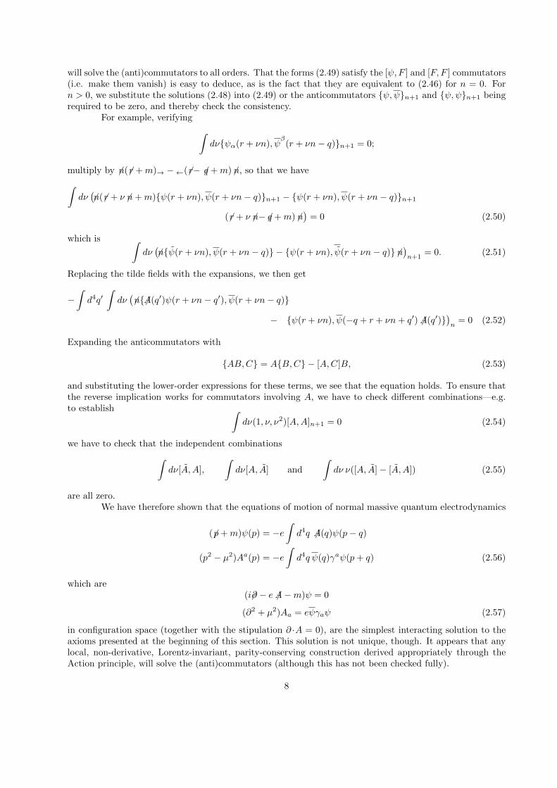
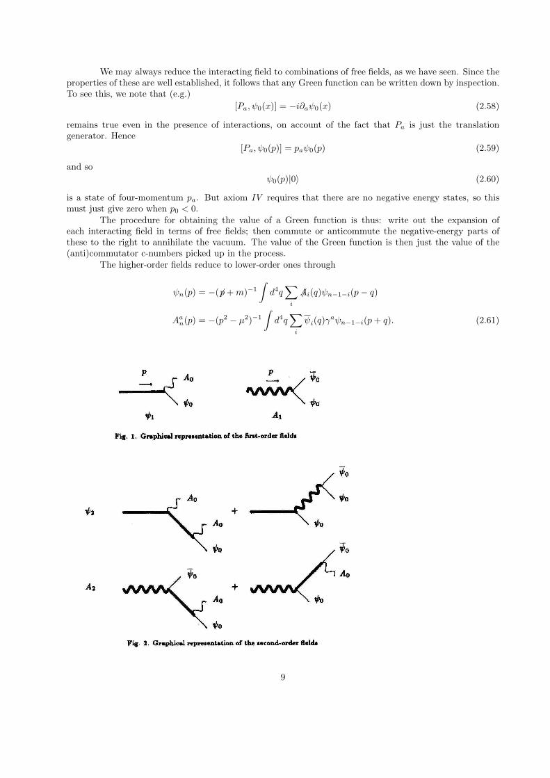
These can be viewed graphically as trees whose branches have free fields attached at the ends. Forexample, we can see ψ1 and A1 as the stems of fig. 1. We associate the factors −(6p+m)−1 and −(p2−µ2)−1

with the heavy lines, called “proliferators”. The second-order fields then have the representations shownin fig. 2, since we now attach one zeroth order and one first order field to the proliferator in each case.The higher order fields we obtain by continuing the process, i.e. adding further branches to the trees. Ina vacuum expectation value of a product of fields, the trees which represent each field link up through the(anti)commutation of the free fields to the right to annihilate the vacuum. This leads to the following set ofrules for obtaining the value of a Green function

2.3. THE GRAPH RULES

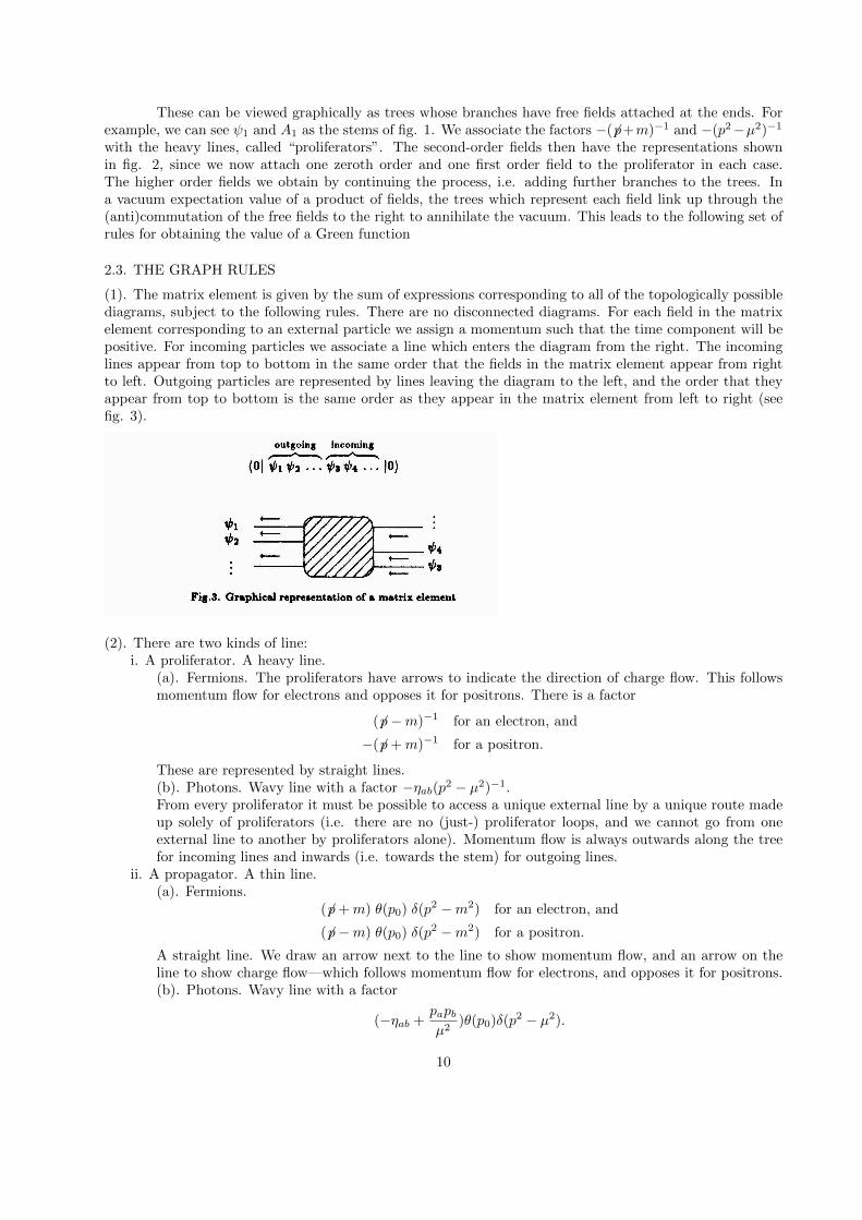
(1). The matrix element is given by the sum of expressions corresponding to all of the topologically possiblediagrams, subject to the following rules. There are no disconnected diagrams. For each field in the matrixelement corresponding to an external particle we assign a momentum such that the time component will bepositive. For incoming particles we associate a line which enters the diagram from the right. The incominglines appear from top to bottom in the same order that the fields in the matrix element appear from rightto left. Outgoing particles are represented by lines leaving the diagram to the left, and the order that theyappear from top to bottom is the same order as they appear in the matrix element from left to right (seefig. 3).

(2). There are two kinds of line:i. A proliferator. A heavy line.

(a). Fermions. The proliferators have arrows to indicate the direction of charge flow. This followsmomentum flow for electrons and opposes it for positrons. There is a factor

(6p−m)−1 for an electron, and

−(6p+m)−1 for a positron.

These are represented by straight lines.(b). Photons. Wavy line with a factor −ηab(p2 − µ2)−1.From every proliferator it must be possible to access a unique external line by a unique route madeup solely of proliferators (i.e. there are no (just-) proliferator loops, and we cannot go from oneexternal line to another by proliferators alone). Momentum flow is always outwards along the treefor incoming lines and inwards (i.e. towards the stem) for outgoing lines.

ii. A propagator. A thin line.(a). Fermions.

(6p+m) θ(p0) δ(p2 −m2) for an electron, and

(6p−m) θ(p0) δ(p2 −m2) for a positron.

A straight line. We draw an arrow next to the line to show momentum flow, and an arrow on theline to show charge flow—which follows momentum flow for electrons, and opposes it for positrons.(b). Photons. Wavy line with a factor

(−ηab +papbµ2

)θ(p0)δ(p2 − µ2).

10

We draw an arrow next to the line to show momentum flow.The direction of momentum flow in propagators is always from incoming to outgoing lines, or downwardsif between incoming proliferator trees, or upwards if between outgoing proliferator trees. Charge flow inthe proliferator trees is downwards in incoming trees. Propagators may attach at both ends to the sameproliferator tree. In this case we have to arrange that the momentum flow of the propagators is thendownwards. These directions become upwards for outgoing trees. Charge flow in loops is always clockwise.No line may cross a proliferator.

(3). The vertices are always the junctions of two fermion and one photon line. Four-momentum and chargeare conserved here, and a factor eγa is associated with it. There must be at least one proliferator joining thevertex.

(4). Spinor matrices are always contracted in the reverse order as they appear along a charge line. Thereis a factor (-1) for each crossing of fermion line by fermion line. For each graph, or connected subgraph,there is a momentum conservation factor δ(

∑pf −

∑pi). Undetermined momenta are integrated over (but

without an attached numerical factor).

2.4. THE INFINITIES AND THEIR REMOVAL

We obtain infinite answers for all physical quantities on account of higher order graphs. This meansthat the theory we have been developing cannot be the final answer. One hope is that these infinities area consequence of the expansion in the coupling constant, and if this could be avoided then they woulddisappear, but this is just speculation. For the time being we will “learn to live” with these since, if we do,we find that we reproduce Feynman graphs, at least, up to “tree” level, and these are known to give goodagreement with experiment.

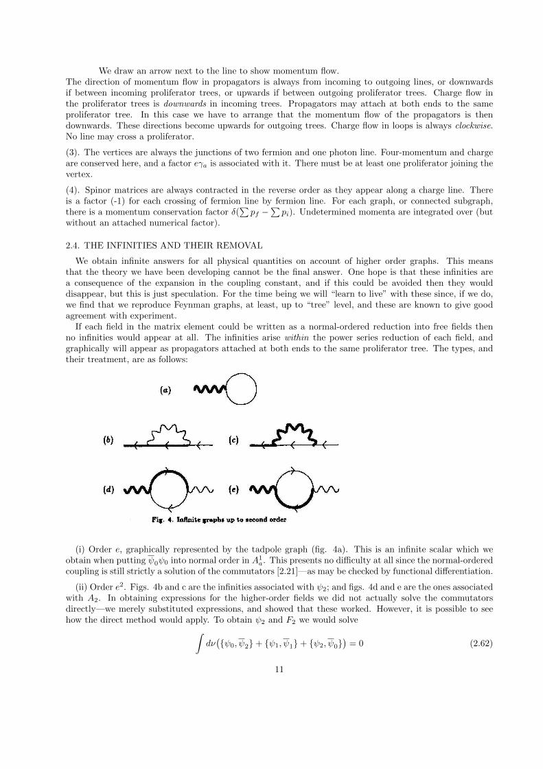
If each field in the matrix element could be written as a normal-ordered reduction into free fields thenno infinities would appear at all. The infinities arise within the power series reduction of each field, andgraphically will appear as propagators attached at both ends to the same proliferator tree. The types, andtheir treatment, are as follows:

(i) Order e, graphically represented by the tadpole graph (fig. 4a). This is an infinite scalar which weobtain when putting ψ0ψ0 into normal order in A1

a. This presents no difficulty at all since the normal-orderedcoupling is still strictly a solution of the commutators [2.21]—as may be checked by functional differentiation.

(ii) Order e2. Figs. 4b and c are the infinities associated with ψ2; and figs. 4d and e are the ones associatedwith A2. In obtaining expressions for the higher-order fields we did not actually solve the commutatorsdirectly—we merely substituted expressions, and showed that these worked. However, it is possible to seehow the direct method would apply. To obtain ψ2 and F2 we would solve∫

dν({ψ0, ψ2}+ {ψ1, ψ1}+ {ψ2, ψ0}

)= 0 (2.62)

11

together with {ψ,ψ}2, [ψ, F ]2 and [F, F ]2 being required to vanish. The middle term of (2.62) takes theform of a particular integral, and in analogy to the solution of the first-order case, we may derive

(6r∓ +m) 6n[

δ

δψ0(−s[±])

{ψ2(q − s[±]) +

∫d4q′

(6A(q′)ψ(q − s[±] − q′)

)1

}− δ

δψ0(r±)

{ψ2(r± − q) +

∫d4q′

(ψ(q′) 6A(q − r± + q′)

)1

}]6n(6s[∓] −m) = 0.

(2.63)

The second-order solution—as any higher order solution—is arbitrary to the extent of addition of a first-ordersolution. If we use the freedom available to include a first-order solution, then we are essentially modifyingthe equation of motion (such as (2.56)) to include local couplings of order e2 and higher. If we do not allowthis, then we are making each functional derivative in (2.63) separately zero, and may then integrate toobtain the expression for ψ2 that we had before [2.48]. However, these give the aforementioned infinities,which may only be avoided if we put the interactions ( 6Aψ)1 and (ψ 6A)1 in (2.63), in normal order. Wemust do this, so we have to subtract infinity times ψ0(q − s[±]) from the first interaction, and infinity times

ψ0(r± − q) in the other interaction. The tensors outside the main bracket have no effect, so what we arenow attempting to solve is thus

δ

δψ0(−s[±])

{ψ2(q − s[±]) +

∫d4q′ :

(6A(q′)ψ(q − s[±] − q′)

)1

:}

− δ

δψ0(r±)

{ψ2(r± − q) +

∫d4q′ :

(ψ(q′) 6A(q − r± + q′)

)1

:}

= indeterminate scalar (2.64)

since (∞)− (∞) is indeterminate.The LHS is of the form f(q, s[±]) − f(−q,−r±), so either the theory is inconsistent, or the scalar takes

the form s(q, s[±])− s∗(−q,−r±) and we are presented with the problem of solving

δ

δψ0(−s[±]){ψ2(q − s[±]) +

∫d4q′ :

(6A(q′)ψ(q − s[±] − q′)

)1

:}− s(q, s[±]) = C2(q).

(2.65)

We take C2(q) to be zero for reasons given earlier. The scalar must then be zero as will be seen when weput the resultant ψ2(p) on-shell and take vacuum expectation values. The same procedure may be appliedto the [F, F ]2 commutator to normal-order A2, and the commutators [ψ,ψ]2 and [ψ, F ]2 will still be zero.We may, therefore, ignore the divergent graphs.

(iii) Order e3 and higher. The foregoing may be extended to higher-order infinities, except that insteadof getting indeterminate scalars, we will normally get indeterminate operators, which, unlike the scalarsobtained before can in fact be legitimately integrated to make a contribution to the higher-order field.The indeterminacy means that this extra contribution is arbitrary except in the number and types of eachfield that it involves—so it may be a derivative or non-local construction, and as long as these appear innormal order, we cannot to exclude such contributions with complete rigour. We will exclude these terms onthe grounds that this is not the theory being considered: which is our argument for excluding higher thantrilinear couplings—which would be allowed from the solution of the commutators alone. Fundamentally, theproblem is that locality, as expressed by axiom VI is something that cannot unambiguously be demanded ofan interacting field theory. Our theory then represents what is apparently the simplest attempt at consistencywith (VI ) that is available in an interacting theory.

The consequence of all this, then, is that we delete all the infinite graphs which appear—which will alwaysbe ones where propagators are attached at both ends to the same proliferator tree (incidentally, finite graphs

12

of this kind must contain at least three photon proliferators in each loop, so they cannot appear until we aresolving for ψ6 or A7).

3. Scattering processes

We will consider the term “scattering” process to mean one where the particles involved behave as thoughfree for almost all of the time, interacting only briefly within some well-defined spatial region. In such asituation the amplitudes are well approximated by the lowest-order contributions to the matrix elements.We will consider the specific cases of e+e− elastic scattering and e+e− → γγγ, and then go on to the generalcase, showing that the lowest-order contributions to such processes are the same as those obtained from thetree-level Feynman graphs.

3.1. e+e− ELASTIC SCATTERING

The Green function we need is

〈0|ψα(t;−q1)ψβ(t;q2)ψγ(0;p2)ψ

δ(0;−p1)|0〉 =∫

dq01 dq02 dp

01 dp

02 e−i(q01+q

02)t 〈0|ψα(−q1)ψ

β(q2)ψγ(p2)ψ

δ(−p1)|0〉 (3.1)

The matrix element 〈0|ψα(−q1)ψβ(q2)ψγ(p2)ψ

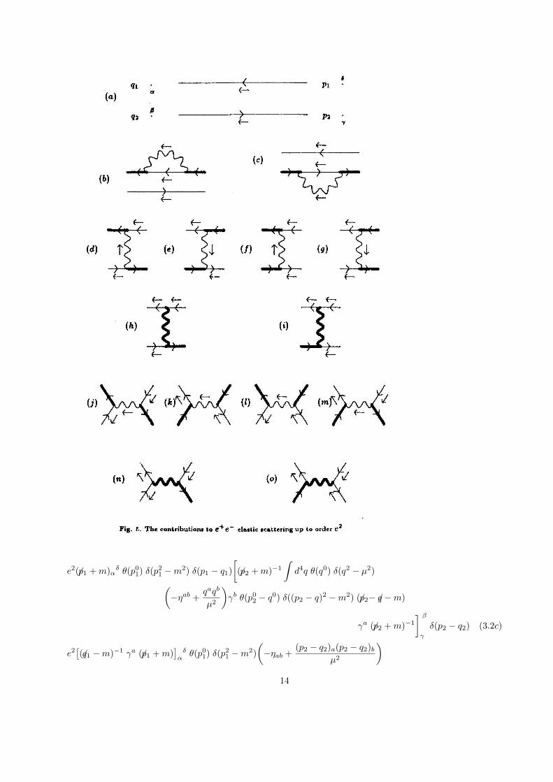
δ(−p1)|0〉 is, up to order e2, the sum of the following terms,

represented by the graphs of fig. 5:

(6p1 +m)αδ θ(p01)δ(p21 −m2) δ(p1 − q1) (6p2 −m)γ

β θ(p02)δ(p22 −m2) δ(p2 − q2) (3.2a)

e2[(6p1 −m)−1

∫d4q θ(q0)

(−ηab +

qaqb

µ2

)δ(q2 − µ2) γb θ(p01 − q0) δ((p1 − q)2 −m2)

(6p1−6q +m) γa (6p1 −m)−1] δα

δ(p1 − q1)

(6p2 −m)γβ θ(p02) δ(p22 −m2) δ(p2 − q2) (3.2b)

13

e2(6p1 +m)αδ θ(p01) δ(p21 −m2) δ(p1 − q1)

[(6p2 +m)−1

∫d4q θ(q0) δ(q2 − µ2)(

−ηab +qaqb

µ2

)γb θ(p02 − q0) δ((p2 − q)2 −m2) (6p2−6q −m)

γa (6p2 +m)−1] βγ

δ(p2 − q2) (3.2c)

e2[(6q1 −m)−1 γa (6p1 +m)

]αδ θ(p01) δ(p21 −m2)

(−ηab +

(p2 − q2)a(p2 − q2)bµ2

)14

θ(p02 − q02) δ((p2 − q2)2 − µ2)(−1)[(6p2 +m)−1 γb θ(q02) δ(q22 −m2) (6q2 −m)

]γβ

δ(q1 + q2 − p1 − p2) (3.2d)

plus corresponding expressions for the graphs e, f and g.

e2 θ(q01) δ(q21 −m2)[(6q1 +m) γa θ(p01) δ(p21 −m2) (6p1 +m)

]αδ −1

(p1 − q1)2 − µ2

(−1)[(6p2 +m)−1 γa θ(q

02) δ(q22 −m2) (6q2 −m)

]γβ δ(q1 + q2 − p1 − p2) (3.2h)

e2 θ(q01) δ(q21 −m2)[(6q1 +m) γa θ(p01) δ(p21 −m2) (6p1 +m)

]αδ −1

(p1 − q1)2 − µ2

θ(p02) δ(p22 −m2) (6p2 −m) γa (−1) (6q2 +m)−1]γβ δ(q1 + q2 − p1 − p2) (3.2i)

−e2[(6p2 +m)−1 γa θ(p

01) δ(p21 −m2) (6p1 +m)

]γδ

(−ηab +

(p1 + p2)a(p1 + p2)b

µ2

)θ(p01 + p02) δ((p1 + p2)2 − µ2)

[(6q1 −m)−1 γb (6q2 −m)

]αβ θ(q02) δ(q22 −m2)

δ(q1 + q2 − p1 − p2) (3.2j)

plus corresponding expressions for graphs k, l and m.

e2[(6q1 +m) θ(q01) δ(q21 −m2) γa (6q2 −m)

]αβ θ(q02) δ(q22 −m2)

−1

(p1 + p2)2 − µ2[−(6p2 +m)−1 γa θ(p01) δ(p21 −m2) (6p1 +m)

]γδ δ(q1 + q2 − p1 − p2) (3.2n)

e2[(6q1 +m) θ(q01) δ(q21 −m2) γa (−1) (6q2 +m)−1

]αβ −1

(p1 + p2)2 − µ2[(6p2 −m) θ(p02) δ(p22 −m2) γa θ(p01) δ(p21 −m2) (6p1 +m)

]γδ δ(q1 + q2 − p1 − p2) (3.2o)

The integrals in the self-energy graphs are just phase space integrals and so do not diverge. For example,graph (b) yields

πe2

2p21θ(p01 −

√p21 + (m+ µ)2

) √(p21 − (µ+m)2)(p21 − (µ−m)2)[(

−6p1 + 3m− (p21 −m2 − 2µ2)(p21 + µ2 −m2)

2µ2p216p1)

(6p1 −m)−1] δα

δ(p1 − q1) (6p2 −m)γβ θ(p02) δ(p22 −m2) δ(p2 − q2) (3.3)

The contribution that this gives to the matrix element (3.1) is then

δ(p2 − q2) (6p2 −m)γβ 1

2p02eip

02t

∣∣∣∣p02=√

p22+m

2

δ(p1 − q1)∫ ∞√

p21+(m+µ)2

dp01 eip01t

πe2

2p21(−6p1 +m)

√p21 − (µ+m)2

√p21 − (µ−m)2

[(−6p1 + 3m− (p21 −m2 − 2µ2)(p21 + µ2 −m2)

2µ2p216p1)

(6p1 −m)−1] δα

(3.4)

Over the range considered, i.e.√p21 + (m+ µ)2 to infinity, the integrand is a continuous, smooth function,

vanishing at the limits. Hence the Fourier transform is a function which vanishes at the limits. The way tosee this is that the Fourier transform is a reduction of a function into harmonic waves, and so if the functionis smooth, then there will be a limit to the frequency of the waves used in its composition. Thus the F.T.vanishes as t→∞. If the F.T. is not to vanish then there must be infinite frequency parts, i.e. singularities.Therefore the graph just gives a “transient”—a contribution which disappears as t becomes large. This willhave no effect on the calculation of scattering amplitudes.

If we imagine that the matrix elements are integrated with suitably smooth wave functions in both theinitial and final states, then we find that all of the associated graphs lead to transients, except for the ones

15

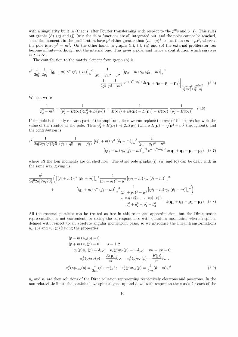
with a singularity built in (that is, after Fourier transforming with respect to the p0’s and q0’s). This rulesout graphs (d)–(g) and (j)–(m): the delta functions are all integrated out, and the poles cannot be reached,since the momenta in the proliferators have p2 either greater than (m+ µ)2 or less than (m− µ)2, whereasthe pole is at p2 = m2. On the other hand, in graphs (h), (i), (n) and (o) the external proliferator canbecome infinite—although not the internal one. This gives a pole, and hence a contribution which survivesas t→∞.

The contribution to the matrix element from graph (h) is

e21

2q01

1

2p01

[(6q1 +m) γa (6p1 +m)

]αδ 1

(p1 − q1)2 − µ2

[(6p2 −m) γa (6q2 −m)

]γβ

1

2q02

1

p22 −m2e−i(q

01+q

02)t δ(q1 + q2 − p1 − p2)

∣∣∣∣p1,q1,q2 onshell

p02=q01+q

02−p

01

(3.5)

We can write

1

p22 −m2=

1

(p02 − E(p2))(p02 + E(p2))=

1

E(q1) + E(q2)− E(p1)− E(p2)

1

(p02 + E(p2))(3.6)

If the pole is the only relevant part of the amplitude, then we can replace the rest of the expression with thevalue of the residue at the pole. Thus p02 + E(p2) → 2E(p2) (where E(p) =

√p2 +m2 throughout), and

the contribution is

e21

2q012q022p012p02

1

(q01 + q02 − p01 − p02)

[(6q1 +m) γa (6p1 +m)

]αδ 1

(p1 − q1)2 − µ2[(6p2 −m) γa (6q2 −m)

]γβ e−i(q

01+q

02)t δ(q1 + q2 − p1 − p2) (3.7)

where all the four momenta are on shell now. The other pole graphs (i), (n) and (o) can be dealt with inthe same way, giving us

e2

2q012q022p012p02

([(6q1 +m) γa (6p1 +m)

]αδ 1

(p1 − q1)2 − µ2

[(6p2 −m) γa (6q2 −m)

]γβ

+[(6q1 +m) γa (6q2 −m)

]αβ 1

(p1 + p2)2 − µ2

[(6p2 −m) γa (6p1 +m)

]γδ

)e−i(q

01+q

02)t − e−i(p01+p02)t

q01 + q02 − p01 − p02δ(q1 + q2 − p1 − p2) (3.8)

All the external particles can be treated as free in this resonance approximation, but the Dirac tensorrepresentation is not convenient for seeing the correspondence with quantum mechanics, wherein spin isdefined with respect to an absolute angular momentum basis, so we introduce the linear transformationsusα(p) and vsα(p) having the properties

(6p−m) us(p) = 0

(6p+m) vs(p) = 0 s = 1, 2

us(p)us′(p) = δss′ ; vs(p)vs′(p) = −δss′ ; vu = uv = 0;

u+s (p)us′(p) =E(p)

mδss′ ; v+s (p)vs′(p) =

E(p)

mδss′ ;

uβs (p)usα(p) =1

2m(6p+m)α

β ; vβs (p)vsα(p) =1

2m(6p−m)α

β (3.9)

us and vs are then solutions of the Dirac equation representing respectively electrons and positrons. In thenon-relativistic limit, the particles have spins aligned up and down with respect to the z-axis for each of the

16

values of s. Contracting these spinors appropriately with (3.8), and adding the zeroth-order contribution,we get

m2

p01p02

δr1s1 δ(p1 − q1) δr2s2 δ(p2 − q2) e−i(p01+p

02)t

+e2m4

q01q02p

01p

02

(us1(q1) γa ur1(p1)

1

(p1 − q1)2 − µ2vr2(p2) γa vs2(q2)

+ us1(q1) γa vs2(q2)1

(p1 + p2)2 − µ2vr2(p2) γa ur1(p1)

)δ(q1 + q2 − p1 − p2)

e−i(q01+q

02)t − e−i(p01+p02)t

q01 + q02 − p01 − p02(3.10)

This is to be compared with

〈q1, s1;q2, s2|eiHt|p2, r2;p1, r1〉 = ei(p01+p

02)t δr1s1 δ(q1 − p1) δr2s2 δ(q2 − p2)

+ 〈q1, s1;q2, s2|V |p2, r2;p1, r1〉ei(q

01+q

02)t − ei(p01+p02)t

q01 + q02 − p01 − p02+O(V 2) (3.11)

Which we have in the purely quantum mechanical interpretation of the same system. Evidently, within theresonance approximation, up to this order, the interaction picture does exist, since a direct comparison showsthat the expressions are the same (apart from a differing sign of t, which is irrelevant). If we define

|p2, r2;p1, r1〉 =

√p01p

02

m2vr2(p2)ψ(0;p2) ψ(0;p1)ur1(p1)|0〉 (3.12)

then (3.10) takes the same form as (3.11), with

〈q1, s1;q2, s2|V |p2, r2;p1, r1〉 =e2m2√q01q

02p

01p

02

(us1(q1) γa ur1(p1)

1

(p1 − q1)2 − µ2

vr2(p2) γa vs2(q2) + us1(q1) γa vs2(q2)1

(p1 + p2)2 − µ2vr2(p2) γa ur1(p1)

)δ(q1 + q2 − p1 − p2) (3.13)

The differential cross section for scattering of beams of different particles of momenta p1 and p2 and spinpolarisations r1 and r2, into momentum space regions d3q1 and d3q2, with spin polarisations s1 and s2 isgiven by ordinary quantum mechanicsas

dσ =1

vd3q1d

3q2|〈q1, s1;q2, s2‖V ‖p2, r2;p1, r1〉|2 (2π)4 δ(q1 + q2 − p1 − p2) (3.14)

where v is the velocity of one particle beam in a frame where the other is stationary, and the “double bar”matrix element is one where the three momentum conservation delta function has been extracted.

Hence

dσ =1

v

m

q01d3q1

m

q02d3q2

m

p01

m

p02

e4∣∣∣∣us1(q1) γa ur1(p1)

1

(p1 − q1)2 − µ2vr2(p2) γa vs2(q2) +

us1(q1) γa vs2(q2)1

(p1 + p2)2 − µ2vr2(p2) γa ur1(p1)

∣∣∣∣2(2π)4 δ(q1 + q2 − p1 − p2) (3.16)

17

The normalisations have been chosen so as to avoid factors of (2π)3 appearing whenever possible; this meansthat we need to replace

ψ → (2π)32ψ; A→ (2π)

32A; e→ (2π)−

32 e (3.17)

to compare with the usual formulation. This gives

dσ =1

v

m

p01

m

p02

d3q1

(2π)3m

q01

d3q2

(2π)3m

q02

e4∣∣∣∣us1(q1) γa ur1(p1)

1

(p1 − q1)2 − µ2vr2(p2) γa vs2(q2) +

us1(q1) γa vs2(q2)1

(p1 + p2)2 − µ2vr2(p2) γa ur1(p1)

∣∣∣∣2(2π)4 δ(q1 + q2 − p1 − p2) (3.18)

which is exactly what we obtain from the consideration of the Feynman graphs of fig. 6.

3.2. e+e− → γγγ

18

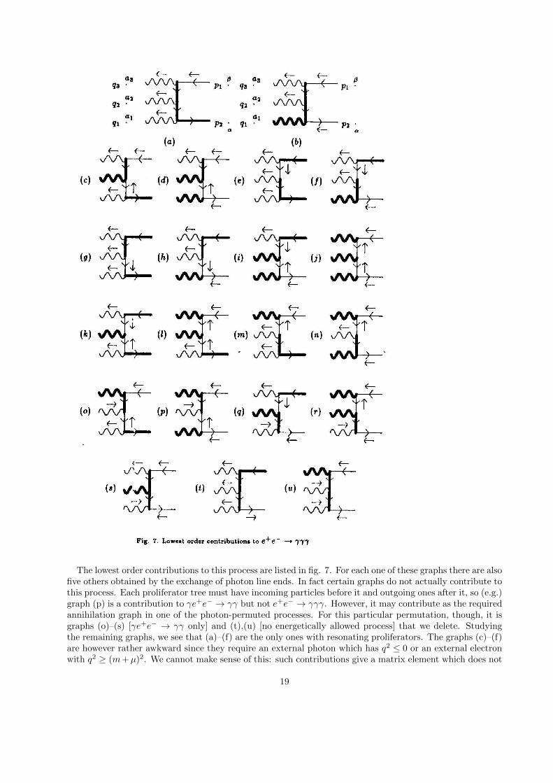
The lowest order contributions to this process are listed in fig. 7. For each one of these graphs there are alsofive others obtained by the exchange of photon line ends. In fact certain graphs do not actually contribute tothis process. Each proliferator tree must have incoming particles before it and outgoing ones after it, so (e.g.)graph (p) is a contribution to γe+e− → γγ but not e+e− → γγγ. However, it may contribute as the requiredannihilation graph in one of the photon-permuted processes. For this particular permutation, though, it isgraphs (o)–(s) [γe+e− → γγ only] and (t),(u) [no energetically allowed process] that we delete. Studyingthe remaining graphs, we see that (a)–(f) are the only ones with resonating proliferators. The graphs (c)–(f)are however rather awkward since they require an external photon which has q2 ≤ 0 or an external electronwith q2 ≥ (m+µ)2. We cannot make sense of this: such contributions give a matrix element which does not

19

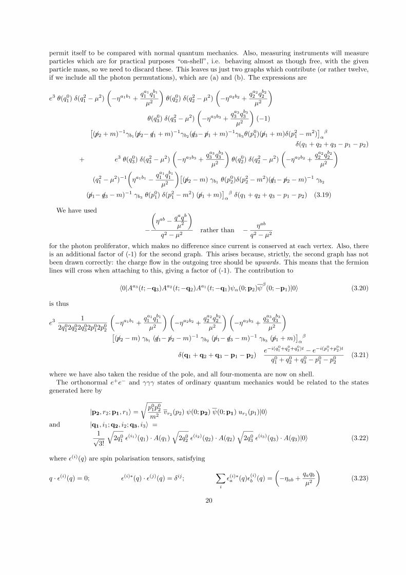
permit itself to be compared with normal quantum mechanics. Also, measuring instruments will measureparticles which are for practical purposes “on-shell”, i.e. behaving almost as though free, with the givenparticle mass, so we need to discard these. This leaves us just two graphs which contribute (or rather twelve,if we include all the photon permutations), which are (a) and (b). The expressions are

e3 θ(q01) δ(q21 − µ2)

(−ηa1b1 +

qa11 qb11µ2

)θ(q02) δ(q22 − µ2)

(−ηa2b2 +

qa22 qb22µ2

)θ(q03) δ(q23 − µ2)

(−ηa3b3 +

qa33 qb33µ2

)(−1)[

(6p2 +m)−1γb1(6p2−6q1 +m)−1γb2(6q3−6p1 +m)−1γb3θ(p01)(6p1 +m)δ(p21 −m2)

]αβ

δ(q1 + q2 + q3 − p1 − p2)

+ e3 θ(q03) δ(q23 − µ2)

(−ηa3b3 +

qa33 qb33µ2

)θ(q02) δ(q22 − µ2)

(−ηa2b2 +

qa22 qb22µ2

)(q21 − µ2)−1

(ηa1b1 − qa11 qb11

µ2

)[(6p2 −m) γb1 θ(p

02)δ(p22 −m2)(6q1−6p2 −m)−1 γb2

(6p1−6q3 −m)−1 γb3 θ(p01) δ(p21 −m2) (6p1 +m)

]αβ δ(q1 + q2 + q3 − p1 − p2) (3.19)

We have used

−

(ηab − qaqb

µ2

)q2 − µ2

rather than − ηab

q2 − µ2

for the photon proliferator, which makes no difference since current is conserved at each vertex. Also, thereis an additional factor of (-1) for the second graph. This arises because, strictly, the second graph has notbeen drawn correctly: the charge flow in the outgoing tree should be upwards. This means that the fermionlines will cross when attaching to this, giving a factor of (-1). The contribution to

〈0|Aa3(t;−q3)Aa2(t;−q2)Aa1(t;−q1)ψα(0;p2)ψβ(0;−p1)|0〉 (3.20)

is thus

e31

2q012q022q032p012p02

(−ηa1b1 +

qa11 qb11µ2

) (−ηa2b2 +

qa22 qb22µ2

) (−ηa3b3 +

qa33 qb33µ2

)[(6p2 −m) γb1 (6q1−6p2 −m)−1 γb2 (6p1−6q3 −m)−1 γb3 (6p1 +m)

]αβ

δ(q1 + q2 + q3 − p1 − p2)e−i(q

01+q

02+q

03)t − e−i(p01+p02)t

q01 + q02 + q03 − p01 − p02(3.21)

where we have also taken the residue of the pole, and all four-momenta are now on shell.The orthonormal e+e− and γγγ states of ordinary quantum mechanics would be related to the states

generated here by

|p2, r2;p1, r1〉 =

√p01p

02

m2vr2(p2) ψ(0;p2) ψ(0;p1) ur1(p1)|0〉

and |q1, i1;q2, i2;q3, i3〉 =

1√3!

√2q01 ε

(i1)(q1) ·A(q1)√

2q02 ε(i2)(q2) ·A(q2)

√2q03 ε

(i3)(q3) ·A(q3)|0〉 (3.22)

where ε(i)(q) are spin polarisation tensors, satisfying

q · ε(i)(q) = 0; ε(i)∗(q) · ε(j)(q) = δij ;∑i

ε(i)∗a (q)ε(i)b (q) =

(−ηab +

qaqbµ2

)(3.23)

20

This gives us a quantum-mechanics-style reduced matrix element for the process thus:

〈q1, i1;q2, i2;q3, i3‖V ‖p2, r2;p1, r1〉 =e3√

2q012q022q03

√m2

p01p02

1√3!

(ε(i1)∗b1(q1) ε(i2)∗b2(q2) ε(i3)∗b3(q3) + 5 exchanges

)vr2(p2) γb1 (6q1−6p2 −m)−1 γb2 (6p1−6q3 −m)−1 γb3 ur1(p1) (3.24)

and hence a differential cross-section of

dσ =1

v

d3q1

2q01

d3q2

2q02

d3q3

2q03

m

p01

m

p02

1

3!∣∣∣∣e3 (ε(i1)∗b1(q1) ε(i2)∗b2(q2) ε(i3)∗b3(q3) + 5 exchanges)

vr2(p2) γb1 (6q1−6p2 −m)−1 γb2 (6p1−6q3 −m)−1 γb3 ur1(p1)

∣∣∣∣2(2π)4 δ(q1 + q2 + q3 − p1 − p2) (3.25)

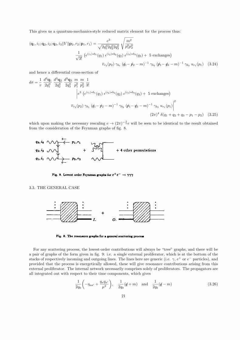
which upon making the necessary rescaling e → (2π)−32 e will be seen to be identical to the result obtained

from the consideration of the Feynman graphs of fig. 8.

3.3. THE GENERAL CASE

For any scattering process, the lowest-order contributions will always be “tree” graphs, and there will bea pair of graphs of the form given in fig. 9: i.e. a single external proliferator, which is at the bottom of thestacks of respectively incoming and outgoing lines. The lines here are generic (i.e. γ, e+ or e− particles), andprovided that the process is energetically allowed, these will give resonance contributions arising from thisexternal proliferator. The internal network necessarily comprises solely of proliferators. The propagators areall integrated out with respect to their time components, which gives

1

2q0

(−ηaa′ +

qaqa′

µ2

),

1

2q0(6q +m) and

1

2q0(6q −m) (3.26)

21

for the cases of photons, electrons and positrons respectively (where all momenta are on shell). The inte-gration of the time component of the proliferator momentum is done by the time-component part of thefour-momentum delta function. This gives an energy conservation resonance pole. Taking the residue of thisin the rest of the expression, we have

(∓)1

2q0

(−ηaa′ +

qaqa′

µ2

)1

Ef − Ei, (∓)

1

2q0(6q +m)

1

Ef − Ei

and (±)1

2q0(6q −m)

1

Ef − Ei(3.27)

for photons, electrons and positrons. The top sign is for appearance in the final state, the bottom forappearance in the initial state. In the resonance approximation, the value of the internal expression is thesame for each graph, apart from a possible sign. This arises because charge in a proliferator tree attachedto an incoming line flows downwards, whereas in an outgoing tree it flows upwards, and in going from oneto the other we may cause fermion lines to cross of uncross, each one generating a factor of (-1). A rather

involved argument shows us that the difference between the two internal expressions is (−1)e+I+e+

O , where e+Iis unity if the proliferator I is a positron and zero otherwise. Similarly for e+O. This is because of fermionline crossings. Hence the value of the resonance parts of the two graphs is

(−)e+Ie−iEf t − e−iEit

Ef − Ei(outgoing factors) (internal expression) (incoming factors) (3.28)

(the “internal expression” applying to the graph with the incoming proliferator). The factors applied to theinternal expression are of the form of propagators, i.e. those of (3.26) which includes the place where theproliferator was before.

To relate this matrix element to one of ordinary quantum mechanics, we need to multiply incoming linesby √

2q0 ε(i)a (q),

√q0mur(q) and

√q0mvr(q) (3.29)

for respectively photons, electrons and positrons. The Pauli adjoints of these are applied to outgoing lines.Contracting these with the factors obtained before, we then have

− 1√2q0

ε(i)a (q),

√m

q0ur(q) and −

√m

q0vr(q) (3.30)

as the factors to be applied to the internal expression, the adjoints being used for outgoing lines. There isalso a factor of 1/

√m! for each m-repeated incoming or outgoing particle.

If we include the external proliferator, then we can imagine the graph as built up with the rules

i6q −m for internal fermion lines, where q is the

momentum flowing parallel to the charge line

−iηabq2 − µ2 for internal photon lines

−ieγa for each vertex

which are those of ordinary Feynman graph analysis. This follows because the number or vertices is thesame as the number of proliferators, so the i discrepancy in the lines multiplies the −i discrepancy in thevertices to give no overall change. However the external proliferator is put on shell so an extra factor of i isspare. The matrix element is thus

e−iEf t − e−iEit

Ef − Eii(−)nγ+ne+

√S

(m

q0

)(ne++ne− )/2 (1

2q0

)nγ/2[Feynman graph amplitude] (3.31)

22

where ne± are the total number of external e± lines and nγ is the total number of external photon lines.

S =∏i

1

mi!

is the factor for repeated particles of the same type. The (−)e+I belongs to the Feynman amplitude: if we

look closely at the S-matrix reduction, we see that the signs from fermion crossings are the same exceptthat the incoming proliferator is not treated any differently to the other lines and so the charge line which isgenerated will have a loop in it if it is a positron (to make it flow the right way into the vertex), and hencea sign.

We may now sum all of the amplitudes if more than one graph contributes to the process. We may alsomake the rescaling e → (2π)−

32 e. The number of vertices is two greater than the number of external lines

(since it is built of ‘tree’ diagrams). Also, there are two incoming lines, so the effect of the rescaling is toput factors of (2π)−3 on each outgoing line. Thus the cross-section for the process is given by

dσ =1

v(incoming factors) |M|2 (outgoing factors)(2π)4 δ(p1 + p2 −

n∑i=1

qi) S (3.32)

where the incoming factors are 1/2p0 for a photon and m/p0 for a fermion. The outgoing factors ared3q/((2π)32q0) for photons and d3q/(2π)3(m/q0) for fermions. M is the sum of Feynman graphs and S isthe statistical factor

S =∏i

1

mi!

for each mi-repeated particle type, but this time only over the final state particles. The factor 12 from

possible identical particles in the initial state is cancelled by a factor of two which appears in the quantummechanical cross-section formula for this case.

What we have written down, of course, is none other than the cross-section arising from the tree Feynmangraphs for the process in question.

4. Conclusion and outlook

In formulating any physical theory it is necessary to start by eliminating that which is definitely wrong,and then to find what could be right from whatever is left. This process is painful in the case of relativisticquantum field theory as, at present, nothing is left. A theory which is plagued with infinities is definitelywrong, as is a theory which violates Haag’s theorem. The author nurtured the hope, at least initially, thatcuring one would also cure the other, but this was clearly misguided. This is necessarily so, as we are simplynot allowed to expand in the coupling constant. To see this, try expanding a wave function of the Hydrogenatom out in powers of e and see how much sense that makes.

So, to conclude, we have a technique which at best solves some important problems of quantum fieldtheory, and provides a pointer to a possible future theory which is completely free from infinities. At worst itsimply reminds us that, over sixty years after it was first thought of, we still have no interacting relativisticquantum field theory.

References

[1] Hall, D. and Wightman, A., Mat. Fys. Medd. Dansk. Vid. Selskapet 31 5 (1957)See also Streater, R. and Wightman, A., PCT, spin, statistics and all that.p. 165. Benjamin-Cummings, N.Y., 1979

[2] Oakley, C., ‘Does the interaction picture exist?’ Hatfield Polytechnic preprint, 1986

The ‘usual formulation of Q.E.D.’ means that presented inBjorken, J. and Drell, S., Relativistic quantum fields, McGraw-Hill, 1965 orItzykson, C., and Zuber, J.-B., Quantum field theory, McGraw-Hill, 1980

23