quantum corrections to gravity and implications for...
TRANSCRIPT
Quantum corrections to gravity and implicationsfor cosmology and astrophysics
Ilya L. Shapiro
Departamento de Física, Universidade Federal de Juiz de Fora, MG, Brazil
Based on collaborations with
|P. Letelier| (UNICAMP), D. Rodrigues (UFES), J. Solà (UB)J. Fabris (UFES), A. Toribio (UFES).
QFEXT-2011 – Benasque – September, 2011
Ilya Shapiro, Quantum corrections and implications for cosmology and astrophysics

Contents:
• Effective Action of vacuum for QFEXT / gravity.
• Quantum corrections to vacuum action for massless fields.
• Quantum corrections to vacuum action for massive fields.
• Renormalization Group for ρΛ and G.
• Interpretation of µ in case of galaxies.
• Do we have a chance for an alternative concordance model?.
Ilya Shapiro, Quantum corrections and implications for cosmology and astrophysics
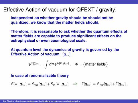
Effective Action of vacuum for QFEXT / gravity.Independent on whether gravity should be should not bequantized, we know that the matter fields should.
Therefore, it is reasonable to ask whether the quantum effects ofmatter fields are capable to produce significant effects on theastrophysical or even cosmological scale.
At quantum level the dynamics of gravity is governed by theEffective Action of vacuum Γ[gµν ].
eiΓ[gµν ] =
∫dΦeiS[Φ, gµν ] , Φ =
matter fields
.
In case of renormalizable theory
S[Φ, gµν ] = Svac[gµν ]+Sm[Φ, gµν ] ⇒ Γ[gµν ] = Svac[gµν ]+ Γ[gµν ] .
Ilya Shapiro, Quantum corrections and implications for cosmology and astrophysics
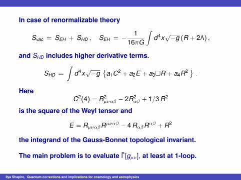
In case of renormalizable theory
Svac = SEH + SHD , SEH = − 116πG
∫d4x
√−g (R + 2Λ) ,
and SHD includes higher derivative terms.
SHD =
∫d4x
√−g
a1C2 + a2E + a3R + a4R2 .
HereC2(4) = R2
µναβ − 2R2αβ + 1/3 R2
is the square of the Weyl tensor and
E = RµναβRµναβ − 4 RαβRαβ + R2
the integrand of the Gauss-Bonnet topological invariant.
The main problem is to evaluate Γ[gµν ], at least at 1-loop.
Ilya Shapiro, Quantum corrections and implications for cosmology and astrophysics
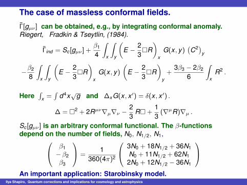
The case of massless conformal fields.
Γ[gµν ] can be obtained, e.g., by integrating conformal anomaly.Riegert, Fradkin & Tseytlin, (1984).
Γind = Sc[gµν ] +β1
4
∫x
∫y
(E − 2
3R)
xG(x , y)
(C2)
y
−β2
8
∫x
∫y
(E − 2
3R)
xG(x , y)
(E − 2
3R)
y+
3β3 − 2β2
6
∫x
R2 .
Here∫
x =∫
d4x√
g and ∆xG(x , x ′) = δ(x , x ′) .
∆ = 2 + 2Rµν∇µ∇ν − 23
R+13(∇µR)∇µ .
Sc[gµν ] is an arbitrary conformal functional. The β-functionsdepend on the number of fields, N0, N1/2, N1, β1
−β2β3
=1
360(4π)2
3N0 + 18N1/2 + 36N1N0 + 11N1/2 + 62N12N0 + 12N1/2 − 36N1
An important application: Starobinsky model.
Ilya Shapiro, Quantum corrections and implications for cosmology and astrophysics
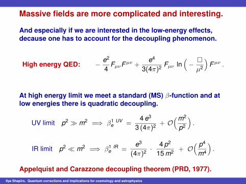
Massive fields are more complicated and interesting.
And especially if we are interested in the low-energy effects,decause one has to account for the decoupling phenomenon.
High energy QED: − e2
4FµνFµν +
e4
3(4π)2 Fµν ln(−
µ2
)Fµν .
At high energy limit we meet a standard (MS) β-function and atlow energies there is quadratic decoupling.
UV limit p2 ≫ m2 =⇒ β1 UVe =
4 e3
3 (4π)2 + O(m2
p2
).
IR limit p2 ≪ m2 =⇒ β1 IRe =
e3
(4π)2 · 4 p2
15 m2 + O( p4
m4
).
Appelquist and Carazzone decoupling theorem (PRD, 1977).
Ilya Shapiro, Quantum corrections and implications for cosmology and astrophysics
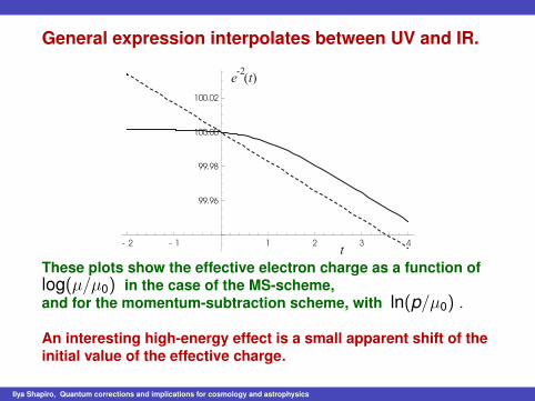
General expression interpolates between UV and IR.
e t( )-2
t
These plots show the effective electron charge as a function oflog(µ/µ0) in the case of the MS-scheme,and for the momentum-subtraction scheme, with ln(p/µ0) .
An interesting high-energy effect is a small apparent shift of theinitial value of the effective charge.
Ilya Shapiro, Quantum corrections and implications for cosmology and astrophysics
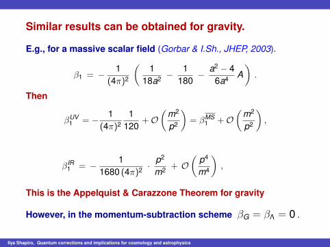
Similar results can be obtained for gravity.
E.g., for a massive scalar field (Gorbar & I.Sh., JHEP, 2003).
β1 = − 1(4π)2
(1
18a2 − 1180
− a2 − 46a4 A
).
Then
βUV1 = − 1
(4π)21
120+O
(m2
p2
)= βMS
1 +O(
m2
p2
),
βIR1 = − 1
1680 (4π)2 · p2
m2 + O(
p4
m4
),
This is the Appelquist & Carazzone Theorem for gravity
However, in the momentum-subtraction scheme βG = βΛ = 0 .
Ilya Shapiro, Quantum corrections and implications for cosmology and astrophysics
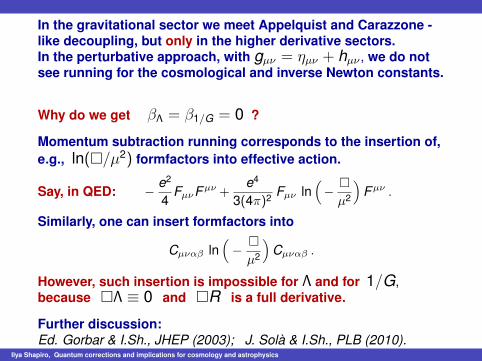
In the gravitational sector we meet Appelquist and Carazzone -like decoupling, but only in the higher derivative sectors.In the perturbative approach, with gµν = ηµν + hµν , we do notsee running for the cosmological and inverse Newton constants.
Why do we get βΛ = β1/G = 0 ?
Momentum subtraction running corresponds to the insertion of,e.g., ln(/µ2) formfactors into effective action.
Say, in QED: − e2
4FµνFµν +
e4
3(4π)2 Fµν ln(−
µ2
)Fµν .
Similarly, one can insert formfactors into
Cµναβ ln(−
µ2
)Cµναβ .
However, such insertion is impossible for Λ and for 1/G,because Λ ≡ 0 and R is a full derivative.
Further discussion:Ed. Gorbar & I.Sh., JHEP (2003); J. Solà & I.Sh., PLB (2010).
Ilya Shapiro, Quantum corrections and implications for cosmology and astrophysics
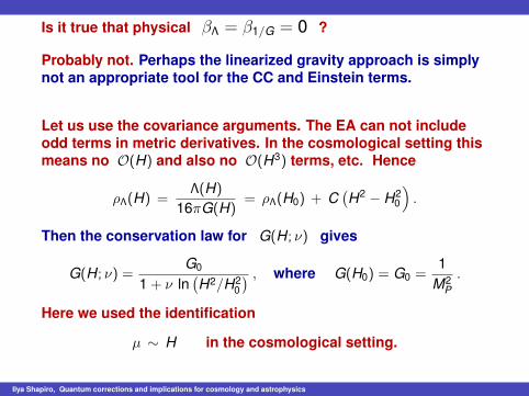
Is it true that physical βΛ = β1/G = 0 ?
Probably not. Perhaps the linearized gravity approach is simplynot an appropriate tool for the CC and Einstein terms.
Let us use the covariance arguments. The EA can not includeodd terms in metric derivatives. In the cosmological setting thismeans no O(H) and also no O(H3) terms, etc. Hence
ρΛ(H) =Λ(H)
16πG(H)= ρΛ(H0) + C
(H2 − H2
0
).
Then the conservation law for G(H; ν) gives
G(H; ν) =G0
1 + ν ln(H2/H2
0
) , where G(H0) = G0 =1
M2P.
Here we used the identification
µ ∼ H in the cosmological setting.
Ilya Shapiro, Quantum corrections and implications for cosmology and astrophysics
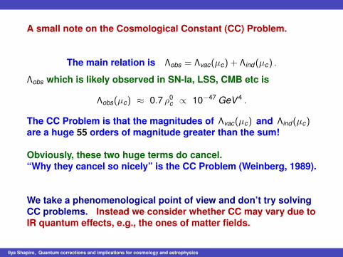
A small note on the Cosmological Constant (CC) Problem.
The main relation is Λobs = Λvac(µc) + Λind (µc) .
Λobs which is likely observed in SN-Ia, LSS, CMB etc is
Λobs(µc) ≈ 0.7 ρ0c ∝ 10−47 GeV 4 .
The CC Problem is that the magnitudes of Λvac(µc) and Λind (µc)are a huge 55 orders of magnitude greater than the sum!
Obviously, these two huge terms do cancel.“Why they cancel so nicely” is the CC Problem (Weinberg, 1989).
We take a phenomenological point of view and don’t try solvingCC problems. Instead we consider whether CC may vary due toIR quantum effects, e.g., the ones of matter fields.
Ilya Shapiro, Quantum corrections and implications for cosmology and astrophysics
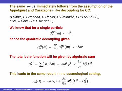
The same ρΛ(µ) immediately follows from the assumption of theAppelquist and Carazzone - like decoupling for CC.
A.Babic, B.Guberina, R.Horvat, H.Štefancic, PRD 65 (2002);I.Sh., J.Solà, JHEP 02 (2002).
We know that for a single particle
βMSΛ (m) ∼ m4 ,
hence the quadratic decoupling gives
βIRΛ (m) =
µ2
m2 βMSΛ (m) ∼ µ2m2 .
The total beta-function will be given by algebraic sum
βIRΛ =
∑kiµ
2m2i = σM2 µ2 ∝ 3ν
8πM2
P H2 .
This leads to the same result in the cosmological setting,
ρΛ(H) = ρΛ(H0) +3ν8π
M2p(H2 − H2
0
).
Ilya Shapiro, Quantum corrections and implications for cosmology and astrophysics

One can also obtain the same G(µ) in a different way.
I.Sh., J. Solà, JHEP (2002); C. Farina, I.Sh. et al, PRD (2011).
Consider MS-based renormalization group equation for G(µ):
µdG−1
dµ=
∑particles
Aij mi mj = 2ν M2P , G−1(µ0) = G−1
0 = M2P .
Here the coefficients Aij depend on the coupling constants,mi are masses of all particles. In particular, at one loop,∑
particles
Aij mi mj =∑
fermions
m2f
3(4π)2 −∑
scalars
m2s
(4π)2
(ξs −
16
).
One can rewrite it as
µd(G/G0)
dµ= −2ν (G/G0)
2 , =⇒ G(µ) =G0
1 + ν ln(µ2/µ2
0
) . (∗)
It is the same formula which results from covariance and/or fromAC-like quadratic decoupling for the CC plus conservation law.All in all, (*) seems to a unique possible form of a relevant G(µ).
Ilya Shapiro, Quantum corrections and implications for cosmology and astrophysics
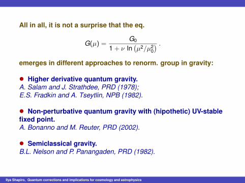
All in all, it is not a surprise that the eq.
G(µ) =G0
1 + ν ln(µ2/µ2
0
) .emerges in different approaches to renorm. group in gravity:
• Higher derivative quantum gravity.A. Salam and J. Strathdee, PRD (1978);E.S. Fradkin and A. Tseytlin, NPB (1982).
• Non-perturbative quantum gravity with (hipothetic) UV-stablefixed point.A. Bonanno and M. Reuter, PRD (2002).
• Semiclassical gravity.B.L. Nelson and P. Panangaden, PRD (1982).
Ilya Shapiro, Quantum corrections and implications for cosmology and astrophysics
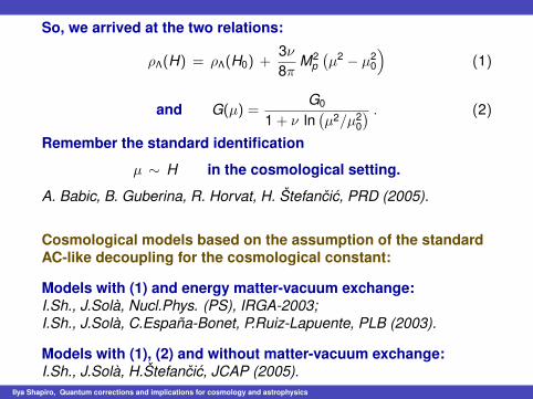
So, we arrived at the two relations:
ρΛ(H) = ρΛ(H0) +3ν8π
M2p(µ2 − µ2
0
)(1)
and G(µ) =G0
1 + ν ln(µ2/µ2
0
) . (2)
Remember the standard identification
µ ∼ H in the cosmological setting.
A. Babic, B. Guberina, R. Horvat, H. Štefancic, PRD (2005).
Cosmological models based on the assumption of the standardAC-like decoupling for the cosmological constant:
Models with (1) and energy matter-vacuum exchange:I.Sh., J.Solà, Nucl.Phys. (PS), IRGA-2003;I.Sh., J.Solà, C.España-Bonet, P.Ruiz-Lapuente, PLB (2003).
Models with (1), (2) and without matter-vacuum exchange:I.Sh., J.Solà, H.Štefancic, JCAP (2005).
Ilya Shapiro, Quantum corrections and implications for cosmology and astrophysics
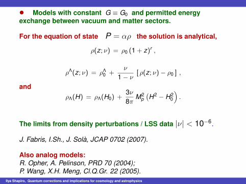
• Models with constant G ≡ G0 and permitted energyexchange between vacuum and matter sectors.
For the equation of state P = αρ the solution is analytical,
ρ(z; ν) = ρ0 (1 + z)r ,
ρΛ(z; ν) = ρΛ0 +ν
1 − ν[ ρ(z; ν)− ρ0 ] ,
andρΛ(H) = ρΛ(H0) +
3ν8π
M2p(H2 − H2
0
).
The limits from density perturbations / LSS data |ν| < 10−6.
J. Fabris, I.Sh., J. Solà, JCAP 0702 (2007).
Also analog models:R. Opher, A. Pelinson, PRD 70 (2004);P. Wang, X.H. Meng, Cl.Q.Gr. 22 (2005).
Ilya Shapiro, Quantum corrections and implications for cosmology and astrophysics

How to perturb a model with variable ρΛ = ρΛ(H) ?
ρt = ρm + ρΛ , PΛ = −ρΛ , Pm = 0 .
Introduce Uα. In the co-moving coordinates U0 = 1 andU i = Ui = 0.
T νµ =
(ρt + Pt
)UνUµ − Pt δ
νµ ,
such that T 00 = ρt and T j
i = −Pt δji .
Let us derive the covariant derivative of Uµ
∇µUµ = 3H .
The last equation enables one to perturb the running CC.
ρΛ = A + B(∇µUµ
)2,
where
A = ρ0Λ − 3 ν
8πM2
P H20 , B =
ν M2P
24π.
Ilya Shapiro, Quantum corrections and implications for cosmology and astrophysics

Final form of the perturbations equations
v ′ +(3f1 − 5)
1 + zv − k2ϱ(1 + z)
Hf1v = −k2ϱ(1 + z)
2Hh;
h′ +2(ν − 1)
1 + zh =
2 ν
(1 + z)
(2 vf1
− f1δm
ϱ
);
δ′m+
(f ′1f1
− 3f21 + z
)δm =
1f1
(ϱ h2
− ϱ vf1
)′
+1
1 + z
(3ϱ− 1
H
) (h2− v
f1
),
where (f1, f2) =(ρm
ρt,ρΛρt
), f (x , t) =
∫d3k(2π)3 f (k , t) ei k ·x .
v = f1∇i(δU i), h ≡ ∂
∂t
(hii
a2
), δρm = ρmδm
Given the Harrison-Zeldovich initial spectrum, the powerspectrum today can be obtained by integrating this system.
Initial data based on w(z) from J.M. Bardeen et al, Astr.J. (1986).Ilya Shapiro, Quantum corrections and implications for cosmology and astrophysics
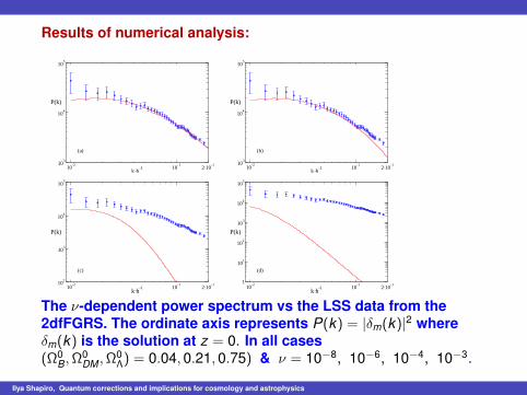
Results of numerical analysis:
10-2
10-1
2·10-1
k·h-1
103
104
105
P(k)
(a)
10-2
10-1
2·10-1
k·h-1
103
104
105
P(k)
(b)
10-2
10-1
2·10-1
k·h-1
102
103
104
105
P(k)
(c)
10-2
10-1
2·10-1
k·h-1
1
101
102
103
104
105
P(k)
(d)
The ν-dependent power spectrum vs the LSS data from the2dfFGRS. The ordinate axis represents P(k) = |δm(k)|2 whereδm(k) is the solution at z = 0. In all cases(Ω0
B,Ω0DM ,Ω0
Λ) = 0.04, 0.21, 0.75) & ν = 10−8, 10−6, 10−4, 10−3.
Ilya Shapiro, Quantum corrections and implications for cosmology and astrophysics
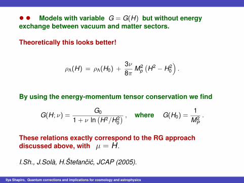
• • Models with variable G = G(H) but without energyexchange between vacuum and matter sectors.
Theoretically this looks better!
ρΛ(H) = ρΛ(H0) +3ν8π
M2p(H2 − H2
0
).
By using the energy-momentum tensor conservation we find
G(H; ν) =G0
1 + ν ln(H2/H2
0
) , where G(H0) =1
M2P.
These relations exactly correspond to the RG approachdiscussed above, with µ = H .
I.Sh., J.Solà, H.Štefancic, JCAP (2005).
Ilya Shapiro, Quantum corrections and implications for cosmology and astrophysics

The limits on ν from density perturbations
J.Grande, J.Solà, J.Fabris & I.Sh., Cl. Q. Grav. 27 (2010) .
An important general result is: In the models with variable Λand G in which matter is covariantly conserved, the solutionsof perturbation equations do not depend on the wavenumber k .
˙h + 2Hh = 8π[ρm − 2ρΛ
]δG + 8πG
[δρm − 2δρΛ
];
δρm + ρm
(θ − h
2
)+ 3Hδρm = 0 ;
θ + 2Hθ = 0 ;
δG(ρm + ρΛ) + δGρΛ + G(δρm + δρΛ) + GδρΛ = 0 ;
k2 [GδρΛ + ρΛδG] + a2ρmGθ = 0 .
Ilya Shapiro, Quantum corrections and implications for cosmology and astrophysics
As a consequence we meet relatively weak modifications of thespectrum compared to ΛCDM.
In our case the bound ν < 10−3 comes just from the “F-test”
R. Opher & A. Pelinson, astro-ph/0703779.J.Grande, R.Opher, A.Pelinson, J.Solà, JCAP 0712 (2007)
It is related only to the modification of the function H(z) .
One can obtain the same restriction for ν also from theprimordial nucleosynthesis (BBN).
Ilya Shapiro, Quantum corrections and implications for cosmology and astrophysics

Can we apply the running G(µ) to other physical problems?
In the renormalization group framework the relation
G(µ) =G0
1 + ν ln(µ2/µ2
0
) , where µ = H
in the cosmological setting.
What could be an interpretation of µ in astrophysics?
Consider the rotation curves of galaxies. The simplestassumption is µ ∝ 1/r .
Applications for the point-like model of galaxy:
J.T.Goldman, J.Perez-Mercader, F.Cooper & M.M.Nieto, PLB (1992).O. Bertolami, J.M. Mourao & J. Perez-Mercader, PLB 311 (1993).M. Reuter & H. Weyer, PRD 70 (2004); JCAP 0412 (2004).I.Sh., J.Solà, H.Štefancic, JCAP (2005).
Ilya Shapiro, Quantum corrections and implications for cosmology and astrophysics
We can safely restrict the consideration by a weakly varying G,
G = G0 + δG = G0(1 + κ) , |κ| ≪ 1 .
We already know that the appropriate value of the parameter ν issmall, the same should be with κ = δG/G0.
In order to link the metric in the variable G case with thestandard one, perform a conformal transformation
gµν =G0
Ggµν = (1 − κ)gµν .
Up to the higher orders in κ, the metric gµν satisfies usualEinstein equations with constant G0.
The nonrelativistic limits of the two metrics
g00 = −1 − 2Φc2 and g00 = −1 − 2ΦNewt
c2 ,
where ΦNewt is the usual Newton potential and Φ is a potential ofthe modifies gravitational theory.
Ilya Shapiro, Quantum corrections and implications for cosmology and astrophysics
We have
g00 = −1 − 2Φc2 = (1 + κ)g00
= (1 + κ)(−1 − 2ΦNewt
c2 ) ≈ −1 − 2ΦNewt
c2 − κ
and, hence,
Φ = ΦNewt +c2
2κ = ΦNewt +
c2 δG2 G0
.
For the nonrelativistic limit of the modified gravitational force weobtain, therefore,
−Φ,i = −Φ,iNewt −
c2 G,i
2 G0,
where we used the relation G,i = (δG),i .
Ilya Shapiro, Quantum corrections and implications for cosmology and astrophysics

The last formula
−Φ,i = −Φ,iNewt −
c2 G,i
2 G0= −Φ,i
Newt −c2
2κ,i ,
is indeed very instructive.
• Quantum correction comes multiplied by c2 =⇒ it does notneed being large to make real effect at the typical galaxy scale.
E.g., for a point-like model of galaxy and µ ∝ 1/r it issufficient to have ν ≈ 10−6 to provide flat rotation curves.
I.Sh., J.Solà, H.Štefancic, JCAP (2005).
•• µ ∝ 1/r is, obviously, not a really good choice for anon-point-like model of the galaxy.
The reason is that this identification produces the“quantum-gravitational” force even if there is no mass at all !!
Ilya Shapiro, Quantum corrections and implications for cosmology and astrophysics
What would be the “right” identification of the renormalizationgroup scale parameter µ in the quase-Newtonian regime?
Let us come back to the quantum field theory (QFT). We arecurrently unable to derive quantum corrections to the GR action.
At the same time the QFT gives us a good hint:µ must be accociated to some parameter which characterizesthe energy of the particle corresponding to the externalgravitational line in the Feynman diagram.
Of course, µ ∝ 1/r is not not the right choice.
Ilya Shapiro, Quantum corrections and implications for cosmology and astrophysics
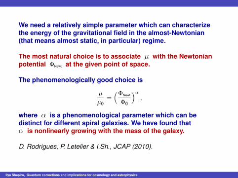
We need a relatively simple parameter which can characterizethe energy of the gravitational field in the almost-Newtonian(that means almost static, in particular) regime.
The most natural choice is to associate µ with the Newtonianpotential ΦNewt at the given point of space.
The phenomenologically good choice is
µ
µ0=(ΦNewt
Φ0
)α,
where α is a phenomenological parameter which can bedistinct for different spiral galaxies. We have found thatα is nonlinearly growing with the mass of the galaxy.
D. Rodrigues, P. Letelier & I.Sh., JCAP (2010).
Ilya Shapiro, Quantum corrections and implications for cosmology and astrophysics

Definitely, α is a “good guy” in this story.
From the QFT viewpoint the presence of α reflects the fact thatthe association of µ with ΦNewt is not an ultimate choice.Remember the vacuum EA is a relativistic object and taking ΦNewt
as a scale definitely ignores some relevant information.
With greater mass of the galaxy the “error” in identificationbecomes greater too, hence we need a greater α to correct this.Furthermore, if α increases with the mass of the galaxy, it mustbe very small at the scale of the Sun system and of course at thescale of laboratory, when the Newton law is better verified.
Remarkably, the recently-proposed regular scale-settingprocedure gives the very same result:
S. Domazet, H.Štefancic, PLB (2011) - in press.
Ilya Shapiro, Quantum corrections and implications for cosmology and astrophysics
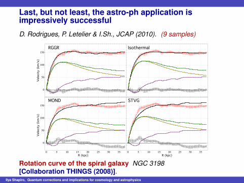
Last, but not least, the astro-ph application isimpressively successful
D. Rodrigues, P. Letelier & I.Sh., JCAP (2010). (9 samples)
!
!
!
!
!
!
!
!
!
!
!
!
!
!!!!!!
!!!!!!!!! !!!!!!!!
!!!!!!!!!!
!!!!!!!!!!!!!!!!!!!!!! !!!!!!!!!!!
!!!!!!! !!!!!!!
!
" "" """"
""""
""" ""
""""""""""""
""""" """""""""" """"""" ""
"""" """""""""""" "
"" "" "" """ "" """""" ""
""" """
0 5 10 15 20 25 30 35
0
50
100
150
!
!
!
!
!
!
!
!
!
!
!
!
!
!!!!!!
!!!!!!!!! !!!!!!!!
!!!!!!!!!!
!!!!!!!!!!!!!!!!!!!!!! !!!!!!!!!!!
!!!!!!! !!!!!!!
!
"""""""""
""
""" ""
""""""
"""""
""""""
""""""""
"" """"
""" """""" """"""
"""""" """ "" "" """ "
" """""" ""
""" """
0
50
100
150
!
!
!
!
!
!
!
!
!
!
!
!
!
!!!!!!
!!!!!!!!! !!!!!!!!
!!!!!!!!!!
!!!!!!!!!!!!!!!!!!!!!! !!!!!!!!!!!
!!!!!!! !!!!!!!
!
""" """""
"""
""" ""
"""""""""""" """"" ""
"""""""" """"""" ""
"""" """""""""""" "
"" "" "" """"" """
""" """"" """
0 5 10 15 20 25 30 35
!
!
!
!
!
!
!
!
!
!
!
!
!
!!!!!!
!!!!!!!!! !!!!!!!!
!!!!!!!!!!
!!!!!!!!!!!!!!!!!!!!!! !!!!!!!!!!!
!!!!!!! !!!!!!!
!
" """"""""
""
""" ""
"""""""
""""""""""
""""""""""
""""""" """""" """""""""""" """ "" "" """ "
" """""" """"" ""
"
Velocity (km/s)
Velocity (km/s)
R (kpc) R (kpc)
RGGR Isothermal
MOND STVG
Rotation curve of the spiral galaxy NGC 3198[Collaboration THINGS (2008)].
Ilya Shapiro, Quantum corrections and implications for cosmology and astrophysics
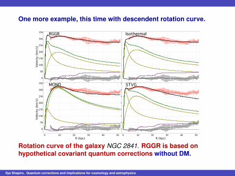
One more example, this time with descendent rotation curve.
!!!!!!!!!!! !! !!!!!!!!!!!!!!!!!!!!!
!
!!!!!!!!!!!!!!!!!!!!!!!!!!!!!!!!!!!!!!!!!!!!!
!!!!!!!!!!!!!!!!!!!!!!!!!!!!!!!!!!!!!!
!!!!!!!!
!!!!!!!!!
!!!
!!!
""""""""""" "" """"""
"""""""""""""""
"
"""""""""""""
""""""
""""""""""""""""""
"""""""
"""""""
""""""""""""""""""""""""""""""""""""""""
"""""""""
"""
"""
0 10 20 30 40 50
0
50
100
150
200
250
300
350
!!!!!!!!!!! !! !!!!!!!!!!!!!!!!!!!!!
!
!!!!!!!!!!!!!!!!!!!!!!!!!!!!!!!!!!!!!!!!!!!!!
!!!!!!!!!!!!!!!!!!!!!!!!!!!!!!!!!!!!!!
!!!!!!!!
!!!!!!!!!
!!!
!!!
""""""""""
" "" """""""""""""""""""""
"
""""""""""""""""""""""""
""""""""""""""""""""
"""""""
""""""""""""""""""""""""""""""""""""""""
"""""""""
"""
"""
0
50
100
150
200
250
300
350
!!!!!!!!!!! !! !!!!!!!!!!!!!!!!!!!!!
!
!!!!!!!!!!!!!!!!!!!!!!!!!!!!!!!!!!!!!!!!!!!!!
!!!!!!!!!!!!!!!!!!!!!!!!!!!!!!!!!!!!!!
!!!!!!!!
!!!!!!!!!
!!!
!!!
""""""""""" "" """""""""""""
"""""""""
"""""""""""""""""""
""""""""""""""""""
"""""""
"""""""
""""""""""""""""""""""""""""""""""""""""
"""""""""
"""
"""
!!!!!!!!!!! !! !!!!!!!!!!!!!!!!!!!!!
!
!!!!!!!!!!!!!!!!!!!!!!!!!!!!!!!!!!!!!!!!!!!!!
!!!!!!!!!!!!!!!!!!!!!!!!!!!!!!!!!!!!!!
!!!!!!!!
!!!!!!!!!
!!!
!!!
""""""""""" "" """"""""""""""
"""""""
"
""""""""""""""""""""
""""""""""
"""""""""
"""""""""""
""""""""""""""""""""""
"""""""""""""""""""
""""""""""""
"""
0 10 20 30 40 50
0
50
100
150
200
250
300
350
Velocity (km/s)
Velocity (km/s)
R (kpc) R (kpc)
RGGR Isothermal
MOND STVG
Rotation curve of the galaxy NGC 2841. RGGR is based onhypothetical covariant quantum corrections without DM.
Ilya Shapiro, Quantum corrections and implications for cosmology and astrophysics
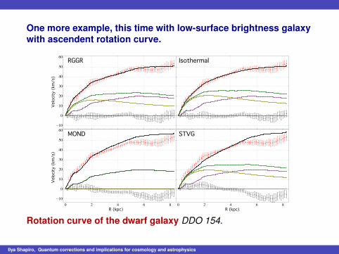
One more example, this time with low-surface brightness galaxywith ascendent rotation curve.
!
!
!
!!!
!
!
!
!
!
!
!
!! !
!!!!!!!! !
!!!!!!!!!!! ! ! ! ! ! !
! !! ! ! ! !
! !! !
!!
!
!!
!!!
"
" """ "
"" "
" " """ "
"" " " "
" " " " " " " " " " " " " " " " "
"" "
" " " """"" "
" "" "
""
"
""
"" "
0 2 4 6 8
!10
0
10
20
30
40
50
60
!
!
!
!!!
!
!
!
!
!
!
!
!! !
!!!!!!!! !
!!!!!!!!!!! ! ! ! ! ! !
! !! ! ! ! !
! !! !
!!
!
!!
!!!
"
" ""
"""" " "
"" " " "
" " " " " " " " " " """ " " "
" " " "" "
"" "
" "" "
"""" "
" "" "
""
"
""
"" "
!10
0
10
20
30
40
50
60
!
!
!
!!!
!
!
!
!
!
!
!
!! !
!!!!!!!! !
!!!!!!!!!!! ! ! ! ! ! !
! !! ! ! ! !
! !! !
!!
!
!!
!!!
"
"" "
""""" " "
" " " """ " " "
" " " " " " " " " " " " " " " " "
"" "
"" " "
"""" "
" "
" """
"
"""" "
0 2 4 6 8
!
!
!
!!!
!
!
!
!
!
!
!
!! !
!!!!!!!! !
!!!!!!!!!!! ! ! ! ! ! !
! !! ! ! ! !
! !! !
!!
!
!!
!!!
"
"" "
"" "
" " " "" " " "
" " " " " " " " " " " "" "
" " "" " "
" """ " " " " "
"" "
" "" "
" "" "
"
""
"" "
Velocity (km/s)
Velocity (km/s)
R (kpc) R (kpc)
RGGR Isothermal
MOND STVG
Rotation curve of the dwarf galaxy DDO 154.
Ilya Shapiro, Quantum corrections and implications for cosmology and astrophysics
What about the Solar System?
C. Farina, W. Kort-Kamp, S. Mauro, I.Sh., PRD 83 (2011).
We used the dynamics of the Laplace-Runge-Lenz vector in theG(µ) = G0/(1 + µ log(µ/µ0)) - corrected Newton gravity.
Upper bound for the Solar System: αν ≤ 10−17.
One of the works now on track: extending the galaxies sample.
P. Louzada, D. Rodrigues, J. Fabris, ..., in work: 50+ disk galaxies.
D. Rodrigues, N. Napolitano, ..., in progress: elliptical galaxies.
The general tendency which we observe so far is greater αneeded to for larger mass of the astrophysical object: fromSolar System (upper bound) to biggest tested galaxies.
Ilya Shapiro, Quantum corrections and implications for cosmology and astrophysics
It looks like we do not need CDM to explain the rotation curvesof the galaxies. However, does it really mean that we can reallygo on with one less dark component?
Maybe not, but it is worthwhile to check it. It is well known thatthe main requests for the DM come from the fitting of the LSS,CMB, BAO, lenthing etc.
However there is certain hope to relpace, e.g., ΛCDM by aΛWDM (e.g. sterile neutrino) with much smaller ΩDM .
The idea to trade 0.04, 0.23, 0.73 =⇒ 0.04, 0.0x, 0.9(1-x)
Such a new concordance model would have less relevantcoincidence problem, and in general such a possibility isinteresting to verify.
First move:J. Fabris, A. Toribio & I.Sh., Testing DM warmness and quantity viathe RRG model. arXiv:1105.2275 [astro-ph.CO]
We are using “our” Reduced Relativistic Gas model.Ilya Shapiro, Quantum corrections and implications for cosmology and astrophysics
The Reduced Relativistic Gas model is a Simple cosmologicalmodel with relativistic gas.
G. de Berredo-Peixoto, I.Sh., F. Sobreira, Mod.Ph.Lett. A (2005);J. Fabris, I.Sh., F.Sobreira, JCAP (2009).
The model describes ideal gas of massive relativistic particleswith all of them have the same kinetic energy.
The Equation of State (EOS) of such gas is
P =ρ
3
[1 −
(mc2
ε
)]2=
ρ
3
(1 −
ρ2d
ρ2
).
In this formula ε is the kinetic energy of the individual particle,ε = mc2/
√1 − β2. Furthermore, ρd = ρ2
d0(1 + z)3 is the mass(static energy) density. One can use one or another form of theequation of state (1), depending on the situation.
Ilya Shapiro, Quantum corrections and implications for cosmology and astrophysics

The nice thing is that one can solve the Friedmann equation inthis model analytically. The deviation from Maxwell or relativisticFermi-Dirac distribution is less than 2.5%.
The model was sucessfully used to impose the upper bound tothe warmness of DM from LSS data, providing the same resultsas more complicated models.
J. Fabris, I.Sh., F.Sobreira, JCAP (2009). DM particles: how warmthey can be?
So, why it is “our” and not just our model?
Because we were not first. The same EOS has been used byA.D. Sakharov in 1965. to predict the oscillations in the CMBspectrum for the first time!!
A.D. Sakharov, Soviet Physics JETP, 49 (1965) , 345.
Ilya Shapiro, Quantum corrections and implications for cosmology and astrophysics

In the recent preprint (under consideration in PRD)
J. Fabris, A. Toribio & I.Sh., Testing DM warmness and quantity viathe RRG model. arXiv:1105.2275 [astro-ph.CO]
we have used RRG without quantum effects to fitSupernova type Ia (Union2 sample), H(z), CMB (R factor),BAO, LSS (2dfGRS data)In this way we confirm that ΛCDM is the most favored model.
However, for the LSS data alone we met the possibility of analternative model with a small quantity of a WDM.
This output is potentially relevant in view of the fact that the LSSis the only test which can not be affected by the possiblequantum renormalization-group running in the low-energygravitational action.
Ilya Shapiro, Quantum corrections and implications for cosmology and astrophysics
Conclusions
• The evaluation of quantum corrections from massive fields is,to some extent, reduced to existing-nonexisting paradigm.
• In the positive case we arrive at the cosmological andastrophysical model with one free parameter ν plus certainfreedom of scale identification.
• The rotation curves of all tested galaxies can be described bythe G(µ) formula. The situation with clasters and other tests,especially CMB and lensing, remains unclear.
• The power spectrum tests are less sensible to the G(µ) andexactly in this case we meet an alternative to ΛCDM in thezero-order approximation.
• Finally, there is still some (albeit small) chance that thevacuum effects of QFT in an external gravitational field playmore significant role in our Universe that we use to imagine.
Ilya Shapiro, Quantum corrections and implications for cosmology and astrophysics