Khalid Eid

Quantized Conductance: An

Advanced Lab About the

Wave Nature of Matter

Department of Physics

Miami University

Oxford, Ohio

All Rights Reserved by the Author Summer 2015

CONTENTS

INTRODUCTION: .......................................................................................................................... 8

OVERVIEW OF SETUP AND WORKSHOP ACTIVITIES ........................................................... 9

PREPARING BENDING BEAMS, WIRES, AND EPOXY DROPS .............................................. 12

SETUP ASSEMBLY, CUTTING WIRES, AND PROGRAM ........................................................ 13

FIRST LABVIEW MEASUREMNTS OF RESISTANCE .............................................................. 15

WAYS TO DISCUSS THE EXPERIMENT IN A CLASSROOM ................................................... 17

FURTHER WORK AND DATA ANALYSIS ................................................................................ 18

CONTROLLING THE MICROMETER WITH A PIEZO-CRYSTAL ........................................... 20 PURCHASE LIST FOR SETUP …………………………………………………………………………………… 23

INTRODUCTION

Quantum mechanics dominates the atomic and sub-atomic world, but it quickly

approaches the classical limit in systems with high energy or large dimensions (relative to

the atomic scale). So, the typical experiments to study quantum mechanics are

spectroscopy-based and study atoms, molecules or nulcei.

The quantized conductance in gold wires that are stretched and are just about to break

offers a very different approach to demonstrate quantum mechanical behavior. It is based

on transport (i.e. current-voltage) measurements. Furthermore, the students can see all

components of the setup with their own naked eyes and the setup is manually controlled to

break the gold wire and reconnect it. As the gold wire gets so thin that its diameter is

comparable to the de Broglei wavelength of the electrons that carry the electric charge,

these electron waves ‘start to feel’ the boundaries of the wire and only certain states

become available for these electrons to occupy and travel through. This is a typical

quantum mechanical behavior, just like the quantization of energy levels, wavelengths, and

momenta that are allowed for an electron in an infinite potential well. This makes the

quantized conductance a nice experiment or demonstration of the applicability of infinite

potential well concepts in real applications. These quantized conductance values are always

multiples of an integer number times a combination of two universal constants in nature;

the electron charge and the Plank constant. An important practical point about the setup is

that gold does not oxidyze, so a broken gold wire will readily reconnect and merge back as

soon as the two ends are brought back into contact. So, the experiment can be done many

times on the same wire and the wire can stay good for years.

The main objectives of the quantized conductance (QC) experiment are:

1. To demonstrate the emergence of quantized conductance as a gold wire is broken and

reconnected.

2. To find the value of the quantized conductance from experimental data.

3. To link the QC with wave-particle duality and to demonstrate that confinement/boundary

conditions gives rise to quantization.

4. To link the shape of the conductance curve with the correspondence principle.

5. To understand the size scales at which different scattering phenomena occur in solids.

SUMMER 2014 3

A major challenge for achieving this quantized behavior is the control of the break junction or the constriction area at the atomic scale! Different equipment are used to achieve that in research

lab, yet the cost and the complexity of the setup make it harder to get and of less pedagogical value to help the students appreciate the science. The setup used in this workshop combines the

required atomic control of the stretching of the gold wire, the low cost, and the simplicity that make it of excellent value in a teaching laboratory or lecture demonstration.

OVERVIEW OF EXPERIMENTAL SETUP AND ACTIVITIES

This mechanically-controlled break junction (MCBJ) setup uses a spring steel sheet as a bending

beam and a micrometer to stretch a 99.99% purity, 3.5”-long and 75µm-wide gold wire with

atomic displacement accuracy. The SM-25 Vernier Micrometer has a resolution of about 1µm

and is rotated manually by attaching it to a plastic disc of radius 5”. The 1095 Blue Tempered

Spring Steel sheet is a little over 3” long, 0.5” wide, and 0.008” in thickness. The barrel of the

micrometer passes through a hole in an aluminum housing block and is secured by a set screw.

When fully retracted, the micrometer head is flush with the aluminum block. Two stops are

placed 3” apart, centered on the hole for the micrometer head. These conductive stops are

electrically insulated from the main aluminum block by a length of plastic tubing. These stops

are positioned so that there is 4mm of distance between the fully retracted micrometer head and

the plane of the stops. The sample is placed in this space, and the micrometer head is advanced to

make contact with the sample. With the barrel of the micrometer secured in place, the tip can be

extended and retracted by rotating the thimble. As the tip extends, it presses into the middle of

the spring steel sheet. This bends the spring steel outwards against the two stops, producing the

desired bending motion. If the sample is particularly long, as it bends the ends of the spring steel

sheet may contact the aluminum block. This is prevented by cutting two clearance notches on

either side of the block. Fig. 1 shows the setup used in this experiment.

Since the spring steel sheet is conductive, we need to paste a cigarette paper on it, and then attach

the gold wire using two droplets of Double/Bubble insulating epoxy with a narrow gap between

them as shown in Fig. 1c). After the epoxy hardens, we use a sharp blade to cut a shallow notch

in the gold wire. The blade is also used to cut a groove in the epoxy if the two droplets merge

together. Fig. 1d) is a scanning electron microscope image of the partly cut wire and the two

epoxy drops.

Fig. 1. Pictures of the MCBJ setup. a) The MCBJ assembly showing the pin of the micrometer, the bending beam, the stops and the wire. No solder is needed to connect the ends of the gold

wire to the stops. b) The experimental setup showing the plastic disk used to rotate the micrometer, the battery and wires, as well as the bending beam. c) A gold wire mounted on a

sheet of spring steel and a quarter dollar coin is placed next to it for visual comparison. The two epoxy drops are seen in the middle. d) Scanning electron microscope image of the wire and the two drops. The wire is partially cut in the middle to create a week point in it.

When turning the plastic disk and micrometer, the wire stretches extremely slowly with a

reduction factor (f) given by: 𝑓 = 3𝑦𝑠

𝑢2 , where y is the distance between the two epoxy drops, s

the thickness of the spring steel sheet and the insulating film, and u is the separation between the

two stopping edges. We estimate that f ~ 2 x 10-5 (corresponding to a mechanical reduction of

50,000), which gives atomic scale motion, when multiplied by the micrometer resolution of 1µm.

The huge reduction in the bending beam is the key to achieve atomic scale motion and to

eliminate the effect of external vibrations on the experiment. The current through the constriction

is produced by connecting the wire in series to an external resistor of 100KΩ and a 1.5V battery.

As the wire is pulled, the voltage across it is measured repeatedly at a high rate (10,000 samples

per second) using a National Instruments data acquisition (DAQ) unit and a simple LabVIEW

program. The circuit diagram and the LabVIEW program used to collect the data are shown in

Fig. 2.

SUMMER 2014 5

Fig. 2. a) A simple electrical circuit is used to measure the conductance of the gold wire and b) a

very basic LabVIEW program monitors and records the data

SAMPLE PREP: BENDING BEAM, GOLD WIRE & EPOXY DROPS

Objectives:

1- To Cut the proper length of bending beam and use cigarette paper to make it

insulating

2- To place two epoxy drops, with the proper size and shape, spaced < 0.5mm from

each other and placed over the mid part of the gold wire

The steps to prepare the gold wires that are attached to the ‘insulating’ bending beam

(shown in Fig. 1(c) and the pictures below) as follows:

1- Use a shear cutter to cut 5 sheets of springy steel to a length of about 3”.

2- Mix the two components of a small bag of ‘Very-high Peel Strength’

Double/Bubble epoxy, and then divide that into three smaller amounts for each

participant to have enough to prepare their samples.

3- Use scissors to cut 5, ¼”-wide sheets from a cigarette paper (cut along the long

side of the cigarette paper).

4- Spread 3 to 5 small drops of epoxy along the middle of the springy steel (roughly

along the long axis that goes through the center of the sheet).

5- Lay a ¼” cigarette paper piece over each springy steel sheet and smooth it out by

gently pressing with your fingertips. Prepare Five of these ‘bending beam

assemblies’.

6- Since the cigarette paper is shorter than the spring steel sheet, use scotch tape to

cover the two far ends of the SS sheet to electrically isolate them.

7- Cut five 75-micrometer Gold wires to a length of ~3.5”.

8- To attach a gold wire on a cigarette-paper-covered spring steel sheet: Gently

stretch the wire with your hands to make it less ‘wrinkly’. Place the gold wire

over the attached cigarette paper such that the middle of the wire roughly sits on

the middle of the bending beam.

9- It is important to keep the gold wire slightly tight/snug during and after the

placement of the two epoxy drops. This can be achieved with a small amount of

scotch tape.

10- Use a pair of tweezers to gently press on the wire to keep it in place and use your

dominant hand to place a drop of the mixed epoxy just to the side of the middle

section of the wire.

11- A good way to place the droplets is to let the droplet touch the wire/cigarette

paper, and then pull the droplet away from the center and along the gold wire.

This ensures that the droplet will not be two large or two high above the wire.

12- Place a second epoxy drop about 0.5mm away from the first drop such that the

gap is at the center of the wire. Again, try to pull the drop away from the center.

SUMMER 2014 7

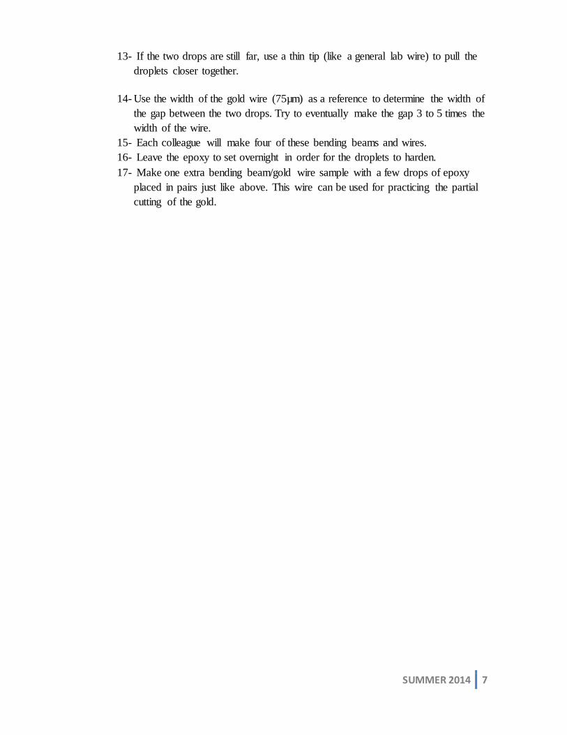
13- If the two drops are still far, use a thin tip (like a general lab wire) to pull the

droplets closer together.

14- Use the width of the gold wire (75µm) as a reference to determine the width of

the gap between the two drops. Try to eventually make the gap 3 to 5 times the

width of the wire.

15- Each colleague will make four of these bending beams and wires.

16- Leave the epoxy to set overnight in order for the droplets to harden.

17- Make one extra bending beam/gold wire sample with a few drops of epoxy

placed in pairs just like above. This wire can be used for practicing the partial

cutting of the gold.

Sample preparation pictures

SUMMER 2014 9

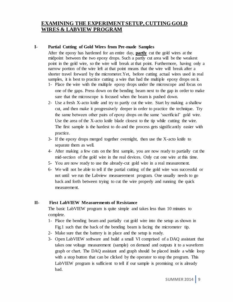
EXAMINING THE EXPERIMENT SETUP, CUTTING GOLD WIRES & LABVIEW PROGRAM

I- Partial Cutting of Gold Wires from Pre-made Samples

After the epoxy has hardened for an entire day, partly cut the gold wires at the midpoint between the two epoxy drops. Such a partly cut area will be the weakest

point in the gold wire, so the wire will break at that point. Furthermore, having only a narrow portion of the wire left at that point means that the wire will break after a

shorter travel forward by the micrometer.Yet, before cutting actual wires used in real samples, it is best to practice cutting a wire that had the multiple epoxy drops on it. 1- Place the wire with the multiple epoxy drops under the microscope and focus on

one of the gaps. Press down on the bending beam next to the gap in order to make

sure that the microscope is focused when the beam is pushed down.

2- Use a fresh X-acto knife and try to partly cut the wire. Start by making a shallow

cut, and then make it progressively deeper in order to practice the technique. Try

the same between other pairs of epoxy drops on the same ‘sacrificial’ gold wire.

Use the area of the X-acto knife blade closest to the tip while cutting the wire.

The first sample is the hardest to do and the process gets significantly easier with

practice.

3- If the epoxy drops merged together overnight, then use the X-acto knife to

separate them as well.

4- After making a few cuts on the first sample, you are now ready to partially cut the

mid-section of the gold wire in the real devices. Only cut one wire at this time.

5- You are now ready to use the already-cut gold wire in a real measurement.

6- We will not be able to tell if the partial cutting of the gold wire was successful or

not until we run the Labview measuerement program. One usually needs to go

back and forth between trying to cut the wire properly and running the quick

measurement.

II- First LabVIEW Measurements of Resistance

The basic LabVIEW program is quite simple and takes less than 10 minutes to

complete.

1- Place the bending beam and partially cut gold wire into the setup as shown in

Fig.1 such that the back of the bending beam is facing the micrometer tip.

2- Make sure that the battery is in place and the setup is ready.

3- Open LabVIEW software and build a small VI comprised of a DAQ assistant that

takes one voltage measurement (sample) on demand and outputs it to a waveform

graph or chart. The DAQ assistant and graph should be placed inside a while loop

with a stop button that can be clicked by the operator to stop the program. This

LabVIEW program is sufficient to tell if our sample is promising or is already

bad.

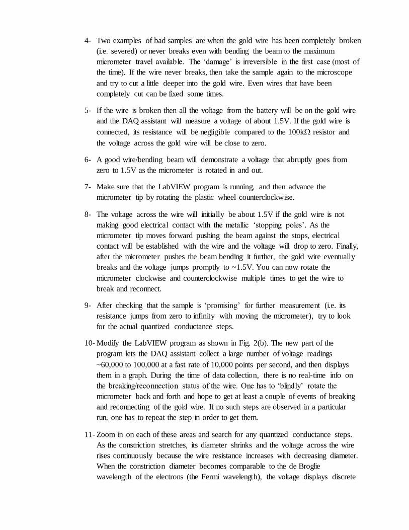
4- Two examples of bad samples are when the gold wire has been completely broken

(i.e. severed) or never breaks even with bending the beam to the maximum

micrometer travel available. The ‘damage’ is irreversible in the first case (most of

the time). If the wire never breaks, then take the sample again to the microscope

and try to cut a little deeper into the gold wire. Even wires that have been

completely cut can be fixed some times.

5- If the wire is broken then all the voltage from the battery will be on the gold wire

and the DAQ assistant will measure a voltage of about 1.5V. If the gold wire is

connected, its resistance will be negligible compared to the 100k resistor and

the voltage across the gold wire will be close to zero.

6- A good wire/bending beam will demonstrate a voltage that abruptly goes from

zero to 1.5V as the micrometer is rotated in and out.

7- Make sure that the LabVIEW program is running, and then advance the

micrometer tip by rotating the plastic wheel counterclockwise.

8- The voltage across the wire will initially be about 1.5V if the gold wire is not

making good electrical contact with the metallic ‘stopping poles’. As the

micrometer tip moves forward pushing the beam against the stops, electrical

contact will be established with the wire and the voltage will drop to zero. Finally,

after the micrometer pushes the beam bending it further, the gold wire eventually

breaks and the voltage jumps promptly to ~1.5V. You can now rotate the

micrometer clockwise and counterclockwise multiple times to get the wire to

break and reconnect.

9- After checking that the sample is ‘promising’ for further measurement (i.e. its

resistance jumps from zero to infinity with moving the micrometer), try to look

for the actual quantized conductance steps.

10- Modify the LabVIEW program as shown in Fig. 2(b). The new part of the

program lets the DAQ assistant collect a large number of voltage readings

~60,000 to 100,000 at a fast rate of 10,000 points per second, and then displays

them in a graph. During the time of data collection, there is no real-time info on

the breaking/reconnection status of the wire. One has to ‘blindly’ rotate the

micrometer back and forth and hope to get at least a couple of events of breaking

and reconnecting of the gold wire. If no such steps are observed in a particular

run, one has to repeat the step in order to get them.

11- Zoom in on each of these areas and search for any quantized conductance steps.

As the constriction stretches, its diameter shrinks and the voltage across the wire

rises continuously because the wire resistance increases with decreasing diameter.

When the constriction diameter becomes comparable to the de Broglie

wavelength of the electrons (the Fermi wavelength), the voltage displays discrete

SUMMER 2014 11

steps rather than a smooth increase. Since the wire is connected in series to the

external resistor of 100kΩ, the voltage across the constriction is: Vw = IRw =VB

Rw+RextRw and the conductance is:

G =VB −Vw

Vw Rext (1)

Here, VB is the battery voltage, Rext is the external resistor, and Rw is the

resistance of the wire (i.e. the constriction).

To determine which steps correspond to an actual quantized conductance channel,

Equation (1) can then be combined with:

Gn = 2e2

hn (2)

12- Use Equs. 1 and 2 to modify an Excel sheet of the data such that it displays the

number of quantized channels on the y-axis, instead of voltage.

13- While the LabVIEW program and the analysis above are quite simple, it can be

confusing when trying to determine which conductance steps correspond to which

channel (i.e. quantum) number (n). Instead, modify the LabVIEW program to

build in the results of Equ.s (1) and (2) and plot (n) directly on the Y-axis of the

LabVIEW graph.

14- This is the simplest way to ‘read’ the results of a particular run.

15- You might need to collect several sets of data in order to get satisfactory

quantization results, as the steps do not occur in every run. Also, feel free to

change the sample if it does not give good results.

16- One can simply take a snapshot of the screen using “print screen” in order to

insert the results into a report, or better save the data as an Excel sheet for further

processing.

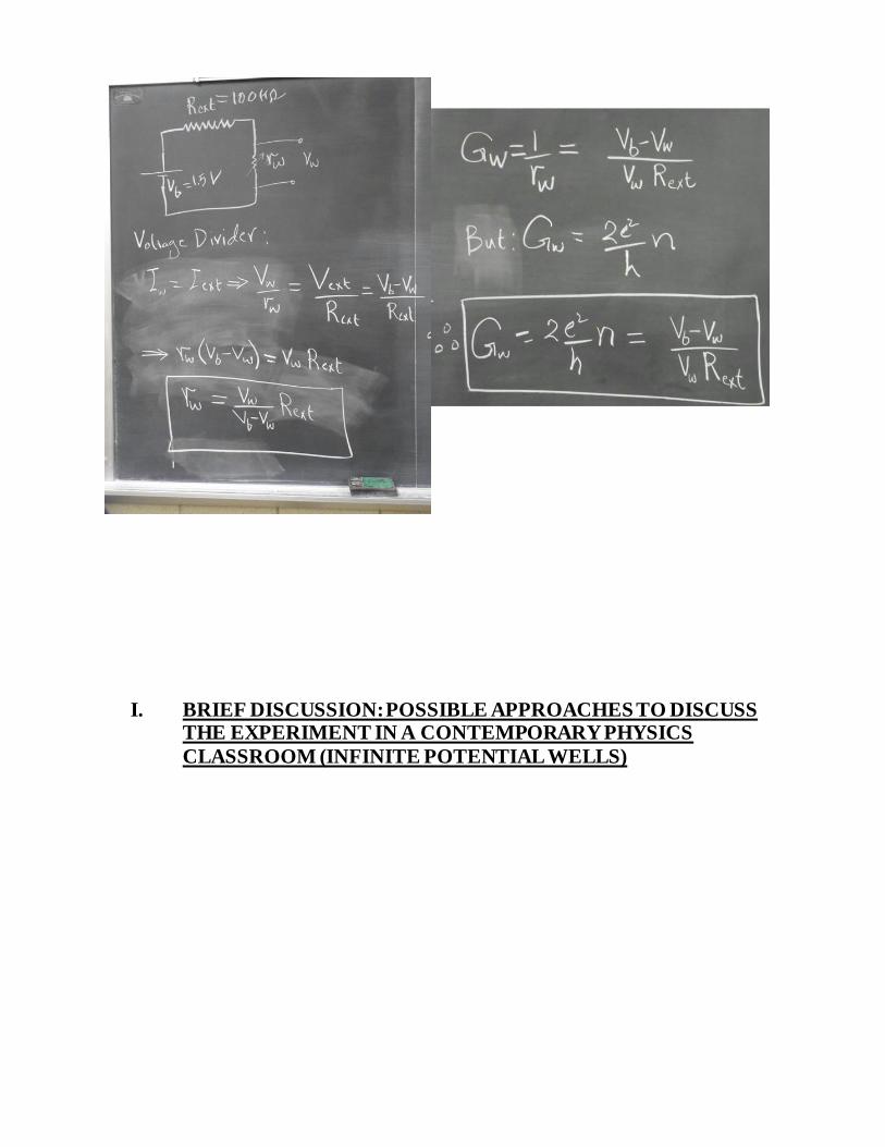
I. BRIEF DISCUSSION: POSSIBLE APPROACHES TO DISCUSS THE EXPERIMENT IN A CONTEMPORARY PHYSICS

CLASSROOM (INFINITE POTENTIAL WELLS)

SUMMER 2014 13

Fig. 3: As the width of the well gets smaller, the difference between energy levels

widen. So, less energy levels (i.e. eigen states) are allowed below the Fermi Energy, which is constant.

Important concepts for the discussion are: The Fermi energy, the infinite well-potentials, standing waves.

CONTROLLING THE MICROMETER USING A PIEZO-CRYSTAL

We will run the Quantized Conductance experiment using LabVIEW with a programmable

piezo-crystal and also using a manually driven piezo-crystal. The use of the piezo-crystals introduces noise in the measurements and tends to give less quality data than the manual operation. The fully manual operation gives the cleanest results and is the simplist to understand

easily. Yet, the Piezo crystals offer finer control over the breaking process, which means that the quantized steps will last for a longer time than in the fully manual operation.

I) LabVIEW and a programmable piezo-crystal

A ‘Piezo Jena’ piezo-crystal system will be used to collect a large number of data.

1- Change the head of the setup to incorporate the piezo-crystal and its electronics

and attach the micrometer to the setup.

2- The piezo-crystal setup comes programmed to work with LabVIEW. We will run

both that program and the program for data collection at the same time.

3- Manually rotate the micrometer to break and reconnect the gold wire several

times, and then stop as close as possible to the ‘breaking point’.

4- Run the Piezo Jena software and change the frequency to 0.1Hz and the amplitude

to 10%. These parameters define the frequency at which the crystal oscillates

between contracted and extended position and the percent of full extension

distance, respectively. You can also open a display that shows the status of the

crystal (how extended it is). Pick a triangular wave for the crystal. Try to change

the frequency and the amplitude and see what effect they have.

5- This setup can be used to collect a large number of data points and to ‘build’ a

histogram that shows the quantization and helps get rid of random noise. Yet, the

main limitation is the total number of data points that can be collected at any

given run.

References

1. Modern Physics textbook by Tippler and Llewellyn Chapter 10, sections 10.2 (Classical

conduction), 10.4 (Quantum Theory of Conduction), 10.6 (Band theory of solids).

2. R. Tolley, A. Silvidi, C. Little, K.F. Eid, Amer. J. Phys. 81, 14 (2013)

SUMMER 2014 15

PURCHASES LIST FOR SETUP

Here is a list of items to purchase for setting up the quantized conductance experiment:

1. Gold wire: We usually use a 0.0031” (i.e. 75 micrometer) gold wire that we bought from

California Fine Wire Company. I never tried thicker wires, but I imagine that they would be even

easier to handle. The website of the company is: http://www.calfinewire.com/

Price: $220 for our last purchase of a 50’ (Fifty foot) wire.

2. Blue-Finished and Polished 1095 Spring Steel

.008" Thick, 3/4" Width, 10' Coil (Part number at McMaster-Carr is: 9075K29). We tried a

thicker sheet, but it was much harder to bend and to handle.

Price $31 for our last purchase of 10’ sheet.

3. SM-25 Vernier Micrometer. http://www.newport.com/Vernier-Micrometer-Heads,-SM-

Series/140173/1033/info.aspx

Price: ~$105

4. DAQ Unit (NI USB-6009):

Price: $279 (48k samples/sec)

5. LabVIEW License: I do not know about the cost of the license; we have a site license.

6. Machine shop, glue, cigarette papers, X-acto knife and other materials: Depends on how

your machine shop charges, but the cost of the actual materials is ~ $50.

Conductance quantization: A laboratory experiment in a senior-levelnanoscale science and technology course

R. Tolley, A. Silvidi, C. Little, and K. F. Eida)

Department of Physics, Miami University, Oxford, Ohio 45056

(Received 13 March 2012; accepted 17 October 2012)

We describe a simple, inexpensive, and robust undergraduate lab experiment that demonstrates the

emergence of quantized conductance as a macroscopic gold wire is broken and unbroken. The

experiment utilizes a mechanically controlled break junction and demonstrates how conductance

quantization can be used to understand the importance of quantum mechanics at the nanoscale.

Such an experiment can be integrated into the curriculum of a course on nanoscale science or

contemporary physics at the junior and senior levels. VC 2013 American Association of Physics Teachers.

[http://dx.doi.org/10.1119/1.4765331]

I. INTRODUCTION

The past two decades have witnessed an enormous surgeof interest in nanotechnology and nanoscience. This interestis fueled by predictions that nanotechnology will have a sig-nificant and broad impact on many aspects of the future,including technology,1 food,2 medicine,3,4 and sustainableenergy.5 Many universities in the United States and aroundthe world began to establish programs teaching nanotechnol-ogy in order to produce the necessary nanoscale-skilledworkforce6–8 and to inform the public about nanotechnol-ogy’s potential benefits and environmental risks.9,10 Nano-scale science and technology programs have even beenutilized to sustain low-enrollment physics programs and toreform the Science, Technology, Engineering, and Mathe-matics (STEM) focus.11 However, it is necessary to deviseadditional experiments and to develop curricula that will mo-tivate the field properly and provide undergraduate studentswith a good appreciation and basic understanding of thenanoscale.12,13 Several core concepts have been identified asfundamental to student understanding of phenomena at thenanoscale.14 Two such concepts are the importance of quan-tum mechanics and the understanding of the sizes and scalesat which interesting phenomena occur. Quantum mechanicsshows that when matter is confined at the atomic scale, it canhave quantitatively and qualitatively different propertiesthan the macroscopic scale.15 One consequence of this con-finement and the particle-wave duality is the quantization ofelectrical conductance, where the classical electron transportproperties and the well-established Ohm’s Law cease toapply.16

We develop a simple, inexpensive, and robust laboratoryexperiment on conductance quantization that can be used asan example of the emergence of new behavior at the nano-scale. Our setup employs the Mechanically Controlled BreakJunction (MCBJ) technique to form an atomic-scale constric-tion in a bulk gold wire.17,18 Starting with a wire with aweak point, the ductile nature of gold allows the constriction,or weak area, to shrink while stretching the wire until thereare only a few atoms left at the constriction. A single-atomchain then forms just before the wire breaks. Because the na-ture of gold allows the wire to reconnect and break againeasily and repeatedly, this process can be repeated as manytimes as desired using the same wire. While conductancequantization experiments have been utilized and integratedinto course curricula16,19 and even in a public exhibit,20 ourapproach is unique in that it does not need any advanced

lithography yet gives excellent reproducibility and control ofthe breaking and reconnecting of the wire. It also costs muchless to make the samples20 and uses a simpler measurementsetup, as compared to the setup in Ref. 20. The experimenthas two nice pedagogical features. First, it helps studentsunderstand that confinement at the nanoscale leads to observ-able quantum-mechanical effects. And second, the differenttransport and scattering regimes can serve as natural“milestones” in appreciating the size scales involved inreducing a conductor’s dimensions from the macro- to thenanoscale.

This experiment was developed for a senior-level courseon nanoscale science and technology offered in the physicsdepartment. Nearly half of the students in the course areengineering majors. The meetings for this class are splitevenly between classroom learning and hands-on laboratoryexperiments. Topics for direct experience through experi-mentation include lithography, microscopy, and characteri-zation of nanoscale features and materials. This experimentis performed in a single two-hour class. In the classroom stu-dents use the textbook Nanophysics and Nanotechnology,21

and get an introduction to basic quantum mechanics as wellas many other aspects of nanotechnology. Their study alsoincludes a self-directed investigation of an individually cho-sen aspect of nanoscale science. Most of the students alreadyhave experience with LABVIEW programming and are familiarwith both data acquisition and analysis; this allows the con-ductance experiment to focus on the importance of waveproperties of matter at the nanoscale, as well as the differentbehavior present at each size scale.

II. THEORY

A. Classical model for charge transport in a wire

The simple (classical) Drude model22 assumes that con-duction electrons in a metal move freely and randomly in alldirections within the metal, similar to the particles in an idealgas. Such motion is depicted by the solid (blue) arrows inFig. 1(a). The “thermal” speed of the electrons depends on

the temperature T and is given by22 hvi ¼ffiffiffiffiffiffiffiffiffiffiffiffiffiffiffiffiffiffiffi8kBT=pm

p,

where m is the electron mass, hvi the average speed, and kB

the Boltzmann constant. The average distance that an elec-tron travels before it scatters is known as the mean-free-pathl, and the net velocity of an electron in the absence of exter-nal forces is zero because the electrons move randomly in alldirections.

14 Am. J. Phys. 81 (1), January 2013 http://aapt.org/ajp VC 2013 American Association of Physics Teachers 14

This article is copyrighted as indicated in the article. Reuse of AAPT content is subject to the terms at: http://scitation.aip.org/termsconditions. Downloaded to IP:

134.10.101.160 On: Thu, 21 Jan 2016 18:58:01

When a potential difference V is applied across a wire, itproduces an electric field E and a force F acting on the elec-trons in a direction opposite the field. Thus, an electron willaccelerate between collisions according to ~F ¼ m~a ¼ �e~Eand its speed after time t from being scattered is given by~v2 ¼~v0 þ e~Et=m, where ~v0 is the electron speed immedi-ately after being scattered. When averaged over the timebetween collisions, one obtains the drift velocity,

vd ¼eEsm; (1)

where s is the average time between collisions. The effect ofthe electric field on electron trajectories is depicted by thedotted (red) arrows shown in Fig. 1(a). The curvature in thearrows is not to scale because the thermal speed of the elec-trons is typically about 10 orders of magnitude higher thanthe net drift velocity.22

The electric current in a wire of cross-sectional area A isthe total charge passing a given point each second. If N is thenumber density of free electrons in the metal, then the cur-rent is given by (see Fig. 1),

I ¼ DQ

Dt¼ eNAvd: (2)

Substituting from Eq. (1) leads to the usual form of Ohm’slaw,23

J ¼ e2NEsm¼ rE; (3)

where J is the current density and r ¼ e2Ns=m is the con-ductivity, an intrinsic property of the material that does notdepend on the geometry. The conductance G¼ I/V of a wireof length L is then given by G ¼ rA=L.

This simple (classical) model works reasonably well andneeds only two quantum-mechanical correction—replacing vd

by the Fermi velocity vF and treating the electron as a waveinstead of a hard sphere—to yield correct values of r for mac-roscopic metals.22 But this treatment fails when the sample sizeis small (comparable to the electron mean-free-path), when theconductance becomes independent of the sample length andvaries in discrete steps rather than being continuous.

B. Transport in a wire with a constriction:The importance of size and scale

If we take a macroscopic wire and make a constriction ofwidth w and length L, then the proper understanding and cal-culation of the conductance depends on the relative sizes ofw and L compared to the mean-free-path and the de Brogliewavelength at the Fermi surface (kF) of the electrons in thewire. Specifically, there are three limits that produce differ-ent conduction properties across the constriction:w, L� l; L < l, and w � kF. These three limits are dis-cussed below.

1. The classical limit

Figure 2(a) shows a pictorial representation of a wire witha constriction such that w, L� l, the classical limit. In thiscase, an electron traveling through the constriction will scat-ter many times before it reaches the end of the constriction.Because the wire is a metal there will be no charge accumu-lation anywhere within the constriction so the Laplace equa-tion r2Vðx; y; zÞ ¼ 0 applies. In this case, the conductance isgiven by16

G ¼ wr; (4)

showing that the conductance is a smooth function of the ra-dius of the constriction in the classical limit, which appliesto macroscopic conductors.

2. The semi-classical limit

As shown in Fig. 2(b), when the constriction length ismuch less than l, the transport of electrons will occur withoutany scattering and the electrons will accelerate with no mo-mentum loss in the constriction. Such a situation is referredto as ballistic transport. To model the behavior of electronsin this limit requires a mixture of concepts from quantumand classical mechanics and is therefore called the semi-classical limit.24 The conductance in this limit is knownas the Sharvin conductance and is given by16,25

G ¼ ð2e2=hÞðkFw=4Þ2, where h is Planck’s constant and kF

is the wave vector at the Fermi energy. The conductance ofthe constriction in this limit is independent of the materialconductivity and increases quadratically with its width.

3. The quantum limit

As the constriction radius shrinks further and gets down tothe atomic scale, it will be comparable to the de Brogliewavelength of the electrons at the Fermi surface w � kF. Atthis point, a full quantum-mechanical treatment is necessaryto understand the system behavior. The hallmark of thistransport limit is that the conductance is quantized. If wemodel the constriction to be very long in the x-direction (thedirection of net electron motion) and to have a small widthin the radial direction (w� L), then this radial confinementwill cause the radial motion to be quantized, allowing only a

Fig. 1. (Color online) The flow of free electrons in metals gives the electric

current. (a) In the absence of electric fields, electrons move randomly in all

directions (solid blue lines) and have a net velocity of zero. When a field is

applied, the electrons accelerate in a direction opposite the field (dotted red

curves) and there will be a net drift velocity that is responsible for the elec-

tric current. (b) The current is the total charge that passes a cross-sectional

area A per unit second, or equivalently the charge density times the volume

of the charge that crosses plane A every second.

15 Am. J. Phys., Vol. 81, No. 1, January 2013 Tolley et al. 15

This article is copyrighted as indicated in the article. Reuse of AAPT content is subject to the terms at: http://scitation.aip.org/termsconditions. Downloaded to IP:

134.10.101.160 On: Thu, 21 Jan 2016 18:58:01

finite number of wavelengths or “conduction channels” inthis direction [Fig. 2(c)]. The x-motion will still be continu-ous, but the number of conduction channels in the constric-tion is limited, similar to a one-dimensional infinite squarewell of width w, where kn ¼ h=pn ¼ 2w=n, where pn and kn

are, respectively, the momentum and the de Broglie wave-length of an electron in quantized level n.

If we consider all states below the Fermi energy tobe occupied and all states above it to be empty, then theshortest de Broglie wavelength is fixed at the Fermiwavelength kF ¼ h=

ffiffiffiffiffiffiffiffiffiffiffi2m�F

p, where �F is the Fermi energy.

This means the number of conduction channels n dependsdirectly on the width (n ¼ 2w=kF), and as the width of the con-striction becomes smaller the number of allowed channelsdecreases in integer steps, due to the quantization of theallowed wavelengths. When the width of the constriction isreduced to one gold atom (�0:25 nm), the width is equal tohalf the Fermi wavelength and only one conduction channel isallowed.16 When a voltage is applied across the constriction,the magnitude of the current for a single conduction channel kis given by

Ik ¼ 2e

ð10

vkð�Þ½qkLð�Þ � qkRð�Þ� d�; (5)

where vk is the Fermi velocity of electrons in channel k, thefactor of 2 is due to spin degeneracy, � is the energy, L andR refer to the left and right sides of the constriction, and q is

the one-dimensional density of states: q ¼ffiffiffiffiffiffiffiffiffiffiffiffiffiffiffim=2h2�

p¼ 1=hv

for � < �f , and q ¼ 0 for � > �f .19 The above integrand is

zero except in the range �F � eV=2 to �F þ eV=2 (or just 0 toeV), because this is where the density of states differs on theleft and right. The net current is therefore

Ik ¼ 2e

ðeV

0

vk1

hvk� 0

� �d� ¼ 2

e2

hV; (6)

which gives the (quantized) conductance per channel asGk ¼ 2e2=h. This conductance value is twice the fundamen-tal unit of conductance (due to spin degeneracy), and is inde-pendent of material properties and geometry. For an integernumber of channels n, the conductance is

Gn ¼ 2e2

hn: (7)

Thus, as the constriction narrows the number of availablechannels decreases in integer steps, giving rise to the quan-tized conductance effect seen in this experiment.

III. EXPERIMENTAL SETUP

AND MEASUREMENTS

Our MCBJ setup uses a spring-steel sheet as a bendingbeam and a micrometer to stretch a 99.99%-pure, 3:500-longand 75 lm-wide gold wire with atomic displacement accu-racy. The SM-25 Vernier Micrometer has a resolution ofabout 1 lm and is rotated manually by attaching it to a plas-tic disc of radius 500. The 1095 Blue Tempered Spring-Steelsheet is a little over 300 long, 0:500 wide, and 0:00800 in thick-ness. The barrel of the micrometer passes through a hole inan aluminum housing block and is secured by a set screw.When fully retracted, the micrometer head is flush with thealuminum block. Two stops are placed 300 apart, centered onthe hole for the micrometer head. These conductive stops areelectrically insulated from the main aluminum block by alength of plastic tubing, and are positioned so that there is4 mm of distance between the fully retracted micrometerhead and the plane of the stops. The sample is placed in thisspace and the micrometer head is advanced to make contactwith the sample. With the barrel of the micrometer securedin place, the tip can be extended and retracted by rotating thethimble. As the tip extends it presses into the middle of thespring-steel sheet, bending the spring steel outwards againstthe two stops and producing the desired bending motion. Ifthe sample is particularly long, the ends of the spring-steelsheet may contact the aluminum block as it bends. This isprevented by cutting two clearance notches on either side ofthe block. Figure 3 shows pictures of the setup used in thisexperiment.

Because the spring-steel sheet is conductive we cover itwith a thin insulating layer of Krylon spray paint and thenattach the gold wire using two droplets of Double/Bubbleinsulating epoxy as shown in Fig. 3(c). After the epoxy hard-ens, we use a sharp blade to cut a shallow notch in the goldwire. The blade is also used to cut a groove in the epoxy ifthe two droplets merge together. Figure 3(d) shows a scan-ning electron microscope image of the partly cut wire andthe two epoxy drops. We also used cigarette paper instead ofthe spray-on insulation to electrically isolate the conductivebending beam from the gold wire. Both approaches workedwell.

When turning the plastic disk and micrometer, the wirestretches extremely slow with a reduction factor f given byf ¼ 3ys=u2, where y is the distance between the two epoxydrops, s is the thickness of the spring-steel sheet and insulat-ing film, and u is the separation between the two stoppingedges. We estimate f � 2� 10�5 (corresponding to a me-chanical reduction of 50,000), which, when multiplied by the

Fig. 2. (Color online) The relative length L and width w of the constriction to the mean-free-path and Fermi wavelength determine its conductance properties.

(a) In the diffusive regime, electrons scatter many times while in the constriction, so the classical theory describes the transport properties well. (b) The ballis-

tic regime is when the mean-free-path is longer than the constriction and no scattering takes place in the constriction area. (c) As the constriction width

becomes comparable to the Fermi wavelength, the wave nature of the electrons dominates the transport and only electrons with given wavelengths (or chan-

nels) are allowed to move across the constriction.

16 Am. J. Phys., Vol. 81, No. 1, January 2013 Tolley et al. 16

This article is copyrighted as indicated in the article. Reuse of AAPT content is subject to the terms at: http://scitation.aip.org/termsconditions. Downloaded to IP:

134.10.101.160 On: Thu, 21 Jan 2016 18:58:01

micrometer resolution of 1 lm, gives atomic-scale motion.The huge reduction in the bending beam is the key to achieveatomic-scale motion and to eliminate the effect of externalvibrations on the experiment.16

The current through the constriction is produced by con-necting the wire in series to an external 100-kX resistor and a1.5-V battery. As the wire is pulled, the voltage across it ismeasured repeatedly at a high rate (10,000 samples per sec-ond) using a National Instruments data acquisition (DAQ) unitand a simple LABVIEW program. The circuit diagram and theLABVIEW program used to collect the data are shown in Fig. 4.

Previous experiments have used tapping on a table to con-nect and disconnect two (separate but touching) gold wires,among other approaches,19,26,27 and they display clear quan-tized conductance steps. However, our MCBJ setup offersbetter stability as well as control over the breaking andreconnecting of the gold wire. A conductance step may lastfor tens to hundreds of milliseconds at a time in this MCBJ

setup, rather than microseconds as in other experiments.19

Furthermore, our resistance measurement setup is much sim-pler and more direct, making our approach better suited toundergraduate labs.

Another recent experiment uses MCBJs to demonstrateconductance quantization in a public exhibit.20 However,this experiment requires deep-UV lithography or electron-beam lithography to make the break junctions. Such a fabri-cation requirement makes this approach difficult to adoptin most physics labs that do not have extensive nano-fabrication capabilities. Another pedagogical advantage ofour approach is that by not using advanced lithography, stu-dents are not distracted from appreciating the vastly differentlength scales14,28 that are spanned by the shrinking constric-tion radius. The entire experiment occurs right before thestudents’ eyes. Our break junctions are made from macro-scopic wires and the setup is simple, inexpensive (each sam-ple costs around $1.75 and can be used repeatedly), and

Fig. 3. (Color online) Pictures of the MCBJ setup. (a) The MCBJ assembly showing the pin of the micrometer, the bending beam, the stops, and the wire. No

solder is needed to connect the ends of the gold wire to the stops. (b) The experimental setup showing the plastic disk used to rotate the micrometer, the battery

and wires, and the bending beam. (c) A gold wire mounted on a sheet of spring steel with a quarter-dollar coin next to it for visual comparison. The two epoxy

drops are seen in the middle. (d) Scanning electron microscope image of the wire and the two drops. The wire is partially cut in the middle to create a week

point.

Fig. 4. (Color online) (a) A simple electrical circuit is used to measure the conductance of the gold wire and (b) a very basic LABVIEW program monitors and

records the data.

17 Am. J. Phys., Vol. 81, No. 1, January 2013 Tolley et al. 17

This article is copyrighted as indicated in the article. Reuse of AAPT content is subject to the terms at: http://scitation.aip.org/termsconditions. Downloaded to IP:

134.10.101.160 On: Thu, 21 Jan 2016 18:58:01

accessible to advanced undergraduates in most science andengineering programs.

IV. RESULTS AND DISCUSSION

Starting with the unbroken wire, the plastic disc isrotated slowly, turning the attached micrometer. As theconstriction stretches, its diameter shrinks and the voltageacross the wire rises continuously because the wire resist-ance increases with decreasing diameter. When the con-striction diameter becomes comparable to the de Brogliewavelength of the electrons (the Fermi wavelength), thevoltage displays discrete steps rather than a smoothincrease. Figure 5(a) shows the voltage variation withtime as the wire is being stretched until it breaks. Becausethe wire is connected in series to the external 100-kXresistor, the voltage across the constriction is Vw ¼ IRw

¼ RwVB=ðRw þ RextÞ, giving a conductance of

G ¼ VB � Vw

VwRext; (8)

where VB is the battery voltage, Rext is the external resistor,and Rw is the resistance of the wire (i.e., the constriction).Figure 5(b) shows a plot of conductance versus time in unitsof 2e2=h. It is clear that G decreases when stretching thewire and makes quantized jumps that coincide with integervalues of n.

Students were comfortable performing all steps of theexperiment, and the entire experiment can be completedwithin a two-hour lab session. Figure 5(c) shows multipleconductance measurement runs taken on the same wire that

broke and reconnected several times. Conductance quantiza-tion and the reproducibility of the results are clearly visible.

V. CONCLUSIONS

We have built a simple and robust experimental setup todemonstrate and measure the quantized conductance in anatomic-scale constriction in a macroscopic gold wire. Thisexperiment can be repeated as many times as desired andcan be taught as a laboratory experiment in a junior- orsenior-level course on nanoscience and nanotechnology, orin other advanced laboratories.

ACKNOWLEDGMENTS

The authors would like to thank J. Guenther and severalcolleagues at the Miami University Physics Department forfruitful discussions, especially J. Yarrison-Rice, H. Jaeger,and M. Pechan. K.F.E. would like to thank the NSF for sup-porting his participation in a workshop on the best practicesin nano-education in March 2008. The idea for this workcame during that workshop.

a)Electronic mail: eidkf@muohio.edu1S. E. Holley, “Nano revolution – Big impact: How emerging nanotechnol-

ogies will change the future of education and industry in America (and

more specifically in Oklahoma). An abbreviated account,” J. Technol.

Stud. 35, 9–19 (2009).2C. I. Moraru, C. P. Panchapakesan, Q. Huang, P. Takhistov, S. Liu, and

J. L. Kokini, “Nanotechnology: A new frontier in food science,” Food

Technol. 57, 24–29 (2003).3D. W. Hobson, “Commercialization of nanotechnology,” WIREs

Nanomed. Nanobiotechnol. 1, 189–202 (2009).

Fig. 5. (Color online) Quantized conductance data. (a) The voltage across the constriction varies in a stepwise manner due to the quantized resistance of the

constriction. Inset shows the same graph for a smaller voltage range. The voltage step size gets smaller with increasing n. (b) Conductance in fundamental con-

ductance units is shown versus time; G is quantized and clear steps are observed at integer values of n. (c) Several data sets in one graph collected from a single

wire. Each of the runs displays quantized conductance. Time is displayed on a logarithmic scale.

18 Am. J. Phys., Vol. 81, No. 1, January 2013 Tolley et al. 18

This article is copyrighted as indicated in the article. Reuse of AAPT content is subject to the terms at: http://scitation.aip.org/termsconditions. Downloaded to IP:

134.10.101.160 On: Thu, 21 Jan 2016 18:58:01

4J. F. Leary, “Nanotechnology: What is it and why is small so big?,” Can.

J. Ophthalmol. 45, 449–456 (2010).5E. Serrano, G. Rus, and J. Garcia-Martinez, “Nanotechnology for sus-

tainable energy,” Renewable Sustainable Energy Rev. 13, 2373–2384

(2009).6S. Wansom, T. O. Mason, M. C. Hersam, D. Drane, G. Light, R. Cormia,

S. Stevens, and G. Bodner, “A rubric for post-secondary degree programs

in nanoscience and nanotechnology,” Int. J. Eng. Educ. 25, 615–627

(2009).7B. Hingant and V. Albe, “Nanoscience and nanotechnologies learning and

teaching in secondary education: A review of literature,” Stud. Sci. Educ.

46, 121–152 (2010).8B. Asiyanbola and W. Soboyejo, “For the surgeon: An introduction to

nanotechnology,” J. Surg. Educ. 65, 155–161 (2008).9B. Karn, T. Kuiken, and M. Otto, “Nanotechnology and in situ remedia-

tion: A review of the benefits and potential risks,” Environ. Health Per-

spect. 117, 1823–1831 (2009).10S. T. Stern and S. E. McNeil, “Nanotechnology safety concerns revisited,”

Toxicol. Sci. 101, 4–21 (2008).11A. Goonewardene, M. Tzolov, I Senevirathne, and D. Woodhouse,

“GUEST EDITORIAL. Sustaining physics programs through interdiscipli-

nary programs: A case study in nanotechnology,” Am. J. Phys. 79, 693–

696 (2011).12T. S. Sullivan, M. S. Geiger, J. S. Keller, J. T. Klopcic, F. C. Peiris, B. W.

Schumacher, J. S. Spater, and P. C. Turner, “Innovations in nanoscience

education at Kenyon College,” IEEE Trans. Educ. 51, 234–241 (2008).13G. Balasubramanian, V. K. Lohani, I. K. Puri, S. W. Case, and R. L.

Mahajan, “Nanotechnology education – first step in implementing a spiral

curriculum,” Int. J. Eng. Educ. 27, 333–353 (2011).14S. Stevens, L. Sutherland, and J. Krajcik, The Big Ideas of Nanoscale Sci-

ence and Engineering (National Science Teachers Association, Arlington,

VA, 2009).15H. van Houten and C. Beenakker, “Quantum point contacts,” Phys. Today

49, 22–27 (1996).

16N. Agrait, A. L. Yeyati, and J. M. van Ruitenbeek, “Quantum properties of

atomic-sized conductors,” Phys. Rep. 377, 81–279 (2003).17J. Moreland and J. W. Ekin, “Electron tunneling experiments using Nb-Sn

‘break’ junctions,” J. Appl. Phys. 58, 3888–3895 (1985).18C. J. Muller, J. M. van Ruitenbeek, and L. J. de Jongh, “Conductance and

supercurrent discontinuities in atomic-scale metallic constrictions of vari-

able width,” Phys. Rev. Lett. 69, 140–143 (1992).19E. L. Foley, D. Candela, K. M. Martini, and M. Tuominen, “An undergrad-

uate laboratory experiment on quantized conductance in nanocontacts,”

Am. J. Phys. 67, 389–393 (1999).20E. H. Huisman, F. L. Bakker, J. P. van der Pal, R. M. de Jonge, and C. H.

van der Wal, “Public exhibit for demonstrating the quantum of electrical

conductance,” Am. J. Phys. 79, 856–860 (2011).21Edward L. Wolf, Nanophysics and Nanotechnology: An Introduction to

Modern Concepts in Nanoscience, 2nd ed. (Wiley-VCH, Weinheim,

Germany, 2006).22P. A. Tipler and R. A. Llewellyn, Modern Physics, 6th ed. (W.H. Freeman

and Company, New York, NY, 2012), pp. 437–447.23R. D. Knight, Physics for Scientists and Engineers: A Strategic Approach,

2nd ed. (Pearson Education Inc., Boston, MA, 2008), pp. 941–960.24F. A. Buot, “Mesoscopic physics and nanoelectronics: Nanoscience and

nanotechnology,” Phys. Rep. 234, 73–174 (1993).25Supriyo Datta, Electronic Transport in Mesoscopic Systems (Cambridge

University Press, Cambridge, 1995).26J. L. Costa-Kr€amer, N. Garc�ıa, P. Garcia-Mochales, and P. A. Serena,

“Nanowire formation in macroscopic metallic contacts: Quantum mechani-

cal conductance tapping a table top,” Surf. Sci. 342, L1144–L1149 (1995).27J. L. Costa-Kr€amer, N. Garc�ıa, P. Garcia-Mochales, P. A. Serena, M. I.

Marqu�es, and A. Correia, “Conductance quantization in nanowires formed

between micro and macroscopic metallic electrodes,” Phys. Rev. B 55,

5416–5424 (1997).28S. Y. Stevens, L. M. Sutherland, and J. S. Krajcik, The Big Ideas of Nano-

scale Science and Engineering: A Guidebook for Secondary Teachers(National Science Teachers Association, Arlington, VA, 2009).

19 Am. J. Phys., Vol. 81, No. 1, January 2013 Tolley et al. 19

This article is copyrighted as indicated in the article. Reuse of AAPT content is subject to the terms at: http://scitation.aip.org/termsconditions. Downloaded to IP:

134.10.101.160 On: Thu, 21 Jan 2016 18:58:01