Quanti� cation of Climate Variability, Adaptation and Mitigation for Agricultural Sustainability

Mukhtar Ahmed · Claudio O. Stockle Editors

Quantifi cation of Climate Variability, Adaptation and Mitigation for Agricultural Sustainability

Mukhtar Ahmed • Claudio O. Stockle Editors

Quantifi cation of Climate Variability, Adaptation and Mitigation for Agricultural Sustainability

ISBN 978-3-319-32057-1 ISBN 978-3-319-32059-5 (eBook) DOI 10.1007/978-3-319-32059-5

Library of Congress Control Number: 2016947061

© Springer International Publishing Switzerland 2017 This work is subject to copyright. All rights are reserved by the Publisher, whether the whole or part of the material is concerned, specifi cally the rights of translation, reprinting, reuse of illustrations, recitation, broadcasting, reproduction on microfi lms or in any other physical way, and transmission or information storage and retrieval, electronic adaptation, computer software, or by similar or dissimilar methodology now known or hereafter developed. The use of general descriptive names, registered names, trademarks, service marks, etc. in this publication does not imply, even in the absence of a specifi c statement, that such names are exempt from the relevant protective laws and regulations and therefore free for general use. The publisher, the authors and the editors are safe to assume that the advice and information in this book are believed to be true and accurate at the date of publication. Neither the publisher nor the authors or the editors give a warranty, express or implied, with respect to the material contained herein or for any errors or omissions that may have been made.

Printed on acid-free paper

This Springer imprint is published by Springer Nature The registered company is Springer International Publishing AG Switzerland

Editors Mukhtar Ahmed Department of Agronomy Pir Mehr Ali Shah Arid Agriculture

University Rawalpindi , Pakistan

Department of Biological Systems Engineering

Washington State University Pullman , WA , USA

Claudio O. Stockle Biological System Engineering Washington State University Pullman , WA , USA

v

Pref ace

Climate change is one of the burning issues in all fi elds of life starting from social sciences and going to the applied sciences. Climate vulnerability threatens global climatic cycles and world food production systems, thus affecting the life of people. Most of the world is exposed to the effects of climatic change due to extreme vari-ability in temperature and rainfall. Climate change is the defi ning issue of time and the extreme case scenario of climate change is very horrible. Future generations might curse us if we will not address this issue in the appropriate way. The Paris Climate Agreement (COP21) is one of the efforts to mitigate climate change in which an agreement has been signed to bring global temperature increase well below 2 °C (3.6 °F) and to pursue efforts to limit to 1.5 °C, but this requires its accurate implementation. Similarly, balance between sources and sinks of green-house gases (GHGs) is necessary to reduce the risks related to climate change. Risk reduction interventions represent a major avenue for responding to both existing rise in temperature, carbon dioxide, greenhouse gases, and fl ood and drought haz-ards and the increases likely to emerge as a consequence of climate change. However, despite the big risk of climate change, the world has done practically nothing to address this risk. The only reason is that climate change threat is a threat to future generations, so today’s actions will benefi t only the future generations and not us. Similarly, most of the adaptation actions which can reduce emissions are very expensive. Since climate change impacts are irreversible, therefore, we have to take actions to avoid serious climate change.

The economic development of countries depends upon the climate-sensitive sec-tor (CSS) that is agriculture which is the backbone of most of the developing coun-tries. Similarly, agriculture is the main sector which might help to reduce poverty since it was earlier reported that a proportion of people living less than $1.25/day had dropped. Therefore, to eradicate hunger and poverty, it is imperative to focus concentration toward agriculture sector especially in the context of climate change. The world is ecologically more fragile due to multiple climate stresses, and their effects are more on the nature-dependent sector, i.e., agriculture; therefore, the need for mitigation and adaptation is necessary for this sector. This sector has direct link with the poorest peoples; thus, their vulnerability to future climatic extremes would

vi

be more open. The developing countries agriculture would be affected by severe desertifi cation, fl oods, drought, rising temperature, and extreme events as reported by the Intergovernmental Panel for Climate Change. Therefore, climate change and population growth may threaten food security which would necessitate coordinated efforts to ensure food security on long-term basis. Since agriculture impacts more on the world compared to anything else, therefore, transformation in agriculture is essential to ensure yield sustainability, to reduce the impacts of climate extremes and to build a resilient system according to the changing climate. This resilient sys-tem will ultimately reduce the impact of climate change on agriculture. Agriculture depends upon the calamities of nature; if climate is favorable, it would lead to good crop yield thus ensuring food security. However, in the context of climate change, the issue of food security will be more highlighted because of the dependency of a maximum population on agriculture. Since climate change is affecting the agricul-ture sector at maximum, therefore, adaptation approaches need to be considered for the survival of the agriculture sector. These approaches include empirical (use of past data to study the impact of climate change), mechanistic crop modeling approaches (use of crop models like APSIM, DSSAT, EPIC, etc., to build climate scenarios (temperature, rainfall and CO 2 , and different crop responses under these climatic factors)), and niche-based approaches or agroecological zoning approaches (use of global models like GCM to study climatic parameters of climatic adaptations).

In this book, we tried to present the impact of climate variability on different agricultural crops using different approaches which can help to redesign our agri-cultural management operations and cropping systems. Crop responses like acceler-ated life cycle, skipping of phenological stages, reduced leaf area and duration, inhibition of metabolism (photosynthesis and respiration), and impaired reproduc-tive growth might be seen under different kinds of climatic stresses. The design of new adaptive genotypes in response to these climatic stresses might include the study of QTL (quantitative trait loci) traits and physiological and genetic options. Multilocation testing approaches using empirical models could be used to study the response of genotypes under contrasting environments (genotypes x environments interactions) which could be helpful for breeders and researchers. The dissection of yield into its physiological components and understanding of stress-adaptive traits (deeper roots, canopy cooling, transpiration effi ciency, and delayed senescence) may be the best options to adapt under the changing climate. Therefore, this book is helping to give understanding about the impact of climate variability and further adaptations and mitigation strategies. The fi rst two chapters of the book focus on GHG emissions from different sectors across the globe. Chapter 1 suggested mitiga-tion techniques that include the use of bioenergy crops, fertilizer and manure man-agement, conservation tillage, crop rotations, cover crops and cropping intensity, irrigation, erosion control, management of drained wetlands, lime amendments, residue management, biochar, and biotechnology. Chapter 2 explains the source of livestock-related emissions. Chapter 3 covers the impact of climate variability on crop production in sub-Saharan Africa. Being a region with high climate vulnerabil-ity, the quantifi cation and understanding of the extent and rate of impact of climate

Preface

vii

variability on crop productivity are highly essential. In Chap. 4 , the fate of N was discussed for wheat crop using the Agricultural Production Systems Simulator (APSIM) cropping system model. It is shown how the APSIM model successfully explains the nitrogen use effi ciency in wheat crop. Climate variability impact on rice production is covered in Chap. 5 , and phenotype relationships through QTL analysis in a recombinant inbred population are all discussed in Chap. 6 . Chapter 7 explains the crop water productivity (CWP) using the soil and water assessment tool (SWAT) model. Chapter 8 discusses the effects of abiotic stress in crop production since abiotic stresses already represent one of the key factors limiting worldwide crop production. Chapter 9 covers the impacts of drought on cereal crops under the changing climate. This chapter summarizes different aspects of crop breeding for drought tolerance and analyzes how conventional breeding, genetics, biotechnology tools, microarrays, MAS, QTL, bioinformatics and transgenic crops as well as min-eral nutrients, and plant growth regulations can participate to advancing the eman-cipation of drought-resistant rice and maize cultivars. Chapter 10 covers wheat physiological response under drought. Drought was considered responsible for the enhanced production of proline and epicuticular wax, reduced stomatal conduc-tance, high stomatal resistance, and low photosynthetic and transpiration rate in genotypes as a mechanism to bear the harsh conditions. Chapter 11 discusses the silvopastoral systems as the best agroecological practice for resilient production systems under dryland and drought conditions. Climate change impacts on wheat production in Europe are discussed in Chap. 12 . The authors suggested that the identifi cation of the best adoption strategy to the wide variation in future climate will be a vital option to sustain crop productivity.

Chapter 13 presented climate change impacts and adaptation options for coping with future climate by individual farm fi elds in the Wami River sub-basin in Tanzania. Climatic variability impact on wheat-based cropping systems of South Asia is discussed in Chap. 14 . Chapter 13 provides the fate of phosphorus under the changing climate and its dynamics study using modeling approaches, since global climate change and its impact on crop production are a major issue. Therefore, future climate change impacts on wheat yield in Pakistan, especially in the rain-fed region of Potohar, are discussed in Chap. 16 . Finally, Chap. 17 provides an overview of bioinformatics as an interdisciplinary science emerging from the interaction of computer, statistics, biology, and mathematics to analyze genome arrangement and contents and biological sequence data and predict the structure and function of mac-romolecules that are used in interpreting and decoding plant genome. Overall, it should be possible to cover about one chapter in 2–3 h of lecture. Therefore, it is the appropriate book for universities and public libraries to develop understanding about climate variability. At last, we are immensely grateful to the contributing authors and acknowledge and appreciate the comments by Stewart Higgins in the preparation of the manuscript.

Pullman, Washington, DC, USA Mukhtar Ahmed

Preface

ix

Contents

1 Greenhouse Gas Emissions and Climate Variability: An Overview . . . . . . . . . . . . . . . . . . . . . . . . . . . . . . . . . . . . . . . . . . . . . . 1 Mukhtar Ahmed

2 Greenhouse Gas Emissions Due to Meat Production in the Last Fifty Years . . . . . . . . . . . . . . . . . . . . . . . . . . . . . . . . . . . . . . . 27 Dario Caro , Steven J. Davis , Simone Bastianoni , and Ken Caldeira

3 Modeling the Impact of Climate Variability on Crops in Sub-Saharan Africa . . . . . . . . . . . . . . . . . . . . . . . . . . . . . . . . . . . . . . 39 Ephraim Sekyi-Annan , Ernest Nti Acheampong , and Nicholas Ozor

4 Modeling Nitrogen Use Efficiency Under Changing Climate . . . . . . . 71 Muhammad Aqeel Aslam , Mukhtar Ahmed , Fayyaz-ul-Hassan , and Riffat Hayat

5 Climate Variability Impact on Rice Production: Adaptation and Mitigation Strategies . . . . . . . . . . . . . . . . . . . . . . . . . . . . . . . . . . . . 91 Mukhtar Ahmed , Fayyaz-ul-Hassan , and Shakeel Ahmad

6 QTL Modelling: An Adaptation Option in Spring Wheat for Drought Stress . . . . . . . . . . . . . . . . . . . . . . . . . . . . . . . . . . . . 113 Muhammad Umair Aslam , Armghan Shehzad , Mukhtar Ahmed , Muhammad Iqbal , Muhammad Asim , and M. Aslam

7 Soil and Water Assessment Tool (SWAT) for Rainfed Wheat Water Productivity . . . . . . . . . . . . . . . . . . . . . . . . . . . . . . . . . . . 137 Atif Mehmood , Mukhtar Ahmed , Fayyaz-ul-Hassan , Muhammad Akmal , and Obaid ur Rehman

8 Effects of Abiotic Stress in Crop Production . . . . . . . . . . . . . . . . . . . . 165 Portrait Pierluigi Calanca

x

9 Drought Tolerance in Cereal Grain Crops Under Changing Climate . . . . . . . . . . . . . . . . . . . . . . . . . . . . . . . . . . . . . . . . . . 181 Zohra Aslam , Jabar Zaman Khan Khattak , and Mukhtar Ahmed

10 Wheat Physiological Response Under Drought . . . . . . . . . . . . . . . . . . 211 Raseela Ashraf , Fayyaz-ul-Hassan , Mukhtar Ahmed , and Ghulam Shabbir

11 Silvopastoral Systems: Best Agroecological Practice for Resilient Production Systems Under Dryland and Drought Conditions . . . . . . . . . . . . . . . . . . . . . . . . . . . . . . . . . . . . . 233 S. F. J. Solorio , J. Wright , M. J. A. Franco , S. K. Basu , S. L. Sarabia , L. Ramírez , B. A. Ayala , P. C. Aguilar , and V. J. C. Ku

12 Climate Variability Impact on Wheat Production in Europe: Adaptation and Mitigation Strategies . . . . . . . . . . . . . . . . 251 Salem Alhajj Ali , Luigi Tedone , and Giuseppe De Mastro

13 Quantification of Climate Change and Variability Impacts on Maize Production at Farm Level in the Wami River Sub-Basin, Tanzania . . . . . . . . . . . . . . . . . . . . . . . . 323 Sixbert K. Mourice , Winfred Mbungu , and Siza D. Tumbo

14 Climatic Variability Impact on Wheat-Based Cropping Systems of South Asia: Adaptation and Mitigation . . . . . . . . . . . . . . . 353 Amanpreet Kaur , Paramjit Kaur Sraw , and S. S. Kukal

15 Models to Study Phosphorous Dynamics Under Changing Climate . . . . . . . . . . . . . . . . . . . . . . . . . . . . . . . . . . . . 371 Waqas Ijaz , Mukhtar Ahmed , Fayyaz-ul-Hassan , Muhammad Asim , and M. Aslam

16 Studying Impact of Climate Change on Wheat Yield by Using DSSAT and GIS: A Case Study of Pothwar Region . . . . . . . . . . . . . . . . . . . . . . . . . . . . . . . . . . . . . . . . . . 387 Mahwish Jabeen , Hamza Farooq Gabriel , Mukhtar Ahmed , Muhammad Ahsan Mahboob , and Javed Iqbal

17 A Role of Bioinformatics in Agriculture . . . . . . . . . . . . . . . . . . . . . . . . 413 Zohra Aslam , Jabar Zaman Khan Khattak , Mukhtar Ahmed , and Muhammad Asif

Index . . . . . . . . . . . . . . . . . . . . . . . . . . . . . . . . . . . . . . . . . . . . . . . . . . . . . . . . . 435

Contents

1© Springer International Publishing Switzerland 2017 M. Ahmed, C.O. Stockle (eds.), Quantification of Climate Variability, Adaptation and Mitigation for Agricultural Sustainability, DOI 10.1007/978-3-319-32059-5_1

Chapter 1Greenhouse Gas Emissions and Climate Variability: An Overview

Mukhtar Ahmed

Abstract A comprehensive overview of greenhouse gas (GHG) emissions of from different sectors across the globe is provide in this chapter. Particular attention is given to agriculture, forestry, and other land use (AFOLU). Since agricultural activ-ities (cultivation of crops, management activities and rearing of livestock) result in production and emissions of GHG, quantification of GHG and its mitigation is addressed in this chapter. The suggested mitigation techniques include the use of bioenergy crops, fertilizer and manure management, conservation tillage, crop rota-tions, cover crops and cropping intensity, irrigation, erosion control, management of drained wetlands, lime amendments, residue management, biochar and biotechnol-ogy. Furthermore, quantification of GHG emissions is discussed using different pro-cess based models. These models could further be used as decision support tools under different scenarios to mitigate GHG emissions if calibrated and validated effectively.

Keywords  Greenhouse gas emissions • Climate variability • AFOLU • Mitigation

M. Ahmed (*) Department of Agronomy, Pir Mehr Ali Shah Arid Agriculture University,  Rawalpindi, Pakistan

Department of Biological Systems Engineering, Washington State University, Pullman, WA, USAe-mail: ahmadmukhtar@uaar.edu.pk; mukhtar.ahmed@wsu.edu

Contents

1.1 Introduction . . . . . . . . . . . . . . . . . . . . . . . . . . . . . . . . . . . . . . . . . . . . . . . . . . . . . . . . . . . . 21.2    Greenhouse Gas Emission and Climate Variability . . . . . . . . . . . . . . . . . . . . . . . . . . . . . . 121.3    Greenhouse Gas Mitigation and Climate Change Adaptation . . . . . . . . . . . . . . . . . . . . . . 151.4    Modeling and Simulation (Models Used in GHGE Studies) . . . . . . . . . . . . . . . . . . . . . . . 201.5    Conclusion . . . . . . . . . . . . . . . . . . . . . . . . . . . . . . . . . . . . . . . . . . . . . . . . . . . . . . . . . . . . . 22References . . . . . . . . . . . . . . . . . . . . . . . . . . . . . . . . . . . . . . . . . . . . . . . . . . . . . . . . . . . . . . . . . . 22

2

1.1 Introduction

Combustion and extensive use of fossil fuels results in the emission of greenhouse gases (GHGs) which contribute to the greenhouse effect. The fundamental phenom-enon of greenhouse effect is based upon absorption and transmission of energy, depending upon its wavelength. High temperature bodies such as sun generally emit radiation which is of short wavelength and cooler bodies like earth emit long wave-length radiation. Longer wavelength radiation is called infrared radiation. Infrared radiation is not as harmful according to Planks Quantum theory of radiation energy is inversely proportional to wavelength (ʎ) and directly proportional to frequency (v) i.e. E = hv where v = c/ʎ. However, short wavelength radiation easily passes through glass then after striking colder bodies such it is transmitted back at a longer wavelength, which is blocked by the glass resulting in an increased temperature under the glass. This phenomenon is largely used in the greenhouse industry to let solar radiation in and block longer wavelength radiation to increase inside tempera-ture for plant growth even if the outside temperature is too low to grow plants. Some atmospheric gases have the same property and maintain earth’s temperature at a certain level. These gasses are called GHGs, and they include carbon dioxide (CO2), methane (CH4), water vapor and oxides of nitrogen (NOX). However, due to inten-sive use of fossil fuels, industrialization, deforestation and mechanization in agri-culture  the  amount  of  these GHGs,  particularly CO2, has increased significantly resulting in global warming. The Global Warming Potential (GWP) is used as a measure of the global warming impacts of different GHGs. It is measure of how much energy the emission of one ton of gas will absorb in a particular time period in comparison to one ton of CO2. The larger the GWP, the greater will be the impact of that gas in comparison to CO2 over a given time period, i.e., 100 years. GWP allows policy makers to compare emissions and design reduction strategies. Since CO2  is used as  reference  it has GWP of 1 while methane  (CH4) GWP is 28–36, nitrous Oxide  (N2O) has a GWP 265–298. High GWP gases, called fluorinated gases, have GWPs in range of the thousands or tens of thousands.

Carbon dioxide is the chief GHG emitted through human activities. The emis-sion of CO2 has increased significantly due to deforestation which resulted in an alteration of the carbon cycle. Since forests are a main sink for CO2, their destruc-tion  results  in  increased  atmospheric  CO2  (NRC  2010). The increase of carbon dioxide in the atmosphere is due to the burning of fossil fuels. Methane (CH4) is the second dominant GHG emitted by human activities. The main source of methane is raising of livestock, rice paddies and bacterial action on landfills and wastes. The petrochemical industry and coal mines are also big contributors of methane. In gen-eral 35 % of the methane emissions are natural, and 65 % are due to human activi-ties. Nitrous oxide (N2O), another GHG, is naturally present in the atmosphere due to the N-cycle but it also comes from human activities such as agriculture, transpor-tation, and industry (EPA 2010).  Nitrous  oxide  is  the  main  precursor  of  ozone depletion. Nitrous oxide emissions from natural lands is 55 % of global N2O emis-sions. Kim et al. (2013) concluded that nitrous oxide emissions from natural land is lowerer than from agricultural land. Fluorinated gases are the longest lasting and

M. Ahmed

3

most potent GHGs destroying ozone layer. GHG emission is now a critical topic due to its devastating effect on different sectors of life, which also results in global warming (Kennedy et al. 2009).

The  countries  that  emited  the  highest  amount  of GHG  include China  (23 %), USA (19 %), the European Union (13 %), India (6 %), the Russian Federation (6 %), Japan (4 %), and Canada (2 %) while other countries produced 28 % (IPCC 2007). Global GHG emissions and sinks are related mainly to land use change. The maxi-mum emission of CO2 globally is due to deforestation, particularly in Africa, Asia, and South America. According to Houghton et al. (2012) net flux of carbon from land use and land cover change (LULCC) accounted for 12.5 % of anthropogenic carbon  emissions.  Hergoualc’h  and Verchot  (2014) studied land use change in Southeast Asia where tropical peat swamp forests are located. These forests act as global carbon stores but due to their intensive degradation and conversion to agri-cultural lands GHG emission in the region have increased significantly. The major driver of environmental change and increased GHG emissions is land use change(LUC)  (Turner  et  al.  2007;  Lambin  and  Meyfroidt  2011;  IPCC  2013). Similarly, it leads to alteration in soil organic carbon and changes in biodiversity (Sala et al. 2000). Therefore,  there  is a dire need  to mitigate  the  impact of LUC through utilization of renewable energy technologies. Similarly, in order to mini-mize GHG emissions from land use change, quantification of the direct impact of land use change on GHG emissions is important in order to design adaptation strate-gies. Meta-analysis is a robust statistical method of identifying trends and patterns in the effects of LUC on GHG emissions. Similarly, different approaches like basic estimation equations, models, field measurements, inference and a hybrid equation approach could be used used to estimate GHG emission (IPCC 2013). Harris et al. 2015.  used  meta-analysis  to  quantify  the  impact  of  LUC  on  GHG  emissions. Greenhouse gas (GHG) emission factors for iLUC are proposed for inclusion into carbon footprints (CF) of biofuels (NRC 2010). LCA is a good tool for quantifying environmental impacts throughout the life cycle of a product. LCA, when applied to agriculture or forestry products, can include upstream (extraction and production of material inputs e.g. fuels, fertilizers) and downstream impacts (use and disposal by the end consumer). If we consider the LCA for a grain product it will include emis-sions from synthetic fertilizer production and N2O emissions from fertilizer applica-tion (upstream impacts) and emissions from grain transportation, storage, processing, use, and disposal (downstream impacts) (Kennedy et al. 2009). Greenhouse gas fluxes from a managed ecosystem were elucidated by Paustian et al. (2006). The main processes involved are photosynthesis, respiration, decomposition, nitrifica-tion, denitrification, enteric fermentation and combustion. These processes govern the carbon and nitrogen dynamics in soil which could be affected by physical and biological processes. The biological processes include microbial as well as animal and plant activity while physical process include combustion, leaching and runoff. (Fig. 1.1)

Davies-Barnard et al. (2014) concluded that land cover has a significant impact on climate and it is significantly affected by agricultural land use. Agricultural and forestry activities and land-use change are responsible for in one third of GHG

1 Greenhouse Gas Emissions and Climate Variability: An Overview

4

emissions. Agriculture is the dominant land use activity and contributes 5.1–6.1 GtCO2-eq/year (10–12 % of total global anthropogenic emissions of GHGs). N2O and  CH4 contributions from agriculture are 60 and 50 % respectively. However, these agricultural emissions can be linked to particular crop or animal products (IPCC 2013). The emissions produced by agriculture do not take place at the field level only. There can be spatial dislocation of emissions in which products of agri-culture can be transported to another place and utilized there. Similarly, temporal dislocation is the decaying of crop residues over a longer period of time and its later utilization as fuel. The other important source of GHG emissions is the energy sec-tor. The generation and usa of energy results in large emissions of GHGs. Generally more attention of GHG emissions from the energy sector has been given to energy production rather than energy utilization as household electric and electronic equip-ment (e-products).

Climate change is a major  threat  to agriculture and food security. GHG emis-sions from agriculture continue to rise. In order to identify opportunities for reduc-ing emissions while addressing food security, collection of emissions data is necessary to design resilience and rural development goals. FAOSTAT emissions database could be used to estimate GHG emissions from a target regions as it is the most comprehensive knowledge base regarding agricultural greenhouse gas emis-sions. According to FAOSTAT, (2015) GHG emission (CO2 equivalent) is continu-ally increasing across the globe (Fig. 1.2). The highest emission is from the agriculture sector followed by land use change. Among continents, Asia is at top with reference to GHG emissions from agriculture followed by America (Fig. 1.2). Greenhouse  gase  emissions  (CO2  equivalent)  from  agriculture  in Annex  I,  non- 

Fig. 1.1 Greenhouse gas emission sources/removals and processes in managed ecosystems (where NMVOC; non‐methane volatile organic compounds) (Source: Paustian et al. (2006)

M. Ahmed

5

Annex I countries and across the globe provide different pictures in different field of agriculture (Figs. 1.3a and 1.3b). Generally, non-Annex I countries are higher producers of GHGs compared to Annex I countries. Similarly, GHG emissions by sectors involved in agriculture revealed that enteric fermentation contributes the most (40.0 %) to GHG emission while the lowest emissions reported were due to burning crop residues (0.5 %) (FAOSTAT, 2015) (Figs. 1.2, 1.3a and 1.3b). China is the top GHG emitter followed by India. The top ten GHG emitters have been shown in Figs. 1.4a, 1.4b, 1.4c and 1.4d based upon different sectors in agriculture and land use change. FAOSTAT divided GHG emissions under two categories which include agriculture and land use.

Fig. 1.2 Greenhouse gase (GHG) emissions from agriculture and land use change across the globe

1 Greenhouse Gas Emissions and Climate Variability: An Overview

6

GHG emissions could be controlled or minimized by using different techniques including biofuel, fertilizer and manure, conservation tillage, rotations of crops, cover crops, cropping intensity, irrigation, erosion control, drained wetland man-agement, lime amendments, residue management, biochar and biotechnology. Similarly, GHG emissions from rice based cropping systems could be minimized by water and residue management, organic amendments, ratoon cropping, fallow man-agement, use of nitrification and urease inhibitors and by using different fertilizer placement methods and sulfur products. In case of animal production GHGs emis-sions is mainly because of enteric fermentation, housing and manure management.

Fig. 1.3a  Greenhouse gase (GHG) emissions (CO2 equivalent) from agriculture

M. Ahmed

7

GHG emissions from enteric fermentation and housing could be modified by using different methods. It includes management in the feed and use of different microor-ganism products. However, in case of manure management techniques like anaero-bic digestion, liquid manure storage and treatment practices could be used to minimize or modify GHG emissions.

Forestry has considerable potential to mitigate GHG emissions through the sequestration and storage of forest carbon stocks. Various forestry activities have potential to reduce GHG emissions. According to Morgan et al. (2010) agroforestry

Fig. 1.3b  Greenhouse gas (GHG) emissions (CO2 equivalent) from agriculture

1 Greenhouse Gas Emissions and Climate Variability: An Overview

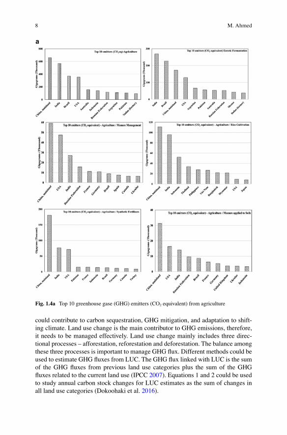
8

could contribute to carbon sequestration, GHG mitigation, and adaptation to shift-ing climate. Land use change is the main contributor to GHG emissions, therefore, it needs to be managed effectively. Land use change mainly includes three direc-tional processes – afforestation, reforestation and deforestation. The balance among these three processes is important to manage GHG flux. Different methods could be used to estimate GHG fluxes from LUC. The GHG flux linked with LUC is the sum of  the GHG fluxes  from previous  land  use  categories  plus  the  sum of  the GHG fluxes related to the current land use (IPCC 2007). Equations 1 and 2 could be used to study annual carbon stock changes for LUC estimates as the sum of changes in all land use categories (Dokoohaki et al. 2016).

Fig. 1.4a  Top 10 greenhouse gase (GHG) emitters (CO2 equivalent) from agriculture

M. Ahmed

9

D D DC C Cluc luco lucn= + (1)

D D D D DC C C C Cluc luc fl lu cl lu gl lu wl= + + +

(2)

where ΔC;  carbon  stock  change  (metric  tons CO2‐eq ha−1 year−1), luc; land use change, o; old land use, n; new land use, fl; forest land, cl; crop land, gl; grazing land and wl; wetlands.

Fig. 1.4b  Top 10 greenhouse gase (GHG) emitters (CO2 equivalent) from agriculture

1 Greenhouse Gas Emissions and Climate Variability: An Overview

10

The  annual  carbon  stock  exchange  for  a  particular  section  e.g.  management regime could be calculated by the following equation

C Cluciluc

i

n

= å D

(3)

where ΔCluc; carbon stock changes for a land use change and i denotes a specific division

Fig. 1.4c  Top 10 greenhouse gase (GHG) emitters (CO2 equivalent) from agriculture and land use change

M. Ahmed

11

Many  forest  and  agricultural  lands  have  live/dead  biomass  carbon  stocks (LDBCS) and soil organic carbon which acts as a good carbon store. The following equation (Dokoohaki et al. 2016) could be used to estimate the annual change in carbon stocks in dead wood due to land conversion.

D ¸C C C A Tdom n o on on= -( ) ×

(4)

where ΔCdom = annual change in carbon stocks in dead wood or litter (metric tons C year−1), Co = dead wood/litter stock, under the old land‐use category (metric tons C ha−1); Cn = dead wood/litter stock, under the new land‐use category (metric tons C ha−1), Aon = area undergoing conversion from old to new land‐use category (ha), Ton = time period of the transition from old to new land‐use category (year) (The default is 20 years for carbon stock increases and 1 year for carbon losses.)

Soil organic carbon stock  (SOCS)  is also  influenced by  land use change. The significant change in SOCS occurs due to conversion of land to crop land (Six et al. 2000). Aalde et al. (2006) proposed a method to estimate changes in SOCS from mineral soils.

D ¸C SOC SOC CO MW Dmineral f i 2= -( )éë ùû×

(5)

where ΔCmineral = annual  change  in  mineral  SOCS  (metric  tons  CO2‐eq year−1), SOCf = soil organic carbon stock at the end of year 5 (metric tons C), SOCi = soil organic carbon stock at the beginning of year 1 (metric tons C), CO2MW = ratio of molecular weight of CO2 to C (44/12 dimensionless) and D = time dependence of stock change factors (20 years).

Simialrly, SOCS from mineral soils could be calculated by using the following equation (Aalde et al. 2006)

SOCS SOC F F F Aref lu mg i= × × × ×

(6)

Fig. 1.4d  Top 10 greenhouse gase (GHG) emitters (CO2 equivalent) from agriculture and land use change

1 Greenhouse Gas Emissions and Climate Variability: An Overview

12

where SOCS = soil organic carbon stock at the beginning (SOCSi) and end of the 5 years (SOCSf) (metric tons C), SOCref = reference soil organic carbon stock (met-ric tons C ha−1), Flu = stock change factor for land use (dimensionless), Fmg = stock change factor for management (dimensionless), Fi = stock change factor for input (dimensionless) and A = area of land‐use change (ha).

Uncertainty analysis is an important technique to quantify the uncertainty of greenhouse gas (GHG) emissions from different sectors. It can help policy makers and farmers decide management options to minimize GHG emissions based upon an uncertainty range. If uncertainty for an estimate is low farmers can invest in that management practices as it has high probability of GHG emission reduction. A Monte Carlo approach  is a comprehensive,  sound method  that could be used for estimating the uncertainty. Greenhouse Gas Emissions and Climate Variability: An Overview covers the GHG emission status by different sectors and how it could be mitigated by using different practices in agriculture and land use sectors. This chap-ter reviews available methods for studying/quantifying GHG emission for accurate design of strategies to address the issue of climate variability.

1.2 Greenhouse Gas Emission and Climate Variability

Climate variability is one of the burning issues in all fields from social sciences to the  applied  sciences.  Climate  vulnerability  threatens  global  climatic  cycles  and world food production systems, thus affecting the lives of all people. Most of the world is exposed to the effects of climatic change due to extreme variability in tem-perature and rainfall. Risk reduction represents a major avenue for responding to existing  rise  in  temperature,  carbon  dioxide,  GHGs,  flood  and  drought  hazards. Global warming is the greatest environmental challenge of the twenty-first century as it results in increased average air temperature (Gnansounou et al. 2004). Wu et al. (2010) concluded that cities act as heat islands and since large areas of grassland and forest were converted to barren land resulted in greater climate variability. The guiding principle to reduce climate risks is to minimize GHG emission. In recent decades significant changes in the atmospheric temperature have been observed. The global mean annual temperature at the end of the twentieth century was almost 0.7 °C and it is likely to increase further by 1.8–6.4 °C by the end of this century (IPCC 2007). The warmest decade in the last 300 years was 1990–2000 with the increase of 0.5 °C in comparison to the baseline temperature of 1961–1990. A vari-ety of models ranging from simple models to complex earth system models were used to project future warming under different representative concentration path-ways (RCPs). The RCP includes RCP 2.6, RCP 4.5, RCP 6.0 and RCP 8.5 (The numbers refer to the rate of energy increase per unit area at the surface of the earth, in watts per square meter). RCP 2.6 is the normal scenario in which a guideline was established  to  limit global warming  to 2 °C (3.6 °F) above  the  level  that existed before industrial times. All other scenarios reflect severe warming due to increasing rates of GHG emission. The scenario RCP 8.5 reflects “business as usual” in which 

M. Ahmed

13

no policies are implemented to limit GHG emission. The projected increase in mean temperature and rise in sea level in comparison to baseline (1986–2005) are pre-sented in Table 1.1 (Harris et al. 2015). Climate variability resulted in a change in the intensity and frequency of rainfall which increased flooding and soil erosion.

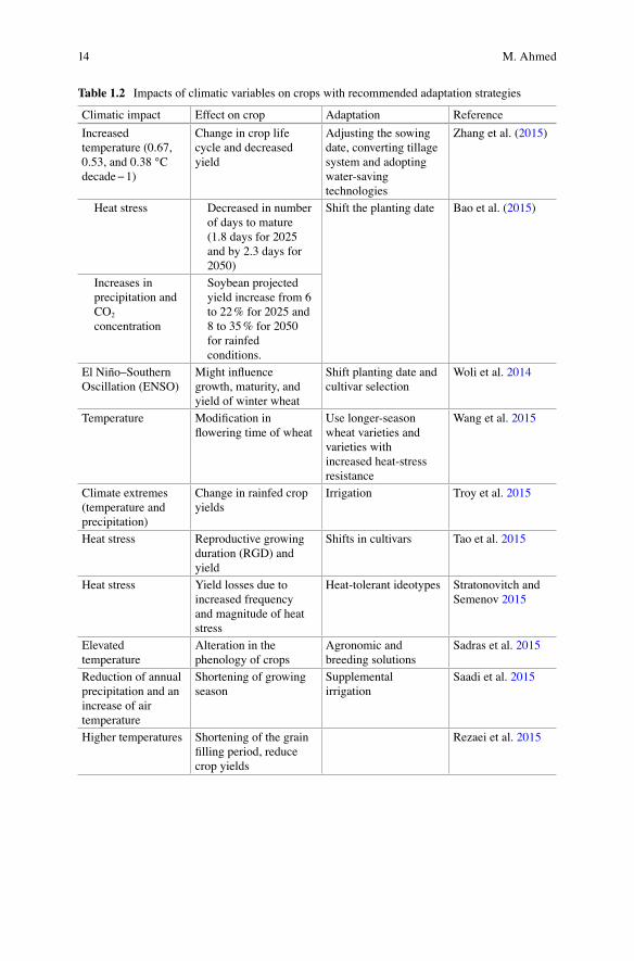
Crop phenology and productivity will be affected by warmer climates. Craufurd and Wheeler (2009) reported earlier flowering and maturity due to a rise in tempera-ture. Moreover,  increased  temperature  resulted  in  reproductive  failure  and  yield reductions in many crops. Lobell et al. (2011) reported a 1.7 % reduction in maize yield due to exposure of maize to degree days above 30 °C. Increased night tem-perature is another effect of GHG which could reduce crop yield. Serious effects have been reported for rice where an increase in night temperature from 27 °C to 32 °C caused 90 % yield reduction (Mohammed and Tarpley 2009). Climate vari-ability can also modify grain quality since high temperature during grain filling affects the protein content of wheat (Hurkman et al. 2009). Pittock (2003) con-cluded in their findings that the frequency of extreme events will  increase due to global warming. Plant processes like photosynthesis will be affected by high tem-perature which could lead to reduction in growth and yield (Calderini and Reynolds 2000; Talukder et al. 2014; 2013; Wang et al. 2011) (Table 1.2).

A panel of the National Research Council (United States) (2010) on advancing the science of climate change concluded that world mean temperature was 0.8 °C higher during the first decade of twenty-first century compared to first decade of twentieth century. Moreover, they reported that most of the warming was related to CO2 and other GHGs which can trap heat. The energy sector is the largest contribu-tor to climate change as it involves burning of fossil fuels (coal, oil, and natural gas). Similarly, the panel identified agriculture, forest clearing, and certain industrial activities as big contributors to climate change due to emission of GHGs. Kang and Banga (2013) found that climate change is a well-recognized man made global environmental challenge and that agriculture is significantly influenced by it. Food and Agriculture Organization (FAO) experts reported that each 1 °C rise in tempera-ture would cause annual wheat yield loss of about 6 million tons. However, when

Table 1.1  Changes in global mean surface temperature in °C and global mean sea level rise in m (bottom) for the two time periods shown, referenced to the baseline period 1986–2005 (The “likely range” gives confidence limits for a 5–95 % interval)

Climate variableRCP scenario

2046–2065 2081–2100

Mean Range Mean Range

Mean temperature change (°C) RCP2.6 1 0.4–1.6 1 0.3–1.7

RCP4.5 1.4 09–2.0 1.8 1.1–2.6

RCP6.0 1.3 0.8–1.8 2.2 1.4–3.1

RCP8.5 2 1.4–2.6 3.7 2.6–4.8

Mean Range Mean RangeMean Sea Level Rise (m) RCP2.6 0.24 0.17–0.32 0.4 0.26–0.55

RCP4.5 0.26 0.19–0.33 0.47 0.32–0.63

RCP6.0 0.25 0.18–0.32 0.48 0.33–0.63

RCP8.5 0.3 0.22–0.38 0.63 0.45–0.82

1 Greenhouse Gas Emissions and Climate Variability: An Overview

14

Table 1.2 Impacts of climatic variables on crops with recommended adaptation strategies

Climatic impact Effect on crop Adaptation Reference

Increased temperature (0.67, 0.53, and 0.38 °C decade − 1)

Change in crop life cycle and decreased yield

Adjusting the sowing date, converting tillage system and adopting water-saving technologies

Zhang et al. (2015)

Heat stress Decreased in number of days to mature (1.8 days for 2025 and by 2.3 days for 2050)

Shift the planting date Bao et al. (2015)

Increases in precipitation and CO2 concentration

Soybean projected yield increase from 6 to 22 % for 2025 and 8 to 35 % for 2050 for rainfed conditions.

El Niño–Southern Oscillation (ENSO)

Might influence growth, maturity, and yield of winter wheat

Shift planting date and cultivar selection

Woli et al. 2014

Temperature Modification in flowering time of wheat

Use longer-season wheat varieties and varieties with increased heat-stress resistance

Wang et al. 2015

Climate extremes (temperature and precipitation)

Change in rainfed crop yields

Irrigation Troy et al. 2015

Heat stress Reproductive growing duration (RGD) and yield

Shifts in cultivars Tao et al. 2015

Heat stress Yield losses due to increased frequency and magnitude of heat stress

Heat-tolerant ideotypes Stratonovitch and Semenov 2015

Elevated temperature

Alteration in the phenology of crops

Agronomic and breeding solutions

Sadras et al. 2015

Reduction of annual precipitation and an increase of air temperature

Shortening of growing season

Supplemental irrigation

Saadi et al. 2015

Higher temperatures Shortening of the grain filling period, reduce crop yields

Rezaei et al. 2015

M. Ahmed

15

losses of all other crops were taken into consideration it might cause loss of US$ 20 billion each year (Swaminathan and Kesavan 2012).  Climate  variability  can reduce crop duration, disturb source sink relationships, increase crop respiration, affect survival and distribution of pest populations, accelerate nutrient mineraliza-tion and decrease nutrient use efficiency. It can also lead to changes in the frequency and intensity of drought and floods (Sharma and Chauhan 2011). Overall agricul-tural production will be significantly affected by climate variability which will influence food security.

1.3 Greenhouse Gas Mitigation and Climate Change Adaptation

Climate change is one of the complex burning issues currently faced by the world. Greenhouse gases are trapping heat energy which results in global warming. It has been reported earlier that if GHGs are stopped completely, climate change will still affect future generations. Therefore, we need to show a high level of commitment to tackle the issue of climate change. Mitigation and adaptation are two approaches used to respond to climate change. Mitigation involves reducing and stabilizing the levels of GHGs while adaptation is adapting to climate change using different tech-niques. Mitigation is possible by finding ways by which we can increase sinks for GHGs. Mainly the sinks includes forests, soil and oceans, therefore it is necessary to manage  those  resources which  can  absorb GHGs. According  to Calvin  et  al. (2015) around 40 % of GHG emissions are from agriculture, forestry, and other land use (AFOLU). Their work further elaborated that implementation of climate policy is necessary to minimize GHG emissions. A multi-model comparison approach was used to study the future trajectory of AFOLU GHG emissions with and without mitigation. a similar approach about the role of land for the mitigation of AFOLU GHG emissions was earlier reported which includes the use of bioenergy crops (Calvin et al. 2013). The models used were Applied Dynamic Analysis of the Global Economy (ADAGE) (Ross 2009.); MIT Emissions Prediction and Policy Analysis (EPPA) (Paltsev et al. 2005); GCAM (Global Change Assessment Model) (Calvin et al. 2011) and TIAM-WORLD (Loulou 2008). The results indicated larger uncer-tainties in both present and future emissions with and without climate policy.

Bioenergy crops are the biggest potential source that could be used to minimize GHG emissions. Hudiburg et al. (2015) proposed perennial grasses as effective bio-energy crops on marginal lands. They evaluated the DayCent biogeochemical model in their studies and concluded that the model predicted yield and GHG fluxes with good accuracy. They found that with the replacement of traditional corn-soybean rotation with native prairie, switchgrass, and Miscanthus resulted in net GHG reduc-tions of 0.5, 1.0 and 2.0 Mg C ha−1 year−1 respectively. Since bioenergy crops have the potential to mitigate climate change impacts, they have been under consider-ation for the past decade. However, these bioenergy crops could only be grown on marginal lands as most of the world land is occupied by major food crops. Albanito

1 Greenhouse Gas Emissions and Climate Variability: An Overview

16

et al. (2016)  reported C4 grasses  (Miscanthus  and  switch-grass)  as  the  potential bioenergy crops with the highest climate mitigation potential. These crops would displace 58.1 Pg of fossil fuel C equivalent (Ceq oil) if the proposed land use change took place. Similarly, woody energy crops (poplar, willow and Eucalyptus species) could displace 0.9 Pg Ceq oil under proposed land use change. The best climate miti-gation option is the afforestation of suggested cropland which would sequester 5.8 Pg C in biomass in the 20-year-old forest and 2.7 Pg C in soil. Croplands could not accumulate carbon for more than a year therefore, in order to mitigate climate change, agricultural lands should either be converted to forest land or bioenergy production (Fig. 1.5). Food security will be a big challenge in the future as the world population will be 9–10 billion by 2050. Therefore, bioenergy crops could not come at the expense of food crops. Earlier researchers accepted the potential of biomass energy production but according to them it was not enough to replace just a few percent of current fossil fuel usage. Increasing biomass energy production beyond a certain level might imperil food security and worsen condition of climate change (Field et al. 2008). However, biomass proponents are recommending the use of grasslands and marginal crop lands as potential sites for bioenergy crops (Qin et al. 2015; Slade et al. 2014). Furthermore, Qin et al. (2015) suggested Miscanthus as the best potential crop to mitigate GHGs emissions on marginal lands compared to switchgrass. Biomass and ethanol yield were higher in Miscanthus. Coyle (2007) concluded that different crops, e.g. corn, sugarcane, rapeseed and soybean could be

Fig. 1.5  Carbon implications of converting cropland to forest or bioenergy crops for climate miti-gation: a global assessment (Source: Albanito et al. 2016)

M. Ahmed

17

used to produce biofuel. Energy potential from different feedstocks have been pre-sented in Table 1.3.

Chum et al. (2011) considered bioenergy as a good renewable source for energy. Bioenergy can easily replace fossil fuels and minimize GHG emissions (Dornburg and Faaij 2005; Dornburg et al. 2008; 2010). Implementation of all these techniques requires identification of terrestrial ecosystems which could contribute to climate mitigation. Many  countries  have  announced  different  targets  to  substitute  fossil fuels with biofuels (Ravindranath et al. 2008). Table 1.4 shows that C4 bioenergy crops have higher  cumulative  carbon mitigation potential  than SRCW. However, this mitigation potential changes across the continents as in Oceania, SRCW pro-duced  higher  C  savings  than  energy  crops. According  to Albanito  et  al.  (2016) cumulative carbon strength due to reforestation is highest in Asia, followed by Africa, North and Central America, South America, Oceania and Europe. However, on a per hectare basis C sequestration strength is higher in South America followed by North and Central America, Oceania, Asia, Africa and Europe. Among climatic regions, warm-dry climates could save 44.7 % of the C in forest followed by warm- moist (42.6 %), cool-dry (11.3 %) and cool-moist (1.4 %) regions (Table 1.5).

Biochar also has potential to mitigate climate change by sequestering carbon. Biochar use improved soil fertility, reduced fertilizer inputs, GHG emissions, and emissions from feedstock, enhanced soil microbial life and energy generation. Its use also increased crop yield. (Woolf et al. 2010) reported that biochar use could minimize GHG emissions by 12 %. The concept of sustainable use of biochar is presented in Fig. 1.6 as proposed by (Woolf et al. 2010). Photosynthesis is a carbon reduction processes  in which plants produce biomass by using atmospheric CO2. Residues from crops and forests were subjected to the process of pyrolysis which produced bio-oil, syngas, process heat and biochar (output). These outputs serve as a good source of energy which could minimize GHG emissions. Furthermore, bio-

Table 1.3 Energy potential from biofuel crops using current technologies and future cellulosic technologies

FTFM (Mt year−1)

GBC (GJ/ton)

GBE (EJ year−1)

NEBR (Output/Input)

NBE (EJ year−1) Refs

Corn kernel 696 8 5.8 1.25 1.2 Hill et al. 2006

Sugar cane 1324 2 2.8 8 2.4 IEA 2004

Cellulosic biomass

– 6 – 5.44 – Farrell et al. 2006

Soy oil 35 30 1 1.93 0.5 Worldwatch 2006

Palm oil 36 30 1.1 9 1 Worldwatch 2006

Rape oil 17 30 0.5 2.5 0.3 IEA 2004

Source: Field et al. (2008)Where FT Feedstock type, FM Feedstock mass, GBC Gross biofuel conversion (Useful biofuel energy per ton of crop for conversion into biofuel (1GJ = 109 J)), GBE Gross biofuel energy (Product of feedstock mass and gross biofuel conversion (1EJ = 1018 J)), NEBR Net energy balance ratio (Ratio of the energy captured in biomass fuel to the fossil energy input) and NBE Net biofuel energy (Energy yield above the fossil energy invested in growing, transporting and manufacturing, calculated as gross biofuel energy × (net energy balance ratio −1)/net energy balance ratio)

1 Greenhouse Gas Emissions and Climate Variability: An Overview

18

char could also be used to improve agricultural soils (Fig. 1.6). Roberts et al. (2009) suggested biochar (biomass pyrolysis) as a good source to mitigate climate change and minimize fossil fuel consumption. They used life cycle assessment (LCA) to estimate the impact of biochar on energy and climate change and concluded that biochar resulted in negative net GHG emissions. However, the economic viability of biochar production depends upon the cost of feedstocks. Similarly, a well-to-wheel (WTW) LCA model was developed  to assess  the environmental profile of  liquid fuels through pyrolysis (Kimball 2011). Bruckman et al. 2014 reported biochar as a potential geoengineering method to mitigate climate change and design adaptation strategies. Biochar as a soil amendment can sequester C and it is a useful option to mitigate climate change (Hudiburg et al. 2015). Biochar stability and decomposi-tion are the best criteria to evaluate its contribution to carbon (C) sequestration and climate change mitigation. (Macleod et al. 2015) reported that around 97 % of bio-char contributes directly to C sequestration in soil. Similarly, the biochar effect on soil organic matter (SOM) dynamics depends upon characteristics of biochar and 

Table 1.4  Land use change C mitigation potential

Land use CR TCM CMB CSSS ALD

C4 Bioenergy crops Asia 27.62 24.06 3.56 66.07

Africa 8.58 7.69 0.89 61.23

Europe 10.86 7.74 3.12 123.21

North America

10.49 8.89 1.6 74.34

South America

10.71 9.58 1.13 58.08

Oceania 0.19 0.16 0.03 1.98

Forest Asia 3.84 2.73 1.11 94.52

Africa 1.56 1.11 0.44 42.31

Europe 0.31 0.17 0.15 9.97

North America

1.47 0.96 0.5 24.67

South America

0.74 0.41 0.34 6.27

Oceania 0.51 0.39 0.12 8.7

Short Rotation Coppice Woody (SRCW) crops

Asia 0.48 0.2 0.28 10.49

Africa 0.0045 0.0019 0.0026 0.35

Europe 0.92 0.52 0.41 12.54

North America

0.18 0.1 0.07 2.38

South America

0.03 0.03 0.01 0.46

Oceania 0.01 0.01 0 0.13

Source: Albanito et al. (2016)Where CR Continental region, TCM Total C mitigated, CMB C mitigated from biomass use/incre-ment (Pg C forest and Pg Ceq oil for bioenergy crops), CSSS C stock sequestered in soil (Pg C) and ALD; Agricultural land displaced (Mha)

M. Ahmed

19

Table 1.5  Land use change C mitigation potential across global climatic regions

Land use CR TCM CMB CSSS ALD

C4 Bioenergy crops CD 1.69 0.84 0.85 32.47

CM 18.06 13.94 4.12 176.74

WD 0.1 0.08 0.02 2.2

WM 48.59 43.26 5.33 273.49

Forest CD 0.95 0.59 0.36 47.38

CM 0.12 0.04 0.08 2.67

WD 3.77 2.84 0.93 90.96

WM 3.6 2.3 1.3 45.44

Short Rotation Coppice Woody (SRCW) crops CD 0.42 0.06 0.36 13.53

CM 1.05 0.68 0.38 10.37

WD 0.01 0.01 0.01 0.85

WM 0.14 0.12 0.02 1.6

Source: Albanito et al. (2016)Where CR Climate region, TCM Total C mitigated, CMB C mitigated from biomass use/increment (Pg C forest and Pg Ceq oil for bioenergy crops), CSSS C stock sequestered in soil (Pg C), ALD Agricultural land displaced (Mha), CD Cool-Dry, CM Cool-Wet, WD Warm-Dry and WM Warm moist

Fig. 1.6 Sustainable biochar concept (Source: Woolf et al. 2010)

1 Greenhouse Gas Emissions and Climate Variability: An Overview