quality assurance project plan cfd modeling for ut/tceq low...
TRANSCRIPT
Page 1
February 2011, Rev. 4
Air Quality Research Program Project 10-022
Quality Assurance Project Plan
CFD Modeling for UT/TCEQ Low BTU & Low Flow Rate Flare Tests
Prepared by:
Daniel Chen, PI
Helen Lou, Co-PI Kuyen Li, Co-PI
Dan F. Smith Department of Chemical Engineering, Lamar University
Christopher Martin, Co-PI Department of Chemistry & Biochemistry, Lamar University
X. Chang Li, Co-PI Department of Mechanical Engineering, Lamar University
Page 2
Page 3
1.2 Distribution List Jim MacKay TCEQ Project Liaison Air Quality Division Texas Commission on Environmental Quality Austin, Texas Mr. Vincent M. Torres Project Manager Air Quality Research Program The University of Texas at Austin, Austin, Texas Dr. Daniel H. Chen Principal Investigator Lamar University, Beaumont, Texas 1.3 General Requirements This project is a secondary data project. A secondary data project involves the gathering and /or use of existing environmental data for purposes other than those for which they were originally collected. This document is based on EPA’s National Risk Management Research Laboratory (NRMRL) QAPP for secondary data project and satisfies a Category III level of QA.
Page 4
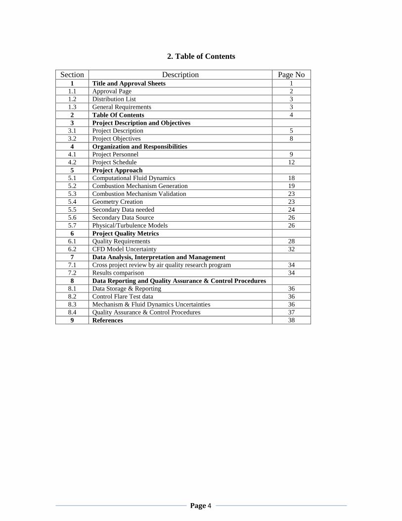
2. Table of Contents
Section Description Page No
1 Title and Approval Sheets 1 1.1 Approval Page 2 1.2 Distribution List 3 1.3 General Requirements 3 2 Table Of Contents 4 3 Project Description and Objectives
3.1 Project Description 5 3.2 Project Objectives 8 4 Organization and Responsibilities
4.1 Project Personnel 9 4.2 Project Schedule 12 5 Project Approach
5.1 Computational Fluid Dynamics 18 5.2 Combustion Mechanism Generation 19 5.3 Combustion Mechanism Validation 23 5.4 Geometry Creation 23 5.5 Secondary Data needed 24 5.6 Secondary Data Source 26 5.7 Physical/Turbulence Models 26 6 Project Quality Metrics
6.1 Quality Requirements 28 6.2 CFD Model Uncertainty 32 7 Data Analysis, Interpretation and Management
7.1 Cross project review by air quality research program 34 7.2 Results comparison 34 8 Data Reporting and Quality Assurance & Control Procedures
8.1 Data Storage & Reporting 36 8.2 Control Flare Test data 36 8.3 Mechanism & Fluid Dynamics Uncertainties 36 8.4 Quality Assurance & Control Procedures 37 9 References 38

Page 5
Quality Assurance Project Plan
3. PROJECT DESCRIPTION AND OBJECTIVES
3.1 Project Description
Current methodologies for calculating speciated and total VOC emissions from
flaring activities generally apply a simple mass reduction to the VOC species sent to the
flare1. In most cases 98% is used as the destruction and removal efficiency (DRE) for the
flare without any intermediate VOC species generated or emitted by the combustion
process. Basic combustion chemistry demonstrates that many intermediate VOC species
are formed by the combustion process. While it is assumed that a flare operating under
its designed conditions and in compliance with 40 CFR 60.18 may achieve 98% DRE or
higher a flare operating outside of these parameters may have a DRE lower than 98%2.
Other factors that may affect DRE and the combustion efficiency (CE) include
environmental factors such as cross wind, ambient temperature, and humidity3,4,5
In this project, computational fluid dynamics (CFD) methods based on CHEMKIN –
CFD and FLUENT are used to model low-Btu, low-flow rate propylene/TNG/nitrogen
flare tests conducted during September, 2010 in the John Zink test facility in Tulsa,
Oklahoma6. In these flare performance tests, plume measurements using both remote
sensing and direct extraction were carried out to determine flare efficiencies and
concentration/location of regulated and photo chemically important pollution species for
air-assist and steam-assist flares. Various combinations of fuel BTU and flow rates were
performed under open-air conditions. This proposed project will primarily use CFD
modeling as a predicting tool for the Tulsa flare performance tests. However, if the test
data is available by May 31, 2011, the CFD modeling will be further compared with the
flare performance data, i.e., flare efficiencies, and other measurement data (e.g., species

Page 6
concentrations) reported in the TCEQ Comprehensive Flare Study Project. If the
difference between the model value and the test data is within the combined measurement
and prediction uncertainty limit (e.g., ±39% for CE & ±30%% for CO, and a factor of 3
for minor species such as formaldehyde, details see Sec. 7.2), the model value and the
test data will be considered as in good agreement. This modeling tool has the potential to
help TCEQ’s on-going evaluation on flare emissions and to serve as a basis for a future
SIP revision7.
Lamar University will model the data collected from the TCEQ Comprehensive Flare
Study Project (PGA No. 582-8-862-45-FY09-04)6 using computational fluid dynamics
(CFD) programs. The modeling programs used by Lamar University shall be CHEMKIN
and FLUENT.
GRI-Mech 3.0 is an optimized mechanism designed to model natural gas (C1)
combustion, including NO formation and reburn chemistry while USC is an Optimized
Reaction Model of C1-C3 Combustion but lacks chemistry needed to define NO
formation for flaring in air. So the inclusion of NO formation chemistry from the GRI
mechanism will make the USC mechanism suitable for modeling Tulsa test flares (that
burn fuel C1 & C3 and measure NO emission). Ideally the combined and individually
optimized components can be optimized again as a whole. From an engineering point of
view, since that bulk of the mechanism (USC) has been optimized, we only need to
demonstrate this mechanism is applicable and is validated. Indeed, this mechanism has
been tested against methane, ethylene, and propylene experimental data like laminar
flame speed, adiabatic flame temperature, and ignition delay8. We will also add a couple
of NOx species that are important to atmospheric chemistry (NO2 and HONO) to the
existing mechanism and a comparison with lab data will be carried out to evaluate this
new mechanism.9

Page 7
Lamar University will acquire the operating and design data of the flare tests
conducted at the John Zink facility in Tulsa, OK from the University of Texas. These
input data should include the geometry of the steam-assist and air-assist flares used in the
tests (AutoCad sketch with data preferred), meteorological data (cross-wind
speed/direction, humidity, temperature), and the operating data (aeration, steaming, exit
velocity, waste gas/pilot fuel species) available from the data acquisition system. If
Lamar University acquires the flare test data conducted at the John Zink facility in Tulsa,
OK from the University of Texas by May 31, 2011, the test data will be compared with
the model results to see if they are in good agreement, i.e., within the combined
uncertainty limits. The flare test data include performance data: Combustion Efficiency
(CE)/ Destruction & Removal Efficiencies (DRE) and other measured data:
concentration/location/path of monitored emission species (VOC, CO/CO2, and NOx)
and plume temperature/ location/path. Regulated/monitored flare emissions include O2,
NO, NO2, CO, CO2, CH4, C2H2 (Acetylene), C2H4 (Ethylene), C3H6 (Propylene),
CH2O (Formaldehyde), C2H4O (Acetaldehyde), and C3H6O (Acetone) will also be
predicted10.
Combustion efficiency is defined as the percentage of flare emissions that are completely
oxidized to CO2. It can be written mathematically as:
100SootTHCCOCO
CO CE%2
2 ×+++
= (4.1)
Where:
CO2 - parts per million by volume of carbon dioxide
CO - parts per million by volume of carbon monoxide exiting from the flare
THC - parts per million by volume of total hydrocarbon exiting from the flare
Soot - parts per million by volume of soot as carbon
Page 8
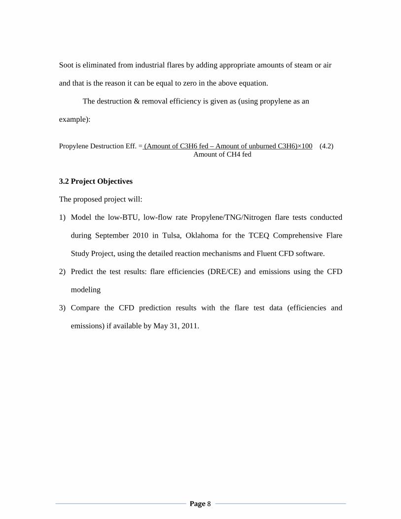
Soot is eliminated from industrial flares by adding appropriate amounts of steam or air
and that is the reason it can be equal to zero in the above equation.
The destruction & removal efficiency is given as (using propylene as an
example):
Propylene Destruction Eff. = (Amount of C3H6 fed – Amount of unburned C3H6)×100 (4.2)
Amount of CH4 fed
3.2 Project Objectives
The proposed project will:
1) Model the low-BTU, low-flow rate Propylene/TNG/Nitrogen flare tests conducted
during September 2010 in Tulsa, Oklahoma for the TCEQ Comprehensive Flare
Study Project, using the detailed reaction mechanisms and Fluent CFD software.
2) Predict the test results: flare efficiencies (DRE/CE) and emissions using the CFD
modeling
3) Compare the CFD prediction results with the flare test data (efficiencies and
emissions) if available by May 31, 2011.
Page 9
4. ORGANIZATION AND RESPONSIBILITIES
4.1 Project personnel
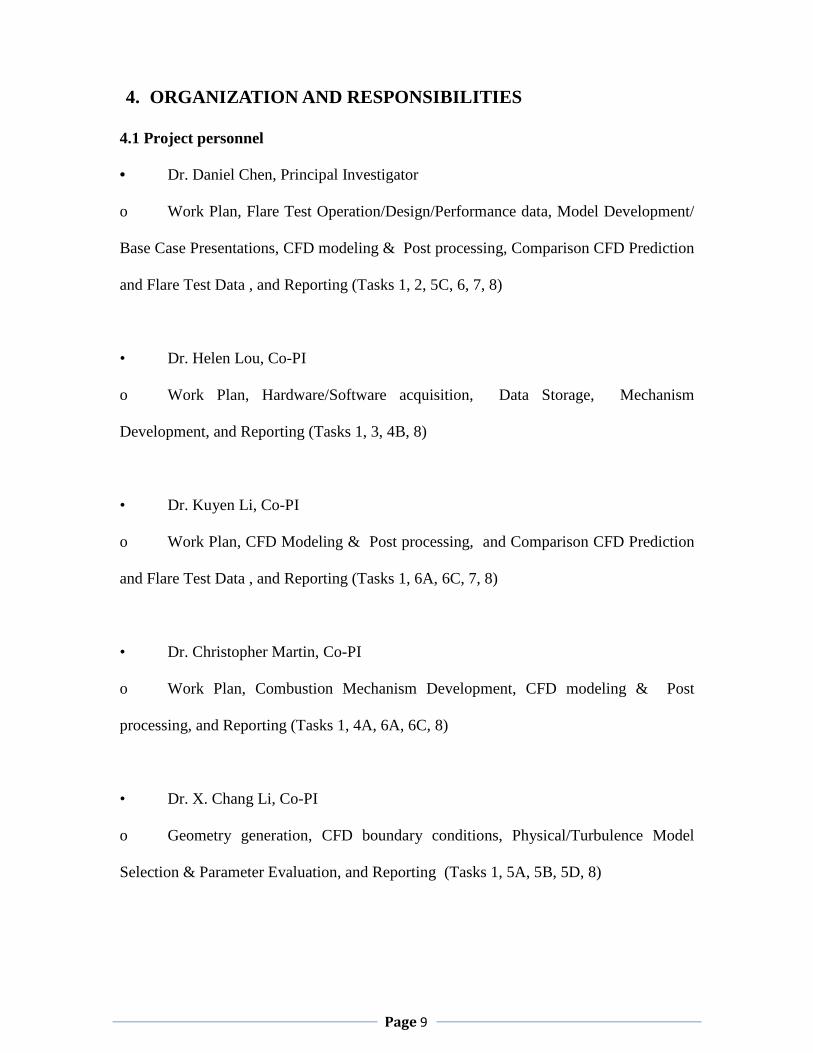
• Dr. Daniel Chen, Principal Investigator
o Work Plan, Flare Test Operation/Design/Performance data, Model Development/
Base Case Presentations, CFD modeling & Post processing, Comparison CFD Prediction
and Flare Test Data , and Reporting (Tasks 1, 2, 5C, 6, 7, 8)
• Dr. Helen Lou, Co-PI
o Work Plan, Hardware/Software acquisition, Data Storage, Mechanism
Development, and Reporting (Tasks 1, 3, 4B, 8)
• Dr. Kuyen Li, Co-PI
o Work Plan, CFD Modeling & Post processing, and Comparison CFD Prediction
and Flare Test Data , and Reporting (Tasks 1, 6A, 6C, 7, 8)
• Dr. Christopher Martin, Co-PI
o Work Plan, Combustion Mechanism Development, CFD modeling & Post
processing, and Reporting (Tasks 1, 4A, 6A, 6C, 8)
• Dr. X. Chang Li, Co-PI
o Geometry generation, CFD boundary conditions, Physical/Turbulence Model
Selection & Parameter Evaluation, and Reporting (Tasks 1, 5A, 5B, 5D, 8)
Page 10
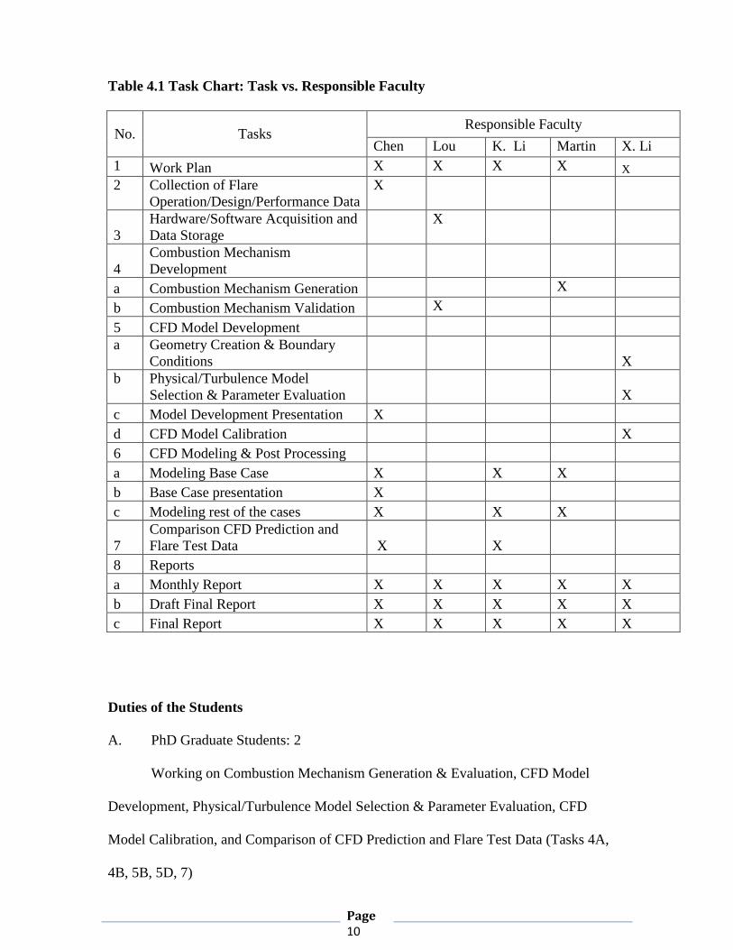
Table 4.1 Task Chart: Task vs. Responsible Faculty
No. Tasks Responsible Faculty
Chen Lou K. Li Martin X. Li 1 Work Plan X X X X X 2 Collection of Flare
Operation/Design/Performance Data X
3 Hardware/Software Acquisition and Data Storage
X
4 Combustion Mechanism Development
a Combustion Mechanism Generation X b Combustion Mechanism Validation X 5 CFD Model Development a Geometry Creation & Boundary
Conditions X b Physical/Turbulence Model
Selection & Parameter Evaluation X c Model Development Presentation X d CFD Model Calibration X 6 CFD Modeling & Post Processing a Modeling Base Case X X X b Base Case presentation X c Modeling rest of the cases X X X
7 Comparison CFD Prediction and Flare Test Data X X
8 Reports a Monthly Report X X X X X b Draft Final Report X X X X X c Final Report X X X X X
Duties of the Students
A. PhD Graduate Students: 2
Working on Combustion Mechanism Generation & Evaluation, CFD Model
Development, Physical/Turbulence Model Selection & Parameter Evaluation, CFD
Model Calibration, and Comparison of CFD Prediction and Flare Test Data (Tasks 4A,
4B, 5B, 5D, 7)
Page 11
B. MS Research Assistants: 3
Working on Geometry Generation, Input Data File Preparation, CFD Modeling &
Post Processing, Comparison of CFD Prediction and Flare Test Data, and Data Storage.
(Tasks 2, 3, 5A, 6A, 6C, 7)
AQRP - Project Manager
Vincent M. Torres, MSE, PE, MAC
Air Quality Research Program
The University of Texas at Austin
10100 Burnet Road, Bldg. 133 (MC R7100)
Austin, TX 78751
TCEQ - Project Liaison
Air Quality Division/Air Modeling and Data Analysis Section
Texas Commission on Environmental Quality
Mail Code 164, P.O.Box 13087
12118 Park 35 Circle, Bldg. E
Austin, Texas 78711-3087
Page 12
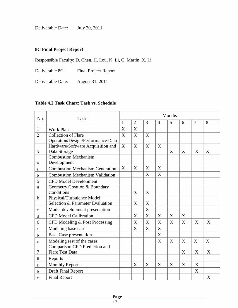
4.2 Project Schedule
The tasks are outlined below with corresponding deliverable date. The schedule is also
summarized in Table 4.1 & Table 4.2 as a matrix.
Task 1: Work Plan
Lamar University will submit a work plan with a work statement, QAPP, and budget.
The organization and task responsibilities are given below and in Section 5.
Responsible Faculty: D. Chen, H. Lou, K. Li, C. Martin, X. Li
Deliverable 1: Work Plan
Deliverable Date: February 9, 2011
Task 2: Flare Test Operation/Design/Performance Data
Lamar University will acquire the operating and design data of the flare tests conducted
at the John Zink facility in Tulsa, OK from the University of Texas. These data should
include the geometry of the steam-assist and air-assist flares used in the test (AutoCad
sketch with data preferred), meteorological data (cross-wind speed/direction, humidity,
temperature), and the operating data (aeration, steaming, exit velocity, waste gas/pilot
fuel species) available from the data acquisition system. If Lamar University acquires the
test data conducted at the John Zink facility in Tulsa, OK from the University of Texas
by May 31, 2011, the test data will be compared with the model results. The flare
Design/test Operation data from UT will be organized into input files for Fluent
simulations such as geometry generation, fuel/steam/flow/crosswind specifications. Flare
test data, if received by May 31, 2011, will be used to carry out Task 7. We need a base
case of air-assist flare and another base case for steam-assist flare. For each base case, we
need to run 2 more air (or steam) flow rates. We also run 2 more LHV cases for each
flare. So the total number of cases will be 2 (base cases) + 2 (additional air flow rates) +
Page 13
2 (additional steam flow rates) + 2 (LHVs in air-assist flare) + 2 (LHVs in steam-assist
flare) =10 cases.
Responsible Faculty: D. Chen
Deliverable 2: Included in Monthly Reports
Deliverable Date: March 31, 2011.
Task 3: Hardware/Software Acquisition and Data Storage
Responsible Faculty: H. Lou
Deliverable 3: Included in Monthly and Final Reports
Deliverable Date: Same as the due date for Task 8
Task 4: Combustion Mechanism Development
The details of combustion mechanism development are given in Sections 6.2 - 6.3. The
role of individual faculty is given below and Section 5.
4A Combustion Mechanism Generation
Responsible Faculty: C. Martini (Combustion Mechanism Generation)
Deliverable 4A: Included in Monthly Reports
Deliverable Date: The existing 50 species mechanism is fully functional. The next
version mechanism (USC + GRI 3.0) with additional NOx species will be delivered by
April 30, 2011.
4B Combustion Mechanism Validation
Responsible Faculty: H. Lou
Deliverable 4B: Included in Monthly Reports

Page 14
Deliverable Date: The data pertinent to the validation (or performance evaluation) of
the new mechanism (USC + GRI 3.0) with additional NOx species will be delivered in
April 30, 2011.
Task 5: CFD Model Development
The details of the CFD model development are given in Sections 6.4 - 6.7.
5A. Geometry Creation & Boundary Conditions
The details of the Geometry Creation & Boundary Conditions are given in Sections 6.4.
Responsible Faculty: X. Li
Deliverable 5A: Included in Monthly Reports
Deliverable Date: March 31, 2011
5B Physical/Turbulence Model Selection & Parameter Evaluation
The details of the Physical/Turbulence Model Selection & Parameter Evaluation are
given in Sections 6.7.
Responsible Faculty: X. Li
Deliverable 5B: Included in Monthly Reports
Deliverable Date: March 31, 2011
5C Model Development Presentation
The PI will provide a presentation to the AQRP Project Manager and the staff to review
the model development (Tasks 5A & 5B).
Responsible Faculty: D. Chen
Deliverable 5C: Model Development Presentation
Deliverable Date: March 31, 2011
Page 15
5D CFD Model Calibration
The selection of physical/turbulence models and parameters will be checked against
literature flare test data11,12,13 and will be varied if necessary to validate the CFD
modeling used in this project. The chosen physical/turbulence models, model parameters,
and simulation results will be delivered at the conclusion of this subtask.
Responsible Faculty: X. Li
Deliverable 5D: Included in Monthly Reports
Deliverable Date: June 30, 2011
Task 6: CFD Modeling & Post Processing
6A Modeling Base Case
Implement developed CFD modeling framework to run the selected Base Case.
Responsible Faculty: K. Li (CE & DRE), D. Chen (NOx Species) & C. Martin (VOC
Species)
Deliverable 6A: Included in Monthly and Final Reports
Deliverable Date: April 30, 2011
6B Base Case Presentation
The PI will present the results of the base case modeling (Task 6A) to the AQRP manager
and staff.
Responsible Faculty: D. Chen
Deliverable 6B: Base Case Presentation
Deliverable Date: April 30, 2011
Page 16
6C Modeling Rest of the Cases
Implement developed CFD modeling framework to run the 10 chosen Tulsa, OK Flare
test cases. The post-processing of CFD will predict flare efficiencies and the extent of
flare emissions.
Responsible Faculty: K. Li (CE & DRE), D. Chen (NOx Species) & C. Martin (VOC
Species)
Deliverable 6C: Included in Monthly and Final Reports
Deliverable Date: Same as the due date for Task 8.
Task 7: Comparison CFD Prediction and Flare Test Data
Comparison will be carried out if the data is provided by UT by May 31, 2011. The CFD
model will be validated using literature data.
Responsible Faculty: D. Chen (Species), K. Li (CE & DRE)
Deliverable 7: Included in Monthly and Final Reports
Deliverable Date: August 31, 2011
Task 8: Reports
8A Monthly Project Report
Responsible Faculty: D. Chen, H. Lou, K. Li, C. Martin, X. Li
Deliverable 8A: Monthly Project Report
Deliverable Date: 8th day of the month after the issue of the work order
8B: Draft Final Project Report
Responsible Faculty: D. Chen, H. Lou, K. Li, C. Martin, X. Li
Deliverable 8B: Draft Final Project Report
Page 17
Deliverable Date: July 20, 2011
8C Final Project Report
Responsible Faculty: D. Chen, H. Lou, K. Li, C. Martin, X. Li
Deliverable 8C: Final Project Report
Deliverable Date: August 31, 2011
Table 4.2 Task Chart: Task vs. Schedule
No. Tasks Months
1 2 3 4 5 6 7 8 1 Work Plan X X 2 Collection of Flare
Operation/Design/Performance Data X X X
3 Hardware/Software Acquisition and Data Storage
X X X X X X X X
4 Combustion Mechanism Development
a Combustion Mechanism Generation X X X X b Combustion Mechanism Validation X X 5 CFD Model Development a Geometry Creation & Boundary
Conditions X X b Physical/Turbulence Model
Selection & Parameter Evaluation X X c Model development presentation X d CFD Model Calibration X X X X X 6 CFD Modeling & Post Processing X X X X X X X a Modeling base case X X X b Base Case presentation X c Modeling rest of the cases X X X X X
7 Comparison CFD Prediction and Flare Test Data X X X
8 Reports a Monthly Report X X X X X X b Draft Final Report X c Final Report X
Page 18
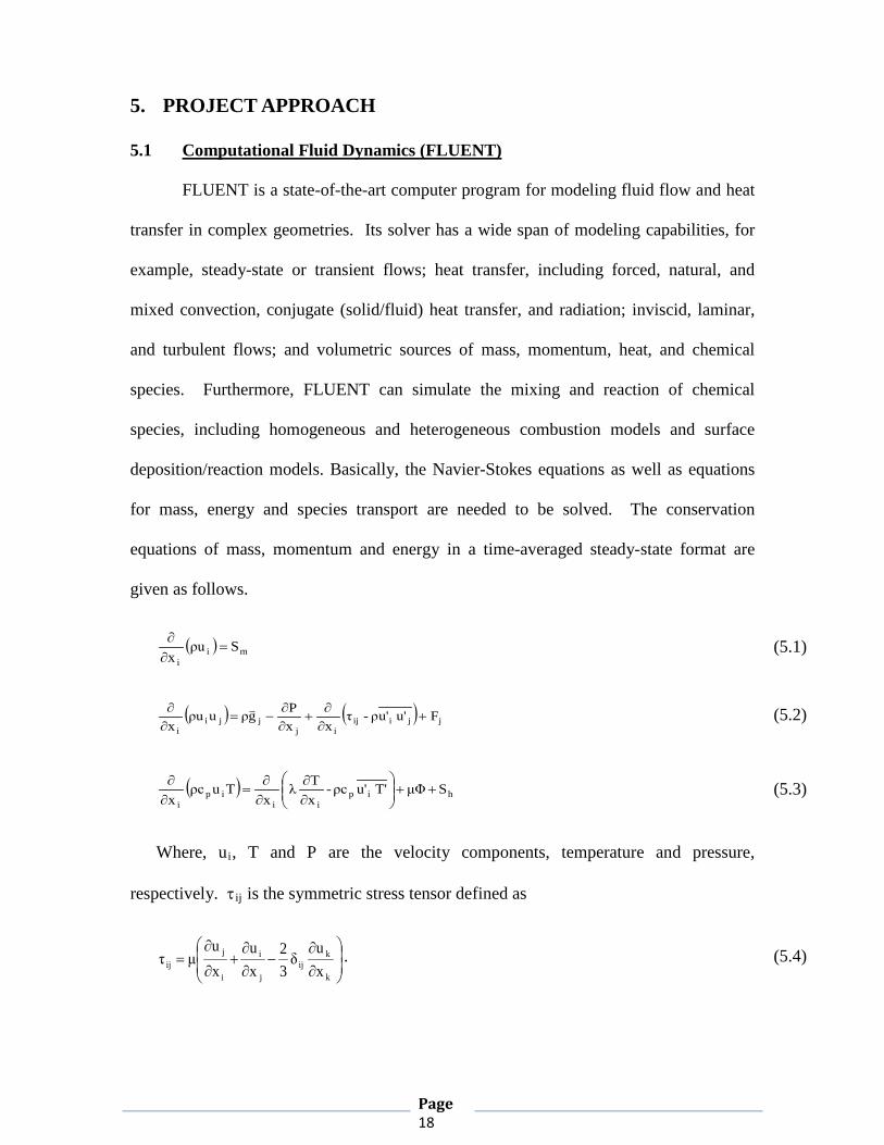
5. PROJECT APPROACH
5.1 Computational Fluid Dynamics (FLUENT)
FLUENT is a state-of-the-art computer program for modeling fluid flow and heat
transfer in complex geometries. Its solver has a wide span of modeling capabilities, for
example, steady-state or transient flows; heat transfer, including forced, natural, and
mixed convection, conjugate (solid/fluid) heat transfer, and radiation; inviscid, laminar,
and turbulent flows; and volumetric sources of mass, momentum, heat, and chemical
species. Furthermore, FLUENT can simulate the mixing and reaction of chemical
species, including homogeneous and heterogeneous combustion models and surface
deposition/reaction models. Basically, the Navier-Stokes equations as well as equations
for mass, energy and species transport are needed to be solved. The conservation
equations of mass, momentum and energy in a time-averaged steady-state format are
given as follows.
( ) mii
Sρux
=∂∂ (5.1)
( ) ( ) jjiijij
jjii
Fu'u'ρ-τxx
Pgρuρux
+∂∂
+∂∂
−=∂∂ (5.2)
( ) hipii
ipi
SμΦT'u'ρc-xTλ
xTuρc
x++
∂∂
∂∂
=∂∂ (5.3)
Where, ui, T and P are the velocity components, temperature and pressure,
respectively. τij is the symmetric stress tensor defined as
∂∂
−∂∂
+∂
∂=
k
kij
j
i
i
jij x
uδ
32
xu
xu
μτ . (5.4)
Page 19
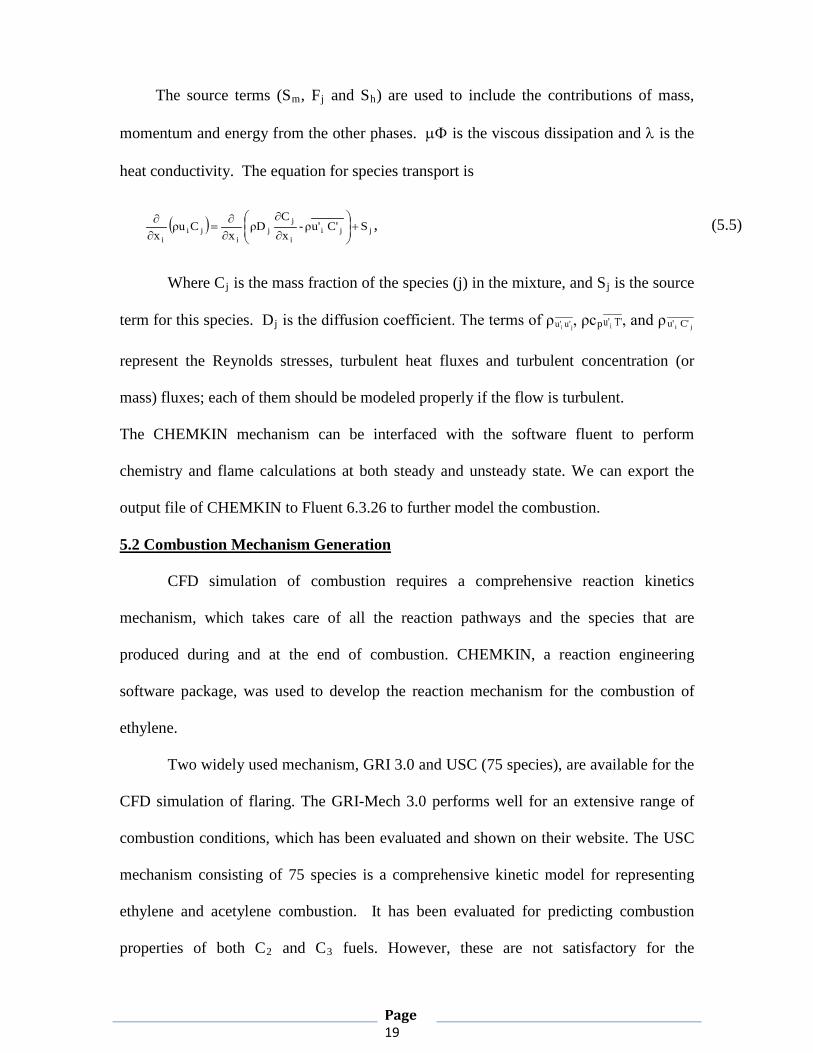
The source terms (Sm, Fj and Sh) are used to include the contributions of mass,
momentum and energy from the other phases. µΦ is the viscous dissipation and λ is the
heat conductivity. The equation for species transport is
( ) jjii
jj
iji
iSC'u'ρ-
xC
ρDx
Cρux
+
∂
∂
∂∂
=∂∂ , (5.5)
Where Cj is the mass fraction of the species (j) in the mixture, and Sj is the source
term for this species. Dj is the diffusion coefficient. The terms of ρji u'u' , ρcp T'u'i , and ρ ji C'u'
represent the Reynolds stresses, turbulent heat fluxes and turbulent concentration (or
mass) fluxes; each of them should be modeled properly if the flow is turbulent.
The CHEMKIN mechanism can be interfaced with the software fluent to perform
chemistry and flame calculations at both steady and unsteady state. We can export the
output file of CHEMKIN to Fluent 6.3.26 to further model the combustion.
5.2 Combustion Mechanism Generation
CFD simulation of combustion requires a comprehensive reaction kinetics
mechanism, which takes care of all the reaction pathways and the species that are
produced during and at the end of combustion. CHEMKIN, a reaction engineering
software package, was used to develop the reaction mechanism for the combustion of
ethylene.
Two widely used mechanism, GRI 3.0 and USC (75 species), are available for the
CFD simulation of flaring. The GRI-Mech 3.0 performs well for an extensive range of
combustion conditions, which has been evaluated and shown on their website. The USC
mechanism consisting of 75 species is a comprehensive kinetic model for representing
ethylene and acetylene combustion. It has been evaluated for predicting combustion
properties of both C2 and C3 fuels. However, these are not satisfactory for the
Page 20
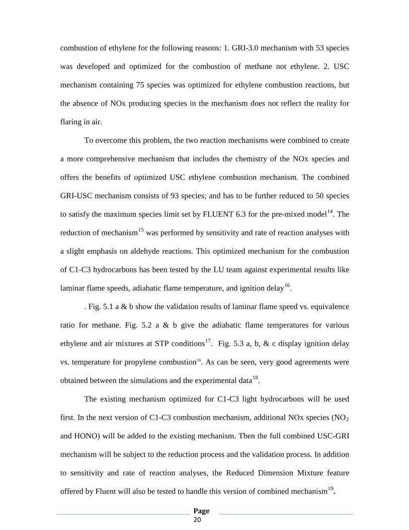
combustion of ethylene for the following reasons: 1. GRI-3.0 mechanism with 53 species
was developed and optimized for the combustion of methane not ethylene. 2. USC
mechanism containing 75 species was optimized for ethylene combustion reactions, but
the absence of NOx producing species in the mechanism does not reflect the reality for
flaring in air.
To overcome this problem, the two reaction mechanisms were combined to create
a more comprehensive mechanism that includes the chemistry of the NOx species and
offers the benefits of optimized USC ethylene combustion mechanism. The combined
GRI-USC mechanism consists of 93 species; and has to be further reduced to 50 species
to satisfy the maximum species limit set by FLUENT 6.3 for the pre-mixed model14. The
reduction of mechanism15 was performed by sensitivity and rate of reaction analyses with
a slight emphasis on aldehyde reactions. This optimized mechanism for the combustion
of C1-C3 hydrocarbons has been tested by the LU team against experimental results like
laminar flame speeds, adiabatic flame temperature, and ignition delay16.
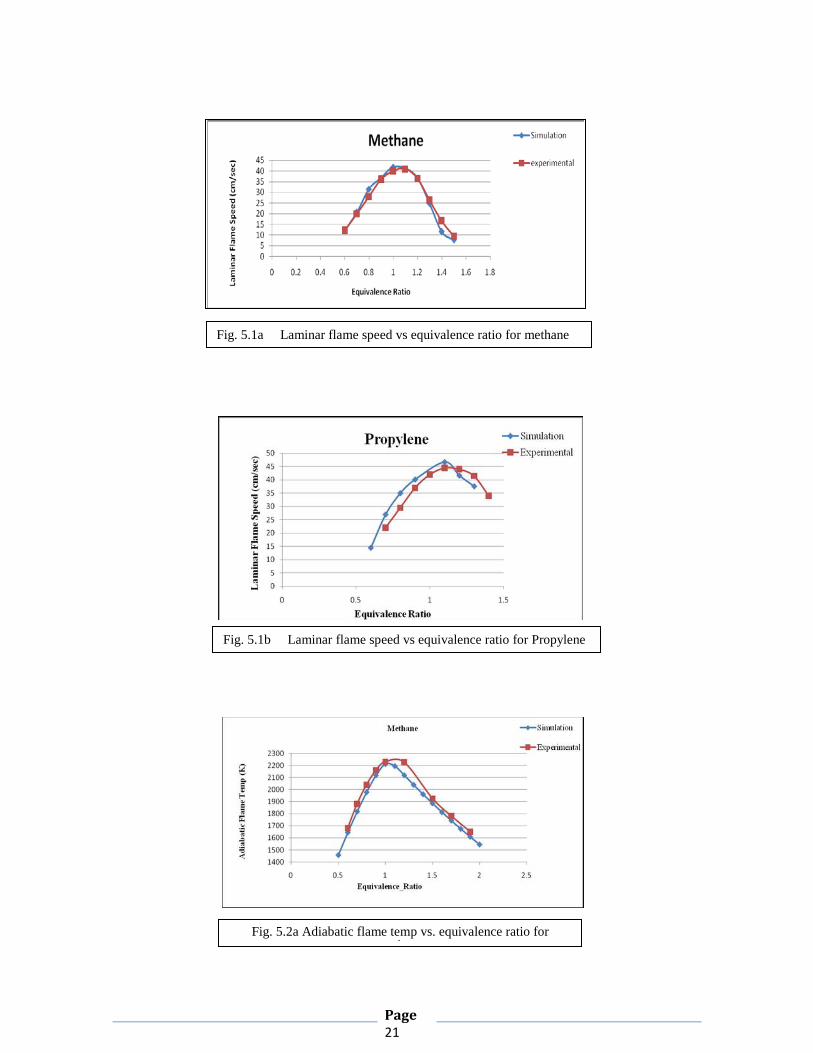
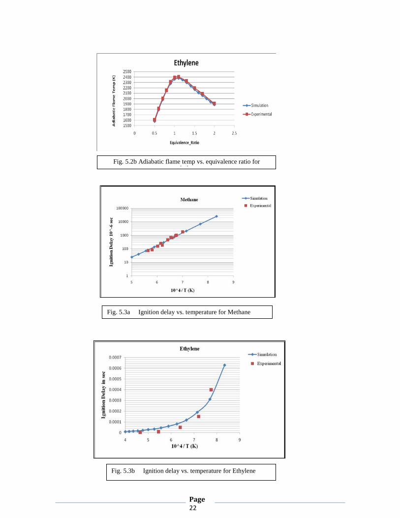
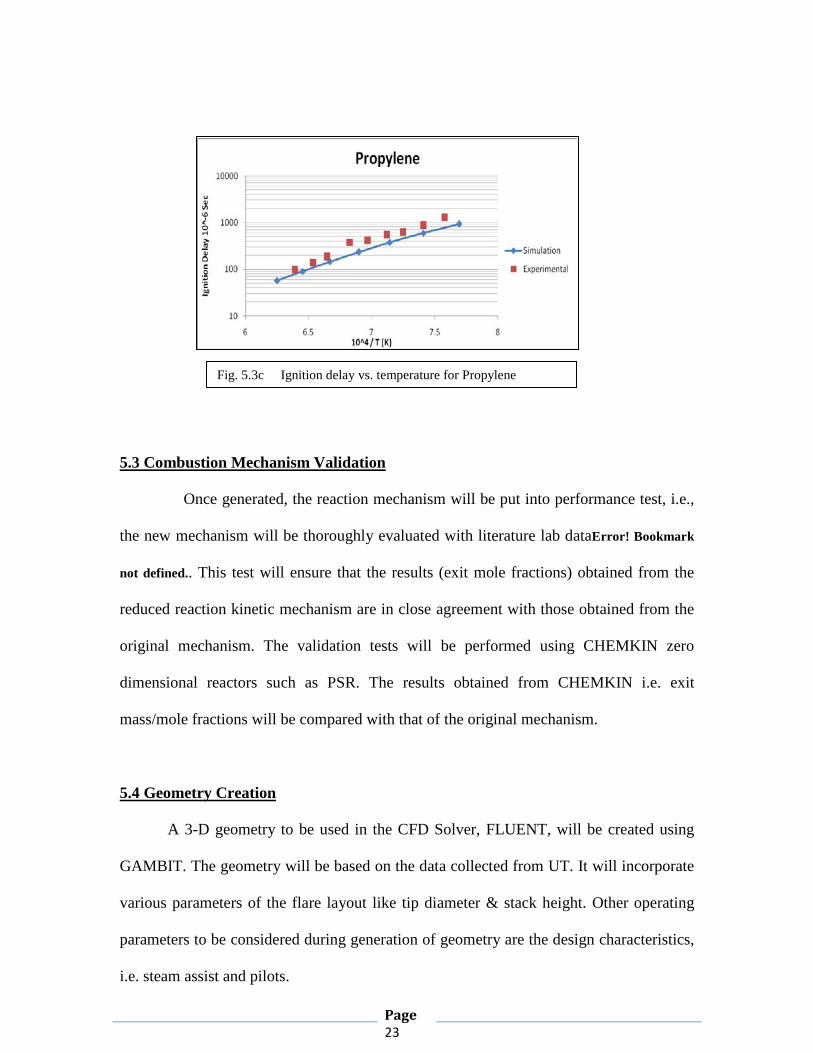
. Fig. 5.1 a & b show the validation results of laminar flame speed vs. equivalence
ratio for methane. Fig. 5.2 a & b give the adiabatic flame temperatures for various
ethylene and air mixtures at STP conditions17. Fig. 5.3 a, b, & c display ignition delay
vs. temperature for propylene combustion16. As can be seen, very good agreements were
obtained between the simulations and the experimental data18.
The existing mechanism optimized for C1-C3 light hydrocarbons will be used
first. In the next version of C1-C3 combustion mechanism, additional NOx species (NO2
and HONO) will be added to the existing mechanism. Then the full combined USC-GRI
mechanism will be subject to the reduction process and the validation process. In addition
to sensitivity and rate of reaction analyses, the Reduced Dimension Mixture feature
offered by Fluent will also be tested to handle this version of combined mechanism19.
Page 21
Fig. 5.2a Adiabatic flame temp vs. equivalence ratio for h
Fig. 5.1b Laminar flame speed vs equivalence ratio for Propylene
Fig. 5.1a Laminar flame speed vs equivalence ratio for methane
Page 22
Fig. 5.2b Adiabatic flame temp vs. equivalence ratio for th l
Fig. 5.3b Ignition delay vs. temperature for Ethylene
Fig. 5.3a Ignition delay vs. temperature for Methane
Page 23
5.3 Combustion Mechanism Validation
Once generated, the reaction mechanism will be put into performance test, i.e.,
the new mechanism will be thoroughly evaluated with literature lab dataError! Bookmark
not defined.. This test will ensure that the results (exit mole fractions) obtained from the
reduced reaction kinetic mechanism are in close agreement with those obtained from the
original mechanism. The validation tests will be performed using CHEMKIN zero
dimensional reactors such as PSR. The results obtained from CHEMKIN i.e. exit
mass/mole fractions will be compared with that of the original mechanism.
5.4 Geometry Creation
A 3-D geometry to be used in the CFD Solver, FLUENT, will be created using
GAMBIT. The geometry will be based on the data collected from UT. It will incorporate
various parameters of the flare layout like tip diameter & stack height. Other operating
parameters to be considered during generation of geometry are the design characteristics,
i.e. steam assist and pilots.
Fig. 5.3c Ignition delay vs. temperature for Propylene

Page 24
In the FLUENT simulations, different boundaries are given different names as shown in
Table 5.1.
Table 5.1: Description of boundary types Boundary Terminology Description Jet Flare outlet (source of waste gases coming into
the geometry) Cross_Wind One face of the geometry which will act as the
source of crosswind Press_out Outlet (product gases after combustion exit the
geometry from this boundary)
5.5 Secondary Data Needed
Lamar University will collect the following test data from the Comprehensive Flare
Study Project. The data collected shall include but not be limited those listed in Table 5.2.
These data should include the geometry of the steam-assist and air-assist flares used in
the test (AutoCad sketch with data preferred), meteorological data (cross-wind
speed/direction, humidity, temperature), and the operating data (aeration, steaming, exit
velocity, waste gas/pilot fuel species) available from the data acquisition system. If
Lamar University acquires the flare efficiency/emission data of the tests conducted at the
John Zink facility in Tulsa, OK from the University of Texas by May 31, 2011, the
performance data will be compared with the model results (Task 7).

Page 25
Table 5.2: Flare Operating and Design Data needed for CFD Modeling
Parameters Required
Waste Gas-Inlet Air -Inlet Steam-
Inlet Pilot
Fuel-Inlet Flare
Stack Height n/a n/a n/a n/a Tip Diameter
Velocity n/a Temperature n/a
Pressure n/a Composition Table A n/a Table B n/a
Mass Flow rate n/a Hydraulic Diameter
Table A Flow Composition (specify wt% or vol%)
Table B Flow Composition (specify wt% or vol%)
The flare Design/test Operation data from UT will be organized into input files
for Fluent simulations such as geometry generation, fuel/steam/flow/crosswind
specifications. We need a base case of air-assist flare and another base case for steam-
assist flare. For each base case, we need to run 2 more air (or steam) flow rates. We also
run 2 more LHV cases for each flare. So the total number of cases will be 2 (base cases)
+ 2 (additional air flow rates) + 2 (additional steam flow rates) + 2 (LHVs in air-assist
flare) + 2 (LHVs in steam-assist flare) =10 cases.
Minor elemental mass balance errors may be observed during the post processing
of CFD simulation results. If these errors are higher than the threshold values, (± 1-5%)
then re-meshing the geometry and, boundary adaptation of the geometry will be done.
Page 26
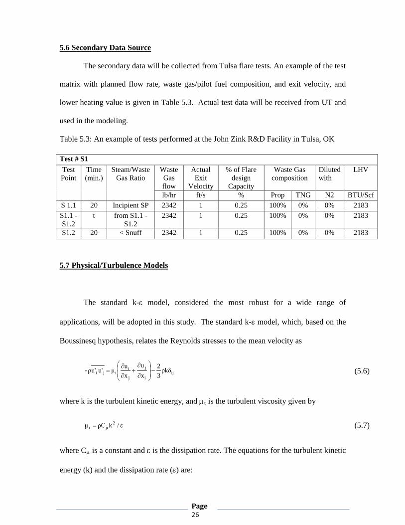
5.6 Secondary Data Source
The secondary data will be collected from Tulsa flare tests. An example of the test
matrix with planned flow rate, waste gas/pilot fuel composition, and exit velocity, and
lower heating value is given in Table 5.3. Actual test data will be received from UT and
used in the modeling.
Table 5.3: An example of tests performed at the John Zink R&D Facility in Tulsa, OK
Test # S1 Test Point
Time (min.)
Steam/Waste Gas Ratio
Waste Gas flow
Actual Exit
Velocity
% of Flare design
Capacity
Waste Gas composition
Diluted with
LHV
lb/hr ft/s % Prop TNG N2 BTU/Scf S 1.1 20 Incipient SP 2342 1 0.25 100% 0% 0% 2183 S1.1 - S1.2
t from S1.1 - S1.2
2342 1 0.25 100% 0% 0% 2183
S1.2 20 < Snuff 2342 1 0.25 100% 0% 0% 2183
5.7 Physical/Turbulence Models
The standard k-ε model, considered the most robust for a wide range of
applications, will be adopted in this study. The standard k-ε model, which, based on the
Boussinesq hypothesis, relates the Reynolds stresses to the mean velocity as
iji
j
j
itji ρkδ
32
xu
xuμu'u'ρ- −
∂
∂+
∂∂
= (5.6)
where k is the turbulent kinetic energy, and µt is the turbulent viscosity given by
ε/kρCμ 2μt = (5.7)
where Cµ is a constant and ε is the dissipation rate. The equations for the turbulent kinetic
energy (k) and the dissipation rate (ε) are:
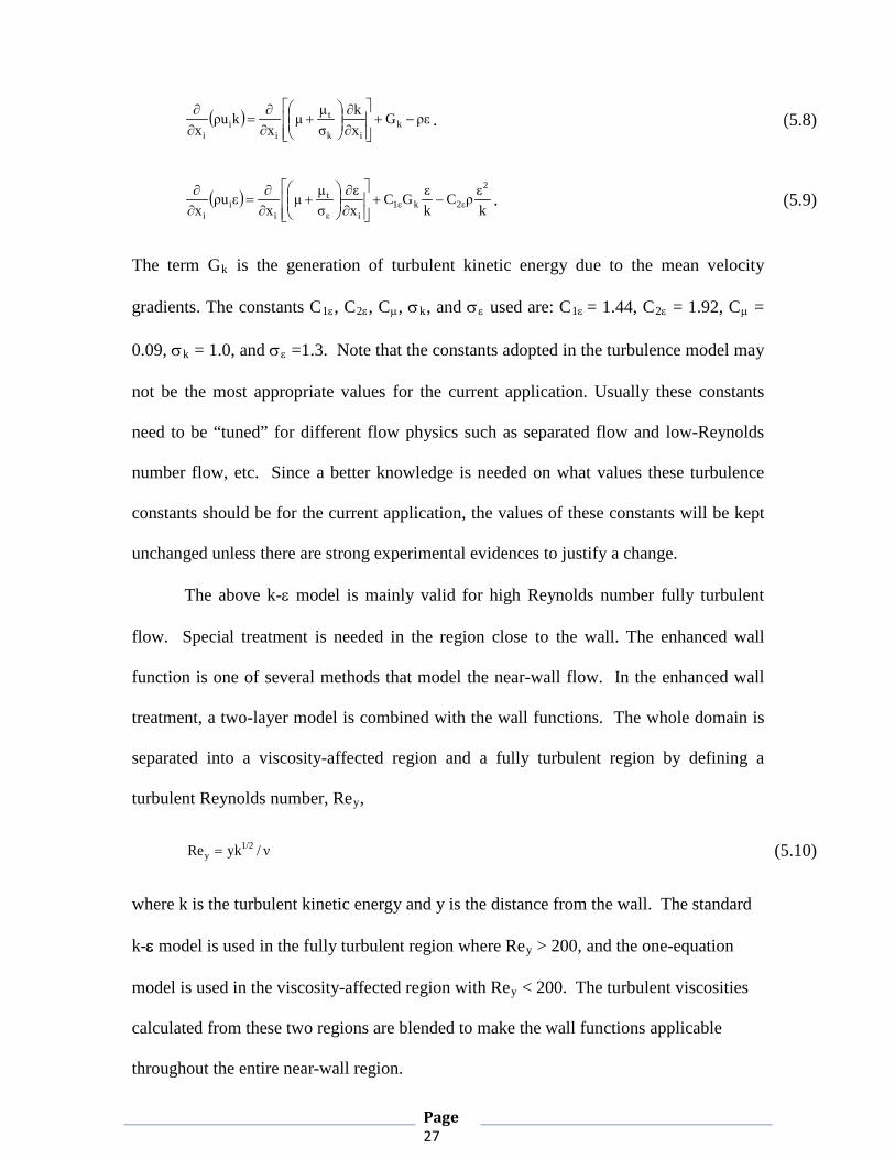
Page 27
( ) ρεGxk
σμμ
xkρu
x kik
t
ii
i−+
∂∂
+
∂∂
=∂∂ . (5.8)
( )kερC
kεGC
xε
σμμ
xερu
x
2
2εk1εiε
t
ii
i−+
∂∂
+
∂∂
=∂∂ . (5.9)
The term Gk is the generation of turbulent kinetic energy due to the mean velocity
gradients. The constants C1ε, C2ε, Cµ, σk, and σε used are: C1ε = 1.44, C2ε = 1.92, Cµ =
0.09, σk = 1.0, and σε =1.3. Note that the constants adopted in the turbulence model may
not be the most appropriate values for the current application. Usually these constants
need to be “tuned” for different flow physics such as separated flow and low-Reynolds
number flow, etc. Since a better knowledge is needed on what values these turbulence
constants should be for the current application, the values of these constants will be kept
unchanged unless there are strong experimental evidences to justify a change.
The above k-ε model is mainly valid for high Reynolds number fully turbulent
flow. Special treatment is needed in the region close to the wall. The enhanced wall
function is one of several methods that model the near-wall flow. In the enhanced wall
treatment, a two-layer model is combined with the wall functions. The whole domain is
separated into a viscosity-affected region and a fully turbulent region by defining a
turbulent Reynolds number, Rey,
ν/ykRe 1/2y = (5.10)
where k is the turbulent kinetic energy and y is the distance from the wall. The standard
k-ε model is used in the fully turbulent region where Rey > 200, and the one-equation
model is used in the viscosity-affected region with Rey < 200. The turbulent viscosities
calculated from these two regions are blended to make the wall functions applicable
throughout the entire near-wall region.
Page 28
6. PROJECT QUALITY METRICS
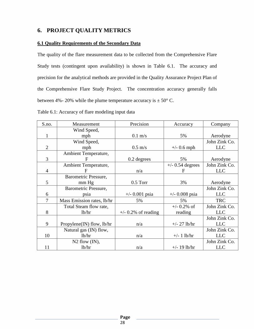
6.1 Quality Requirements of the Secondary Data
The quality of the flare measurement data to be collected from the Comprehensive Flare
Study tests (contingent upon availability) is shown in Table 6.1. The accuracy and
precision for the analytical methods are provided in the Quality Assurance Project Plan of
the Comprehensive Flare Study Project. The concentration accuracy generally falls
between 4%- 20% while the plume temperature accuracy is ± 50° C.
Table 6.1: Accuracy of flare modeling input data
S.no. Measurement Precision Accuracy Company
1 Wind Speed,
mph 0.1 m/s 5% Aerodyne
2 Wind Speed,
mph 0.5 m/s +/- 0.6 mph John Zink Co.
LLC
3 Ambient Temperature,
F 0.2 degrees 5% Aerodyne
4 Ambient Temperature,
F n/a +/- 0.54 degrees
F John Zink Co.
LLC
5 Barometric Pressure,
mm Hg 0.5 Torr 3% Aerodyne
6 Barometric Pressure,
psia +/- 0.001 psia +/- 0.008 psia John Zink Co.
LLC 7 Mass Emission rates, lb/hr 5% 5% TRC
8 Total Steam flow rate,
lb/hr +/- 0.2% of reading +/- 0.2% of
reading John Zink Co.
LLC
9 Propylene(IN) flow, lb/hr n/a +/- 27 lb/hr John Zink Co.
LLC
10 Natural gas (IN) flow,
lb/hr n/a +/- 1 lb/hr John Zink Co.
LLC
11 N2 flow (IN),
lb/hr n/a +/- 19 lb/hr John Zink Co.
LLC
Page 29
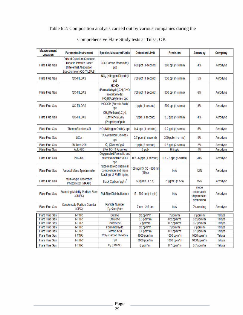
Table 6.2: Composition analysis carried out by various companies during the
Comprehensive Flare Study tests at Tulsa, OK
Page 30

Page 31

Page 32
6.2 CFD Model Uncertainty
The USC and GRI mechanisms used in conjunction with CHEMKIN CFD and
FLUENT are all in good agreement with the laboratory experimental data13. Even so,
the uncertainty of measurements (listed for individual species and CE/DRE in
Comprehensive flare test QAPP and report) are somewhat smaller than the uncertainty of
the combined USC/GRI mechanism20,21, which ranges from a factor of 1.2 to 5 for trace
species. and in the order of ± 4% (for CO2) to ±15% (for NO) for major species, Table
6.3. The mechanism uncertainty factor depends on residence, temperature, fuel
composition, species, etc. Fortunately, these mechanism parameters have been optimized
with lab data, mostly within experimental errors. For the sake of simplicity, a typical
uncertainty factor of 2 will be used for trace species (in ppm range). A factor of 2 means
the true value could lie from 0.5* model value to 2*model value. For major species, in
general, these mechanisms can reflect lab data within ± 10% for CO, within ±15% for
NO based on GRI’s assessment and are generally accepted in the combustion chemistry
community.
Recent simulations suggest that the uncertainty in transport coefficients may be
significant. As a result, the uncertainty factor of 3 will be used for the trace species.
CE/DRE Prediction Uncertainty
For relation DCA /= , uncertainty is calculated using
DdDCdCAdA /// +=
The above formula states that the uncertainty (in percentage) of A is the sum of the
uncertainty of C (in percentage) and the uncertainty of D (in percentage).
Page 33
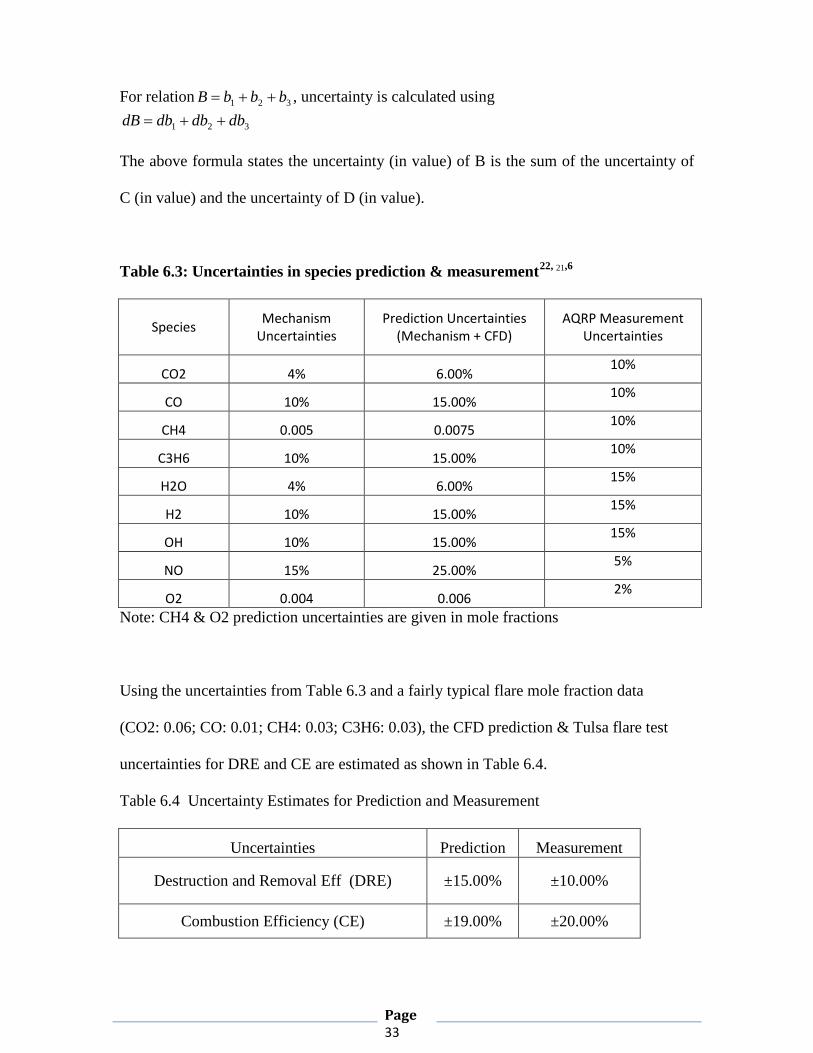
For relation 321 bbbB ++= , uncertainty is calculated using
321 dbdbdbdB ++=
The above formula states the uncertainty (in value) of B is the sum of the uncertainty of
C (in value) and the uncertainty of D (in value).
Table 6.3: Uncertainties in species prediction & measurement22, 21,6
Species Mechanism Uncertainties
Prediction Uncertainties (Mechanism + CFD)
AQRP Measurement Uncertainties
CO2 4% 6.00% 10%
CO 10% 15.00% 10%
CH4 0.005 0.0075 10%
C3H6 10% 15.00% 10%
H2O 4% 6.00% 15%
H2 10% 15.00% 15%
OH 10% 15.00% 15%
NO 15% 25.00% 5%
O2 0.004 0.006 2%
Note: CH4 & O2 prediction uncertainties are given in mole fractions
Using the uncertainties from Table 6.3 and a fairly typical flare mole fraction data
(CO2: 0.06; CO: 0.01; CH4: 0.03; C3H6: 0.03), the CFD prediction & Tulsa flare test
uncertainties for DRE and CE are estimated as shown in Table 6.4.
Table 6.4 Uncertainty Estimates for Prediction and Measurement
Uncertainties Prediction Measurement
Destruction and Removal Eff (DRE) ±15.00% ±10.00%
Combustion Efficiency (CE) ±19.00% ±20.00%

Page 34
For CO, the measurement uncertainty is ±15% (IMACC) and the model uncertainty is
±15% (Mechanism +Fluid Dynamics), then the acceptance criterion is ±30%.
7. DATA ANALYSIS, INTERPRETATION AND MANAGEMENT
7.1 Cross-Project Review by Air Quality Research Program (AQRP)
Stage 1 – After the model has been developed and before any simulations are run, the
Principal Investigator shall provide a presentation to the AQRP Project Manager and
Staff to review the model development. This review will focus on, but not be limited to,
the inputs and assumptions used in the development of the model and verify the specific
base case (to be specified by the AQRP Project Manager) that will be used for inter-
comparison of the flare CFD models. No further work shall be performed on this project
until Stage 1 approval has been given by the AQRP Project Manager.
Stage 2 – Upon completion of the simulations, the Principal Investigator shall provide a
presentation of the results of the base case specified in Stage 1 to the AQRP Project
Manager and Staff. This Stage 2 review is a quality assurance assessment of the
performance of the model. The Project Manager will make recommendations on
restrictions for use of the model that shall be included in the final report.
7.2 Results Comparison: CFD vs. Flare Test Data
The report will summarize the validation of analytical results generated from field
sampling at John Zink facility, Tulsa, Oklahoma. Emission rate of all monitored species
will be calculated. Whenever applicable, DRE and CE will be computed. CE, DRE and

Page 35
Species Concentration model values will be compared vs. Aerodyne, IMACC, Telops and
TRC data when available.
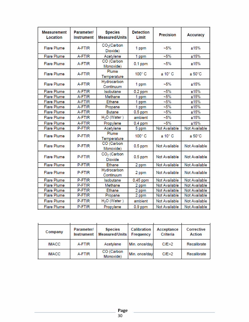
Table 7.1 below present the composition analysis carried out by Aerodyne, Telops,
and IMACCs during the TCEQ Flare tests in Tulsa.
Table: 7.1: Parameters to be compared with the Tulsa Flare Test
Species being Measured at Tulsa Are they considered in the
mechanism Aerodyne Telops TRC IMACC CO
NO2
HCHO (Formaldehyde)
CH3CHO (Acetaldehyde)
HC2H (Acetylene)
CH4
C3H6 (Propylene)
NO
CO2
EPA TO-14 ANALYTES
Oxygenated/ Aromatic and selected olefinic VOC
Ethylene (C2H4)
Water
Ethane
Propane
Page 36
8. DATA REPORTING AND QUALITY ASSURANCE & CONTROL
PROCEDURES
8.1 Data Storage & Reporting
Lamar University will simulate flaring activities with the design/operating &
meteorological data collected from the UT/TCEQ Comprehensive Flare Study Project
(PGA No. 582-8-862-45-FY09-04) as the input variables using computational fluid
dynamics (CFD) programs. The data comparison, when available, will be carried out
with model uncertainty and the measurement uncertainty in mind. The data will be stored
in external hard drives for three years. The data include various fluent case runs and excel
files containing data analysis.
8.2 Controlled Flare Test Data
Measurement uncertainty mainly depends on accuracy: generally between 4%-20%
for concentrations and ± 50° C for temperatures, Table 6.2.
8.3 Mechanism & Fluid Dynamics Uncertainties
The USC and GRI mechanisms used in conjunction with CHEMKIN CFD and
FLUENT are all evaluated based on the performance of the laboratory experimental
dataError! Bookmark not defined.. In general, these mechanisms can reflect lab data
within ± 10% for CO, within ±15% for NO based on GRI’s assessment and are generally
accepted in the combustion chemistry community. For trace species and fluid dynamics
model uncertainties, see Sec. 6.2.
Recent simulations suggest that the uncertainty in transport coefficients may be
significant. As a result, the uncertainty factor of 3 will be used for the trace species and
Page 37
the uncertainty factor in Table 6.3 should be multiplied by 1.5 after considering both
mechanism and fluid dynamics uncertainty factors20.
8.4 Quality Assurance/Quality Control Procedures
The QA/QC activities include Project Management, Project Data Acquisition,
Project Assessment/Oversight, and Data Validation and Usability Test1. All of the
developed models, computational programs and project data will be saved to CDs and
removable hard drives regularly for long-term storage. The computers will be well
maintained and subject to the lab safety rules at Lamar University. Project progress will be
internally reviewed by the research group every week. The PI/Co-PIs will carefully
supervise these activities. Each task contains quality assurance/quality control provisions
that involve works being reviewed and checked by PI/Co-PIs and the UT representative
Vincent Torres.
FLUENT/CHEMKIN Simulated results will be rigorously checked for numerical
convergence and elemental mass balance. Field or test flare data will be checked for
accuracy for numerical data entry, unit consistency, and mass balance. The uncertainties
involved in numerical simulations and field data (measurements) will be evaluated and
reflected in all model building. The actual project progress will be checked against the tasks
listed in the proposed milestone chart and the reason for delays, if any, will be documented.
Based on the progress, two to three journal or conference papers are expected to be
generated. The research achievements will also be parts of the theses of the research
associates. The PI/Co-PIs will supervise these activities. Since no experiments will be
performed, the safety of those working on the project will not be affected.
Page 38
9. REFERENCES
1 Quality Assurance/Quality Control Plan, Quality Assurance Project Plan (QAPP) for Gulf Coast Hazardous Substance Research Center (GCHSRC), Project Number 027LUB0599, June, 1998. 2 Flare efficiency study,EPA-600/2-83-052, Marc Daniel, July 1983 3 J.H. Pohl, Evaluation of the Efficiency of Industrial Flares, 1984/1985, EPA600-2-85-95 and 106 4 David Castiñeira and Thomas F. Edgar, Computational Fluid Dynamics for Simulation of Wind-Tunnel Experiments on Flare Combustion Systems, Energy & Fuels 2008, 22, 1698–1706 5 Passive FTIR Phase I Testing of Simulated and Controlled Flare Systems, FINAL REPORT, (URS/UH/TCEQ, 2004) (http://www.tceq.state.tx.us/assets/public/implementation/air/am/contracts/reports/oth/Passive_FTIR_PhaseI_Flare_Testing_r.pdf) 6 Quality Assurance Project Plan, Texas Commission on Environmental Quality Comprehensive flare Study Project, PGA No. 582-8-862-45-FY09-04, Tracking No. 2008-81 UT/TCEQ/John Zink) 7 Sharma, R., “State of the Ozone State Implementation Plan” Proceeding of Ethylene Producers Conference, pp 392-397, AIChE Spring Houston Meeting 2007 8 Daniel J.Serry, C.T.Bowman, "An Experimental and Analytical Study of Methane Oxidation behind Shock Wavess",Combustion and Flame ,14,37-48(1970). 9 Seinfeld, John H. ; Pandis, Spyros, 2006. Atmospheric Chemistry and Physics - From Air Pollution to Climate Change, 2nd edition John Wiley & Sons 10 US EPA, Office of Air Quality Planning and Standards, Quality Assurance Handbook for Air Pollution Measurement Systems, EP-454/R-98-004, August 1998. 11 URS Corporation. (2004) Passive FTIR Phase I Testing of Simulated and Controlled Flare Systems final report, for Texas Commission on Environmental Quality and University of Houston. 12 Kostiuk, L, Johnson, M and Thomas, G. (2004). University of Alberta Flare Research Project Final Report. 13 David Castiñeira and Thomas F. Edgar, “CFD for Simulation of Steam-Assisted and Air-Assisted Flare Combustion Systems”, Energy & Fuels 20, 1044-1056 (2006) 14 Ferziger, J.H.; Peric, M. Computational Methods for Fluid Dynamics; 3rd edition; Springer: Berlin, 2002
Page 39
15 Tomlin, A.; Pilling, M.; Turányi, T.; Merkin, J.; Brindley, J. Mechanism Reduction for the Oscillatory Oxidation of Hydrogen: Sensitivity and Quasi-Steady-State Analysis. Combust. Flame 1992, 91, 107-130 16 Anjan Tula, CFD Model for Validation of a Combustion Mechanism for Light Hydrocarbons, Master’s thesis, August, 2010, Lamar University, Beaumont, TX. 17 C.K.Law , A.Makino , and T.F.Lu, "On the Off-Stoichiometric Peaking of Adiabatic Flame Temperature ", The 4th J. Meeting of the U.S. Sections of the Combustion Institute,#1844(Mar 2005) 18 Qin.Z, Yang.H, C.Gardiner, " Measurement and modeling of shock-tube ignition delay for propene ", Combustion and Flame ,124, 246-254 (2001) 19 ANSYS Inc., ANSYS 13, User’s Guide. Fluent Inc (2010) 20 David A. Sheen, Xiaoqing You, Hai Wang, Terese Lovas, Spectral uncertainty quantification, propagation and optimization of a detailed kinetic model for ethylene combustion, Proceedings of the Combustion Institute, 32(1), 2009, 535-542 21 Hai Wang, Xiaoqing You, Ameya V. Joshi, Scott G. Davis, Alexander Laskin, Fokion Egolfopoulos & Chung K. Law, USC Mech Version II. High-Temperature Combustion Reaction Model of H2/CO/C1-C4 Compounds. http://ignis.usc.edu/USC_Mech_II.htm, May 2007 22 R.S.Barlow,A.N.Karpetis, J.H.Frank, J.Y. Chen,”Scalar Profiles and NO formation in laminar opposed flow partially premixed methane/air flames” Combustion and flame(2001),