quality and reliability of elastomer sockets
TRANSCRIPT

ABSTRACT
Title of Document: QUALITY AND RELIABILITY OF
ELASTOMER SOCKETS Leoncio D. Lopez, Doctor of Philosophy
(Ph.D.), 2009 Directed By: Chair Professor and Director, Michael G. Pecht,
Department of Mechanical Engineering
Integrated Circuit (IC) sockets provide hundreds to thousands of electrical
interconnects in enterprise servers, where quality and reliability are critical for
customer applications. The evaluation of IC sockets, according to current industry
practices, relies on the execution of stress loads and stress levels that are defined by
standards, having no consideration to the physics of failure (PoF), target operating
environment, or contact resistance behavior over time. In a similar manner,
monitoring of contact resistance during system operation has no considerations to the
PoF or environmental conditions.
In this dissertation a physics of failure approach was developed, to model the
reliability of elastomer sockets that are used in an enterprise server application. The
temperature and relative humidity environment, at the IC socket contact interface,
were characterized as a function of external environmental conditions and
microprocessor activity. The study applied state-of-the-art health monitoring

techniques to assess thermal gradients on the IC socket assembly, and to establish an
operating profile that could be used for the development of a PoF model.
A methodology was developed for modeling and monitoring contact
resistance of electrical interconnects. The technique combined a PoF model with the
Sequential Probability Ratio Test (SPRT). In the methodology the resistance behavior
is characterized as a function of temperature. The effective a-spot radius was
extracted from the characterization data and modeled with a power-law. A PoF model
was developed to estimate the resistance of an elastomer contact, based on the
effective a-spot radius and the ambient temperature. The methodology was
experimentally demonstrated with a temperature cycle test of the elastomer socket.
During the evaluation the difference between estimated and observed resistance
values were tested with the SPRT. The technique was shown to be very accurate for
modeling contact resistance, and to be highly sensitive for the detection of resistance
degradation.
A qualitative reliability model was developed for the mean contact resistance
of an elastomer socket, using fundamental material properties and user defined failure
criteria. To derive the model, the resistance behavior of contacts under nominal
mechanical load was studied as a function of time and temperature. The elastomer
contact was shown to have a very complex resistance behavior, which was modeled
by multiple statistical distributions. It was shown that elastomer sockets, in spite of
experiencing stress relaxation at the macroscale (elastomer), can exhibit decreases in
contact resistance, a result of stress redistribution at the microscale (Ag particles),
which increases Ag-Ag particle stress and the effective contact area.

QUALITY AND RELIABILITY OF ELASTOMER SOCKET
By
Leoncio D. Lopez
Dissertation submitted to the Faculty of the Graduate School of the University of Maryland, College Park, in partial fulfillment
of the requirements for the degree of Doctor of Philosophy
2009 Advisory Committee: Professor Michael G. Pecht, Chair Professor Donald Barker Associate Professor Peter Sandborn Associate Professor David Bigio Professor Herbert Rabin, Dean’s Representative

© Copyright by Leoncio D. Lopez
2009

Preface
“In the discovery of secret things, and in the investigation of hidden causes,
stronger reasons are obtained from sure experimentations and demonstrated
arguments, than from probable conjectures and the opinions of philosophical
speculators.”
- William Gilbert
ii

Dedication
This is dedicated to my dear wife Cindy, and to my children Paige, Adriana,
and Braeden. Cindy’s support, patience, and continuous encouragement will never be
forgotten. There is no doubt that the sacrifices made by my family made this research
possible.
This work is also dedicated to my father, Leoncio Lopez, and my mother,
Rebeca Lopez. They taught me well as a child the value of an education.
iii

Acknowledgements
My sincere gratitude goes to Dr. Michael Pecht, my advisor, for his support
and guidance throughout my academic endeavor.
I wish to thank Dr. Abhijit Dasgupta and Dr. Donald Barker for attending my
presentations, reviewing my research plans, and providing so many valuable
suggestions. I am also very grateful to Dr. Diganta Das for his constant support.
I appreciate all of the technical reviews, critique, and suggestions that were
provided by the CALCE team members, in particular, Vidyu Challa, Sony Mathew,
Dr. Hao Yu, Weiquiang Wang, and Shunfeng Cheng.
Many thanks to Dr. David McElfresh and Dr. Kenny Gross from Sun
Microsystems for the extensive discussions, suggestions, and technical reviews. Also
thanks to Roger Blythe and Dr. Kalyan Vaidyanathan for the Sun Fire™ hardware and
software support. I am also grateful for Myra Torres’ review of my technical
presentations and for her suggestions on how to improve my work.
Special thanks to Dr. Roland Timsit, from Timron Advanced Connector
Technologies, for his invaluable training on electrical contacts.
iv

Table of Contents Preface........................................................................................................................... ii Dedication .................................................................................................................... iii Acknowledgements...................................................................................................... iv Table of Contents.......................................................................................................... v List of Tables .............................................................................................................. vii List of Figures ............................................................................................................ viii Chapter 1: Reliability of IC Sockets ............................................................................. 1
1.0 Introduction................................................................................................... 1 1.1 Motivation for Research ............................................................................... 1 1.2 Objectives of Thesis...................................................................................... 2 1.3 Overview of Thesis ....................................................................................... 2
Chapter 2: Assessing the Operating Temperature and Relative Humidity Environment of IC Sockets in Enterprise Servers .............................................................................. 4
2.0 Introduction................................................................................................... 4 2.1 Contact Resistance Distribution.................................................................... 5 2.2 Health Monitoring and Electronic Prognostics............................................. 7 2.3 Experimental Setup....................................................................................... 8 2.4 Experimental Results .................................................................................. 11
2.4.1 Temperature and Relative Humidity Profile for Power-on Transitions 11 2.4.2 Temperature Profile of Microprocessor Assembly During Server Operation13 2.4.3 Relative Humidity Profile Induced by Microprocessor ...................... 15 2.4.4 Temperature and Relative Humidity Profile of the Data Center ........ 16
2.5 Conclusions................................................................................................. 17 Chapter 3: Modeling of IC Socket Contact Resistance for Reliability and Health Monitoring Applications............................................................................................. 19
3.0 Introduction................................................................................................. 19 3.1 Introduction to the Sequential Probability Ratio Test................................. 20 3.2 Methodology............................................................................................... 24
3.2.1 Resistance Characterization ................................................................ 26 3.2.2 Physics of Failure Model Selection .................................................... 26 3.2.3 Model Validation ................................................................................ 27 3.2.4 SPRT Definition and Training ............................................................ 27 3.2.5 Resistance Monitor ............................................................................. 28
3.3 Experimental Demonstration ...................................................................... 29 3.3.1 Experimental Setup............................................................................. 29 3.3.2 Resistance Characterization ................................................................ 31 3.3.3 Physics of Failure Model Selection .................................................... 31 3.3.5 SPRT Definition and Training ............................................................ 35 3.3.6 Resistance Monitor ............................................................................. 36
3.4 Conclusions................................................................................................. 38
v

Chapter 4: Assessing the Reliability of Elastomer Sockets in Temperature Environments .............................................................................................................. 40
4.0 Introduction................................................................................................. 40 4.1 Contact Resistance Distribution.................................................................. 43 4.2 Experimental Setup..................................................................................... 43
4.2.1 Hardware............................................................................................. 43 4.2.2 Experimental Groups .......................................................................... 46 4.2.3 Test Procedure .................................................................................... 47
4.3 Results and Discussion ............................................................................... 48 4.3.1 Resistance Behavior............................................................................ 48 4.3.2 Time-Dependent Model for Mean Contact Resistance....................... 54 4.3.3 Contact Reliability .............................................................................. 57
4.4 Conclusions and Recommendations ........................................................... 58 Chapter 5: Effects of Electrical Bias on Contact Resistance ..................................... 61
5.0 Introduction................................................................................................. 61 5.1 Experimental Setup..................................................................................... 61 5.2 Results and Discussion ............................................................................... 63 5.3 Conclusion .................................................................................................. 64
Chapter 6: Sources of Failure in IC Socket Contacts ................................................ 65 6.0 Introduction................................................................................................. 65 6.1 Design ......................................................................................................... 66 6.2 Manufacturing............................................................................................. 71 6.3 System Assembly........................................................................................ 72 6.4 System Storage and Transportation ............................................................ 73 6.5 System Operation........................................................................................ 74 6.6 System Service and Repair ......................................................................... 75 6.7 Conclusions................................................................................................. 76
Chapter 7: Contributions and Future Work ............................................................... 77 7.0 Contributions............................................................................................... 77 7.1 Future Work ................................................................................................ 79
7.1.1 Socket Reliability Modeling ............................................................... 79 7.1.2 Long Term Reliability of Elastomer Sockets...................................... 80
Appendix I – Main Physical and Material Properties of the Elastomer Socket.......... 81 Appendix II – Analysis of Mechanical Load Applied to IC Socket Assemblies........ 83 Appendix III – Package and Bolster Plate Shape Analysis ........................................ 85 Appendix IV – Sensitivity Analysis of PoF Model Parameters and Model Accuracy Evaluation ................................................................................................................... 86 Appendix V – Physical Location of Test Contacts in Daisy Chain Package.............. 89 Appendix VI – Generalization of the PoF Model....................................................... 90 Bibliography ............................................................................................................... 92
vi

List of Tables Table 1. Recorded temperatures during the experiment ............................................. 14 Table 2. Resistance values from characterization test ................................................ 31 Table 3. PoF parameters for test samples ................................................................... 33 Table 4. Average temperature gradients for contacts at the maximum cyclic temperature ................................................................................................................. 34 Table 5. Resistance monitor results of sample 5......................................................... 37 Table 6. Contact resistance monitor results for temperature cycle test ...................... 38 Table 7. Sample sizes for experimental test groups.................................................... 47 Table 8. Mean contact resistance for test group data.................................................. 54 Table 9. Parameters for PoF model – three groups..................................................... 56 Table 10. Estimated reliability for first year under non-bias conditions .................... 57 Table 11. Test cells and sample sizes for electrical bias experiment.......................... 62 Table 12. Electrical bias test results............................................................................ 64 Table 13. Design factors that can induce socket failure ............................................. 70 Table 14. Manufacturing factors that can induce socket failure................................. 71 Table 15. System assembly factors that can induce socket failure ............................. 72 Table 16. System storage and transportation factors that can induce socket failure .. 73 Table 17. Operating environment factors that can induce socket failure ................... 74 Table 18. System service and repair factors that can induce socket failure ............... 75 Table 19. Main characteristics of the elastomer socket used in the research ............. 81 Table 20. Results of mechanical load analysis ........................................................... 84
vii

List of Figures Figure 1. Tyco 1.0 elastomer socket used for the experiment ...................................... 6 Figure 2. Cross-sectional illustration of an elastomer socket assembly with applied compressive load........................................................................................................... 7 Figure 3. Illustration of a microprocessor assembly used to provide compressive loads for the elastomer socket ................................................................................................ 8 Figure 4. Illustration of sensors installed on the microprocessor assembly ............... 10 Figure 5. Illustration of the server setup with data acquisition, power supply, and signal monitoring for IC sockets................................................................................. 10 Figure 6. Average temperature and relative humidity profile of the IC socket contact interface in a power-on transition ............................................................................... 12 Figure 7. Temperature signals of three microprocessors monitored by the CSTH during a ten-hour period.............................................................................................. 14 Figure 8. The temperature (°C, represented by the upper signals) and relative humidity (%, represented by the lower signals) at the IC socket interface for a ten-hour period are shown................................................................................................. 16 Figure 9. Temperature (ºC) and RH (%) in data center in a two-month period.......... 17 Figure 10. Potential outcomes in the evaluation of the probability ratio.................... 22 Figure 11. The M-SPRT methodology for monitoring contact resistance of electrical interconnects ............................................................................................................... 25 Figure 12. Process for the monitoring and analysis of contact resistance data during a temperature cycle test ................................................................................................. 29 Figure 13. Illustration of the daisy chain created by the test assembly and elastomer socket under compression ........................................................................................... 30 Figure 14. Illustration of the load assembly components used for the experiment .... 44 Figure 15. Illustration of an elastomer socket showing the 37 x 37 array of contacts, Kapton film (dark regions between contacts), and thermoplastic housing (perimeter)..................................................................................................................................... 45 Figure 16. Illustration of a two-contact chain formed by the test assembly and the IC socket .......................................................................................................................... 45 Figure 17. Three population mixed-Weibull probability plot for resistance of elastomer contacts evaluated with 25 ºC condition .................................................... 49 Figure 18. Log-normal probability plot for elastomer contact resistance evaluated with 55 ºC condition ................................................................................................... 52 Figure 19. Three-Parameter Weibull probability plot (uncorrected for gamma) for elastomer contact resistance evaluated with 75 ºC condition ..................................... 53 Figure 20. Plot for the mean contact-resistance model as a function of time for 25 ºC, 55 ºC, and 75 ºC conditions ........................................................................................ 56 Figure 21. Test circuit for bias experiment ................................................................. 62 Figure 22. Three-Parameter Weibull probability plot of control samples at 25 ºC condition ..................................................................................................................... 63 Figure 23. Sources of failure for IC socket contacts................................................... 65 Figure 24. SEM SE (20KV, 300x) image of a Cinch CIN::APSE contact................. 67
viii

ix
Figure 25. Reliability block diagram of an “x-out-of-n” system, representative of a CIN::APSE contact ..................................................................................................... 67 Figure 26. SEM BSE image (25KV, 1000x) of a Ag-filled elastomer contact cross section ......................................................................................................................... 68 Figure 27. Reliability block diagram representing an elastomer contact.................... 69 Figure 28. Series reliability model for a systems of “n” components ........................ 79 Figure 29. Illustration of elastomer socket, showing dimensions . 82 Figure 30. Illustration of elastomer contact, showing dimensions ............................. 82 Figure 31. Shadow Moiré image for sample package................................................. 85 Figure 32. Shadow Moiré image for sample bolster plate .......................................... 85 Figure 33. Sensitivity of output resistance to changes in resistivity........................... 87 Figure 34. Sensitivity of output resistance to changes in a-spot radius ..................... 88 Figure 35. Plot of resistance measurements versus model estimates, validating PoF model accuracy ........................................................................................................... 88 Figure 36. Illustration of the 37 x 37 array used in the experiment, showing the location of contacts that were monitored .................................................................... 89 Figure 37. Plot illustrating the fit of the empirical contact resistance model against measurements at 25 °C, 55 °C, and 75 °C .................................................................. 91
Chapter 1: Reliability of IC Sockets
1.0 Introduction
Enterprise servers are utilized by many corporations around the world to
handle critical software applications and data. Web portal transactions, video and
music storage, bank account management, corporate payrolls, and databases are just a
few examples. IC sockets in these enterprise servers are expected to provide the
highest levels of quality and reliability, because failure in this application
environment results in a significant loss of revenue for the customer. There are three
IC socket contact technologies that are typically used in industry: CIN::APSE (fuzz
button), stamped metal, and elastomer. Elastomer sockets in general are used because
they provide a low cost alternative and because they can be easily adapted to
practically any customer package design. However, the reliability of the elastomer
contact in server applications is not well understood. This dissertation provides a
comprehensive study of the resistance behavior of elastomer contacts, and develops
models for the estimation of contact reliability in an enterprise server application.
1.1 Motivation for Research
While many studies have been performed to analyze the properties and
behavior of the elastomer contact, there is practically no information about the actual
operating conditions at the contact interface and the long term behavior of the contact
under mechanical loads. Furthermore, there is no experimental data to define PoF
1

models that would allow the estimation of contact reliability in production
representative assemblies.
1.2 Objectives of Thesis
The main objective of this research is to define the reliability of an elastomer
contact that operates in a high-end server application. To achieve this goal the
following secondary objectives were defined: i) Identify the operating environment of
the IC socket contact; ii) Define a methodology for the detection of contact resistance
degradation; iii) Investigate the long term resistance behavior of contacts under
mechanical load; iv) Define a PoF model for the contact resistance of elastomer
sockets; v) Define the reliability of the elastomer contact in a server application.
1.3 Overview of Thesis
Quality, reliability, health monitoring, and electronic prognostic applications,
can not be successfully developed and deployed without a clear understanding of the
operating environment of the component under analysis. In Chapter 2 the temperature
and relative humidity environment for an IC socket in a high-end server application is
outlined. The experimental setup is presented, where a network of sensors and health
monitoring tools are utilized to determine operating profiles for the server,
motherboard, LGA package, IC, and socket contact interface. The relationship
between microprocessor junction temperature and contact temperature and humidity
are discussed. Temperature changes across the socket assembly are provided as a
function of microprocessor activity.
2

Chapter 3 presents a novel approach for the modeling and monitoring of
contact resistance. The technique is introduced for reliability and health monitoring
applications. A model for the true contact area radius as a function of temperature is
discussed. A model for the elastomer contact resistance is presented. The approach is
demonstrated for the estimation of contact resistance during a temperature cycle
experiment. The methodology steps and implementation are outlined.
Chapter 4 presents a study on the contact resistance behavior of elastomer
sockets as a function of time and temperature. A model for the mean a-spot radius as
a function of time is presented, and a model for the contact resistance is discussed.
The implementation of a log-normal-PoF model to estimate contact resistance during
the first year of operation is outlined. Chapter 5 discusses the effects of electrical bias
on elastomer contacts.
Chapter 6 outlines potential sources of failure in IC socket assemblies. The
differences between two contact design alternatives are described from the reliability
point of view. Other sources of failure presented include manufacturing, system
assembly, system storage and transportation, system operation, and system service
and repair. The contributions from this research, as well as suggested future work, are
provided in Chapter 7.
3

Chapter 2: Assessing the Operating Temperature and Relative Humidity Environment of IC Sockets in Enterprise Servers
2.0 Introduction
Microprocessors in high-end computer systems are typically connected to
printed circuit boards (PCB) by either solder joints or by IC sockets. IC sockets are
used as an alternative to solder joints because they can provide a repairable, heatless,
high density, and reliable interconnect solution. In some applications these sockets
provide interconnection for over 32000 power, ground, and signal lines in a single
server.
Current industry practices, such as ANSI/EIA-364 and Telcordia GR-1217-
CORE, for the evaluation of IC sockets rely on the execution of predetermined stress
loads (e.g., temperature, humidity, shock, vibration), at predetermined load intensities
without consideration to the operating conditions, IC socket characteristics, or
reliability requirements [1]-[3]. Similar methods are used for the evaluation of test
and burn-in sockets [4]. The qualification of IC sockets under current practices does
not supply the information needed to derive acceptable reliability models and
operating life estimates [5]. To assure high levels of reliability for the IC socket it is
necessary to perform tests that mimic the actual component operating environment,
providing acceleration of relevant failure mechanisms.
4
Over the socket life cycle, dust, shock, vibration, temperature, temperature
cycling, humidity, and corrosive gas exposure, can trigger failure mechanisms such as
creep, stress relaxation, contact wear, stiction, deformation, and corrosion among
others, which can result in permanent or intermittent contact resistance changes [6],
[7]. For IC sockets, temperature and humidity environmental stresses are important
drivers of failure [6]. Understanding these operating conditions, and the behavior of
the IC socket over time, is paramount for socket reliability and prognostic analysis.
Health Monitoring (HM) and Electronic Prognostics (EP) are methods of gathering
and analyzing information about a component or system during actual application
conditions, and allow the derivation of reliability models and life estimates [8].
This study evaluates the operating temperature and relative humidity
environment of an IC socket inside of an enterprise server, enabling quality,
reliability, and prognostic analyses. These parameters are monitored over three
months of normal operation. Variations during power-on transitions are characterized.
Microprocessor activity and its effect on the IC socket environment are analyzed.
Thermal profiles of the silicon die, microprocessor package, printed circuit board
(PCB), and data center are identified.
2.1 Contact Resistance Distribution
An IC socket is an electro-mechanical system that, by means of compression,
provides a separable, repairable, and solderless electrical interface between an IC
component and a PCB [6]. The IC socket is composed of a polymer housing (for
handling, physical protection, electrical isolation, load bearing and alignment), and an
5

array of contacts. Three common IC socket contact technologies are stamped metal,
fuzz button, and metal-filled elastomer. For the experiment described in this
publication Tyco 1.0 sockets were utilized. The Tyco socket is a 37 x 37 array of
silver-filled elastomer contacts that are molded onto a Kapton polyimide film and
attached to a thermoplastic housing. The socket dimensions are 55.0x57.0x3.3 mm,
excluding two alignment posts, as shown in Figure 1 (see Appendix I).
Figure 1. Tyco 1.0 elastomer socket used for the experiment. This design has 1369
contacts arranged in a 37x37 array. The socket is 55mm wide and 57mm long
When the IC socket contacts are compressed between an IC package and a
PCB, the silver particles inside the elastomer matrix touch each other, creating a
percolation network, as illustrated in Figure 2. An important characteristic of this
technology is that all metal-to-metal contacts that are created with the applied
compressive load are encapsulated by the elastomer, limiting the exposure to
contaminants and humidity in the air. A detailed analysis of the compressive load and
load distribution of IC socket assemblies is provided in [9] and [10].
6

Figure 2. Cross-sectional illustration of an elastomer socket assembly with applied
compressive load. The silver particles in the elastomer matrix contact each other and create a percolation network
2.2 Health Monitoring and Electronic Prognostics
Health Monitoring and Electronic Prognostics methods consist of the
continuous assessment of a product's operating environment and performance, to
enable the derivation of reliability models, estimates of remaining life, and detection
of deviations from expected normal operating conditions. These methods are typically
implemented in mission-critical or safety-critical systems such as aircraft, nuclear
power plants, medical equipment, military applications, and enterprise servers. HM
can be performed by means of diagnostic, prognostic, or life consumption monitors.
Diagnostic monitors determine the current state of health of a system, identifying
potential problems. Prognostic monitors analyze system health information,
estimating future reliability based on the physics of failure (PoF). Consumption
monitors measure the operating conditions and assess accumulated damage, providing
estimates of remaining life [11].
The following sections demonstrate a setup for HM of an IC socket’s
operating environment and the collection of information. The substantial data that is
7

acquired in this manner enables the identification of key failure mechanisms, the
development of accurate reliability models and quantitative qualification plans, and
the overall implementation of EP tools.
2.3 Experimental Setup
A Sun Fire™ 6800 server was used as the test vehicle to assess the operating
environment of the elastomer socket described in section 2.1. This enterprise server
has six motherboards, each one with four UltraSPARC© III microprocessors, cache
memory, DIMM, and a variety of active and passive components. The IC sockets and
microprocessors were installed above the PCB, compressing the contacts to
specification (60-80 g each) by means of a heatsink, bolster plate, springs, and
screws, reducing the average contact height from 940 μm down to 650 μm. The
microprocessor assembly is illustrated in Figure 3.
Figure 3. Illustration of a microprocessor assembly used to provide compressive
loads for the elastomer socket. The thermal interface and insulating Mylar layers are shown
8

Due to assembly space constraints it was necessary to make two modifications
to the socket housing that would allow the installation of sensors at the contact
interface. First, a small perforation was made to embed a thermocouple for the
monitoring of air temperature. Second, a cavity was made to embed a modified
Honeywell HIH-3610-004 relative humidity sensor. The sensor plastic housing was
cut and polished to a size of 6x4x1.5mm and fitted to this cavity. None of these
modifications compromised the structural integrity of the housing or contact
alignment.
Thermocouples were installed on the top surface of the microprocessor
packages and on PCB locations near the IC socket. HOBO® U10-003 data recorders
were attached to the server chassis to monitor the temperature and relative humidity
of the data center. One recorder was placed near the floor level (lower recorder) and
another near the system air intake (upper recorder), next to the motherboards. Overall
10 IC sockets, 10 microprocessors, and 3 PCBs were wired, providing 23
thermocouples, 3 internal relative humidity sensors, and 2 external temperature and
relative humidity sensors.
The Continuous System Telemetry Harness (CSTH), part of the Sun Fire™
server, was used to monitor the junction temperature of all 24 microprocessors. The
CSTH manages a sensor network, allowing the capture, conditioning, synchronizing,
and storage of telemetry signals for later use by HM and EP applications [13].
An Agilent E3643A DC power supply was used to power the humidity
sensors and a HP 34970A data acquisition/switch was used to measure the
9

thermocouple and humidity sensor outputs. Both instruments were controlled by
means of a computer, a GPIB (IEEE 488) interface card, and a C-language program.
The temperature and humidity sensors were monitored at five-minute intervals. The
microprocessor temperature was monitored at one-minute intervals. The setup for the
microprocessor assembly and server are illustrated in Figures 4 and 5.
Figure 4. Illustration of sensors installed on the microprocessor assembly.
Thermocouples are placed on the socket, package and PCB. A relative humidity sensor is placed in the socket housing, above the Kapton carrier. Bolster plate, springs, screws,
and other assembly components not shown for clarity
DataAcquisition
ComputerServer
PowerSupply
GPIB1 2 3 4 5 6
Boards
Figure 5. Illustration of the server setup with data acquisition, power supply, and
signal monitoring for IC sockets. The CSTH functions are integrated into the server and not shown
10

The sensor network and the CSTH were tested and calibrated over a three-day
period with power-on and power-off conditions. The temperature and relative
humidity of the air entering the system, while the motherboard power was off (system
fans on), were compared with measurements from sensors at the IC socket contact
interface. When the sensor and system calibration was completed the experiment was
initiated. The microprocessor executed a Linpack-based script with two-hour cycles
(one hour idle, one hour running the benchmark test), simulating server demand
during operation. The experiment was carried out for three months inside a data
center located in San Diego, CA.
2.4 Experimental Results
2.4.1 Temperature and Relative Humidity Profile for Power-on Transitions
The first activity in this experiment was the monitor of temperature and
relative humidity during power-on transitions. With the motherboards powered-off
and the cooling fans operating to provide airflow, the temperature and relative
humidity at the socket interface was allowed to stabilize and match those of the data
center, as indicated by the HOBO® recorders. After four hours all motherboards were
powered-on, initializing the operating system and test script for each microprocessor.
The effects of this power-on transition on the operating environment of the IC socket
are shown in Figure 6.
11

Figure 6. Average temperature and relative humidity profile of the IC socket contact
interface in a power-on transition
As the microprocessor junction temperature increased, the relative humidity at
the socket interface decreased significantly, from a 49%RH average (45-52% range)
down to 24%RH (22-28% range), all in the course of one hour. In the same period of
time the air temperature at the socket interface increased from a 22 °C average (21-23
°C range) up to 41 °C (38-45 °C range). Evaluations performed for automotive
assemblies have measured similar shifts in temperature and relative humidity inside
enclosed connectors [14].
An important observation from this data is the change in temperature and
relative humidity ranges after the system power is turned on. When the
microprocessor temperature stabilizes, relative humidity readings at the socket
contact interface are more stable, changing only by 2-3% on any given signal. The
same is true for the air temperature, which shows less than 3 °C variation over time.
12

In the experiment it was also observed that three temperature measurements were
consistently higher than other measurements. These signals were found to be
monitoring microprocessors on motherboards at the edge of the system, next to the
chassis (labeled as 1 and 6 in Figure 5).
While an increase in temperature and a reduction in relative humidity are
expected inside electronic assemblies in normal operation, the magnitude of change
and correlations with external environmental variables were unknown for the IC
socket contact interface. For some IC socket technologies, such as those that utilize
stamped metal contacts, temperature and humidity are key drivers of corrosion and
fretting mechanisms [15]. Having accurate information about the actual operating
environment allows better and more realistic reliability evaluations and enables EP
implementations [16], [17].
2.4.2 Temperature Profile of Microprocessor Assembly During Server Operation
The temperature profile of three microprocessors over a ten-hour period is
shown in Figure 7. Each one of the temperature signals cycled every two hours. The
lower temperatures were reached when the microprocessor was idle. The higher
temperatures were reached when the microprocessor was executing benchmark tests.
The observed variability at each one of the temperature levels was caused by low
resolution sensors in the microprocessor, which can only detect changes greater than
1 °C. The recorded temperatures of the microprocessor die, microprocessor packages,
socket contact (air), and PCBs are summarized in Table 1.
13
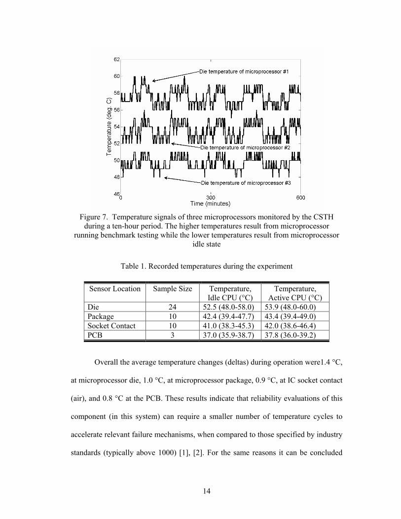
Figure 7. Temperature signals of three microprocessors monitored by the CSTH
during a ten-hour period. The higher temperatures result from microprocessor running benchmark testing while the lower temperatures result from microprocessor
idle state
Table 1. Recorded temperatures during the experiment
Sensor Location Sample Size Temperature, Idle CPU (°C)
Temperature, Active CPU (°C)
Die 24 52.5 (48.0-58.0) 53.9 (48.0-60.0) Package 10 42.4 (39.4-47.7) 43.4 (39.4-49.0) Socket Contact 10 41.0 (38.3-45.3) 42.0 (38.6-46.4) PCB 3 37.0 (35.9-38.7) 37.8 (36.0-39.2)
Overall the average temperature changes (deltas) during operation were1.4 °C,
at microprocessor die, 1.0 °C, at microprocessor package, 0.9 °C, at IC socket contact
(air), and 0.8 °C at the PCB. These results indicate that reliability evaluations of this
component (in this system) can require a smaller number of temperature cycles to
accelerate relevant failure mechanisms, when compared to those specified by industry
standards (typically above 1000) [1], [2]. For the same reasons it can be concluded
14

that accelerated temperature storage tests can be more effective in simulating normal
operating conditions for this application. The microprocessor, package, socket, and
PCB temperature signals could be used by EP tools to detect thermal anomalies and
to estimate stresses in the assembly induced by temperature gradients and temperature
cycling. Tools such as the Multivariate State Estimation Technique (MSET) and
Sequential Probability Ratio Test (SPRT) can be used to detect the incipience of
failures, aid in the identification of root causes of failure, and reduce No Trouble
Found (NTF) events [11], [12].
2.4.3 Relative Humidity Profile Induced by Microprocessor
The temperature and relative humidity measured at the IC socket interface for
a ten-hour period is shown in Figure 8. The temperature, represented by the signals at
the top of the figure, was on average 41.0 °C (38.3 to 45.3 range) when the
microprocessor was idle and 43.4 °C (39.4 to 49.0 range) when the microprocessor
was executing benchmark tests. Under the same conditions the relative humidity,
represented by the signals at the bottom of Figure 8, was on average 24.0% (21.7 to
27.3% range, idle) and 23.3% (20.8 to 27.3% range, running benchmark tests). The
cyclic changes in socket ambient temperature result in less than 3% variation in the
relative humidity. For the samples monitored, and within the temperature range
considered for this study, a 0.8% reduction in relative humidity can be expected for
every 1 °C increase in temperature. The relative humidity and temperature monitor
data, as illustrated in Figure 8, could be used by EP tools to estimate corrosion rates
of metal connectors, degradation of materials over time, and occurrence of
temperature and humidity accelerated events.
15

Figure 8. The temperature (°C, represented by the upper signals) and relative
humidity (%, represented by the lower signals) at the IC socket interface for a ten-hour period are shown. Corresponding microprocessor temperatures for the same
period are shown in Figure 7
2.4.4 Temperature and Relative Humidity Profile of the Data Center
The temperature and relative humidity of the data center environment for a
two-month period is illustrated in Figure 9. The temperature was 21.6 °C average
(20.4-24.4 °C) with relative humidity at 45.6% average (32.2-54.1%). The measured
temperatures were consistent with those expected of computer rooms but the relative
humidity was at times above the suggested range of 45-55% [18].
16

Figure 9. Temperature (ºC) and RH (%) in data center in a two-month period
These results were obtained with the HOBO® recorder located next to the
motherboards (upper recorder). Similar measurements were obtained with the
recorder located near the floor level (lower recorder). Temperatures at the upper
recorder were found to be on average 1 °C higher and relative humidity 3% lower
than those obtained by the lower recorder. These differences are caused by the heat
generated by the servers in the data center.
2.5 Conclusions
In this paper the temperature and relative humidity environment of an IC
socket inside an enterprise server was evaluated. The environment, at the socket
contact interface, was characterized during power-on transitions and monitored
during normal operating conditions. The temperature of the microprocessor die,
packages, PCBs, and data center were measured for the duration of the test. The
17

relative humidity in the data center was also monitored. The microprocessor die
temperature was found to be on the average 53 °C (48-60 °C range), which resulted in
41 °C and 23% relative humidity at the contact interface. The variation in temperature
and relative humidity during operation was found to be less than 3 °C and 3%
respectively. For the temperature range considered in this experiment, and for this
server application, the relative humidity can be expected to decrease 0.8% for every 1
°C increase in temperature. The relative humidity at the IC socket interface was found
to be 25-30% lower than that of the data center environment. The data suggests that,
for this particular server application, temperature storage tests can be optimal toward
accelerating the non-bias operating environment of the socket. In addition, given the
relatively benign temperature cycle profile, short temperature cycle evaluations
(<1000 cycles) should be considered to simulate power cycle, temperature cycle, and
interconnect aging.
The temperature and relative humidity profiles identified in this experiment
can be used with physics of failure models to assess the interconnect reliability, to
determine what failure mechanisms are relevant for the operating environment, to
estimate accumulated damage as a function of time, to establish correlations between
environment and interconnect behavior, and to train prognostic models for the
detection of precursors of failure. Experiments and models that are based in industry
standards such as ANSI/EIA-364 and Telcordia GR-1217-CORE, can not provide this
information, lacking insight into the physics of failure of the component and the
operating environment.
18

Chapter 3: Modeling of IC Socket Contact Resistance for Reliability and Health Monitoring Applications
3.0 Introduction
In enterprise servers, Integrated Circuit (IC) sockets are used to interconnect
Land Grid Array (LGA) packages with Printed Circuit Boards (PCB) [12]. These
interconnect systems provide many manufacturing and reliability advantages over
traditional solder joints, particularly for high density applications where tens of
thousands of power, ground, and signal lines are required in a single system.
Reworkability, low cost, and maintainability are some other benefits of this
technology [6], [19]-[21].
When evaluating IC socket reliability, stress environments are applied to
induce the occurrence of failure mechanisms, resulting in either permanent, or
intermittent resistance events (failure or degradation) [6], [7]. For reliability
evaluations, these test conditions are typically based on industry standards (such as
ANSI/EIA-364, and Telcordia GR-1217-CORE), and require the monitoring of test
devices, called daisy chains, during Temperature Cycle (TC), High Temperature
Storage (HTS), Temperature Humidity Bias (THB), and Mixed Flowing Gas (MFG)
tests [1], [2]. In health monitoring applications, the resistance of one or more test
contacts, called canary devices, is monitored while the system is being subjected to
typical operating loads, and compared to an initial reference value [22], [23]. When
the monitored resistance is determined to exceed the specification threshold, the
19

device is considered a failure [1], [24]. Similar procedures are used for the evaluation
of solder joint reliability [25]. However, this approach does not consider the physics
of failure (PoF) of the contact [26], the contact behavior in the stress environment, or
the stress level variability during typical operating conditions. Furthermore, the use of
threshold values for the detection of changes in resistance results in decreases of
sensitivity, and increases the probability of false alarms and missed alarms. When the
threshold is placed too close to the monitored signal, frequent false alarms are
triggered. When the threshold is placed too far from the monitored signal, true alarms
go undetected.
This paper describes a methodology for the modeling and monitoring of
contact resistance in electrical interconnects, called M-SPRT (Maxima-SPRT). In this
approach, a physics of failure model is used to estimate the maximum expected
resistance as a function of temperature, and a Sequential Probability Ratio Test
(SPRT) is used to detect changes in resistance behavior.
3.1 Introduction to the Sequential Probability Ratio Test
The SPRT was used in this methodology for the detection of changes in
electrical resistance. In SPRT, the residual (ΔR), between a resistance measurement
(Rm), and a resistance estimate (Re), is evaluated against a null (H0), and alternative
(H1) hypothesis. The hypotheses are statements that define the statistical distribution,
and distribution parameters that are considered healthy versus degraded for the device
under test [11]. For a series of resistance residuals between measurements and
20
estimates ΔR1, ΔR2…ΔRn, the probabilities of occurrence of the alternative, and null
hypotheses are respectively given by
(3.1) )()()...()( 21 RRnRR Ffff
(3.2) )()()...()( 21 RRnRR Gggg
The probability ratio F(ΔR)/G(ΔR), evaluated against accept (B) and reject (A) limits,
is represented by
AG
BR
R
F
)(
)((3.3)
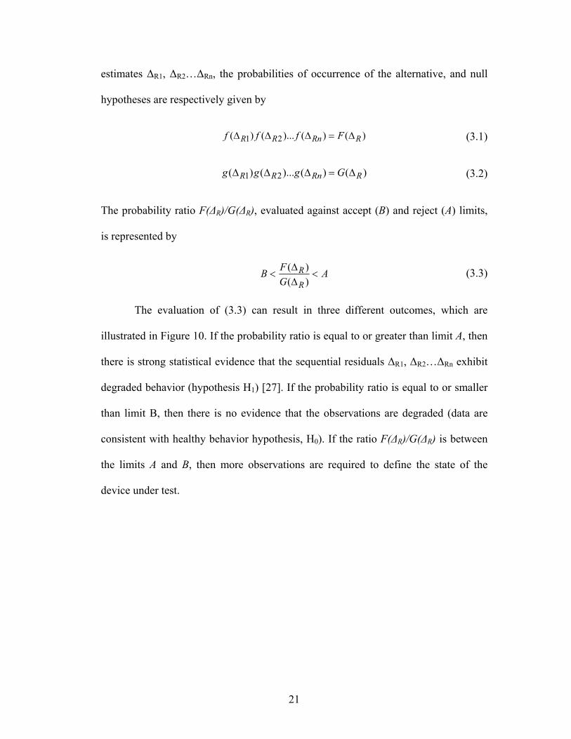
The evaluation of (3.3) can result in three different outcomes, which are
illustrated in Figure 10. If the probability ratio is equal to or greater than limit A, then
there is strong statistical evidence that the sequential residuals ΔR1, ΔR2…ΔRn exhibit
degraded behavior (hypothesis H1) [27]. If the probability ratio is equal to or smaller
than limit B, then there is no evidence that the observations are degraded (data are
consistent with healthy behavior hypothesis, H0). If the ratio F(ΔR)/G(ΔR) is between
the limits A and B, then more observations are required to define the state of the
device under test.
21

Figure 10. Potential outcomes in the evaluation of the probability ratio
The limits A, and B are respectively defined as functions of the false alarm,
and missed alarm probabilities and . Therefore, in the evaluation of a null, and
alternative hypothesis, it is possible to have either of four outcomes:
Reject H0 when H0 is true, with probability Known as type I error).
Reject H0 when H1 is true, with probability 1-(correct decision).
Accept H0 when H1 is true, with probability (Known as type II error).
Accept H0 when H0 is true, with probability 1-(correct decision).
With these considerations, the limits A, and B are defined as
22
1
A
(3.4)
1
B (3.5)
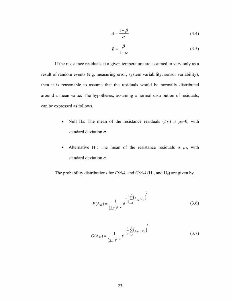
If the resistance residuals at a given temperature are assumed to vary only as a
result of random events (e.g. measuring error, system variability, sensor variability),
then it is reasonable to assume that the residuals would be normally distributed
around a mean value. The hypotheses, assuming a normal distribution of residuals,
can be expressed as follows.
Null H0: The mean of the resistance residuals (ΔRi) is μ0=0, with
standard deviation σ.
Alternative H1: The mean of the resistance residuals is μ1, with
standard deviation σ.
The probability distributions for F(ΔR), and G(ΔR) (H1, and H0) are given by
2
11
2
1
2/2
1)(
n
iRi
neRF
(3.6)
2
10
2
1
2/2
1)(
n
iRi
neRG
(3.7)
23

Inserting (3.4), (3.5), (3.6), and (3.7) into (3.3), setting μ0=0, and simplifying
the inequality, resulted in test criteria (SPRT index) for the resistance measurements:
1
1i 221Ln
nLn Ri
11 (3.8)
where μ is the mean defined by alternative Hypothesis, σ is the standard deviation for
H0 and H1, and ΔRi is the sequential residual i.
3.2 Methodology
The M-SPRT methodology consists of five steps: resistance characterization,
physics of failure model selection, model validation, SPRT definition and training,
and resistance monitor. The methodology is illustrated in Figure 11.
24

25
Figure 11. The M-SPRT methodology for monitoring contact resistance of electrical
interconnects

3.2.1 Resistance Characterization
When the methodology is considered for a reliability application, the
characterization may be performed using daisy chain packages, and a test assembly.
When the methodology is considered for a health monitoring application, the
characterization may be performed with a system assembly, and canary devices.
The resistance behavior of the electrical interconnect (contact) is analyzed as a
function of temperature (T). Resistance measurements are performed starting at 25 ºC
(room temperature), and in 10 °C increments, up to the maximum expected
temperature of the contact during the evaluation. As an alternative, the maximum
recommended operating temperature of the contact (as indicated in the specification)
can be used as the upper limit in the characterization test. For each test condition, the
resistance is measured when the assembly and contacts reach the target temperature.
The resistance characterization provides the expected (healthy) behavior of the
contact as a function of temperature.
3.2.2 Physics of Failure Model Selection
The contact design, materials, mechanical load assembly, environmental
conditions, and fundamental contact theory are analyzed to explain the resistance
behavior that was observed during the characterization experiment. A PoF model is
selected to estimate the contact resistance as a function of the stress environment.
Parameters for the model are extracted from the characterization data using regression
analysis. Finally, the PoF model is tested against the characterization data, and the
measuring error levels are verified to be within an acceptable range (e.g. estimate
error <0.5 mΩ).
26

3.2.3 Model Validation
The model validation is performed with the test assembly that was used during
the resistance characterization. For a reliability application, the assembly is subjected
to stress levels that are representative of the intended test environment. For health
monitoring applications, the assembly is subjected to nominal operating conditions.
The temperature (Ti) and resistance (Ri) are monitored continuously, identifying the
maximum temperature, and maximum resistance (Rm) of each test cycle/period. When
the experiment is completed, maximum resistance estimates (Re) are generated for
each one of the maximum temperatures using the PoF model. The estimates are
compared to the measurements, and the model is calibrated accordingly. This model
calibration is repeated until the resistance residual (the difference between estimated
and monitored maximum resistance) is acceptable (e.g. ΔR<1mΩ).
3.2.4 SPRT Definition and Training
The SPRT definition and training are performed with measurements that are
representative of the test or system environment. The measurements are performed
until a sufficient number of test cycles or hours are accumulated, enough to provide a
complete view of the application environment (either accelerated test, or health
monitoring). During the training period, the maximum temperature, and the resistance
of each test cycle or operating period are obtained from measurements (Ti, Ri); and a
resistance estimate (Re), and residual (ΔR) are calculated. The resulting array of
residuals is used to calculate the mean, and standard deviation of the null hypothesis
(H0). If the model is accurate, and if the maximum test conditions are consistent
during the training period, the mean of the residuals would be found to be zero (for a
27

normal distribution assumption). The mean μ1 of the alternative hypothesis (H1) is
selected considering the null hypothesis mean, and standard deviation (e.g. μ1 = μ0 +
3σ, σ1= σ0). Finally, the false alarm, and missed alarm probabilities (α, β) are selected,
and the SPRT index of (3.8) is defined.
3.2.5 Resistance Monitor
The resistance and temperature of the test samples are continuously monitored
for the duration of the experiment (the test duration for a reliability evaluation, or the
product life for a health monitoring application). The maximum contact resistance
and temperature values are extracted for each test cycle or period, the expected
resistances are calculated with the PoF model, and the resistance residuals are tested
with the SPRT. If any residual is found to be statistically different than that expected
by the null hypothesis, then the maximum contact resistance is considered degraded,
and an alarm is raised. If the residual is not found to be different, then the maximum
contact resistance is considered “healthy.” After either case, the monitoring process
continues. If during the evaluation the resistance measurements are found to decrease
over time, then the model validation, and the SPRT definition and training are
repeated, setting new values for the null and alternative hypotheses, and updating the
SPRT index (3.8). This retraining improves the test sensitivity by considering
situations where the contact resistance improves after initial assembly. The resistance
monitor process for a reliability application (temperature cycle test) is illustrated in
Figure 12.
28

Figure 12. Process for the monitoring and analysis of contact resistance data during a temperature cycle test. Rm is the maximum resistance during a test cycle
3.3 Experimental Demonstration
The M-SPRT methodology was demonstrated for a reliability evaluation,
using daisy chain packages as test vehicles, and a temperature cycle test as the stress
environment. The implementation of the methodology for health monitoring
applications would follow the same approach, but measuring canary devices during
typical system operation.
3.3.1 Experimental Setup
The IC socket utilized for the experiment is a 37 x 37 full array of Ag-filled
elastomer contacts. The contacts are molded into a Kapton film carrier, and protected
by a thermoplastic housing. The test assembly, which provided mechanical load and
access for resistance monitoring, consisted of a heatsink, daisy package, test board,
bolster plate, insulating Mylar, TIM, springs, screws, and IC socket [9]. When under
29

mechanical load, the IC socket and test assembly create the circuit illustrated in
Figure 13. To monitor the socket resistance during the experiment, a Keithley 7001
switch, and 580 microOhm meter were used.
Figure 13. Illustration of the daisy chain created by the test assembly and elastomer socket under compression. The interconnect matrix created by the Ag particles in the
elastomer are represented by the resistive network inside the two contacts
As shown in Figure 13, the total resistance consisted of circuit resistance (test
board + daisy chain), bulk contact resistance (two contacts in series), and contact to
pad resistances. Contact to pad resistance (Au to Ag) is very small in relation to bulk
and circuit resistances, so was ignored. The circuit resistance was found to be on
average 16.7 mΩ. The resistance of an individual elastomer contact, from test
assembly measurements, was estimated by
2
7.16 tR
iR (3.9)
30

where Rt is the total circuit resistance (board and package resistance, plus 2 contacts
in series). The measuring system error for the test setup was measured, and found to
be <0.05 mΩ.
3.3.2 Resistance Characterization
The resistance behavior of ten daisy chains was evaluated at six temperature
conditions: 25, 35, 45, 55, 65, and 75 °C. For each condition, the test assemblies were
allowed to dwell from 30 to 60 minutes, until the temperature and resistance
measurements were stable. For each temperature setting, the resistance of individual
contacts was estimated with (3.9), then recorded, finding resistance mean values of
4.8 mΩ at 25 °C, and 7.5 mΩ at 75 °C, as shown in Table 2.
Table 2. Resistance values from characterization test
Temperature (°C)
Mean (mΩ)
25 4.8 35 5.4 45 5.9 55 6.5 65 7.0 75 7.5
3.3.3 Physics of Failure Model Selection
The increase in elastomer contact resistance as a function of temperature
resulted from the interaction between the Ag particles and the elastomer. As the
temperature was increased, the elastomer expanded, disrupting the Ag-Ag contact
matrix inside the elastomer. The thermal expansion decreased the effective a-spot
31

area of the contact, and increased the overall resistance [28]-[35]. The contact
resistance, as a function of the effective a-spot radius, resistivity of Ag, and applied
temperature, can be described by [15], [36]
aeR T
2
(3.10)
0038.0*)15.293(*2020 TT (3.11)
where the constant 0.0038 is the thermal coefficient of resistivity for Ag.
Values of resistivity (T), and a-spot radius (a) were estimated for each test
sample and temperature, using the monitored resistance, and (3.10) and (3.11). A
power law used to model the effective a-spot radius behavior as a function of
temperature is [37]
mCTa (3.12)
Equation (3.12) can alternately be expressed as the linear equation
(3.13) bmxy
where y is ln(a), m is the slope, x is ln(T), and b is intercept, equal to ln(C). For each
test sample, the corresponding values of ln(a) and ln(T) were plotted, estimating the
coefficients with a linear regression analysis, as shown in Table 3. The model for the
effective a-spot radius of a contact at a given temperature was defined as
bmTa e (3.14)
32

Table 3. PoF parameters for test samples
Sample m b
1 -1.65 16.93 2 -1.73 17.33 3 -1.91 18.38 4 -1.78 17.67 5 -1.97 18.72 6 -2.09 19.43 7 -1.67 16.89 8 -1.81 17.74 9 -1.89 18.11 10 -1.99 18.71
3.3.4 Model Validation
The reliability evaluation used to demonstrate the methodology consisted of a
0/110 ºC temperature cycle test, having 20 minute dwell times at each extreme, and 8
minutes of ramp time. The daisy chain resistances, as illustrated in Figure 13, were
continuously monitored every 20 seconds.
From a pragmatic point of view, it was not possible to directly monitor the
temperature of each IC socket contact during the experiment. Therefore, a single
thermocouple was installed on the test board, one inch away from the contacts. An
important consideration for temperature cycle evaluations is that the temperature of
an IC socket contact lags behind that of the test board and the test chamber, a result of
thermal gradients, and thermal mass effects. To accurately estimate the maximum
resistance, it is necessary to quantify the difference between the contact and sensor at
the peak of the temperature cycle. The temperature gradient (ΔT), between the
elastomer contacts and the thermocouple, was estimated using the PoF model (3.14),
33

and the maximum contact resistance during a temperature cycle. For each maximum
contact resistance (Rm), an expected temperature value was obtained, resulting in the
temperature gradients shown in Table 4.
Table 4. Average temperature gradients for contacts at the maximum cyclic temperature
Sample ΔT
1 9.2 2 8.7 3 8.8 4 9.2 5 7.5 6 8.6 7 7.8 8 8.4 9 8.3 10 9.1
On average, the maximum contact temperature was found to be 9 °C below
that of the thermocouple. An updated PoF model, which incorporates the thermal
gradient between the thermocouple location (at temperature Tm) and the contact (at
temperature T’), is given by
'2''
aeR T (3.15)
where ρT’ is resistivity (estimated with maximum contact temperature T’), and a’ is
the effective a-spot radius at temperature T’.
Following the quantification of the thermal gradients, the temperature cycle
test was started, and contact resistance values were continuously monitored. The
cyclic resistance of all samples was found to decrease during the first 70 test cycles,
stabilizing after 100 cycles. Previous experiments on this contact technology have
34
also shown similar contact resistance decreases as a function of time and temperature
[38]. Therefore, the PoF model validation, and the definition and training of the SPRT
were performed using test data from test cycles 100 to 124 (monitor cycles 0 to 24).
For each test cycle, the maximum temperature was measured; using the
updated PoF model (3.15), a maximum resistance (Re’) was estimated. For all 25
validation cycles, the resistance estimates were found to be within 0.05mΩ from the
maximum contact resistance.
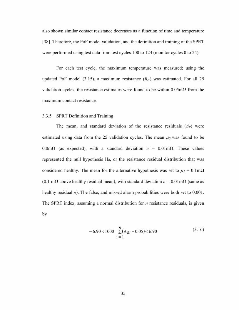
3.3.5 SPRT Definition and Training
The mean, and standard deviation of the resistance residuals (ΔR) were
estimated using data from the 25 validation cycles. The mean 0 was found to be
0.0mΩ (as expected), with a standard deviation σ = 0.01mΩ. These values
represented the null hypothesis H0, or the resistance residual distribution that was
considered healthy. The mean for the alternative hypothesis was set to 1 = 0.1mΩ
(0.1 mΩ above healthy residual mean), with standard deviation σ = 0.01mΩ (same as
healthy residual σ). The false, and missed alarm probabilities were both set to 0.001.
The SPRT index, assuming a normal distribution for n resistance residuals, is given
by
90.61i
05.0100090.6
n
Ri(3.16)
35

3.3.6 Resistance Monitor
The test board temperature and resistance of ten samples were continuously
monitored for 500 temperature cycles, after the resistance values were stable (monitor
cycles 0 to 500). For each cycle, the maximum contact temperature and resistance of
each sample were identified, a maximum resistance was estimated with the model
(3.15), and a resistance residual (ΔRi) was evaluated with the SPRT index (3.16).
Table 5 illustrates the monitoring results for one representative contact. After
114 monitor cycles, the resistance residual was considered “healthy,” having values
consistent with the null hypothesis [follows G(ΔR) in Figure 10]. During monitor
cycles 115-117, the residual status changed to “Unknown,” having values between
limits “A” and “B” of Figure 10. In monitor cycle 118, the resistance residual (ΔR118)
was found to be “Degraded” (follows F(ΔR) in Figure 10). After 119 monitor cycles,
the residual was considered “Healthy” again. The SPRT continued to produce
intermittent alarms in this fashion until monitor cycle 156, when the alarms became
continuous (a continuous alarm was defined as 5 or more continuous measurements
that exceed the SPRT limit). As shown in Table 5, the M-SPRT methodology was
capable of producing very accurate resistance estimates, and of detecting small
changes in resistance behavior. Given that the PoF model considered the effects of
temperature on the contact resistance, the accuracy of the estimates was not
compromised either by thermal variability or by measuring error of the test setup.
36

Table 5. Resistance monitor results of sample 5
Monitor Cycle
Tm (ºC) Rm
(mΩ)
Re
(mΩ)
CONTACT
STATUS PER
SPRT 26 96.1 7.79 7.77 Healthy 27 96.2 7.78 7.77 Healthy 28 96.1 7.78 7.77 Healthy ~ ~ ~ ~ ~
114 96.1 7.81 7.77 Healthy 115 96.0 7.81 7.77 Unknown 116 96.1 7.82 7.77 Unknown 117 96.0 7.81 7.76 Unknown 118 96.0 7.82 7.77 Degraded 119 96.1 7.81 7.77 Healthy 120 96.1 7.82 7.77 Unknown
* The digits for contact resistance are displayed for technique illustration purposes, showing the subtle and consistent shift in resistance that was observed in the experiment
Table 6 summarizes the results of the SPRT for all test samples. Six contacts
were found to decrease their resistance during the experiment, requiring new model
validation, and retraining of the SPRT. A new set of training measurements were
acquired, model parameters were estimated, and new SPRT index equations were
defined, just as illustrated by the loop to step 3 in Figure 11. The remaining four
samples were found to have s-significant increases in resistance, which were
consistent with the alternative hypothesis. In all cases, the increases in resistance were
detected in less than 120 cycles.
37

Table 6. Contact resistance monitor results for temperature cycle test
Sample Resistance
Status
Cycle to 1st Alarm
Cycle to Continuous
Alarm* 1 Decreased -- -- 2 Decreased -- -- 3 Decreased -- -- 4 Decreased -- -- 5 Increased 118 156 6 Increased 58 82 7 Increased 46 52 8 Increased 63 74 9 Decreased -- -- 10 Decreased -- --
* A continuous alarm is declared when 5 or more continuous measurements exceed SPRT limit
3.4 Conclusions
A PoF-SPRT methodology was presented for the modeling and monitoring of
resistance in electrical interconnects. The methodology, applicable for reliability and
health monitoring applications, was demonstrated for an accelerated test using an IC
socket assembly.
The resistance behavior of an IC socket contact was characterized at multiple
temperatures. The contact resistance was found to increase as a function of
temperature, from 4.8 mΩ at 25°C to 7.5 mΩ at 75°C. Contact characterization data is
important for reliability, health monitoring, and electronic prognostic applications
because it describes the “healthy” behavior of the electrical interconnect, and enables
the selection and definition of physics of failure models.
38

A physics of failure model, based on the effective a-spot radius, and the
resistivity of Ag, was developed for the elastomer socket. In addition, a power law
model was developed to represent the behavior of the a-spot radius. The PoF model
was used to provide resistance estimates as a function of temperature, and was shown
to be highly accurate. This modeling approach is very useful for reliability and health
monitoring applications because it produces low estimate errors, and because it takes
into consideration the changes in contact resistance that result from thermal
variability.
A SPRT was used to analyze the residuals (ΔRi) between the maximum
resistance measurements (Rm), and the PoF model estimates (Re). The M-SPRT
approach provides high sensitivity for the detection of resistance degradation events,
while allowing the selection of false and missed alarm probabilities. These
advantages are not provided by traditional threshold-based methods. This
methodology can be used to reduce test time requirements in reliability evaluations,
and to provide early detection of precursors of failure in health monitoring, and
electronic prognostic applications.
39

Chapter 4: Assessing the Reliability of Elastomer Sockets in Temperature Environments
4.0 Introduction
Land Grid Array (LGA) sockets are used in enterprise servers to interconnect
integrated circuits (ICs) with printed circuit board (PCB) assemblies. These
components offer an upgradeable, repairable, high density, and low cost alternative to
solder joints [4], [6].
The current common LGA sockets consist of an array of contacts in a polymer
housing that is compressed between the IC and the PCB. Three typical socket-contact
technologies are stamped metal, fuzz button, and elastomer. Elastomer contacts in
particular are composite structures where a carrier (elastomer) is filled with metal
particles (Ag). The shape and density of these filler particles are designed to optimize
mechanical and electrical properties. Elastomer contact technology is similar to
conductive adhesive joints, with the difference that it provides a separable
interconnection [30]-[34], [39].
In operation, mechanical loads are applied to IC sockets to compress the
contacts between metal pads and to create microscopic contact areas called a-spots.
When elastomer sockets are compressed, the contact expands perpendicular to the
applied force, creating multiple Ag-Ag particle contacts. As the mechanical load
increases, so does the effective a-spot area (the true contact area), with a resulting
decrease in interconnect resistance [15], [40].
40

The mechanical and electrical characteristics of elastomer sockets have been
discussed extensively in literature. Liu et al. [41] studied the effects of thermal and
mechanical stresses on the contacts (10-100 g, -55 to 150 °C), finding that resistance
behavior is strongly dependent on temperature and load.
Yang et al. [42] analyzed creep and stress relaxation failure mechanisms (with
force and deformation-controlled assemblies), using socket coupons and an automatic
contact-resistance probe. Creep, or time-dependent deformation, was found to reach
20-37% for temperatures between 40 °C and 150 °C (60-min exposure). Stress
relaxation, or load loss over time, reached 30%-40% for temperatures between 40 °C
and 125 ºC (100-min exposure). Contact resistance was estimated using a time-
dependent stress relaxation model, material hardness, and resistivity.
Yang et al. [7] performed electrical bias experiments to assess electro-
chemical migration (ECM). Highly accelerated stress test and 85°C/85% relative
humidity (RH) experiments were performed. Silver ECM was produced with 5 V
bias, causing a decrease in surface insulation resistance, from 109 to less than 105Ω
after 60 min of exposure.
Xie et al. [43] researched stiffness and stress relaxation behavior of contact
coupons under mechanical load and over temperature (10-100 g, 26 °C-183 ºC).
Temperature increases were found to decrease stiffness by 50% and to increase the
contact force relaxation by 50% after 1 h at 133 ºC.
Xie et al. [20] assessed the operating reliability of a 787 contact socket,
performing resistance measurements at multiple mechanical load settings. Test results
41

were fitted to an inverse Gaussian distribution, with the socket reliability for a 20 mΩ
resistance requirement estimated at 99.3%.
Lie et al. [21] researched reliability issues such as high temperature
dependence of resistance, high coefficient of thermal expansion, force deflection,
stress relaxation, deformation, and adhesion. They suggested that under some
conditions, elastomer contacts can exhibit electrical opens and shorts and intermittent
behavior during operation.
Liu [44] investigated the effects of moisture and corrosive gas exposure on
contact resistance. Elastomer sockets were found to be very resistant to moisture
attack (140 ºC/85%RH), having no swelling and no significant increase in resistance
after 150 h test. A mixed flowing gas environment (MFG class II) did not result in
detectable increases of resistance.
Previously, the operating temperature and RH environment for IC sockets in
an enterprise server application was quantified [19], and a temperature-dependent
physics-of-failure (PoF) model for the contact resistance was developed [12].
The reliability of elastomer sockets during the first year of life after assembly
has not been discussed in the literature, with most studies concentrating on contact
behavior over short periods of time. This paper investigates the reliability of
elastomer sockets in temperature conditions that are representative of postassembly
storage, enterprise server operation, and mild accelerated testing. The paper also
discusses the resistance behavior as a function of time and temperature, and the
assessment of contact reliability with a PoF model and a log-normal distribution.
42

4.1 Contact Resistance Distribution
The resistance of electrical contacts is fitted to statistical distributions to
estimate the probability that a given resistance value will be exceeded. Distribution
functions typically used to model contact resistance behavior are the normal, log-
normal, and inverse Gaussian, with normal distribution being applicable when
symmetric behavior exists [20]. The cumulative density function, in terms of
electrical contacts, provides the probability that a given resistance value will be
observed in a series of measurements. To assess the goodness-of-fit of these
distributions to experimental contact resistance data, a Kolmogorov-Smirnov test was
used.
4.2 Experimental Setup
4.2.1 Hardware
IC sockets require load assemblies in order to provide low and uniform
resistance connections between the LGA package and PCB pads. The experimental
assembly consisted of a heat sink, screws, springs, thermal interface material, ceramic
LGA package, IC socket, PCB, insulating Mylar film, and bolster plate [9], as shown
in Figure 14. A study of the assembly component dimensions and spring constants
estimated the applied load to be at 78 g per contact (see Appendix II). Shadow Moiré
analysis of the LGA packages and bolster plates confirmed that the load-bearing
surfaces met assembly flatness specification, a requirement needed to ensure load
uniformity across all socket contacts (see Appendix III).
43

Figure 14. Illustration of the load assembly components used for the experiment.
The socket is compressed between the LGA package and PCB pads
Tyco 1.0 elastomer sockets were used to interconnect ceramic daisy chain
packages with PCBs. The socket is a 37 x 37 array of Ag-filled elastomer contacts,
molded into a Kapton polyimide film and a thermoplastic housing, as shown in Figure
15. The daisy chain package and test-board assembly enable four-wire resistance
measurements for 22 short chains, each one with two contacts in series, as shown in
Figure 16.
44

Figure 15. Illustration of an elastomer socket showing the 37 x 37 array of contacts, Kapton film (dark regions between contacts), and thermoplastic housing (perimeter)
Daisy Chain Package
Test Board
ElastomerContacts
4-wireHigh
Source
Sense
4-wireLow
Source
Sense
rd
rC2
rT1
rT2
rC1
Figure 16. Illustration of a two-contact chain formed by the test assembly and the
IC socket. Four-wire method is used for resistance measurements. rc1 and rc2 are the contact bulk resistance. rT1 and rT2 are the test board circuit resistance. rd is the
package resistance. The resistance network inside contacts represents that of Ag-Ag particle contacts
45
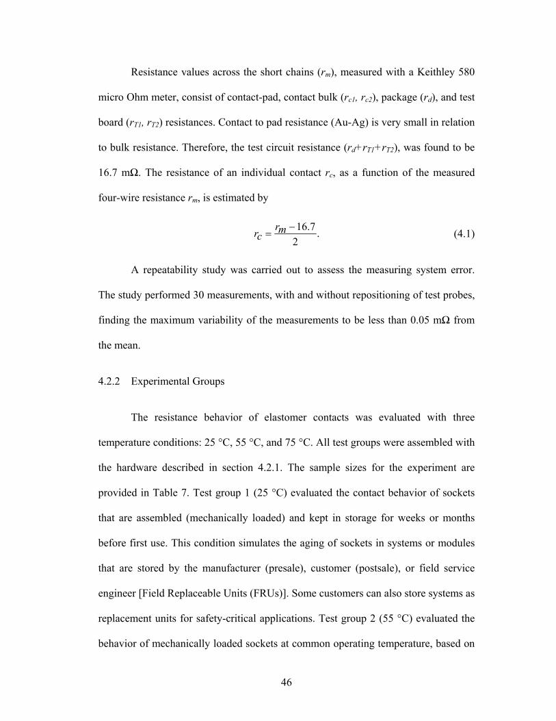
Resistance values across the short chains (rm), measured with a Keithley 580
micro Ohm meter, consist of contact-pad, contact bulk (rc1, rc2), package (rd), and test
board (rT1, rT2) resistances. Contact to pad resistance (Au-Ag) is very small in relation
to bulk resistance. Therefore, the test circuit resistance (rd+rT1+rT2), was found to be
16.7 mΩ. The resistance of an individual contact rc, as a function of the measured
four-wire resistance rm, is estimated by
.2
7.16 mr
cr (4.1)
A repeatability study was carried out to assess the measuring system error.
The study performed 30 measurements, with and without repositioning of test probes,
finding the maximum variability of the measurements to be less than 0.05 mΩ from
the mean.
4.2.2 Experimental Groups
The resistance behavior of elastomer contacts was evaluated with three
temperature conditions: 25 °C, 55 °C, and 75 °C. All test groups were assembled with
the hardware described in section 4.2.1. The sample sizes for the experiment are
provided in Table 7. Test group 1 (25 °C) evaluated the contact behavior of sockets
that are assembled (mechanically loaded) and kept in storage for weeks or months
before first use. This condition simulates the aging of sockets in systems or modules
that are stored by the manufacturer (presale), customer (postsale), or field service
engineer [Field Replaceable Units (FRUs)]. Some customers can also store systems as
replacement units for safety-critical applications. Test group 2 (55 °C) evaluated the
behavior of mechanically loaded sockets at common operating temperature, based on
46

previous studies of enterprise server applications [19]. This condition allows the study
of thermal effects on contacts during operation, without the influence of electrical
bias. Test group 3 (75 °C) evaluated sockets at an accelerated load condition. The
temperature was chosen to reduce overacceleration effects which can introduce
mechanisms or behavior not relevant for nominal operating conditions. This
consideration was important due to the documented complex behavior of the
elastomer socket [7], [20], [21], [41]-[43].
Table 7. Sample sizes for experimental test groups
Group TemperatureTest
Boards Daisy Chains
1 25 ºC 7 154 2 55 ºC 7 154 3 75 ºC 4 88
4.2.3 Test Procedure
Samples from group 1 were assembled, the resistance measured, and stored in
an office environment (~25 °C). Samples from groups 2 and 3 were assembled,
measured, and placed inside temperature chambers at 55 ºC and 75 °C, respectively.
At predetermined time intervals the samples, from all test groups were taken out of
their test conditions, allowed to dwell at room temperature for 1 h, measured, and
returned to their respective test environment.
All groups were tested for 2000 h. Selected samples from groups 1 and 3 were
further tested to provide insight into the contact behavior during the first year of life.
Group 1 samples (88 contacts) were tested up to 16 500 h. Group 3 samples (88
47

contacts) were tested up to 4500 h. Group 2 samples were not tested beyond 2000
hours.
4.3 Results and Discussion
4.3.1 Resistance Behavior
The contact resistance measurements from the three test groups were fitted to
normal, log-normal, and inverse Gaussian distributions. None of the assumed
statistical distributions provided an acceptable fit for the 25 °C data, which exhibited
nonlinear behavior on probability plots. Fitting to other statistical distributions, such
as Weibull, was also unsuccessful. A closer examination of the data showed that the
observations were the result of a mixed population and having two modes and a
mixed/transition period. An excellent fit was obtained using a three-population
mixed-Weibull distribution model, as shown in Figure 17.
48

Contact Resistance (mOhm)
Res
ista
nce
CDF
(%)
1.0 20.010.00.1
0.5
1.0
5.0
10.0
50.0
90.0
99.9
0.1
T0T500T1000
T16500T2000
Population 1
Population 3
Population 2
T0T16500
Figure 17. Three-population mixed-Weibull probability plot for resistance of elastomer contacts evaluated with 25 ºC condition. Measurements and fit lines for 0,
500, 1000, 2000, and 16500 h are shown
Population 1 consists of the samples in the high slope portion of the curves.
Population 3 consists of the samples in the low slope portion of the curves.
Population 2 is the knee/transition region. Measurements at T0, T500, T1000, T2000,
and T16500 hours are shown. The average contact resistance for the samples in the 25
°C condition decreased 25% after 2000 h. Using the mixed-Weibull model, it was
estimated that, after 16500 h, approximately 40% of the samples (population 1) had a
Weibull slope β=14, and 20% (population 3) had a Weibull slope β=6.
In elastomer sockets under applied loads, there is significant amount of
viscoelastic deformation, which can result in stress relaxation if the structural
configuration constrains the deformations in any way. When an elastomer contact is
mechanically loaded, the elastomer portion of the matrix starts to creep, resulting in
49

contact radial expansion and height reduction. After the socket stops are reached
(which are provided to prevent overloading), the assembly is constrained from further
deformation and the stresses progressively relax in the elastomer. Furthermore, the
applied mechanical loads are transmitted by the elastomer matrix to the silver
particles distributed throughout the matrix. These Ag particles can then experience
physical contact with neighboring particles, creating microscopic contact regions
called a-spots. As the elastomer undergoes stress relaxation at an average macroscale,
the applied mechanical stresses can internally redistribute, resulting in increased
contact stresses at the microscale, between the Ag particles. This increasing contact
stress can lead to an increase of the effective contact area between the Ag particles,
particularly if the Ag undergoes any creep deformation at this temperature. The net
effect is a reduction in contact resistance over time, although the average stress in the
elastomer interconnect appears to decrease at the macroscale.
In the test assembly utilized for this experiment and with the 78 g load
applied, the elastomer creeps rapidly (within minutes) until the socket stops are
reached. Test results show that contact resistance decreases over time. Elastomer
stress relaxation, which causes an increase in contact resistance, is not a predominant
mechanism within this timeframe of the loading conditions. Cross-sectional analysis
of a socket assembly at the beginning of the experiment confirmed that the socket
stops had been reached. The observed reduction in resistance results from an increase
in the effective contact area between the Ag particles, either from an increase in area
of the existing Ag-Ag a-spots or from the creation of additional a-spots. Population 1
in Figure 17, exhibiting the greatest decrease in resistance over time, represents the
50

fraction of the elastomer contacts where an increase of the effective a-spot area is the
dominant mechanism. Population 3 in Figure 17, exhibiting higher resistance values
over time, represents the fraction of the contacts where elastomer relaxation is
becoming a more dominant mechanism. More studies are necessary to further
investigate this behavior.
The changes in statistical distribution exhibited by samples in the 25°C
condition (Figure 17) are of concern for the long-term reliability of the socket. As the
contact ages, this behavior could result in a rapid decrease of reliability over time,
particularly for units that have been assembled and stored for over a year.
The 55 °C data (up to 2000 h) exhibited linear behavior in the probability
plots and was fitted with a log-normal distribution, as illustrated in Figure 18. The
average contact resistance decreased 20% during the first 500 h and 35% after 2000
h. The shape parameter increased 30% in the same period, changing the distribution
shape from normal to log-normal. The 75 °C data displayed nonlinear resistance
behavior in a log-log plot, particularly after 500 test hours. A three-parameter Weibull
distribution was found to provide an acceptable fit to the data up to 2900 h, as
illustrated in Figure 19. For the 4500 h data, a mixed-Weibull model provided a better
fit. Notice in Figure 19 the changing distribution slope over time, which suggests a
degrading reliability. Overall, the mean contact resistance decreased 45% in the first
500 h and 50% after 2000 h. The added reduction in resistance in this test group,
when compared to that observed in the 25 ºC and 55 ºC groups can be explained by
the higher stress temperature, which induces lower stiffness (elastomer), higher
thermal expansion (elastomer, Ag, and assembly), and higher stresses (between Ag
51

particles). The change of distribution to a mixed-Weibull model at 4500 test hours
indicates a change in the dominant mechanism, from a Ag particle-related
mechanism, to elastomer stress relaxation.
Contact Resistance (mOhm)
Res
ista
nce
CDF
(%)
1.0 20.010.00.1
0.51.0
5.0
10.0
50.0
99.9
0.1
T0
T1000T2000
T500
T0T2000
Figure 18. Log-normal probability plot for elastomer contact resistance evaluated
with 55 ºC condition. Measurements and fit lines for 0, 500, 1000, 1500, and 2000 hare shown. The resistance behavior is linear in the logarithmic scale. Each data set
consists of 154 measurements
52

Contact Resistance (mOhm)
Res
ista
nce
CDF
(%)
1.0 20.010.00.1
0.5
1.0
5.0
10.0
50.0
90.0
99.9
0.1
T0
T4500
T1000T2000T2900
T500
T0
T4500
Figure 19. Three-Parameter Weibull probability plot (uncorrected for gamma) for elastomer contact resistance evaluated with 75 ºC condition. Measurements and fit
lines for 0, 500, 1000, 2000, 2900, and 4500 h are shown
Test results show that while the temperature used for test group 2 (55 °C) was
able to drive a consistent and stable contact aging, this is not the case for higher or
lower temperatures. Accelerated tests on this contact technology can produce
behavior and failures that are not present under nominal operating conditions. If the
temperature is too low or too high, the effect of Ag particles in the matrix can be
underestimated or overestimated. Therefore, over acceleration of elastomer contacts
can mask the true long term effects of elastomer stress relaxation.
While the resistance behavior is represented by multiple statistical
distributions, it is possible to model the mean contact resistance over time and
temperature. Mean resistance values for all test groups and times were calculated,
53

with results provided in Table 8. Values for extended test times (2900, 4500, 16 500
h) are also included.
Table 8. Mean contact resistance for test group data
μ (mΩ) μ (mΩ) μ (mΩ) Time
25 ºC 55 ºC 75 ºC 0 7.8 8.2 7.0
500 6.9 6.2 4.2 1000 6.5 5.5 3.9 1500 6.2 5.2 3.7 2000 6.0 5.1 3.7 2900
aT
2
*)15.293(*2020 TT
4.3.2 Time-Dependent Model for Mean Contact Resistance
The resistance of an elastomer contact is a function of the true contact area
(effective a-spot), the resistivity of silver, and the stress relaxation of the elastomer.
Since the elastomer relaxation is not a predominant mechanism for the temperature
conditions utilized in this experiment, the model will be defined only as a function of
the contact area and resistivity of Ag. A model to describe the mean contact
resistance is [42]
(4.2)
(4.3)
where μ is contact resistance (Ω), ρT is resistivity of Ag as a function of temperature,
a is effective a-spot radius (true contact area radius), ρ20 is resistivity of Ag at 20 °C,
3.5 4500 3.5
16 500 5.2
54
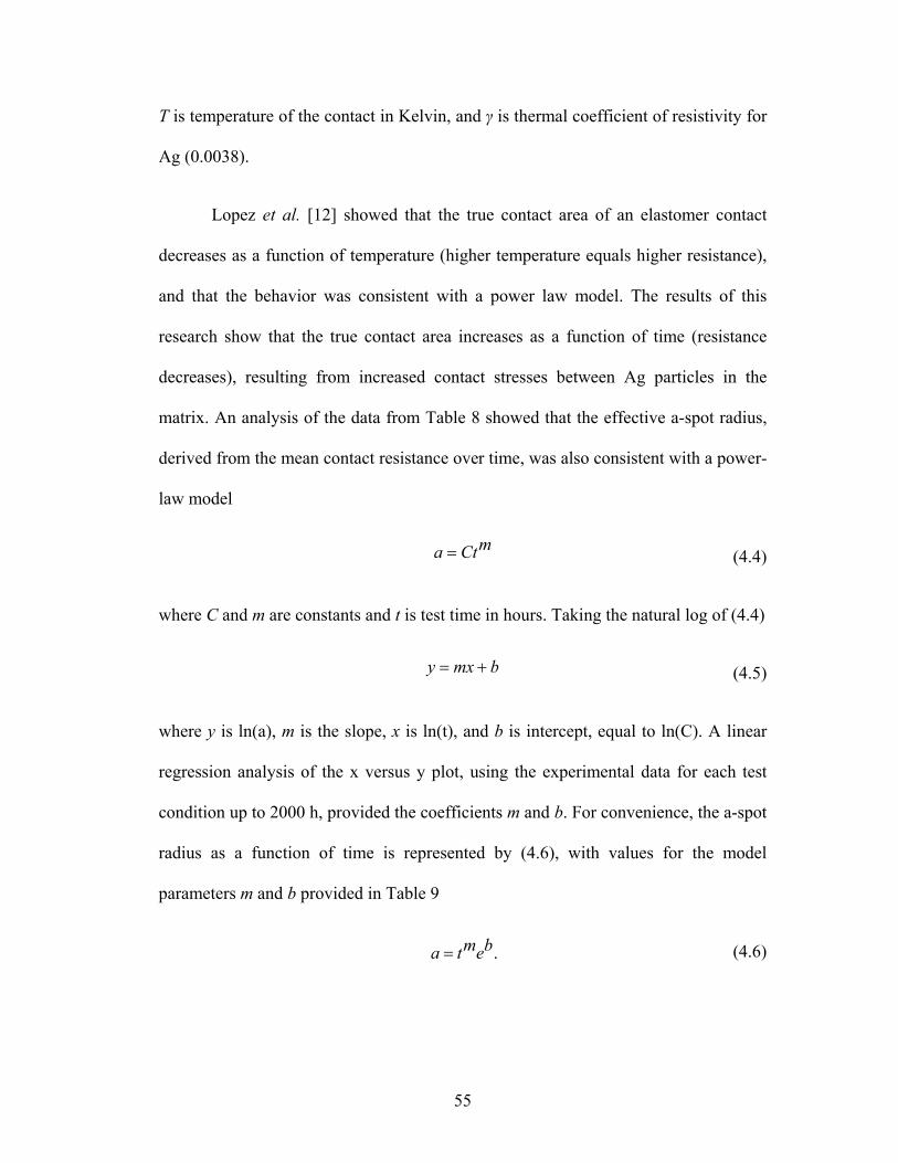
T is temperature of the contact in Kelvin, and γ is thermal coefficient of resistivity for
Ag (0.0038).
Lopez et al. [12] showed that the true contact area of an elastomer contact
decreases as a function of temperature (higher temperature equals higher resistance),
and that the behavior was consistent with a power law model. The results of this
research show that the true contact area increases as a function of time (resistance
decreases), resulting from increased contact stresses between Ag particles in the
matrix. An analysis of the data from Table 8 showed that the effective a-spot radius,
derived from the mean contact resistance over time, was also consistent with a power-
law model
mCta (4.4)
where C and m are constants and t is test time in hours. Taking the natural log of (4.4)
bmxy (4.5)
where y is ln(a), m is the slope, x is ln(t), and b is intercept, equal to ln(C). A linear
regression analysis of the x versus y plot, using the experimental data for each test
condition up to 2000 h, provided the coefficients m and b. For convenience, the a-spot
radius as a function of time is represented by (4.6), with values for the model
parameters m and b provided in Table 9
.bemta (4.6)
55

Table 9. Parameters for PoF model – three groups
Test Group
m b
1 0.085 -14.16 2 0.111 -14.18 3 0.097 -13.74
The model given by (4.2), (4.3), and (4.6) was used to estimate the mean
contact resistance of the elastomer socket and is plotted against experimental results
shown in Figure 20. For all test groups and test times, the model estimates were
within 3% of actual observations. Extended test results for groups 1 and 3, which
were not used to create the model, were also found to be within 3% of the estimates.
See Appendix VI for a generalized form of the model.
Figure 20. Plot for the mean contact-resistance model as a function of time for 25 ºC,
55 ºC, and 75 ºC conditions. The model estimates (fit lines) and experimental measurements (markers) are shown. Notice the model fit for extended test results at
75 ºC (2900 and 4500 h, lower curve) and 25 ºC (16 500 h, upper curve)
56

4.3.3 Contact Reliability
The contact resistance behavior at normal operating temperature can be
estimated with a log-normal – power-law relationship
e
r
rrf 2'2
')ln(
'2
1)(
2
(4.7)
where r is contact resistance, σ’ shape parameter, and μ’ the mean of the natural log
of resistance [estimated with (4.2), (4.3), and (4.6)]. The reliability of the elastomer
contact and socket were estimated assuming a resistance requirement of r ≤ 20 mΩ,
nonbias operation at 55 ºC, and a series reliability model [27]. For the first year of
operation, the reliability was determined to exceed 99.99% for both contact and
socket, as shown in Table 10.
Table 10. Estimated reliability for first year under nonbias conditions
Elapsed Time Log-normal
Shape* Parameter
Estimated Mean**
Resistance (mΩ)
Contact Reliability
Socket Reliability
(1369 contacts)
1 Month 0.202 5.59 >99.99% >99.99% 3 Months 0.226 4.93 >99.99% >99.99% 6 Months 0.235 4.56 >99.99% >99.99% 12 Months 0.240 4.22 >99.99% >99.99%
* Shape parameter values from test data. Six and twelve month parameters estimated from extended test results (16500 hours at 25 ºC and 4500 hours at 75 ºC).
** Mean resistance estimated with PoF model described in section 4.3.2
While the first year reliability is high, it was shown that the contact has
changes in the resistance distribution over time and temperature that are not desirable
for the long term reliability of the socket. As the contact ages and elastomer stress
57

relaxation becomes a dominant mechanism, the observed distribution changes will
reduce product reliability by increasing the probability of higher resistance values.
For the case of elastomer sockets that are assembled and stored at room temperature
before first use (as in backup systems, replacements in safety critical applications,
FRUs, and spare assemblies), the contacts will experience a significant increase in the
probability of failure after 2000 h.
Socket assemblies tested at 55 ºC condition display an increase in the
probability of failure as a result of steady increases in the log-normal shape
parameter, from 0.15 at the beginning of the test and up to 0.23 after 2000 h (seen as
decrease in slope over time in Figure 18). At 75 °C, there is also a decrease in slope
over time. The decrease in slope results in an increased probability of contact failure
over time, which is an important factor for high-density IC sockets (1500+ contacts)
and multisocket systems.
4.4 Conclusions and Recommendations
This paper investigated the resistance behavior of metal-filled elastomer
sockets that were mechanically loaded and subjected to non-bias temperature
conditions representative of postassembly storage, normal temperature operation, and
accelerated testing conditions. Contact resistance was shown to decrease as a function
of time and temperature after 2000 test h (25% at 25 ºC, 50% at 75 ºC). This decrease
in resistance should be considered in quality, reliability, and health-monitoring
applications to define baseline resistance characteristics and to improve failure
detection sensitivity.
58

The resistance of sockets evaluated at 25 ºC (postassembly) was found to
follow a mixed-population Weibull distribution. This condition was shown to be
undesirable for long-term socket reliability because it increased resistance variability
over time, which can result in unacceptable increases in the occurrence of failure. It is
recommended that elastomer socket assemblies, as the ones described in this study,
should not be stored for long periods of time (months) before first use.
The resistance of sockets evaluated at 55 ºC (common operating temperature)
showed linear behavior in the log-log scale, with a log-normal distribution providing
the best fit. The log-normal scale parameter was found to increase over time,
changing the distribution shape and gradually increasing probability of higher
resistance values. The resistance behavior of sockets evaluated at 75 ºC (accelerated
temperature) was best fitted by a three-parameter Weibull distribution. The
distribution parameters for this condition were also found to vary over time.
Changing parameters in the statistical distribution of resistance are important
reliability indicators. These parameters should be closely monitored in IC socket
evaluations to allow an understanding of trends and potential failures of the contact
technology.
The test results show that the contact resistance behavior of elastomer sockets
is defined by multiple statistical distributions over temperature and time. This
statistical variation is an indicator of multiple active mechanisms on the elastomer
contact. As a result, tests performed at conditions above or below the common
operating temperature (55 ºC) could mask the effect of failure mechanisms and lead
to erroneous conclusions. It is recommended that conditions used to evaluate
59
elastomer sockets are carefully reviewed to ensure that stress and stress levels are
accelerating the desired behavior.
A PoF model of the mean contact resistance was developed and combined
with a log-normal distribution to estimate the socket reliability. This is significant
because the model can be used to estimate the probability of failure of an elastomer
contact, socket, or sockets in a system, as a function of temperature and of contact
age, in which probability is a key parameter to estimate system reliability. The model
is suggested for first-level socket reliability estimates in enterprise servers.
Further experiments are required to study the effects of elastomer stress
relaxation in the contact behavior during the second and third year of operation at
common operating temperature. Other studies are also needed to assess the combined
effect of temperature and electrical bias on the long-term reliability of this contact
technology.
60

Chapter 5: Effects of Electrical Bias on Contact Resistance
5.0 Introduction
Electrical bias is a key element in the operating environment of IC sockets. In
typical applications roughly 45% of contacts perform power and ground functions,
while 55% perform signal and signal control functions. Understanding the effects of
electrical bias is therefore important for any contact reliability analysis.
The research presented in Chapter 4 studied the contact resistance behavior of
mechanically loaded contacts as a function of time and temperature. In this chapter
elastomer contacts, also under mechanical load, were stress tested with 200, 250, 300,
and 350 mA bias current, representative of nominal and accelerated operating
conditions. The experiment monitored changes in resistance as a function of electrical
bias and time.
5.1 Experimental Setup
As shown in Figures 17, 18, and 19 (Chapter 4), elastomer contacts under
mechanical load display greater resistance variability when they are maintained at
ambient temperature. Therefore, to maximize resistance degradation, and to minimize
the effect of temperature on the contact, a test condition of 25 ºC was selected. Seven
test boards with daisy chain packages (illustrated in Figure 13, Chapter 3) were wired
and connected to a ballast resistor and power supply, as shown in Figure 21.
61

+-
Rcontact
Rballast
Vs
Figure 21. Test circuit for bias experiment. The power supply and ballast resistor are set to provide the required current flow for each test cell. The dashed line represents
the thermal chamber (set to 25 °C)
From the daisy chain packages 16 samples were selected for electrical bias
testing and 43 for control purposes. The location of all control samples was selected
to be within 10mm from the bias samples, this to reduce the resistance variability that
results from package surface effects. The contact resistance was measured for all
samples at the beginning of the experiment and at predetermined intervals, up to 2000
hours. The test groups, sample sizes, and bias conditions are shown in Table 11.
Table 11. Test cells and sample sizes for electrical bias experiment
Cell Bias Current
(mA) Sample Size Comments
1 200 6 Nominal current 2 250 4 +25% current 3 300 4 +50% current 4 350 2 +75% current
Control --- 43 ---------------
62

5.2 Results and Discussion
The contact resistance measurements of the control samples were analyzed
and fitted to Log-normal and Weibull distributions. A three-Parameter Weibull model
was found to provide the best fit to the data, as illustrated in Figure 22. Notice that the
resistance behavior is not identical to the one shown in Figure 17 (Chapter 4), for the
25º C condition. This behavior difference is attributed to the smaller sample size used
in this experiment and to the selection of specific package locations for monitoring.
Contact Resistance (mOhm)
Res
ista
nce
CDF
(%)
1.0 10.01.0
5.0
10.0
50.0
90.0
99.9T0T2,000
Figure 22. Three-Parameter Weibull probability plot of control samples at 25 ºC condition. Measurements and fit lines for 0 and 2000 hours are shown
63
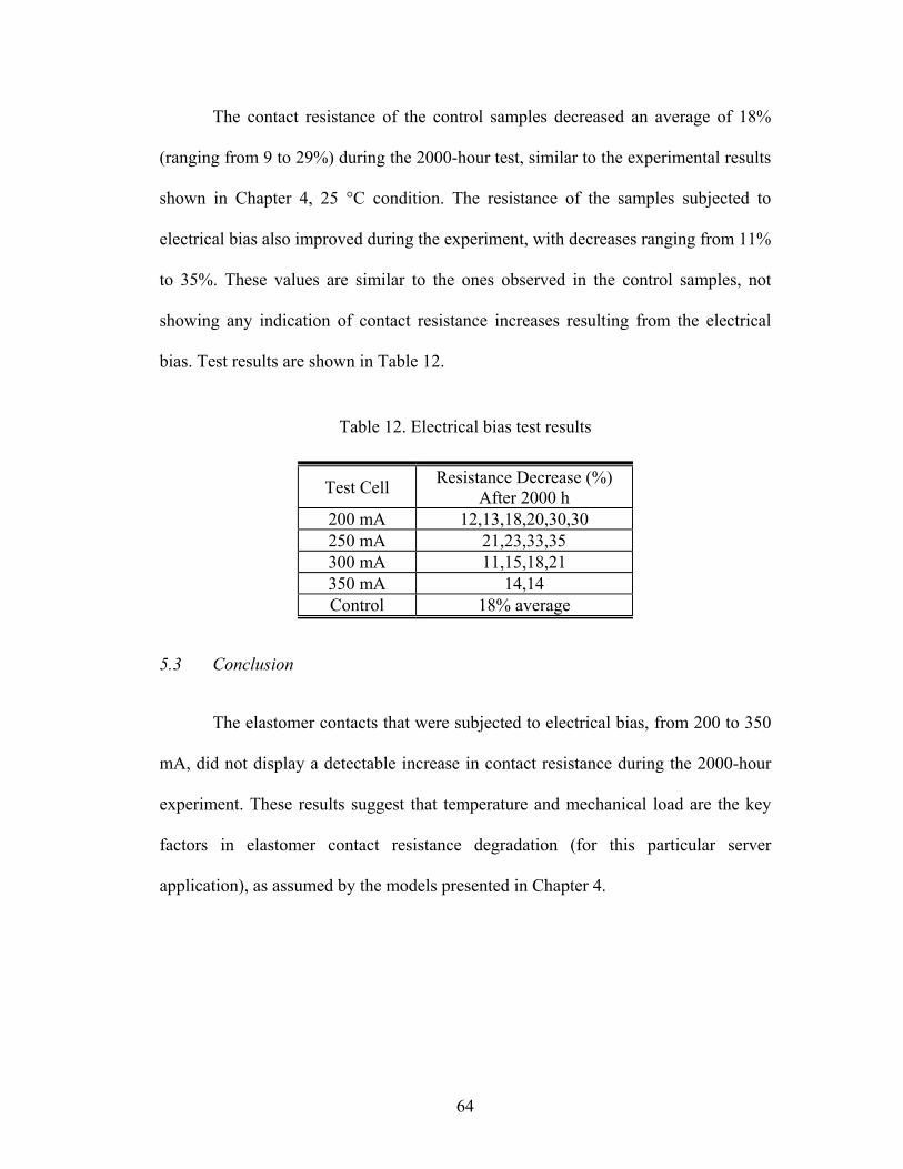
The contact resistance of the control samples decreased an average of 18%
(ranging from 9 to 29%) during the 2000-hour test, similar to the experimental results
shown in Chapter 4, 25 °C condition. The resistance of the samples subjected to
electrical bias also improved during the experiment, with decreases ranging from 11%
to 35%. These values are similar to the ones observed in the control samples, not
showing any indication of contact resistance increases resulting from the electrical
bias. Test results are shown in Table 12.
Table 12. Electrical bias test results
Test Cell Resistance Decrease (%)
After 2000 h 200 mA 12,13,18,20,30,30 250 mA 21,23,33,35 300 mA 11,15,18,21 350 mA 14,14 Control 18% average
5.3 Conclusion
The elastomer contacts that were subjected to electrical bias, from 200 to 350
mA, did not display a detectable increase in contact resistance during the 2000-hour
experiment. These results suggest that temperature and mechanical load are the key
factors in elastomer contact resistance degradation (for this particular server
application), as assumed by the models presented in Chapter 4.
64

Chapter 6: Sources of Failure in IC Socket Contacts
6.0 Introduction
To analyze the potential sources of failure for IC socket contacts it is
imperative that a “life cycle” point of view be considered. By examining the different
life phases it is possible to identify issues that result from the contact design, system
design, system components, system assembly, transportation, operating environment,
and socket-system interactions, among others. The sources of failure during the IC
socket life cycle are illustrated in Figure 23 and will be discussed in the following
sections.
6) System Service and
Repair
5) SystemOperation
4) SystemStorage and
Transportation
3) SystemAssembly
2)Manufacturing
1) Design
SocketFailures
6) System Service and
Repair
5) SystemOperation
4) SystemStorage and
Transportation
3) SystemAssembly
2)Manufacturing
1) Design
SocketFailures
Figure 23. Sources of failure for IC socket contacts
65

6.1 Design
Design is the key contributor of failures for IC socket technologies [52]-[54].
Some IC sockets, such as the CIN::APSE® [55], are known in industry for their
superior quality, reliability, and high cost. Other technologies, such as the metal-in-
elastomer, are known in industry for their excellent quality, lower reliability, and low
cost. For illustration purposes, the differences between these two socket technologies
will be briefly discussed.
The Cinch CIN::APSE® socket consists of an array of buttons that are carried
on a plastic housing. Each button is made of 7 bundled wires, that when compressed,
provide physically independent, point-to-point, current paths. The contact absorbs
100% of the applied load, does not wipe the IC and PCB pad surfaces, and maintains
its position during temperature excursions. An important feature of this design is that
not all wires in a contact are required for successful operation. This contact design
has embedded redundancy, which is used in high reliability systems. A SEM image of
a CIN::APSE® contact is shown in Figure 24. A reliability block diagram that can be
used to represent this contact technology is illustrated in Figure 25.
66

Figure 24. SEM SE (20KV, 300x) image of a Cinch CIN::APSE contact
R1
R2
R3
Rn
x/n
Figure 25. Reliability block diagram of an “x-out-of-n” system, representative of a
CIN::APSE contact. x represents the minimum number of wires needed for successful operation and n represents the total number of wires
The elastomer socket consists of an array of buttons that are molded on top of
a Kapton® film, and carried by a plastic housing. Each button is made of Ag-filled
elastomer, that when compressed, provides hundreds of interconnected current paths.
67

Because it is a composite structure, any load applied to an elastomer contact is shared
between the elastomer and the Ag particles. Just as CIN::APSE®, this contact
technology does not wipe the IC and PCB pad surfaces. An important difference is
that the elastomer contact does not maintain the position of the interconnected paths
during temperature excursions. As the contact is heated up, the elastomer experiences
radial expansion, and all Ag-Ag particle interfaces are gradually disrupted. This
contact design has an embedded coupling factor (elastomer), which can result in
lower socket reliability. A high magnification cross-sectional image of an elastomer
contact, showing the elastomer and Ag particles, is shown in Figure 26. A reliability
block diagram that can represent the elastomer contact is illustrated in Figure 27.
Figure 26. SEM BSE image (25KV, 1000x) of a Ag-filled elastomer contact cross section. The dark region on the middle-right is the Kapton carrier. The light colored
areas are Ag. The dark colored areas are elastomer
68

Rp
Rp
Rp
Rp
ComplexSystem
Re
Rp
Rp
Rp
Rp
Rp
Rp
Rp
Rp Rp
Figure 27. Reliability block diagram representing an elastomer contact. Re is the contact reliability due to the elastomer (coupling factor). Rp is the reliability of the
contact due to the Ag-Ag particle interactions
From the brief technology descriptions above it is easy to see that a contact
designed with embedded redundancy can be expected to have higher reliability than a
contact designed with embedded coupling factors. The presence of a root cause and a
coupling factor between components or systems is known in reliability literature as
common cause failures (CCF) [56], which are found in low reliability systems.
Contrasting the characteristics that exist or do not exist in a contact
technology can be an important tool for the identification of the sources of failure.
With these considerations in mind, a list of design factors that can induce IC socket
failures is shown in Table 13.
69
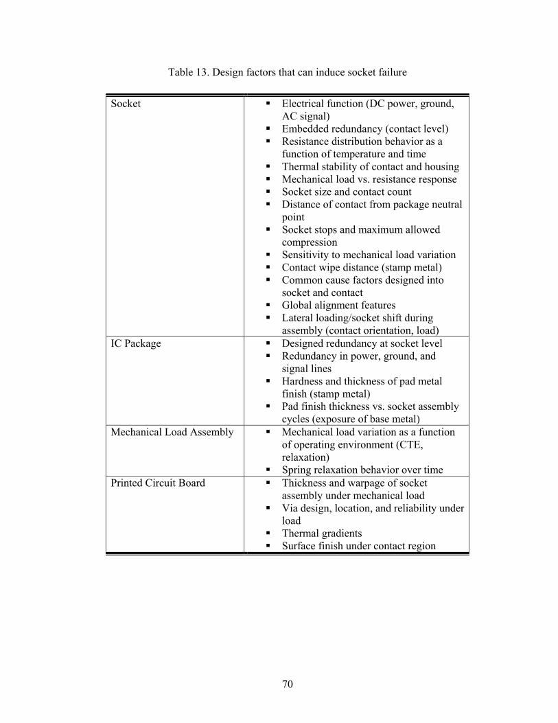
Table 13. Design factors that can induce socket failure
Socket Electrical function (DC power, ground, AC signal)
Embedded redundancy (contact level) Resistance distribution behavior as a
function of temperature and time Thermal stability of contact and housing Mechanical load vs. resistance response Socket size and contact count Distance of contact from package neutral
point Socket stops and maximum allowed
compression Sensitivity to mechanical load variation Contact wipe distance (stamp metal) Common cause factors designed into
socket and contact Global alignment features Lateral loading/socket shift during
assembly (contact orientation, load) IC Package Designed redundancy at socket level
Redundancy in power, ground, and signal lines
Hardness and thickness of pad metal finish (stamp metal)
Pad finish thickness vs. socket assembly cycles (exposure of base metal)
Mechanical Load Assembly Mechanical load variation as a function of operating environment (CTE, relaxation)
Spring relaxation behavior over time Printed Circuit Board Thickness and warpage of socket
assembly under mechanical load Via design, location, and reliability under
load Thermal gradients Surface finish under contact region
70

6.2 Manufacturing
Manufacturing defects or variability that can induce contact failures are
typically detected by outgoing and incoming inspections. Nevertheless, it is not
uncommon to have defects or out-of-specification material that escapes these
inspections and produces a decrease of quality and/or reliability. Besides the obvious
socket concerns it is important that LGA package, mechanical load assembly
components, PCB, storage, and transportation factors are considered and monitored
on a regular basis. These factors are provided in Table 14.
Table 14. Manufacturing factors that can induce socket failure
Socket Handling LCP flash Elastomer flash Knit lines, cracks, and crack propagation
pattern “Improvement” of manufacturing
process Changes of material or material supplier Changes of metal particle concentration
and shape (elastomer) Contamination (fiber, dust, oil) Manufacturing variability (dimension)
IC Package Surface flatness, shape, and variation Pad finish defects
Mechanical Load Assembly Defective or out of specification components
Component variability (excessive) Change of supplier Shape, flatness, and variation of bolster
plate Printed Circuit Board Contamination and/or factory residues Socket Storage and Transportation
Storage duration and environmental conditions
Exposure to corrosive gases
71

6.3 System Assembly
IC sockets are not independent or isolated components of a system, but rather
part of highly integrated assemblies. Failures can result from assembly specification
issues, operator mistakes, material damage, contamination, and socket/assembly
deformation after application of the mechanical load. These sources of failure are
shown in Table 15.
Table 15. System assembly factors that can induce socket failure
Socket Handling damage Contact residue on pad Dust Improper socket seating Global or local misalignment Housing/carrier cracks Creep Rework damage Aligning post damage Contact tilt (due to via design and initial
wipe) IC Package Initial pad wear and under metal
thickness/exposure (stamped metal) Mechanical Load Assembly Mechanical load sequence (localized
over/under loading) Load specification Load uniformity (contact to contact,
board to board) Wrong, damaged, or missing assembly
component Printed Circuit Board Damaged pads
Manufacturing process residue on surface
72

6.4 System Storage and Transportation
A socket assembly inside of a computer system can pass outgoing inspection
at the manufacturing site, but fail to operate when it reaches the customer. Socket
failures can be induced by inadequate storage conditions, long term storage (1+
years), or by extreme shock, vibration, and temperature exposure during
transportation. These factors are shown in Table 16.
Table 16. System storage and transportation factors that can induce socket failure
Environment Exposure to elements (rain, uncontrolled temperature, and humidity)
Rodents and insects Socket Stress Relaxation
Contact corrosion Housing cracking Shift of statistical distribution of
resistance (under mechanical load) IC Package Pad corrosion Mechanical Load Assembly Relaxation of assembly component Printed Circuit Board / Assembly
Shock and vibration (transportation) Thermal shock (transportation)
73

6.5 System Operation
This section considers all factors that can have a negative impact on the
reliability of the contact during normal system operation. The main areas of interest
are environmental conditions, socket degradation, IC package, mechanical load
assembly, and PCB, as shown in Table 17.
Table 17. Operating environment factors that can induce socket failure
Environment Temperature, humidity, and corrosive gas content of ambient air
Air flow at socket interconnect and access of unheated ambient air (higher humidity, higher corrosive gas content)
System fan effectiveness, degradation, and/or failure
System vibration Operating life requirement (years)
Socket Temperature and humidity at socket contact interface
Housing relaxation and outgasing Cyclic wipe over metal pads (stamped
metal) Stress relaxation Statistical distribution of resistance over
temperature Shift in statistical distribution of
resistance over time Intermetallic formation and pad/contact
fusion CTE mismatch between IC, package, and
PCB Electrical Electrochemical Migration (ECM)
Joule heating and thermal runaway Bias and operating frequency (AC/DC)
IC Package Junction temperature Thermal gradients Power on/off cycle range and
74

Temperature cycle range and frequency/life
Package pad damage and corrosion Cyclic pad wear
Mechanical Load Assembly Load relaxation (spring relaxation over time or temperature)
Load relaxation (screw damage, screw loosening)
Load shift (socket shift) Printed Circuit Board Warpage over thermal profile and load
6.6 System Service and Repair
Systems are typically subjected to maintenance and repair activities. If the
socket assembly is disrupted, to upgrade the IC component or to repair a socket issue,
then it is possible to introduce potential IC socket failures. All assembly factors
indicated in Table 15 should be considered, as well as those provided in Table 18.
Table 18. System service and repair factors that can induce socket failure
Socket Assembly Socket handling Socket removal process Assembly process
IC Package Socket residue on pad Pad wipe damage
Miscellaneous Unnecessary repair Wrong part (FRU)
75

6.7 Conclusions
The sources of failure for IC socket contacts are not restricted to those directly
related to the socket design and manufacturing, but include system assembly and
assembly components, system storage, operating environment, and system service
and repair. The identification of potential sources of failure will be more successful if
this life cycle view of the socket is taken into consideration. It is recommended that
the factors presented in this chapter be used as initial steps in the risk analysis of an
IC socket technology. As information becomes available for the target application,
factors can be updated and/or added.
76

Chapter 7: Contributions and Future Work
7.0 Contributions
This work provided a comprehensive study on the behavior of silver-filled
elastomer sockets and their reliability. Previous research on this electrical contact
technology had focused on physical and electrical characteristics, but only
considering short-term experiments that could not obtain sufficient information for
reliability modeling and life estimates. The following contributions were made by this
research:
Experimentally demonstrated that industry standards, such as Telcordia GR-
1217-CORE and ANSI/EIA-364, are not adequate to assess elastomer contact fitness
to a given user application. It was shown that these standards can accelerate behavior
that is not relevant to the operating environment.
Developed a methodology, based on the physics of failure and the Sequential
Probability Ratio Test (SPRT), to estimate contact resistance and to assess its
deviation from an assumed statistical distribution. The method was demonstrated for
detecting changes in resistance behavior on elastomer sockets under thermal cycling
conditions.
Experimentally demonstrated that the contact resistance of elastomer sockets,
under mechanical load, decreases as a function of time and temperature for extended
77

periods of time after assembly (first year in this study), a result of increases in the
effective contact area between Ag particles.
Discovered a reliability concern of assembled elastomer sockets in room
temperature conditions, due to increased resistance variability over time, which can
result in unacceptable increases in the probability of failure in high-density
interconnects, and dead-on-arrival (DOA) systems.
Developed a quantitative reliability model for the mean contact resistance of
an elastomer socket, using fundamental material properties and user-defined failure
criteria.
Discovered that elastomer sockets, in spite of experiencing stress relaxation at
the macroscale (elastomer), can exhibit decreases in contact resistance, a result of
stress redistribution at the microscale (Ag particles), which increases Ag-Ag particle
stress and the effective contact area.
78
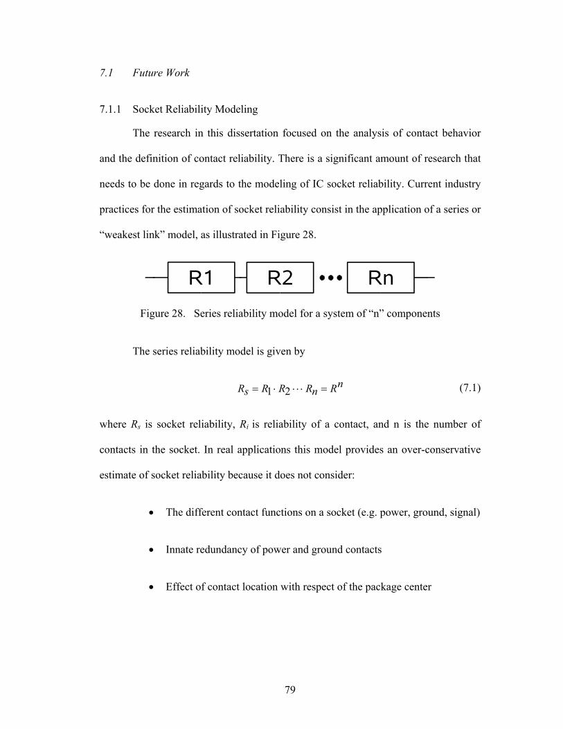
7.1 Future Work
nRnRRRsR 21
7.1.1 Socket Reliability Modeling
The research in this dissertation focused on the analysis of contact behavior
and the definition of contact reliability. There is a significant amount of research that
needs to be done in regards to the modeling of IC socket reliability. Current industry
practices for the estimation of socket reliability consist in the application of a series or
“weakest link” model, as illustrated in Figure 28.
The series reliability model is given by
(7.1)
RnR2R1
Figure 28. Series reliability model for a system of “n” components
where Rs is socket reliability, Ri is reliability of a contact, and n is the number of
contacts in the socket. In real applications this model provides an over-conservative
estimate of socket reliability because it does not consider:
The different contact functions on a socket (e.g. power, ground, signal)
Innate redundancy of power and ground contacts
Effect of contact location with respect of the package center
79

A socket level reliability model should consider the following:
A contact reliability model based on the physics of failure
Failure mechanisms specific to each contact function (e.g. AC, DC,
and signal)
Functional redundancy at package level
Mechanical load variability effects over the surface of the package
Contact position with respect to the package neutral point and number
of contacts at that specific distance
Clustering of failures
7.1.2 Long Term Reliability of Elastomer Sockets
The experiments in this research captured the behavior of elastomer contacts
during the first year of life at nominal operating conditions. Further research is
needed to model the statistical distribution shift over time, which could provide
valuable information on the effects of stress relaxation during the second and third
years after assembly. Since accelerating the aging of the contact by means of
temperature conditions is not a feasible solution, experimental work is needed to
correlate the degradation of elastomer contacts to normal operating conditions,
possibly by means of power cycling and/or temperature cycling experiments.
80
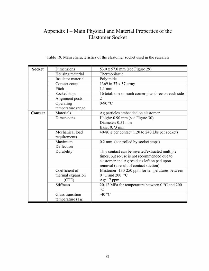
Appendix I – Main Physical and Material Properties of the Elastomer Socket
Table 19. Main characteristics of the elastomer socket used in the research
Dimensions 53.0 x 57.0 mm (see Figure 29) Housing material Thermoplastic Insulator material Polyimide Contact count 1369 in 37 x 37 array Pitch 1.1 mm Socket stops 16 total: one on each corner plus three on each side Alignment posts 2
Socket
Operating temperature range
0-90 °C
Materials Ag particles embedded on elastomer Dimensions Height: 0.90 mm (see Figure 30)
Diameter: 0.51 mm Base: 0.73 mm
Mechanical load requirements
40-80 g per contact (120 to 240 Lbs per socket)
Maximum Deflection
0.2 mm (controlled by socket stops)
Durability This contact can be inserted/extracted multiple times, but re-use is not recommended due to elastomer and Ag residues left on pad upon removal (a result of contact stiction)
Coefficient of thermal expansion (CTE)
Elastomer: 130-250 ppm for temperatures between 0 °C and 200 °C Ag: 17 ppm
Stiffness 20-12 MPa for temperature between 0 °C and 200 °C
Contact
Glass transition temperature (Tg)
-40 °C
81

Figure 29. Illustration of elastomer socket, showing dimensions. The 37 x 37
contact array and main housing features are also shown
Figure 30. Illustration of elastomer contact, showing dimensions. Gray shapes inside
of contact represent Ag particles. Black horizontal region at center of contact represents insulator
82

Appendix II – Analysis of Mechanical Load Applied to IC Socket Assemblies
Mechanical load is a key component in the operating environment of an IC
socket system. If the load is too low, the socket can experience higher contact
resistance values and/or intermittent failures. If the load is too high, the socket can be
physically damaged. A load analysis was performed to quantify the overall applied
conditions for the IC sockets that were utilized in this research.
The component thickness from 20 assembly sets (as shown in Figure 3,
Chapter 2) was measured. As part of the study the constant for each one of the springs
(80 springs total) was obtained by direct measurements using a force tester. The
measurements provided the information needed to estimate the load that was applied
by each test board assembly. The average test board load was found to be 236 Lbs.,
with a standard deviation of 5.7 Lbs. This translates into an average contact load of
78 g, which is within assembly requirement. The results are summarized in Table 20.
83

Table 20. Results of mechanical load analysis
Assembly Total Load (Lbs)
Estimated Load per
Contact (g)
Assembly Total Load (Lbs)
Estimated Load per
Contact (g) 1 232.9 77 11 247.5 82 2 238.6 79 12 237.3 79 3 231.9 77 13 238.0 79 4 232.7 77 14 233.5 77 5 234.2 78 15 226.6 75 6 234.7 78 16 244.8 81 7 230.9 77 17 233.8 77 8 230.4 76 18 233.1 77 9 245.5 81 19 243.4 81 10 236.7 78 20 242.5 80
84

Appendix III – Package and Bolster Plate Shape Analysis
The shape of the daisy chain packages and bolster plates that were used in this
research are important factors in the load and load distribution for IC sockets. The
flatness of a daisy chain package can increase or decrease the amount of load (and of
contact compression) for some socket contacts. The shape of the bolster plate
normalizes the load applied over the whole contact array, reducing high and low load
areas. Shadow Moiré fringe analysis was used to determine the shapes of these
components, allowing the rejection of samples that did not meet assembly
specification. A total of 20 sets were characterized by this method, finding the mean
LGA package flatness to be 3 mils, with a standard deviation of 0.4 mils. The mean
bolster plate flatness was found to be 7 mils with a standard deviation of 1.2 mils. All
samples were found to have acceptable parameters. Representative Shadow Moiré
images are provided in Figures 31 and 32.
Figure 32. Shadow Moiré image for sample bolster plate
Figure 31. Shadow Moiré image for sample package
85

Appendix IV – Sensitivity Analysis of PoF Model Parameters and Model Accuracy Evaluation
The PoF model for the Maxima-SPRT methodology is given by (3.15)
'2''
aeR T
where where Re’ is estimated resistance, ρT’ is resistivity, and a’ is a-spot radius. Both
input parameters are a function of temperature T’. Resistivity, being a material
property, only provides variation on the estimated resistance when the temperature of
the contact changes. To assess the sensitivity of the model to changes in resistivity,
the a-spot radius was set to a constant value (a-spot radius at 20 °C), and the
resistance was calculated from 20 °C to 75 °C, as shown in Figure 33. A 20%
increase in resistivity over temperature (from 1.63E-8 to 1.97E-8 Ω•m) resulted in a
20% increase in resistance (from 4.9 mΩ to 5.9 mΩ).
The a-spot radius contributes to variation of the estimated resistance due to
changes in contact temperature and to errors from the a-spot model (goodness-of-fit
of the model to actual data). To assess the sensitivity of the model to changes in a-
spot radius, the resistivity was set to a constant value (resistivity at 20 °C), and the
resistance was calculated from 20 °C to 75 °C, as shown in Figure 34. A 30%
decrease in a-spot radius over temperature (from 1.67E-6 to 1.18E-6 Ω·m) resulted in
a 40% increase in resistance (from 4.9 mΩ to 6.9 mΩ). The variability of the PoF
model, resulting from a-spot radius estimation errors, was quantified by means of a
repeatability study, where 25 resistance measurements were performed under
86

identical temperature conditions. The estimation error at a fixed temperature was
found to be < 0.1 mΩ.
The model estimates were plotted against resistance measurements to validate
model accuracy, as shown in Figure 35. All model estimates were found to be within
0.1 mΩ from the respective measurement.
Figure 33. Sensitivity of output resistance to changes in resistivity. Resistivity is shown for 20 °C to 75 °C temperature range
87

Figure 34. Sensitivity of output resistance to changes in a-spot radius. Resistivity is shown for 20 °C to 75 °C temperature range
Figure 35. Plot of resistance measurements versus model estimates, validating PoF model accuracy
88
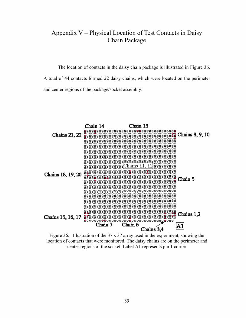
Appendix V – Physical Location of Test Contacts in Daisy Chain Package
The location of contacts in the daisy chain package is illustrated in Figure 36.
A total of 44 contacts formed 22 daisy chains, which were located on the perimeter
and center regions of the package/socket assembly.
Figure 36. Illustration of the 37 x 37 array used in the experiment, showing the location of contacts that were monitored. The daisy chains are on the perimeter and
center regions of the socket. Label A1 represents pin 1 corner
89
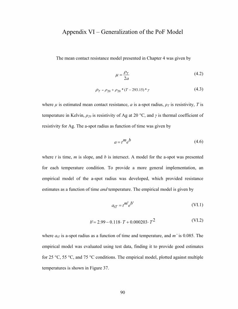
Appendix VI – Generalization of the PoF Model
The mean contact resistance model presented in Chapter 4 was given by
aT
2
(4.2)
(4.3) *)15.293(*2020 TT
where μ is estimated mean contact resistance, a is a-spot radius, ρT is resistivity, T is
temperature in Kelvin, ρ20 is resistivity of Ag at 20 °C, and γ is thermal coefficient of
resistivity for Ag. The a-spot radius as function of time was given by
bemta (4.6)
where t is time, m is slope, and b is intersect. A model for the a-spot was presented
for each temperature condition. To provide a more general implementation, an
empirical model of the a-spot radius was developed, which provided resistance
estimates as a function of time and temperature. The empirical model is given by
'' bemtatT (VI.1)
(VI.2) 2000203.0118.099.2' TTb
where atT is a-spot radius as a function of time and temperature, and m’ is 0.085. The
empirical model was evaluated using test data, finding it to provide good estimates
for 25 °C, 55 °C, and 75 °C conditions. The empirical model, plotted against multiple
temperatures is shown in Figure 37.
90

Figure 37. Plot illustrating the fit of the empirical contact resistance model against test results at 25 °C, 55 °C and 75 °C. Additional curves were created for 45 °C and
65 °C. The model provides good estimates as a function of time and temperature, with a maximum deviation of 0.1 mΩ for the 16 500 h test point at 25 °C
91
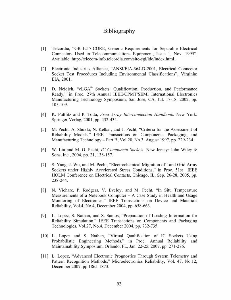
Bibliography
[1] Telcordia, “GR-1217-CORE, Generic Requirements for Separable Electrical Connectors Used in Telecommunications Equipment, Issue 1, Nov. 1995”. Available: http://telecom-info.telcordia.com/site-cgi/ido/index.html .
[2] Electronic Industries Alliance, “ANSI/EIA-364-D-2001, Electrical Connector Socket Test Procedures Including Environmental Classifications”, Virginia: EIA, 2001.
[3] D. Neidich, “cLGA® Sockets: Qualification, Production, and Performance Ready,” in Proc. 27th Annual IEEE/CPMT/SEMI International Electronics Manufacturing Technology Symposium, San Jose, CA, Jul. 17-18, 2002, pp. 105-109.
[4] K. Puttlitz and P. Totta, Area Array Interconnection Handbook. New York: Springer-Verlag, 2001, pp. 432-434.
[5] M. Pecht, A. Shukla, N. Kelkar, and J. Pecht, “Criteria for the Assessment of Reliability Models,” IEEE Transactions on Components, Packaging, and Manufacturing Technology – Part B, Vol.20, No.3, August 1997, pp. 229-234.
[6] W. Liu and M. G. Pecht, IC Component Sockets. New Jersey: John Wiley & Sons, Inc., 2004, pp. 21, 138-157.
[7] S. Yang, J. Wu, and M. Pecht, “Electrochemical Migration of Land Grid Array Sockets under Highly Accelerated Stress Conditions,” in Proc. 51st IEEE HOLM Conference on Electrical Contacts, Chicago, IL, Sep. 26-28, 2005, pp. 238-244.
[8] N. Vichare, P. Rodgers, V. Eveloy, and M. Pecht, “In Situ Temperature Measurements of a Notebook Computer – A Case Study in Health and Usage Monitoring of Electronics,” IEEE Transactions on Device and Materials Reliability, Vol.4, No.4, December 2004, pp. 658-663.
[9] L. Lopez, S. Nathan, and S. Santos, “Preparation of Loading Information for Reliability Simulation,” IEEE Transactions on Components and Packaging Technologies, Vol.27, No.4, December 2004, pp. 732-735.
[10] L. Lopez and S. Nathan, “Virtual Qualification of IC Sockets Using Probabilistic Engineering Methods,” in Proc. Annual Reliability and Maintainability Symposium, Orlando, FL, Jan. 22-25, 2007, pp. 271-276.
[11] L. Lopez, “Advanced Electronic Prognostics Through System Telemetry and Pattern Recognition Methods,” Microelectronics Reliability, Vol. 47, No.12, December 2007, pp 1865-1873.
92

[12] L. Lopez and M. Pecht, “Maxima-SPRT Methodology for Health Monitoring of Contact Resistance in IC Sockets,” in Proc. International Conference on Prognostics and Health Management, Denver, CO, October 6-9, 2008.
[13] K. Whisnant, K. Gross, and N. Lingurovska, “Proactive Fault Monitoring in Enterprise Servers,” in Proc. IEEE International Multiconference in Computer Science and Computer Engineering, Las Vegas, NV, June 27-30, 2005, pp. 3-10.
[14] Y. Lam, C. Maul, and J. McBride, “Temperature, Humidity and Pressure Measurement on Automotive Connectors,” IEEE Transactions on Components and Packaging Technologies, Vol.29, Issue 2, June 2006, pp. 333-340.
[15] R. Holm, Electric Contacts, Theory and Applications. New York: Springer, 2000, pp. 114-116.
[16] K. Whisnant, R. Dhanekula, and K. Gross, “Efficient Signal Selection for Nonlinear System-Based Models of Enterprise Servers,” in Proc. Third IEEE International Workshop on Engineering of Autonomic & Autonomous Systems (EASe’06), Potsdam, Germany, March 27-30, 2006, pp. 141-148.
[17] K. Vaidyanathan, K. Gross, and R. Dhanekula, “Incipient Fault Detection in Storage Systems Using On-line Pattern Recognition,” in Proc. Machinery Failure Prevention Technology Conference (MFPT-60), Virginia Beach, VA, April 26-30, 2006, pp. 101-110.
[18] R. Schmidth and H. Shaukatullah, “Computer and Telecommunications Equipment Room Cooling: A Review of Literature,” IEEE Transactions on Components and Packaging Technologies, Vol.26, No.1, March 2003, pp. 89-98.
[19] L. Lopez and M. Pecht, “Assessing the Operating Temperature and Relative Humidity Environment of IC Sockets in Enterprise Servers,” in Proc. International Conference on Prognostics and Health Management, Denver, CO, October 6-9, 2008.
[20] J. Xie, C. Hillman, P. Sandborn, M. Pecht, A. Hassanzadeh, and D. DeDonato, “Assessing the Operating Reliability of Land Grid Array Elastomer Sockets,” IEEE Transactions on Components and Packaging Technologies, vol. 23, no. 1, pp. 171-176, Mar. 2000.
[21] W. Liu, M. G. Pecht, and J. Xie, “Fundamental Reliability Issues Associated with a Commercial Particle-in-Elastomer Interconnection System,” IEEE Transactions on Components and Packaging Technologies, vol. 24, no. 3, pp. 520-525, Sep. 2001.
[22] J. Hofmeister, P. Lall, D. Goodman, E. Ortiz, M. Adams, and T. Tracy, “Intermittency Detection and Mitigation in Ball Grid Array (BGA) Packages,”
93

[23] M. G. Pecht, Prognostics and Health Management of Electronics. New York: John Wiley & Sons, Inc., 2008.
[24] Electronic Industries Alliance, “EIA/ECA-364-23C, Low Level Contact Resistance Test Procedure for Electrical Connectors and Sockets,” Virginia: EIA, 2006.
[25] H. Qi, N. Vichare, M. Azarian, and M. G. Pecht, “Analysis of Solder Joint Failure Criteria and Measurement Techniques in the Qualification of Electronic Products,” IEEE Transactions on Components and Packaging Technologies, vol. 31, no. 2, pp. 469-477, Jun. 2008.
[26] P. Lall, M. G. Pecht, and E. Hakim, Influence of Temperature on Microelectronics and System Reliability: A Physics of Failure Approach. New York: CRC Press LLC, 1997, pp. 12.
[27] P. Tobias and D. Trindade, Applied Reliability. New York: Chapman & Hall/CRC Press, 1998, pp. 187.
[28] J.A. Fulton, D. Horton, R. Moore, W. Lambert, S. Jin, R. Opila, R. Sherwood, T. Tiefel, and J. Mottine, “Electrical and Mechanical Properties of a Metal-Filled Polymer Composite for Interconnection and Testing Applications,” in Proc. 39th Electronic Components Conference, Houston, TX, May 22-24, 1989, pp. 71-77.
[29] N. Tunca and G. Rosen, “Environmental Testing of Elastomer Connectors,” In Proc. 38th IEEE HOLM Conference on Electrical Contacts, Chicago, IL, Oct. 18-21, 1992, pp. 249-255.
[30] K. Kim, J. Kim, S. Kim, K. Lee, A. Chen, N. Ahmad, N. Dugbartey, M. Karnezos, S. Tam, Y. Kweon, and R. Pendse, “The Viability of Anisotropic Conductive Film (ACF) as a Flip Chip Interconnection Technology,” In Proc. 50th Electronic Components and Technology Conference, Las Vegas, NV, May 21-24, 2000, pp. 1122-1132.
[31] H. Kristiansen and J. Liu, “Overview of Conductive Adhesive Interconnection Technologies for LCD’s,” IEEE Transactions on Components, Packaging, and Manufacturing Technology – Part A, vol. 21, no. 2, pp. 208-214, Jun. 1998.
[32] S. Mannan, D. Williams, and D. Whalley, “Some Optimum Processing Properties for Anisotropic Conductive Adhesives for Flip Chip Interconnector,” Journal of Materials Science: Materials in Electronics, vol.8, no.4, pp. 223-231, Aug. 1997.
94

[33] K. Keswick, R. German, M. Breen, and R. Nolan, “Compliant Bumps for Adhesive Flip-Chip Assembly,” IEEE Transactions on Components, Packaging, and Manufacturing Technology – Part B, vol. 18, no. 3, pp. 503-510, Aug. 1995.
[34] D. Chang, P. Crawford, J. Fulton, R. McBride, M. Schmidt, R. Sinitski, and C. Wong, “An Overview and Evaluation of Anisotropically Conductive Adhesive Films for Fine Pitch Electronic Assembly,” IEEE Transactions on Components, Hybrids, and Manufacturing Technology, vol. 16, no.8, pp. 828-835, Dec. 1993.
[35] M. Mundlein and J. Nicolics, “Electrical Resistance Modeling of Isotropically Conductive Adhesive Joints,” In Proc. 28th International Spring Seminar on Electronics Technology, Wiener Neustadt, Austria, May. 19-22, 2005, pp. 128-133.
[36] M. Brumbach and J. Nadon, Industrial Electricity, 7th Edition. New York: Thomson/Del Mar Learning, 2005, pp. 157.
[37] A. Clauset, C. Shalizi, and M. Newman. (2007, June). Power-law Distributions in Empirical Data. ArXiv eprint. Volume 706, Available: http://arxiv.org/abs/0706.1062
[38] L. Lopez, V. Challa, and M. Pecht, “Assessing the Reliability of Elastomer Sockets in Temperature Environments,” IEEE Transactions on Device and Materials Reliability, vol. 9, no. 1, pp. 80-86, March 2009.
[39] M. J. Nicolics, “Electrical Resistance Modeling of Isotropically Conductive Adhesive Joints,” In Proc. 28th International Spring Seminar on Electronics Technology, Wiener Neustadt, Austria, May. 19-22, 2005, pp. 128-133.
[40] P. S. Slade, Electrical Contacts: Principles and Applications. New York: Marcel-Dekker, Inc., 1999, pp. 1-14.
[41] W. Liu, M. Lee, M. Pecht, and R. Martens, “An Investigation of the Contact Resistance of a Commercial Elastomer Interconnect Under Thermal and Mechanical Stresses,” IEEE Transactions on Device and Materials Reliability, vol. 3, no. 2, pp. 39-43, Jun. 2003.
[42] S. Yang, J. Wu, D. Tsai, and M. G. Pecht, “Contact Resistance Estimation for Time-Dependent Silicone Elastomer Matrix of Land Grid Array Socket,” IEEE Transactions on Components and Packaging Technologies, vol. 30, no. 1, pp. 81-85, Mar. 2007.
[43] J. Xie, M. Pecht, D. DeDonato, and A. Hassanzadeh, “An Investigation of the Mechanical Behavior of Conductive Elastomer Interconnects,” Microelectronics Reliability, vol. 41, no. 2, pp. 281-286, Dec. 2001.
95

96
[44] W. Liu, “Reliability Assessment of Metal Particle-in-Elastomer Sockets,” Ph.D. dissertation, Dept. Mech. Eng., University of Maryland, College Park, MD, 2001.
[45] W. Meeker and L. Escobar, Statistical Methods for Reliability Data. New York: Wiley Inter-science, 1998, pp. 475.
[46] W. Nelson, Accelerated Testing: Statistical Models, Test Plans, and Data Analysis. New York: Wiley, 2004, pp. 79-82.
[47] R. L. Edgeman, “Assessing the Inverse Gaussian Distribution,” IEEE Transactions on Reliability, vol. 39, no. 3, pp. 353-355, Aug. 1990.
[48] R. S. Chhikara and L. Folks, The Inverse Gaussian Distribution: Theory, Methodology, and Applications. New York: Marcel-Dekker Inc., 1989, pp. 71-74.
[49] National Institute of Standards and Technology, “Engineering Statistics Handbook”. Available: http://www.itl.nist.gov/div898/handbook/eda/section3/eda35g.htm.
[50] D. Kececioglu, Reliability and Life Testing Handbook. Pennsylvania: DESTech Publications, 2002, pp. 725-728.
[51] M. Brumbach and J. Nadon, Industrial Electricity, 7th Edition. New York: Thomson/Del Mar Learning, 2005, pp. 157.
[52] R. Mroczkowski and J. Maynard, “Estimating the Reliability of Electrical Connectors,” IEEE Transactions on Reliability, Vol.40, No.5, December 1991, pp. 507-512.
[53] R. Mroczkowski, “Concerning Reliability Modeling of Connectors,” in Proc. 54th IEEE HOLM Conference on Electrical Contacts, Arlington, VA, Oct. 26-28, 1998, pp. 57-68.
[54] R. Timsit, “Electrical Conduction Through Small Contact Spots,” IEEE Transactions on Components and Packaging Technologies, Vol.29, No.4, December 2006, pp. 727-734.
[55] D. Harris and M. Pecht, “A Reliability Study of Fuzz Button Interconnects,” Microelectronics Reliability, Vol.36, No.4, April 1996, pp. 550-557.
[56] M. Modarres, M. Kaminskiy, and V. Krivtsov, Reliability Engineering and Risk Analysis, A Practical Guide. New York: Marcel/Dekker, Inc., 1999, pp. 408.