quadratic programming
TRANSCRIPT

Geometric
Programming for
Communication
Systems

GeometricProgramming forCommunication
Systems
Mung Chiang
Electrical Engineering DepartmentPrinceton University, Princeton
New Jersey 08544, USA
Boston – Delft

Foundations and Trends R© inCommunications and Information Theory
Published, sold and distributed by:now Publishers Inc.PO Box 1024Hanover, MA 02339USATel. +1 781 871 [email protected]
Outside North America:now Publishers Inc.PO Box 1792600 AD DelftThe NetherlandsTel. +31-6-51115274
A Cataloging-in-Publication record is available from the Library of Congress
Printed on acid-free paper
ISBN: 1-933019-09-3; ISSNs: Paper version 1567-2190; Electronic ver-sion 1567-2328c© 2005 M. Chiang
All rights reserved. No part of this publication may be reproduced,stored in a retrieval system, or transmitted in any form or by anymeans, mechanical, photocopying, recording or otherwise, without priorwritten permission of the publishers.
now Publishers Inc. has an exclusive license to publish this mate-rial worldwide. Permission to use this content must be obtained fromthe copyright license holder. Please apply to now Publishers, PO Box179, 2600 AD Delft, The Netherlands, www.nowpublishers.com; e-mail:[email protected]

Contents
1 Introduction 1
1.1 Geometric Programming and Applications 11.2 Nonlinear Optimization of Communication Systems 31.3 Overview 51.4 Notation 6
2 Geometric Programming 9
2.1 Formulations 92.2 Extensions 202.3 Algorithms 35
3 Applications in Communication Systems 47
3.1 Information Theory 473.2 Coding and Signal Processing 663.3 Network Resource Allocation 743.4 Network Congestion Control 963.5 Queuing Theory 107
v
vi Contents
4 Why Is Geometric Programming Useful forCommunication Systems 115
4.1 Stochastic Models 1154.2 Deterministic Models 124
A History of Geometric Programming 131
B Some Proofs 133
B.1 Proof of Theorem 3.1 133B.2 Proof of Corollary 3.1 135B.3 Proof of Theorem 3.2 135B.4 Proof of Proposition 3.3 137B.5 Proof of Theorem 3.4 138B.6 Proof of Theorem 3.5 139B.7 Proof of Proposition 4.1 144B.8 Proof of Proposition 4.2 145B.9 Proof of Theorem 4.1 146
Acknowledgements 147
References 149

1Introduction
1.1 Geometric Programming and Applications
Geometric Programming (GP) is a class of nonlinear optimization withmany useful theoretical and computational properties. Although GPin standard form is apparently a non-convex optimization problem, itcan be readily turned into a convex optimization problem, hence alocal optimum is also a global optimum, the duality gap is zero undermild conditions,1 and a global optimum can be computed very effi-ciently. Convexity and duality properties of GP are well understood,and large-scale, robust numerical solvers for GP are available. Further-more, special structures in GP and its Lagrange dual problem lead tocomputational acceleration, distributed algorithms, and physical inter-pretations.
GP substantially broadens the scope of Linear Programming (LP)applications, and is naturally suited to model several types of impor-tant nonlinear systems in science and engineering. Since its inception
1 Consider the Lagrange dual problem of a given optimization problem. Duality gap is thedifference between the optimized primal objective value and the optimized dual objectivevalue.
1

2 Introduction
in 1960s,2 GP has found applications in mechanical and civil engi-neering, chemical engineering, probability and statistics, finance andeconomics, control theory, circuit design, information theory, codingand signal processing, wireless networking, etc. For areas not relatedto communication systems, a very small sample of some of the GPapplication papers include [1, 24, 29, 38, 43, 44, 53, 57, 64, 65, 58,92, 93, 104, 107, 112, 123, 125, 128]. Detailed discussion of GP canbe found in the following books, book chapters, and survey articles:[52, 133, 10, 6, 51, 103, 54, 20]. Most of the applications in the 1960sand 1970s were in mechanical, civil, and chemical engineering. After arelatively quiet period in GP research in the 1980s and early to mid-1990s, GP has generated renewed interest since the late 1990s.
Over the last five years, GP has been applied to study a variety ofproblems in the analysis and design of communication systems, acrossmany ‘layers’ in the layered architecture, from information theory andqueuing theory to signal processing and network protocols. We alsostart to appreciate why, in addition to how, GP can be applied to asurprisingly wide range of problems in communication systems. Theseapplications have in turn spurred new research activities on the theoryand algorithms of GP, especially generalizations of GP formulationsand distributed algorithms to solve GP in a network. This is a sys-tematic survey of the applications of GP to the study of communica-tion systems. It collects in one place various published results in thisarea, which are currently scattered in several books and many researchpapers, as well as a couple of unpublished results.
Although GP theory is already well-developed and very efficientGP algorithms are currently available through user-friendly softwarepackages (e.g., MOSEK [129]), researchers interested in using GP stillneed to acquire the non-trivial capability of modelling or approximatingengineering problems as GP. Therefore, in addition to the focus on theapplication aspects in the context of communication systems, this sur-vey also provides a rather in-depth tutorial on the theory, algorithms,and modeling methods of GP.
2 Appendix A briefly describes the history of GP.

1.2. Nonlinear Optimization of Communication Systems 3
1.2 Nonlinear Optimization of Communication Systems
LP and other classical optimization techniques have found importantapplications in communication systems for several decades (e.g., as sur-veyed in [15, 56]). Recently, there have been many research activitiesthat utilize the power of recent developments in nonlinear convex opti-mization to tackle a much wider scope of problems in the analysis anddesign of communication systems.
These research activities are driven by both new demands in thestudy of communications and networking, and new tools emerging fromoptimization theory. In particular, a major breakthrough in optimiza-tion over the last two decades has been the development of powerfultheoretical tools, as well as highly efficient computational algorithmslike the interior-point methods (e.g., [12, 16, 17, 21, 97, 98, 111]), fornonlinear convex optimization, i.e., minimizing a convex function sub-ject to upper bound inequality constraints on other convex functionsand affine equality constraints:
minimize f0(x)subject to fi(x) ≤ 0, i = 1, 2, . . . , m
Ax = cvariables x ∈ Rn.
(1.1)
The constant parameters are A ∈ Rl×n and c ∈ Rl. The objectivefunction f0 to be minimized and m constraint functions {fi} are convexfunctions.
From basic results in convex analysis [109], it is well known thatfor a convex optimization problem, a local minimum is also a globalminimum. The Lagrange duality theory is also well developed for con-vex optimization. For example, the duality gap is zero under constraintqualification conditions, such as Slater’s condition [21] that requiresthe existence of a strictly feasible solution to nonlinear inequality con-straints. When put in an appropriate form with the right data struc-ture, a convex optimization problem is also easy to solve numericallyby efficient algorithms, such as the primal-dual interior-point methods[21, 97], which has worst-case polynomial-time complexity for a largeclass of functions and scales gracefully with problem size in practice.

4 Introduction
Special cases of convex optimization include convex QuadraticProgramming (QP), Second Order Cone Programming (SOCP), andSemidefinite Programming (SDP), as well as seemingly non-convexoptimization problems that can be readily transformed into convexproblems, such as GP. Some of these are covered in recent books onconvex optimization, e.g., [12, 16, 17, 21, 97, 98]. While SDP and itsspecial cases of SOCP and convex QP are now well-known in manyengineering disciplines, GP is not yet as widely appreciated. This sur-vey aims at enhancing the awareness of the tools available from GP inthe communications research community, so as to further strengthenGP’s appreciation–application cycle, where more applications (and theassociated theoretical, algorithmic, and software developments) arefound by researchers as more people start to appreciate the capa-bilities of GP in modeling, analyzing, and designing communicationsystems.
There are three distinctive characteristics in the nonlinear optimiza-tion framework for the study of communication systems:
• First, the watershed between efficiently solvable optimizationproblems and intractable ones is being recognized as ‘convex-ity’, instead of ‘linearity’ as was previously believed.3 Thishas opened up opportunities on many nonlinear problems incommunications and networking based on more accurate orrobust modeling of channels and complex interdependencyin networks. Inherently nonlinear problems in informationtheory may also be tackled.
• Second, the nonlinear optimization framework integrates var-ious protocol layers into a coherent structure, providing aunified view on many disparate problems, ranging from clas-sical Shannon theory on channel capacity and rate distortion[33] to Internet engineering such as inter-operability betweenTCP Vegas and TCP Reno congestion control [119].
• Third, some of these theoretical insights are being put intopractice through field trials and industry adoption. Recent
3 In some cases, global solutions and systematic relaxation techniques for non-convex opti-mization have also matured [101, 106].

1.3. Overview 5
examples include optimization-theoretic improvements ofTCP congestion control [71] and DSL broadband access [118].
The phrase “nonlinear optimization of communication systems” infact carries three different meanings. In the most straightforward way,an analysis or design problem in a communication system may be for-mulated as either minimizing a cost or maximizing a utility functionover a set of variables confined within a constraint set. In a more subtleand recent approach, a given network protocol may be interpreted as adistributed algorithm solving an implicitly defined global optimizationproblem. In yet another approach, the underlying theory of a networkcontrol method or a communication strategy may be generalized usingnonlinear optimization techniques, thus extending the scope of appli-cability of the theory. In Section 3, we will see that GP applicationscover all three categories.
1.3 Overview
There are three main sections in this survey. Section 2 is a tutorial ofGP: its basic formulations, convexity and duality properties, variousextensions that significantly broaden the scope of applicability of thebasic formulations, as well as numerical methods, robust solutions, anddistributed algorithms for GP. Although this section does not cover anyapplication topic, it is essential for modeling communication systemproblems in terms of GP and its generalizations.4
Section 3 is the core of this survey, presenting many applications ofGP in the analysis and design of communication systems: the informa-tion theoretic problems of channel capacity, rate distortion, and errorexponent in Subsection 3.1, construction of channel codes, relaxationof source coding problems, and digital signal processing algorithms forphysical layer transceiver design in Subsection 3.2, network resourceallocation algorithms such as power control in wireless networks in Sub-section 3.3, network congestion control protocols in TCP Vegas and itscross-layer extensions in Subsection 3.4, and performance optimizationof simple queuing systems in Subsection 3.5.
4 For another very recent GP tutorial, readers are referred to a recent survey of GP forcircuit design problems [20].

6 Introduction
These applications generally fall into three categories: analysis (e.g.,GP is used to characterize and bound information theoretic limits),forward engineering (e.g., GP is used to control transmit powers inwireless networks), and reverse engineering (e.g., GP is used to modelcongestion control or Highly Optimized Tolerance systems).
Then Section 4 explains why, rather than just how, GP can beapplied to such a variety of problems in communication systems. Asshown in Subsection 4.1, for problems based on stochastic models, GPis often applicable because large deviation bounds can be computed byGPs. As shown in Subsection 4.2, for problems based on determinis-tic models, reasons for applicability of GP is less well understood butmay be due to GP’s connections with proportional allocation, generalmarket equilibrium, and generalized coding problems.
In the area of GP applications for communication systems, there arethree most interesting directions of future research in author’s view:distributed algorithms and heuristics for solving GP in a network, asystematic theory of using a nested family of GP relaxations for non-convex, generalized polynomial optimization, and the connections ofGP with the theories of large deviation and general market equilibrium.These issues are discussed throughout the survey.
Some subsections in these three sections present unpublished resultswhile most subsections summarize known results. In particular, Sub-section 2.1 is partially based on [10, 21, 30, 52, 132], Subsection 2.2 on[6, 7, 10, 20, 51, 52, 103, 133], Subsection 2.3 on [21, 60, 67, 78, 37],Subsection 3.1 on [30, 33, 42, 82, 84, 120, 121, 122], Subsection 3.2on [25, 30, 69, 75, 91], Subsection 3.3 on [37, 34, 35, 72, 73], Subsec-tion 3.4 on [31, 88], Subsection 3.5 on [36, 68, 76], Subsection 4.1 on[30, 42, 45, 52, 108], and Subsection 4.2 on [28, 49, 70].
A brief historical account of the development of GP is provided inAppendix A and selected proofs are provided in Appendix B.
1.4 Notation
We will use the following notation. Vectors and matrices are denoted inboldface. Given two column vectors x and y of length n, we express thesum
∑ni=1 xiyi as an inner product xTy. Componentwise inequalities

1.4. Notation 7
on a vector x with n entries are expressed using the � symbol: x � 0denotes xi ≥ 0, i = 1, 2, . . . , n. A column vector with all entries being 1is denoted as 1. We use Rn
+ and Rn++ to denote the non-negative and
strictly positive quadrant of n-dimensional Euclidean space, respec-tively, and Z+ to denote the set of non-negative integers.
Sometimes a symbol has different meanings in different sections,because the same symbol is widely accepted as the standard notationrepresenting different quantities in more than one field. For example,P denotes channel transition matrix in Subsection 3.1.1 on channelcapacity, and denotes transmit power vector in Subsections 3.3.1 and3.4.2 on wireless network power control. Such notational reuse shouldnot cause any confusion since consistency is maintained within anysingle subsection.
All constrained optimization problems are written in this surveyfollowing a common format: objective function, constraints, and opti-mization variables. Constant parameters are also explicitly stated afterthe problem statement in cases where confusion may arise.

2Geometric Programming
2.1 Formulations
2.1.1 Basic formulations and convexity property
There are two equivalent forms of GP: standard form and convexform. The first is a constrained optimization of a type of functioncalled posynomial, and the second form is obtained from the firstthrough a logarithmic change of variable. Standard form GP is oftenused in network resource allocation problems, and convex form GPin problems based on stochastic models such as information theoreticproblems.
We first define a monomial as a function f : Rn++ → R:1
f(x) = dxa(1)
1 xa(2)
2 · · ·xa(n)
n
1 Since the domain of monomials is the strictly positive quadrant of Rn, when a GP iswritten in terms of monomials, it is implicitly assumed that the optimal variables cannotbe zero. In theory, there is a loss of generality in this assumption for some applications.Numerically, this assumption may not introduce any difficulty since the interior-pointmethod solves a GP through a feasible path inside the constraint set.
9

10 Geometric Programming
where the multiplicative constant d ≥ 0 and the exponential constantsa(j) ∈ R, j = 1, 2, . . . , n. A sum of monomials, indexed by k below, iscalled a posynomial:
f(x) =K∑
k=1
dkxa(1)k
1 xa(2)k
2 · · ·xa(n)k
n .
where dk ≥ 0, k = 1, 2, . . . , K, and a(j)k ∈ R, j = 1, 2, . . . , n, k =
1, 2, . . . , K. The key features about a posynomial, which will beexplained and utilized many places throughout this survey, are its pos-itivity and convexity (in log domain).
For example, 2x−π1 x0.5
2 + 3x1x1003 is a posynomial in x, x1 − x2 is
not a posynomial, and x1/x2 is a monomial, thus also a posynomial.Minimizing a posynomial subject to posynomial upper bound
inequality constraints and monomial equality constraints is called ageometric program in standard form:2
minimize f0(x)subject to fi(x) ≤ 1, i = 1, 2, . . . , m
hl(x) = 1, l = 1, 2, . . . , M
variables x
(2.1)
where fi, i = 0, 1, . . . , m, are posynomials:
fi(x) =Ki∑k=1
dikxa(1)ik
1 xa(2)ik
2 · · ·xa(n)ik
n ,
and hl, l = 1, 2, . . . , M are monomials:
hl(x) = dlxa(1)l
1 xa(2)l
2 · · ·xa(n)l
n .
Note that a monomial equality constraint can also be expressed astwo monomial inequality constraints: hl(x) ≥ 1 and 1/hl(x) ≤ 1. Thusa standard form GP can be defined as the minimization of a posynomialunder upper bound inequality constraints on posynomials.
2 Another name that is often used is ‘posynomial form’.

2.1. Formulations 11
Given a GP in standard form, we can form a matrix A where eachrow consists of the exponential constants associated with each mono-mial term that appears in the objective and constraints, and a vector dconsisting of all the multiplicative constants. Each GP can be uniquelyrepresented by the following data structure: A, d, and an identificationof which rows in A and d belong to the objective function and whichto each of the constraint functions.
As a small example, consider the following GP in standard form,with variables (x, y, z):3
minimize xy + xz
subject to 0.8√
yzx2 ≤ 1
0.5√xy
≤ 11x ≤ 1
variables x, y, z.
(2.2)
The constant parameters of this GP are:
A =
1 1 01 0 1
−2 1/2 1/2−1/2 −1 0−1 0 0
and
d = [1, 1, 0.8, 0.5, 1]T
where the first two rows in A and d correspond to the two monomialterms in the objective function, and the last three rows each corre-sponds to a constraint.
GP in standard form is not a convex optimization problem, becauseposynomials are not convex functions. However, with a logarithmicchange of all the variables and multiplicative constants: yi = log xi,
3 We will show in Subsection 3.1.1 that this GP is in fact computing a channel capacitywith an input cost constraint.

12 Geometric Programming
bik = log dik, bl = log dl, we can turn it into the following problem:
minimize∑K0
k=1 exp(aT0ky + b0k)
subject to∑Ki
k=1 exp(aTiky + bik) ≤ 1, i = 1, 2, . . . , m
aTl y + bl = 0, l = 1, 2, . . . , M
variables y
where aik = [a(1)ik , a
(2)ik , . . . , a
(n)lk ]T , which is obviously equivalent4 to the
following GP in convex form:
minimize p0(y) = log∑K0
k=1 exp(aT0ky + b0k)
subject to pi(y) = log∑Ki
k=1 exp(aTiky + bik) ≤ 0,
i = 1, 2, . . . , m
ql(y) = aTl y + bl = 0, l = 1, 2, . . . , M
variable y.
(2.3)
For the small example (2.2) of GP in standard form, the followingproblem is its convex form in x = log x, y = log y, z = log z:
minimize log (exp(x + y) + exp(x + z))subject to 0.5y + 0.5z − 2x + log 0.8 ≤ 0
0.5x + y + log 0.5 ≤ 0−x ≤ 0
variables x, y, z.
To show that (2.3) is indeed a convex optimization problem, weneed to show that the objective and inequality constraint functions areconvex in y. This convexity property can be readily verified through apositive-definiteness test of the Hessian. A more illuminating verifica-tion uses a duality argument.
Lemma 2.1. The log-sum-exp function f(x) = log∑n
i=1 exi is convexin x.
4 Equivalence relationship between two optimization problems is used in a loose waythroughout this survey. If the optimized value of problem A is a simple (e.g., mono-tonic and invertible) function of the optimized value of problem B, and an optimizer ofproblem B can be easily computed from an optimizer of problem A (e.g., through a simplemapping), then problems A and B are said to be equivalent.

2.1. Formulations 13
Proof. Consider the following log-sum inequality [42, 40] (readilyproved by the convexity of f(t) = t log t, t ≥ 0):
n∑i=1
ai logai
bi≥
(n∑
i=1
ai
)log
∑ni=1 ai∑ni=1 bi
(2.4)
where a,b � 0.5
Recall that, given a function f : Rn → R, the function f� : Rn →R, defined as
f�(y) = supx∈dom f
(yTx − f(x)), (2.5)
is called the conjugate function of f . Since f� is the pointwise supremumof a family of affine functions of y, it is always a convex function.6
Let bi = log bi and∑n
i=1 ai = 1 in the log-sum inequality (2.4). Weobtain
log
(n∑
i=1
ebi
)≥ aT b −
n∑i=1
ai log ai,
with equality if and only if ai = ebi∑j
ebj. This by definition shows that
the log-sum-exp function is the conjugate function of negative entropy.Since all conjugate functions are convex, the log-sum-exp function isconvex.
The composition of a convex function with an affine function is aconvex function, thus GP in convex form is indeed a convex optimiza-tion: minimizing a convex function subject to upper bound inequalityconstraints on convex functions and affine equality constraints.7
5 This inequality also readily shows the convexity of the Kullback-Leibler divergence, orrelative entropy, between two distributions p,q: D(p‖q) =
∑n
i=1 pi log piqi
in (p,q) [40],which in turn shows that channel capacity and rate distortion problems, to be discussedin Subsection 3.1, are convex optimization problems.
6 As a simple fact to be used in Subsection 4.1.1, it is easy to verify that, if f�(y) is theconjugate of f(x), then for a given T > 0, the perspective function Tf�( y
T) is the conjugate
of the scaled function Tf(x).7 Sum-exp functions are also convex. In GP convex form, we further take the log of thesum-exp functions in the objective and constraints, which turns monomials into affinefunctions and also improves numerical stability of solution algorithms.

14 Geometric Programming
Convexity of the log-sum-exp function can also be verified from thefollowing geometric inequality: the arithmetic mean is greater than orequal to the geometric mean [52]. It is for this reason that the nameof geometric programming was used to describe the class of nonlinearoptimization problems in the form of (2.1) or (2.3).
It is interesting to notice that, in the special case where all theposynomials in a GP in standard form are simply monomials, then thisGP in convex form reduces to a LP. Hence GP can be viewed an anextension of LP.8
Examining GP in convex form, we appreciate why, in the defini-tion of standard form GP, equality constraints can only be imposed onmonomials. If there were posynomial equality constraints (or, equiv-alent, lower bound inequality constraints on posynomials), we wouldhave obtained, after the logarithmic change of variable, a non-convexoptimization problem, because the constraint set would not be convexeven after the transformation. We also appreciate why, in the definitionof posynomial, the exponential constants can be any real numbers (theyappear only in an affine transformation of y), but the multiplicativeconstants must be positive numbers (they need to be logarithmicallytransformed).
Note that although posynomial seems to be a non-convex function,it becomes a convex function after the log transformation, as shownin an example in Figure 2.1. Compared to the (constrained or uncon-strained) minimization of a polynomial, the minimization of a posyno-mial in GP relaxes the integer constraint on the exponential constantsbut imposes a positivity constraint on the multiplicative constants andvariables. There is a sharp contrast between these two problems: poly-nomial minimization is NP-hard, but GP can be turned into convexoptimization with provably polynomial-time algorithms for a globaloptimum.
In an extension of GP called Signomial Programming, which willbe discussed in Subsection 2.2.5, the restriction of non-negative multi-plicative constants is removed, resulting in a general class of nonlinear
8 This extension is different from the extension of LP to (convex) QP, which can be furtherextended to SOCP and SDP. GP is not a special case of SDP.

2.1. Formulations 15
05
10
0
5
10
0
20
40
60
80
100
120
YX
Fun
ctio
n
02
4
0240.5
1
1.5
2
2.5
3
3.5
4
4.5
5
AB
Fun
ctio
n
Fig. 2.1 A bi-variate posynomial before (left graph) and after (right graph) the log trans-formation. A non-convex function is turned into a convex one.
and truly non-convex problems that is simultaneously a generalizationof GP and polynomial minimization over the positive quadrant, as sum-marized in the comparison Table 2.1.
GP PMoP SPc R+ R R
a(j) R Z+ Rxj R++ R++ R++
Table 2.1 Comparison of GP, constrained polynomial minimization over the positive quad-rant (PMoP), and Signomial Programming (SP). All three types of problems minimize asum of monomials subject to upper bound inequality constraints on sums of monomials,but have different definitions of monomial: c
∏j
xa(j)
j . GP is known to be polynomial-timesolvable, but PMoP and SP are not.
The objective function of Signomial Programming can be formu-lated as minimizing a ratio between two posynomials, which is not aposynomial since posynomials are closed under positive multiplicationand addition but not division. As shown in Figure 2.2, a ratio between

16 Geometric Programming
two posynomials is a non-convex function both before and after thelog transformation. Although it does not seem likely that SignomialProgramming can be turned into a convex optimization problem, thereare heuristics to solve it through a sequence of GP relaxations. Suchmethods current lack and would benefit significantly from a theoreticalfoundation similar to the sum-of-squares method [101, 102], which usesa nested family of SDP relaxations to solve constrained polynomialminimization problems.
0
5
10
0
5
10−20
0
20
40
60
XY
Fun
ctio
n
0
1
2
3
0
1
2
32
2.5
3
3.5
AB
Fun
ctio
n
Fig. 2.2 Ratio between two bi-variate posynomials before (left graph) and after (right graph)the log transformation. It is a non-convex function in both cases.
2.1.2 Lagrange duality
The last subsection shows that a GP is a nonlinear, seemingly non-convex optimization problem that can be transformed into a nonlinear,convex problem. Therefore, a local optimum for GP is also a globaloptimum, and the duality gap is zero under mild technical conditions.The Lagrange dual problem of GP has interesting structures. In par-ticular, dual GP is linearly constrained and its objective function is ageneralized entropy function.

2.1. Formulations 17
Following the standard procedure of deriving the Lagrange dualproblem [21], it is readily verified that for the following GP with m
posynomial constraints,
minimize log∑K0
k=1 exp(aT0ky + b0k)
subject to log∑Ki
k=1 exp(aTiky + bik) ≤ 0, i = 1, . . . , m
variables y,
the Lagrange dual problem is
maximize bT0 ν0 − ∑K0
j=1 ν0j log ν0j
+∑m
i=1
(bT
i νi − ∑Kij=1 νij log νij
1T νi
)subject to νi � 0, i = 0, . . . , m
1T ν0 = 1∑mi=0 AT
i νi = 0variables νi, i = 0, 1, . . . , m.
(2.6)
The length of νi is Ki, i.e., the number of monomial terms in the ithposynomial, i = 0, 1, . . . , m. Here, A0 is the matrix of the exponentialconstants in the objective function, where each row corresponds toeach monomial term (i.e., aT
0k is the kth row in matrix A0), andAi, i = 1, 2, . . . , m, are the matrices of the exponential constantsin the constraint functions, again with each row corresponding to eachmonomial term. The multiplicative constants in the objective functionare denoted as b0 and those in the ith constraint as bi, i = 1, 2, . . . , m.
For the example GP (2.2) in the last subsection, its Lagrange dualproblem is the following linearly constrained concave maximization:
maximize ν01 + ν02 − ν01 log ν01 − ν02 log ν02
+ 0.8ν1 + 0.5ν2 + ν3 − ν1 log ν1 − ν2 log ν2 − ν3 log ν3
subject to ν0j ≥ 0, j = 1, 2νi ≥ 0, i = 1, 2, 3ν01 + ν02 = 1A0ν0 + A1ν1 + A2ν2 + A3ν3 = 0
variables ν01, ν02, ν1, ν2, ν3
where A0 = [1, 1, 0; 1, 0, 1],A1 = [−2, 1/2, 1/2],A2 =[−1/2, −1, 0],A3 = [−1, 0, 0].

18 Geometric Programming
A special case is unconstrained GP:
minimizey logN∑
i=1
exp(aTi y + bi).
From (2.6), the Lagrange dual problem of unconstrained GP reducesto
maximize bT ν − ∑Ni=1 νi log νi
subject to 1T ν = 1ν � 0AT ν = 0
variables ν.
(2.7)
The first two constraints imply that the dual variable ν must be a prob-ability distribution. The dual problem (2.7) is a linearly constrainedmaximization of the entropy of distribution ν plus a linear term bT ν.
The Lagrange dual problem (2.6) of a constrained GP can be inter-preted as follows. Dual variable vector ν0 is normalized but other dualvariable vectors νi, i = 1, 2, . . . , m, are not, and the objective functionis a sum of linear terms and ‘generalized’ entropies of νi (which arenot normalized except when i = 0), to be maximized under a linearequality constraint where the weights are the exponential constants inthe posynomials. The relationship between GP and free energy opti-mization in statistical physics will be discussed in Subsection 4.1.1.
By weak duality, any feasible solution of the dual GP, which can beeasily computed by finding a solution to a system of linear inequalities,lower bounds the primal GP’s optimal value. By strong duality, whichholds for any GP in convex form that has a strictly feasible solution,the duality gap between a GP and its dual is zero. The optimal dualvariables, as often is the case for convex optimization problems, providevery useful information about the sensitivity of the optimal solution todata perturbation and the tightness of a constraint at optimality.
2.1.3 Feasibility and sensitivity analysis
Testing whether there is any x that satisfies a set of posynomial inequal-ity and monomial equality constraints:
fi(x) ≤ 1, i = 1, . . . , m, hl(x) = 1, l = 1, . . . , M, (2.8)

2.1. Formulations 19
is called a GP feasibility problem. Solving a feasibility problem isuseful when we would like to determine whether the constraints aretoo tight to allow any feasible solution, or when it is necessary togenerate a feasible solution as the initial point of a interior-pointalgorithm.
Feasibility of the monomial equality constraints can be verified bychecking feasibility of the linear system of equations that the mono-mial constraints get transformed into. Feasibility of the posynomialinequality constraints can then be verified by solving the following GP,introducing an auxiliary variable s ∈ R in addition to variables x ∈ Rn
[52, 20]:
minimize s
subject to fi(x) ≤ s, i = 1, . . . , m
s ≥ 1variables x, s.
(2.9)
This GP always has a feasible solution: s = max{1, maxi{fi(x)}} forany x that satisfies the monomial equality constraints. Now solve prob-lem (2.9) and obtain the optimal (s∗,x∗). If s∗ = 1, then the set ofposynomial constraints fi(x) ≤ 1 is feasible, and the associated x∗ isa feasible solution to the original feasibility problem (2.9). Otherwise,the set of posynomial constraints is infeasible.
The constant parameters in a GP may be based on inaccurate esti-mates or vary over time. As constant parameters change a little, wemay not want to solve the slightly perturbed GP from scratch. It isuseful to directly determine the impact of small perturbations of con-stant parameters on the optimal solution. Suppose we loosen the 1thinequality constraint (with u1 > 0) or tighten it (with ui < 0), andshift the lth equality constraint (with vl ∈ R):
minimize f0(x)subject to fi(x) ≤ eui , i = 1, . . . , m
hl(x) = evl , l = 1, . . . , M
variables x.
(2.10)

20 Geometric Programming
Consider the optimal value of a GP p∗ as a function of the perturba-tions (u,v). The sensitivities of a GP with respect to the ith inequalityconstraint and lth equality constraint are defined as:
Si =∂ log p∗(0, 0)
∂ui=
∂p∗(0, 0)/∂ui
p∗(0, 0),
Tl =∂ log p∗(0, 0)
∂vl=
∂p∗(0, 0)/∂vl
p∗(0, 0).
A large sensitivity Si with respect to an inequality constraint meansthat if the constraint is tightened (or loosened), the optimal value ofGP increases (or decreases) considerably. Sensitivity can be obtainedfrom the corresponding Lagrange dual variables of (2.10): Si = −λi andTl = −νl where λ and ν are the Lagrange multipliers of the inequalityand equality constraints in the convex form of (2.10), respectively.
There are also systematic procedures [52, 46, 48, 80] to obtain theoptimizer x∗ of the perturbed GP (2.10), without solving the perturbedproblem from scratch, based on the constant parameter perturbations(u,v), and the exponent constant matrix A, and multiplicative con-stant vector d.
2.2 Extensions
The scope of GP formulations can be substantially expanded beyondthe basic formulation in Section 2.1. We summarize these extensions infive groups in this section:
• Simple transformations by term rearrangements and partialchange of variable.
• Generalized GP that allows compositions of posynomialswith other functions.
• Extended GP based on other geometric inequalities.• GP formulations based on monomial and posynomial approx-
imations of nonlinear functions.• Signomial Programming that allows posynomial equality
constraints.
It is important to note that, unlike the first four groups of exten-sions, Signomial Programming cannot be transformed into convex

2.2. Extensions 21
optimization problems. The third and fourth groups of extensionsenlarge the scope of GP formulations so much that many convex opti-mization problems can fit into the GP framework. In contrast, thefirst and second groups of extensions transform a problem that already‘looks like’ a GP into an equivalent GP in standard form. In the nexttwo sections on GP applications in communication systems, we willprimarily use the transformations in the first and second groups ofextensions.
Unless specified otherwise, f denotes posynomials and g, h denotemonomials in this subsection. When it is clear that x are the variables,we omit the variables field in the data structure of the representationof an optimization problem.
2.2.1 Simple transformations
It is trivial to realize that the following problems are GPs.Extension 1: Maximize a monomial subject to posynomial upper
bound inequality constraints:
maximize h0(x)subject to fi(x) ≤ 1, i = 1, . . . , m
hj(x) = 1, j = 1, . . . , M.
This is still a GP because maximizing a monomial is equivalent to min-imizing its reciprocal, which is another monomial (thus a posynomial):
minimize 1h0(x)
subject to fi(x) ≤ 1, i = 1, . . . , m
hj(x) = 1, j = 1, . . . , M.
Extension 2: The right hand side of poysnomial inequality andmonomial equality constraints can be monomials instead of 1:
minimize f0(x)subject to fi(x) ≤ gi(x), i = 1, . . . , m
hj(x) = gj(x), j = 1, . . . , M.
This is still a GP because by dividing the right hand side monomialon both sides of the constraints, we obtain upper bound inequality

22 Geometric Programming
constraints on the ratio between a posynomial and a monomial (whichis another posynomial) and equality constraints on the ratio betweentwo monomials (which is another monomial):
minimize f0(x)subject to fi(x)
gi(x) ≤ 1, i = 1, . . . , mhj(x)gj(x) = 1, j = 1, . . . , M.
In general, we define an inverted posynomial as the ratio between amonomial and a posynomial. Lower bounding an inverted posynomial isallowed in a GP since it is equivalent to upper bounding a posynomial.
Extension 3: Positive sums and products of posynomials are alsoposynomials. For example,
(xy1/2 + z)(x−1/2 + yz) + xy = x1/2y1/2 + xy2/3z + x−1/2z + yz2 + xy.
Therefore, the objective function and inequality constraint functions ina GP can be any positive sums and products of posynomials.
Suppose the variables of an optimization problem can be separatedinto two sets, and no term in the problem involves variables from morethan one set. If the problem is convex in one set of log-transformedvariables and a convex optimization in the other set of variables, wecan use a log change of variables only for the first set and obtain aconvex optimization (although not a convex form GP). An example isthe following:
Extension 4: An optimization problem is called a Mixed LinearGeometric Programming (MLGP) if with a log change of x vari-ables, the following problem can be turned into a convex optimization:
minimize f0(x) + aT0 y
subject to fi(x) + aTi y + di ≤ 1, i = 1, . . . , m
hj(x) = 1, j = 1, . . . , M
variables x,y.
Extension 5: Consider the following unconstrained minimizationproblem:
minimizem∑
i=1
exp(fi(x)),

2.2. Extensions 23
where fi are posynomials with non-negative exponents. Introducingauxiliary variables ti, we can transform the above problem into thefollowing equivalent problem:
minimize∑m
i=1 exp(ti)subject to fi(x) ≤ ti, i = 1, . . . , m
variables x, t.
At optimality, the inequality constraints will be tight. Now apply a logchange of variable from x to y, the above problem can be turned intoa convex optimization in (y, t). This method of utilizing monotonicityof posynomials with non-negative exponents and introducing auxiliaryvariables is a common one that will also be used in the next subsection.
There are other simple transformations that only require basic arith-metics, such as the following:
Extension 6: Maximizing a sum of log of monomials:
m∑i=1
log(hi(x))
is equivalent to a GP of minimizing the following monomial:
m∏i=1
(h−1i (x)).
2.2.2 Generalized GP
Generalized GP refers to minimizing a generalized posynomial subjectto upper bound inequality constraints on generalized posynomials. Ageneralized posynomial is a composition of the following three func-tions, each of which generalizes the posynomial function.9
Extension 7: Consider composing posynomials {fij(x)} with aposynomial with non-negative exponents {aij}:
F1(x) =∑
i
dj
∏j
faij
ij (x).
9 The term ‘Generalized GP’ is also used by some authors to denote Signomial Programming,which will be discussed in Subsection 2.2.5. In this survey, Generalized GP should not beconfused with Signomial Programming.

24 Geometric Programming
Introducing auxiliary variables tij , we see that minimizing F1(x) isequivalent to the following GP:
minimize∑
i dj∏
j taij
ij
subject to fij(x) ≤ tij , ∀i, j
variables x, {tij}.
This equivalence is due to the monotonicity of posynomials with non-negative exponents. Similarly, an upper bound inequality constrainton F1(x) can be turned into the following posynomial constraints invariables (x, {tij}):
∑i dj
∏j t
aij
ij ≤ 1, fij(x) ≤ tij , ∀i, j. Composingposynomials with a posynomial with non-negative exponents producesa generalized posynomial F1. Posynomial objective and constraints ina GP can be substituted with generalized posynomials in the form ofF1 while maintaining the GP form of the problem.
Extension 8: The maximum of a finite number of posynomials isalso a generalized posynomial, because
minimize F2(x) = maxi
{fi(x)}
is equivalent to the following GP:
minimize t
subject to fi(x) ≤ t, ∀i
variables x, t.
Extension 9: The following function is also a generalized posy-nomial:
F3(x) =f1(x)
h(x) − f2(x)
where f1 and f2 are posynomials and h is a monomial.This is because minimizing F3(x) is equivalent to the following GP:
minimize t
subject to f2(x)h(x) + f1(x)
th(x) ≤ 1variables x, t.
Any combination of composition of F1, F2, F3 is also a generalizedposynomial. Minimizing a generalized posynomial subject to upper

2.2. Extensions 25
bound inequality constraints on generalized posynomials is a General-ized GP, which can be turned into a standard form GP by introducingauxiliary variables as shown above.
As an example, the following problem in x is a generalized GP:
minimize max{(x1 + x−12 )0.5, x1x3} + (x2 + x−2.9
3 )1.5
subject to (x2x3+x2/x1)π
x1x2−max{x21x3
3,x1+x3} ≤ 10
variables x1, x2, x3,
which is equivalent to the following GP:
minimize t1 + t1.52
subject to 0.1(tπ4 + t5)x−11 x−1
2 ≤ 1t0.53 t−1
1 ≤ 1x1x3t
−11 ≤ 1
(x1 + x−12 )t−1
3 ≤ 1(x2 + x−2.9
3 )t−12 ≤ 1
(x2x3 + x2x−11 )t−1
4 ≤ 1x2
1x23t
−15 ≤ 1
(x1 + x3)t−15 ≤ 1
variables x1, x2, x3, t1, t2, t3, t4, t5.
2.2.3 Extended GP
The theory of GP, including the convexity and duality properties, canbe developed from a basic geometric inequality: the arithmetic mean isgreater than or equal to the geometric mean. GP can be extended byother geometric inequalities. This subsection provides a brief introduc-tion to such Extended GP. Further details concerning Extended GPand its refined duality theory can be found in e.g. [52, 6].
The following inequality
xTy ≤ λ(y)G(x) − F (y), (2.11)
for x in an open convex set and y in a cone, is called a geometricinequality if λ(y) is non-negative, G(x) is differentiable, and for everyx there is a y for which the inequality becomes equality.

26 Geometric Programming
Different geometric inequalities lead to different classes of ExtendedGP. The following choice of functions leads to the basic version ofconvex form GP:
G(x) = logn∑
i=1
exp(xi)
λ(y) = 1Ty
F (y) = −n∑
i=1
yi log yi − λ(y) log λ(y).
If y is a probability distribution, i.e., y � 0,1Ty = 1, the above geo-metric inequality reduces to the conjugacy relationship between log-sum-exp function and negative entropy. Indeed, it can be shown thatF (y) is simply the conjugate function of G(x) restricted to the set ofy such that there is an x for which ∇G(x) = y.
In general, geometric inequality and conjugate function are relatedas follows [6]. By scaling the defining equation (2.5) of conjugacy rela-tionship by λ > 0, we have:
xTy ≤ λG(x) + λG�(y/λ)
where G�(y) is the conjugate function of G(x). Now generalize the con-stant λ to a homogeneous positive function λ(y) such that λ(∇G(x)) =1, we have
xTy ≤ λ(y)G(x) + λ(y)G�(y/λ(y)).
Letting F (y) = λ(y)G�(y/λ(y)) recovers the geometric inequality(2.11) from this generalization of the conjugacy relationship.
It can be readily verified [52] that G(x) in a geometric inequality isalways a convex function. Once a geometric inequality is obtained, min-imizing an objective function in the form of G(x) subject to inequalityconstraints on other functions in the form of G(x) is a convex optimiza-tion, called the Extended GP derived from this geometric inequality.In this sense, Extended GP covers a very wide range of convex opti-mization problems. As long as the objective and constraint functionscan be obtained from some geometric inequality, the associated convexoptimization problem is an Extended GP.

2.2. Extensions 27
Not only there is always a convex function accompanying a geo-metric inequality, geometric inequalities can also be constructed fromconvex functions. Suppose a function g(x) is positive, convex, differen-tiable, and homogeneous of degree p > 1. Restrict its domain to be anopen half space with a boundary containing the origin. Let h(y) be theconjugate function of g(x) and let q be such that 1/p + 1/q = 1. Thenthe following geometric inequality, which is an extension of Holder’sinequality, can be constructed [52]:
yTx ≤ (pg(x))1/p(qh(y))1/q.
In particular, given a differentiable (except possibly at the origin)norm, there is a positive, homogeneous function λ(y) such that
yTx ≤ λ(y)‖x‖,
which is a geometric inequality when x is confined to an open half spacewhose boundary contains the origin. This leads to the following:
Extension 10: Minimizing a differentiable norm over an open halfspace whose boundary contains the origin is an Extended GP.
As a more specific example of Extended GP, consider the followinggeometric inequality:
G(x) =N−1∑i=1
exp(xi + log ci) + xN + log cN
λ(y) = yN
F (y) = log yN
(N−1∑i=1
yi
)−
N−1∑i=1
yi(log yi − 1) +N∑
i=1
yi log ci
where c � 0 is a constant vector. This geometric inequality leads tothe following [52]:
Extension 11: Minimizing the sum of a posynomial and the logof a monomial, subject to inequality posynomial constraints, is anExtended GP.
2.2.4 Approximation and fitting
Sometimes an objective or constraint function in an optimization prob-lem is not a posynomial, and we would like to use a monomial or a

28 Geometric Programming
posynomial to approximate the given function so that optimizing orconstraining this function can be accommodated in a GP. Intuitively, afunction f(x) can be accurately approximated by a posynomial if thefunction F (y) = log f(exp(y)) can be accurately approximated by aconvex function.
Consider the simple case of monomial approximation [6, 20]. Weare given a nonlinear function f : Rn → R that is differentiable atx0 0 and f(x0) > 0. We would like to approximate f(x) with amonomial f(x) = c
∏ni=1 xai
i . We use the following log transformation:yi = log xi, g(y) = log f(y), g(y) = log f(y) = log c + aTy. Equatingthe first order Taylor expansion of g at y0 with g(y), we obtain:
g(y0) + ∇g(y0)T (y − y0) = log c + aTy,
which implies thata = ∇g(y0),
i.e.,
ai =xi
f(x)∂f
∂xi
∣∣∣∣x=x0
, ∀i,
and that
c = exp(g(y0) − ∇g(y0)Ty0) = f(x)n∏
i=1
xaii
∣∣∣∣∣x=x0
.
Once a and c are computed, a monomial approximation f(x) to theoriginal nonlinear function f(x) is obtained.
Sometimes we are given a set of empirical data points, which wewould like to curve-fit using monomials, posynomials, or generalizedposynomials. Posynomials and generalized posynomials offer much flex-ibility in fitting empirical data, which can then be used in modeling theproblem in a GP formulation. Methods for monomial and posynomialdata fitting are explained in [20].
A limiting argument can also be used to allow a GP to approximatea nonlinear optimization problem.
Extension 12: Consider an unconstrained minimization of
f(x) + exp(g(x)).

2.2. Extensions 29
Since ez = limφ→∞(1 + z
φ
)φ, the above minimization can be approx-
imated for a large, fixed φ through the following GP, where t is anauxiliary variable:
minimize f(x) + tφ
subject to t−1 + t−1φ−1g(x) ≤ 1variables x, t.
Nonlinear programs that involve both posynomials and exponentials(or logarithms) of posynomials are called Transcendental GP. They arein general not convex optimization problems and the Lagrange dualproblems may not be linearly constrained [6].
2.2.5 Signomial Programming
All of the GP extensions discussed so far (except Transcendental GP)can be converted into convex optimization problems. This subsectionfocuses on Signomial Programming (SP), which is an extension of GPthat in general cannot be turned into convex problems.
In standard form GP, only upper bound inequality constraints areallowed on posynomials. Sometimes a posynomial represents a qualityof service that needs to be lower bounded. Equality constraints onposynomials are also common in network modeling. In particular, flowconservation equality constraints are linear equality constraints. It is alimitation in GP modeling that lower bound inequalities (or equalities)on posynomials are not allowed in standard form GP.
This issue can be tackled by extending GP to SP: minimizing asignomial subject to upper bound inequality constraints on signomi-als, where a signomial is a sum of monomials, possibly with negativemultiplicative coefficients:
s(x) =N∑
i=1
ci
n∏j=1
xa(j)i
j
where c ∈ RN , a(j)i ∈ R, ∀i, j, x ∈ Rn
++.As shown in Table 2.1, SP covers a wide range of constrained, gener-
alized polynomial minimization problems. Standard form GP is clearly

30 Geometric Programming
a special case of SP. Problems with posynomial equality constraints isa special case of problems with both upper and lower bound inequalityconstraints on posynomials, which is in turn equivalent to SP. Poly-nomial minimization with positive variables, which is NP-hard, is alsoa special case of SP where the exponents in signomials are non-negativeintegers.
The Lagrange dual problem of a SP also has the desired feature ofbeing linearly constrained as in the dual of GP. However, in sharp con-trast to GP, SP in general cannot be turned into convex optimizationproblems or be polynomial-time solved for global optimality, and theduality gap is non-zero.
There are at least four major approaches to solve, or approximatelysolve, a SP.
Approach 1: Branch and bound. The first approach is a stan-dard branch and bound technique for general non-convex optimization,which does not utilize the special structure of SP and will not be dis-cussed here.
Approach 2: Relaxations that are provably tight. The secondapproach is based on relaxations that do not incur any loss of generalityat the optimal solution for some special cases of SP. For example [20],consider the following SP that is almost a standard form GP except anequality constraint on a posynomial f(x):
minimize f0(x)subject to fi(x) ≤ 1, i = 1, . . . , m
hj(x) = 1, j = 1, . . . , M
f(x) = 1.
(2.12)
We form a relaxation of the above problem by replacing the equalityconstraint on f with an upper bound inequality constraint:
minimize f0(x)subject to fi(x) ≤ 1, i = 1, . . . , m
hj(x) = 1, j = 1, . . . , M
f(x) ≤ 1.
This is now a standard form GP in x, which can be efficiently solvedfor a global optimizer x∗. If the following three conditions are satis-fied: there is a variable xk such that it does not appear in any of the

2.2. Extensions 31
monomials, fi are decreasing functions of xk for i = 0, 1, . . . , m, andf is a strictly increasing function of xk, then we can increase the kthcomponent of x∗ until the f(x) ≤ 1 constraint becomes tight. Themonotonicity assumptions clearly show that the resulting x is an opti-mizer x∗ of the original problem (2.12). This approximation techniquecan be generalized to the case of multiple posynomial equality con-straints [20]. It does not always apply to a general SP, but when it isapplicable, it generates a globally optimal solution in polynomial timeby using a GP solver.
Approach 3: Reversed GP. The third and fourth approacheswork for any SP but may take exponential time to compute an optimalsolution [7, 51]. The third approach converts a SP into a Reversed GP,and then apply a monomial approximation iteratively [10]. ReversedGP refers to minimizing a posynomial subject to both upper and lowerbound inequality constraints.
Consider the following SP, written in a form where the monomialterms with negative multiplicative coefficients {fi2(x)} are separatedfrom those monomial terms with positive multiplicative coefficients{fi1(x)}, i = 0, 1, . . . , m:
minimize f01(x) − f02(x)subject to fi1(x) − fi2(x) ≤ 1, i = 1, . . . , m.
We first need to convert the signomial objective function into the formrequired by Reversed GP. If the optimal objective function value ispositive, we introduce an auxiliary variable t and turn the objective tothe minimization of t, with an additional constraint:
f01(x) − f02(x) ≤ t,
which may be written as
f01(x) ≤ s ≤ f02(x) + t
where s ≥ 0 is another auxiliary variable. The above inequalities canbe written as two posynomial inequalities:
s−1f02(x) + s−1t ≥ 1 (2.13)
s−1f01(x) ≤ 1. (2.14)
32 Geometric Programming
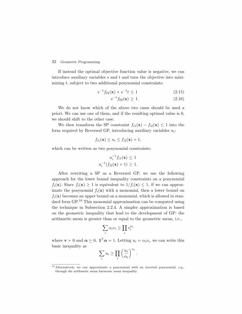
If instead the optimal objective function value is negative, we canintroduce auxiliary variables s and t and turn the objective into mini-mizing t, subject to two additional posynomial constraints:
s−1f01(x) + s−1t ≤ 1 (2.15)
s−1f02(x) ≥ 1. (2.16)
We do not know which of the above two cases should be used apriori. We can use one of them, and if the resulting optimal value is 0,we should shift to the other case.
We then transform the SP constraint fi1(x) − fi2(x) ≤ 1 into theform required by Reversed GP, introducing auxiliary variables ui:
fi1(x) ≤ ui ≤ fi2(x) + 1,
which can be written as two posynomial constraints:
u−1i fi1(x) ≤ 1
u−1i (fi2(x) + 1) ≥ 1.
After rewriting a SP as a Reversed GP, we use the followingapproach for the lower bound inequality constraints on a posynomialfi(x). Since fi(x) ≥ 1 is equivalent to 1/fi(x) ≤ 1, if we can approx-imate the posynomial fi(x) with a monomial, then a lower bound onfi(x) becomes an upper bound on a monomial, which is allowed in stan-dard form GP.10 This monomial approximation can be computed usingthe technique in Subsection 2.2.4. A simpler approximation is basedon the geometric inequality that lead to the development of GP: thearithmetic mean is greater than or equal to the geometric mean, i.e.,∑
i
αivi ≥∏i
vαii
where v 0 and α � 0, 1T α = 1. Letting ui = αivi, we can write thisbasic inequality as ∑
i
ui ≥∏i
(ui
αi
)αi
.
10 Alternatively, we can approximate a posynomial with an inverted posynomial, e.g.,through the arithmetic mean harmonic mean inequality.

2.2. Extensions 33
Let {ui(x)} be the monomial terms in a posynomial f(x) =∑
i ui(x). Alower bound inequality on posynomial f(x) can now be approximatedby an upper bound inequality on the following monomial:
∏i
(ui(x)αi
)−αi
.
This approximation is in the conservative direction because the orig-inal constraint is now tightened. There are many choices of α. Onepossibility is to let
αi(x) = ui(x)/f(x), ∀i,
which obviously satisfies the condition that α 0 and 1T α = 1. Givenan α for each lower bound posynomial inequality, a standard form GPcan be obtained based on the above geometric mean approximation ofa Reversed GP.
Notice that what is important is to have a monomial approximationof a posynomial. However, the geometric mean approximation and theabove choice of α may not lead to the best approximation in the senseof minimizing the approximation error or facilitating the computationof a global optimizer of SP.
An iterative procedure can now be used to solve the geometric meanapproximation of a Reversed GP. Start with any feasible xk and com-pute α(xk). Then solve the resulting standard form GP to obtain xk+1.If it is feasible in the original constraints of Reversed GP and makesthe approximation tight for (2.13,2.14,2.15,2.16), then stop. Otherwisecompute α(xk+1) and repeat the iterations of solving a GP based onthe geometric mean approximation using α(xk+1).
Approach 4: Complementary GP. The fourth approach to solveSP is similar to the third approach. It first converts a SP into a Com-plementary GP, which allows upper bound constraints on the ratiobetween two posynomials, and then applies a monomial approximationiteratively [10, 51]. This is called the condensation technique, which isan instance of the cutting-plane method for nonlinear programming.
The conversion from a SP into a Complementary GP is trivial. Aninequality in SP of the following form
fi1(x) − fi2(x) ≤ 1,

34 Geometric Programming
where fi1, fi2 are posynomials, is clearly equivalent to
fi1(x)1 + fi2(x)
≤ 1.
Now we have two choices to make the monomial approximation.One is to approximate the denominator 1+fi2(x) with a monomial butleave the numerator fi1(x) as a posynomial. This is called the (single)condensation method, and results in a GP approximation of a SP. Aniterative procedure can again be carried out: given a feasible xk, fromwhich a monomial approximations using α(xk) can be made and a GPformed, from which an optimizer can be computed and used as xk+1,the starting point for the next iteration. This sequence of computationof x may converge to x∗, a global optimizer of the original SP, but mayalso converge to a local optimum.
Another choice is to make the monomial approximation for both thedenominator posynomial 1 + fi2(x) and numerator posynomial fi2(x).That turns all the constraints into monomials, and after the log trans-formation, approximate SP as a LP. This is called the double conden-sation method, and a similar iterative procedure can be carried outas in the last paragraph. A key difference from the (single) condensa-tion method is that this LP approximation always generate solutionsthat are infeasible in the original SP. Therefore at the kth step ofthe iteration, the most violated constraint is condensed at xk, i.e., themonomial approximation is applied to this constraint inequality usingα(xk). The resulting new constraint is added to the LP approximationfor the (k + 1)th step of the iteration. The solution x∗ at which allconstraints in the original SP are satisfied is an optimum of the SP.
This iterative procedure of condensation uses a sequence of GPrelaxations for a wide class of nonlinear non-convex optimizationproblems. Compared to the recently developed algebraic sum-of-squares method using SDP relaxations [102, 101, 106] for constrainedpolynomial minimization (which becomes a special case of SP whenthe variables are restricted to the positive quadrant), this GP relax-ation method still lacks a theoretical foundation that guarantees itsperformance.
We conclude the quick tutorial on GP extensions in this subsec-tion with the following comment. As evidenced through the exam-

2.3. Algorithms 35
ples in Subsection 2.2.3 and this subsection, GP, with all these exten-sions, in fact covers a surprisingly wide range of nonlinear (convex ornon-convex) problems that may not even resemble a GP in standardform (2.1) or in convex form (2.3). Indeed, it is known [103] that anyoptimization where the feasible set is the intersection of the domainof objective and constraint functions and a cone can be turned intoa (most generalized version of) GP. Different cones lead to differentforms of GP in this most generalized sense, and different algebraicdescriptions of the cones lead to different separability structures of theresulting GP.
2.3 Algorithms
2.3.1 Numerical methods for GP
During the 1960s and 1970s, a variety of numerical methods were pro-posed for GP, ranging from the original one by Duffin, Peterson, andZener to ellipsoid methods. Some of them are based on primal GP whileothers on dual GP, some start with standard form while others convexform. Lists of representative GP problems for comparison of numericalmethods and performance evaluation of some solution packages werepublished as well [6, 47].
A measure of how difficult is a GP was proposed in [52]. Thedegree of difficulty of a GP is the difference between the total num-ber of monomial terms in the objective and constraints, and one plusthe number of variables. When the degree of difficulty is zero, solv-ing GP is equivalent to solving a system of linear equations. Modernnumerical methods seem to perform well independent of the degree ofdifficulty.
There are at least two major approaches to solve a GP using modernconvex optimization techniques. One is the interior-point method as in[97], and the other is an infeasible algorithm as in [78]. User-friendlysoftwares for GP are available on the Internet, such as the MOSEKpackage [129].
The standard barrier-based interior-point method for convex opti-mization can be applied to GP in a straightforward way, with a worst-case polynomial-time complexity and very efficient performance that

36 Geometric Programming
scales gracefully with problem size in practice. Consider the followingGP in convex form with m inequality constraints:
minimize f0(x) = log∑K0
k=1 exp(aT0kx + b0k)
subject to fi(x) = log∑Ki
k=1 exp(aTikx + bik) ≤ 0, i = 1, . . . , m
variables x.
The basic idea of the barrier-method is to solve a sequence ofunconstrained problems that absorb the constraints into a newobjective function, which is a weighted sum of the original objectivefunction and a barrier function φ of the constraints. As the weight t
on the original objective function becomes larger, the unconstrainedproblem becomes a tighter approximation of the original problem.
Barrier-method algorithm for GP [21]:Given a strictly feasible point x, which can be obtained either byverifying a given x to be strictly feasible or by solving a feasibilityGP problem, and t := t(0) > 0, µ > 1, and error tolerance ε > 0.Repeat(1) Centering step: compute x∗(t) by minimizing tf0(x) + φ(x)
starting at x. This is an unconstrained, smooth, convex min-imization that can be readily carried out by a variety of iter-ative methods, such as gradient descent method or Newton’smethod.
(2) Update: x := x∗(t).(3) Stopping criterion: Quit if m
t ≤ ε.(4) Increase t: t := µt.
If a log barrier function φ is used in item (1), we have
φ(x) = −m∑
i=1
log
− log
Ki∑k=1
exp(aTikx + bik)
.
A concise discussion on computational complexity and parame-ter choices for the above algorithm can be found in [21].
We now turn to a more complicated infeasible algorithm follow-ing Kortanek, Xu, and Ye [78], which solves both the primal anddual GP simultaneously, starting with convex form, and is reported

2.3. Algorithms 37
to produce very competitive numerical efficiency for a wide rangeof GPs. The basic technique is to apply Newton’s method to theperturbed Karush–Kuhn–Tucker (KKT) system with the help ofpredictor-corrector, coupled with effective techniques for choosingiterate directions and step lengths. Special structures of the Hes-sian of convex form GP is utilized in sparse matrix factorizations toaccelerate the computation.
The infeasible primal-dual method generates subfeasible solu-tions whose primal and dual objective function values converge tothe respective primal and dual optimal values. It is applied to thedual GP and its Wolfe dual problem. From Subsection 2.1.2, weknow that the dual of a GP with n variables, (m − 1) monomialterms, and p inequality posynomial constraints, can be written asthe following linearly constrained convex optimization:
minimize f(x)subject to Ax = b
x � 0variables x
where constant matrix A ∈ Rm×n and constant vector b ∈ Rm.11
The classical Wolfe dual problem to the above dual GP can bewritten as:
maximize bTy − xT ∇f(x) + f(x)subject to ATy − ∇f(x) + z = 0
where x ∈ Rn++ are the primal variable, and (y ∈ Rm, z ∈ Rn
+) arethe dual variables.
The primal feasibility, dual feasibility, and complementarity fea-sibility residuals are respectively defined by:
rP (x) = b − Ax
rD(x,y, z) = ∇f(x) − ATy − z
µ(x, z) =xTzn
.
11 Note that A in this subsection does not denote the exponent constant matrix used else-where in the survey. It represents the linear constraints in dual GP. The constant vectorb is simply an n + 1-dimensional vector with the first entry being 1 and the rest 0.

38 Geometric Programming
The duality gap is xT ∇f(x) − bTy. Let X = diag(x) and Z =diag(z).
Infeasible primal-dual algorithm for GP and dual GP [78]:Given the dual objective function f(x) and constants (A,b).Initialize y0,x0 � 0, z0 � 0.
(1) Compute the Hessian H = ∇2f(x).(2) Call Prediction Step Routine to compute γ ∈ [0, 1] and
η ∈ [0, 1].(3) Solve the following system of linear equation for (δy, δx, δz):
0 A 0AT −H I0 Z X
δy
δx
δz
=
ηrP
ηrD
γµ1 − Xz
. (2.17)
(4) Call Step Length Routine to compute α.(5) Update primal-dual solution:
y = y + αδy
x = x + αδx
z = z + αδz.
(6) Call Dual Slack Reset Routine to reset z.(7) Call Stopping Criterion Routine to determine if the iter-
ations can be stopped.
Prediction Step Routine
• Let η = 1 and γ = 0. Solve (2.17).• Compute α = min (maxj {−xj/δx,j : δx,j < 0} ,
(maxj {−zj/δz,j : δz,j < 0}).• Compute γ = 1
2µn(x + αδx)T (z + αδz) and η = 1 − γ.
Step Length Routine
• Compute αR = min (maxj {−xj/δx,j : δx,j < 0} ,(maxj {−zj/δz,j : δz,j < 0}).

2.3. Algorithms 39
• Choose αN such that (x(αN ),y(αN ), z(αN )) (updatedaccording to Step (5) in the algorithm) satisfy:
‖Xz‖ ≥ σµ
‖Xz − µ1‖ ≤ βµ
where σ ∈ (0, 1) and β > 0 are constant parameters.• Choose αC such that (x(αC),y(αC), z(αC)) (updated
according to Step (5) in the algorithm) satisfy:
θPx(αC)Tz(αC) ≥ ‖rP ‖θDx(αC)Tz(αC) ≥ ‖rD‖
x(αC)Tz(αC) ≤ θCxTz
where θP , θD, θC > 0 are constant parameters.• Choose the step length as:
α = min{θ1αR, αN , αC}where θ1 ∈ (0, 1) is a safety factor.
Dual Slack Reset Routine
• Let σ = ∇f(x) − ATy.• For each i, if σi ≥ 0, then
zi =
σi, σi ∈ (zi/θ2, ziθ2)zi/θ2, σi ≤ zi/θ2
ziθ2, σi ≥ ziθ2
where θ2 > 0 is a constant parameter.
Stopping Criterion RoutineIf the following inequalities are satisfied, then stop the algorithm,otherwise, return to Step (1).
‖rP ‖1
1 + ‖x‖1< εP
‖rD‖1
1 + ‖z‖1< εD
xTz1 + ‖x‖1 + ‖z‖1
< εC
where εP , εD, εC are constant parameters.

40 Geometric Programming
The following values for constant parameters are recommendedin [78]:
• x0 = 1,y0 = 0, z0 = 1 as initial points.• σ = 10−8, β = 103, θP = 100 ‖r0
P ‖x0T z0 , θD = 104 ‖r0
P ‖x0T z0 , θC = 2
and θ1 = 0.9995 in Step Length Routine.• θ2 = 100 in Dual Slack Reset Routine.• εP = 10−8, εD = 10−8, εC = 10−12 in Stopping Criterion
Routine.
The most computationally intensive step in the algorithm is Step3 that solves a KKT system of linear equations, which can be simpli-fied as:(
−X−1Z − H AT
A 0
)(δx
δy
)=
(ηrD − X−1(γµ1 − Xz)
ηrP
).
Solving this linear system of equations can be accomplished by com-puting matrix K = A(X−1Z + H)AT . Because the Hessian H of dualGP is a block diagonal matrix with sparse blocks, and X−1Z + H hasthe same block diagonal structure with blocks Hk, matrix K can bewritten as
K =p∑
j=0
AjHjATj .
This decomposition greatly simplifies the numerical solution in Step(3) of the algorithm.
As reported in [78], this infeasible primal-dual algorithm is testedon 19 typical GP problems, including 3 that are generally viewed asthe most difficult, and the computational time is orders of magnitudefaster than the earlier methods.
2.3.2 Numerical methods for robust GP
In the area of robust optimization [11, 13, 63, 62], we solve an opti-mization problem by taking into account possible perturbations of theproblem parameters. A series of results on robust conic optimization,especially robust SDP and robust SOCP, have been obtained over thelast decade in addition to the classical robust LP results.
2.3. Algorithms 41
Recall that the constant parameters of a GP can be written asa set of exponent constant matrices {Ai} and a set of multiplicativeconstant vectors {bi}, i = 0, 1, . . . , m, where A0 and b0 correspond tothe objective posynomial, and the other Ai ∈ RKi×n and bi ∈ RKi
correspond to the m inequality constraints. In the worst-case robustGP formulation, each log-sum-exp function in the original GP need tobe replaced by the supremum of the set of log-sum-exp functions whoseparameters Ai and bi belong to the image of a set U in RL under anaffine mapping:
(Ai, bi) =
A0
i +L∑
j=1
ujAji ,b
0i +
L∑j=1
ujbji
, ∀u ∈ U
where Aji ,b
ji , j = 0, 1, . . . , L are given matrices and vectors describing
the uncertainty.In some cases, a robust GP can be formulated as a GP [11]. A
method to approximately solve a general robust GP has recently beenproposed in [67]. This numerical method for robust GP is based on theidea of approximating a posynomial with a piecewise linear function.
First a general robust GP is reduced to a two-term robust GP, whereeach posynomial has only two monomial terms. This reduction can beconducted in a numerically efficient way and decreases the computa-tional load of approximating a general multi-variate function. After thelog transformation, a two-term posynomial is turned into a two-termlog-sum-exp function:
log(exp(y1) + exp(y2)),
which is then approximated by a r-term piecewise linear convexfunction:
maxi=1,2,...,r
{cTi y + di}
where ci, di are constants. Replacing the log-sum-exp functions withthe best piecewise linear approximations, a robust GP is turned into arobust LP formulation.
When the set of uncertainty is polyhedral:
U = {u ∈ RL|Du � d}

42 Geometric Programming
where (D,d) describe the finite number of hyperplanes that define theuncertainly set, or ellipsoidal:
U = {u + Dρ|ρ ∈ RL, ‖ρ‖2 ≤ 1}
where D describes the possible variations of GP parameters, the result-ing robust LP becomes another LP or a Second Order Cone Program,respectively. Thus efficiently solvable as a standard convex optimizationproblem.
As the piecewise linear approximation becomes tighter, the approx-imate robust GP (in the form of a robust LP) approaches the exact for-mulation of the original robust GP. However, to maintain a given levelof approximation accuracy, the size of robust LP that approximates therobust GP grows exponentially with the number of monomial terms.
2.3.3 Distributed algorithms
We present a systematic theory of distributed algorithms for GP, whichis particularly useful for networking applications. While efficient androbust algorithms have been extensively studied for centralized solutionof GP, distributed solutions for GP have not been fully explored before.This subsection shows how special structures of GP can be utilized fordistributed computation of a globally optimal solution.
Based on the sparsity pattern of the exponent matrix A, it issometimes natural to decompose a GP into several small decoupledGPs. This is a straightforward application of the standard decomposi-tion method for convex optimization with decoupled constraints (e.g.,[18, 103]), and will not be further discussed here.
Special cases. We first present three special cases of GP wheresimple distributed algorithms have been found, by dual decomposition,or by linear system evolution using the Perron–Frobenius theory ofpositive matrix, or by message-passing-based iteration of gradient algo-rithms. These special cases include linearly constrained maximizationof a monomial, unconstrained minimization of a product of posynomi-als, and feasibility problem with a special structure of the exponentconstant matrix A and multiplicative constant vector d. These casesare motivated by networking problems to be covered in Section 3.

2.3. Algorithms 43
Case 1. Consider the following linearly constrained monomial max-imization:
maximize∏
j xaj
j
subject to∑
j Rijxbj
j ≤ 1, i = 1, . . . , m
variables x
where {Rij}, {aj} are non-negative constants, and {bj} are real con-stants. It is important to note that in this case the exponent constants{bj} do not depend on the constraint index i. A distributed algorithmfor this class of GP is described in Subsection 3.4.1 in the applicationof TCP Vegas congestion control.
Case 2. Consider the following GP feasibility problem: find an xsuch that the following posynomial inequalities are satisfied:∑
j �=i
Aijxjx−1i ≤ ρ, i = 1, . . . , m
where Aij are positive constants. This is a model of a wireless powercontrol problem. Define a matrix A where the off-diagonal entries areAij and diagonal entries zero. It is known [60] that if 1/ρ is smaller thanthe Perron–Frobenius eigenvalue λmax(A) of A, the feasibility problemhas a solution, and the following simple, iterative update of x convergesgeometrically to a feasible solution over iterations indexed by t:
x(t + 1) = Ax(t).
This update can be carried out distributively. Each xi is updated tomake the ith posynomial constraint be satisfied with equality, assumingthat the other {xj , j �= i} do not change.
Case 3. Consider the following unconstrained minimization of thecomposition of a monomial and a posynomial of x:
minimize∏i
∑
j �=i
Aijxjx−1i
ai
where Aij , ai are positive constants. In an application to jointly optimalcongestion and power control in Subsection 3.4.2, a gradient methodto solve this GP will be turned into a distributed algorithm with the

44 Geometric Programming
help of message passing among the network elements each controllingan xi.
General approach. Based on recent results in [37], we show that,by allowing message passing, a dual decomposition technique can beused to distributively solve any standard form GP. Here, each termor each constraint equation has a corresponding interpretation of anetwork element (end user or intermediate nodes). This method can beused to distributively solve all the GP problems formulated in Section 3for various applications in information theory, coding, signal processing,and networking, especially for power control problems. It can also beused to decouple any convex optimization with additive objective andconstraint functions:
minimize∑
s fs(x)subject to
∑j hij(x) ≤ 0, ∀i
where fs and hij are all convex functions.Objective and constraint functions in GP are additive, with coup-
ling of variables across the monomial terms. Had there been no coup-ling, the additive structure leads to an easy parallel computation. Thekey approach to tackle the coupling problem is to introduce auxil-iary variables and additional equality constraints, thus transferringthe coupling in the objective function to coupling in the constraints,which can be decoupled by dual decomposition and solved by intro-ducing ‘consistency pricing’. Updates of ‘consistency price’ can be con-ducted via local communication channels among the variables thatare coupled with each other. This method is illustrated through anunconstrained GP, and extensions to problems with constraints arestraightforward.
Suppose we have the following unconstrained standard form GP inx 0:
minimize∑
i fi(xi, {xj}j∈I(i)) (2.18)
where xi denotes the local variable of the ith user, I(i) denotes theset of coupled variables from other users, and {fi} are posynomials.Making a change of variable yi = log xi,∀i, in the original problem, weobtain the following convex optimization problem in y:
minimize∑
i fi(eyi , {eyj}j∈I(i)).

2.3. Algorithms 45
We now rewrite the problem by introducing auxiliary variables{yij} for the coupled arguments, and additional equality constraintsto enforce consistency between the original variables and the auxiliaryvariables:
minimize∑
i fi(eyi , {eyij}j∈I(i))subject to yij = yj , ∀j ∈ I(i),∀i
variables {yi}, {yij}.
(2.19)
Each ith user controls the local variables (yi, {yij}j∈I(i)). Next, theLagrangian of (2.19) is formed as
L({yi}, {yij}, {γij}) =∑
i
fi(eyi , {eyij}j∈I(i)) +∑
i
∑j∈I(i)
γij(yj − yij)
=∑
i
Li(yi, {yij}, {γij})
where each partial Lagrangian term is
Li(yi, {yij}, {γij}) = fi(eyi , {eyij}j∈I(i)) +( ∑
j:i∈I(j)
γji
)yi −
∑j∈I(i)
γijyij .
(2.20)The minimization of the Lagrangian with respect to the primal vari-ables ({yi}, {yij}) can be done simultaneously, in a parallel fashion, byeach user. In the more general case where the original problem (2.18)is constrained, the additional constraints can be included in the mini-mization of each Li.
The following master dual problem has to be solved to obtain theoptimal dual variables or consistency prices {γij}:
maximize{γij} g({γij}) (2.21)
whereg({γij}) =
∑i
minyi,{yij}
Li(yi, {yij}, {γij}).
Note that the transformed primal problem (2.19) is convex with zeroduality gap. Hence the Lagrange dual problem indeed solves the originalstandard GP problem. A simple way to solve the maximization in (2.21)is with the following update for the consistency prices:
γij(t + 1) = γij(t) + α(t)(yj(t) − yij(t)). (2.22)

46 Geometric Programming
Appropriate choice of the stepsize α(t) > 0 leads to convergence of thedual algorithm [16].
Summarizing, we have the followingDistributed Algorithm for Unconstrained GP [37]:The ith user does the following:
(1) Minimize Li in (2.20) involving only local variables, uponreceiving the updated dual variables {γji, j : i ∈ I(j)} (notethat {γij , j ∈ I(i)} are local dual variables).
(2) Update the local consistency prices {γij , j ∈ I(i)} with(2.22).
The amount of message passing overhead in the above distributedalgorithm can be substantially reduced using the structures of the cou-pling variables. The general approach of distributed GP solution andspecific overhead reduction techniques will be illustrated in Subsection3.3.1 through distributed GP-based power control.

3Applications in Communication Systems
3.1 Information Theory
Materials in this subsection are in part based on recent publications[30, 33, 82, 84], and some problems have been studied in the 1980s and1990s [120, 121, 122].
We are concerned with two information theoretic limits on datatransmission and compression in this section, focusing on the single-user, discrete memoryless system models: channel capacity as the max-imum transmission rate so that the decoding error probability vanishesas the codeword becomes long, and rate distortion function as the min-imum rate required to describe a source so that the decoder’s averagedistortion is no larger than a threshold distortion value.
We will show that the Lagrange dual problems of channel capac-ity and rate distortion can be simplified into GPs.1 The struc-tures of these GPs allow us to efficiently generate upper boundson channel capacity and lower bounds on rate distortion by solving
1 The Lagrange dual problem of a given primal problem may be represented in severaldifferent but equivalent ways. It is important to reduce it the most illuminating and usefulform.
47

48 Applications in Communication Systems
systems of linear inequalities (Subsections 3.1.1 and 3.1.2), to charac-terize Shannon duality between transmission and compression (Sub-section 3.1.3), and to interpret channel capacity and rate distor-tion problems as free energy optimization in statistical physics(Subsection 4.1.1).
3.1.1 Channel capacity
First consider the problem of data transmission over a discrete mem-oryless channel with input X ∈ X = {1, 2, . . . , N}, output Y ∈Y = {1, 2, . . . , M}, and channel law Pij = Prob{Y = j|X = i}, i =1, 2, . . . , N, j = 1, 2, . . . , M . The channel law forms a channel matrixP ∈ RN×M , where the (i, j) entry of P is Pij ≥ 0 with P1 =1. A distribution p ∈ RN×1 on the input, together with a givenchannel matrix P, induces a distribution q ∈ RM×1 on the out-put by q = PTp, and a joint distribution Q ∈ RN×M on theinput output pair by Qij = piPij . We also associate with each inputalphabet symbol i an input cost si ≥ 0, forming a cost vectors ∈ RN×1.
It is a key result in information theory (e.g., [40, 94]) that the capac-ity C(S) of a discrete memoryless channel, under the input cost con-straint Ep[s] = pT s ≤ S for a given total cost S ≥ 0, is
C(S) = maxp:pT s≤S
I(X; Y ) (3.1)
where the mutual information I between input X and output Y isdefined as
I(X; Y ) =N∑
i=1
M∑j=1
Qij logQij
piqj= H(Y )−H(Y |X) = −
M∑j=1
qj log qj−pT r
where r ∈ RN×1 and ri = −∑Mj=1 Pij log Pij is the conditional entropy
of Y given X = i.

3.1. Information Theory 49
Therefore we view channel capacity as the optimal objective value ofthe following maximization problem, referred to as the channel capacityproblem with input cost:2
maximize −pT r − ∑Mj=1 qj log qj
subject to PTp = qpT s ≤ S
1Tp = 1p � 0
variables p,q.
(3.2)
The constant parameters are P, the channel matrix, and ri =−∑M
j=1 Pij log Pij , ∀i. In the special case of no input cost constraint,the channel capacity problem becomes:
maximize −pT r − ∑Mj=1 qj log qj
subject to PTp = q1Tp = 1p � 0
variables p,q.
(3.3)
If we substituted q = PTp in the objective function of (3.2), wewould later find that the Lagrange dual problem can only be implicitlyexpressed through the solution of a system of linear equations. Keepingtwo sets of optimization variables, p and q, and introducing the equal-ity constraint PTp = q in the primal problem is a key step to derivean explicit and simple Lagrange dual problem of the channel capacityproblem.
Theorem 3.1. The Lagrange dual of the channel capacity problemwith input cost (3.2) is the following GP (in convex form):
minimize log∑M
j=1 exp(αj + γS)subject to Pα + γs � −r
γ ≥ 0variables α, γ
(3.4)
The constant parameters are P, s and S.
2 Showing that channel capacity can be obtained as a maximized mutual informationrequires achievability and converse proofs, which are not discussed in this subsection.

50 Applications in Communication Systems
An equivalent version of the Lagrange dual problem is the followingGP (in standard form):
minimize wS ∑Mj=1 zj
subject to wsi∏M
j=1 zPij
j ≥ e−H(P(i)), i = 1, 2, . . . , N
w ≥ 1, zj ≥ 0, j = 1, 2, . . . , M
variables z, w
(3.5)
where P(i) is the ith row of P.Lagrange duality between problems (3.2) and (3.4) means the
following:
• Weak duality. Any feasible (α, γ) of the Lagrange dual prob-lem (3.4) produces an upper bound on channel capacity withinput cost: log
∑Mj=1 exp(αj + γS) ≥ C(S).
• Strong duality. The optimal value of the Lagrange dual prob-lem (3.4) is C(S).
The proof can be found in Appendix B.1.
Corollary 3.1. The Lagrange dual of the channel capacity problemwithout input cost (3.3) is the following GP (in convex form)
minimize log∑M
j=1 eαj
subject to Pα � −rvariables α.
(3.6)
The constant parameters are P.An equivalent version of the Lagrange dual problem is the following
GP (in standard form):
minimize∑M
j=1 zj
subject to∏M
j=1 zPij
j ≥ e−H(P(i)), i = 1, 2, . . . , N
zj ≥ 0, j = 1, 2, . . . , M
variables z.
(3.7)
The constant parameters are P, and P(i) is the ith row of P.

3.1. Information Theory 51
Lagrange duality between problems (3.3) and (3.6) means thefollowing:
• Weak duality. log(∑M
j=1 eαj
)≥ C, for all α that satisfy Pα+
r � 0.• Strong duality. log
(∑Mj=1 eα∗
j
)= C, where α∗ are the opti-
mal dual variables.
We can also prove the weak duality result in Corollary 3.1 on channelcapacity upper bound in a simple way without using the machinery ofLagrange duality. This short proof is shown in Appendix B.2.
Note that the Lagrange dual (3.7) of the channel capacity problemis a simple GP with a linear objective function and only monomialinequality constraints. Also, dual problem (3.5) is a generalized versionof dual problem (3.7), weighing the objective function by wS and eachconstraint by wsi , where w is the Lagrange multiplier associated withthe input cost constraint. If the costs for all alphabet symbols are 0,we can analytically minimize the objective function over w by simplyletting w = 0, indeed recovering the dual problem (3.7) for channelswithout the input cost constraint.
We can interpret the Lagrange dual problem (3.6) as follows. LetΛ : {1, . . . , M} → R be a real-valued function on the output space,with Λ(j) = αj . We can think of the variables α as parameteriz-ing all real-valued functions on the output space, so the dual prob-lem is one over all real-valued functions on the output space. Since(Pα)i =
∑Mj=1 αjPij = E(Λ|X = i), the inequality constraint in the
dual states that for each i, E(Λ|X = i) exceeds −ri = −H(Y |X = i).Since maxj αj ≤ log
(∑Mj=1 eαj
)≤ maxj αj + log M , the objective
function in the dual is a smooth approximation of the maximum func-tion. Thus, the Lagrange dual problem asks us to consider all real-valued functions Λ on the output space, for which E(Λ|X = i) exceeds−H(Y |X = i) for each i. Among all such Λ, we are to find the one thatminimizes a smoothed approximation of the maximum value of Λ.
Suppose we have solved the GP dual3 (3.4) of channel capacity.By strong duality, we obtain C(S). We can also recover the optimal
3 GP dual refers to the Lagrange dual problem (of some primal problem) that is a GP, notto be confused with the Lagrange dual problem of GP.

52 Applications in Communication Systems
primal variables, i.e., the capacity achieving input distribution, fromthe optimal dual variables. For example, we can recover a least-normcapacity-achieving input distribution for a channel as follows. First, theoptimal output distribution q∗ can be recovered from the optimal dualvariable α∗:
q∗j = exp
(α∗
j − C)
, j = 1, 2, . . . , M (3.8)
where C = log∑M
j=1 eα∗j , and the optimal input distribution p∗ is a
vector that satisfies the linear equations:
−pT r = C + e−C
M∑
j=1
α∗je
α∗j − C
M∑j=1
eα∗j
,
PTp = q∗,
1Tp = 1.
The primal and dual problems of C(S) can be simultaneously andefficiently solved through a primal-dual interior point algorithm [97,21], which scales smoothly for different channels and alphabet sizesand provides an alternative to the classical Blahut–Arimoto algorithm[3, 19]. Due to the structure and sparsity of the exponent constantmatrix A of the GP dual for channel capacity, standard GP algorithmslike the ones in Subsection 2.3.1 can be further accelerated.
Complementary slackness between (3.2) and (3.4) states that p∗i = 0
if ri + (Pα∗)i + γ∗si > 0 in the Lagrange dual of channel capacity.Therefore, from the optimal dual variables (α∗, γ∗), we immediatelyobtain the support of the capacity achieving input distribution as thefollowing set:
{i|ri + (Pα∗)i + γ∗si = 0}.
From the primal and dual problems of channel capacity, we obtainthe following optimality conditions. If there are λ and α satisfying thefollowing KKT conditions [21] for a given P:
λ � 0,
r + Pα � 0,

3.1. Information Theory 53
eαj∑Mj′=1 eαj′ +
N∑i=1
λiPij = 0, j = 1, 2, . . . , M,
λi(ri +M∑
j=1
Pijαj) = 0, i = 1, 2, . . . , N,
then the resulting log∑M
j=1 eαj is the channel capacity C.Because the inequality constraints in the dual problem (3.4) are
affine, it is easy to find a dual feasible α, and the resulting value ofthe dual objective function provides an easily-derived upper boundon channel capacity. Based on the sparsity pattern of a given channelmatrix, tight analytic bounds may also be obtained from an appropriateselection of dual variables.
As a simple example, it is easy to verify that αj = log maxi Pij , ∀j,
satisfy the dual constraints and give the following
Corollary 3.2. Channel capacity is upper bounded in terms of a max-imum likelihood receiver selecting argmaxi Pij for each output alphabetsymbol j:
C ≤ logM∑
j=1
maxi
Pij , (3.9)
which is tight if and only if the optimal output distribution q∗ is
q∗j =
maxi Pij∑Mk=1 maxi Pik
, j = 1, 2, . . . , M.
When there is an input cost constraint pT s ≤ S, the above upperbound becomes
C(S) ≤ logM∑
j=1
maxi
(e−siPij) + S (3.10)
where each maximum likelihood decision is modified by the cost vector s.
Of course, it is trivial to find a primal feasible point satisfying thelinear inequality constraints of the primal problem (3.3), which gives alower bound on channel capacity. This pair of bounds provides an esti-mate of C(S). Therefore, given a dual feasible variable, by generating
54 Applications in Communication Systems
the corresponding primal feasible variable, both an upper and a lowerbound on channel capacity are obtained. The worst case differencebetween the true value of channel capacity and the estimate basedon either bound is the gap between these two bounds. This is a com-putationally easy method to generate an estimate of channel capacitywith bounded error. For example, for channel capacity without inputcost, find any dual feasible α, from which we generate
qj =eαj∑M
k=1 eαk.
If there is a p such that PTp = q, then the estimated channel capacityC = log
∑Mj=1 eαj can only be Γ away from the true capacity C, where
Γ = pT r +∑M
j=1 αjeαj∑M
j=1 eαj.
There is a minmax Kullback–Leibler divergence (minmaxKL) char-acterization of discrete memoryless channel capacity with input costin [42]:
C(S) = minq
minγ≥0
maxi
[D(P(i)‖q) + γ(S − si)
](3.11)
where the minimization over q is over all possible output distributions.This characterization of C obviously leads to the following known
class of upper bounds on channel capacity: for any output distribution q,
C ≤ maxi
M∑j=1
Pij logPij
qj, (3.12)
which is shown in [42, 61], and has recently been used for simulatingfinite state channels in [124] and bounding the capacity of non-coherentmultiple antenna fading channels in [83].
Since the Lagrange dual (3.4) and minmaxKL (3.11) characteriza-tions both give C(S), they must be equivalent. This equivalence can alsobe established directly. Let the dual variables zj = eαj = βqj whereβ > 0 and q is any distribution. Then the dual constraints become∑M
j=1 Pij log Pij
qj−γsi ≤ log β, i = 1, 2, . . . , N . Since the case of C(S) =
0 is trivial, assume C(S) > 0. By complementary slackness, if at opti-mality all the dual constraints are satisfied with strict inequalities, then

3.1. Information Theory 55
the optimal Lagrange multipliers (readily seen to be the optimal inputdistribution) of this GP must all be zero, contradicting our assumption
that C(S) > 0. Therefore, maxi
[∑Mj=1 Pij log Pij
q∗j
− γ∗si
]= log β∗. By
the strong duality part of Theorem 3.1,
C(S) = logM∑
j=1
β∗q∗j + γ∗S = log β∗ + γ∗S
= maxi
M∑
j=1
Pij logPij
q∗j
− γ∗si
+ γ∗S.
Since at optimality, q∗ must correspond to the output distributioninduced by an optimal input distribution, restricting the minimizationof dual variables z to a scaled version of an output distribution incursno loss of generality. Thus the minmaxKL characterization (3.11) isrecovered.
The above argument shows that the GP Lagrange dual (3.4) gen-erates a broader class of upper bounds on C(S), including the class ofbounds from (3.12) as a special case. Specifically, the following bounds,readily extended from (3.12) and parameterized by output distributionsq and γ ≥ 0:
C(S) ≤ maxi
M∑
j=1
Pij logPij
qj− γsi
+ γS,
can be obtained from the GP dual by restricting the dual variables (z, γ)to be such that maxi
[∑Mj=1 Pij log Pij
zj− γsi
]= 0, and by restricting z
to be a scaled output distribution.For a memoryless channel with continuous alphabets, where the
channel is a family of conditional distributions P (y|x) and input costconstraint is
∫p(x)s(x)dx ≤ S, a derivation similar to the discrete case
shows that the Lagrange dual of the channel capacity problem is thefollowing continuous analog of GP:
minimize log∫
z(y)dy + γS
subject to∫
P (y|x) log z(y)P (y|x)dy + γs(x) ≥ 0, ∀x
z(y) ≥ 0,∀y, γ ≥ 0variables z(y), γ.
(3.13)

56 Applications in Communication Systems
Although, in general, the KKT optimality condition can be compli-cated in the infinite dimensional case, weak duality and the Lagrangedual problem (3.13) readily lead to the following class of bounds [83, 33]:for any distribution q(y) and γ ≥ 0,
C(S) ≤ maxx
[∫P (y|x) log
P (y|x)q(y)
dy − γs(x)]
+ γS.
3.1.2 Rate distortion
Consider the following information theoretic problem of data compres-sion. Assume a source that produces a sequence of i.i.d. random vari-ables X1, X2, . . . , Xn ∼ p, where the state space of Xi is a discretesource alphabet X with N alphabet symbols and p ∈ RN×1 is thesource distribution. The encoder describes the source sequence Xn byan index fn(xn) ∈ {1, 2, . . . , 2nR}, where xn is a realization of Xn.The decoder reconstructs Xn by an estimate Xn = gn(fn(Xn)) in afinite reconstruction alphabet X . Given a bounded distortion measured : X × X → R+, the distortion d(xn, xn) between sequences xn andxn is the average distortion of these two n letter blocks.
It is another key result in information theory that the rate distortionfunction R(D) of a discrete source can be evaluated as the minimummutual information I(X; X) between the source and the reconstructionunder the distortion constraint:
R(D) = minP:E[d(X,X)]≤D
I(X; X) (3.14)
where Pij = Prob{X = j|X = i}, i = 1, 2, . . . , N, j = 1, 2, . . . , M arethe reconstruction probabilities.
Writing out the minimization problem (3.14) explicitly, we have thefollowing rate distortion problem:
minimize∑N
i=1∑M
j=1 piPij log Pij∑k
Pkjpk
subject to∑N
i=1∑M
j=1 piPijdij ≤ D∑Mj=1 Pij = 1, i = 1, 2, . . . , N
Pij ≥ 0, i = 1, 2, . . . , N, j = 1, 2, . . . , M
variables P.
(3.15)

3.1. Information Theory 57
The constant parameters are the source distribution p, the distortionmeasures dij = d(X = i, X = j), and the distortion constraint D.
Theorem 3.2. The Lagrange dual of the rate distortion problem(3.15) is the following GP (in convex form):
maximize pT α − γD
subject to log∑N
i=1 exp(log pi + αi − γdij) ≤ 0,
j = 1, 2, . . . , M γ ≥ 0variables α, γ.
(3.16)
The constant parameters are p, dij and D.An equivalent version of the Lagrange dual problem is the following
GP (in standard form):
maximize w−D ∏Ni=1 zpi
i
subject to∑N
i=1 piziw−dij ≤ 1, j = 1, 2, . . . , M
w ≥ 1, zi ≥ 0, i = 1, 2, . . . , N
variables z, w.
(3.17)
Lagrange duality between problems (3.14) and (3.16) means thefollowing
• Weak duality. Any feasible (α, γ) of the Lagrange dual prob-lem (3.16) produce a lower bound on the rate distortionfunction:
pT α − γD ≤ R(D).
• Strong duality. The optimal value of the Lagrange dual prob-lem (3.16) is R(D).
In [14] Berger proved an equivalent formulation as (3.16). The proofin Appendix B.3 is simpler by directly using the Lagrange duality argu-ment.
The Lagrange dual (3.17) of the rate distortion problem (3.15) isa simple GP: maximizing a monomial over posynomial constraints, inthe form of maximizing a geometric mean
∏Ni=1 zpi
i weighted by w−D,under constraints on arithmetic means
∑Ni=1 pizi weighted by w−dij .

58 Applications in Communication Systems
A smaller shadow price w would reduce the objective value but alsoloosen each constraint, allowing larger dual variables zi and possibly ahigher objective value.
Similar to the case for channel capacity, we can now efficiently lowerbound the rate distortion function from the dual problem in the GPform. In particular, due to the structure of the constraints in (3.17),for any given w, finding a dual feasible z reduces to the easy task ofsolving a system of linear inequalities. For example, with the Hammingdistortion measure, it is easy to verify that αi = log
(1−Dpi
), ∀i, and
γ = log(
(1−D)(N−1)D
)satisfy the Lagrange dual constraints in (3.16),
and give the following lower bound:
R(D) ≥ H(X) − H0(D) − D log(N − 1) (3.18)
where H0(x) = −x log x − (1 − x) log(1 − x) is the binary entropyfunction.
Now consider guessing a random variable X based on another ran-dom variable X. If we replace D by the probability of estimation errorPe and use the fact that R(D) = min I(X; X) ≤ H(X) − H(X|X),then the lower bound (3.18) recovers Fano’s inequality:
H(X|X) ≤ H0(Pe) + Pe log(N − 1) (3.19)
that helps prove the converse theorem for channel capacity [40].The problem of rate distortion with state information [39, 130]
also has a Lagrange dual problem in the form of GP [33], and theLagrange duality bounding technique leads to a generalization of Fano’sinequality. The Lagrange dual problems for channel capacity and ratedistortion with generalized information measures were also derived in[120, 121].
3.1.3 Shannon duality
Lagrange duality is often loosely stated as follows. Given an optimiza-tion problem called the primal problem, the objective and constraintfunctions in the dual problem can be obtained from those in the primalproblem by some simple mappings of signs, variables, constant param-eters and mathematical operations. This ‘duality by mapping’ that

3.1. Information Theory 59
turns one optimization problem into its Lagrange dual is also foundin other duality relationships [90], such as that between controllabilityand observability. However, as can be easily verified, ‘duality by map-ping’ does not hold between the primal problems of channel capacity(3.2) and rate distortion (3.15). It turns out that their Lagrange dualproblems exhibit a precise ‘duality by mapping’. Due to strong dual-ity, this induces a ‘duality by mapping’ between the primal problemsthrough the GP duals, as shown in Figure 3.1. Note that Lagrangeduality is different from Shannon duality. Indeed, while channel capac-ity and rate distortion are ‘somewhat dual’ as commented by Shannon[114], their Lagrange dual problems are both GPs.
Shannon
Lagrange
C(S) R(D)
Dual C(S) Dual R(D)
Fig. 3.1 Shannon duality characterized through the Lagrange dual problems of channelcapacity and rate distortion.
We first summarize two versions of the Lagrange dual problems forC(S) and R(D) in Table 3.1, where the GP dual problems in standardform better illustrate the ‘duality by mapping’ relationships. The objec-tive functions, constraint functions, variables, and constant parametersin the Lagrange dual problems of C(S) and R(D) can be obtained fromone another through the following simple mappings:
Shannon Duality Correspondence
Channel capacity C(S) Rate distortion R(D)
monomial ↔ posynomial
posynomial ↔ monomial

60 Applications in Communication Systems
Lagr
ange
Dua
lof
Cha
nnel
Cap
acity
Lagr
ange
Dua
lof
Rat
eD
isto
rtio
n
Con
vex
Form
min
imiz
elo
g∑ M j
=1eα
j+
γS
subje
ctto
∑ M j=
1P
ij(α
j−
log
Pij
)+
γs i
≥0,
γ≥
0,va
riab
les:
αj,γ
cons
tant
s:ch
anne
lP
ij,
cost
s i,S
max
imiz
epα
−γD
subje
ctto
log∑ N i=
1el
og
pi+
αi−
γd
ij
≤0
γ≥
0va
riab
les:
αi,γ
cons
tant
s:so
urce
pi,
dist
orti
ond
ij,D
Stan
dard
Form
min
imiz
ew
S∑ M j
=1z j
subje
ctto
∏ M j=
1eH
(P(i
)) w
siz
Pij
j≥
1,w
≥1,
z j≥
0va
riab
les:
z j,w
cons
tant
s:ch
anne
lP
ij,
cost
s i,S
max
imiz
ew
−D∏ N i=
1z
pi
i
subje
ctto
∑ ip
iz i
w−
dij
≤1,
w≥
1,z i
≥0
vari
able
s:z i
,wco
nsta
nts:
sour
cep
i,
dist
orti
ond
ij,D
Tab
le3.
1Lag
rang
edu
alpr
oble
ms
ofch
anne
lca
paci
tyw
ith
inpu
tco
stan
dra
tedi
stor
tion
.
3.1. Information Theory 61
minimization ↔ maximization
≥ constraints ↔ ≤ constraints
j(receiver side index) ↔ i(sender side index)
i(sender side index) ↔ j(receiver side index)
wS ↔ w−D
wsi ↔ w−dij
zj ↔ zpii
zPij
j ↔ zi
H(P(i)) ↔ − log1pi
Lagrange duality gives a detailed analysis of the structures inShannon duality:
• It resolves the apparent asymmetry between maximizing overa vector p in the channel capacity problem and minimiz-ing over a matrix P in the rate distortion problem. In theLagrange dual of C(S), there are as many optimization vari-ables as output alphabet symbols, plus a shadow price forthe cost constraint. In the Lagrange dual of R(D), there areas many optimization variables as input alphabet symbols,plus a shadow price for the distortion constraint.
• It answers the following question: since a vector p (the sourcedistribution) is given in the rate distortion problem, and amatrix P (the channel matrix) is given in the channel capac-ity problem, what is the proper analog of pi (the ith entryin p) in the channel capacity problem? The last pair in theShannon duality correspondence shows that the proper ana-log of log 1
piin rate distortion is H(P(i)) in channel capacity:
log 1pi
is the number of bits to describe an alphabet symbolwith probability pi in the Shannon code for lossless compres-sion, and H(P(i)) is the number of bits needed to describewithout loss a source whose distribution follows the ith rowof channel matrix. This correspondence can be interpreted inthe context of universal source coding, where each row P(i)

62 Applications in Communication Systems
of the channel matrix represents a possible distribution of asource.
• It confirms Shannon’s remark in [114] on introducing inputcosts to enhance duality. From the Lagrange dual problems instandard form GP, it is easy to see that input costs s and costconstraint S in the C(S) dual problem are complementaryto distortion measures dij and distortion constraint D in theR(D) dual problem.
• The dual variable w ≥ 1 can be interpreted as the shadowprice associated with the input cost constraint S and with thereconstruction distortion constraint D, respectively. Fromlocal sensitivity analysis [21], the optimal −w∗ tells usapproximately how much increase in capacity C(S) or reduc-tion in rate R(D) would result if the cost or distortionconstraint can be relaxed by a small amount. From globalsensitivity analysis [21], if w∗ is large, then tightening thecost or distortion constraint will greatly decrease capacity(in the channel capacity problem) or increase rate (in therate distortion problem). If w∗ is small, then loosening thecost or distortion constraint will not significantly increasecapacity or decrease rate.
In addition to the above Lagrange duality based characteriza-tion, Shannon duality has also been characterized for single-userand multiple-user models through functional duality and operationalduality.4
3.1.4 Error exponent
Channel capacity is the x-intercept of an exponential decay curveof the decoding error probability: when the transmission rate R isbelow capacity C, the average decoding error probability P
(N)e (R)
decreases exponentially as the codebook length N tends to infinity, and
4 The functional duality [105] and Lagrange duality approach together imply that solving aGP in the form of (3.4) induces a set of problem parameters for another GP in the formof (3.16), whose optimal value equals that of the first GP.

3.1. Information Theory 63
the corresponding exponent is called the reliability function E(R) =limN→∞ − 1
N log P(N)e (R).
Reliability function is usually approximated by the following ran-dom coding upper bound on error probability [61]:
P (N)e (R) ≤ exp(−NEr(R)). (3.20)
The random coding exponent Er(R) is the maximized value of theobjective function in the following optimization problem:
maximize E0(ρ,p) − ρR
subject to 1Tp = 1p � 0ρ ∈ [0, 1]
variables p, ρ
(3.21)
where
E0(ρ,p) = − log∑j
(∑i
pi (Pij)1
1+ρ
)1+ρ
. (3.22)
The constant parameters are the channel P and a given rate R.To upper bound the decoding error probability, we can solve prob-
lem (3.21), by first maximizing over p and then ρ. Properties of suchoptimization have been analytically studied, e.g., in [61]. Here we showthat the problem of maximizing over p for a given ρ is a Reversed GP,and indeed a special one that can be turned into a convex optimizationand has an unconstrained optimization as its Lagrange dual problem,thus leading to efficient upper bounds on the rate achievable for a finiteblock length and a desired error probability.
First, we show that maximizing E0(ρ,p) over p for a given ρ canbe turned into a Reversed GP in convex form: minimizing a log-sum-exp objective function with equality constraints on other log-sum-expfunctions. Let Aij = P
1/(1+ρ)ij . Maximizing E0 over p for a given ρ can
be written as:
minimize log∑
j (∑
i piAij)1+ρ
subject to 1Tp = 1p � 0
variables p.
(3.23)

64 Applications in Communication Systems
Introducing the following variables:
rj = log∑
i
piAji, ∀j,
ti = log pi, ∀i,
we can rewrite (3.23) as the following problem:
minimize log∑
j exp(rj(1 + ρ))subject to log
∑i exp(ti)Aij = rj , ∀j
log∑
i exp(ti) = 0variables r, t,
which is equivalent to the following Reversed GP in variables r, t, wherethe constraints are written as equalities on log-sum-exp functions:
minimize log∑
j exp(rj(1 + ρ))subject to log
∑i exp(ti − rj + log Aij) = 0 ∀j
log∑
i exp(ti) = 0variables r, t.
While in general Reversed GP cannot be turned into convex opti-mization problems and the duality gap is strictly positive, in this casethe error exponent problem (3.23) can be transformed into a convexproblem through a different change of variable, as shown in AppendixB.4 that proves the following theorem:
Theorem 3.3. The Lagrange dual problem of (3.23) is the followingunconstrained concave maximization over α:
maximize
θ(ρ)
∑j
α(1+ρ)/ρj − max
i
∑j
Aijαi
. (3.24)
where θ(ρ) = ρ(−1)1/ρ
(1+ρ)1+1/ρ and Aij = P1/(1+ρ)ij .
By weak duality, the dual problem (3.24) gives the following boundparameterized by α:
E0(ρ) ≤ maxi
∑j
Aijαi
− θ(ρ)
∑j
α(1+ρ)/ρj
By strong duality, the optimized value of (3.24) equals −E0(ρ).

3.1. Information Theory 65
Equivalent forms of the above dual characterization of the randomcoding error exponent have been obtained in [42], as recently pointedout by [82].
A converse proof of channel capacity was given [4] by providing alower bound on error probability through optimizing E0 over a differentrange of ρ:
P (N)e (R) ≤ exp(−NEr(R))
where
Er(R) = maxρ∈[−1,0]
[−ρR + min
p(E0(ρ,p))
].
The Lagrange dual problem of minimizing E0(ρ,p) over p for a givenρ ∈ [−1, 0] has also been derived into a form similar to (3.24) [84].
Finally, we consider the problem of maximizing the rate R under agiven constraint Pe,N on the decoding error probability for codewordswith blocklength N . This problem appears in the ‘achievability’ partof Shannon’s channel capacity theorem [113]. Again we restrict to therelaxed case where a ρ ∈ [0, 1] is given, and the optimization variablesare (R,p):
maximize R
subject to Er(R) ≤ Pe,N
R ≥ 01Tp = 1p � 0
variables p, R.
(3.25)
Substituting the definition of Er(R) into the above problem, we canrewrite (3.25) as:
maximize R
subject to E0(p) − ρR ≥ − log Pe,N
N
R ≥ 01Tp = 1p � 0
variables p, R,
66 Applications in Communication Systems
which is in turn equivalent to
maximize 1ρ
[E0(p) + log Pe,N
N
]subject to 1Tp = 1
p � 0variables p,
since at optimality R = 1ρ
[E0(p) + log Pe,N
N
]. Up to a constant scaling
and shift, problems (3.25) and (3.23) are equivalent. Therefore, Theo-rem 3.3 leads to the following
Corollary 3.3. The maximum achievable rate R with codeword block-length N under a decoding error probability Pe,N is upper bounded by
R ≤ 1ρ
max
i
∑j
Aijαi
− θ(ρ)
∑j
α(1+ρ)/ρj +
log Pe,N
N
(3.26)
where ρ ∈ [0, 1].
3.2 Coding and Signal Processing
Materials in this subsection are in part based on [25, 30, 69, 75, 91].
3.2.1 Channel coding: group code for gaussian channel
Consider an additive Gaussian channel:
y = x + z
where x ∈ Rn is the transmitted signal, z is additive Gaussian noisewith zero mean and variance N , and y is the received signal. GP, ormore precisely, SP, can be used to solve the initial vector problem inthe theory of group codes for Gaussian channels.
Let G be a finite group of real orthogonal n×n matrices and x a unitvector in Rn. The group code generated by G and x is Gx = {Gx|G ∈G}. The optimal initial vector x maximizes the minimum distance d ofthe group code generated by G:
x = argmaxz∈Rn
,‖z‖=1min
G∈G,G �=id{d(z,Gz)}.
We will focus on codes generated by primitive permutation groups.

3.2. Coding and Signal Processing 67
This problem was first formulated in [116]. Using a feasible direc-tions algorithm, [74] presents a table of the optimal codes for well-known primitive permutation groups of degree less than or equal to 12.A GP-based algorithm in [75] finds the optimal minimum distances forall the named groups of degree less than or equal to 20 listed in [115].
For a unit vector z, we have d2(Gz, z) = 2 − 2zTGz. Therefore,maximizing the minimum distance is equivalent to minimizing the max-imum inner product between Gz and z. It has been shown [74] that anecessary condition for z to be an optimal initial vector for a permu-tation group of degree n is 1Tz = 0. Together with the condition thatz is a unit vector, the following optimization formulation of the initialvector problem is formed:
minimize maxG∈S zTGzsubject to 1Tz = 0
zTz = 1variables z
where S denotes the set of primitive permutation groups. Introduc-ing an auxiliary variable t, this minmax problem is equivalent to thefollowing optimization problem:
minimize t
subject to 1Tz = 0zTz = 1zTGz ≤ t, ∀G ∈ S
variables z, t.
(3.27)
Now we apply another standard method of GP modeling: turn z intotwo vectors of variables z+ and z−, consisting of the non-negative andnegative entries of z, respectively. Then problem (3.27) is equivalent tothe following optimization problem:
minimize t
subject to 1Tz+ − 1Tz− = 0z+Tz+ + z−Tz− − 2z+z− = 1z+TGz+ + z−TGz− − z+TGz− − z−TGz+ ≤ t,
∀G ∈ Sz+, z− � 0, t > 0
variables z+, z−, t.
(3.28)

68 Applications in Communication Systems
While this is not a GP due to the posynomial equality constraints,it is a SP, and can be solved using the double condensation method inSubsection 2.2.5 through an iterative procedure [75]:
(1) Find a feasible point of problem (3.28).(2) Use the double condensation method to convert (3.28) into
an LP and compute its optimal solution.(3) If the optimal solution is not feasible in (3.28), recondense
the most violated constraint and solve the new problem.Repeat this until the resulting optimal solution is feasible in(3.28).
(4) If the change in t over the last iteration is smaller than astopping criterion threshold ε, stop the iteration. Otherwiserepeat from Step 2.
This method significantly improves the earlier numerical techniques.The order of the largest permutation group for which the initial vectorproblem is solved increases from 7920 to 322560, which corresponds tothe largest group found in the table in [115]. A complete list of optimalpermutation group codes’ properties can be found in [75].
3.2.2 Source coding: relaxation of lossless code
Lossless source coding is a data compression problem and a specialcase of the rate distortion problem treated in Subsection 3.1.2. Asource code C for a random variable X is a mapping from the rangeof X to the set of finite length strings of symbols from a W -aryalphabet. When W = 2, C is a binary source code. Let C(i) denotethe codeword corresponding to X = i and li denote the length ofC(i), i = 1, 2, . . . , N . We are primarily interested in the class of sourcecodes called the prefix code, which means no codeword is a prefixof any other codeword, and, consequently, the codes can be instan-taneously decoded. Kraft inequality states that for any prefix code∑N
i=1 W−li ≤ 1. Conversely, for a set of codeword lengths satisfyingthe Kraft inequality, there exits a prefix code with these codewordlengths [40].

3.2. Coding and Signal Processing 69
In lossless source coding using prefix codes over W -ary alphabet, wewould like to minimize the the expected codeword length L =
∑i pili
subject to the Kraft inequality. This is an integer optimization problem:
minimize∑
i pilisubject to
∑i W
−li ≤ 1l ∈ ZN
+variables l.
(3.29)
The constant parameters are p and W . We show that relaxed versionsof lossless source coding problems without the integer constraints areGPs. Let zi = W−li , we rewrite the problem of expected codewordlength minimization as the following GP:
minimize∏
i z−pii
subject to 1Tz ≤ 1z � 0
variables z.
(3.30)
The constant parameters are p.Interestingly, the lossless source coding problem (3.30) is indeed
a special case of the GP dual of the lossy data compression problem(3.17), with D = 0, d = 0 and p = 1. Problem (3.30) is a simplerelative entropy minimization with an analytic solution. Indeed, it isreadily shown [40] that letting
li = − logW pi, ∀i,
solves problem (3.29), and the minimized L∗ is H(p). However, since limust be an integer, we let li = �− log pi� as in the Shannon–Fano code[40], and the resulting L is close to the optimum without the integerconstraint:
H(p) ≤ L ≤ H(p) + 1.
In general, we have the following source coding problem:
minimize∑
i f(li)subject to
∑i W
−li ≤ 1g(l) ≤ 0l � 0
variables l.
(3.31)

70 Applications in Communication Systems
where the objective function to be minimized is the sum of some convexfunction f of li over i, g in the constraint can be any convex functionof l, and the other constraints are Kraft’s inequality and nonnegativityconstraint.
Among all the possible choices of f , Huffman coding is known tobe optimal only when f is a linear or exponential function [69]. Forthe linear case when f(li) = pili, we have shown that the source cod-ing problem is equivalent to the following GP where a monomial isminimized:
minimize∏
i z−pii
subject to 1Tz ≤ 1z � 0
variables z.
Recall that the objective function of a GP can be a posynomialrather than just a monomial as above. We may ask which special caseof problem (3.31) would the following GP corresponds to:
minimize∑
i piz−βi
subject to 1Tz ≤ 1z � 0
variables z.
It is easy to verify, by a logarithmic change of variable li = − logW zi,that the above GP is equivalent to the following problem, where f
in (3.31) is an exponential function of the optimization variables l:
minimize∑
i pibli
subject to∑
i W−li ≤ 1
l � 0variables l.
(3.32)
where b = W β.Similar to the case with a linear f , where the optimal value of the
objective function is H(p), the optimal value of the objective function

3.2. Coding and Signal Processing 71
for the case with an exponential f is also known in closed form [25] asbHγ(p), where γ = 1
1+β and Hγ is the Renyi entropy of order γ:5
Hγ(p) =1
γ − 1log
∑i
pγi . (3.33)
This result can again be readily derived through Lagrange duality.Since W ≥ 2, the constraint l � 0 in (3.32) is redundant. Now we findthe Lagrange dual problem of (3.32), by first forming the Lagrangian:
L(l, λ) =∑
i
pibli + λ
(∑i
W−li − 1
).
Differentiating L(l, λ) with respect to li and equating with zero gives
l∗i =1
1 + βlogW
(λ
βpi
), ∀i.
Therefore, the Lagrange dual of the source coding problem with expo-nential penalty is the following unconstrained maximization with ascalar variable λ ≥ 0:
maximize∑
i
(pi(βpi)
− β1+β + (βpi)
11+β
)λ
β1+β − λ,
which can be analytically solved to give the optimal value bHγ(p), γ =1
1+β . By strong duality, this is also the optimal value of the primalproblem (3.32).
3.2.3 Signal processing: multi-access transmitter design
GP can be used to optimize a special case of linear transceiver designin m-user multiple access communication systems. For notational sim-plicity, consider a two-user multiple access channel (MAC) as shown inFigure 3.2. The n-user case is a straightforward extension.
The received signal y is
y = H1F1x1 + H2F2x2 + ρn (3.34)
where xi, i = 1, 2, are the message signals, linearly preprocessedby Fi, transmitted through channels Hi, and corrupted by additive
5 The Renyi entropy Hγ(p) is a generalization of the Shannon entropy H(p) withlimγ→1 Hγ(p) = H(p).

72 Applications in Communication Systems
x
H
2
1
H
F
F 2
1
+
Noise n
y
G
G
1
2
x x
^
^
x
1
2
1
2
received signal
Transmitters Channel Matrices Receivers
Fig. 3.2 A two-user multiple access communication system.
noise n with noise variance ρ > 0. The received signal y will be lin-early equalized by Gi: the decoded signal is given by xi = sign(Giy),i = 1, 2.
The problem is to design the transceivers for both users:F1,F2,G1,G2, for given channel matrices H1,H2. In [91], a specialcase of this multi-access joint transmitter and receiver design problemis examined for zero-forcing equalizers and MMSE transmitters. Thiscase is applicable, for example, to multiple adjacent CDMA cells whereeach base station is constrained to use a decorrelating detector for itsown cell.
Let ei be the error vector for user i, i = 1, 2. Consider the errorvector and Mean Squared Error (MSE) for a zero-forcing equalizer foruser 1. The error vector is
e1 = G1y − x1 = (G1H1F1 − I)x1 + G1H2F2x2 + ρG1n,
the zero-forcing equalizer is
G1 = (H1F1)−1,
and the resulting MSE is
MSE = Tr((G1H2F2)(G1H2F2)T
)+ ρ2 Tr
(G1GT
1
).

3.2. Coding and Signal Processing 73
Introducing new matrix variables U1 = F1FT1 and V1 = GT
1 G1,the MSE can be written as
MSE = Tr(V1H2U2HT2 ) + ρ2 Tr(V1).
The zero-forcing condition becomes
V−11 = H1U1HT
1 .
Adding the power constraint Tr(Ui) ≤ Pi, i = 1, 2, we have the fol-lowing formulation of zero-forcing MMSE transceiver design problem:
minimize Tr(V1H2U2HT2 ) + ρ2 Tr(V1)
+Tr(V2H1U1HT1 ) + ρ2 Tr(V2)
subject to V−1i = HiUiHT
i , i = 1, 2Tr(Ui) ≤ Pi, i = 1, 2Vi � 0, Ui � 0, i = 1, 2
variables V1,V2,U1,U2.
(3.35)
An alternating optimization method can be applied to (3.35), whereU1,V1 are fixed and U2,V2 optimized in one iteration, and in the nextiteration, U2,V2 are fixed and U1,V1 optimized. In each iteration,(3.35) is reduced to a SDP.
Suppose the channel matrices Hi are diagonal with n indepen-dent tones indexed by j. If V1,U1 are given positive definite diagonalmatrices, then the alternating optimization procedure can be shownto lead to diagonal Vi,Ui for both users in all iterations. It is conjec-tured [91] that the optimal transceiver matrices are indeed diagonal. Inthis case, the non-convex optimization (3.35) reduces to the followingproblem:
minimize∑n
j=1(|h2(j)|2u2(j)v1(j) + |h1(j)|2u1(j)v2(j)
)+ ρ2 ∑n
j=1(v1(j) + v2(j))subject to
∑nj=1 ui(j) ≤ Pi, i = 1, 2
|hi(j)|2ui(j) ≥ v−1i (j), i = 1, 2, j = 1, . . . , n
vi � 0, i = 1, 2variables v1,v2,u1,u2,

74 Applications in Communication Systems
which, by eliminating variables u1,u2, is in turn equivalent to thefollowing GP in variables v1 and v2, which are the diagonal vectors ofV1 and V2, respectively:
minimize∑n
j=1
(v−11 (j)v2(j) + v1(j)v−1
2 (j))
+ρ2 ∑nj=1(v1(j) + v2(j))
subject to∑n
j=1 h−2i (j)v−1
i (j) ≤ Pi, i = 1, 2vi � 0, i = 1, 2
variables v1,v2
(3.36)
where j are the independent tones in the channels, and vi(j) denotesthe jth component of vector vi, i = 1, 2.
After solving GP (3.36) to obtain the (squared) optimal receiversvi, we can recover the (squared) optimal transmitters: u∗
i (j) =|hi(j)|−2(v∗
i (j))−1, i = 1, 2, j = 1, . . . , n.
3.3 Network Resource Allocation
Materials in this subsection are in part based on [37, 34, 35, 72, 73].GP in standard form can be used to efficiently optimize network
resource allocations for nonlinear objectives under nonlinear Qual-ity of Service (QoS) constraints. The key idea is that resources areoften allocated proportional to some parameters, and when resourceallocations is optimized over these parameters, we are maximizing aninverted posynomial subject to lower bounds on other inverted posyno-mials, which are equivalent to GP in standard form. As this subsectionwill illustrate through examples in wireless power control and admis-sion control, this idea can be further extended to provide a GP-basedmethod of resource allocation. Specific examples in wireless power con-trol are first presented in Subsection 3.3.1 before the general methodis discussed in Subsection 3.3.2.
3.3.1 Wireless network power control
Due to the broadcast nature of radio transmission, data rates and otherqualities of service in a wireless network are affected by interference.This is particularly important in CDMA systems where users transmitat the same time over the same frequency bands and their spreading

3.3. Network Resource Allocation 75
codes are not perfectly orthogonal. Transmit power control is often usedto tackle this problem of signal interference. In this subsection, we studyhow to optimize over the transmit powers to create the optimal set ofSignal-to-Interference Ratios (SIR) on wireless links. Optimality heremay be referring to maximizing a system-wide efficiency metric (e.g.,the total system throughput), or maximizing a QoS metric for a userin the highest QoS class, or maximizing a QoS metric for the user withthe minimum QoS metric value (i.e., a maxmin optimization).
While the objective represents a system-wide goal to be optimized,individual users’ QoS requirements also need to be satisfied. Any powerallocation must therefore be constrained by a feasible set formed bythese minimum requirements from the users. Such a constrained opti-mization captures the tradeoff between user-centric constraints andsome network-centric objective. Because a higher power level from onetransmitter increases the interference levels at other receivers, theremay not be any feasible power allocation to satisfy the requirementsfrom all the users. Sometimes an existing set of requirements can besatisfied, but when a new user is admitted into the system, there existsno more feasible power control solutions, or the maximized objective isreduced due to the tightening of the constraint set, leading to the needfor admission control and admission pricing, respectively.
Because many QoS metrics are nonlinear functions of SIR, which isin turn a nonlinear (and neither convex nor concave) function of trans-mit powers, the above power control optimization or feasibility prob-lems are difficult nonlinear optimization problems that may appear tobe not efficiently solvable. This subsection shows that, when SIR ismuch larger than 0dB, GP can be used to efficiently compute the glob-ally optimal power control in many of these problems, and efficientlydetermine the feasibility of user requirements by returning either afeasible (and indeed optimal) set of powers or a certificate of infeasibil-ity. This leads to an effective admission control and admission pricingmethod. When SIR is comparable to or below 0dB, the power con-trol problems are truly non-convex with no efficient and global solutionmethods. In this case, we present a heuristic based on SP condensationthat empirically performs well in computing the globally optimal powerallocation by solving a sequence of GPs.

76 Applications in Communication Systems
The GP approach reveals the hidden convexity structure, thusefficient solution methods, in power control problems with nonlinearobjective functions, and clearly differentiates the tractable formulationsin high-SIR regime from the intractable ones in low-SIR regime. Powercontrol by GP is applicable to formulations in both cellular networkswith single-hop transmission between mobile users and base stations,and ad hoc networks with mulithop transmission among the nodes, asillustrated through four numerical examples in this subsection.
Basic model. Consider a wireless (cellular or multihop) networkwith n logical transmitter/receiver pairs. Transmit powers are denotedas P1, . . . , Pn. In the cellular uplink case, all logical receivers may residein the same physical receiver, i.e., the base station. In the multihopcase, since the transmission environment can be different on the linkscomprising an end-to-end path, power control schemes must considereach link along a flow’s path.
Under Rayleigh fading, the power received from transmitter j atreceiver i is given by GijFijPj where Gij ≥ 0 represents the path gainand is often modeled as proportional to d−γ
ij where dij is distance and γ
is the power fall-off factor. We also let Gij encompass antenna gain andcoding gain. The numbers Fij model Rayleigh fading and are indepen-dent and exponentially distributed with unit mean. The distribution ofthe received power from transmitter j at receiver i is then exponentialwith mean value E [GijFijPj ] = GijPj . The SIR for the receiver onlogical link i is:
SIRi =PiGiiFii∑N
j �=i PjGijFij + ni
(3.37)
where ni is the noise for receiver i.The constellation size M used by a link can be closely approximated
for MQAM modulations as follows: M = 1+ −φ1ln(φ2BER)
SIR where BERis the bit error rate and φ1, φ2 are constants that depend on the modu-lation type. Defining K = −φ1
ln(φ2BER)leads to an expression of the data
rate Ri on the ith link as a function of SIR: Ri = 1T log2(1 + KSIRi),
which will be approximated as
Ri =1T
log2(KSIRi) (3.38)

3.3. Network Resource Allocation 77
when KSIR is much larger than 1. This approximation is reasonableeither when the signal level is much higher than the interference levelor, in CDMA systems, when the spreading gain is large. This approxi-mation is the watershed between convexity and non-convexity in powercontrol problems, and later this subsection we will discuss how to solvetruly non-convex power control problems when SIR is not high. Fornotational simplicity in the rest of this subsection, we redefine Gii asK times the original Gii, thus absorbing constant K into the definitionof SIR.
The aggregate data rate for the system can then be written as thesum
Rsystem =∑
i
Ri =1T
log2
[∏i
SIRi
].
So in the high SIR regime, aggregate data rate maximization is equiv-alent to maximizing a product of SIR. The system throughput is theaggregate data rate supportable by the system given a set of users withspecified QoS requirements.
Outage probability is another important QoS parameter for reliablecommunication in wireless networks. A channel outage is declared andpackets lost when the received SIR falls below a given threshold SIRth,often computed from the BER requirement. Most systems are interfer-ence dominated and the thermal noise is relatively small, thus the ithlink outage probability is
Po,i = Prob{SIRi ≤ SIRth}= Prob{GiiFiiPi ≤ SIRth
∑j �=i
GijFijPj}.
The outage probability can be expressed as [73]
Po,i = 1 −∏j �=i
1
1 + SIRthGijPj
GiiPi
,
which means that an upper bound on Po,i ≤ Po,i,maxcan be written asan upper bound on a posynomial in P:
∏j �=i
(1 +
SIRthGijPj
GiiPi
)≤ 1
1 − Po,i,max. (3.39)
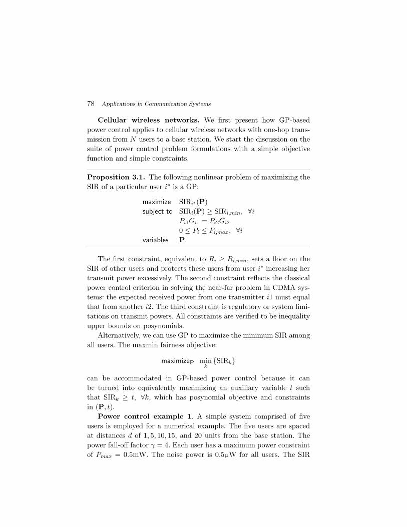
78 Applications in Communication Systems
Cellular wireless networks. We first present how GP-basedpower control applies to cellular wireless networks with one-hop trans-mission from N users to a base station. We start the discussion on thesuite of power control problem formulations with a simple objectivefunction and simple constraints.
Proposition 3.1. The following nonlinear problem of maximizing theSIR of a particular user i∗ is a GP:
maximize SIRi∗(P)subject to SIRi(P) ≥ SIRi,min, ∀i
Pi1Gi1 = Pi2Gi2
0 ≤ Pi ≤ Pi,max, ∀i
variables P.
The first constraint, equivalent to Ri ≥ Ri,min, sets a floor on theSIR of other users and protects these users from user i∗ increasing hertransmit power excessively. The second constraint reflects the classicalpower control criterion in solving the near-far problem in CDMA sys-tems: the expected received power from one transmitter i1 must equalthat from another i2. The third constraint is regulatory or system limi-tations on transmit powers. All constraints are verified to be inequalityupper bounds on posynomials.
Alternatively, we can use GP to maximize the minimum SIR amongall users. The maxmin fairness objective:
maximizeP mink
{SIRk}
can be accommodated in GP-based power control because it canbe turned into equivalently maximizing an auxiliary variable t suchthat SIRk ≥ t, ∀k, which has posynomial objective and constraintsin (P, t).
Power control example 1. A simple system comprised of fiveusers is employed for a numerical example. The five users are spacedat distances d of 1, 5, 10, 15, and 20 units from the base station. Thepower fall-off factor γ = 4. Each user has a maximum power constraintof Pmax = 0.5mW. The noise power is 0.5µW for all users. The SIR
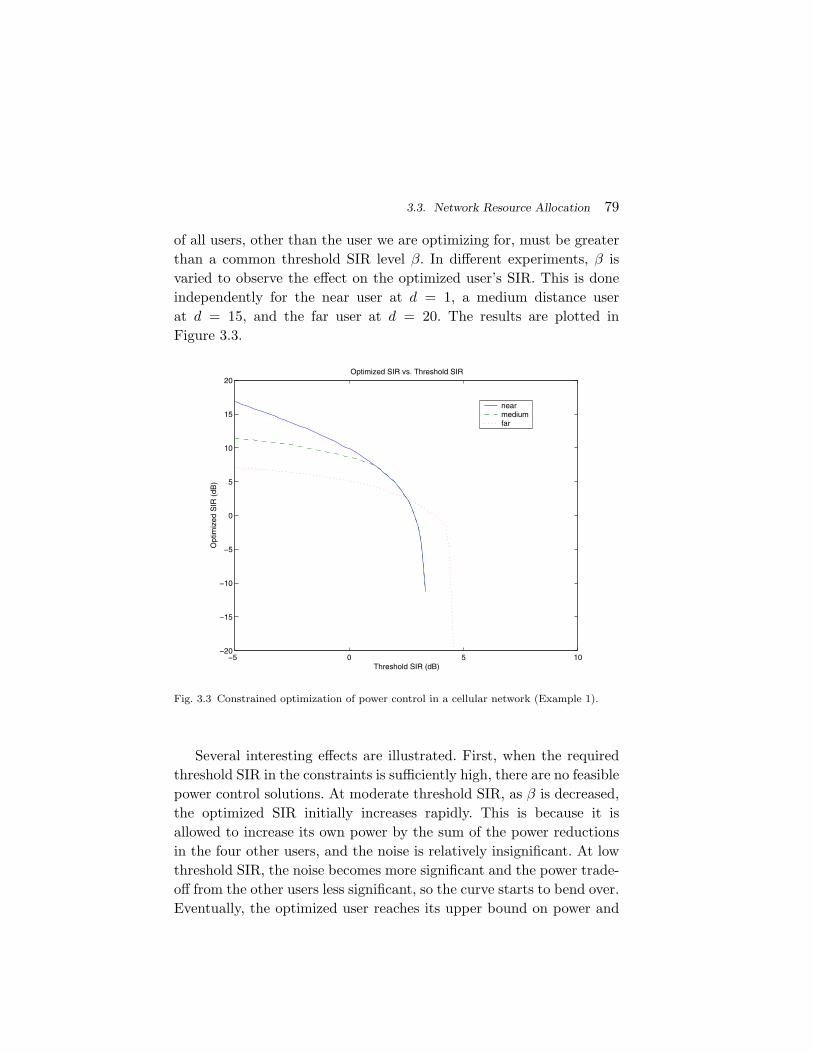
3.3. Network Resource Allocation 79
of all users, other than the user we are optimizing for, must be greaterthan a common threshold SIR level β. In different experiments, β isvaried to observe the effect on the optimized user’s SIR. This is doneindependently for the near user at d = 1, a medium distance userat d = 15, and the far user at d = 20. The results are plotted inFigure 3.3.
−5 0 5 10−20
−15
−10
−5
0
5
10
15
20
Threshold SIR (dB)
Opt
imiz
ed S
IR (
dB)
Optimized SIR vs. Threshold SIR
nearmediumfar
Fig. 3.3 Constrained optimization of power control in a cellular network (Example 1).
Several interesting effects are illustrated. First, when the requiredthreshold SIR in the constraints is sufficiently high, there are no feasiblepower control solutions. At moderate threshold SIR, as β is decreased,the optimized SIR initially increases rapidly. This is because it isallowed to increase its own power by the sum of the power reductionsin the four other users, and the noise is relatively insignificant. At lowthreshold SIR, the noise becomes more significant and the power trade-off from the other users less significant, so the curve starts to bend over.Eventually, the optimized user reaches its upper bound on power and

80 Applications in Communication Systems
cannot utilize the excess power allowed by the lower threshold SIR forother users. Therefore, during this stage, the only gain in the optimizedSIR is the lower power transmitted by the other users. This is exhibitedby the transition from a sharp bend in the curve to a much shallowersloped curve. We also note that the most distant user in the constraintset dictates feasibility.
GP can also be applied to the problem formulations with an overallsystem objective of total system throughput, under both user data rateconstraints and outage probability constraints.
Proposition 3.2. The following nonlinear problem of maximizing sys-tem throughput is a GP:
maximize Rsystem(P)subject to Ri(P) ≥ Ri,min, ∀i
Po,i(P) ≤ Po,i,max, ∀i
0 ≤ Pi ≤ Pi,max, ∀i
variables P.
(3.40)
The objective is equivalent to minimizing the posynomial∏
i ISRi,where ISR is 1
SIR. Each ISR is a posynomial in P and the productof posynomials is again a posynomial. The first constraint is from thedata rate demand Ri,min by each user. The second constraint repre-sents the outage probability upper bounds Po,i,max. These inequalityconstraints put upper bounds on posynomials of P, as can be readilyverified through (3.38,3.39).
There are several obvious variations of problem (3.40) that can besolved by GP, e.g., we can lower bound Rsystem as a constraint andmaximize Ri∗ for a particular user i∗, or have a total power
∑i Pi
constraint or objective function.The objective function to be maximized can also be generalized to a
weighted sum of data rates:∑
i wiRi where w � 0 is a given weight vec-tor. This is still a GP because maximizing
∑i wi log SIRi is equivalent
to maximizing log∏
i SIRwii , which is in turn equivalent to minimizing∏
i ISRwii . Now use auxiliary variables ti, and minimize
∏i t
wii over the
original constraints in (3.40) plus the additional constraints ISRi ≤ ti

3.3. Network Resource Allocation 81
for all i. This is readily verified to be a GP, and is equivalent to theoriginal problem.
In addition to efficient computation of the globally optimal powerallocation with nonlinear objectives and constraints, GP can be usedfor admission control based on GP feasibility study, and for determiningwhich QoS constraint is a performance bottleneck, i.e., meet tightly atthe optimal power allocation, based on GP sensitivity analysis.
Extension: Multihop wireless networks. In wireless multihopnetworks, system throughput may be measured either by end-to-endtransport layer utilities or by link layer aggregate throughput. GPapplication to the first approach will be explained in Subsection 3.4.2,and we focus on the second approach in this subsection, by extendingproblem formulations, such as (3.40), to the multihop case as in thefollowing example.
Power control example 2. Consider a simple four node multihopnetwork shown in Figure 3.4. There are two connections A → B → D
and A → C → D. Nodes A and D, as well as B and C, are sepa-rated by a distance of 20m. Power fall-off factor is −4. Each link hasa maximum transmit power of 1mW. All nodes use MQAM modula-tion. The minimum data rate for each connection is 100bps, and thetarget BER is 10−3. Assuming Rayleigh fading, we require outage prob-ability be smaller than 0.1 on all links for an SIR threshold of 10dB.Spreading gain is 200. Using GP formulation (3.40), we find the maxi-mized system throughput R∗ = 216.8kbps, R∗
i = 54.2kbps for each link,P ∗
1 = P ∗3 = 0.709mW and P ∗
2 = P ∗4 = 1mW. The resulting optimized
SIR is 21.7dB on each link.For this simple network, we also consider an illustrative example
of admission control and pricing. Three new users U1, U2, and U3 aregoing to arrive to the network in order. U1 and U2 require 30kbpssent along the upper path A → B → D, while U3 requires 10kbpssent from A → B. All three users require the outage probability to beless than 0.1. When U1 arrives at the system, her price is the base-line price. Next, U2 arrives, and her QoS demands decrease the maxi-mum system throughput from 216.82kbps to 116.63kbps, so her priceis the baseline price plus an amount proportional to the reduction insystem throughput. Finally, U3 arrives, and her QoS demands produce

82 Applications in Communication Systems
20m
20mA
C
B
D
1 2
3 4
Fig. 3.4 A small wireless multihop network (Example 2).
no feasible power allocation solution, so she is not admitted to thesystem.
Extension: Queuing models. We now turn to delay and bufferoverflow properties to be included in constraints or objective functionof power control optimization. The average delay a packet experiencestraversing a network is an important design consideration in some appli-cations. Queuing delay is often the primary source of delay, particularlyfor bursty data traffic. A node i first buffers the received packets in aqueue and then transmits these packets at a rate R set by the SIRon the egress link, which is in turn determined by the transmit pow-ers P. A FIFO queuing discipline is used here for simplicity. Routingis assumed to be fixed, and is feed-forward with all packets visiting anode at most once.
Packet traffic entering the multihop network at the transmitter oflink i is assumed to be Poisson with parameter λi and to have an expo-nentially distributed length with parameter Γ. Using the model of anM/M/1 queue, the probability of transmitter i having a backlog ofNi = k packets to transmit is well known to be Prob{Ni = k} =(1−ρ)ρk where ρ = λi
ΓRi(P) , and the expected delay is 1ΓRi(P)−λi
. Underthe feed-forward routing and Poisson input assumptions, Burke’s the-orem can be applied. Thus the total packet arrival rate at node i isΛi =
∑j∈I(i) λj where I(i) is the set of connections traversing node i.

3.3. Network Resource Allocation 83
The expected delay Di can be written as
Di =1
ΓRi(P) − Λi. (3.41)
A bound Di,max on Di can thus be written as
1ΓT log2(SIRi) − Λi
≤ Di,max,
or equivalently,ISRi(P) ≤ 2− T
Γ (D−1max+Λi),
which is an upper bound on a posynomial ISR of P.The probability PBO of dropping a packet due to buffer overflow at
a node is also important in several applications. It is again a functionof P and can be written as PBO,i = Prob{Ni > B} = ρB+1 where B
is the buffer size and ρ = ΛiΓRi(P) . Setting an upper bound PBO,i,max
on the buffer overflow probability also gives a posynomial lower boundconstraint in P: ISRi(P) ≤ 2−Ψ where Ψ = TΛi
Γ(PBO,i,max)1
B+1.
Proposition 3.3. The following nonlinear problem of optimizing pow-ers to maximize system throughput, subject to constraints on outageprobability, expected delay, and the probability of buffer overflow, is aGP:
maximize Rsystem(P)subject to Di(P) ≤ Di,max, ∀i
PBO,i(P) ≤ PBO,i,max, ∀i
Same constraints as in problem (3.40)variables P.
(3.42)
Power control example 3. Consider a numerical example ofthe optimal tradeoff between maximizing the system throughput andbounding the expected delay for the network shown in Figure 3.5. Thereare six nodes, eight links, and five multihop connections. All sourcesare Poisson with intensity λi = 200 packets per second, and exponen-tially distributed packet lengths with an expectation of of 100 bits.

84 Applications in Communication Systems
The nodes use CDMA transmission scheme with a symbol rate of 10ksymbols per second and the spreading gain is 200. Transmit powers arelimited to 1mW and the target BER is 10−3. The path loss matrix iscalculated based on a power falloff of d−4 with the distance d, and a sep-aration of 10m between any adjacent nodes along the perimeter of thenetwork.
A
B C
D
E F
1
2
3
4
5
6
7 8
Fig. 3.5 Topology and flows in a multihop wireless network (Example 3).
Figure 3.6 shows the maximized system throughput for differ-ent upper bound numerical values in the expected delay constraints,obtained by solving a sequence of GPs, one for each point on the curve.There is no feasible power allocation to achieve a delay smaller than0.036s. As the delay bound is relaxed, the maximized system through-put increases sharply first, then more slowly until the delay constraintsare no longer active. GP efficiently returns the globally optimal tradeoffbetween system throughput and queuing delay.
SP formulations and solutions for the medium to low SIRcase. There are two main limitations in the GP-based power con-trol methods discussed so far: high-SIR assumption and centralizedcomputation. Both can be overcome as discussed in the rest of thissubsection.
The first limitation is the assumption that SIR is much larger than0dB, which can be removed by the condensation method for SP asintroduced in Subsection 2.2.5. When SIR is not much larger than 0dB,

3.3. Network Resource Allocation 85
0.03 0.04 0.05 0.06 0.07 0.08 0.09 0.1220
230
240
250
260
270
280
290Optimized throughput for different delay bounds
Delay bound (s)
Max
imiz
ed s
yste
m th
roug
hput
(kb
ps)
Fig. 3.6 Optimal tradeoff between maximized system throughput and average delay con-straint (Example 3).
the approximation of log(1+SIR) as log SIR does not hold. Unlike SIR,1+SIR is not an inverted posynomial. Instead, 1
1+SIR is a ratio betweentwo posynomials: ∑
j �=i GijPj + ni∑j GijPj + ni
.
Minimizing or upper-bounding a ratio between two posynomials is anon-convex problem that is intrinsically intractable.
Figure 3.7 shows the approach of GP-based power control for generalSIR regime. In the high SIR regime, we solve only one GP. In themedium to low SIR regimes, we solve truly non-convex power controlproblems that cannot be turned into convex formulations through aseries of GPs.
GP-based power control problems in the medium to low SIR regimesbecome SPs, which can be solved by the single or double conden-sation method. We focus on the single condensation method here.

86 Applications in Communication Systems
Original
OriginalProblem
Problem
(High SIR)
(Medium toLow SIR)
SPComplementaryGP (Condensed)
Solve1 GP
Solve1 GP
Fig. 3.7 GP-based power control for general SIR regime.
Consider a representative problem formulation of maximizing total sys-tem throughput in a cellular wireless network subject to user rate andoutage probability constraints from Proposition 3.2, which is explicitlywritten out as:
minimize∏N
i=11
1+SIRi
subject to (2TRi,min − 1) 1SIRi
≤ 1, i = 1, . . . , N
(SIRth)N−1(1 − Po,i,max)∏N
j �=iGijPj
GiiPi≤ 1,
i = 1, . . . , N
Pi(Pi,max)−1 ≤ 1, i = 1, . . . , N
variables P.
(3.43)
All the constraints are posynomials. However, the objective is not aposynomial, but a ratio between two posynomials. This power controlproblem is a SP (equivalently, a Complementary GP), and can be solvedby the condensation method by solving a series of GPs. Specifically, wehave an algorithm consisting of the following steps:
(0): Choose an initial power vector: a feasible P.(1): Evaluate the denominator posynomial of the (3.43) objective
function with the given P.(2): Compute for each term i in this posynomial,
αi =value of ith term in posynomial
value of posynomial.
(3): Condense the denominator posynomial of the (3.43) objectivefunction into a monomial with weights αi (Subsection 2.2.5).

3.3. Network Resource Allocation 87
(4): Solve the resulting GP e.g., using an interior-point method.(5): Go to STEP 1 using P from step (4).(6): Terminate the kth loop if ‖ P(k) − P(k−1) ‖≤ ε where ε is the
error tolerance.As condensing the objective in the above problem gives us an under-
estimate of the objective value, each GP in the condensation iterationloop tries to improve the accuracy of the approximation to a particularminimum in the original feasible region.
Power control example 4. We consider a wireless cellular networkwith 3 users. Let T = 10−6s, Gii = 1.5, and generate Gij , i �= j, asindependent random variables uniformly distributed between 0 and 0.3.Threshold SIR is SIRth = −10dB, and minimal data rate requirementsare 100 kbps, 600 kbps and 1000 kbps for logical links 1, 2, and 3,respectively. Maximal outage probabilities are 0.01 for all links, andmaximal transmit powers are 3mW, 4mW and 5mW for link 1, 2, and3, respectively.
For each instance of SP power control (3.43), we pick a ran-dom initial feasible power vector P uniformly between 0 and Pmax.We compare the maximized total network throughput achieved overfive hundred sets of experiments with different initial vectors. With the(single) condensation method, SP converges to different optima overthe entire set of experiments, achieving (or coming very close to) theglobal optimum at 5290 bps (96% of the time) and a local optimumat 5060 bps (4% of the time). The average number of GP iterationsrequired by the condensation method over the same set of experimentsis 15 if an extremely tight exit condition is picked for SP condensationiteration: ε = 1 × 10⁻¹⁰. This average can be substantially reduced byusing a larger ε, e.g., increasing ε to 1 × 10⁻² requires on average only4 GPs.
We have thus far discussed a power control problem (3.43) wherethe objective function needs to be condensed. The method is alsoapplicable if some constraint functions are signomials and need to becondensed [37].
The optimum of power control produced by the condensationmethod may be a local one. The following new heuristic of solvinga series of SPs (each solved through a series of GPs) can be further

88 Applications in Communication Systems
applied to help find the global optimum. After the original SP (3.43)is solved, a slightly modified SP is formulated and solved:
minimize t
subject to∏N
i=11
1+SIRi≤ t
t ≤ t0α
Same set of constraints as problem (3.43)variables P, t.
(3.44)
where α is a constant slightly larger than 1. At each iteration of amodified SP, the previous computed optimum value is set to constantt0 and the modified problem (3.44) is solved to yield an objective valuethat is better than the objective value of the previous SP by at leastα. The auxiliary variable t is introduced so as to turn the problemformulation into a SP in (P, t). The starting feasible P for each modifiedSP is picked at random from the feasible set, if any, of the modifiedSP. If we already obtained the global optimal solution in (3.43), then(3.44) would be infeasible, and the iteration of SPs stops.
The above heuristic is applied to the rare instances of power controlexample 4 where solving SP returns a locally optimal power allocation,and is found to obtain the globally optimal solution within 1 or 2 roundsof solving additional SPs (3.44).
Distributed algorithms. As an application of the distributedalgorithm for GP, we maximize the total system throughput in the highSIR regime, assuming the same Pmax at each transmitter. If we directlyapplied the distributed approach described in Subsection 2.3.3, theresulting algorithm would require knowledge by each user of the inter-fering channels and interfering transmit powers, which would trans-late into a large amount of message passing. To obtain a practical dis-tributed solution, we can leverage the structures of the power controlproblems at hand, and instead keep a local copy of each of the effectivereceived powers PR
ij = GijPj and write the problem as follows (afterthe log change of variables to {PR
ij , Pj}):
minimize∑
i log(G−1
ii exp(−Pi)(∑
j �=i exp(PRij ) + ni
))subject to PR
ij = Gij + Pj , ∀i, j
Constraints local to each uservariables {PR
ij }, {Pj}.
(3.45)
3.3. Network Resource Allocation 89
The partial Lagrangian is
L =∑
i
log
G−1
ii exp(−Pi)
∑
j �=i
exp(PRij ) + ni
+∑
i
∑j �=i
γij
(PR
ij −(Gij + Pj
)),
from which the dual variable update is found as
γij (t + 1) = γij (t) + α(t)(PR
ij −(Gij + Pj
))= γij (t) + α(t)
(PR
ij − log GijPj
),
(3.46)
with stepsizes α(t).Each user has to minimize the following partial Lagrangian over(
Pi,{PR
ij
}j
)for given {γij}j , subject to its own local constraints:
Li
(Pi,
{PR
ij
}j, {γij}j
)= log
G−1
ii exp(−Pi)
∑
j �=i
exp(PRij ) + ni
+∑j �=i
γijPRij −
∑
j �=i
γji
Pi.
Two practical observations are in order:
• For the minimization of the above local Lagrangian term,each user only needs to know the term
(∑j �=i γji
)involving
the dual variables from the interfering users, which requiressome message passing.
• For the dual variable update (3.46), each user needs to knowthe effective received power from each of the interfering usersPR
ij = GijPj for j �= i, which in practice may be estimatedfrom the received messages. Hence no explicit message pass-ing is required for this.
With this approach we have avoided the need to know all the inter-fering channels Gij and the powers used by the interfering users Pj .However, each user still needs to know the consistency prices from theinterfering users via some message passing. This message passing can

90 Applications in Communication Systems
be reduced in practice by ignoring the messages from links that arephysically far apart, leading to suboptimal distributed heuristics.
To conclude this subsection, we outline several research issues thatremain to be further explored for GP-based power control: reduction ofSP solution complexity by using high-SIR approximation to obtain theinitial power vector and by solving the series of GPs only approximately(except the last GP), combination of SP solution and distributed algo-rithm for distributed power control in low SIR regime, and applicationto optimal spectrum management in DSL broadband access systemswith interference-limited performance across the tones and among com-peting users sharing a cable binder.
3.3.2 General structure
The applications of standard form GP to power control problemscan be generalized to other constrained optimization of resource allo-cation, and the associated problems of feasibility study, sensitivityanalysis, admission control, and admission pricing, as long as theQoS metrics can be simplified and reduced to the form of invertedposynomials.
Consider n users indexed by i sharing a common pool of communi-cation resource X, such as bandwidth or buffer. The amount of resourceallocated to connection i is denoted by xi. Consider the following Gen-eralized Proportional Allocation (GPA) form, where the total resourceX is allocated to connection i in proportion to some pi and normalizedby a sum of parameters
∑j γji + ανi:
xi =pi∑
j γji + ανiX, ∀i (3.47)
where the allocation parameters pi, νi, γji ≥ 0 belong to a fixed rangeof values for each user i (different ranges for different QoS classes), andα ≥ 0 is a given weight. Usually, there is a tradeoff among the users inresource allocation, i.e., γji are increasing functions of pj .
This form of resource allocation appears in many applications, withpower control being an important special case. A possible explanationof the source from which this form arises can be found in Subsection4.2.1. As a simple example of (3.47), recall the Generalized Processor

3.3. Network Resource Allocation 91
Sharing scheme [100] where an egress link with a total rate of R isshared among multiple connections each receiving rate Ri:
Ri =φi∑j φj
R, ∀i
where {φi} are the parameters that can be directly varied in the systemdesign to produce a desirable R.
As another example, [87] shows that rate control on a single linkthrough the congestion control protocol of TCP Reno produces thefollowing rate allocation proportional to the inverse of round trip delayDi:
Ri =1
Di∑j
1Dj
R, ∀i.
These allocation parameters {pi, νi, γji} can be optimized, withincertain ranges, to maximize the resource received by a particular useri∗ in the highest QoS class, subject to constraints that lower boundthe resources received by each of the other users. Alternatively, formaxmin fairness, allocation parameters can be optimized to maximizethe resource received by the user with the minimum received resource.GP can be used to solve them globally and efficiently.
maximize xi∗ (or maximize minixi)subject to xi ≥ xi,min, ∀i
variables (pi, γji, νi) ≥ lower boundsvariables (pi, γji, νi) ≤ upper bounds.
(3.48)
Theorem 3.4. The optimization problem (3.48) for resource alloca-tion in the GPA form (3.47) is a GP.
The proof is very simple as shown in Appendix B.5, where the keyobservation is that the GPA form is an inverted posynomial. The gen-eral method of distributed solution for GP in Subsection 2.3.3 can alsobe applied to such network resource allocation problems.
As shown in the power control examples in the last subsection, thescope of GP method of efficient resource allocation can be extended

92 Applications in Communication Systems
to accommodate several types of nonlinear functions of the GPA form(which are in turn nonlinear functions of the underlying design vari-ables) in the objective and constraints.
Optimization (3.48) may not have any feasible solution. Indeed, ifthe QoS constraints xi ≥ xi,min,∀i, are too strict, there may exist noresource allocation that simultaneously meets all the constraints. Dueto the GP form of the problem, feasibility of resource allocation in theGPA form can also be efficiently determined, and used for admissioncontrol and pricing in a network: a new user is admitted into the systemonly if the resulted new problem (3.48) is still feasible, and the user ischarged in proportion to the resulting reduction in the objective valueof (3.48).
Furthermore, bottlenecks of resource allocation constraints are read-ily detected, so that if additional resources becomes available, we knowwhere to allocate them to alleviate the bottlenecks of resource demands.Associate a Lagrange dual variable σi ≥ 0 for each resource demandconstraint xi ≥ xi,min. By complementary slackness, if an optimal dualvariable σ∗
1 > 0, then we know that the QoS requirement constraint foruser 1 is tight at optimality, i.e., x∗
1 = x1,min.If the objective is instead to maximize the total resources obtained
by a group of users, then the objective cannot be turned into min-imization of a posynomial, but a ratio between two posynomials. Inthat case, the problem becomes a SP and the condensation or doublecondensation method needs to be applied to solve the problem.
As another example in addition to the power control examples, weshow a simple application of the GP method of resource allocationfor Connection Admission Control (CAC). Consider the ingress of aswitch or a network as shown in Figure 3.8. There are K connectionstrying to get admitted into the system. They first pass through a traf-fic shaping mechanism, such as leaky buckets, to conform the con-nections to their respective provisioned rates λi specified in the QoSservice level agreement. Due to limitation in the available resource, theCAC controller has to enforce admission control among the contendingconnections.
Consider the following simple CAC algorithm where the CAC con-troller has an exponential service time with rate µ. If the first service

3.3. Network Resource Allocation 93
Shaper 1
Shaper 2
Shaper 3
Shaper 4
CAC Controller System
Fig. 3.8 Flows contending for admission into the system through traffic shapers and aconnection admission controller.
time of the CAC controller occurs before any packet from the contend-ing connections arrive at the controller, no connection will be admittedto the system. However, if packets from some connections arrive beforethe first service time of the CAC controller, then the connection whosepacket arrives first will be admitted and the other connections will notbe admitted.
Lemma 3.1. The total rate of admission Ra and the rate of admissionfor each connection Ri (normalized by the maximum total rate) are ofthe following GPA forms:
Ra =∑K
k=1 λk∑Kk=1 λk + µ
,
Ri =λi∑K
k=1 λk + µ, ∀i.
Intuitively, the relative magnitudes of µ and∑K
i=1 λi determine theadmission rate. The relative magnitudes among λi determine the allo-cation among the connections. Using GP we show how the parametersµ and λ can be dynamically optimized to provide a flexible control of

94 Applications in Communication Systems
both the total admission rate and a constrained rate allocation amongthe contending connections.
Proposition 3.4. The following nonlinear problem of maximizing theadmission rate for a particular connection i∗, subject to the total admis-sion rate constraint Ra,max, the QoS constraints of guaranteed rateRi,min for each connection i, and the range constraints on variables λ
and µ, is a GP:
maximize Ri∗(λ, µ)subject to Ra(λ, µ) ≤ Ra,max
Ri(λ, µ) ≥ Ri,min, ∀i
λi,max ≥ λi ≥ λi,min, ∀i
µmax ≥ µ ≥ µmin
variables λ, µ.
(3.49)
Although the first constraint in problem (3.49) is an upperbound instead of the lower bounds on inverted posynomialsas in (3.48), it is still equivalent to a posynomial upper bound(1 − Ra,max)
(∑Kj=1 λjµ
−1 + 1)
≤ 1 due to the specific GPA structurein this case.
Proposition 3.5. The following nonlinear problem of maximizing theadmission rate for the worst-case connection is a GP:
maximize mini Ri(λ, µ)subject to Same constraints as in problem (3.49)variables λ, µ.
(3.50)
Note that that the parameters λi,min, λi,min, µmax and µmax deter-mine the ranges over which λi and µ can vary. Larger the λi,max, higherthe rate connection i could be allowed to receive under the constrainedoptimization. The parameters λi,min and λi,max can be found througha lookup table that maps the QoS class of connection i to the range ofλi allowed. The rate Ri,min guaranteed for each connection can be readfrom the traffic descriptor of the connection.

3.3. Network Resource Allocation 95
As a numerical example, we consider a scenario where there arefive connections contending to get admitted into the system. Problemparameter Ra,max is determined based on the congestion condition ofthe network, and is periodically updated. The connection character-istics and minimum admission requirements are shown in Table 3.2.The connection admission controller varies µ : 0 ≤ µ ≤ 1 and thetraffic shapers vary λ : λi,min ≤ λi ≤ λi,max to control the total sys-tem admission rate and each individual connection’s admission rate bysolving a GP.
Connection λi,min λi,max Ri,min
1 0.21875 0.37500 0.156252 0.18750 0.31250 0.093753 0.25000 0.40625 0.156254 0.28125 0.43750 0.218755 0.09375 0.18750 0.06250
Table 3.2 Arrival traffic bounds and minimum rate requirements.
Figures 3.9 and 3.10 present simulation results illustrating how(λ, µ) are dynamically optimized. The data points for each timeinstance in the graphs are obtained by solving a corresponding GP.In Figure 3.9, (λ, µ) are chosen such that connection 1 admission rateis the largest possible while ensuring that the minimum admission raterequirements Ri,min are met for all other connections, and that the totaladmission rate does not exceed the maximum rate Ra,max allowed bythe system. Connection 1 is always favored over the other connectionswhenever possible under the QoS constraints. For instance, althoughconnection 4 has a higher minimum admission rate requirement thanconnection 1, connection 1 is admitted more often.
In Figure 3.10, (λ, µ) are chosen to maximize the minimum admis-sion rate among all connections, using the same set of Ra,max constraintvalues as in Figure 3.9. With this objective, if there were no minimumadmission rate requirements, all connections would have been admit-ted equally. However, because different connections have different char-acteristics and requirements, admission rates will vary. Connections

96 Applications in Communication Systems
0 5 10 15 20 25 30 35 40 45 500
0.1
0.2
0.3
0.4
0.5
0.6
0.7
0.8
0.9
1Flow Admission Rate Over Time
Adm
isio
n R
ate
Time
Flow 1 admission rateFlow 2 admission rateFlow 3 admission rateFlow 4 admission rateFlow 5 admission rateTotal admission rate allowed
Fig. 3.9 Optimized CAC: Maximize the admission rate for connection 1.
that have relatively small minimum admission rate requirements (e.g.,connections 2 and 5) are usually admitted at rates higher thanrequested. Intuitively, in Figure 3.10 all connections are treated asequally as possible, resulting in a narrower band of admission ratecurves.
3.4 Network Congestion Control
Materials in this subsection are in part based on [31, 88].
3.4.1 TCP Vegas congestion control
Transmission Control Protocol (TCP) is one of the two widely-usedtransport layer protocols in the Internet. A main function performedby TCP is network congestion control and end-to-end rate allocation.Roughly speaking, there are two phases of TCP congestion control:

3.4. Network Congestion Control 97
0 5 10 15 20 25 30 35 40 45 500
0.1
0.2
0.3
0.4
0.5
0.6
0.7
0.8
0.9
1Flow Admission Rate Over Time
Adm
isio
n R
ate
Time
Flow 1 admission rateFlow 2 admission rateFlow 3 admission rateFlow 4 admission rateFlow 5 admission rateTotal admission rate allowed
Fig. 3.10 Optimized CAC: Maximize the minimum admission rate among all connections.
slow start and congestion avoidance. Long-lived flows usually spendmost of the time in congestion avoidance. Similar to recent work onutility maximization models of TCP, we assume a deterministic flowmodel for the average, equilibrium behavior of the congestion avoid-ance phase. TCP uses sliding windows to adjust the allowed trans-mission rate at each source based on implicit or explicit feedbackof the congestion signals generated by Active Queue Management(AQM) at the routers. Among the variants of TCP, such as Tahoe,Reno, Vegas, and FAST, some use loss as the congestion signal andothers use delay. Delay-based congestion signals, like those in TCPVegas, have more desirable properties on convergence, stability, andfairness [87].
The basic rate allocation mechanism of TCP Vegas is as follows.Let ds be the propagation delay along the path originating from sources, and Ds be the propagation plus congestion-induced queuing delay.Obviously ds = Ds when there is no congestion on all the links used

98 Applications in Communication Systems
by source s. The window size ws is updated at each source s accordingto whether the difference between the expected rate ws
dsand the actual
rate wsDs
, where Ds is estimated by the timing of ACK packets, is smallerthan a parameter αs:
ws(t + 1) =
ws(t) + 1Ds(t) if ws(t)
ds− ws(t)
Ds(t) < αs
ws(t) − 1Ds(t) if ws(t)
ds− ws(t)
Ds(t) > αs
ws(t) else.
The end-to-end throughput for each path is the allowed source rate xs,which is proportional to the window size: xs(t) = ws(t)
Ds(t) .Since the seminal work by Kelly et al. [77] that analyzes network
rate allocation as a distributed solution of utility maximization, TCPcongestion control mechanisms have been shown as approximated dis-tributed algorithms solving appropriately formulated utility maximiza-tion problems (e.g., [79, 81, 85, 86, 87, 88, 89, 95, 96, 117]). A centralapproach in this series of work is to interpret source rates as primalvariables, link congestion measures as dual variables, and a TCP–AQMprotocol as a distributed algorithm over the Internet implicitly to solvethe following network utility maximization.
Consider a wired communication network with L links, each with afixed capacity of cl bps,6 and S sources, each transmitting at a sourcerate of xs bps. Each source emits one flow, using a fixed set L(s) ofconnected links in its path, and has an increasing, strictly concave, andtwice differentiable utility function Us(xs). Network utility maximiza-tion is the problem of maximizing the total utility
∑s Us(xs) over the
source rates x, subject to linear flow constraints∑
s:l∈L(s) xs ≤ cl forall links l:
maximize∑
s Us(xs)subject to
∑s:l∈L(s) xs ≤ cl, ∀l
x � 0variables x.
(3.51)
Different TCP-AQM protocols solve for different strictly concaveutility functions using different types of congestion signals. For exam-ple, TCP Vegas is shown [88] to be implicitly solving (3.51) for weighted
6 Capacity in terms of attainable throughput with a given code and modulation, not theinformation theoretic limit of channel capacity.

3.4. Network Congestion Control 99
logarithmic utility functions: Us(xs) = αsds log xs, using queuing delaysas congestion signals. Although TCP and AQM protocols were designedand implemented without regard to utility maximization, now they canbe reverse-engineered to determine the underlying utility functions andto rigorously characterize many important equilibrium and dynamicproperties.
In particular, TCP Vegas has been reverse-engineered as a dis-tributed algorithm implicitly solving the following logarithmic networkutility maximization problem:
maximize∑
s αsds log xs
subject to∑
s:l∈L(s) xs ≤ cl, ∀l
x � 0variables x.
(3.52)
This Vegas problem is readily seen to be a GP as in Extension 6 in Sub-section 2.2.1. As discussed in Subsection 2.3.3 and the next subsection,this GP can be distributively solved by a Lagrangian decompositionof the coupling (flow conservation) constraint. TCP Vegas congestioncontrol solves this GP using queuing delay as the dual variables, i.e.,the link congestion prices.
It is also known [77] that the weighted log utility functions implic-itly maximized by TCP Vegas lead to a weighted proportionally fairallocation of link capacities, i.e., given the optimizer x∗ to (3.52),the following inequality holds for any x that satisfies the constraintof (3.52): ∑
s
αsdsxs − x∗
s
x∗s
≤ 0.
3.4.2 Jointly optimal congestion and power control
Consider a wireless network with multihop transmission andinterference-limited link rates. Congestion control mechanisms, suchas those in TCP, regulate the allowed source rates so that the totaltraffic load on any link does not exceed the available capacity. At thesame time, the attainable data rates on wireless links depend on theinterference levels, which in turn depend on the power control policy.

100 Applications in Communication Systems
This subsection describes a distributed algorithm for jointly optimalend-to-end congestion control and per-link power control. The algo-rithm utilizes the coupling between the transport and physical layersto increase end-to-end throughput and to enhance energy efficiency ina wireless multihop network.
This presents a step towards understanding ‘layering’ as ‘opti-mization decomposition’, where the overall communication networkis modeled by a generalized utility maximization problem, each layercorresponds to a decomposed subproblem, and the interfaces amonglayers are quantified as functions of primal or dual variables coor-dinating the subproblems. In the case of the transport and physi-cal layers, link congestion prices turn out to be the optimal ‘layeringprices’.
Network utility maximization problems are linearly constrained bylink capacities that are assumed to be fixed quantities. However, net-work resources can sometimes be allocated to change link capacities.This formulation of network utility maximization with ‘elastic’ linkcapacities [31, 99, 131] leads to a new approach of congestion avoid-ance in wireless multihop networks. The current approach of congestioncontrol in the Internet is to avoid the development of a bottleneck linkby reducing the allowed transmission rates from all the sources usingthis link. Intuitively, an alternative approach is to build, in real time,a larger transmission ‘pipe’ and ‘drain’ the queued packets faster on abottleneck link. Indeed, a smart power control algorithm would allo-cate just the ‘right’ amount of power to the ‘right’ nodes to alleviatethe bottlenecks, which may then induce an increase in end-to-end TCPthroughput. But there are two major difficulties in making this ideawork: defining which link constitutes a ‘bottleneck’ a priori is diffi-cult, and changing the transmit power on one link also affects the datarates available on other links. Due to interference in wireless networks,increasing the capacity on one link reduces those on other links. Weneed to find an algorithm that distributively and adaptively detectsthe ‘bottleneck’ links and optimally ‘shuffles’ them around in thenetwork.
Consider a wireless multihop network with N nodes and an estab-lished logical topology and routing, where some nodes are sources of

3.4. Network Congestion Control 101
transmission and some nodes act as ‘voluntary’ relay nodes. A seq-uence of connected links l ∈ L(s) forms a route originating fromsource s. Let xs be the transmission rate of source s, and cl be thecapacity on logical link l. Revisiting the utility maximization formula-tion (3.51), for which TCP congestion control solves, we observe thatin an interference-limited wireless network, data rates attainable onwireless links are not fixed numbers c as in (3.51), and instead canbe written, in the high SIR regime, as a global and nonlinear func-tion of the transmit power vector P and channel conditions: cl(P) =1T log(KSIRl(P)).
With the above model, we have specified the following networkutility maximization with ‘elastic’ link capacities and logarithmicutilities:
maximize∑
s αsds log xs
subject to∑
s:l∈L(s) xs ≤ cl(P), ∀l
x,P � 0variables x,P.
(3.53)
The key difference from the standard utility maximization (3.51) is thateach link capacity cl is now a function of the new optimization variables:the transmit powers P. The design space is enlarged from x to both xand P, which are clearly coupled in (3.53). Linear flow constraints onx become nonlinear constraints on (x,P). In practice, problem (3.53)is also constrained by the maximum and minimum transmit powersallowed at each transmitter on link l: Pl,min ≤ Pl ≤ Pl,max, ∀l.
In the context of wireless ad hoc networks, new distributed algo-rithms are needed to solve (3.53). Thus the major challenges are thetwo global dependencies:
• Source rates x and link capacities c are globally coupledacross the network, as reflected in the range of summation{s : l ∈ L(S)} in the constraints in (3.53).
• Each link capacity cl(P) is a global function of all the inter-fering powers.
The following distributive algorithm converges to the joint andglobal optimum of (3.53).

102 Applications in Communication Systems
Jointly Optimal Congestion-control and Power-control(JOCP) Algorithm [31]:During each time slot t, the following four updates are carried outsimultaneously until convergence:
(1) At each intermediate node, a weighted queuing delay λl isimplicitly updated,7 where γ > 0 is a constant weight:
λl(t + 1) =
λl(t) +
γ
cl(t)
∑
s:l∈L(s)
xs(t) − cl(t)
+
. (3.54)
(2) At each source, total delay Ds is measured and used toupdate the TCP window size ws. Consequently, the sourcerate xs is updated:
ws(t + 1) =
ws(t) + 1Ds(t) if ws(t)
ds− ws(t)
Ds(t) < αs
ws(t) − 1Ds(t) if ws(t)
ds− ws(t)
Ds(t) > αs
ws(t) else.
(3.55)
xs(t + 1) =ws(t + 1)
Ds(t).
(3) Each transmitter j calculates a message mj(t) ∈ R+ basedon locally measurable quantities, and passes the message toall other transmitters by a flooding protocol:
mj(t) =λj(t)SIRj(t)
Pj(t)Gjj.
(4) Each transmitter updates its power based on locally measur-able quantities and the received messages, where κ > 0 is aconstant weight:
Pl(t + 1) = Pl(t) +κλl(t)Pl(t)
− κ∑j �=l
Gljmj(t). (3.56)
7 This is using an average model for deterministic fluids. The difference between the totalingress flow intensity and the egress link capacity, divided by the egress link capacity, givesthe average time that a packet needs to wait before being sent out on the egress link.

3.4. Network Congestion Control 103
With the maximum and minimum transmit power constraint(Pl,max, Pl,min) on each transmitter, the updated power isprojected onto the interval [Pl,max, Pl,min].
We first present some intuitive arguments on this algorithm beforeproving the convergence theorem and discussing the practical imple-mentation issues. Item (2) is simply the TCP Vegas window update[23]. Item (1) is a modified version of queuing delay price update [88](and the original update [23] is an approximation of item (1)). Items(3) and (4) describe a new power control using message passing [32].
Taking in the current values of λj(t)SIRj(t)Pj(t)Gjj
as the messages from othertransmitters indexed by j, the transmitter on link l adjusts its powerlevel in the next time slot in two ways: first increase power directlyproportional to the current price (e.g., queuing delay in TCP Vegas)and inversely proportional to the current power level, then decreasepower by a weighted sum of the messages from all the other transmit-ters, where the weights are the path losses Glj . Intuitively, if the localqueuing delay is high, transmit power should increase, with more mod-erate increase when the current power level is already high. If queuingdelays on other links are high, transmit power should decrease in orderto reduce interference on those links.
Note that to compute mj , the values of queuing delay λj , signal-interference-ratio SIRj , and received power level PjGjj can be directlymeasured by node j locally. This algorithm only uses the resultingmessage mj but not the individual values of λj , SIRj , Pj and Gjj . Eachmessage is simply a real number.
The known source algorithm (3.55) and queue algorithm (3.54) ofTCP-AQM, together with the new power control algorithm (3.56),form a set of distributed, joint congestion control and resource allo-cation in wireless multihop networks. As the transmit powers change,SIR and thus data rate also change on each link, which in turnchange the congestion control dynamics. At the same time, conges-tion control dynamics change the dual variables λ(t), which in turnchange the transmit powers. Figure 3.11 shows this nonlinear cou-pling of ‘supply’ (regulated by power control) and ‘demand’ (regu-lated by congestion control), through the same shadow prices λ that

104 Applications in Communication Systems
are currently used by TCP to regulate distributed demand. Now λ
serves the second function of cross-layer coordination in the JOCPAlgorithm.
Shadow Price
(Supply)(Demand)
Shadow Price Shadow Price
P
cx
x
Power ControlTransmit Node
TCP Source Node
Node QueueIntermediate
Fig. 3.11 Nonlinearly coupled dynamics of joint congestion and power control.
Notice that there is no need to change the existing TCP conges-tion control and queue management algorithms. All that is needed toachieve the joint and global optimum of (3.53) is to utilize the valuesof weighted queuing delay in designing power control algorithm in thephysical layer.8
The advantage of such a joint control can be captured in a smallillustrative example, where the logical topology and routes for fourmulti-hop connections are shown in Figure 3.12. Sources at each of thefour flows use TCP Vegas window updates with αs ranging from 3 to 5.The path losses Gij are determined by the relative physical distancesdij , which we vary in different experiments, by Gij = d−4
ij . The targetBER is 10−3 on each logical link.
4
32
1
Fig. 3.12 The logical topology and routes in an illustrative example.
Transmit powers, as regulated by the proposed distributed powercontrol, and source rates, as regulated through TCP Vegas window
8 This approach is complementary to some recent suggestions in the Internet communityto pass physical layer information for a better control of routing and congestion in upperlayers.

3.4. Network Congestion Control 105
update, are shown in Figure 3.13. The initial conditions of the graphsare based on the equilibrium states of TCP Vegas with fixed powerlevels of 2.5mW. With power control, the transmit powers P distribu-tively adapt to induce a ‘smart’ capacity c and queuing delay λ con-figuration in the network, which in turn lead to increases in end-to-endthroughput as indicated by the rise in all the allowed source rates.Notice that some link capacities actually decrease while the capaci-ties on the bottleneck links rise to maximize the total network utility.This is achieved through a distributive adaptation of power, whichlowers the power levels that cause most interference on the links thatare becoming a bottleneck in the dynamic demand-supply balancingprocess. Confirming our intuition, such a ‘smart’ allocation of powertends to reduce the spread of queuing delays, thus preventing anylink from becoming a bottleneck. Queuing delays on the four links donot become the same though, due to the asymmetry in traffic loadon the links and different weights in the logarithmic utility objec-tive functions. The end-to-end throughput per watt of power trans-mitted, i.e., the throughput-power ratio, is 82% higher with powercontrol.
We can associate a Lagrange multiplier λl for each of the constraints∑s:l∈L(s) xs ≤ cl(P). To find the stationary points of the Lagrangian,
we need to solve the following Lagrangian maximization problems:Isystem(x,P,λ) = (
∑s αsds log xs − ∑
l λl∑
s:l∈L(s) xs) + (∑
l λlcl(P)).By linearity of the differentiation operator, this can be decomposedinto two separate maximization problems:
maximizex0∑s
αsds log xs −∑s
∑l∈L(s)
λlxs
maximizeP0∑
l
λlcl(P).
Both maximization problems are readily verified to be GPs, one inx and another in P. The first maximization is already implicitly solvedby the TCP Vegas congestion control mechanism. But we still need tosolve the second maximization, using the Lagrange multipliers λ as theshadow prices to allocate exactly the right power to each transmitter.Since the data rate on each wireless link is a global function of all the
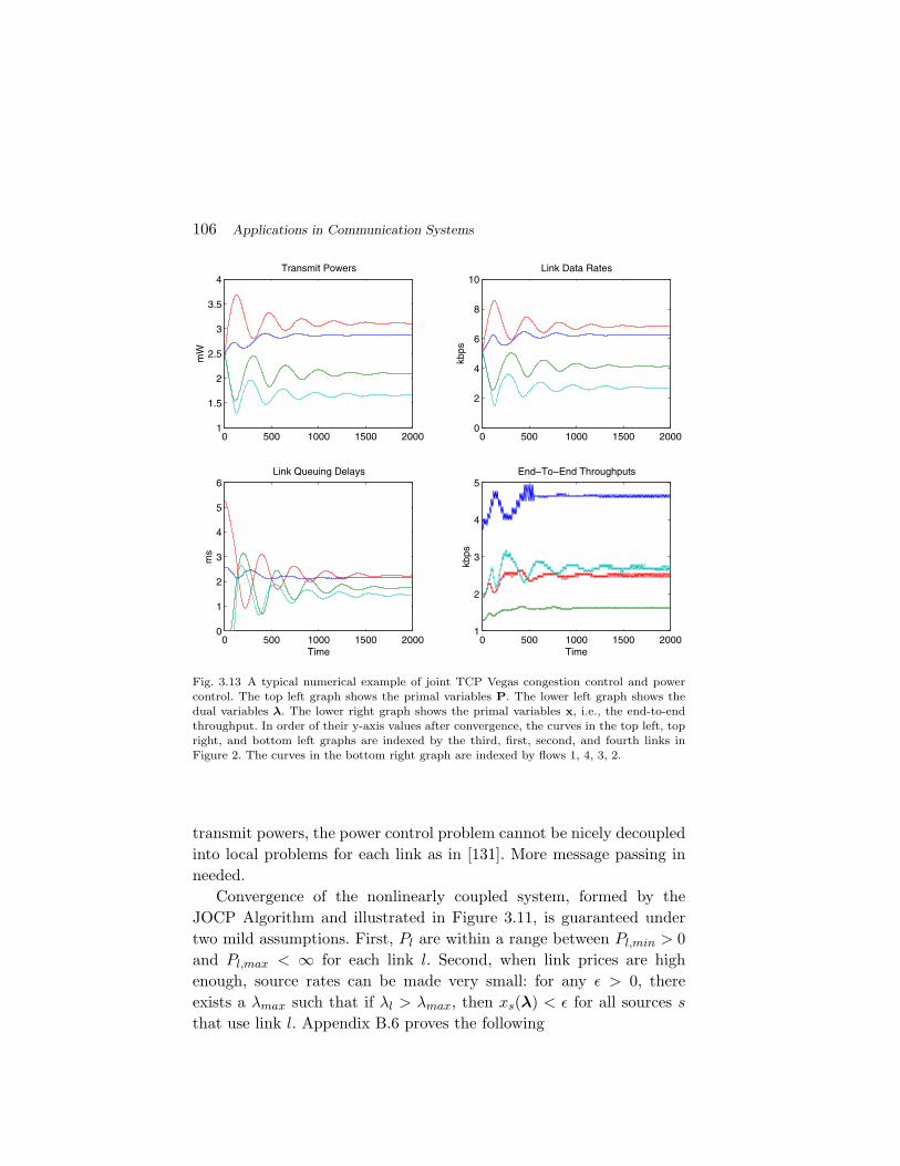
106 Applications in Communication Systems
0 500 1000 1500 20001
1.5
2
2.5
3
3.5
4Transmit Powers
mW
0 500 1000 1500 20000
2
4
6
8
10Link Data Rates
kbps
0 500 1000 1500 20000
1
2
3
4
5
6Link Queuing Delays
Time
ms
0 500 1000 1500 20001
2
3
4
5End−To−End Throughputs
Time
kbps
Fig. 3.13 A typical numerical example of joint TCP Vegas congestion control and powercontrol. The top left graph shows the primal variables P. The lower left graph shows thedual variables λ. The lower right graph shows the primal variables x, i.e., the end-to-endthroughput. In order of their y-axis values after convergence, the curves in the top left, topright, and bottom left graphs are indexed by the third, first, second, and fourth links inFigure 2. The curves in the bottom right graph are indexed by flows 1, 4, 3, 2.
transmit powers, the power control problem cannot be nicely decoupledinto local problems for each link as in [131]. More message passing inneeded.
Convergence of the nonlinearly coupled system, formed by theJOCP Algorithm and illustrated in Figure 3.11, is guaranteed undertwo mild assumptions. First, Pl are within a range between Pl,min > 0and Pl,max < ∞ for each link l. Second, when link prices are highenough, source rates can be made very small: for any ε > 0, thereexists a λmax such that if λl > λmax, then xs(λ) < ε for all sources s
that use link l. Appendix B.6 proves the following

3.5. Queuing Theory 107
Theorem 3.5. For small enough constants γ and κ, the distributedJOCP Algorithm (3.54,3.55,3.56) converges to the global optimum ofthe joint congestion control and power control problem (3.53).
Extensions to other TCP variants and multi-commodity flow rout-ing are discussed in [31]. Other properties of this distributed algorithmof GP are shown: the convergence is geometric, can be maintained underfinite asynchronism, is robust to estimation error of path loss and topacket loss due to channel fading, and can be accelerated by passingslightly more information among the nodes. Simplified heuristics forpartial messaging are also possible.
3.5 Queuing Theory
Materials in this subsection are in part based on [36, 68, 76].Queuing systems form a fundamental part for different types of
communication systems, such as computer multiprocessor networksand communications data networks. Queuing systems are also an inte-gral part of various network elements, such as the input and outputbuffers of a packet switch. We often would like to optimize some per-formance metrics of queuing systems, for example, buffer occupancy,overall delay, jittering, workload, and probabilities of certain states.However, optimizing the performance of even simple queues like theM/M/m/m queue is in general a difficult problem because of the non-linearity of the performance metrics as functions of the arrival andservice rates.
We show how convexity properties of queuing systems, in the form ofposynomials (that appear as product form distributions) and log-sum-exp functions (that appear in effective bandwidth formulations), canbe used to turn some of these problems into polynomial time solvableones. We provide a suite of GP formulations to efficiently and globallyoptimize the performance of queuing systems under QoS constraints,first for single Markovian queues, then for blocking probability mini-mization and service rate allocation through the effective bandwidthapproach, and finally for closed networks of queues.
First consider a simple example of minimizing the service load ofan M/M/1 queue, over the arrival rate λ and service rate µ, with

108 Applications in Communication Systems
constraints on average queuing delay W , total delay D, and queueoccupancy Q. The following proposition can be readily verified throughbasic formulas of M/M/1 queues [15]:
Proposition 3.6. The following nonlinear optimization of service loadminimization is a GP:
minimize µλ
subject to W ≤ Wmax
D ≤ Dmax
Q ≤ Qmax
λ ≥ λmin
µ ≤ µmax
variables λ, µ.
(3.57)
The constant parameters are the performance upper bounds Wmax,Dmax and Qmax, and practical constraints on the maximum servicerate µmax of the queue that cannot be exceeded, and the minimumincoming traffic rate λmin that must be supported.
The above formulation can be extended to a Markovian queuingsystem with N queues sharing a pool of service rate bounded by µmax
(for example, connected to a common egress link). The arrival rate tobe supported for each individual queue i is bounded by λi,min. Thereare delay and queue occupancy bounds Wi,max, Di,max and Qi,max foreach queue i. The objective now becomes minimizing a weighted sumof the service loads for all the queues, with constant weights α:
Corollary 3.4. The following nonlinear minimization of a weightedsum of service loads is a GP:
minimize∑N
i=1 αiµiλi
subject to Wi ≤ Wi,max, ∀i
Di ≤ Di,max, ∀i
Qi ≤ Qi,max, ∀i
λi ≥ λi,min, ∀i∑Ni=1 µi ≤ µmax
variables λ,µ.
(3.58)

3.5. Queuing Theory 109
We now optimize specific queue occupancy probabilities of anM/M/m/m queue. The steady state probability of state k is given by
pk =(λ
µ)k 1k!∑m
i=0(λµ)i 1
i!
.
In many applications of queuing systems to network design, we wouldlike to maximize the probability of a particular desirable state, withoutmaking the probabilities of other states too small. For example, we maywant to design a telephone call service center so as to maximize theprobability that a particular number of telephone lines (e.g., 90%) arein use at any given time.
Proposition 3.7. The following nonlinear optimization ofM/M/m/m queues is a GP:
maximize pk(λ, µ)subject to pj(λ, µ) ≥ Cj , ∀j
λ ≥ λmin
µ ≤ µmax
variables λ, µ.
(3.59)
The constant parameters are λmin, µmax and Cj , j = 1, 2, . . . , m.
One approach to study the buffer overflow probability is throughthe blocking probability of an M/M/1/B queue with a fixed buffer ofsize B:
pB =(λ
µ)B 1B!∑B
i=0(λµ)i 1
i!
.
Minimizing pB is equivalent to maximizing a posynomial of λ and µ,which is in turn equivalent to maximizing a convex function. There-fore, minimizing blocking probability cannot be turned into a GP. Onepossible heuristic is to use GP to maximize the probability of somestate k, k < B, subject to lower bounds on pj for all other j < B. SincepB = 1 − ∑B−1
i=0 pi, this heuristic essentially minimizes the blockingprobability.

110 Applications in Communication Systems
An alternative way to characterize buffer overflow is through thelarge deviation approach, where the blocking probability is guaranteedstatistically: for a connection X with a prescribed service rate R in thequeue, we would like to ensure that the probability of overflow (receiv-ing more than R bps from X) over a time scale of t is exponentiallysmall:
Prob
{t∑
i=1
X(i) ≥ R
}≤ exp(−sR) (3.60)
where s ≥ 0 is the under-subscription factor. Smaller s implies moreaggressive statistical multiplexing of multiple connections to one queue.This number R is called the effective bandwidth EB of X (as firstproposed in [68], used in many papers since, and nicely reviewed in [76]).
Using the Chernoff bound, the effective bandwidth is given by
EB(X) =1st
log E [exp(sX)] . (3.61)
In practice, the expectation is replaced by the empirical average oftraffic data over a time period of t that is much larger than the timescale factor t:
EB(X) =1st
log
t
t
tt∑
i=1
exp(sX(i))
where X(i) is the number of bits sent by connection X during the ithtime slot.
In traffic engineering, we want to either minimize the assigned ser-vice rate EB(X) subject to constraints that lower bound the trafficintensity {X(i)} to be supported (i.e., exponentially small probabilityof overflow or blocking), or maximize the traffic intensity subject toconstraints upper bounding the service rate that can be assigned to X.Both problems can be formulated as GPs, and we focus on the first for-mulation here. Constraints on the minimal level of traffic intensity to besupported by EB(X) are indexed by j and induced by the stochasticityof other connections sharing the queue buffer.

3.5. Queuing Theory 111
Proposition 3.8. The following nonlinear problem of constrainedbuffer allocation is a GP:
minimize EB(X)subject to
∑i PijX(i) ≥ Xmin,j , ∀j
variables X(i), ∀i.
(3.62)
The constant parameters are Pij and Xmin,j .
A numerical example is summarized as follows. With s = 0.5, t =5ms, we impose a set of 10 different constraints to specify the type of anarrival curve a queue should be able to support without blocking. TheGP solution returns the minimized effective bandwidth as EB∗(X) =1.7627Mbps, and the envelope of supportable arrival curves is shownin Figure 3.14. Connections with arrival curves below this envelopewill not cause buffer overflow or queue blocking with a probabilisticguarantee as in (3.60).
0 10 20 30 40 50 60 70 800
0.5
1
1.5
2
2.5
3Arrival curve constraint envolope
Time (ms)
Num
ber
of b
its a
llow
ed in
eac
h m
s (k
b)
Fig. 3.14 The envelope of arrival curves supportable by EB∗(X) = 1.7627.
In some queuing problems, a fixed number of customers or taskscirculate indefinitely in a closed network of queues. For example, some

112 Applications in Communication Systems
computer system models assume that at any given time a fixed numberof programs occupy the resource. Such problems can be modeled by aclosed queuing network consisting of K nodes, where each node k con-sists of mk identical exponential servers, each with an average servicerate µk. There are always exactly N customers in the system. Onceserved at node k, a customer goes to node j with probability pkj . Thenfor each node k, the average arrival rate to the node, λk, is given byλk =
∑Kj=1 pkjλj .
The steady state probability that there are nk customers in node k,for k = 1, 2, . . . , K, is given by a closed network Jackson’s theorem:
Prob(n1, n2, . . . , nK) =1
G(K)
K∏k=1
(λkµk
)nk
βk(nk),
where
βk(nk) =
{nk! nk ≤ mk
mk!mnk−mkk nk > mk,
and the normalization constant G(K) is given by
G(K) =∑s
K∏k=1
(λkµk
)nk
βk(nk)
where the summation over s is taken over all state vectors s =(n1, n2, . . . , nK) satisfying
∑Kk=1 nk = N .
Proposition 3.9. The following nonlinear problem of maximizing theprobability of state (n1 = n∗
1, . . . , nK = n∗K) with
∑Kk=1 nk = N , sub-
ject to constraints on other states, is a GP:
maximize Prob(n1 = n∗1, . . . , nK = n∗
K)subject to Prob(n1, . . . , nK) ≥ Constant
µk,min ≤ µk ≤ µk,max, ∀k∑Kk=1 mkµk ≤ µtotal
variables µ
(3.63)
where there is a constraint of the first type for each steadystate probability Prob(n1, . . . , nK). The constant parameters areµk,min, µk,max, mk, k = 1, 2, . . . , K, and µtotal.

3.5. Queuing Theory 113
The above optimization problem can be viewed as a problem ofresource (i.e., service capacity µ) allocation in a closed queuing net-work. The goal is to maximize the probability that the system is in aparticular state subject to constraints on other states and the limitedsystem resource µtotal.


4Why Is Geometric Programming Useful for
Communication Systems
The last section summarizes GP’s applications to information theoryand queuing theory, coding and signal processing, network resourceallocation and protocols. This section initiates an exploration of theplausible reasons why GP is useful to such a variety of topics in the anal-ysis and design of communication systems.
4.1 Stochastic Models
Materials in this subsection are in part based on [30, 42, 45, 52, 108].Many problems in information theory, queuing theory, and coding
are based on stochastic models of communication systems, where theprobability of an undesirable event is to be bounded or minimized. Forexample, given a family of conditional distributions describing a channel,we would like the probability of decoding error to vanish exponentially asthe codeword length goes to infinity. Or given a queuing discipline andarrival and departure statistics, we would like the probability of bufferoverflow to vanish exponentially as the buffer size increases.
Large deviation principles govern such exponential behavior instochastic systems. It is well known that convex analysis is closely
115

116 Why Is Geometric Programming Useful for Communication Systems
related to large deviation principles [45, 127]. In Subsection 4.1.2 wewill sharpen this general connection by showing that several importantlarge deviation bounds can be computed by GP. It is this connectionbetween GP and large deviation characterizations that is the underly-ing reason for GP’s applicability to communication system problemsbased on stochastic models.
This discussion is first motivated in Subsection 4.1.1 by examin-ing the relationship between GP and classical statistical physics. Suchrelationships were recognized since the 1960s [52] and is not surprisingas one can easily realize that the log-sum-exp function, which can bethe objective or constraint functions of a convex form GP, is the logpartition function of the Boltzmann distribution. A posynomial canbe transformed into not just a convex function, but also one in the‘right’ convexity structure with interesting interpretations from statis-tical physics.
4.1.1 Interpretations from statistical physics
Consider a system governed by classical statistical physics with n
states at temperature T , where each state i has energy ei and prob-ability pi of occurring. Given an energy vector e and a probabilityvector p, the average energy is U(p, e) = pTe and the entropy isH(p) = −∑n
i=1 pi log pi. The Gibbs free energy is defined as a weighteddifference between the two:
G(p, e) = U(p, e) − TH(p) = pTe + Tn∑
i=1
pi log pi.
Solving the problem of Gibbs free energy minimization:
minimize pTe + T∑n
i=1 pi log pi
subject to 1Tp = 1p � 0
variables p
(4.1)
with constant parameters e, is important in statistical physics with sev-eral interpretations, e.g., (4.1) strikes a balance between energy mini-mization and entropy maximization.

4.1. Stochastic Models 117
Following the argument in the discussion of the conjugacy relation-ship between log-sum-exp and negative entropy in Subsection 2.1.1, it iseasy to see that the Boltzmann distribution, denoted by b, minimizesG(p, e) over p for a given energy vector e, where bi is proportionalto exp(− ei
T ). The proportionality constant needed for normalization iscalled the partition function Z(e) =
∑ni=1 exp(−ei
T ). The Gibbs freeenergy G(p, e) induced by the Boltzmann distribution p = b is calledthe Helmholtz free energy F (e), which is the negative logarithm of Z(e)scaled by T :1
F (e) = G(b, e) = −T logn∑
i=1
exp(−ei
T).
Due to the convexity of the Gibbs free energy in p and the con-cavity of the Helmholtz free energy in e, maxe minp G(p, e) =minp maxe G(p, e). Therefore, maximizing the Helmholtz free energyis equivalent to finding the minimum Gibbs free energy for the worst-case energy vector.
The Gibbs free energy can also be generalized as follows [108]. Con-sider a multiple phase chemical system with K phases and J types ofsubstances. Let njk be the number of atomic weights of substance j
that are in phase k, and let ejk be the energy of substance j in phase k,j = 1, 2, . . . , J, k = 1, 2, . . . , K. The multiphase equilibrium problemis to minimize the following generalized Gibbs free energy with unittemperature over {njk}:
∑j,k
njkejk +∑j,k
njk log
(njk∑j′ nj′k
). (4.2)
Now suppose the distribution on the states is not the Boltzmanndistribution b, but some general distribution q. In this case, we willget a corresponding value for the Gibbs free energy G(q, e), and the
1 With a logarithmic transformation of variables: ei = − log pi, ∀i, it is easy to see that theRenyi entropy (3.33) is a log-sum-exp function. If the order of the Renyi entropy is 1/T ,the Renyi entropy is a scaled Helmholtz free energy:
Hγ(p) =1
T − 1F (e).

118 Why Is Geometric Programming Useful for Communication Systems
difference between this value and the Helmholtz free energy, normalizedby the temperature T , is given by:
1T
(G(q, e) − G(b, e)
)=
qTeT
−H(q)− F (e)T
=n∑
i=1
qi logqi
bi
= D(q‖b).
(4.3)Therefore, another way to derive the Boltzmann distribution is
through minimizing the difference between a general Gibbs free energyand the Helmholtz free energy, expressed as a KL divergence (rela-tive entropy), over the probability simplex. Minimizing KL divergenceD(q‖b) over q is precisely the dual objective function of an uncon-strained GP. Indeed, we can rewrite the dual objective in (2.7) as a KLdivergence minimization: minimizeνD(ν‖d), or in the exponentiatedform: maximizeν
∏i
(diνi
)νiwhere bi = log di, ∀i.
In general, the KL divergence D(q1‖q2) between q1 and q2 is theGibbs free energy G(q1, e) where the energy vector is the negativelog likelihood of q2: ei = − log q2,i, ∀i. And the dual objective of anunconstrained GP (2.7) over ν is equivalent to minimizing the Gibbsfree energy G(ν,−b) at unit temperature.
In summary, GP in convex form is equivalent to a constrainedHelmholtz free energy maximization problem, the dual problem of GPis equivalent to a linearly-constrained generalized Gibbs free energyminimization problem, and the dual problem of unconstrained GP isequivalent to the Gibbs free energy minimization.
Now recall some of the GP applications to information theory. Shan-non [113] considered communication as a problem of reproducing ani.i.d. stochastic source (with N alphabet symbols) at the destination.If each alphabet symbol in the source has probability pi of appear-ing, and the string is n symbols long, then for large n, the proba-bility of a typical string is approximately
∏Ni=1 pnpi
i = e−nH(p), andto the first order in the exponent, the number of typical sequences isK = enH(p) =
∏Ni=1 p−npi
i , ∀i. It turns out that K is also the expo-nentiated objective function of the dual problem of an unconstrainedGP: if we let the constants xi = n, ∀i, and the variables zi = npi,then K =
∏Ni=1
(xizi
)zi. Therefore, maximizing the number of typical
sequences is Lagrange dual to this unconstrained GP.

4.1. Stochastic Models 119
For the primal problem of rate distortion (3.14), [14] shows that min-imizing the Lagrangian of rate distortion is a Gibbs free energy mini-mization problem. Furthermore, as can be readily verified, the Lagrangedual problem (3.16) of R(D) is minimizing an average energy under theHelmholtz free energy constraints, where the energy of state i in thejth constraint is eij = γdij − αi − log pi.
For channel capacity problems in Subsection 3.1.1, we note that theprimal problem of channel capacity without input cost is a general-ized Gibbs free energy minimization, where each state i has energyri, temperature is unity, average energy U = pT r is on the inputdistribution, but entropy is on the output distribution q induced bythe input distribution and the channel. Minimizing the LagrangianpT (r + s) +
∑Mj=1 qj log qj of channel capacity with input cost is still
a Gibbs free energy minimization problem, with the energy for eachstate i increased by the input cost si. The Lagrange dual problem (3.6)of C(S) is a Helmholtz free energy maximization problem under aver-age energy constraints: energy for each state is −αi, the objective is tomaximize the Helmholtz free energy F (−α), and the average energyconstraints are
∑Mj=1 Pij(−αj) ≤ ri, i = 1, 2, . . . , N .
Turning to lossless source coding problems in Subsection 3.2.2,the Huffman code is known to be optimal for the following family ofproblems with exponential codeword length penalty parameterized byβ ≥ 0 [25]:
minimize
[1β
log∑
i
pi2βli
]. (4.4)
As β → ∞, this problem reduces to a minmax redundancy problem[50]. The Huffman code gives the maximizing energy vector for all tiltedHelmholtz free energy minimization problems of the form (4.4).
4.1.2 Large deviation bounds
Large deviation principles [45] characterize the limiting behavior ofa family of probability measures {µε} on a probability space S andthe associated Borel field B in terms of rate functions. A family ofprobability measures {µε} satisfies the large deviation principle with a

120 Why Is Geometric Programming Useful for Communication Systems
rate function I if, for all Γ ∈ B such that the closure of Γ is its interior,we have:
limε→0
ε log µε(Γ) = infz∈Γ
I(z). (4.5)
Large deviation principles have been used in bandwidth allocationand admission control algorithms (e.g., [127]) for communication sys-tems, and their relationship with the method of types is also well under-stood [41, 42].
Continuing with the discussion on statistical physics, we wouldlike to bound the probability that the n-sample average energy e
exceeds a given threshold τ , for τ > U(b, e). This probability is upperbounded by
Prob{e ≥ τ} ≤ exp(−n(λτ − Λ(λ))) (4.6)
where Λ(λ), λ ≥ 0, is the log moment generating func-tion:
Λ(λ) = log∑
i
bi exp(λei).
We can define a tilted Boltzmann distribution b(λ) parameterizedby λ:
bi(λ) =1
Z(λ, e)bi exp(λei), ∀i
where Z(λ, e) = exp(Λ(λ)) is the partition function.Optimizing the bound (4.6) over λ ≥ 0, we obtain the Chernoff
exponent Ec(τ):2
Ec(τ) = maxλ≥0
[λτ − Λ(λ)], (4.7)
and the Chernoff bound:
Prob{e ≥ τ} ≤ exp(−nEc(τ)).
The optimization problem (4.7) is a dual problem of GP: KL diver-gence minimization under a linear constraint. Specifically, we can formthe Lagrangian of the problem of minimizeq:qT e≥τD(q||b) as:
L(q, λ) = D(q||b) + λ(τ − qTe),
2 This function Ec(τ) can be viewed as the conjugate function of Λ(λ).

4.1. Stochastic Models 121
and then minimize L over q to obtain the optimal q∗ as a tilted Boltz-mann distribution with a tilted inverse temperature 1 − λ. This givesthe Lagrange dual function
g(λ) = minq
L(q, λ) = λτ + F (λ, e)
where F (λ, e) is a tilted Helmholtz free energy.3 Since F (λ, e) = −Λ(λ),it follows that the dual problem is maxλ≥0[λτ − Λ(λ)].
Therefore, by strong duality for GP in convex form, we have
maxλ≥0
[λτ − Λ(λ)] = minq:qT e≥τ
D(q||b). (4.8)
Note that Prob{e ≥ τ} is also lower bounded by the probability ofan n-tuple of type q:
Prob{e ≥ τ} ≥ minq:qT e≥τ
Prob{q|b},
and recall the following simple result from the method of types. Letq be an arbitrary distribution on a discrete alphabet {1, 2, . . . , M}.As n → ∞, the probability of all sequences of type q4 under a givendistribution p on the source is known to be:
Prob{q|p} = exp(−nD(q||p)). (4.9)
The Chernoff bound (4.6) can now be seen to be exponentially tight,because (4.6) and (4.9) imply that
minq:eT q≥τ
D(q||b) ≥ limn→∞ − 1
nlog Prob{e ≥ τ} ≥ max
λ≥0[λτ − Λ(λ)],
which, together with (4.8), implies that
limn→∞ − 1
nlog Prob{e ≥ τ} = Ec(τ).
3 A tilted Helmholtz free energy F(λ, e
1−λ
)also covers Gallager’s function E0(ρ) [61]:
E0(ρ) = − log∑
i
(∑j
xj (Pij)1
1+ρ
)1+ρ
in the random coding error exponent as a special case, by substituting λ = ρ1+ρ
.4 An n-tuple vector x is called of type q if the number of appearances of xi is equal tonqi, ∀i.

122 Why Is Geometric Programming Useful for Communication Systems
Next, consider random variables X1, X2, . . . , Xn, with a finite alpha-bet size |X | = N and i.i.d. ∼ q. Let Γ be a set of probability measuressuch that it is the closure of its interior. Applying the method of typesbound as above, the following Sanov’s theorem can be readily proved[40]:
limn→∞ − 1
nlog q(Γ) = min
p∈ΓD(p||q).
If the set Γ can be represented through linear constraints on p,the asymptotics minp∈Γ D(p||q) is a dual problem of GP (in theform of Gibbs free energy minimization). For some special Γ, ana-lytic closed form solutions can also be obtained. For example, letΓ = {p :
∑i pig(xi) ≥ α} where g is a given deterministic function
and α a given scalar. It can be verified that the p∗ that minimizesD(p||q) over p ∈ Γ is the tilted Boltzmann distribution:
p∗i = bi(λ) =
1Z(λ,x)
qi exp(λg(xi)), ∀i
where Z(λ,x) is the partition function, and λ is the Lagrange multiplierthat makes p∗ satisfy the inequality in the definition of Γ.
Now consider n i.i.d. random variables {Yj} with a probability mea-sure µ ∈ Rm
+ . Let Xj = g(Yj) for a deterministic scalar-valued func-tion g, and consider the empirical mean Xn = 1
n
∑nj=1 Xj . By applying
Sanov’s theorem, the following Cramer’s theorem is obtained for finitesubsets of R [45]:
limn→∞
1n
log(Prob
µ{Xn ∈ Γ}
)= − inf
z∈ΓI(z)
where the rate function is
I(z) = supλ∈R
[λz − Λ(λ)],
Λ(λ) is the log moment generating function:
Λ(λ) = logm∑
i=1
µi exp(λg(yi)),
and {yi} are the values taken by each random variable Yj .

4.1. Stochastic Models 123
Cramer’s theorem can be interpreted as giving an exponentiallytight bound I(z) on the deviation of the empirical mean of i.i.d. randomvariables through the following GP (in the form of minimizing a KLdivergence, or the conjugate of a tilted Helmholtz free energy):
I(z) = minν :gT ν=z
D(ν||µ),
where g = [g(y1), . . . , g(ym)].This connection can also be illustrated by rewriting the exponential
bound as
limn→∞
1n
log(Prob
µ{Xn ∈ Γ}
)= − inf
z∈Γ
[supλ∈R
[λz − Λ(λ)]
]
= − supλ∈R
[infz∈Γ
[λz] − Λ(λ)]
= infz∈Γ,λ∈R
[Λ(λ) − λz] ,
where the last expression shows the symmetry in minimizing over bothz and λ through a GP.
The approach of using exponential asymptotics usually relies onthe assumption that the underlying random variables are i.i.d. How-ever, this assumption can be relaxed to a Markovity assumption. Thisis useful for problems in communication systems where the events ortraffic may not be i.i.d. but can be adequately modeled as systemswith finite memory, since a random process with finite memory canbe turned into a Markov process by exponentially increasing the statespace size.
Let {Yl} be a finite state Markov chain with m states and an irre-ducible transition matrix A, Xl = g(Yl) for a deterministic d-valuedfunction g, and Xn = 1
n
∑nl=1 Xl. For every z ∈ Rd, define
I(z) = supλ∈Rd
[λTz − log ρ(Aλ)
](4.10)
where ρ(Aλ) is the Perron–Frobenius eigenvalue of matrix Aλ with the(i, j)th entry being Aij exp(λT g(yj)). It is known [45] that Xn satisfiesthe large deviation principle with rate function I.

124 Why Is Geometric Programming Useful for Communication Systems
It is apparent that log ρ(Aλ) in the Markov case plays the role ofΛ(λ) in the i.i.d. case. More precisely, the following proposition [30] canbe proved as in Appendix B.7:
Proposition 4.1. The rate function I(z) in (4.10) can be evaluatedat any given z as the optimized value of the following GP:
minimize ρ∏d
k=1 λ−zkk
subject to∑m
j=1(ρνi)−1(Aij)νj∏d
k=1 λgk(yj)k ≤ 1, ∀i
variables λ,ν, ρ
(4.11)
where λk = eλk . The constant parameters include the arguments ofthe rate function z, the transition matrix A, and the values of thedeterministic functions {gk(yj)}, j = 1, . . . , m, k = 1, . . . , d.
Additional constraints of the form f(λ) ≤ 1 can be added to prob-lem (4.11), where f is a posynomial function to be specified dependingon the application of this large deviation principle. For example, if f isa monomial, then f(λ) = 1 is equivalent to a linear constraint on λ.
4.2 Deterministic Models
Materials in this subsection are in part based on [28, 49, 30, 70].Unlike in the case of problems based on stochastic models, there is
not a single most convincing explanation of why GP has been found tobe useful for problems in communication systems based on determin-istic models. Three plausible explanations are provided in this subsec-tion: GP is useful for deterministic models when network resources areallocated to competing users in a proportional way, or when there is ageneral market equilibrium with linear utilities, or when the system isdesigned according to the Highly Optimized Tolerance theory.
4.2.1 Proportional allocation
In Subsection 3.3.2 we have seen that GP in standard form can be usedto solve network resource allocation problems when the objective func-tion to be maximized, and the constraint functions to be lower bounded,can be written as inverted posynomials in the Generalized Proportional

4.2. Deterministic Models 125
Allocation (GPA) form (3.47). GPA form allocation includes variousexamples as special cases, including power control in the high SIRregime and some admission control, rate control, and queuing systemoptimization problems. It turns out that the GPA form of allocationcan be interpreted as the solution to an implicit optimization of aninformation theoretic quantity.
Relative Entropy Minimization (REM) is a convex optimizationproblem in the following form:5
minimize D(p‖x) + α(νTx)subject to Ax � v
x � 0variables x.
(4.12)
The constant parameters are p,A,v,ν, α � 0. Both x and p are non-negative vectors that may not be normalized.
As can be easily verified, REM can also be written as an ExtendedGP (Extension 11 in Subsection 2.2.3) of minimizing a posynomial andthe log of a monomial in variables x:
minimize α(νTx) + log∏
i x−pii
subject to Ax � vx � 0
variables x.
(4.13)
Proposition 4.2. The solution of a REM problem (4.12) is in theGPA form (3.47).
This proposition can be readily proved as in Appendix B.8. Forevery REM problem (4.12), there corresponds a proportional allocationin the parameterized form of (3.47). However, there can be many REMproblems whose solutions are in the form of a given proportionalallocation.
5 The network utility model in Kelly [77] is a special case of REM where α = 0 and A is a0 − 1 matrix denoting the routing decisions.

126 Why Is Geometric Programming Useful for Communication Systems
4.2.2 General market equilibrium
Many network resource allocation methods, especially the network util-ity maximization formulation of congestion control, are closely relatedwith the economics theory of general market equilibrium. It has recentlybeen shown that in the case of linear utility, the Arrow–Debreu marketequilibrium can be obtained by a Mixed Linear Geometric Program asintroduced in Subsection 2.2.1, with implications to the set of equilibriaand to the complexity of computing a market equilibrium.
In 1874, Walras [126] introduced the following problem. Consider amodel of market where every person has an initial endowment of divisi-ble goods. If there exits a price vector, which assigns every good a price,such that it is possible for every person to sell the initial endowmentand buy an optimal bundle of goods with the entire revenue, then sucha price vector is called a general market equilibrium. A special casewas independently proposed by Fischer [22] in 1891, where there aretwo kinds of people, producers who have initial endowments of goodsand want to earn money, and consumers who have money and wantto maximize utilities for goods. A market equilibrium is set of pricesassigned to the goods so that when every consumer buys an optimalbundle then the market clears, i.e., all the money is spent and all thegoods are sold.
Arrow and Debreu [5] in 1954 showed that, when the utility func-tions are concave, a general market equilibrium exists. Since then, manyresearchers have studied numerical methods for computing a marketequilibrium in polynomial time. For the case of linear utilities in theFischer model, Eisenberg and Gale [55] provided a convex optimiza-tion formulation to obtain a market equilibrium, which was solved byan ellipsoid method together with diophantine approximation. Alterna-tively, the convex optimization problem can be solved by interior-pointmethods and the result be extended to nonlinear concave utilities inthe Fischer model. For the more general Walras model, there was nopolynomial time algorithm and many approximation heuristics weredeveloped for various special cases. A recent paper [70] provides thefirst polynomial time algorithm for linear utilities in the Walras model.The key idea is to show the equivalence between the set of general

4.2. Deterministic Models 127
market equilibria and the feasible set of a nonconvex optimizationproblem, which turns out to be a MLGP and can be turned into aconvex problem. We follow the development in [70] in the rest of thissubsection.
There are n people and m goods. We index a person by i and a goodby j. Without loss of generality, assume that each person is endowedwith one unit of good, and has a utility function that is assumed tobe linear in the Walras model. Person i has a following linear utilityfunction: ∑
j
uijxij
where uij is a constant parameter and xij is the amount of good j
consumed by person i. The Arrow–Debreu Theorem [5] states thatthere exists a price vector p �= 0, called the general market equilibrium,such that buying and selling can be done to clear the market.
Without loss of generality, we assume that everyone likes something,i.e., for every i, there is a j such that uij > 0, and that there is an equi-librium where every price pi is non-zero. The first assumption is easilyseen to incur no loss of generality. The case for the second assumptionis more involved, and a proof that there exists an equilibrium where noprice is zero can be found in [70].
Consider the following nonconvex feasibility problem:
maximize No Objectivessubject to
∑i xij = 1, ∀j
pipj
≤∑
kuikxik
uij, ∀i, j
xij ≥ 0, ∀i, j
pi > 0, ∀i
variables {xij},p.
(4.14)
The constraints of∑
i xij = 1 and xij ≥ 0 state that {xij} is a feasibleassignment of goods to people. The constraint pi > 0 comes from theassumption of strictly positive prices. The most interesting constraintis the second one, and as shown in Appendix B.9, the following theoremcan be proved [70].

128 Why Is Geometric Programming Useful for Communication Systems
Theorem 4.1. The set of general market equilibria is the same as theset of feasible solutions of problem (4.14).
It is readily recognized that (4.14) is a MLGP feasibility problem,and thus can be transformed into a convex optimization problem bytaking the logarithm of prices p. Let pi = log pi, ∀i. Then the feasi-bility problem (4.14) can be written as the following convex feasibilityproblem:
maximize No Objectivessubject to
∑i xij = 1, ∀j
exp(pi − pj) ≤∑
kuikxik
uij, ∀i, j
xij ≥ 0, ∀i, j
variables {xij}, {pi}
(4.15)
This result immediately implies the following:
Corollary 4.1. The set of general market equilibria’s assignments ofgoods to people is convex. The set of general market equilibria’s logprices p is convex.
Theorem 4.1 also leads to the conclusion that either the ellipsoidor interior-point method provides a polynomial time algorithm to com-pute a general market equilibrium for linear utilities in the generalWalras model. Extensions to nonlinear concave utilities are also pre-sented in [70].
4.2.3 Generalized source coding
In [49], a generalized source coding problem is proposed as an exampleof a class of optimization problems called the probability-loss-resource(PLR) problem, which is equivalent to the family of source coding prob-lems with either linear or exponential penalty function in Subsection3.2.2, and thus a special case of GP.
4.2. Deterministic Models 129
PLR problem refers to the following minimization of expected lossEp[l] under a given probability distribution p, over a global and linearconstraint R ≥ 0 on resources r:
minimize∑
i pilisubject to li = fβ(ri), ∀i∑
i ri ≤ R
r � 0variables r, l
(4.16)
where the resource vs. loss function fβ is parameterized by a scalarparameter β ≥ 0:
fβ(ri) =
{ −c log(ri), β = 0cβ
(r−βi − 1
), β > 0,
(4.17)
so that fβ(1) = 0, and the marginal loss per unit resource decreases pro-portional to r
−(β+1)i for β ≥ 0 with proportionality constant c. Problem
(4.16) can be solved analytically just as in the case of source codingwith linear or exponential penalty functions.
It is shown in [49] that the empirical data on the distributions offile sizes on the Internet and of sizes of forest fires match the optimalsolutions of PLR problems very well, with β = 1 and β = 2 respec-tively. Explanations of this remarkable fit of PLR problem with datafrom apparently unrelated fields are provided in [49], in the context ofthe Highly Optimized Tolerance (HOT) framework that explains phe-nomena in complex systems. HOT provides an alternative, with signif-icantly different implications, to the Self Organized Criticality (SOC)framework [2, 9] in statistical physics to explain power law distribu-tions. In SOC theory, complexity is emphasized as emerging betweenorder and disorder at a phase transition in an interconnection of com-ponents and otherwise largely random. The details associated with theinitiation of events would be a statistically inconsequential factor andlarge events would be the result of random internal fluctuations. Incontrast, HOT systems arise when deliberate robust design aims fora specific level of tolerance to uncertainty, which is traded-off againstthe cost of the compensating resources. Optimization of this trade-off,possibly through solving the PLR problem, leads to high performance

130 Why Is Geometric Programming Useful for Communication Systems
and high throughput, ubiquitous power law distributions of event sizes,and potentially high sensitivities to design flaws and unanticipated per-turbations. It is argued in [49, 27] that many mechanisms in complexsystems are implicitly solving a PLR problem with different β, c,p, R
constants.It is readily seen that when β = 0, the PLR problem is equivalent
to the following GP:
minimize∏
i r−cpii
subject to∑
i ri ≤ R
variables r,
and when β > 0, the PLR problem is equivalent to another GP:
minimize∑
icpiβ r−β
i
subject to∑
i ri ≤ R
variables r.
Therefore, according to the HOT theory, the class of GP with single-variable monomial terms in the objective and linear constraints providea prototype problem for which processes in complex systems are implic-itly solving.

AHistory of Geometric Programming
In 1961, Zener published a seminal paper [132] in the Proceedings ofthe National Academy of Sciences, and observed that some engineer-ing design problems can be formulated as optimization of ‘generalizedpolynomials’, and that if the number of terms exceed the number ofvariables by one, the optimal design can be found by solving a sys-tem of linear equations. In 1967, Duffin, Peterson, and Zener publishedthe book Geometric Programming: Theory and Applications [52] thatstarted the field of GP as a branch of nonlinear optimization.
Several important developments of GP took place in the late 1960sand 1970s. GP was tied with convex optimization and Lagrange duality,and was extended to include more general formulations beyond posyn-omials. Several numerical algorithms to solve GP were proposed andtested (e.g., in [47]). And researchers in mechanical engineering, civilengineering, and chemical engineering found successful applications ofGP to their problems.
There are several books on nonlinear optimization that have a sec-tion on GP, e.g., [8] in 1973, [57] in 1997, [59] in 1999, and [21] in2004. In addition, there have also been at least five books devoted toGP. Other than a very recent one [26], the other four were published
131

132 History of Geometric Programming
during the late 1960s and 1970s: the pioneering book by Duffin, Peter-son, and Zener [52] in 1967, two follow-up books [133, 10] in 1971 and1976, respectively, and a book of collected papers [6] in 1980. The onein 1980 summarized major developments in GP since its initiation in1967, and contained a comprehensive list of over 120 papers publishedon the theory, algorithms, and applications of GP up to 1980. Therewere also three SIAM Review papers surveying the status of GP at thetime of their publications: [51] in 1970, [103] in 1976, and [54] in 1980.
However, as researchers felt that most of the theoretical, algorithmicand application aspects of GP had been exhausted by the early 1980s,the period of 1980–1998 was relatively quiet. Over the last few years,however, GP started to receive renewed attention from the operationsresearch community, for example, in a special issue of Annals of Oper-ations Research in 2000 and a special session in the INFORMS annualmeeting in 2001. In particular, we now have very efficient algorithms tosolve GP, either by general purpose convex optimization solvers [97, 21],or by more specialized methods [78]. Approximation methods for robustGP and distributed algorithms for GP have also appeared recently.
New and surprising applications of GP have also been found recentlyby the electrical engineering and computer science communities, includ-ing some that are very different from GP’s traditional applications. Twoareas of applications have been particularly prominent. One is digitaland analog circuit design, since the mid-1980s and especially since thelate 1990s [44, 66]. Another is GP applications in communication sys-tems, the subject of this text, since the mid-1990s and especially overthe last five years. Insights on why GP is useful for communicationsystems have also been obtained.

BSome Proofs
B.1 Proof of Theorem 3.1
Proof. In order to find the Lagrange dual of problem (3.2), we firstform the Lagrangian L as
L(p,q,ν, µ,λ, γ) = −pT r −∑j
qj log qj + (q − PTp)T ν
+ µ(1 − 1Tp) + pT λ + γ(S − pT s) (B.1)
with Lagrange multiplier vector ν ∈ RM×1, Lagrange multiplier µ, γ ∈R, and Lagrange multiplier vector λ ∈ RN×1. Since λ and γ correspondto the inequality constraints, we have λ � 0 and γ ≥ 0.
We then find the Lagrange dual function g(ν, µ,λ, γ) =supp,q L(p,q,ν, µ,λ, γ) by finding the p and q that maximize L, whichis a concave function of (p,q). First, note that L is a linear functionof p, thus bounded from above only when it is identically zero. As aresult, g(ν, µ,λ, γ) = ∞ unless r + Pν + µ1 − λ + γs = 0, which isequivalent to r + Pν + µ1 + γs � 0 since λ � 0.
Assuming r + Pν + µ1 + γs � 0, the Lagrangian becomes−∑
j (qj log qj − νjqj)+µ+γS, which we must now maximize over q. Tofind the maximum of −qj log qj +νjqj over qj , we set the derivative with
133

134 Some Proofs
respect to qj equal to zero: log qj + 1 − νj = 0. Thus, qj = exp(νj − 1)is the maximizer, with the associated maximum value
−qj log qj + νjqj = −eνj−1(νj − 1) + νjeνj−1 = eνj−1.
Therefore, the Lagrange dual function is
g(ν, µ, γ) =
{ ∑j exp(νj − 1) + µ + γS, r + Pν + µ1 + γs � 0
∞, otherwise.(B.2)
By making the constraint r + Pν + µ1 + γs � 0 explicit, we obtainthe Lagrange dual problem:
minimize∑
j exp(νj − 1) + µ + γS
subject to r + Pν + µ1 + γs � 0, γ ≥ 0variables ν, µ, γ.
The constant parameters are P.Letting α = ν +µ1, and using the fact P1 = 1, we rewrite the dual
problem as
minimize exp(−1 − µ)∑
j eαj + µ + γS
subject to r + Pα + γs � 0, γ ≥ 0variables α, µ, γ.
Since the dual variable µ, which is the Lagrange multiplier correspond-ing to the primal constraint 1Tp = 1, is unconstrained in the dualproblem, we can minimize the dual objective function over µ analyti-cally, and obtain the minimizing µ = log
∑j eαj −1. The resulting dual
objective function is log∑
j eαj + γS. The Lagrange dual problem issimplified to the following GP in convex form:
minimize log∑
j eαj + γS
subject to Pα + γs � −r, γ ≥ 0variables α, γ.
We can turn this GP into standard form, through an exponentialchange of the variables zj = eαj and the dual objective function:
minimize wS ∑j zj
subject to wsi∏
j zPij
j ≥ e−H(P(i)), i = 1, 2, . . . , N
zj ≥ 0, j = 1, 2, . . . , M, w ≥ 1variables z, w.

B.2. Proof of Corollary 3.1 135
The constant parameters are entries of the channel matrix P, andP(i) is the ith row of P.
The weak duality part of the proposition follows directly from astandard fact in Lagrange duality theory [21]: the Lagrange dual func-tion is always an upper bound on the primal maximization problem.
It is well-known that the objective function to be maximized in theprimal problem (3.2) is concave in (p,q) and the constraint functionsare affine. The strong duality part of the proposition holds becausethe primal problem (3.1) is a convex optimization satisfying Slater’scondition [21].
B.2 Proof of Corollary 3.1
Proof. We are given α ∈ RM×1 :∑
j Pijαj ≥ ∑j Pij log Pij , i =
1, 2, . . . , N , and p ∈ RN×1,q ∈ RM×1 : p � 0,1Tp = 1,PTp = q.Through the second derivative test, f(t) = t log t, t ≥ 0 is read-ily verified to be convex, i.e.,
∑j θjf(tj) ≥ f(
∑j θjtj) with θ �
0,1T θ = 1. Letting tj = qj
eαj and θj = eαj∑k
eαkand using 1Tq =
1TPTp = 1Tp = 1 gives log∑
j eαj ≥ ∑j αjqj − ∑
j qj log qj . Since∑j αjqj =
∑j αj
∑i piPij =
∑i pi
∑j Pijαj ≥ ∑
i pi∑
j Pij log Pij , wehave log
∑j eαj ≥ ∑
i,j piPij log Pij − ∑j qj log qj = I(X; Y ), i.e., any
feasible dual objective value is an upper bound on channel capacity.This proves the weak duality part of Corollary 3.1.
B.3 Proof of Theorem 3.2
Proof. In order to find the Lagrange dual of problem (3.15), we firstform the Lagrangian:
L(P,µ, γ,Λ) =∑i,j
piPij logPij∑
k Pkjpk+
∑i
µi
∑j
Pij
−∑
i
µi + γ∑i,j
piPijdij − γD −∑i,j
λijPij (B.3)
with Lagrange multiplier vector µ ∈ RN×1, Lagrange multiplier γ ∈ Rand Lagrange multiplier matrix Λ ∈ RM×N , with (i, j) entry of Λ

136 Some Proofs
denoted as λij . Since γ and Λ correspond to the inequality constraints,we have γ ≥ 0 and λij ≥ 0, i = 1, 2, . . . , N, j = 1, 2 . . . , M .
We then find the Lagrange dual function g(µ, γ,Λ) =infP L(P,µ, γ,Λ) by finding the P that minimizes L, which is a convexfunction of Pij . We let the derivatives of L with respect to Pij be equalto 0:
pi
[log
(Pij
zi∑
k Pkjpk
)+ γdij − λij
pi
]= 0
where zi = exp(−µipi
). This gives the following condition on the mini-mizer P of L:
Pij = ziqj exp(
λij
pi− γdij
)(B.4)
where qj =∑
k Pkjpk. Now multiply both sides of (B.4) by pi, sumover i, and cancel qj on both sides, we obtain the following condition:∑
i zipi exp(
λij
pi− γdij
)= 1, j = 1, 2, . . . , M, which, by the definition
of zi and the condition λij ≥ 0, is equivalent to
∑i
pi exp(
−µi
pi− γdij
)≤ 1, j = 1, 2, . . . , M. (B.5)
Substituting the minimizer (B.4) and the condition (B.5) into L
(B.3), we obtain the Lagrange dual function
g(µ, γ) =
{−∑
i µi − γD,∑
i pi exp(−µi
pi− γdij
)≤ 1
−∞, otherwise.(B.6)
By making the constraints explicit, we obtain the Lagrange dualproblem:
maximize −∑i µi − γD
subject to∑
i pi exp(−µi
pi− γdij
)≤ 1, j = 1, 2, . . . , M
γ ≥ 0variables µ, γ.
The constant parameters are p, dij and D.

B.4. Proof of Proposition 3.3 137
Now we change the dual variables from µ to α: αi = −µipi
, andrewrite the dual problem as
maximize∑
i piαi − γD
subject to log∑
i exp(log pi + αi − γdij) ≤ 0, j = 1, 2, . . . , M
γ ≥ 0variables α, γ.
In order to bring the dual problem (3.16) to the standard form ofGP, we use an exponential change of the variable w = eγ , zi = eαi torewrite the dual problem as
maximize w−D ∏i z
pii
subject to∑
i piziw−dij ≤ 1, j = 1, 2, . . . , M
w ≥ 1, zi ≥ 0, i = 1, 2, . . . , N
variables z, w.
The constant parameters are p, dij and D.The weak duality part of the proposition follows directly from a
standard fact in Lagrange duality theory [21]: the Lagrange dual func-tion is always a lower bound on the primal minimization problem.
It is well-known that the objective function in the primal problem(3.15) is convex in Pij , and the constraints are affine. The strong dualitypart of the proposition holds because the primal problem (3.1) is aconvex optimization satisfying Slater’s condition [21].
B.4 Proof of Proposition 3.3
Proof. Let Aij = P1/(1+ρ)ij . Problem (3.23) can be written as:
minimize∑
j w1+ρj
subject to ATp = w1Tp = 1p � 0
variables w,p.
The Lagrangian can be written as:
L(p,w,α, β,λ) =∑j
w1+ρj + αT (w − ATp) + β(1 − 1Tp) − λTp.
138 Some Proofs
The Lagrangian is convex in w and can be minimized over w. Theminimizer is
w∗j = [−αj/(1 + ρ)]1/ρ, ∀j.
Since the Lagrangian is affine in p, its minimized value is finite if andonly if the coefficient of p is zero:
−AT α − β1 − λ = 0.
Let θ(ρ) be a constant that only depends on ρ:
θ(ρ) =ρ(−1)1/ρ
(1 + ρ)1+1/ρ.
Substituting w∗ into the Lagrangian, we can write the Lagrange dualproblem as:
maximize θ(ρ)∑
j α(1+ρ)/ρj + β
subject to −AT α − β1 − λ = 0λ � 0
variables α,λ, β,
which, by removing the slack variable λ, is equivalent to
maximize θ(ρ)∑
j α(1+ρ)/ρj − β
subject to AT α � β1variables α, β.
Since at optimality, β∗(α) = maxi{∑j Aijαi}, the Lagrange dual prob-lem can be simplified to an unconstrained problem over α:
maximize
θ(ρ)
∑j
α(1+ρ)/ρj − max
i
∑j
Aijαi
.
B.5 Proof of Theorem 3.4
Proof. The claim is readily verified if the objective in (3.48) is to max-imize xi∗ . In this case, omitting the monomial constraints in the formof range constraints on the variables, we can rewrite (3.48) as
minimize 1xi∗
subject to 1xi
≤ 1xi,min
i = 1, 2, . . . , N
variables x.
(B.7)

B.6. Proof of Theorem 3.5 139
By the structure of GPA forms, xi are inverted posynomials of thevariables p,ν and γij , thus (B.7) is minimizing a posynomial subjectto upper bound constraints on other posynomials. Therefore, (3.48) isequivalent to a GP.
To prove the claim for the maxmin fairness case, we can use the fol-lowing technique to convert the problem of maximizing (over variablesz) the minimum of gj(z) to be maximizing over (z, t) (where t is anauxiliary variable) such that gj(z) ≥ t, ∀j. Specifically, for the maxminfair optimization, the following problem
maximize minj=1,2,...,M gj(z)subject to fi(z) ≥ 1, i = 1, 2, . . . , N
variables z(B.8)
where gj , fi are inverted posynomials, is easily verified to be equivalentto the following problem:
maximize t
subject to gj(z) ≥ t, j = 1, 2, . . . , M
fi(z) ≥ 1, i = 1, 2, . . . , N
variables z, t.
(B.9)
Now we rewrite the optimization (B.9) as
minimize t−1
subject to tgj(z) ≤ 1, j = 1, 2, . . . , M
1fi(z) ≤ 1, i = 1, 2, . . . , N
variables z.
The objective function is a monomial, and the inequality con-straints are posynomials of (z, t). Therefore, this is a GP in standardform.
B.6 Proof of Theorem 3.5
Proof. We first associate a Lagrange multiplier λl for each of the con-straints
∑s:l∈L(s) xs ≤ cl(P). Using the KKT optimality conditions for
convex optimization [16, 21], solving problem (3.53) is equivalent to

140 Some Proofs
satisfying the complementary slackness condition and finding the sta-tionary points of the Lagrangian.
Complementary slackness condition states that at optimality, theproduct of the dual variable and the associated primal constraint mustbe zero. This condition is satisfied since the equilibrium queuing delaymust be zero if the total equilibrium ingress rate at a router is strictlysmaller than the egress link capacity.
We now find the stationary points of the Lagrangian:Isystem(x,P,λ) = (
∑s αsds log xs − ∑
l λl∑
s:l∈L(s) xs) + (∑
l λlcl(P)).By linearity of the differentiation operator, this can be decomposedinto two separate maximization problems:
maximizex0∑s
αsds log xs −∑s
∑l∈L(s)
λlxs,
maximizeP0 Ipower(P,λ) =∑
l
λlcl(P).
The first maximization is already implicitly solved by the congestioncontrol mechanism. But we still need to solve the second maximization.
We first establish that, if the algorithm converges, the convergenceis indeed toward the global optimum. As in Subsection 3.4.2, this canbe established by showing that the second partial Lagrangian maxi-mization problem is a GP. We can also directly verify that the par-tial Lagrangian to be maximized Ipower(P) =
∑l λl log(SIRl(P)) is a
strictly concave function of a logarithmically transformed power vector.Let Pl = log Pl, ∀l, we have Ipower(P) =
∑l
λl logGlle
Pl∑k GlkePk + nl
=∑
l
λl
[log(Glle
Pl) − log
(∑k
GlkePk + nl
)]
=∑
l
λl
[log(Glle
Pl) − log
(∑k
exp(Pk + log Glk) + nl
)].
The first term in the square bracket is linear in P, and the second termis concave in P as directly verified below.

B.6. Proof of Theorem 3.5 141
Taking the derivative of Ipower(P) with respect to Pl, we have
∇lIpower(P) = λl −∑j �=l
λjGjlePl∑
k �=j GjkePk + nj
= λl − Pl
∑j �=l
λjGjl∑k �=j GjkPk + nj
.
Taking derivatives again, for each of the nonlinear−λl log
(∑k exp(Pk + log Glk) + nl
)terms in Ipower(P), we obtain the
Hessian:
Hl =−λl
(∑
k zlk + nl)2
((∑k
zlk + nl
)diag(zl) − zlzT
l
)
where zlk = exp(Pk + log Glk) and zl is a column vector[zl1, zl2, . . . , zlN ]T .
Matrix Hl is indeed negative definite: for all vectors v,
vTHlv =−λl
((∑
k zlk + nl)(∑
k v2kzlk
) − (∑
k vkzlk)2)
(∑
k zlk + nl)2< 0. (B.10)
This is because of the Cauchy–Schwarz inequality: (aTa)(bTb) ≥(aTb)2 where ak = vk
√zlk and bk =
√zlk and the fact that nl > 0.
Therefore, Ipower(P ) is a strictly concave function of P, and its Hessianis a negative definite block diagonal matrix diag(H1,H2, . . . ,HL).1
Coming back to the P solution space instead of P, it is easy toverify that the derivative of Ipower(P) with respect to Pl is
∇lIpower(P) =λl
Pl−
∑j �=l
λjGjl∑k �=j GjkPk + nj
.
Therefore, the logarithmic change of variables simply scales each entryof the gradient by Pl: ∇lIpower(P) = 1
Pl∇lIpower(P). Power update can
be conducted in either P or P domain.
1 Interestingly, some of the propositions about JOCP in [31] depend on the invertibility ofH, which are provided for by the nonzero noise terms.

142 Some Proofs
We now use the gradient method [16], with a constant step size κ,to maximize Ipower(P):
Pl(t + 1) = Pl(t) + κ∇lIpower(P)
= Pl(t) + κ
λl(t)
Pl(t)−
∑j �=l
λj(t)Gjl∑k �=j GjkPk(t) + nj
.
Simplifying the equation and using the definition of SIR, we can writethe gradient steps as the following distributed power control algorithmwith message passing:
Pl(t + 1) = Pl(t) +κλl(t)Pl(t)
− κ∑j �=l
Gljmj(t)
where mj(t) are messages passed from node j:
mj(t) =λj(t)SIRj(t)
Pj(t)Gjj.
These are exactly items (3) and (4) in the JOCP Algorithm.It is known [16] that when the step size along the gradient direc-
tion is optimized, the gradient-based iterations converge. Such an opti-mization of step size κ in (3.56) would require global coordination ina wireless ad hoc network, and is undesirable or infeasible. However,in general gradient-based iterations with a constant step size may notconverge.
By the descent lemma [16], convergence of the gradient-based opti-mization of a function f(x), with a constant step size κ, is guaranteedif f(x) has the Lipschitz continuity property: ‖∇f(x1) − ∇f(x2)‖ ≤L‖x1 − x2‖ for some L > 0, and the step size is small enough:ε ≤ κ ≤ 2−ε
L for some ε > 0. It is known that f(x) has the Lipschitzcontinuity property if it has a Hessian bounded in l2 norm.
The Hessian H of∑
l λlcl(P) can be verified to be
Hll =∑j �=l
λj
(Gjl∑
k �=j GjkPk + nj
)2
− λl
P 2l
, (B.11)
Hli =∑j �=l,i
λjGjlGji(∑k �=j GjkPk + nj
)2 , i �= l. (B.12)

B.6. Proof of Theorem 3.5 143
It is known that the second assumption for Theorem 3.5 leads tothe conclusion that λ are upper bounded, which, together with the firstassumption for Theorem 3.5, shows that ‖H‖2 is upper bounded. Theupper bound can be estimated by the following inequality:
‖H‖2 ≤√
‖H‖1‖H‖∞
where ‖H‖1 is the maximum column-sum matrix norm of H, and ‖H‖∞is the maximum row-sum matrix norm.
Therefore, the power control part (3.56) converges for a smallenough step size κ:
ε ≤ κ ≤ 2 − ε
L′
where
(L′)2 = maxi
∑
l
∑j �=l,i
λjGjlGji(∑k �=j
GjkPk+nj
)2
+
∣∣∣∣∣∑j �=l λj
(Gjl∑
k �=jGjkPk+nj
)2− λl
P 2l
∣∣∣∣∣)
× maxl
∑
i
∑j �=l,i
λjGjlGji(∑k �=j
GjkPk+nj
)2
+
∣∣∣∣∣∑j �=l λj
(Gjl∑
k �=jGjkPk+nj
)2− λl
P 2l
∣∣∣∣∣)
and ε can be any small positive number ≤ 21+L′ .
It is known [88] that TCP Vegas converges for a small enough stepsize 0 < γ ≤ 2αmindmincmin
LmaxSmaxx2max
, where αmin and dmin are the smallest TCPsource parameters αs and ds among the sources, respectively, xmax isthe largest possible source rates, cmin is the smallest link data rate,Lmax is the largest number of links any path has, and Smax is thelargest number of sources sharing a link.
Convergence proof for TCP Vegas in [88] assumes that cmin �= 0.Since SIRl is lower bounded by Pl,minGll∑
j �=lPj,maxGlj+nl
, each cl is lower
144 Some Proofs
bounded by a strictly positive number. (In fact, the formulation in(3.53) assumes high SIR in the first place.) Consequently, TCP Vegas(3.55,3.54) also converges. By the convergence result of the simul-taneous gradient method to the saddle point of minmax problems[17, 110] (in this case, minimizing the Lagrangian over dual variablesand maximizing it over the primal variables to the saddle point ofthe Lagrangian, which is the optimal (x∗,P∗)), the JOCP Algorithmconverges.
Since cl can be turned into a concave function in P, each constraint∑s:l∈L(s) xs − cl(P) ≤ 0 in (3.53) is an upper bound constraint on a
convex function in (x, P). So problem (3.53) can be turned into max-imizing a strictly concave objective function over a convex constraintset. The established convergence is thus indeed toward a unique globaloptimum.
B.7 Proof of Proposition 4.1
Proof. The Perron–Frobenius eigenvalue ρ(B) of a positive n×n matrixB can be characterized as:
ρ(B) = min{λ|Bv � λv for some v 0}.
Therefore, computation of Perron–Frobenius eigenvalues can be con-ducted by the following GP:
minimize ρ
subject to∑n
j=1Bijvj
ρvi≤ 1, i = 1, . . . , n
variables v, ρ.
(B.13)
Substituting Bij as Aij exp(λT g(yj)), we see that the constraint inproblem (B.13) becomes the constraint in problem (4.11).
The objective of maximizing λTz − log ρ(Aλ) is equivalent to min-imizing log ρ − log
∏dk=1 λzk
k , or minimizing ρ∏d
k=1 λ−zkk , where λk =
exp(λk). Therefore, the rate function I(z) of Markov chain large devi-ation bounds can be computed by GP (4.11).

B.8. Proof of Proposition 4.2 145
B.8 Proof of Proposition 4.2
Proof. We need to show that the Lagrange dual problem of (4.12) is
maximize∑
i pi log βi − vT λ
subject to AT λ + αν = β
λ � 0variables λ,β.
(B.14)
The constant parameters are A,v,p,ν and α. Furthermore, the opti-mal primal variables x∗ can be obtained from the optimal dual variablesλ∗ as
x∗i =
pi∑j λ∗
jAji + ανi, ∀i.
Indeed, we can form the Lagrangian of the primal problem (4.12),ignoring the constant term of
∑i pi log pi:
L(x,λ,σ) = −∑
i
pi log xi + α(νTx) + λT (Ax − v) − σTx
where λ,σ � 0 are the Lagrange multiplier vectors. Let the derivativeof L(x,λ,σ) with respect to xi be equal to 0, we obtain
xi =pi∑
j λjAji + ανi − σi.
Substitute this x into the Lagrangian L(x,λ,σ), we obtain theLagrange dual function g(λ,σ):
−∑i pi log pi∑
jλiAji+ανi−σi
+∑
j λj∑
i Ajipi∑
jλjAji+ανi−σi
− λTv
−∑i σi
pi∑j
λiAji+ανi−σi,
which can be simplified to
g(λ,σ) =∑
i
pi log
∑
j
λjAji + ανi − σi
−vT λ+
∑i
pi−∑
i
pi log pi.
Therefore, the Lagrange dual problem can be stated as
maximize∑
i pi log(∑
j λjAji + ανi − σi
)− vT λ
subject to σ,λ � 0variables σ,λ.
146 Some Proofs
Since the objective function is a non-increasing function of σ � 0, welet σ = 0, and simplify the Lagrange dual problem to
maximize∑
i pi log(∑
j λjAji + ανi
)− vT λ
subject to λ � 0variables λ.
Now letting β = AT λ + αν proves the claim.
B.9 Proof of Theorem 4.1
Proof. It is easy to see that a market equilibrium must satisfy theconstraints. To see that any feasible solution must also be a marketequilibrium, multiply the second constraint by xijpj and sum over j,which gives: ∑
j
uijxij ≤∑k
uikxik
∑j xijpj
pi, ∀i.
By assumptions,∑
k uikxik �= 0 and pi �= 0. Therefore, we have
pi ≤∑j
xijpj , ∀i.
Sum over i and change the order of summation over i and j, we obtain:∑i
pi ≤∑j
pj
∑i
xij ,
which should be an equality. Therefore, either the inequality constraint
is tight pipj
=∑
kuikxik
uijor the factor xijpj with which we multiply the
inequality is 0. Since pj �= 0, either xij = 0, i.e., good j is not assigned
to person i, or pipj
=∑
kuikxik
uij. This is the definition of a general market
equilibrium.

Acknowledgements
I would like to acknowledge, first and foremost, Stephen Boyd, whointroduced convex optimization to me, and my other co-authors on GP-related publications and preprints: David Julian, Daniel O’Neill, andArak Sutivong at Stanford University, and Ying Li, Daniel Palomar,Chee Wei Tan, and Sergio Verdu at Princeton University.
I am also grateful to illuminating discussions related to GP withToby Berger, Thomas Cover, and David Forney Jr. on informationtheoretic and statistical physics topics, with Steven Low on network-ing topics, and with John Doyle, Seung Jean Kim, Tom Z. Q. Luo,Asuman Ozdaglar, Pablo Parrilo, Lin Xiao, Yinyu Ye, and Wei Yu onoptimization topics.
This work has been supported by Hertz Foundation Fellowship,Stanford Graduate Fellowship, National Science Foundation GrantsCCF-0440443, CNS-0417607, CCF-0448012, and CNS-0427677.
147


References
[1] M. Abou-El-Ata, H. Bergany, and M. El-Wakeel, “Probabilistic multi-iteminventory model with varying order cost under two restrictions: A geomet-ric programming approach,” International Journal of Production Economics,vol. 83, no. 3, pp. 223–231, 2003.
[2] R. Albert and A. L. Barabasi, “Statistical mechanics of complex networks,”Review of Modern Physics, vol. 47, 2002.
[3] S. Arimoto, “An algorithm for computing the capacity of arbitrary discretememoryless channels,” IEEE Transactions on Information Theory, vol. 18,pp. 14–20, Jan. 1972.
[4] S. Arimoto, “On the converse to the coding theorem for discrete memorylesschannels,” IEEE Transactions on Information Theory, vol. 19, pp. 357–359,May 1973.
[5] K. Arrow and G. Debreu, “Existence of an equilibrium for a competitive econ-omy,” Econometrica, vol. 22, pp. 265–290, 1954.
[6] M. Avriel, Advances in Geometric Programming. Plenum Press, 1980.[7] M. Avriel, R. Dembo, and U. Passy, “Solution of generalized geometric pro-
grams,” International Journal of Numerical Methods in Engineering, vol. 9,pp. 149–168, 1975.
[8] M. Avriel, M. J. Rijckaert, and D. J. Wilde, Optimization and Design. PrenticeHall, 1973.
[9] P. Bak, How Nature Works: The Science of Self Organized Criticality.Copernicus, 1996.
[10] C. S. Beightler and D. T. Philips, Applied Geometric Programming. Wiley,1976.
149

150 References
[11] A. Ben-Tal and A. Nemirovski, “Robust convex optimization,” Mathematicsof Operations Research, vol. 23, no. 4, pp. 769–805, 1998.
[12] A. Ben-Tal and A. Nemirovski, Lectures on Modern Convex Optimization:Analysis, Algorithms, and Engineering Applications. SIAM, 2001.
[13] A. Ben-Tal, A. Nemirovski, and C. Ross, “Robust solutions of uncertainquadratic and conic-quadratic problems,” SIAM Journal of Optimization,vol. 13, no. 2, pp. 535–560, 2002.
[14] T. Berger, Rate Distortion Theory: A Mathematical Basis for Data Compres-sion. Prentice Hall, 1971.
[15] D. Bertsekas and R. G. Gallager, Data Networks. Prentice Hall, 1991.[16] D. P. Bertsekas, Nonlinear Programming, 2nd Ed. Athena Scientific, 1999.[17] D. P. Bertsekas, E. Nedic, and A. Ozdaglar, Convex Analysis and Optimiza-
tion. Athena Scientific, 2003.[18] D. P. Bertsekas and J. N. Tsitsiklis, Parallel and Distributed Computation.
Prentice Hall, 1989.[19] R. E. Blahut, “Computation of channel capacity and rate distortion function,”
IEEE Transactions on Information Theory, vol. 18, pp. 450–473, 1972.[20] S. Boyd, S. J. Kim, L. Vandenberghe, and A. Hassibi, “A tutorial on geometric
programming,” Stanford University EE Technical Report, 2004.[21] S. Boyd and L. Vandenberghe, Convex Optimization. Cambridge University
Press, 2004.[22] W. C. Brainard and H. E. Scarf, “How to compute equilibrium prices in 1891,”
Cowles Foundation Discussion Paper, 2000.[23] L. S. Brakmo and L. L. Peterson, “TCP Vegas: End-to-end congestion avoid-
ance on a global Internet,” IEEE Journal of Selected Areas in Communica-tions, vol. 13, pp. 1465–1480, October 1995.
[24] D. Bricker, K. Kortanek, and L. Xui, “Maximum likelihood estimates withorder restrictions on probabilities and odd ratios: A geometric programmingapproach,” Journal of Applied Mathematics and Decision Sciences, vol. 1,no. 1, pp. 53–65, 1997.
[25] L. Campbell, “A coding theorem and Renyi’s entropy,” Information and Con-trol, vol. 8, pp. 423–429, 1965.
[26] B. Y. Cao, Fuzzy Geometric Programming. Kluwar Academic Publisher,October 2002.
[27] J. M. Carlson and J. Doyle, “Complexity and robustness,” Proceedings ofNational Academy of Sciences, vol. 99, pp. 2538–2545, February 2002.
[28] J. M. Carlson and J. C. Doyle, “Highly Optimized Tolerance: Robustness anddesign in complex systems,” Physics Review Letters, vol. 84, no. 11, pp. 2529–2532, 2000.
[29] T. Y. Chen, “Structural optimization using single-term posynomial geometricprogramming,” Computers and Structures, vol. 45, pp. 911–918, 1992.
[30] M. Chiang, Solving Nonlinear Problems in Communication Systems UsingDualities and Geometric Programming. PhD thesis, Stanford University, 2003.
[31] M. Chiang, “Balancing transport and physical layers in wireless multihop net-works: Joingly optimal congestion control and power control,” IEEE Journalof Selected Areas in Communications, vol. 23, no. 1, pp. 104–116, 2005.

References 151
[32] M. Chiang and N. Bambos, “Distributed network control through sum productalgorithms on graphs,” in Proceedings of IEEE Infocom, 2002.
[33] M. Chiang and S. Boyd, “Geometric programming duals of channel capac-ity and rate distortion,” IEEE Transactions on Information Theory, vol. 50,pp. 245–258, Feb. 2004.
[34] M. Chiang, D. O’Neill, D. Julian, and S. Boyd, “Resource allocation for QoSprovisioning in wireless ad hoc networks.,” in Proceedings of IEEE Infocom,2001.
[35] M. Chiang and A. Sutivong, “Efficient nonlinear optimization of resource allo-cation,” in Proceedings of IEEE Infocom, 2003.
[36] M. Chiang, A. Sutivong, and S. Boyd, “Efficient nonlinear optimizations ofqueuing systems,” in Proceedings of IEEE Infocom, 2002.
[37] M. Chiang, C. W. Tan, D. Palomar, D. O’Neill, and D. Julian, ch. Geometricprogramming for wireless network power control, Resource Allocation in NextGeneration Wireless Networks. Nova Science Publisher, 2005.
[38] C. Chu and D. Wong, “VLSI circuit performance optimization by geometricprogramming,” Annals of Operations Research, vol. 105, pp. 37–60, 2001.
[39] T. M. Cover and M. Chiang, “Duality between channel capacity and rate dis-tortion with state information,” IEEE Transactions on Information Theory,vol. 48, pp. 1629–1638, June 2002.
[40] T. M. Cover and J. Thomas, Elements of Information Theory. Wiley, 1991.[41] I. Csiszar, “The method of types,” IEEE Transactions on Information Theory,
vol. 44, no. 6, pp. 2505–2523, 1998.[42] I. Csiszar and J. Korner, Information Theory: Coding Theorems for Discrete
Memoryless Systems. Academic Press, 1981.[43] W. Daems, G. Geilen, and W. Sansen, “Simulation-based generation of posyn-
omial performance models for the sizing of analog integrated circuits,” IEEETransactions on Computer Aided Design of Integrated Circuits and Systems,vol. 22, no. 5, pp. 517–534, 2003.
[44] J. Dawson, S. Boyd, M. Hershenson, and T. Lee, “Optimal allocation of localfeedback in multistage amplifiers via geometric programming,” IEEE Trans-actions on Circuits and Systems I, vol. 48, no. 1, pp. 1–11, 2001.
[45] A. Dembo and D. Zeitouni, Large Deviations: Techniques and Applications.Springer Verlag, 1998.
[46] R. Dembo, “Sensitivity analysis in geometric programming,” Journal of Opti-mization Theory and Applications, vol. 37, pp. 1–21, 1982.
[47] R. S. Dembo, “A set of geometric programming test problems,” MathematicalProgramming, vol. 10, no. 192-213, 1976.
[48] J. Dinkel, M. Kochenberger, and S. Wong, “Sensitivity analysis procedures forgeometric programs: Computational aspects,” ACM Transactions on Mathe-matical Software, vol. 4, no. 1, pp. 1–14, 1978.
[49] J. C. Doyle and J. M. Carlson, “Power laws, Highly Optimized Tolerance andgeneralized source coding,” Physics Review Letters, vol. 84, no. 24, pp. 5656–5659, 2000.
[50] M. Drmota and W. Szpankowski, “The precise minimax redundancy,” in Pro-ceedings of IEEE International Symposium on Information Theory, 2002.

152 References
[51] R. J. Duffin, “Linearized geometric programs,” SIAM Review, vol. 12, pp. 211–227, 1970.
[52] R. J. Duffin, E. L. Peterson, and C. Zener, Geometric Programming: Theoryand Applications. Wiley, 1967.
[53] A. Dutta and D. V. Rama, “An optimization model of communicationssatellite planning,” IEEE Transactions on Communications, vol. 40, no. 9,pp. 1463–1473, 1992.
[54] J. Ecker, “Geometric programming: Methods, computations and applica-tions,” SIAM Review, vol. 22, no. 3, pp. 338–362, 1980.
[55] E. Eisenberg and D. Gale, “Consensus of subjective probabilities: The pari-mutual method,” Annals of Mathematical Statistics, vol. 30, pp. 165–168,1959.
[56] A. Ephremides and S. Verdu, “Control and optimization methods in commu-nication network problems,” IEEE Transactions on Automatic Control, vol. 9,pp. 930–942, 1989.
[57] S. C. Fang, J. R. Rajasekera, and H. Tsao, Entropy Optimization and Math-ematical Programming. Kluwer Academic Publishers, 1997.
[58] F. Feigin and U. Passy, “The geometric programming dual to the extinctionprobability problem in simple branch processes,” The Annals of Probability,vol. 9, no. 3, pp. 498–503, 1981.
[59] C. A. Floudas, Deterministic Global Optimization: Theory, Algorithms, andApplications. Kluwer Academic Publishers, 1999.
[60] G. J. Foschini and Z. Miljanic, “A simple distributed autonomour power con-trol algorithm and its convergence,” IEEE Transactions on Vehicular Tech-nology, vol. 42, no. 4, 1993.
[61] R. G. Gallager, Information Theory and Reliable Communication. Wiley, 1968.[62] L. E. Ghaoui and H. Lebret, “Robust solutions to least square problems with
uncertain data,” SIAM Journal of Matrix Analysis and Applications, vol. 18,no. 4, pp. 1035–1064, 1997.
[63] L. E. Ghaoui and H. Lebret, “Robust solutions to uncertain semidefinite pro-grams,” SIAM Journal of Optimization, vol. 9, no. 1, pp. 33–52, 1998.
[64] H. Greenberg, “Mathematical programming models for environmental qualitycontrol,” Operations Research, vol. 43, no. 4, pp. 578–622, 1995.
[65] P. Hajela, “Geometric programming strategies for large scale structural syn-thesis,” AIAA Journal, vol. 24, no. 7, pp. 1173–1178, 1986.
[66] M. Hersehnson, S. Boyd, and T. H. Lee, “Optimal design of a CMOS Op-Ampvia geometric programming,” IEEE Transactions on Computer Aided Designof Integrated Circuits and Systems, vol. 20, no. 1, pp. 1–21, 2001.
[67] K. L. Hsiung, S. J. Kim, and S. Boyd, “Robust geometric programming viapiecewise linear approximiation,” Mathematical Programming, 2005.
[68] J. Y. Hui, “Resource allocation for broadband networks,” IEEE Journal ofSelected Areas in Communications, pp. 1598–1608, 1988.
[69] P. A. Humblet, “Generalization of Huffman coding to minimize the probabil-ity of buffer overflow,” IEEE Transactions on Information Theory, vol. 27,pp. 230–232, 1981.

References 153
[70] K. Jain, “A polynomial time algorithm for computing the Arrow-Debreu mar-ket equilibrium for linear utilities,” in Proceedings of IEEE Foundation ofComputer Science, 2004.
[71] C. Jin, D. X. Wei, and S. H. Low, “TCP FAST: motivation, architecture,algorithms, performance,” in Proceedings of IEEE Infocom, 2004.
[72] D. Julian, M. Chiang, D. O’Neill, and S. Boyd, “QoS and fairness constrainedconvex optimization of resource allocation for wireless cellular and ad hocnetworks,” in Proceedings of IEEE Infocom, 2002.
[73] S. Kandukuri and S. Boyd, “Optimal power control in interference limitedfading wireless channels with outage probability specifications,” IEEE Trans-actions on Wireless Communications, vol. 1, no. 1, Jan. 2002.
[74] J. Karlof, “Permutation codes for the Gaussian channel,” IEEE Transactionson Information Theory, vol. 35, pp. 726–732, July 1989.
[75] J. K. Karlof and Y. O. Chang, “Optimal permutation codes for the Gaussianchannel,” IEEE Transactions on Information Theory, vol. 43, no. 1, pp. 356–358, 1997.
[76] F. P. Kelly, “Notes on effective bandwidth,” Stochastic Networks: Theory andApplications, pp. 141–168, 1996.
[77] F. P. Kelly, A. Maulloo, and D. Tan, “Rate control for communication net-works: Shadow prices, proportional fairness and stability,” Journal of Opera-tions Research Society, vol. 49, no. 3, pp. 237–252, 1998.
[78] K. O. Kortanek, X. Xu, and Y. Ye, “An infeasible interior-point algorithm forsolving primal and dual geometric programs,” Mathematical Programming,vol. 76, pp. 155–181, 1996.
[79] S. Kunniyur and R. Srikant, “End-to-end congestion control: Utility functions,random losses and ECN marks,” IEEE/ACM Transactions on Networking,pp. 689–702, Oct. 2003.
[80] J. Kyparsis, “Sensitivity analysis in geometric programming: Theory and com-putation,” Annals of Operations Research, vol. 27, pp. 39–64, 1990.
[81] R. J. La and V. Anantharam, “Utility-based rate control in the Internetfor elastic traffic,” IEEE/ACM Transactions on Networking, vol. 10, no. 2,pp. 272–286, 2002.
[82] A. Lapidoth and N. Miliou, “Duality bounds on the cut-off rate with appli-cations to Ricean fading,” Submitted to IEEE Transactions on InformationTheory, March 2005.
[83] A. Lapidoth and S. M. Moser, “Capacity bounds via duality with applica-tions to multi-antenna systems on flat fading channels,” IEEE Transactionson Information Theory, vol. 49, no. 10, pp. 2426–2467, 2003.
[84] Y. Li, M. Chiang, and S. Verdu, “Lagrange duality of random coding errorexponents,” Preprint, Princeton University, 2005.
[85] S. H. Low, “A duality model of TCP and queue management algorithms,”IEEE/ACM Transactions on Networking, vol. 11, no. 4, pp. 525–536, 2003.
[86] S. H. Low and D. E. Lapsley, “Optimization flow control, I: basic algorithmand convergence,” IEEE/ACM Transactions on Networking, vol. 7, no. 6,pp. 861–874, 1999.

154 References
[87] S. H. Low, F. Paganini, and J. C. Doyle, “Internet congestion control,” IEEEControl Systems Magazine, vol. 22, pp. 28–43, February 2002.
[88] S. H. Low, L. Peterson, and L. Wang, “Understanding Vegas: A dualitymodel,” Journal of ACM, vol. 49, no. 2, pp. 207–235, 2002.
[89] S. H. Low and R. Srikant, “A mathematical framework for designing alow-loss, low-delay internet,” Networks and Spatial Economics, special issueon “Crossovers between transportation planning and telecommunications”,E. Altman and L. Wynter, 2003.
[90] D. Luenberger, “A double look at duality,” IEEE Transactions AutomaticControl, 1992.
[91] T. Luo, “Optimal zero forcing transceiver design for multiaccess communica-tions,” McMaster University ECE Technical Report, 2001.
[92] C. Maranas and C. Foudas, “Global optimization in generalized geometricprogramming,” Computers and Chemical Engineering, vol. 21, no. 4, pp. 351–369, 1997.
[93] M. Mazumdar and T. R. Jefferson, “Maximum likelihood estimates for multi-nomial probabilities via geometric programming,” Biometrika, vol. 70, no. 1,pp. 257–261, 1983.
[94] R. McEliece, Information Theory and Coding. Wiley, 1976.[95] J. Mo, R. La, V. Anantharam, and J. Walrand, “Analysis and comparison of
TCP Reno and Vegas,” in Proceedings of IEEE Infocom, 1999.[96] J. Mo and J. Walrand, “Fair end-to-end window-based congestion control,”
IEEE/ACM Transactions on Networking, vol. 8, no. 5, pp. 556–567, 2000.[97] Y. Nesterov and A. Nemirovsky, Interior Point Polynomial Algorithms in Con-
vex Programming. SIAM, 1994.[98] J. Nocedal and S. J. Wright, Numerical Optimization. Springer Verlag, 1999.[99] D. O’Neill, “Adaptive congestion control for wireless networks using TCP,” in
Proceedings of IEEE International Conference on Communications, 2003.[100] A. K. Parekh and R. Gallager, “A Generalized processor sharing approach
to flow control in integrated services networks: The single node case,”IEEE/ACM Transactions on Networking, vol. 1, no. 3, pp. 344–357, 1993.
[101] P. Parrilo, Structured Semidefinite Programs and Semialgebraic GeometryMethods in Robustness and Optimization. PhD thesis, Caltech, 2000.
[102] P. Parrilo, “Semidefinite programming relaxations for semialgebraic prob-lems,” Mathematical Programming Series B, vol. 96, no. 2, pp. 293–320, 2003.
[103] E. L. Perterson, “Geometric programming: A survey,” SIAM Review, vol. 18,pp. 1–51, 1976.
[104] E. Peterson, “Investigation of path following algorithms for signomialgeometric programming problems,” Annals of Operations Research, vol. 105,pp. 15–19, 2001.
[105] S. Pradhan, J., and K. Ramchandran, “Duality between source coding andchannel coding and its extension to the side information caes,” IEEE Trans-actions on Information Theory, vol. 49, no. 5, pp. 1181–1203, 2003.
[106] S. Prajna, A. Papachristodoulou, and P. A. Parrilo, “Introducing SOSTOOLS:A general purpose sum of squares programming solver,” in Proceedings ofIEEE Conference on Decision and Control, 2002.
References 155
[107] J. Rajasekera and M. Yamada, “Estimating the firm value distribution func-tion by entropy optimization and geometric programming,” Annals of Opera-tions Research, vol. 105, pp. 61–75, 2001.
[108] F. Reif, Fundamentals of Statistical and Thermal Physics. McGraw Hill, 1965.[109] R. T. Rockafellar, Convex Analysis. Princeton University Press, 1970.[110] R. T. Rockafellar, ch. Saddle-points and convex analysis, Differential Games
and Related Topics. North-Holland, 1971.[111] R. T. Rockafellar, “Lagrange multipliers and optimality,” SIAM Review,
vol. 35, pp. 183–283, 1993.[112] S. Sapatnekar, V. Rao, P. Vaidya, and S. Kang, “An exact solution to the
transistor sizing problem for CMOS circuits using convex optimization,” IEEETransactions on Computer Aided Design of Integrated Circuits and Systems,vol. 12, no. 11, pp. 1621–1634, 1993.
[113] C. E. Shannon, “A mathematical theory of communications,” Bell SystemTechnical Journal, pp. 379–423, 623–656, 1948.
[114] C. E. Shannon, “Coding theorems for a discrete source with a fidelity crite-rion,” in IRE National Convention Record, 1959.
[115] C. Sims, “Computational methods for permutation groups,” in ComputationalProblems in Abstract Algebra, 1970.
[116] D. Slepian, “Group codes for the Gaussian channel,” Bell Systems TechnicalJournals, vol. 17, pp. 575–602, 1968.
[117] R. Srikant, The Mathematics of Internet Congestion Control. Birkhauser,2004.
[118] T. Starr, M. Sorbara, J. Cioffi, and P. Silverman, DSL Advances. PrenticeHall, 2003.
[119] A. Tang, J. Wang, S. H. Low, and M. Chiang, “Equilibrium of heterogeneouscongestion control protocols,” in Proceedings of IEEE Infocom, 2005.
[120] M. Teboulle and A. Ben-Tal, “Rate distortion theory with generalized infomra-tion measure via convex programming duality,” IEEE Transactions on Infor-mation Theory, vol. 32, pp. 630–641, 1986.
[121] M. Teboulle and A. Ben-Tal, “Extension of some results for capacity usinga generalized information measure,” Applied Mathematics and Optimization,vol. 17, pp. 121–132, 1988.
[122] T. Terlaky, E. Klafszky, and Mayer, “A geometric programming approach tothe channel capacity problem,” Engineering Mathematics, vol. 19, pp. 115–130, 1992.
[123] J. F. Tsai, H. L. Li, and N. Z. Hu, “Global optimization for signomial dis-crete programming problems in engineering design,” Engineering Optimiza-tion, vol. 34, no. 6, pp. 613–622, 2002.
[124] P. O. Vontobel and D. M. Arnold, “An upper bound on the capacity of chan-nels with memory and constraint input,” in Proceedings of Information Theoryon Workshop, 2001.
[125] T. Wall, D. Greening, and R. Woolsey, “Solving complex chemical equilib-ria using a geometric programming based technique,” Operations Research,vol. 34, no. 3, pp. 345–355, 1986.

156 References
[126] L. Walras, Elements of Pure Economics, Or The Theory of Social Wealth.Lausanne, 1874.
[127] A. Weiss, “An introduction to large deviations for communication networks,”IEEE Journal of Selected Areas in Communications, vol. 13, no. 6, pp. 938–952, 1995.
[128] D. Wong, “Maximum likelihood, entropy maximization, and the geomet-ric programming approaches to the calibration of trip distribution models,”Transportation Research Part B: Methodological, vol. 15, no. 5, pp. 329–343,1981.
[129] www.mosek.com, MOSEK Optimization Toolbox. 2002.[130] A. D. Wyner and J. Ziv, “The rate distortion function for source coding with
side information at the decode,” IEEE Transactions on Information Theory,vol. 22, pp. 1–10, 1976.
[131] L. Xiao, M. Johansson, and S. Boyd, “Simultaneous routing and resource allo-cation for wireless networks,” IEEE Transactions of Communications, vol. 52,no. 7, pp. 1136–1144, July 2004.
[132] C. Zener, “A mathematical aid in optimizing engineering design,” in Proceed-ings of National Academy of Sciences, pp. 537–539, 1961.
[133] C. Zener, Engineering Design By Geometric Programming. Wiley, 1971.

Foundations and Trends R© inCommunications and Information Theory
Volume 2 Issue 1/2, 2005Editorial Board
Editor-in-Chief: Sergio VerduDepartment of Electrical EngineeringPrinceton UniversityPrinceton, New Jersey 08544,[email protected]
EditorsVenkat Anantharam (UC. Berkeley)Ezio Biglieri (U. Torino)Giuseppe Caire (Eurecom)Roger Cheng (U. Hong Kong)K.C. Chen (Taipei)Daniel Costello (U. Notre Dame)Thomas Cover (Stanford)Anthony Ephremides (U. Maryland)Andrea Goldsmith (Stanford)Dave Forney (MIT)Georgios Giannakis (U. Minnesota)Joachim Hagenauer (TU Munich)Te Sun Han (Tokyo)Babak Hassibi (Caltech)Michael Honig (Northwestern)Johannes Huber (Erlangen)Hideki Imai (Tokyo)Rodney Kennedy (Canberra)Sanjeev Kulkarni (Princeton)
Amos Lapidoth (ETH Zurich)Bob McEliece (Caltech)Neri Merhav (Technion)David Neuhoff (U. Michigan)Alon Orlitsky (UC. San Diego)Vincent Poor (Princeton)Kannan Ramchandran (Berkeley)Bixio Rimoldi (EPFL)Shlomo Shamai (Technion)Amin Shokrollahi (EPFL)Gadiel Seroussi (HP-Palo Alto)Wojciech Szpankowski (Purdue)Vahid Tarokh (Harvard)David Tse (UC. Berkeley)Ruediger Urbanke (EPFL)Steve Wicker (Georgia Tech)Raymond Yeung (Hong Kong)Bin Yu (UC. Berkeley)
Editorial Scope
Foundations and TrendsR© in Communications and Information Theorywill publish survey and tutorial articles in the following topics:
• Coded modulation
• Coding theory and practice
• Communication complexity
• Communication system design
• Cryptology and data security
• Data compression
• Data networks
• Demodulation and Equalization
• Denoising
• Detection and estimation
• Information theory and statistics
• Information theory and computerscience
• Joint source/channel coding
• Modulation and signal design
• Multiuser detection
• Multiuser information theory
• Optical communication channels
• Pattern recognition and learning
• Quantization
• Quantum information processing
• Rate-distortion theory
• Shannon theory
• Signal processing forcommunications
• Source coding
• Storage and recording codes
• Speech and Image Compression
• Wireless Communications
Information for LibrariansFoundations and Trends R© in Communications and Information Theory, 2005,Volume 2, 4 issues. ISSN paper version 1567-2190 (USD 200 N. America;EUR 200 Outside N. America). ISSN online version 1567-2328 (USD 250 N.America; EUR 250 Outside N. America). Also available as a combined paperand online subscription (USD 300 N. America; EUR 300 Outside N. America).

Foundations and TrendsR© inCommunications and Information TheoryVol. 2, No 1/2 (2005) 1–153c© 2005 M. Chiang
Geometric Programming for CommunicationSystems
Mung Chiang
Princeton University, Princeton, New Jersey 08544, USA,[email protected]
Abstract
Geometric Programming (GP) is a class of nonlinear optimization withmany useful theoretical and computational properties. Over the last fewyears, GP has been used to solve a variety of problems in the analysisand design of communication systems in several ‘layers’ in the commu-nication network architecture, including information theory problems,signal processing algorithms, basic queuing system optimization, manynetwork resource allocation problems such as power control and conges-tion control, and cross-layer design. We also start to understand why,in addition to how, GP can be applied to a surprisingly wide range ofproblems in communication systems. These applications have in turnspurred new research activities on GP, especially generalizations of GPformulations and development of distributed algorithms to solve GP ina network. This text provides both an in-depth tutorial on the theory,algorithms, and modeling methods of GP, and a comprehensive surveyon the applications of GP to the study of communication systems.