qdoas software user manual - aeronomieuv-vis.aeronomie.be/software/qdoas/qdoas_manual.pdfroyal...
TRANSCRIPT
Royal Belgian Institute for Space Aeronomy
QDOAS
Software user manual
Thomas DANCKAERTCaroline FAYT
Michel VAN ROOZENDAEL
Isabelle DE SMEDTVincent LETOCART
Alexis MERLAUDGaia PINARDI
Version 3.2 - September 2017


QDOAS is free and distributed under the GNU GPL license version 2.0.Please mention the following authors in the acknowledgements when pub-lishing results obtained using QDOAS.
Thomas DANCKAERT [email protected]
Caroline FAYT [email protected]
Michel VAN ROOZENDAEL [email protected]
Tel. +32 (0) 2 373 04 16
Fax +32 (0) 2 374 84 23
Address BIRA-IASBAvenue Circulaire 31180 UCCLEBELGIUM
Web http://uv-vis.aeronomie.be/software/QDOAS
Users can contact us for spectra format adaptations, remarks, suggestionsand technical support.
3

4
Contents
1. QDOAS Overview 71.1. Introduction . . . . . . . . . . . . . . . . . . . . . . . . . . . 71.2. Main QDOAS features . . . . . . . . . . . . . . . . . . . . . 71.3. Supported spectra file formats . . . . . . . . . . . . . . . . . 91.4. System requirements and installation . . . . . . . . . . . . . 12
2. General Description of the User Interface 192.1. The user interface components . . . . . . . . . . . . . . . . 192.2. The projects tree . . . . . . . . . . . . . . . . . . . . . . . . 212.3. The observation sites . . . . . . . . . . . . . . . . . . . . . . 222.4. The symbols . . . . . . . . . . . . . . . . . . . . . . . . . . 22
3. Description of Algorithms 253.1. Differential Optical Absorption Spectroscopy . . . . . . . . 253.2. DOAS retrieval . . . . . . . . . . . . . . . . . . . . . . . . . 263.3. Wavelength calibration . . . . . . . . . . . . . . . . . . . . . 303.4. Fit parameters . . . . . . . . . . . . . . . . . . . . . . . . . 323.5. Block-diagram structure of the program . . . . . . . . . . . 383.6. Convolution . . . . . . . . . . . . . . . . . . . . . . . . . . . 43
4. Quick start 494.1. Creating a project to browse spectra . . . . . . . . . . . . . 494.2. Example : Configuration of a project for NO2 retrieval . . . 53
5. Projects and Analysis Windows Properties 615.1. Projects properties . . . . . . . . . . . . . . . . . . . . . . . 615.2. Analysis windows properties . . . . . . . . . . . . . . . . . . 765.3. Configuration of the fitting parameters . . . . . . . . . . . . 795.4. Configuration of the wavelength calibration procedure . . . 87
6. The QDOAS Tools 936.1. The convolution/filtering tool (convolution) . . . . . . . . . 936.2. The Ring tool (ring) . . . . . . . . . . . . . . . . . . . . . . 976.3. The undersampling tool (usamp) . . . . . . . . . . . . . . . 996.4. The command line tool (doas cl) . . . . . . . . . . . . . . . 101
A. Input file format 105
B. Output 111
C. Troubleshooting 115C.1. Known user interface problems . . . . . . . . . . . . . . . . 115
5
C.2. Analysis problems . . . . . . . . . . . . . . . . . . . . . . . 115
Glossary 119
Bibliography 121
6
1 QDOAS Overview
1.1 Introduction
The experience of the Royal Belgian Institute for Space Aeronomy (BIRA-IASB) in the development and improvement of algorithms for the retrievalof trace gas concentrations goes back to the early 1990s, with atmosphericresearch activities using ground-based UV-Visible spectrometers aiming atthe long-term monitoring of minor components involved in the catalyticdestruction of the ozone layer or in anthropogenic pollution.
WinDOAS, the first program developed at BIRA-IASB in 1997, knew a suc-cess story due to a friendly user interface completed with some powerfulDOAS tools. This program, extensively validated through different cam-paigns, has been used worldwide and for many different DOAS applications(mainly for ground-based and satellite applications).
QDOAS is a cross-platform implementation of WinDOAS: the softwareis portable to Windows and Unix-based operating systems whereas Win-DOAS was designed only for Windows. The user interface and the engineof QDOAS are similar to those of its predecessor. WinDOAS is no longersupported.
QDOAS has been developed in collaboration with S[&]T, a Dutch companywell-known for the development of cross-platform products and softwaretools for the processing of satellite measurements (BEAT, VISAN, . . . ).The graphical user interface is built on the Open-Source version of the Qttoolkit, a cross-platform application framework, and Qwt libraries.
QDOAS is free software distributed under the terms of the GNU GeneralPublic License; it is open source and the code is available on request bycontacting the authors. This document describes the QDOAS user interfaceand dialog boxes for configuring the software. It completes the online helpprovided with the package. The algorithms that are used in the softwareare also summarized. The document assumes that users already have aminimum of experience with Differential Optical Absorption Spectroscopy(DOAS) applications and retrieval.
1.2 Main QDOAS features
General features � The main components of the Graphical User Interface (GUI) are orga-nized in multi-page panels with a fixed arrangement and tab-switchedaccess to the different pages;
7

� The application is based on a tree structure;
� All the spectral windows are processed in one shot and there is atab-switched access between the different fitting windows;
� Large amount of files can be processed in one shot;
� Support different spectra file formats (see section 1.3) and specificitiesfor satellites, ground-based and airborne measurements are accountedfor;
� On line help in HTML format
Plot � Visualization of spectra and the results in different tab pages;
� Possibility to set plot contour and style;
� Interactive plot mode (zooming, overlay of an existing ASCII file, pos-sibility to fix the scaling of the plot, . . . ): activated by right clickingthe title of the plot ;
� Export of plot in different portable image formats (png, jpg)
Analysis � DOAS/intensity fitting modes;
� shift/stretch (in nm) fully configurable for any spectral item (crosssection or spectrum);
� automatic reference selection from the input spectra file taking ac-count for specificities for satellites or MAXDOAS measurements (scans);
� possibility to constrain the slant column density of a molecule to thevalue found in a previous window;
� possibility to filter spectra and cross sections before analysis (sup-ported filters include Kaiser, gaussian, boxcar, Savitsky Golay. . . );
� possibility to define gaps or automatically remove spikes within fittingintervals (e.g. to eliminate bad pixels);
� possibility to fit an instrumental offset;
� possibility to define several configurations of spectral windows undera project;
Calibration And SlitFunction
Characterization
� wavelength calibration and instrumental slit function characteriza-tion using a Non-Linear Least Squares (NLLS) fitting approach wheremeasured intensities are fitted to a high resolution solar spectrumdegraded to the resolution of the instrument. The fitting method(DOAS or intensity fitting) can be different from the method used inthe analysis;
� possibility to correct for atmospheric absorption and Ring effect;
� supports different analytical line shapes, as described in section 3.3,page 30;
� allows approximating the initial shift of the NLLS procedure by cal-culating the best correlation between the spectrum to calibrate andthe solar spectrum (cfr the calculation of the preshift, page 92 );
8
Cross sections handling � possibility to calculate differential absorption cross sections (by or-thogonalization or high-pass filtering);
� possibility to multiply cross sections with wavelength dependent AirMass Factors (AMFs);
� possibility to fix the column density of any selected species;
� possibility to convolve cross sections in real time using a user de-fined slit function or the information on calibration and slit functionprovided by the wavelength calibration procedure;
� possibility to handle differences in resolutions between measured andcontrol spectra;
Output The output is fully configurable. Analysis results and various data relatedto the measurements can be saved to ASCII, HDF-EOS5 or netCDF files.
Tools The package includes five independent executable or modules :
� qdoas : the main user interface;
� convolution : the convolution/filtering tool;
• standard and I0-corrected convolutions are supported;
• possibility to create an effective slit function taking into accountthe (finite) resolution of the source spectrum (using a FT de-convolution method);
• asymmetric line shapes, wavelength dependent slit functions;
� ring : The ring tool calculates Ring effect cross sections (RotationalRaman Scattering approach);
� usamp : This tool generates undersampling cross sections;
� doas cl : a powerful command line tool that applies on qdoas, convo-lution, ring and usamp configuration files (XML format).
Convolution, ring and undersampling tools can be also called from theQDOAS user interface.
1.3 Supported spectra file formats
Satellite Measurements Spectra measured by the following satellite instruments can be processedby QDOAS :
GOME (ERS-2) QDOAS supports the original ASCII file format but it is recommended touse the more suitable binary file format created by a modified version ofthe GDP implemented at BIRA-IASB for the automatic selection of thereference spectrum. Contact the authors for further information about thisformat.
SCIAMACHY (ENVISAT) Routines to read the SCIAMACHY PDS file format have been kindly pro-vided by IFE/IUP University of Bremen. SCIAMACHY Level 1C versionsup to 7.04 (the SCIAL1C utility converts files from L1 to L1C)
9
GOME2 (MetOp) QDOAS uses the CODA library to read spectra from GOME2. The packagecan be downloaded from the S[&]T web site. Before using QDOAS onGOME2 spectra, CODA should be installed and the CODA DEFINITION
environment variable should be defined.
QDOAS supports GOME2 Level 1B, PPF 5.0 product format version 12.0and below.
OMI (AURA) OMI spectra are read using the HDF-EOS2 library, which is based onHDF4.
Ground-basedMeasurements
The most popular file formats supported by QDOAS for ground-based mea-surements are :
SAOZ Systeme d’Analyse par Observation Zenitale developed by the aeronomylab of the CNRS (JP Pommereau, F Goutail,...), France, and largely usedin the NDACC network for stratospheric total ozone and NO2 monitoring.Both PCD/NMOS 512 and EFM 1024 (SAM) formats are supported.
MFC format, DOASIS Both binary and std (ASCII) formats are produced by the well-knownDOASIS program designed by the atmospheric research group at IUP Hei-delberg, Germany and widely used in the DOAS community. It can beobtained from the following URL:
https://doasis.iup.uni-heidelberg.de/bugtracker/projects/doasis
This format can also be produced by other programs or converted fromother formats, e.g. the Spectra Suite Ocean Optics software. QDOAS re-quires the size of the detector. The MFC binary format generated byDOASIS is supported by QDOAS since version 2.111. The specificity ofthis format is that spectra are saved in individual files that are not easyto manage mainly for the automatic reference selection (zenith-sky spec-trum measured at the minimum SZA of the day or zenith-sky of the scanfor MAXDOAS measurements). To browse and process them, it is rec-ommended to insert folders instead of individual files. Browsing recordsrequires the use of the file selection combobox in the toolbar (cfr page 20) as one file contains only one record in this format. Nevertheless, the au-tomatic reference selection is automatically performed by browsing all thefiles of the current directory. This could make the analysis heavier and aconversion to the BIRA-IASB MFC Binary format is recommended (usingthe MFC Std2Bin converter available on the FTP server with QDOAS)
MFC binary, BIRA-IASB Because spectra are saved in individual files with automatic numbering,MFC STD format is not very suitable to browse spectra and for efficientautomatic reference selection (zenith of the scan for MAXDOAS data). Forthis reason, BIRA-IASB has developed its own MFC binary format in whichall spectra of a same day including dark currents and offsets measured thenight are saved in a unique file. When loading a file, measurements areautomatically corrected by the averaged dark currents and offsets. TheMFC Std2Bin utility that converts MFC STD files in the MFC BIRA-IASBbinary format is available with the QDOAS package since version 2.107.Syntax to use from command line is
10

MFC_Std2Bin <config file> <input file or path> <output path>
where :
config file : is the name of a file with some optionsinput file or path : the name of the MFC file or path to processoutput path : the path where to save the data
It is recommended to apply on dark current/offset files or pathsbefore spectra. Daily output files are automatically generatedusing the dates of measurement. Yearly directories are createdin the output path.
The config file is an ASCII file including lines starting with thefollowing keywords :
date format=... : the format of the date, for example YYYYMMDDspectrum=... : the string identifying spectra measurementsoffset=... : the string identifying offset measurementsdark=... : the string identifying dark current measurementsoutput prefix=... : the prefix of output file name (the date in
YYYYMMDD format will follow)output extension=... : the file extension to complete the output file name
The program will use the strings identifying spectra, offset and darkcurrent to attribute a measurement type number to spectra :
1 for off axis3 for zenith sky4 for dark currents8 for offsets
Example of config file :
date format=MMDDYYYYspectrum=Measurement Spectrumoffset=Offset Spectrumdark=Dark Current Spectrumoutput prefix=BXoutput extension=bin
All files of 07/01/2014 will be saved in <output path>/2014/BX_20140107.bin
MKZY PAK developed at the Chalmers University of Technology, Goteborg, Sweden(MANNE Kihlman and ZHANG Yan) and used in the NOVAC network.
OCEAN OPTICS very simple ASCII file format developed by the spectrometers manufac-turer.
The ASCII File Format Other formats are specific to the different institutes that developed them.If a format is not supported by QDOAS, it should be possible to convertthe files to ASCII. When the ASCII format is selected, spectra can beprovided in the file one record per line (line format) or one spectral valueper line (column format) or several spectra in columns (from version2.107). According to the checked flags in the Read from file group box,the following information are expected strictly in the given order :
� Solar Zenith Angle� Azimuth Viewing Angle� Elevation Viewing Angle� Date in the DD/MM/YYYY (day/month/ year) format� Fractional time
In the column format, angles had to be given on the same line un-til version 2.106. From version 2.107, the column format accepts
11

also matrices of spectra and angles have to be given in separatelines. The file can contain several matrices of spectra but the number ofcolumns has to be the same for all data sets.
Example of ASCII file in column format :
* data set with 4 individual spectra
* line 1 : solar zenith angle
* line 2 : elevation angle (azimuth viewing angle not provided here)
* line 3 : date
* line 4 : fractional time
* remaining lines : spectra values9.5007600e+01 9.3970000e+01 9.3260500e+01 9.3067300e+018.5000000e+01 8.5000000e+01 8.5000000e+01 8.5000000e+0101/07/2012 01/07/2012 01/07/2012 01/07/20122.9940300e+00 3.1491700e+00 3.2526400e+00 3.2804200e+000.0000000e+00 0.0000000e+00 0.0000000e+00 0.0000000e+00-1.8073600e+00 -5.0432300e+00 -6.7440700e+00 -4.7440500e+00-1.4793200e+00 -3.5119500e+00 -2.1264100e+00 -9.1264000e+00... ... ... ...
With column format, a wavelength calibration can be provided with spec-tra. It should be given in first column of each data set.
Other examples of ASCII files supported by QDOAS are given in appendixA.
1.4 System requirements and installation
System Requirements The GUI is built on the Open-Source version of the Qt toolkit. As aresult, QDOAS is portable to Windows, Linux and macOS, and the userinterface is effectively the same on all platforms. The software is free anddistributed under the GNU GPL version 2.0 (see http://www.gnu.org/
licenses/gpl-2.0.html for further details).
To obtain the software, get support and receive notificatations of new re-leases, please register on the following page:
http://uv-vis.aeronomie.be/software/QDOAS/QDOAS_Register.php
Install QDOAS onWindows
Windows users can download the executables and all needed dynamic li-braries from our FTP server (address provided after registration).
GOME2 For GOME2 applications, the CODA DEFINITION environment variable mustbe defined. This variable should point to the file system location where the.codadef file that describes the file format of the GOME2 input data canbe found (currently, EPS-20150324.codadef). In windows, it can be set via
Control Panel → System → Advanced → Environment variables
Install QDOAS onLinux
Users who wish to use QDOAS on Linux can use the binary package pro-vided on our FTP server. This package should run on almost all recentLinux versions.
Users can also choose to compile the program from the source code. Forsystems where the Guix package manager is available, a package descriptionis provided in the file qdoas.scm, found in the top directory of the QDOASsource package. After unpacking the source, QDOAS can be installed withthe following command:
12
guix package --install-from-file=/path/to/source/qdoas.scm
For other systems, this section contains instructions to compile QDOASand some of the libraries it depends on.
Users without administrator privileges usually have to install QDOAS andany extra required libraries in their home directory. In the following in-structions, we assume that the user wants to install qdoas and any librariesthat might need to be installed in the directory, /home/username. Exe-cutable files will be installed in /home/username/bin, libaries and headersin /home/username/lib and /home/username/include. When you wantto install the software in a different directory, you will need to replace/home/username by the directory of choice in the following instructions.
In order that the operating system can find the QDOAS executable files,the bin subdirectory must be added to the $PATH system variable. To dothis, the user will add the following entry in to their shell (Bash) profile(typically the file /home/username/.profile), or execute this commanddirectly from the shell1:
export PATH=/home/username/bin:$PATH
C and C++ compiler QDOAS requires gcc and g++ versions 4.7 or higher, or recent versions ofthe Clang compiler.
Qt Qdoas uses the Qt libraries. It can be compiled with Qt5 or, at your choice,Qt4.
Qt development packages are available on most Linux distributions, aswell as on macOS (e.g. via Homebrew or MacPorts). Alternatively, youcan install Qt yourself from https://www.qt.io/download and follow theinstallation instructions.
Qwt Either install a Qwt development package for your OS, or install the Qwt li-brary using the source code, available at http://sourceforge.net/projects/qwt.
To install Qwt manually, download the latest source package from theQwt project website and unpack it in a temporary directory. The currentQDOAS version requires Qwt version 6.1.2 or higher.
Open a shell and enter the Qwt source directory, edit the qwtconfig.priand change the variables according to your installation. A sysadmin canset the QWT PREFIX INSTALL to, for example, /usr/local, while a regularuser might set it to /home/username.
Once the changes are made accordingly to your installation, run the com-mand qmake qwt.pro followed by make and finally make install. Thiswill build the Qwt libraries and install the development package (headers,documentation and runtime libraries).
1When you execute this command from the shell, the changes are lost at the end of yoursession, and you will have repeat the command every time you start a new session.Add the command to your shell profile to have it executed automatically at the startof every session.
13
GSL QDOAS uses numerical routines from the GNU Scientific Library. You candownload this library from https://www.gnu.org/software/gsl.
From the unpacked source directory, run
$ ./configure --prefix=/home/username
And continue with make and make install.
CODA QDOAS uses the Common Data Access Toolbox (CODA) library developedby S[&]T to read GOME-2 data. The source package is available at http://www.stcorp.nl/coda.
CODA can be installed with the usual “configure/make/make install” pro-cedure. From the directory where you have downloaded the CODA libraryfiles, enter
$ ./configure --prefix=/home/username
This configures the install script to use the directory structure we de-scribed earlier. To complete the installation, type make, which will com-pile the library files, and finally make install, which will copy the com-piled files, headers and other resources to the appropriate subdirectories in/home/username.
If you want to process GOME-2 data using QDOAS, you need to obtainthe product format descriptions for the GOME-2 data as well. Down-load the files for “EUMETSAT EPS GOME-2 and IASI products” fromhttp://stcorp.nl/coda/registration/download, save them in a loca-tion such as /home/username/share/coda/definitions, and define theenvironment variable CODA DEFINITION so it contains the location of the.codadef files. For example:
In bash:export CODA_DEFINITION="/home/username/share/coda/definitions"
In c-shell:setenv CODA_DEFINITION "/home/username/share/coda/definitions"
Again, it is practical to add these commands to your shell profile.
HDF-EOS2 QDOAS uses the HDF-EOS2 library to read OMI spectra. The HDF-EOS2library itself relies on the HDF4 library. If these libraries are not yet avail-able on your system, you can install them using your Linux distribution’spackage management system, or install them from the source code.
If you want to install the libraries from source, HDF4 must be installed first.The HDF4 source code package is available from http://www.hdfgroup.
org/ftp/HDF/HDF_Current/src. You can install it using the usual “con-figure/make/make install” procedure. To avoid conflicts with the netCDFlibrary, you should disable the netCDF interface of the HDF4 library us-ing the configure option --disable-netcdf. To avoid a conflict with theHDF5 library, we have found it practical to install the HDF4 header files ina separate subdirectory using the option --includedir. The configure
command which achieves this is:
$ ./configure --prefix=/home/username --disable-netcdf \--includedir=/home/username/include/hdf4
Now, use make and make install to complete the installation of HDF4.
14
Once you have installed the HDF4 library, download the source for HDF-EOS2 from ftp://edhs1.gsfc.nasa.gov/edhs/hdfeos/latest_release.The library comes with an installation script, but we recommend installingit with the same “configure/make/make install” procedure, which is alsoavailable. If you installed HDF4 according to the previous instructions, thefollowing command should allow you to install HDF-EOS2:
$ ./configure --prefix=/home/username CC=/home/username/bin/h4cc \--enable-install-include
When configure has finished its job, run make and make install.
HDF5 QDOAS can write output data in the HDF-EOS5 and netCDF-4 formats.Both formats depend on the HDF5 library. Again, if these libraries arenot installed on your system yet, you can either install the appropriatepackages for your Linux distribution, or compile the libraries from sourceyourself.
Source code packages for HDF5 are available from http://www.hdfgroup.
org/ftp/HDF5/current/src. The installation follows the standard “con-figure/make/make install” procedure. When running configure, specify the--prefix as before:
$ ./configure --prefix=/home/username --enable-install-include
Again, run make and make install to complete the installation.
netCDF The netCDF source code is available from http://www.unidata.ucar.
edu/software/netcdf. QDOAS uses the netCDF-4 format, which de-pends on the HDF5 library we’ve just installed. To ensure that the netCDFinstallation scripts can find your HDF5 library, use the following configure
command:
$ CPPFLAGS=-I/home/username/include LDFLAGS=-L/home/username/lib \./configure --prefix=/home/username
followed by make and make install.
HDF-EOS5 After installing HDF5, you can obtain the HDF-EOS5 source code2 at ftp://edhs1.gsfc.nasa.gov/edhs/hdfeos5/latest_release. This packagecan then be installed using configure and make. Again, you should set--prefix=/home/username to install the library at the correct location.Additionally, you need to add the option --with-hdf5=/home/username,so the installation script can find the HDF-5 libraries installed in the pre-vious step, and --enable-install-include, in order to copy the HDF-EOS5 header files to the directory /home/username/include, where theQdoas build system expects them:
$ ./configure --prefix=/home/username --with-hdf5=/home/username \--enable-install-include
Complete the installation of HDF-EOS5 by running make and make install.
2The current version 1.15 of the HDF-EOS5 source code contains a bug which causeslinking errors when the library is compiled without the SZIP library. When installingHDF-EOS5 1.15 from source, please appy the patch hdf-eos5 1.15.patch, also availableon our FTP server.
15

QDOAS The QDOAS build configuration uses the Qt utility qmake. The configu-ration file is Src/config.pri, and some important settings are made in theunix section:
unix {INCLUDEPATH += $$(HOME)/includeQMAKE_LIBDIR += $$(HOME)/libQMAKE_RPATHDIR += $$(HOME)/lib
isEmpty(INSTALL_PREFIX) {INSTALL_PREFIX = $$(HOME)
}
INCLUDEPATH += $$INSTALL_PREFIX/includeINCLUDEPATH += $$INSTALL_PREFIX/include/hdf4INCLUDEPATH += $$INSTALL_PREFIX/include/qwtQMAKE_LIBDIR += $$INSTALL_PREFIX/lib
}
This configuration assumes that QDOAS should use libraries installed inthe user’s home directory (e.g. /home/username). If you followed theinstructions until now, you not need to make any changes to this file. Ifsome of the include files and/or libraries are installed in other locations, youmay have to add the include files’ and library files’ directories to the vari-ables INCLUDEPATH and QMAKE RPATHDIR/QMAKE LIBDIR respectively. Con-versely, if QDOAS may not use libraries from the home directory, removethe lines referring to $$(HOME).
When you are satisfied with config.pri, go to the directory Src containedin the QDOAS source distribution. Run the command qmake all.profollowed by make. This will create the executable files, qdoas, doas cl,convolution, ring and usamp. The command make install copies theexecutable files to the directory $$INSTALL PREFIX/bin.
QDOAS uses the Qt resource system so that the executable only dependson system Qt and Qwt libraries. The executable can therefore be safelymoved to another directory. To rebuild QDOAS after an update of thepackage, run the following commands from the Src directory:
$ make distclean$ qmake all.pro$ make
QDOAS on macOS Users who wish to run QDOAS on a Mac system have to compile theprogram from the source code. We suggest to use the MacPorts packagemanager, which can automatically install all required libraries, with theexception of CODA. In the following instructions, we use /Users/usernameto refer to the user’s home directory.
1. Install MacPorts: follow the installation instructions at https://
www.macports.org/install.php.
2. Using MacPorts’ port tool, install Qt5, Qwt, HDF-EOS2, HDF-EOS5, netCDF and GSL: open a terminal and enter
$ sudo port install qt5 hdfeos hdfeos5 netcdf gsl qwt61 +qt5
3. Install CODA: download and extract the CODA source code (seesection 1.4), open a terminal, navigate to the location of the extractedsource code, and enter
$ ./configure --prefix=/opt/local
4. Extract the QDOAS source code archive.
16
5. Optionally: change the default install location. By default, theQDOAS applications will be installed in /Users/username/bin. Ifyou want to install QDOAS in a different location, edit the fileSrc/config.pri from the QDOAS source bundle and look for thesection ’macports’.
macports {INSTALL_PREFIX = $$(HOME)INCLUDEPATH += [...]
You can replace $$(HOME) by a directory of your choice, and save thefile.
6. Open a terminal, navigate to the Src directory of the extractedQDOAS source code and enter the following commands:
$ /opt/local/libexec/qt5/bin/qmake CONFIG+=macports$ make$ make install
In the second step, you can speed up the compilation process us-ing make’s parallel option, i.e. use make -j8 to run up to 8 jobs inparallel.
You can now run the programs qdoas, doas cl, convolution, ring andusamp from the terminal as follows:
$ /Users/username/bin/qdoas.app/Contents/MacOS/qdoas$ /Users/username/bin/doas_cl.app/Contents/MacOS/doas_cl$ ...
To avoid having to enter these long paths every time you want to runQDOAS, you can create aliases for the QDOAS applications in your shellprofile. For example, to create an alias qdoas, edit (or, if the file doesnot exist, create) the file /Users/username/.bash profile, and add thefollowing line:
alias qdoas="/Users/username/bin/qdoas.app/Contents/MacOS/qdoas"
In your next session you can start QDOAS from the terminal as follows:
$ qdoas
Online Help QDOAS also provices online help in the form of HTML pages. The contentis similar to chapters 3, 5 and 6 of this document. The HTML files haveto be copied on your disk (usually a subfolder Help of the directory whereexecutables are installed on Windows systems; a dedicated subfolder ofyour system share directory on Linux systems). The HTML pages arereachable from the Help button of the configuration dialog boxes. If thepage can not be found, the user is is asked to provide the location of thehelp’s index.html file, after which the help system should work.
17


2 General Description of the UserInterface
2.1 The user interface components
QDOAS is based on the notion of projects. A project is as a set of filessharing the same configuration of analysis, i.e. the definition of spectralwindows and the list of files to be analysed with this configuration.
QDOAS allows defining several projects in a session, giving users the pos-sibility to handle several analysis configurations.
QDOAS user interface and configuration property sheets are distributedinto three resizable panels with a fixed arrangement :
� the elements of the application organized in tree structures presentedin three tab pages (Projects, Sites and Symbols) in the upper-leftone;
� dialog boxes for the configuration of the elements of the applicationand the plot of spectra and results in the upper-right one; all thespectral windows are processed in one shot; right and bottom tab-switched access possible between all these pages;
� the available information on the current spectrum and analysis resultsare displayed in the third one;
19
The Menu Bar File Usual option to create a new application, open an existingone or save the current settings. QDOAS configurationfiles are in XML format.
Plot New option to organize the plots on the page (see below),to print the plot page or to save it in a png file;
Tools The Convolution, Ring and undersampling tools are mod-ules completely independent from the QDOAS applica-tion but they can still be called from the user interface;
Help Access to on-line help
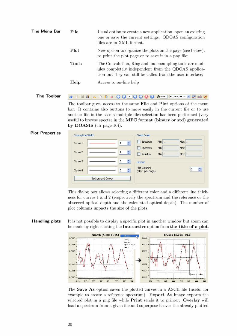
The Toolbar
The toolbar gives access to the same File and Plot options of the menubar. It contains also buttons to move easily in the current file or to useanother file in the case a multiple files selection has been performed (veryuseful to browse spectra in the MFC format (binary or std) generatedby DOASIS (cfr page 10)).
Plot Properties
This dialog box allows selecting a different color and a different line thick-ness for curves 1 and 2 (respectively the spectrum and the reference or theobserved optical depth and the calculated optical depth). The number ofplot columns impacts the size of the plots.
Handling plots It is not possible to display a specific plot in another window but zoom canbe made by right-clicking the Interactive option from the title of a plot.
The Save As option saves the plotted curves in a ASCII file (useful forexample to create a reference spectrum). Export As image exports theselected plot in a png file while Print sends it to printer. Overlay willload a spectrum from a given file and superpose it over the already plotted
20
curves but this option is not yet implemented.
2.2 The projects tree
The organisation of projects, analysis windows, spectra files and directoriesin a tree structure completed with the definition of right-click shortcutmenus at each level of the tree makes the access, manipulation and confi-guration of all these objects very easy.
Raw Spectra Spectra to analyze have to be inserted under this projects tree node. In-dividual files and complete directories structures are accepted. The “NewFolder” option allows organizing spectra files and directories within a user-defined catalog (folder that is not physically present on the disk). Thefollowing actions can be performed from any node:
Browse Spectra browses spectra in the selected file(s);
Run Analysis analyses spectra using the configuration of theproject and analysis windows; this step includesthe correction of the wavelength calibration ofthe reference spectrum if it has been requestedin the configuration of the analysis windows;
Run Calibration uses the options defined in the Calibrationpage of Projects properties (see page 67) toapply it on spectra.
ExportData/Spectra
browses spectra and saves the selected fields inASCII . If only data on records are exported,the format is the same as QDOAS output files(see Annex, page 111); otherwise, spectra aresaved in Column extended format (see An-nex, page 105)
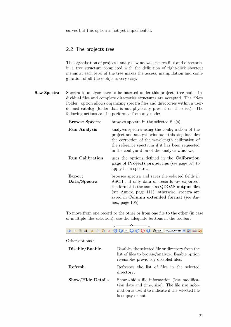
To move from one record to the other or from one file to the other (in caseof multiple files selection), use the adequate buttons in the toolbar:
Other options :
Disable/Enable Disables the selected file or directory from thelist of files to browse/analyze. Enable optionre-enables previously disabled files.
Refresh Refreshes the list of files in the selecteddirectory;
Show/Hide Details Shows/hides file information (last modifica-tion date and time, size). The file size infor-mation is useful to indicate if the selected fileis empty or not.
21
Analysis windows A project can include several spectral analysis windows. A specific analysiswindow can be disabled in order not to process it without removing it fromthe list. The View Cross Sections option is useful to check that therequested cross sections files exist.
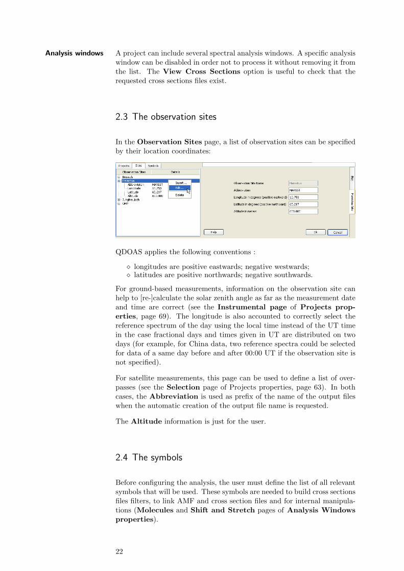
2.3 The observation sites
In the Observation Sites page, a list of observation sites can be specifiedby their location coordinates:
QDOAS applies the following conventions :
� longitudes are positive eastwards; negative westwards;� latitudes are positive northwards; negative southwards.
For ground-based measurements, information on the observation site canhelp to [re-]calculate the solar zenith angle as far as the measurement dateand time are correct (see the Instrumental page of Projects prop-erties, page 69). The longitude is also accounted to correctly select thereference spectrum of the day using the local time instead of the UT timein the case fractional days and times given in UT are distributed on twodays (for example, for China data, two reference spectra could be selectedfor data of a same day before and after 00:00 UT if the observation site isnot specified).
For satellite measurements, this page can be used to define a list of over-passes (see the Selection page of Projects properties, page 63). In bothcases, the Abbreviation is used as prefix of the name of the output fileswhen the automatic creation of the output file name is requested.
The Altitude information is just for the user.
2.4 The symbols
Before configuring the analysis, the user must define the list of all relevantsymbols that will be used. These symbols are needed to build cross sectionsfiles filters, to link AMF and cross section files and for internal manipula-tions (Molecules and Shift and Stretch pages of Analysis Windowsproperties).
22

Cross sections symbols can be completed with a short description. Thedeletion of a symbol is possible only if this symbol is not used in theconfiguration of a project or an analysis window.
23

3 Description of Algorithms
This chapter summarizes the main features of QDOAS and describes thestructure of the program and the algorithms.
3.1 Differential Optical Absorption Spectroscopy
DOAS is a widely used inversion method for the retrieval of atmospherictrace gas abundances from multi-wavelength light measurements. It usesthe structured absorption of many trace gases in the UV, visible and near-infrared spectral ranges. The DOAS method was originally developed forground-based measurements (Platt [18]; Platt and Stutz [19]) and has beensuccessfully adapted to nadir measurements from UV-Vis space-borne spec-trometers (Gottwald et al. [10]). It relies on the application of the Beer-Lambert law to the whole atmosphere in a limited range of wavelengths.
The Beer-Lambert law states that the radiant intensity traversing a homo-geneous medium decreases exponentially with the product of the extinctioncoefficient and the path length. Applying this law to the atmosphere, weobtain
I(λ) = I0(λ) exp
− n∑j=1
Sj(λ)cj
, (3.1)
where
I0 is the spectrum at the top of the atmosphere, without extinction;
I is the measured spectrum after extinction in the atmosphere;
Sj is the absorption cross section of the species j, with wavelength de-pendent structures [cm2/molec.];
cj is the column density of the species j [molec./cm2].
The logarithm of the ratio of the spectrum I0 (also called the control spec-trum) and the measured spectrum I is denoted optical density (or opticalthickness) τ
τ ≡ ln
(I0(λ)
I(λ)
)=
n∑j=1
Sj(λ)cj . (3.2)
The key idea of the DOAS method is to separate broad and narrow bandspectral structures of the absorption spectra in order to isolate the narrowtrace gas absorption features. In order to do this, some approximations aremade:
25

1. In the case where the photon path is not defined (scattered lightmeasurements), the mean path followed by the photons through theatmosphere up to the instrument is considered;
2. The absorption cross sections are supposed to be independent of tem-perature and pressure, which allows us to introduce the concept ofSlant Column Densities (SCDs);
3. Broadband variations, such as loss and gain from scattering and re-flections by clouds and/or at the earth surface, are approximated bya common low order polynomial.
Molecular absorption cross sections are fitted to the logarithm of the ratio ofthe measured spectrum and the reference spectrum (i.e. an extraterrestrialirradiance spectrum for satellite measurements, or a spectrum measuredaround the local noon when the light path is minimum for ground-basedmeasurements). The resulting fit coefficients are the integrated number ofmolecules per unit area along the atmospheric light path for each trace gas,the differential SCD. The slant column depends on the observation geom-etry, the position of the sun and also on parameters such as the presenceof clouds, aerosol load and surface reflectance.
3.2 DOAS retrieval
DOAS fitting In the DOAS analysis, high frequency spectral structures of the variousabsorbing species are used to resolve the corresponding contributions tothe measured optical density. This is achieved using a least squares fittingprocedure for the differential slant column densities of the various species.Large band contributions to the atmospheric attenuation (Rayleigh andMie scattering) are accounted for by including a low order polynomialP (λ) =
∑bkλ
k in the fit. Other effects, such as the Ring effect or in-strument undersampling can be treated as pseudo-absorbers.
According to eq. (3.2), the DOAS retrieval is a linear problem. This lin-earity is unfortunately broken down by the need to account for additionaleffects, namely:
1. small wavelength shifts ∆(λ) between I and I0 spectra must be cor-rected using appropriate shift and stretch parameters;
2. possible instrumental and/or atmospheric stray light or residual darkcurrent signal require the introduction of an offset parameter.
Including these necessary non-linear corrections and the polynomial com-ponent P (λ), we obtain the modified equation
ln
(I(λ−∆(λ))− offset(λ)
I0(λ)
)+
n∑j=1
Sj(λ)cj + P (λ) = 0 . (3.3)
Marquardt-LevenbergAlgorithm
The SCDs cj can be retrieved by performing a least squares fit of themeasurement data to equation (3.3). Due to the shift, stretch and offsetparameters, this is a non-linear least squares problem, which can typi-cally be solved using a Marquardt-Levenberg (M-L) algorithm (see Mar-quardt [16]; Bevington [3]). Starting from given initial values, this algo-rithm searches the parameter space using a combination of Gauss-Newton
26

and gradient descent steps. The M-L algorithm is an efficient minimizationalgorithm for a wide range of non-linear functions, but it may converge to alocal minimum if the initial values are too far from the global minimum. InQDOAS, this problem can occur during the wavelength calibration, whenthe initial calibration is not accurate enough (see Calibration problems insection C.2 of the appendix).
In QDOAS, the M-L algorithm is used to find the set of parameters thatminimizes the weighted1 sum of squares
F (~α) =1
2
M∑i=1
(f i(~α)
σi
)2
=1
2
M∑i=1
(ln(Ii(~a)) +
∑nj=1 S
ijcj +∑d
k=0 bk(λi)k − ln(Ii0)
σi
)2
, (3.4)
where
~α = (~a,~b,~c) is the vector containing all fitted parameters;
~a is the set of parameters describing the shift, stretch and offset of themeasured spectrum;
bk, k = 1, . . . , d are the fitted polynomial coefficients;
cj , j = 1, . . . , n are the fitted SCDs;
λi, i = 1, . . . ,M is the wavelength grid of the reference spectrum I0, cali-brated with respect to a high resolution solar spectrum (see section3.3).
Ii(~a) is the measured spectrum, including shift, stretch and offset correc-tions, interpolated at wavelength λi;
Sij is the absorption cross section of absorber species j, as measured in alaboratory, interpolated at wavelength λi;
Ii0 is the reference spectrum at wavelength λi and
σi is the standard error on the measurement at wavelength λi.
In each iteration, the fitting algorithm will choose new values for the pa-rameters using the Marquardt-Levenberg algorithm, and recompute thesum of squares F . The algorithm assumes that it has converged to a so-lution when the difference between two succeeding values of F is smallerthan a fixed small number ε. The convergence criterion ε can be chosen bythe user (see Convergence Criterion in section 5.1).
For a given value of the non-linear parameters ~a, the determination of theparameters cj and the polynomial coefficients bk is a linear least squaresproblem. Explicitly, we can rewrite equation (3.4) as
F =1
2
M∑i=1
(ln(Ii(~a)/Ii0) + (A · ~x)i
σi
)2
, (3.5)
1Weighting the residuals by the instrumental errors σi is optional in QDOAS. Whenno measurement uncertainties are used (or no error estimates are available), all un-certainties in equation (3.4) are set to σi = 1, giving all measurement points equalweight in the fit. See analysis properties in section 5.1
27

where the matrix A contains the polynomial basis (λi)k, k = 0, . . . , d and
the absorption cross sections Sij , j = 1, . . . , n and ~x represents the com-bined linear parameters ~b and ~c:
Ail =(
(λi)d Sij
), (3.6)
~x =
(~b~c
). (3.7)
This fact is exploited in QDOAS to limit the parameter space of the M-L algorithm to the non-linear parameters: once a new set of values ~a′
for the non-linear parameters is chosen, the linear parameters bk and cjare updated using a linear least squares algorithm, minimizing the sum ofsquares (3.4) for the given values of the non-linear parameters.
In QDOAS, the linear least squares problem is solved using the QR decom-position of the matrix A defined in equation (3.6).
QDOAS can include further parameters in the fits (3.4), which we omittedfrom the previous description for the purpose of clarity. Such parametersinclude the width of the instrument’s slit function and wavelength shifts inthe reference absorption cross sections Sj(λ). Mathematically, they playthe same role as the shift, stretch and offset parameters ~a. Section 5.3describes the available fitting options in QDOAS and their configuration.
Intensity fitting QDOAS also supports the so-called intensity fitting (or direct fitting) methodwhere measured intensities are directly fitted instead of their logarithms.The equation used in the least squares fitting procedure is then
I(λ−∆(λ))− offset(λ)
I0(λ)− P exp(−
n∑j=1
Sjcj) = 0 , (3.8)
This method involves a decomposition of equation (3.8) in its linear andnon-linear parts: column densities are fitted non-linearly, but the polyno-mial, which is taken out of the exponential function using a Taylor expan-sion, and offset are linear parameters.
Intensity fitting is sometimes preferred to optical density fitting, for ex-ample when a poor signal leads to numerical problems when taking thelogarithms of the intensity ratio.
Errors On Slant ColumnDensities
Uncertainties on the retrieved slant columns cj depend on:
� the sensitivity of the sum of squares F (3.4) with respect to variationsof the fitted parameters around the minimum and
� the noise on the measurements.
Formally, the covariance matrix of the fitted parameters of a least squaresestimate may be estimated by the inverse of the Hessian of the sum ofsquares F , evaluated at the fitted values of the parameters
Σ~α = H−1 , (3.9)
where H is given by
Hkl =∂2F
∂αk∂αl. (3.10)
28

The actual approach used to calculate H in QDOAS is different in opticaldensity fitting mode and in intensity fitting mode. In optical density fittingmode, the slant column density is fitted linearly according to equation (3.5)and we use the following expression for the covariance matrix Σ~x of theweighted linear least squares parameter estimate:
Σ~x =(ATW 2A
)−1, (3.11)
where the matrix A contains the linear components of the fit, as describedin equation (3.6) and the (M ×M) diagonal matrix W contains the mea-surement errors
Wij =1
σiif i = j . (3.12)
Equation (3.11) implies that uncertainties on estimated values of the non-linear parameters are not taken into account in the reported errors on theslant columns.
When the individual measurement errors σi are not available (or the userhas chosen not to weight the fit by the instrumental errors), the weightmatrix W is just the identity matrix. In this case, the mean squared erroron the measurements σ2 may be estimated by the reduced χ2, e.g. the sumof squares of the residuals divided by the number of degrees of freedom inthe fit
χ2 =
∑Mi=1(f i)2
M −N, (3.13)
where M is the number of wavelengths included in the fit, and N is thetotal number of fitted parameters. Equation (3.11) then becomes
Σ~x = χ2(ATA
)−1. (3.14)
In intensity fitting mode, the slant column densities are determined usingnon-linear least squares fitting, and the Hessian is approximated by thesquare of the Jacobian of the fitting functions f i
Hkl 'M∑j=1
∂f j
∂αk
∂f j
∂αl
1
(σj)2. (3.15)
This implies that, in intensity fitting mode, uncertainties on the linearparameters are not taken in to account in the reported slant column errors.As in the linear case, when the instrumental errors are not used or notavailable, the σj in equation (3.15) are replaced by 1, and the measurementerror is approximated using the reduced χ2 of the fit instead. Equation (3.9)then becomes
Σ~α = χ2H−1 . (3.16)
Limitations The estimates for the uncertainties of the fitted parameters rely on thestatistical model used for the DOAS retrieval. The model assumes thatthe errors on the measurements at each frequency are independent andnormally distributed. When measurement errors are correlated or containsystematic components, or in case of fitting errors such as a wrong fit forshift and stretch parameters, or relevant absorbers that are not includedin the fit, the uncertainties calculated by QDOAS will underestimate the
29
true error on the slant column density. Remaining residual structures afterthe fit, or a value of χ2 � 1 when measurement errors σi are taken intoaccount, are an indication of such a bad fit. A discussion can be foundin Stutz and Platt [24].
We also note that the errors in QDOAS do not take into account theuncertainties on the cross sections. A way to achieve this is given in Theyset al. [25].
3.3 Wavelength calibration
The quality of the retrieval fit strongly depends on a perfect alignment be-tween the spectrum to analyze, the reference spectrum and the cross sec-tions. The wavelength-pixels relation (see Platt and Stutz [19]) of the refer-ence spectrum, previously determined in laboratory using a lamp spectrumcan be corrected using a procedure based on the alignment of the Fraun-hofer structures of the reference spectrum I0 with those of an accuratelycalibrated high-resolution solar reference atlas, degraded at the resolutionof the instrument, i.e. convolved with the instrumental slit function. Thereference atlas used for this purpose is usually the Chance and Kurucz [8]spectrum.
During the calibration process, the instrumental slit function can also becharacterized by repeatedly convolving the highly resolved solar atlas withthe slit function and adjusting the parameters until the best match withthe reference spectrum is found. QDOAS allows fitting the parameters ofdifferent line shapes, as well as their wavelength dependence. This is usefulwhen the slit function provided with the instrument is not described pre-cisely enough in the wavelength interval used for the retrieval. In the sameway, to account for the moderate resolution of satellite or ground-basedinstruments (about a few tenths of a nanometer), the absorption cross sec-tions of the trace gases have to be convolved with the instrumental slitfunction (and interpolated on the final I0 wavelength grid). A good knowl-edge of the instrumental slit function and its potential wavelength variationis important to avoid systematic errors in the retrieved slant columns dueto spectral shape mismatch between the reference and atmospheric spec-tra [26].
Fit of shift and stretch Shift and stretch (see Shift on page 33) can be taken into account in thewavelength calibration scheme. To this end, the spectral interval is dividedinto a number of sub-intervals. By default, QDOAS will split the completecalibration interval into equally sized disjoint sub-intervals, but more ad-vanced options are available, too (see Calibration Windows on page 89).The fitting algorithm used for the DOAS retrieval is then applied in eachsub-interval to fit the measured intensities to those of the high-resolutionsolar spectrum, according to the equation
I0(λ) = IS(λ−∆i − ai(λ− λc,i)) exp(−m∑j=1
Sjcj) , (3.17)
where IS is the solar spectrum convolved at the resolution of the instru-ment, ∆i is a fitted constant shift in sub-interval i, λc,i the central wave-
30

length of sub-interval i, ai the interval’s fitted stretch factor, and the cjare optional absorber coefficients accounting for possible light absorptionin the reference spectrum I0. Typically, the calibration uses more then onesub-interval, and we fit a polynomial through the pairs (λc,i,∆i) in orderto reconstruct an accurate wavelength calibration ∆(λ) for the completeanalysis interval. When the calibration is set to use only a single interval,the shift and stretch values from this interval are used to calculate theoptimized wavelength grid for the analysis.
Several tests may be needed to determine the best configuration. Onehas to find the right compromise between using enough sub-intervals torepresent the wavelength variation of the shift, and having enough spectralinformation in each sub-window. The interval calibration should cover allanalysis spectral windows.
The algorithm can take into account molecular absorption and offset cor-rection. In order to help the algorithm to converge to the correct solution,it is important to start with a preliminary wavelength grid close enough tothe real one and to limit the number of fitting parameters (for example byfixing the value of some parameters, typically the concentration of the fittedmolecules after a first estimation). Another option to help the algorithmconverge is to determine the initial shift by testing for correlation:
Calculation of thepreshift
When the wavelength shift between the high-resolution solar atlas andthe initial calibration of the reference spectrum is too large, the fittingalgorithm used in the calibration procedure may not converge to the propervalue. If you find that this is the case, you can choose to perform an extra“preshift” calculation. With this option, QDOAS performs the followingextra steps before running the wavelength calibration algorithm:
1. The high-resolution solar spectrum is degraded to instrument resolu-tion using the chosen slit function settings. If slit function parametersare also fit during the calibration, their initial values are used for thisstep.
2. The convolved solar spectrum and the reference spectrum are smoothedand normalized, with an averaging bandwidth of about 5nm.
3. Using the Nelder-Mead optimization algorithm, QDOAS determinesthe shift value resulting in the highest correlation between the refer-ence and high-resolution solar spectrum.
After this preshift step, QDOAS performs the regular wavelength calibra-tion on the original spectra, using the preshift value as the initial value forthe calibration shift in each sub-interval.
Ref2/Ref1 Alignment If two reference spectra are given (see section 5.1 and figure 5.18), thewavelength calibration described in the previous section is applied to thefirst one. The shift between both reference spectra is then determined usinga least squares fit. This shift is then applied to the reference absorptioncross sections in order to align them on the second reference spectrum. Themeasured spectra are then analyzed with respect to the second referencespectrum.
31
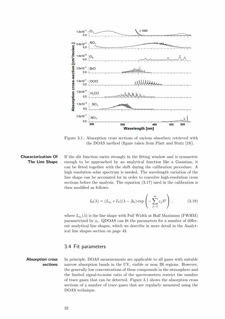
Figure 3.1.: Absorption cross sections of various absorbers retrieved withthe DOAS method (figure taken from Platt and Stutz [19]).
Characterization OfThe Line Shape
If the slit function varies strongly in the fitting window and is symmetricenough to be approached by an analytical function like a Gaussian, itcan be fitted together with the shift during the calibration procedure. Ahigh resolution solar spectrum is needed. The wavelength variation of theline shape can be accounted for in order to convolve high-resolution crosssections before the analysis. The equation (3.17) used in the calibration isthen modified as follows:
I0(λ) = (Lai ∗ IS)(λ−∆i) exp
− m∑j=1
cjSj
, (3.18)
where Lai(λ) is the line shape with Full Width at Half Maximum (FWHM)parametrized by ai. QDOAS can fit the parameters for a number of differ-ent analytical line shapes, which we describe in more detail in the Analyt-ical line shapes section on page 43.
3.4 Fit parameters
Absorption crosssections
In principle, DOAS measurements are applicable to all gases with suitablenarrow absorption bands in the UV, visible or near IR regions. However,the generally low concentrations of these compounds in the atmosphere andthe limited signal-to-noise ratio of the spectrometers restrict the numberof trace gases that can be detected. Figure 3.1 shows the absorption crosssections of a number of trace gases that are regularly measured using theDOAS technique.
32
Many spectral regions contain a large number of interfering absorbers. Inprinciple, because of their unique spectral structure, a separation of theabsorption is possible. However, correlations between absorber cross sec-tions sometimes lead to systematic biases in the retrieved slant columns. Ingeneral, the correlation between cross sections decreases if the wavelengthinterval is extended, but doing so is at odds with the assumption that a sin-gle effective light path for the entire wavelength interval is defined, leadingto systematic misfit effects that may also introduce biases in the retrievedslant columns. To optimize DOAS retrieval settings, a trade-off has tobe found between these effects. A basic limitation of the classical DOAStechnique is the assumption that the atmosphere is optically thin in thewavelength region of interest. At shorter wavelengths, the usable spectralrange of DOAS is limited by rapidly increasing Rayleigh scattering and O3
absorption. In addition, ‘line-absorbers’ such as H2O, O2, CO, CO2 andCH4 usually cannot be retrieved precisely by standard DOAS algorithmsbecause their strong absorption also depends on pressure and temperature.
The selection of the spectral analysis window determines which absorbershave to be included in the fitting procedure. The pressure dependence ofabsorption cross sections can be neglected in UV-Visible region. However,the temperature dependence of cross sections can be significant (for exam-ple that of O3 and NO2). This can be corrected in a first approximation byintroducing correction factors during the AMF calculation [4] or, assuminga linear dependence on temperature, by fitting two absorption cross sec-tions at different temperatures as described in Van Roozendael et al. [26].
Shift Before analysis, absorption cross sections are interpolated on the final gridof the reference spectrum which may be determined by the program itself(automatic reference selection mode). Moreover, shift and stretch param-eters can be fitted during the processing of a spectrum in order to obtainthe best match of the absorption structures.
Interpolation/Convolution Cross sections can be pre-convolved and interpolated2 on an appropriatewavelength grid prior to the analysis. However, the direct use of high-resolution cross sections which can be convolved in real-time with a prede-fined slit function or with the slit function determined by the wavelengthcalibration procedure, is more convenient.
Differential cross sections The aim of calculating differential absorption cross sections is to separatenarrow spectral features from unstructured absorption not useful in theDOAS method. Figure 3.2 gives an illustration.
Differential cross sections can be calculated by orthonormalization with re-spect to an orthogonal set formed with the low order component vectors(usually a base of order 2 or 3) of the polynomial. The vectors are orthog-onalized using the Gram-Schmidt algorithm. This method gives also thepossibility to separate the spectral structures of temperature dependentcross sections by mutually orthogonalizing them. Differential cross sec-tions can alternatively be obtained by high-pass filtering: a filter is appliediteratively on the cross section and the resulting cross section is subtracted
2By default, QDOAS uses cubic spline interpolation.
33

Figure 3.2.: Cross section O3 and optical thickness τ are separated into anarrow (O′3 and τ ′) and a broad band part (O3p and τp) by anadequate filtering procedure.
from the original one. High-pass filtering is presently only supported inoptical density fitting mode (DOAS mode). Note that it is not necessaryto calculate differential cross sections when the baseline is around 0 suchas for H2O, O4 or H2CO.
Low-pass filtering Low-pass filters can be applied to both spectra and absorption cross sec-tions. A large choice of filters is proposed (see ‘Filtering Page’, section5.1).
Wavelength-dependent AMF Absorption cross sections can be replaced by geometrically corrected crosssections that take into account the wavelength dependency of the AMF.The correction is based on the equation
ln(I0)− ln(I) = S(λ)AMF(λ,SZA) , (3.19)
where AMF(λ, SZA) is the AMF calculated for a given wavelength λ anda given Solar Zenith Angle (SZA).
Polynomial In the DOAS technique, absorption cross sections of the considered mole-cules are highly structured, while scattering by molecules and particles(Rayleigh and Mie scattering), as well as reflection at the surface, havebroadband dependencies that can be approximated by a low order polyno-mial. In QDOAS, polynomials up to degree 5 can be fitted. The low ordercomponents of the polynomial can be used to calculate differential crosssections when this is preferred to high-pass filtering.
Shift and Stretch Shift and stretch parameters allow to correct possible misalignment be-tween the various wavelength-dependent quantities involved in the dataevaluation (i.e. measured and reference spectra as well as absorption crosssections). Shift and stretch parameters may be fitted or simply applied toany wavelength-dependent quantity, according to the equation
∆λ = a+ b(λ− λ0) + c(λ− λ0)2 , (3.20)
where λ is the wavelength according to the original calibration and λ0 isthe center wavelength of the current spectral range. The parameters a,b
34
and c describe the offset and the first and second order stretch applied toλ.
Offset Correction An ideal spectrometer in an ideal atmosphere would measure the part of thesunlight that has been elastically scattered by air molecules and particles.In a real experiment, however, a number of possible additional sourcesmay contribute to the measured intensity, adding an “offset” to the idealRayleigh/Mie contribution. In addition to the Ring effect, which is, toa first approximation, a natural source of offset, one must also accountfor instrumental sources of offset, such as stray light in the spectrometerand dark current of the detector. The offset component in equation (3.3)accounts for these effects. QDOAS models the offset using a polynomial
offset(λ) = (a+ b(λ− λ0) + c(λ− λ0)2)I , (3.21)
where λ0 is the center wavelength of the spectral analysis window, I is theaverage intensity and a, b and c are fitted parameters.
Due to the normalization by I, the offset values can be easily interpretedrelatively to the absolute intensity of the spectrum (percent offset). InDOAS, the offset is usually fitted as a non-linear parameter. Sometimes,this could lead to numerical errors in the evaluation of the logarithm, typi-cally in the near UV region where the level of the signal is very low. In thiscase, we can fit the offset as a linear parameter. Expanding the left-handside of equation (3.3) to first order, we obtain
ln(I(λ−∆(λ))) = ln(I0(λ))− τ(λ) +offset(λ)
I(λ+ ∆λ). (3.22)
Ring Effect Because of Rotational Raman Scattering (RRS), a small fraction of theincident photons undergo a wavelength change of a few nanometres, i.e.a part of the scattering is inelastic. This causes an intensity loss at theirincident wavelength and a gain at the neighbouring wavelengths to whichthey are redistributed. RRS causes the so-called “filling-in” of Fraunhoferlines, which have a slightly different shape in the earthshine radiance thanin the direct solar light. This effect was first discovered by Grainger andRing [11] and is referred to as the Ring effect. The atmospheric absorp-tion lines are also broadened by RRS events occurring after absorption(molecular Ring effect). Although RRS accounts for only a few percentof the measured intensity, it significantly affects DOAS measurements ofscattered radiation since typical trace gas absorptions are of the order of apercent or less. If not properly corrected, the Ring effect produces stronglystructured residuals in the differential optical density, due to the fact thatFraunhofer lines do not cancel perfectly between I and I0. Especially inthe UV spectral range, the remaining spectral structures can by far exceedthe structures of weak atmospheric absorbers.
Usually the Ring effect is taken into account by including an additional ‘ab-sorber’ in the DOAS fit. Ring cross sections SRing(λ) can be measured [23]or calculated [9]. The Ring effect can be approximated using the followingdevelopment for an optically thin atmosphere [28; 26]:
One can consider that in any scattered light observation, the light detectedby the satellite instrument (Imeas) is the sum of elastic and inelastic scat-
35

tering processes:
Imeas = Ielastic + IRRS = I0e−τ + IRRS . (3.23)
To analyze a measured spectrum, the logarithm of Imeas is taken. SinceIRRS is very small compared to Ielastic, the logarithm can be approximatedby the first two terms of the Taylor expansion:
ln(Imeas) = ln(Ielastic) +IRRS
Ielastic= ln I0 − τ +
IRRS
Ielastic. (3.24)
The last term IRRS/Ielastic is the Ring term which can be approximatedby the product of a Ring coefficient αRing and a Ring cross section SRing.αRing can be fitted together with other absorbers in the DOAS procedure.
A good approximation of the Ring cross section can be obtained fromcalculation of a source term IRaman
0 for Raman scattering derived by sim-ple convolution of the solar spectrum with Raman cross sections, i.e withcalculated N2 and O2 RRS cross sections. The term IRRS/Ielastic in equa-tion (3.24) is then substituted by αRingSRing (where SRing = IRaman
0 /I0),assuming that the molecular Ring effect can be neglected [9]. The QDOASRing tool calculates a Ring cross section according to this approach [28].The normalization of the Raman spectrum is optional.
UndersamplingCorrection
The undersampling is a well-known problem of GOME [7]. It arises fromthe poor sampling ratio of the GOME instrument, which results in a lossof spectral information when interpolating earthshine spectra during theDOAS fitting process. Undersampling is only a major problem when thesampling ratio is close to 1. In the case of GOME, this ratio is estimatedat 0.16/0.112=1.43 at 340 nm.
The undersampling artifacts can be corrected using an ad-hoc cross sectionobtained by simulating the effect based on a high-resolution solar refer-ence [7]. This cross section is fitted as a linear parameter, in both intensityfitting and in optical density fitting modes. The procedure to calculate thecorrection differs slightly between the two fitting modes:
In intensity fitting mode, oversampled and undersampled spectra are cal-culated as follows:
U(λ+ ∆) = over(λ+ ∆)− under(∆)(λ) , (3.25)
where over(λ + ∆) is a high-resolution solar spectrum convolved on itsoriginal grid and interpolated on the final grid λ + ∆ and under(∆)(λ)is a high-resolution solar spectrum convolved on grid λ and subsequentlyinterpolated on the final grid λ+ ∆.
Residuals are improved by adding a “second phase” of undersampling
U2(λ) = over(λ)− under(∆)(λ) . (3.26)
In optical density fitting, we fit the logarithm of the ratio of the measuredintensities. We therefore use the corresponding equations
U(λ+ ∆) = ln
(over(λ+ ∆)
under(∆)(λ)
), (3.27)
U2(λ) = ln
(over(λ)
under(∆)(λ)
). (3.28)
36
Calculated Measured
Residual Rod
Cross sections Sj · cj Sj · cj +Rod
Polynomial P P +Rod
Offset O O +Rod
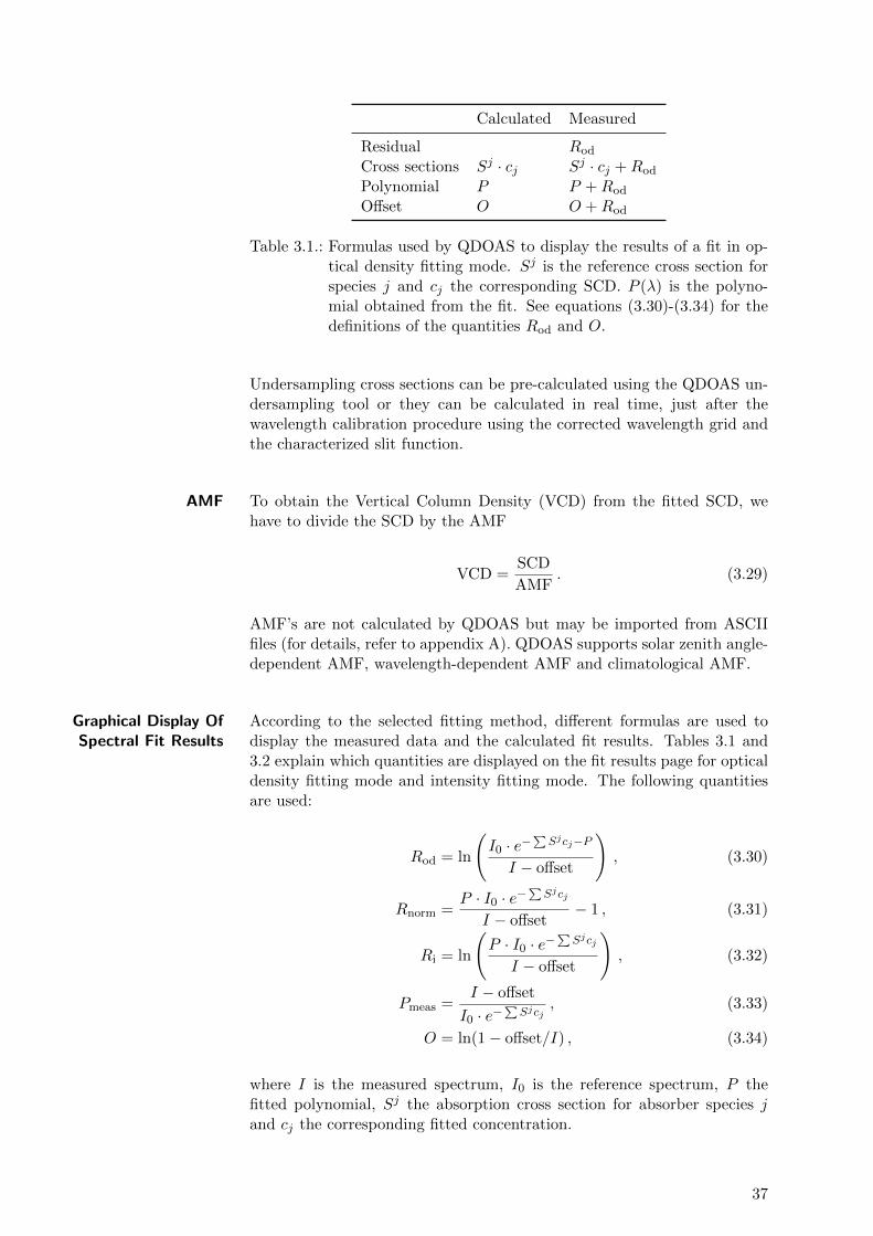
Table 3.1.: Formulas used by QDOAS to display the results of a fit in op-tical density fitting mode. Sj is the reference cross section forspecies j and cj the corresponding SCD. P (λ) is the polyno-mial obtained from the fit. See equations (3.30)-(3.34) for thedefinitions of the quantities Rod and O.
Undersampling cross sections can be pre-calculated using the QDOAS un-dersampling tool or they can be calculated in real time, just after thewavelength calibration procedure using the corrected wavelength grid andthe characterized slit function.
AMF To obtain the Vertical Column Density (VCD) from the fitted SCD, wehave to divide the SCD by the AMF
VCD =SCD
AMF. (3.29)
AMF’s are not calculated by QDOAS but may be imported from ASCIIfiles (for details, refer to appendix A). QDOAS supports solar zenith angle-dependent AMF, wavelength-dependent AMF and climatological AMF.
Graphical Display OfSpectral Fit Results
According to the selected fitting method, different formulas are used todisplay the measured data and the calculated fit results. Tables 3.1 and3.2 explain which quantities are displayed on the fit results page for opticaldensity fitting mode and intensity fitting mode. The following quantitiesare used:
Rod = ln
(I0 · e−
∑Sjcj−P
I − offset
), (3.30)
Rnorm =P · I0 · e−
∑Sjcj
I − offset− 1 , (3.31)
Ri = ln
(P · I0 · e−
∑Sjcj
I − offset
), (3.32)
Pmeas =I − offset
I0 · e−∑Sjcj
, (3.33)
O = ln(1− offset/I) , (3.34)
where I is the measured spectrum, I0 is the reference spectrum, P thefitted polynomial, Sj the absorption cross section for absorber species jand cj the corresponding fitted concentration.
37
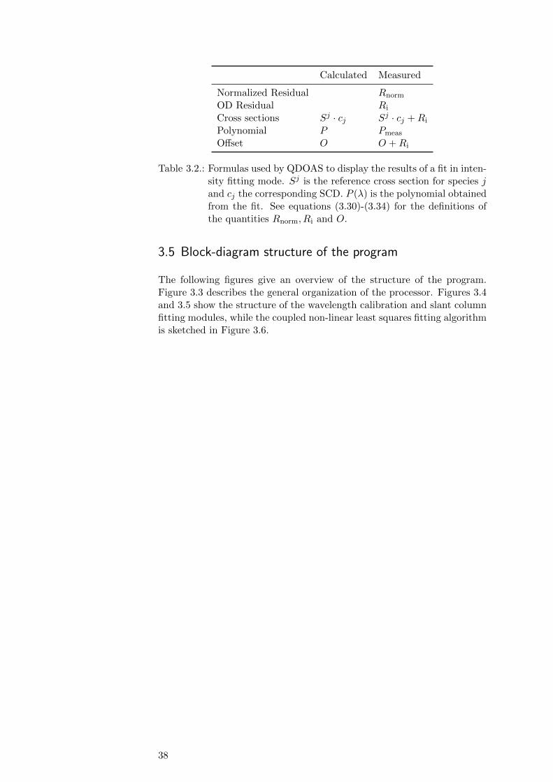
Calculated Measured
Normalized Residual Rnorm
OD Residual Ri
Cross sections Sj · cj Sj · cj +Ri
Polynomial P Pmeas
Offset O O +Ri
Table 3.2.: Formulas used by QDOAS to display the results of a fit in inten-sity fitting mode. Sj is the reference cross section for species jand cj the corresponding SCD. P (λ) is the polynomial obtainedfrom the fit. See equations (3.30)-(3.34) for the definitions ofthe quantities Rnorm, Ri and O.
3.5 Block-diagram structure of the program
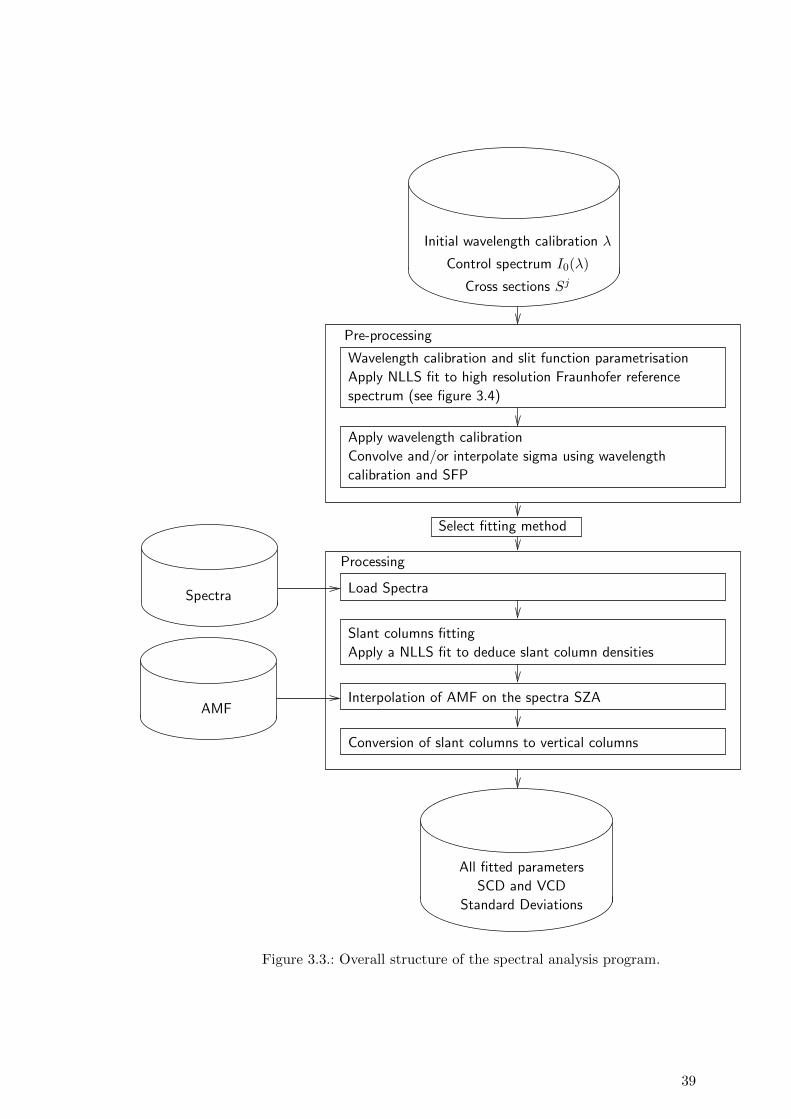
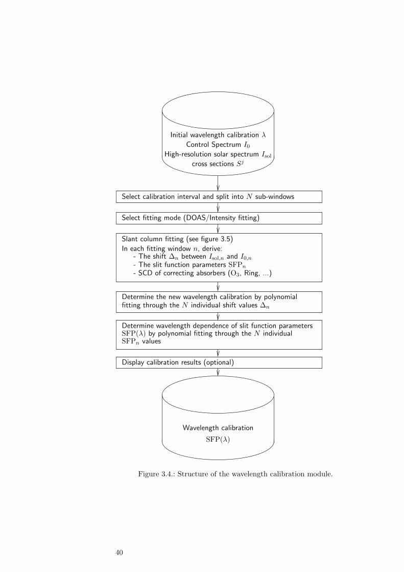
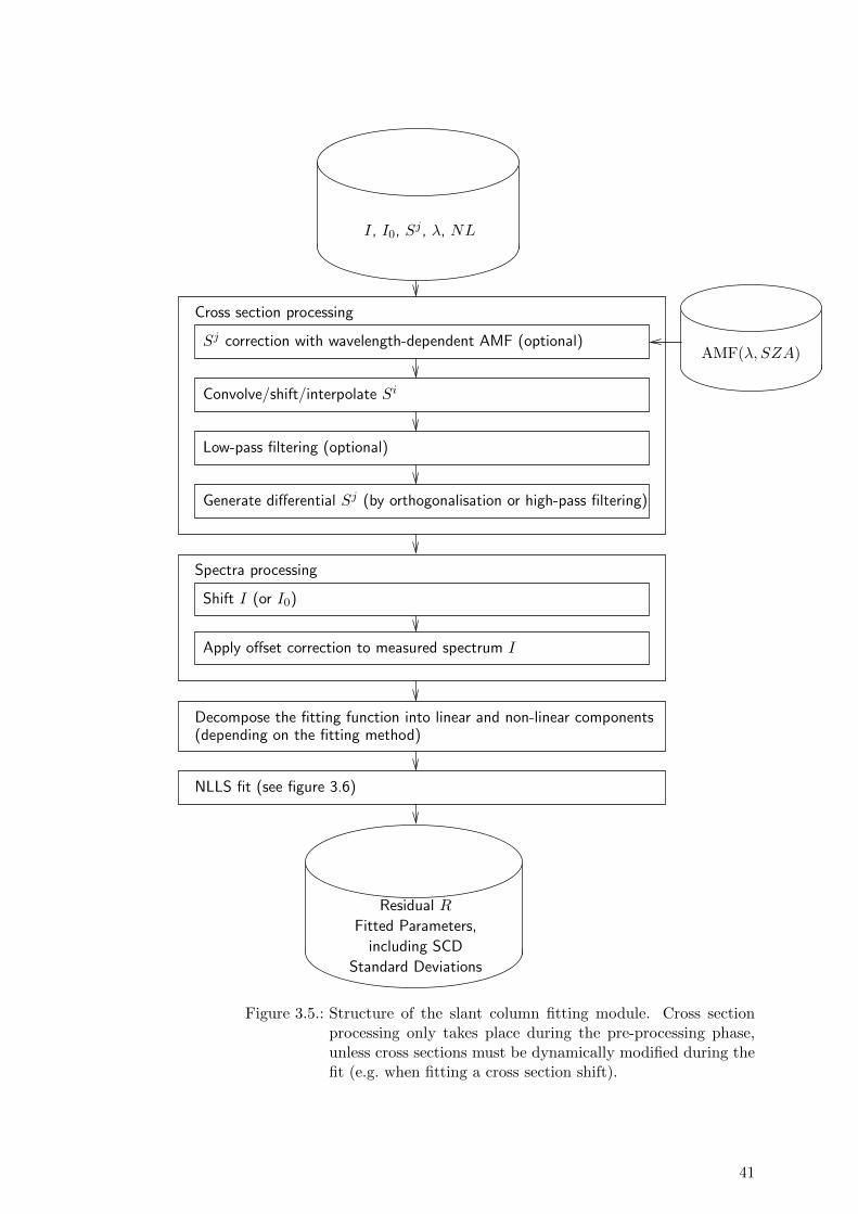
The following figures give an overview of the structure of the program.Figure 3.3 describes the general organization of the processor. Figures 3.4and 3.5 show the structure of the wavelength calibration and slant columnfitting modules, while the coupled non-linear least squares fitting algorithmis sketched in Figure 3.6.
38
Spectra
AMFInterpolation of AMF on the spectra SZA
Apply a NLLS fit to deduce slant column densities
Slant columns fitting
Load Spectra
Conversion of slant columns to vertical columns
Apply wavelength calibration
calibration and SFP
Convolve and/or interpolate sigma using wavelength
spectrum (see figure 3.4)
Apply NLLS fit to high resolution Fraunhofer reference
Wavelength calibration and slit function parametrisation
Select fitting method
Initial wavelength calibration λ
Control spectrum I0(λ)
Cross sections Sj
All fitted parameters
SCD and VCD
Standard Deviations
Processing
Pre-processing
Figure 3.3.: Overall structure of the spectral analysis program.
39
Display calibration results (optional)
SFP(λ)
Wavelength calibration
Select calibration interval and split into N sub-windows
Select fitting mode (DOAS/Intensity fitting)
In each fitting window n, derive:- The shift ∆n between Isol,n and I0,n
- The slit function parameters SFPn- SCD of correcting absorbers (O3, Ring, ...)
Determine the new wavelength calibration by polynomialfitting through the N individual shift values ∆n
Determine wavelength dependence of slit function parametersSFP(λ) by polynomial fitting through the N individual
Slant column fitting (see figure 3.5)
SFPn values
Initial wavelength calibration λ
Control Spectrum I0
High-resolution solar spectrum Isol
cross sections Sj
Figure 3.4.: Structure of the wavelength calibration module.
40
I, I0, Sj , λ, NL
Low-pass filtering (optional)
Generate differential Sj (by orthogonalisation or high-pass filtering)
Convolve/shift/interpolate Si
Shift I (or I0)
Apply offset correction to measured spectrum I
Fitted Parameters,
Standard Deviations
including SCD
Residual R
AMF(λ, SZA)Sj correction with wavelength-dependent AMF (optional)
Cross section processing
Spectra processing
Decompose the fitting function into linear and non-linear components(depending on the fitting method)
NLLS fit (see figure 3.6)
Figure 3.5.: Structure of the slant column fitting module. Cross sectionprocessing only takes place during the pre-processing phase,unless cross sections must be dynamically modified during thefit (e.g. when fitting a cross section shift).
41

I, I0 low pass and high pass filtering (optional)
Initialization of non-linear parameters
NLLS fit
Update non-linear parameters according to Marquardt-Levenberg algorithm
LLS fitMinimize F (eq. (3.4)) for current values of non-linearparameters by solving the linear least squares problem
Fitted Parameters,
Standard Deviations
including SCD
Residual R
∆F < ε
I, I0, Sj , λ
y
n
Figure 3.6.: Structure of the non-linear least squares fitting algorithm usedin the slant column fitting module and in the wavelength cali-bration module.
42

3.6 Convolution
Definition The convolution of a spectrum I by an instrumental slit function F is givenby the integral
(F ∗ I)(λ) =
∫I(λ′)F (λ− λ′)dλ′ . (3.35)
In QDOAS, this integral is calculated using the trapezoidal rule. Theintegration interval is defined by the width of the slit function.
The three tools (Convolution, Ring and Usamp) provided in the QDOASpackage, support convolution with one of the following functions:
� the Gaussian line shape,
� the 2n-Lorentzian line shape,
� the Voigt profile,
� the error function,
� an asymmetrical Gaussian line shape,
� the super-Gaussian line shape ([2]),
� a boxcar (using Fourier Transform)
� Norton-Beer strong (using Fourier Transform)
� arbitrary line shapes provided in ASCII files.
Analytical line shapes QDOAS can calculate the Gaussian, Lorentzian, Voigt, asymmetrical Gaus-sian, super-Gaussian and error function line shapes for different values oftheir parameters. When one of these analytical line shapes is used, QDOAScan fit its parameters during the wavelength calibration procedure (see sec-tion 3.3, page 32).
In order to make the convolution algorithm faster, analytical slit functionsare pre-calculated on a suitable wavelength grid (determined in order tohave 18 pixels at FWHM) and then interpolated on the grid of the spec-trum. For Gaussian and error function line shapes, a Fast Fourier Trans-form (FFT) algorithm is used whenever possible to speed up the calculation(e.g. within the wavelength calibration procedure).
As a convention, QDOAS always requests the full width at halfmaximum (FWHM) of the line shape in the user interface. Thisparameter is represented by σ in the formulas below.
Gaussian The standard expression used to approximate instrumental slit functionsis the Gaussian function (see figure 3.7(a)). The Gaussian is the exact lineshape in the diffraction limit, i.e. in the case of an infinitely thin entranceslit. The normalized Gaussian is given by
Gσ(x) =1
a√π
exp
(−x
2
a2
), (3.36)
where a depends on the Gaussian full width at half-maximum σ as follows:
σ = 2√
ln 2a . (3.37)
43
(a) (b) (c)
(d) (e) (f)
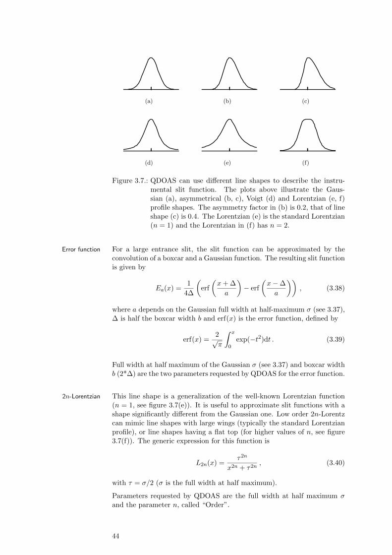
Figure 3.7.: QDOAS can use different line shapes to describe the instru-mental slit function. The plots above illustrate the Gaus-sian (a), asymmetrical (b, c), Voigt (d) and Lorentzian (e, f)profile shapes. The asymmetry factor in (b) is 0.2, that of lineshape (c) is 0.4. The Lorentzian (e) is the standard Lorentzian(n = 1) and the Lorentzian in (f) has n = 2.
Error function For a large entrance slit, the slit function can be approximated by theconvolution of a boxcar and a Gaussian function. The resulting slit functionis given by
Ea(x) =1
4∆
(erf
(x+ ∆
a
)− erf
(x−∆
a
)), (3.38)
where a depends on the Gaussian full width at half-maximum σ (see 3.37),∆ is half the boxcar width b and erf(x) is the error function, defined by
erf(x) =2√π
∫ x
0exp(−t2)dt . (3.39)
Full width at half maximum of the Gaussian σ (see 3.37) and boxcar widthb (2*∆) are the two parameters requested by QDOAS for the error function.
2n-Lorentzian This line shape is a generalization of the well-known Lorentzian function(n = 1, see figure 3.7(e)). It is useful to approximate slit functions with ashape significantly different from the Gaussian one. Low order 2n-Lorentzcan mimic line shapes with large wings (typically the standard Lorentzianprofile), or line shapes having a flat top (for higher values of n, see figure3.7(f)). The generic expression for this function is
L2n(x) =τ2n
x2n + τ2n, (3.40)
with τ = σ/2 (σ is the full width at half maximum).
Parameters requested by QDOAS are the full width at half maximum σand the parameter n, called “Order”.
44
Voigt profile The Voigt profile function (see figure 3.7(d)) is the convolution of a Gaus-sian and a Lorentzian function. This function is used in a wide rangeof contexts, and the optimization of its computation has received muchattention. The Voigt profile is usually expressed as
K(x, y) =y
π
∫ ∞−∞
exp(−t2)
(x− t)2 + y2dt , (3.41)
where x is the distance from the line center in units of Gaussian half-widthsand y is the ratio of the Lorentzian width to the Gaussion width. Numerousways have been proposed to compute the Voigt function. A rather efficientalgorithm is described by Kuntz [14].
Asymmetrical Gaussian To handle asymmetrical line shapes, QDOAS can fit an asymmetry factorin addition to the FWHM. The line shape used is a modified version of theGaussian line shape (3.36)
G′(x) =1
a√π
exp
(− x2
a2(1 + sign(x)b)2
), (3.42)
where, in addition to the FWHM σ, the asymmetry factor b is now fitted aswell. For a value of b = 0, it reduces to the ordinary Gaussian line shape.Figure 3.7(b) illustrates the line shape with an asymmetry factor of b = 0.2and 3.7(c) gives an illustration for b = 0.4.
Super Gaussian This line shape is a generalization of the Gaussian with the introduction oftwo independent parameters, w and k, determining the width and shape ofthe slit function. This line shape has been the subject of studies by SteffenBeirle from the Max-Planck Institute in Germany and summarized in arecent paper ([2]). The current implementation in QDOAS is operationalbut not optimized in terms of performance.
User-defined line shape An alternative to fit asymmetrical slit functions is to provide a line shape inan ASCII file and to apply on the grid of the line shape a stretch factor thatcan be different for each side of the line shape. The “Stretch on wavelength”file in the Convolution tool is a ASCII file with three columns : thewavelength calibration and the two values of the stretch to apply on thegrid of the line shape for each wavelength of the detector.
Lookup tables of slit functions are also accepted. This means that a lineshape is provided for different wavelengths. For a specific wavelength, aline shape is first calculated by linear 2D-interpolation in the lookup tableand the fitted stretch factors are then applied to the line shape wavelengthgrid before convolution.
Wavelengthdependency
QDOAS supports convolution with wavelength-dependent slit functions:
� Slit function files provided by the user may contain multiple columnsdescribing the shape of the slit function at various wavelengths. Thefirst line of the file should list the wavelengths for which the slit func-tion is provided. QDOAS will then generate a lookup table from theprovided slit functions, and calculate the slit function at intermediatewavelength values using linear interpolation.
45

� For analytical line shapes, the user can provide a two-column ASCIIfile containing the wavelengths and corresponding values of the pa-rameters for each requested parameter (for example, the Gaussianwidth and the boxcar width for the error function). Files with thecorrect parameter calibration can be saved from the SFP plots ob-tained after the wavelength calibration procedure.
For more details on how to compute such a convolution using QDOAS, seesection 6.1, page 95.
Correction for the SolarI0-effect
The I0-effect is due to the difference between cross sections measured inthe laboratory with a smooth light source and the atmospheric absorptionmeasured by an instrument of lower resolution with a structured solar lightsource [1]. As described in equation (3.2), the DOAS technique attemptsto isolate the atmospheric absorptions by calculating the ratio of a refer-ence spectrum I0 and a measured spectrum I. However, because the twospectra in this ratio have been filtered by the instrument function beforethe calculation of the ratio, complete removal of the Fraunhofer structurefrom the solar reference spectrum is not possible:
If the I0-effect is not accounted for, the cross sections S used in the DOASretrieval are laboratory cross sections S0 convolved with the instrumentalslit function F :
S(λ) = (F ∗ S0)(λ) =
∫S0(λ′)F (λ− λ′)dλ′ . (3.43)
The intensities measured by the spectrometer can be defined as
Imeas0 (λ) = (F ∗ I0)(λ) , (3.44)
Imeas(λ) = (F ∗ I)(λ) = (F ∗ I0 exp(−S0 · c)) (λ) . (3.45)
Taking into account the instrumental function F , equation (3.2) becomes:
τ = lnImeas
0 (λ)
Imeas(λ)= ln
(F ∗ I0)(λ)
(F ∗ I0 exp(−S0 · c))(λ)(3.46)
' c · (F ∗ S0)(λ) . (3.47)
Thus, the fitting of convolved laboratory cross sections to the optical depthmeasured by a low resolving instrument relies on an approximation. Theerror induced by this approximation depends on the absorption strengthand the relation between the width of the slit function and the width of thespectral structures in the light source I0 and the cross section S0. For mostof the atmospheric absorbers the I0-effect is negligible but in some cases,the approximation (3.47) is not accurate enough. This is particularly thecase for strong atmospheric absorbers such as O3.
This effect may be dealt with to a good approximation by correcting thelaboratory cross sections with the solar Fraunhofer spectrum: for a par-ticular absorber, a highly resolved solar spectrum I0(λ) and a simulatedabsorption spectrum I∗c (λ) with a known slant column c are both convolvedwith the instrument slit function
I∗0 (λ) = (F ∗ I0)(λ) , (3.48)
I∗c (λ) = (F ∗ I0 exp(−S0 · c))(λ) . (3.49)
46
The I0-corrected cross section S∗ is then defined by
S∗c (λ) = −1
cln
(I∗c (λ)
I∗0 (λ)
). (3.50)
The I0-corrected cross section derived in this manner perfectly matches theabsorptions in the measured atmospheric spectrum, provided that the SCDc used in the calculation is equal to the true atmospheric SCD. However,this is not a critical point and the I0 corrected cross sections can be usedfor a large range of atmospheric slant column densities [28].
Deconvolution The QDOAS convolution tool implements a de-convolution option. Inthis case, the convolution is performed using an effective slit function ob-tained after Fourier transform manipulation of specified convolution andde-convolution functions. The effective slit function is calculated as follows:
Seff = I−1
[I(S1)
I(S2)
], (3.51)
I represents the Fourier transform, and S1 and S2 are respectively theconvolution and de-convolution slit functions. Great care is taken in thealgorithm to avoid noise-corruption effects when taking the ratio of theFourier transforms.
47

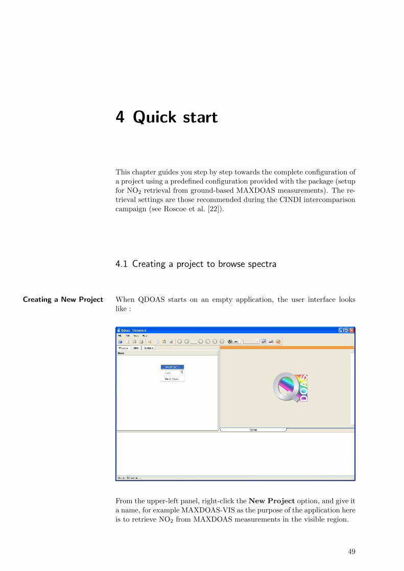
4 Quick start
This chapter guides you step by step towards the complete configuration ofa project using a predefined configuration provided with the package (setupfor NO2 retrieval from ground-based MAXDOAS measurements). The re-trieval settings are those recommended during the CINDI intercomparisoncampaign (see Roscoe et al. [22]).
4.1 Creating a project to browse spectra
Creating a New Project When QDOAS starts on an empty application, the user interface lookslike :
From the upper-left panel, right-click the New Project option, and give ita name, for example MAXDOAS-VIS as the purpose of the application hereis to retrieve NO2 from MAXDOAS measurements in the visible region.
49
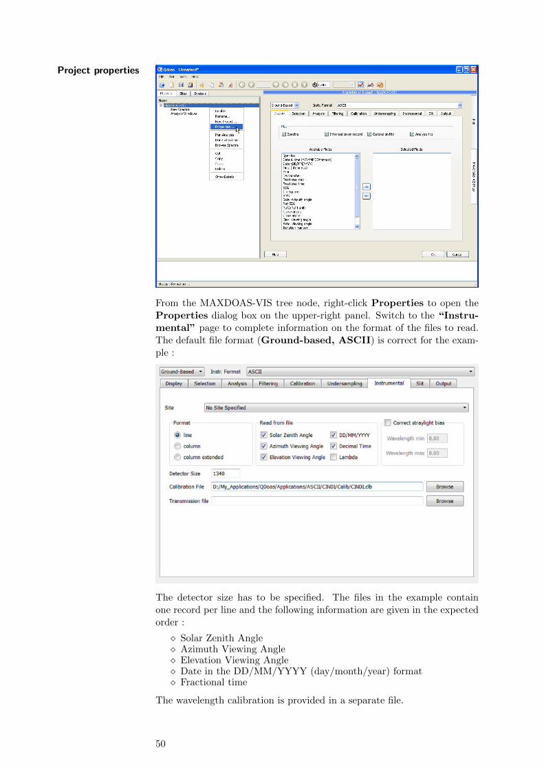
Project properties
From the MAXDOAS-VIS tree node, right-click Properties to open theProperties dialog box on the upper-right panel. Switch to the “Instru-mental” page to complete information on the format of the files to read.The default file format (Ground-based, ASCII) is correct for the exam-ple :
The detector size has to be specified. The files in the example containone record per line and the following information are given in the expectedorder :
� Solar Zenith Angle� Azimuth Viewing Angle� Elevation Viewing Angle� Date in the DD/MM/YYYY (day/month/year) format� Fractional time
The wavelength calibration is provided in a separate file.
50
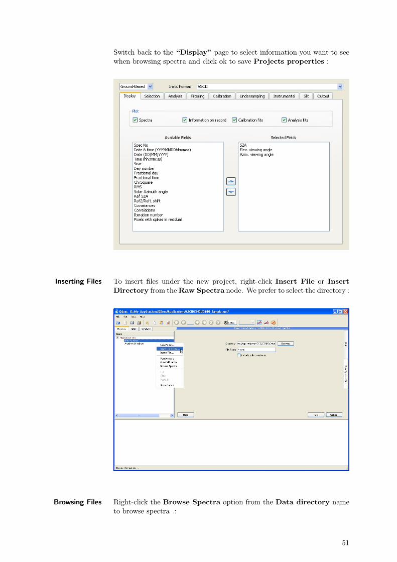
Switch back to the “Display” page to select information you want to seewhen browsing spectra and click ok to save Projects properties :
Inserting Files To insert files under the new project, right-click Insert File or InsertDirectory from the Raw Spectra node. We prefer to select the directory :
Browsing Files Right-click the Browse Spectra option from the Data directory nameto browse spectra :
51
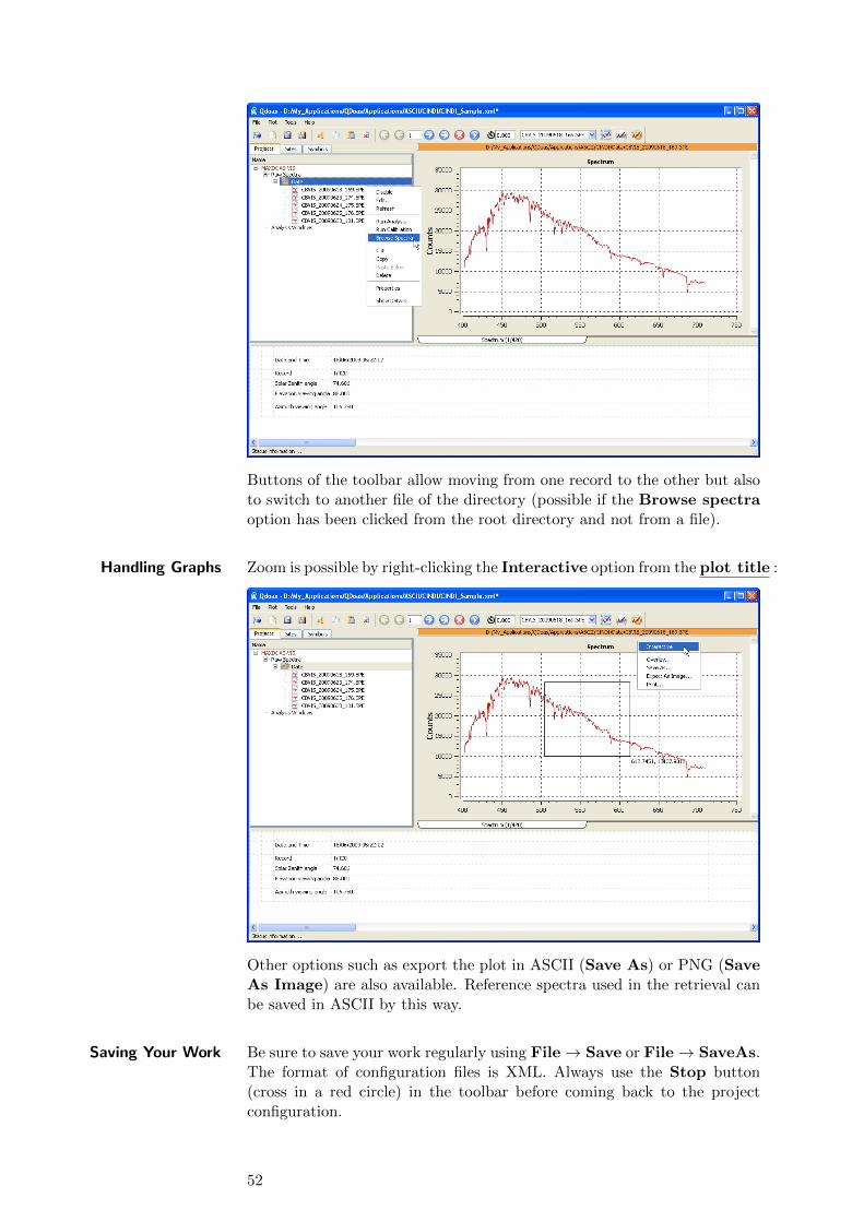
Buttons of the toolbar allow moving from one record to the other but alsoto switch to another file of the directory (possible if the Browse spectraoption has been clicked from the root directory and not from a file).
Handling Graphs Zoom is possible by right-clicking the Interactive option from the plot title :
Other options such as export the plot in ASCII (Save As) or PNG (SaveAs Image) are also available. Reference spectra used in the retrieval canbe saved in ASCII by this way.
Saving Your Work Be sure to save your work regularly using File→ Save or File→ SaveAs.The format of configuration files is XML. Always use the Stop button(cross in a red circle) in the toolbar before coming back to the projectconfiguration.
52
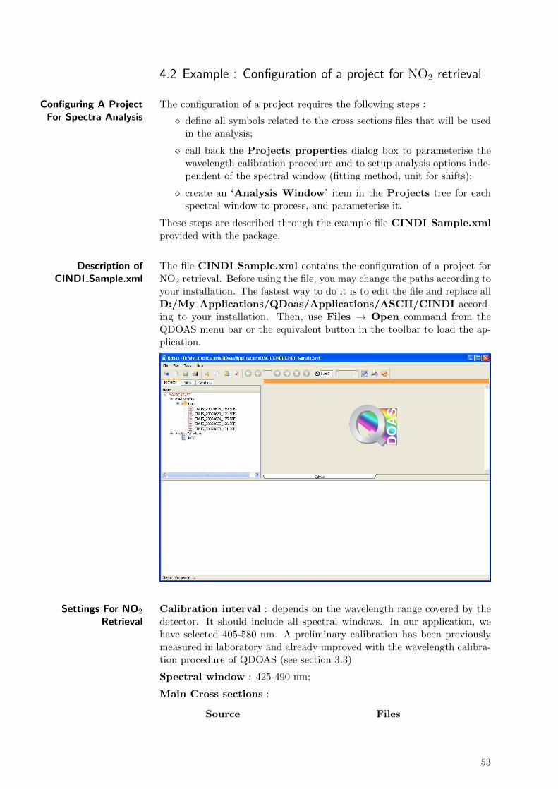
4.2 Example : Configuration of a project for NO2 retrieval
Configuring A ProjectFor Spectra Analysis
The configuration of a project requires the following steps :
� define all symbols related to the cross sections files that will be usedin the analysis;
� call back the Projects properties dialog box to parameterise thewavelength calibration procedure and to setup analysis options inde-pendent of the spectral window (fitting method, unit for shifts);
� create an ‘Analysis Window’ item in the Projects tree for eachspectral window to process, and parameterise it.
These steps are described through the example file CINDI Sample.xmlprovided with the package.
Description ofCINDI Sample.xml
The file CINDI Sample.xml contains the configuration of a project forNO2 retrieval. Before using the file, you may change the paths according toyour installation. The fastest way to do it is to edit the file and replace allD:/My Applications/QDoas/Applications/ASCII/CINDI accord-ing to your installation. Then, use Files → Open command from theQDOAS menu bar or the equivalent button in the toolbar to load the ap-plication.
Settings For NO2
RetrievalCalibration interval : depends on the wavelength range covered by thedetector. It should include all spectral windows. In our application, wehave selected 405-580 nm. A preliminary calibration has been previouslymeasured in laboratory and already improved with the wavelength calibra-tion procedure of QDOAS (see section 3.3)
Spectral window : 425-490 nm;
Main Cross sections :
Source Files
53

O3 Bogumil et al. [5], 223 K o3 223K Bogumil.xsNO2 Vandaele et al. [27], 298 K et 220 K no2 298K vanDaele.xs
no2a 220K vanDaele.xsO4 Hermans et al. o4 Hermans web.xsH2O From HITRAN data base h2o hitran.xsRing Ratio of the rotational raman spec-
trum by the solar one, both con-volved at the resolution of the in-strument with the Convolve Ringoption.
Ring NDSC2003.xs
The cross sections are those recommended during the CINDI intercompar-ison campaign (see Roscoe et al. [22]).
Defining Symbols The first thing to do is to define the cross sections symbols according tothe files names (see table above) : O3, NO2, NO2a, O4, H2O, Ring (thecase is not important). A description can be added. QDOAS needs thesesymbols for internal use.
Projects Properties
54
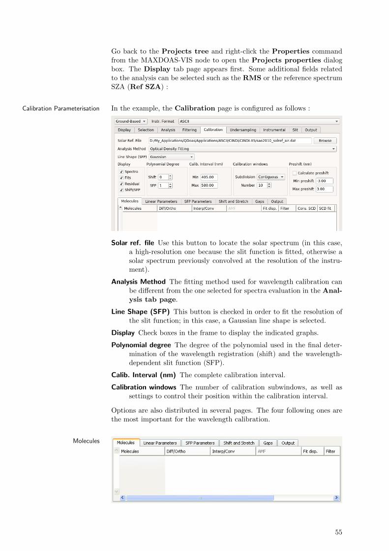
Go back to the Projects tree and right-click the Properties commandfrom the MAXDOAS-VIS node to open the Projects properties dialogbox. The Display tab page appears first. Some additional fields relatedto the analysis can be selected such as the RMS or the reference spectrumSZA (Ref SZA) :
Calibration Parameterisation In the example, the Calibration page is configured as follows :
Solar ref. file Use this button to locate the solar spectrum (in this case,a high-resolution one because the slit function is fitted, otherwise asolar spectrum previously convolved at the resolution of the instru-ment).
Analysis Method The fitting method used for wavelength calibration canbe different from the one selected for spectra evaluation in the Anal-ysis tab page.
Line Shape (SFP) This button is checked in order to fit the resolution ofthe slit function; in this case, a Gaussian line shape is selected.
Display Check boxes in the frame to display the indicated graphs.
Polynomial degree The degree of the polynomial used in the final deter-mination of the wavelength registration (shift) and the wavelength-dependent slit function (SFP).
Calib. Interval (nm) The complete calibration interval.
Calibration windows The number of calibration subwindows, as well assettings to control their position within the calibration interval.
Options are also distributed in several pages. The four following ones arethe most important for the wavelength calibration.
Molecules
55
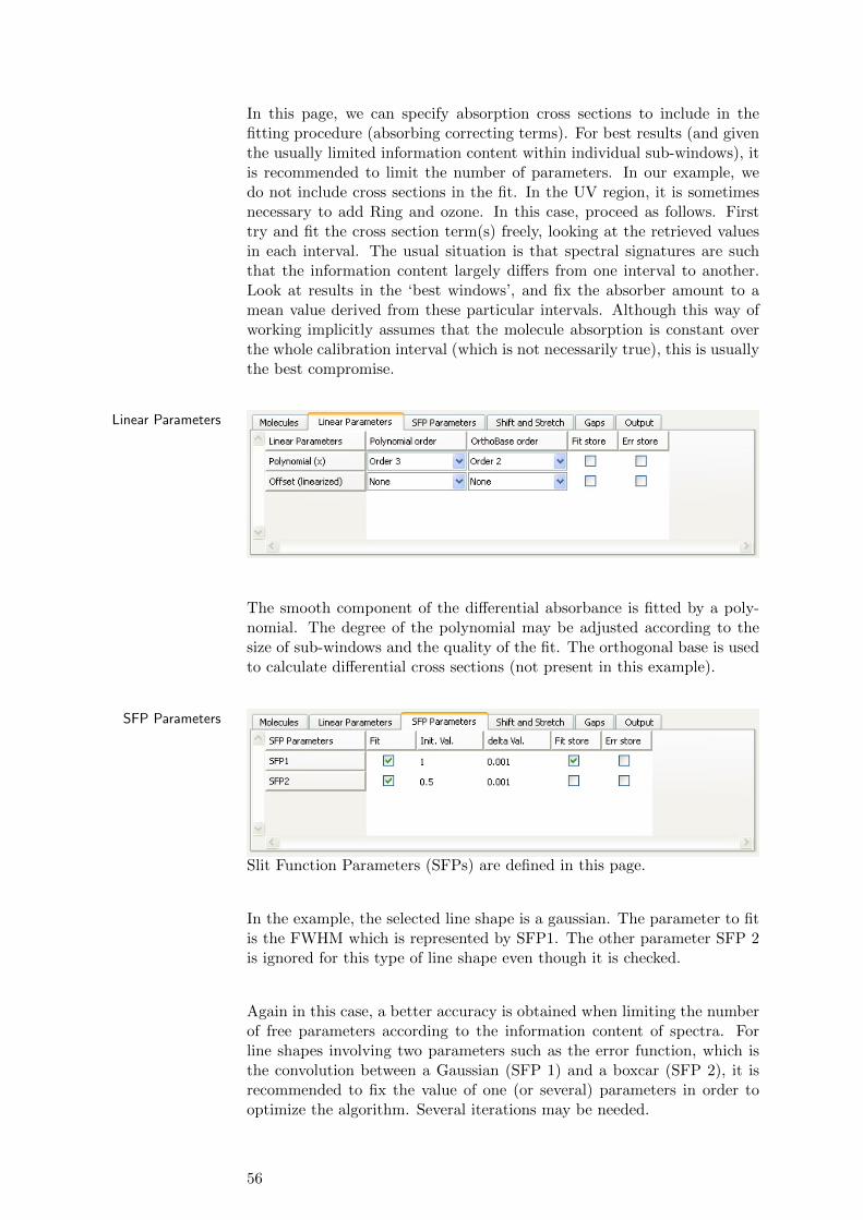
In this page, we can specify absorption cross sections to include in thefitting procedure (absorbing correcting terms). For best results (and giventhe usually limited information content within individual sub-windows), itis recommended to limit the number of parameters. In our example, wedo not include cross sections in the fit. In the UV region, it is sometimesnecessary to add Ring and ozone. In this case, proceed as follows. Firsttry and fit the cross section term(s) freely, looking at the retrieved valuesin each interval. The usual situation is that spectral signatures are suchthat the information content largely differs from one interval to another.Look at results in the ‘best windows’, and fix the absorber amount to amean value derived from these particular intervals. Although this way ofworking implicitly assumes that the molecule absorption is constant overthe whole calibration interval (which is not necessarily true), this is usuallythe best compromise.
Linear Parameters
The smooth component of the differential absorbance is fitted by a poly-nomial. The degree of the polynomial may be adjusted according to thesize of sub-windows and the quality of the fit. The orthogonal base is usedto calculate differential cross sections (not present in this example).
SFP Parameters
Slit Function Parameters (SFPs) are defined in this page.
In the example, the selected line shape is a gaussian. The parameter to fitis the FWHM which is represented by SFP1. The other parameter SFP 2is ignored for this type of line shape even though it is checked.
Again in this case, a better accuracy is obtained when limiting the numberof free parameters according to the information content of spectra. Forline shapes involving two parameters such as the error function, which isthe convolution between a Gaussian (SFP 1) and a boxcar (SFP 2), it isrecommended to fix the value of one (or several) parameters in order tooptimize the algorithm. Several iterations may be needed.
56
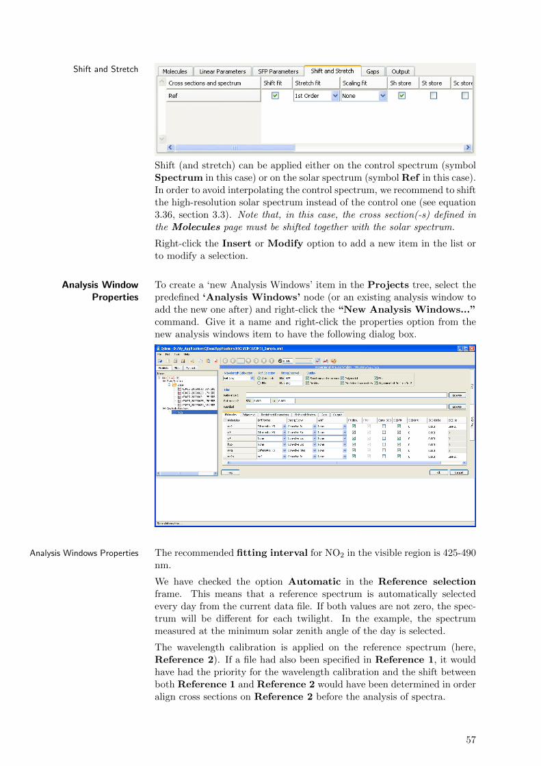
Shift and Stretch
Shift (and stretch) can be applied either on the control spectrum (symbolSpectrum in this case) or on the solar spectrum (symbol Ref in this case).In order to avoid interpolating the control spectrum, we recommend to shiftthe high-resolution solar spectrum instead of the control one (see equation3.36, section 3.3). Note that, in this case, the cross section(-s) defined inthe Molecules page must be shifted together with the solar spectrum.
Right-click the Insert or Modify option to add a new item in the list orto modify a selection.
Analysis WindowProperties
To create a ‘new Analysis Windows’ item in the Projects tree, select thepredefined ‘Analysis Windows’ node (or an existing analysis window toadd the new one after) and right-click the “New Analysis Windows...”command. Give it a name and right-click the properties option from thenew analysis windows item to have the following dialog box.
Analysis Windows Properties The recommended fitting interval for NO2 in the visible region is 425-490nm.
We have checked the option Automatic in the Reference selectionframe. This means that a reference spectrum is automatically selectedevery day from the current data file. If both values are not zero, the spec-trum will be different for each twilight. In the example, the spectrummeasured at the minimum solar zenith angle of the day is selected.
The wavelength calibration is applied on the reference spectrum (here,Reference 2). If a file had also been specified in Reference 1, it wouldhave had the priority for the wavelength calibration and the shift betweenboth Reference 1 and Reference 2 would have been determined in orderalign cross sections on Reference 2 before the analysis of spectra.
57
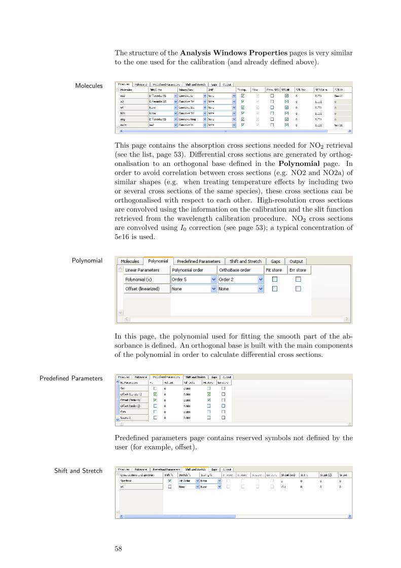
The structure of the Analysis Windows Properties pages is very similarto the one used for the calibration (and already defined above).
Molecules
This page contains the absorption cross sections needed for NO2 retrieval(see the list, page 53). Differential cross sections are generated by orthog-onalisation to an orthogonal base defined in the Polynomial page. Inorder to avoid correlation between cross sections (e.g. NO2 and NO2a) ofsimilar shapes (e.g. when treating temperature effects by including twoor several cross sections of the same species), these cross sections can beorthogonalised with respect to each other. High-resolution cross sectionsare convolved using the information on the calibration and the slit functionretrieved from the wavelength calibration procedure. NO2 cross sectionsare convolved using I0 correction (see page 53); a typical concentration of5e16 is used.
Polynomial
In this page, the polynomial used for fitting the smooth part of the ab-sorbance is defined. An orthogonal base is built with the main componentsof the polynomial in order to calculate differential cross sections.
Predefined Parameters
Predefined parameters page contains reserved symbols not defined by theuser (for example, offset).
Shift and Stretch
58
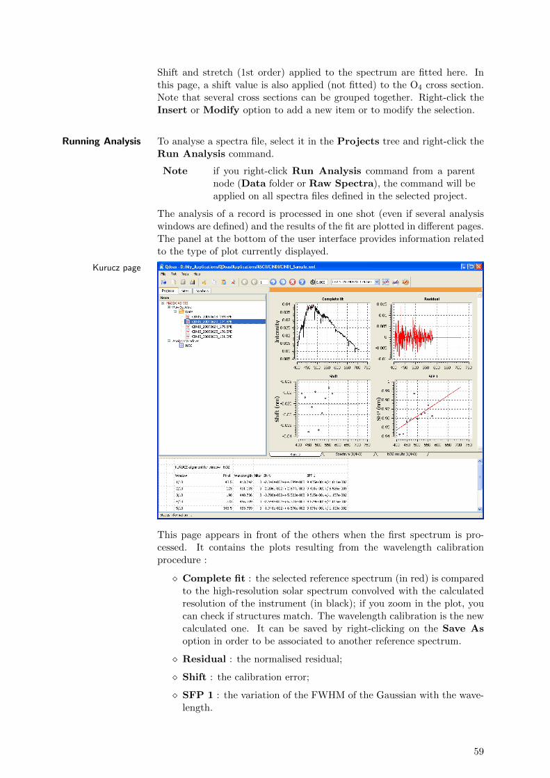
Shift and stretch (1st order) applied to the spectrum are fitted here. Inthis page, a shift value is also applied (not fitted) to the O4 cross section.Note that several cross sections can be grouped together. Right-click theInsert or Modify option to add a new item or to modify the selection.
Running Analysis To analyse a spectra file, select it in the Projects tree and right-click theRun Analysis command.
Note if you right-click Run Analysis command from a parentnode (Data folder or Raw Spectra), the command will beapplied on all spectra files defined in the selected project.
The analysis of a record is processed in one shot (even if several analysiswindows are defined) and the results of the fit are plotted in different pages.The panel at the bottom of the user interface provides information relatedto the type of plot currently displayed.
Kurucz page
This page appears in front of the others when the first spectrum is pro-cessed. It contains the plots resulting from the wavelength calibrationprocedure :
� Complete fit : the selected reference spectrum (in red) is comparedto the high-resolution solar spectrum convolved with the calculatedresolution of the instrument (in black); if you zoom in the plot, youcan check if structures match. The wavelength calibration is the newcalculated one. It can be saved by right-clicking on the Save Asoption in order to be associated to another reference spectrum.
� Residual : the normalised residual;
� Shift : the calibration error;
� SFP 1 : the variation of the FWHM of the Gaussian with the wave-length.
59
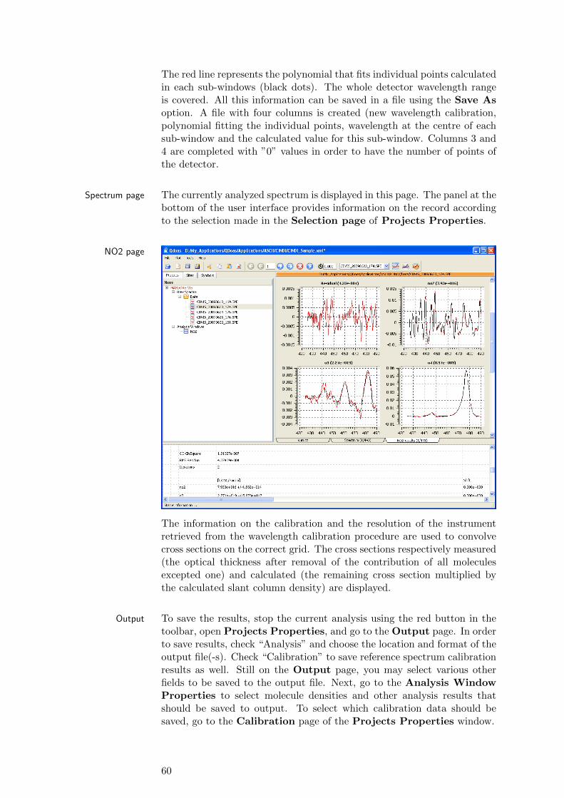
The red line represents the polynomial that fits individual points calculatedin each sub-windows (black dots). The whole detector wavelength rangeis covered. All this information can be saved in a file using the Save Asoption. A file with four columns is created (new wavelength calibration,polynomial fitting the individual points, wavelength at the centre of eachsub-window and the calculated value for this sub-window. Columns 3 and4 are completed with ”0” values in order to have the number of points ofthe detector.
Spectrum page The currently analyzed spectrum is displayed in this page. The panel at thebottom of the user interface provides information on the record accordingto the selection made in the Selection page of Projects Properties.
NO2 page
The information on the calibration and the resolution of the instrumentretrieved from the wavelength calibration procedure are used to convolvecross sections on the correct grid. The cross sections respectively measured(the optical thickness after removal of the contribution of all moleculesexcepted one) and calculated (the remaining cross section multiplied bythe calculated slant column density) are displayed.
Output To save the results, stop the current analysis using the red button in thetoolbar, open Projects Properties, and go to the Output page. In orderto save results, check “Analysis” and choose the location and format of theoutput file(-s). Check “Calibration” to save reference spectrum calibrationresults as well. Still on the Output page, you may select various otherfields to be saved to the output file. Next, go to the Analysis WindowProperties to select molecule densities and other analysis results thatshould be saved to output. To select which calibration data should besaved, go to the Calibration page of the Projects Properties window.
60
5 Projects and Analysis WindowsProperties
This chapter covers:
1. the configuration of projects;2. the parameterisation of the analysis;3. the parameterisation of the wavelength calibration.
5.1 Projects properties
The Projects properties dialog box resumes the general options to con-figure the application. These options are divided into the following cate-gories:
Display selection of information to display with spectra;
Selection selection of spectra to browse or to analyse;
Analysis options specific to the analysis (analysis method,interpolation, convergence criterion, . . . );
Filtering selection of a filtering method to apply on spec-tra and absorption cross sections;
Calibration configuration of the wavelength calibrationprocedure;
Undersampling selection of a method to calculate undersam-pling cross sections and to include them in thefit;
Instrumental options specific to the selected input file format;
Slit definition of a slit function or a method to con-volve cross sections before the analysis using theinformation generated by the wavelength cali-bration procedure;
Output selection of the information on the spectra thatshould be saved in the output file after theanalysis.
The creation of a new project always starts with the definition of the mea-surement type (satellite, ground-based or airborne) and the selection of the
61
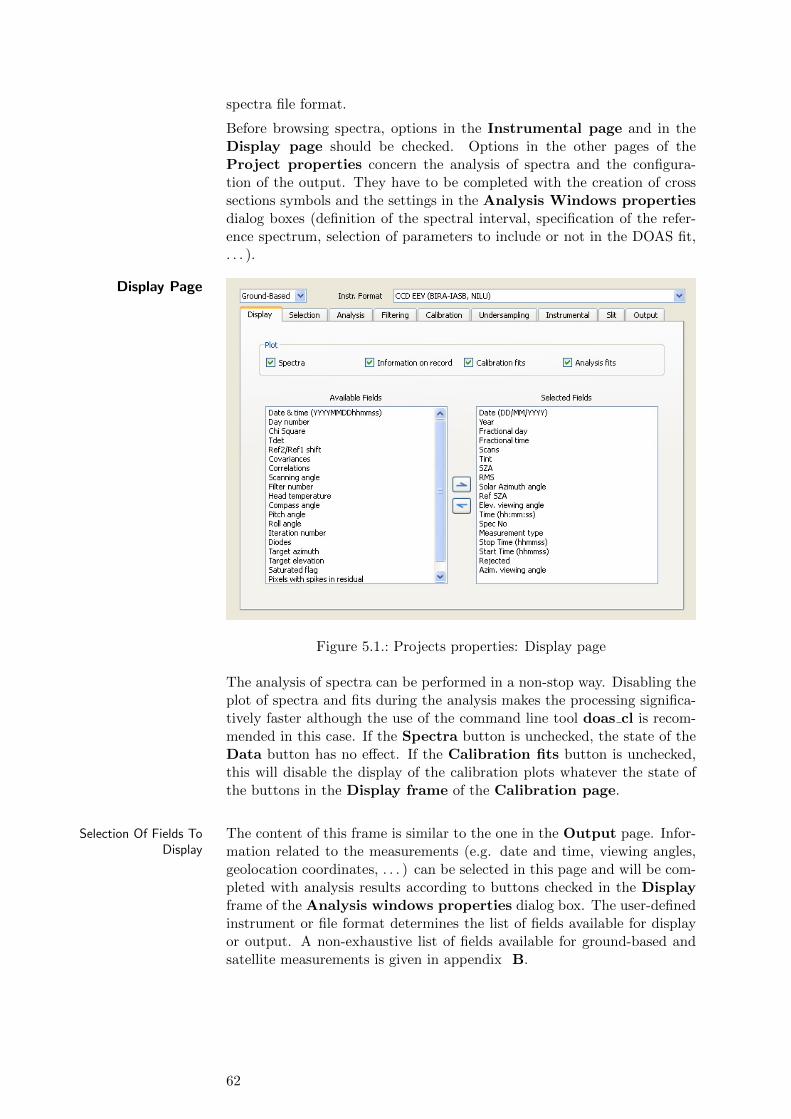
spectra file format.
Before browsing spectra, options in the Instrumental page and in theDisplay page should be checked. Options in the other pages of theProject properties concern the analysis of spectra and the configura-tion of the output. They have to be completed with the creation of crosssections symbols and the settings in the Analysis Windows propertiesdialog boxes (definition of the spectral interval, specification of the refer-ence spectrum, selection of parameters to include or not in the DOAS fit,. . . ).
Display Page
Figure 5.1.: Projects properties: Display page
The analysis of spectra can be performed in a non-stop way. Disabling theplot of spectra and fits during the analysis makes the processing significa-tively faster although the use of the command line tool doas cl is recom-mended in this case. If the Spectra button is unchecked, the state of theData button has no effect. If the Calibration fits button is unchecked,this will disable the display of the calibration plots whatever the state ofthe buttons in the Display frame of the Calibration page.
Selection Of Fields ToDisplay
The content of this frame is similar to the one in the Output page. Infor-mation related to the measurements (e.g. date and time, viewing angles,geolocation coordinates, . . . ) can be selected in this page and will be com-pleted with analysis results according to buttons checked in the Displayframe of the Analysis windows properties dialog box. The user-definedinstrument or file format determines the list of fields available for displayor output. A non-exhaustive list of fields available for ground-based andsatellite measurements is given in appendix B.
62
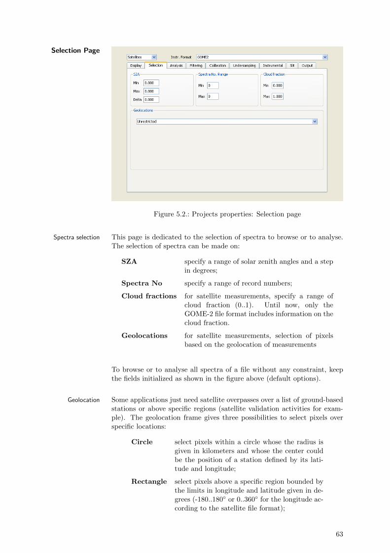
Selection Page
Figure 5.2.: Projects properties: Selection page
Spectra selection This page is dedicated to the selection of spectra to browse or to analyse.The selection of spectra can be made on:
SZA specify a range of solar zenith angles and a stepin degrees;
Spectra No specify a range of record numbers;
Cloud fractions for satellite measurements, specify a range ofcloud fraction (0..1). Until now, only theGOME-2 file format includes information on thecloud fraction.
Geolocations for satellite measurements, selection of pixelsbased on the geolocation of measurements
To browse or to analyse all spectra of a file without any constraint, keepthe fields initialized as shown in the figure above (default options).
Geolocation Some applications just need satellite overpasses over a list of ground-basedstations or above specific regions (satellite validation activities for exam-ple). The geolocation frame gives three possibilities to select pixels overspecific locations:
Circle select pixels within a circle whose the radius isgiven in kilometers and whose the center couldbe the position of a station defined by its lati-tude and longitude;
Rectangle select pixels above a specific region bounded bythe limits in longitude and latitude given in de-grees (-180..180◦ or 0..360◦ for the longitude ac-cording to the satellite file format);
63
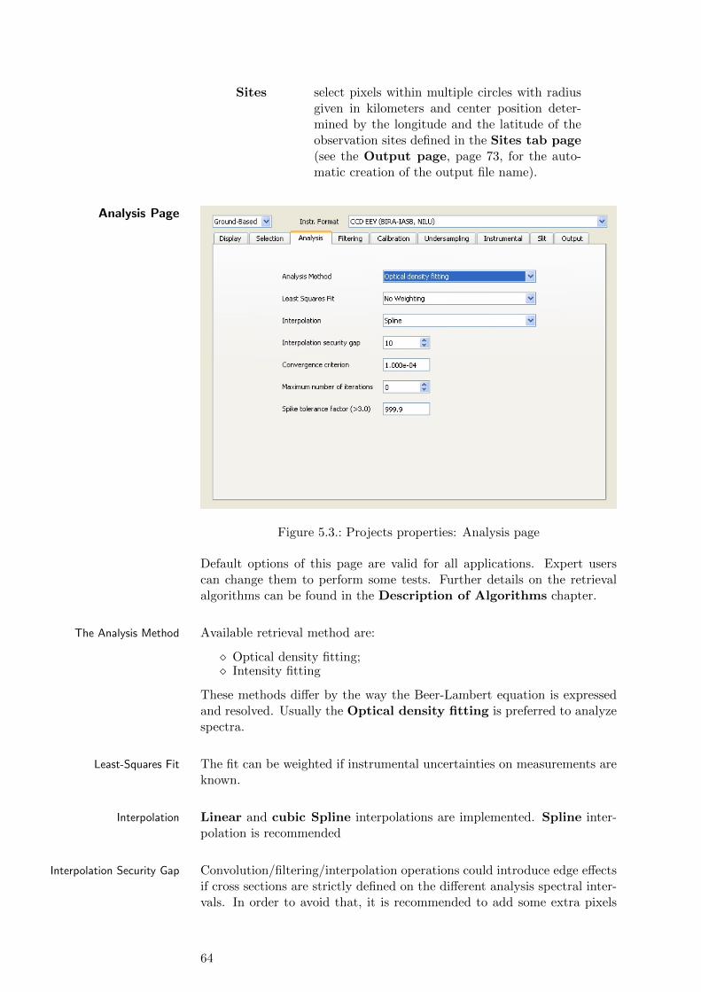
Sites select pixels within multiple circles with radiusgiven in kilometers and center position deter-mined by the longitude and the latitude of theobservation sites defined in the Sites tab page(see the Output page, page 73, for the auto-matic creation of the output file name).
Analysis Page
Figure 5.3.: Projects properties: Analysis page
Default options of this page are valid for all applications. Expert userscan change them to perform some tests. Further details on the retrievalalgorithms can be found in the Description of Algorithms chapter.
The Analysis Method Available retrieval method are:
� Optical density fitting;� Intensity fitting
These methods differ by the way the Beer-Lambert equation is expressedand resolved. Usually the Optical density fitting is preferred to analyzespectra.
Least-Squares Fit The fit can be weighted if instrumental uncertainties on measurements areknown.
Interpolation Linear and cubic Spline interpolations are implemented. Spline inter-polation is recommended
Interpolation Security Gap Convolution/filtering/interpolation operations could introduce edge effectsif cross sections are strictly defined on the different analysis spectral inter-vals. In order to avoid that, it is recommended to add some extra pixels
64

on both sides of the final grid. The security gap determines this number ofpixels. If the selected filter requires a larger number of additional pixels,the gap is recalculated by QDOAS.
Convergence Criterion As explained in the description of the Marquardt-Levenberg Algorithm insection 3.2, the NLLS algorithm uses the convergence criterion to determinewhen it has arrived at a solution.
Usually a value of 1e-3 or 1e-4 is selected for the convergence criterion. Forhigher values of ε, the algorithm will use less iterations, but the accuracyof the results could be affected.
Maximum Number ofIterations
The number of iterations needed to analyze a spectrum is determined bythe convergence speed of the Marquardt-Levenberg algorithm for this spec-trum. For some tests, it is sometimes useful to limit it. A value of “0”doesn’t limit the number of iterations.
Spike Tolerance Factor Spikes removal is a good alternative to the introduction of gaps (see theGaps section of Analysis windows properties, page 86 to automati-cally remove bad data points from the fit, such as satellite measurementsaffected by the South Atlantic Anomaly or pixels of the detector damagedby electronic radiation. To do this, QDOAS calculates the Root MeanSquare (RMS) residual after the fit. If a pixel i is found where the absolutevalue of the residual, Ri, exceeds the RMS by more than the spike tolerancefactor x,
Ri > x · RMS , (5.1)
QDOAS will remove this pixel from the analysis and calculate a new fit.This procedure is applied iteratively until no residuals exceed the RMS bymore than the given tolerance factor. The analysis results contain a list ofall pixels that were removed.
This feature should be used with caution, as choosing a too low tolerancefactor might exclude valid data points from the fit. Assuming the residualsare normally distributed with mean 0, the RMS can be used as an estimateof the standard deviation σ. As a rule of thumb, the tolerance factorx should be high enough, so the probability that a normally distributedrandom variable lies outside a range of x · σ around the mean, multipliedby the number of pixels in the analysis window, is small.
65
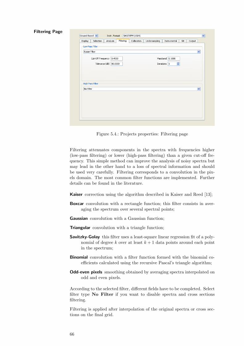
Filtering Page
Figure 5.4.: Projects properties: Filtering page
Filtering attenuates components in the spectra with frequencies higher(low-pass filtering) or lower (high-pass filtering) than a given cut-off fre-quency. This simple method can improve the analysis of noisy spectra butmay lead in the other hand to a loss of spectral information and shouldbe used very carefully. Filtering corresponds to a convolution in the pix-els domain. The most common filter functions are implemented. Furtherdetails can be found in the literature.
Kaiser correction using the algorithm described in Kaiser and Reed [13];
Boxcar convolution with a rectangle function; this filter consists in aver-aging the spectrum over several spectral points;
Gaussian convolution with a Gaussian function;
Triangular convolution with a triangle function;
Savitzky-Golay this filter uses a least-square linear regression fit of a poly-nomial of degree k over at least k + 1 data points around each pointin the spectrum;
Binomial convolution with a filter function formed with the binomial co-efficients calculated using the recursive Pascal’s triangle algorithm;
Odd-even pixels smoothing obtained by averaging spectra interpolated onodd and even pixels.
According to the selected filter, different fields have to be completed. Selectfilter type No Filter if you want to disable spectra and cross sectionsfiltering.
Filtering is applied after interpolation of the original spectra or cross sec-tions on the final grid.
66

Low-Pass Filtering Low-pass filtering is applied to the spectra and to the cross sections. Nev-ertheless, the filtering of cross sections could be disabled individually inthe Analysis windows properties dialog box.
High-Pass Filtering Cross sections are filtered by subtracting (optical density fitting) or dividing(intensity fitting) a fitted polynomial or a smooth spectrum calculated byfiltering the original cross sections a high number of times. This can be analternative to the Gram-Schmidt algorithm to calculate differential crosssections.
For the moment, high-pass filtering is supported only in optical densityfitting mode. It can be applied during the phase of calibration and/orduring the analysis of spectra.
Calibration Page The configurtion of the wavelength calibration procedure is explained indetail in section 5.4.
Undersampling Page
Figure 5.5.: Projects properties: Undersampling page
The undersampling is a well-known problem of GOME onboard the satelliteERS-2. It arises from the poor sampling ratio of the GOME instrument (2to 3 pixels/FWHM of the resolution of the spectrometer) which results ina lost of spectral information when interpolating earthshine spectra duringthe DOAS fitting process. The problem can be corrected using ad-hoccross sections obtained by simulating the effect from a high-resolution solarreference. Undersampling cross sections can be pre-calculated using theThe undersampling tool (usamp) or they can be calculated in realtime, just after the wavelength calibration procedure using the correctedgrid and the determined slit function.
To apply undersampling correction, the fit button of Usamp 1 and/orUsamp 2 items in the Predefined parameters page of Analysis win-dows properties (cfr page 84) has to be checked in addition of the se-lection of options of this page. By default, no undersampling correction is
67
applied.
Method Different methods for the calculation of the undersampling correction areavailable.
From file Undersampling cross sections are provided infiles like usual cross sections. These files mightbe created using the The undersampling tool(usamp). The files have to be provided in theAnalysis windows properties (Molecules orPredefined paremeters page according to theselected analysis method).
Fixed phase QDOAS uses the information derived from thecalibration procedure to create the undersam-pling cross sections, with a fixed value ofthe shift. The selection of this method isrecommended.
Automatic phase The undersampling cross sections are calculatedat each iteration of the analysis procedure, usingthe fitted value for the shift between the refer-ence and the measured spectra. This method israther time consuming and only applicable fortesting purposes.
Solar ref. file In Fixed phase and Automatic phase, undersampling cross sections arecalculated from a high resolution solar spectrum convolved on an oversam-pled and an undersampled grid with the instrument slit function (accordingto calibration options, the slit function characterized by the calibra-tion procedure or a slit function provided by the user in the slit page ofProjects properties).
Shift The Shift field operates only in Fixed phase method.
68
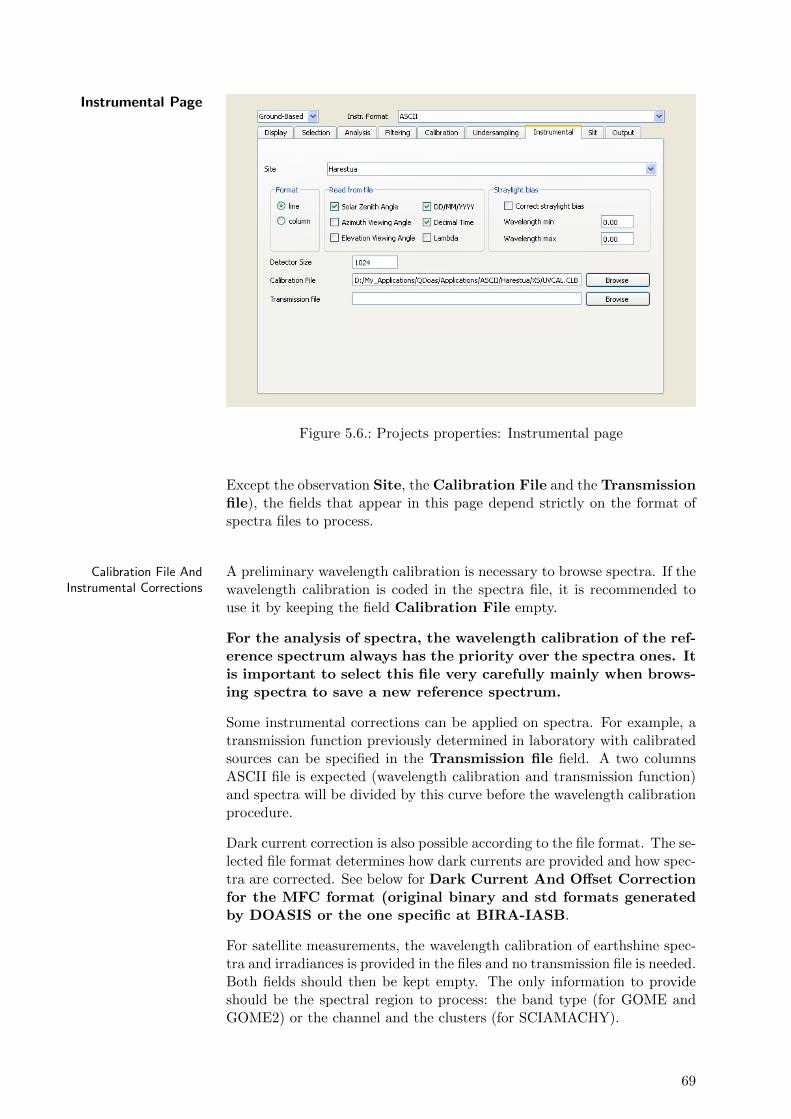
Instrumental Page
Figure 5.6.: Projects properties: Instrumental page
Except the observation Site, the Calibration File and the Transmissionfile), the fields that appear in this page depend strictly on the format ofspectra files to process.
Calibration File AndInstrumental Corrections
A preliminary wavelength calibration is necessary to browse spectra. If thewavelength calibration is coded in the spectra file, it is recommended touse it by keeping the field Calibration File empty.
For the analysis of spectra, the wavelength calibration of the ref-erence spectrum always has the priority over the spectra ones. Itis important to select this file very carefully mainly when brows-ing spectra to save a new reference spectrum.
Some instrumental corrections can be applied on spectra. For example, atransmission function previously determined in laboratory with calibratedsources can be specified in the Transmission file field. A two columnsASCII file is expected (wavelength calibration and transmission function)and spectra will be divided by this curve before the wavelength calibrationprocedure.
Dark current correction is also possible according to the file format. The se-lected file format determines how dark currents are provided and how spec-tra are corrected. See below for Dark Current And Offset Correctionfor the MFC format (original binary and std formats generatedby DOASIS or the one specific at BIRA-IASB.
For satellite measurements, the wavelength calibration of earthshine spec-tra and irradiances is provided in the files and no transmission file is needed.Both fields should then be kept empty. The only information to provideshould be the spectral region to process: the band type (for GOME andGOME2) or the channel and the clusters (for SCIAMACHY).
69

Dark Current And OffsetCorrection For The MFC
Format
According to the file format, measured dark current are available and sub-tracted from spectra just before the analysis. Since version 2.111, QDOASsupports both MFC binary and STD ASCII formats generated by the well-known DOASIS program created by the atmospheric research group at IUPHeidelberg, Germany and widely used in the DOAS community.
https://doasis.iup.uni-heidelberg.de/bugtracker/projects/doasis/
In addition, BIRA-IASB has developed its own binary MFC format inwhich all spectra including dark currents and offsets of a same day aresaved in a unique file. A MFC STD to MFC BIRA-IASB binary formatconverter exists (see the MFC Binary section, page 10).
For the BIRA-IASB binary format, dark currents and offsets present ina file are averaged before spectra correction. For the MFC binary andstd formats generated by DOASIS, dark current and offset are provided intwo separate files in the original format. Dark currents should be spectrameasured with a large integration time (typically 30 sec) and offsets shouldbe the average of a large number of spectra measured with a very smallintegration time (typically 1000 x 3 ms).
Application of the offset correction:
spe′ = spe− offset · (scansspe/scansoffset) , (5.2)
drk′ = drk− offset · (scansdrk/scansoffset) , (5.3)
where scansspe, scansdrk and scansoffset are respectively the number of scansfor the spectrum, the dark current and the offset.
Correction of spectra with the dark current (previously corrected by offset):
spe′ = spe− drk · (etspe · scansspe)/(etdrk · scansdrk) , (5.4)
where etspe and etdrk are respectively the exposure time of the spectrum andthe dark current and scansdrk is the number of scans of the dark current.
The Observation Site The information on the observation Site is used to (re)calculate solar zenithangle from geolocation coordinates given for this site in the Sites sheet.This can be useful for example if the solar zenith angles saved in the files arenot reliable enough. The abbreviation of the observation site is also used toautomatically generate output file names (see the Output Page, page 73).The longitude is particularly useful to select reference spectra of the dayusing the local time instead of Universal Time in case fractional days andtimes given in UT are distributed in two days (for example, measurementsin China).
Straylight bias Requested for some spectra files format, this option allows subtracting froma spectrum the signal averaged on the specified range of wavelengths. Thisis useful for example, to retrieve SO2 in the UV region where the signal isvery poor and where the straylight is problematic. Even if the straylightcan be attenuated by subtracting from the spectra, the average of the signalmeasured in the UV region (below 300 nm if possible), it is recommendedto characterize it in laboratory.
70
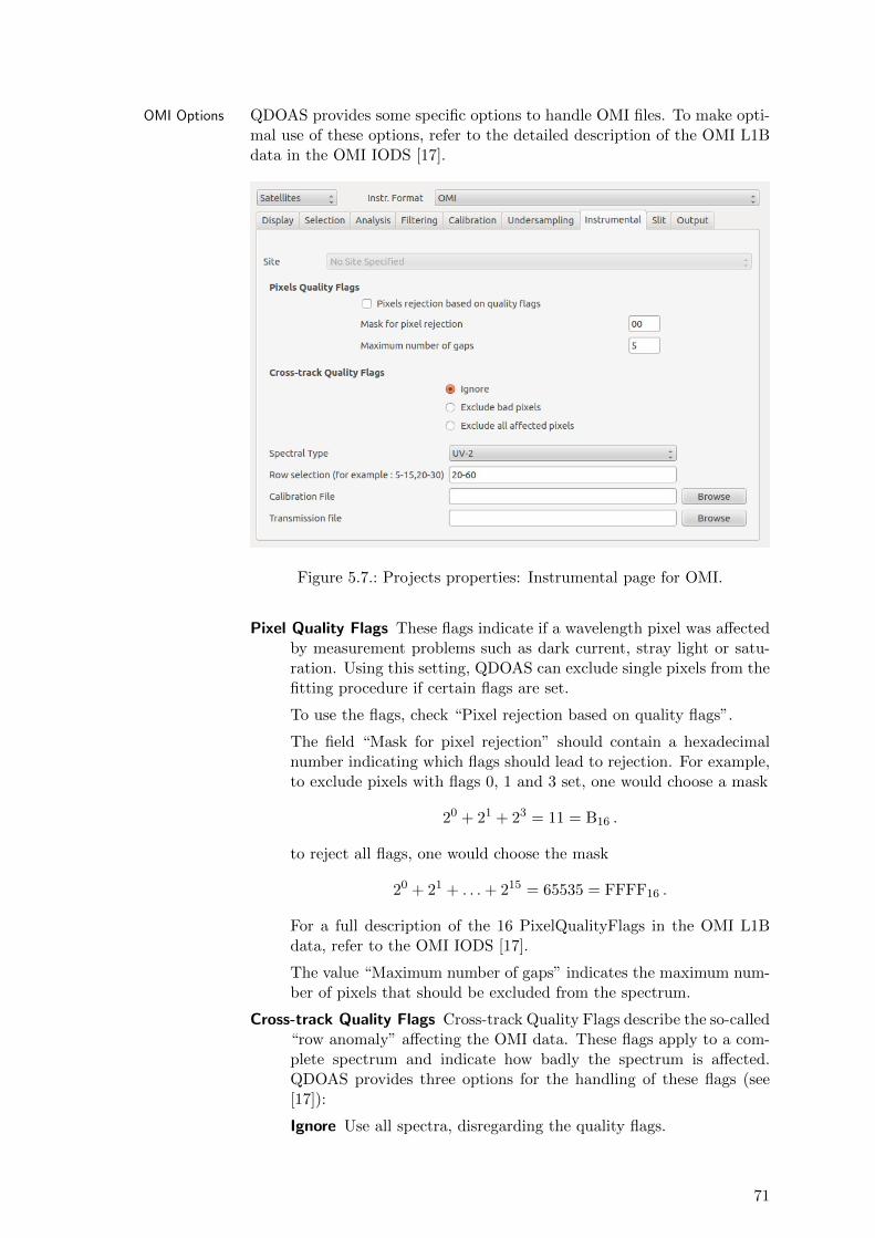
OMI Options QDOAS provides some specific options to handle OMI files. To make opti-mal use of these options, refer to the detailed description of the OMI L1Bdata in the OMI IODS [17].
Figure 5.7.: Projects properties: Instrumental page for OMI.
Pixel Quality Flags These flags indicate if a wavelength pixel was affectedby measurement problems such as dark current, stray light or satu-ration. Using this setting, QDOAS can exclude single pixels from thefitting procedure if certain flags are set.
To use the flags, check “Pixel rejection based on quality flags”.
The field “Mask for pixel rejection” should contain a hexadecimalnumber indicating which flags should lead to rejection. For example,to exclude pixels with flags 0, 1 and 3 set, one would choose a mask
20 + 21 + 23 = 11 = B16 .
to reject all flags, one would choose the mask
20 + 21 + . . .+ 215 = 65535 = FFFF16 .
For a full description of the 16 PixelQualityFlags in the OMI L1Bdata, refer to the OMI IODS [17].
The value “Maximum number of gaps” indicates the maximum num-ber of pixels that should be excluded from the spectrum.
Cross-track Quality Flags Cross-track Quality Flags describe the so-called“row anomaly” affecting the OMI data. These flags apply to a com-plete spectrum and indicate how badly the spectrum is affected.QDOAS provides three options for the handling of these flags (see[17]):
Ignore Use all spectra, disregarding the quality flags.
71

Exclude bad pixels Only exclude rows flagged as ’Affected, Not cor-rected, do not use’ in the L1B data.
Exclude all affected pixels Only use rows flagged as ’Not affected’.
Spectral Type OMI measurements contain data from three spectral bands:UV-1, UV-2 and VIS.
Row selection This option allows the user to select a subset of the 60detector rows for the analysis, by providing a list of ranges from 1 to60.
Slit Page
Figure 5.8.: Projects properties: Slit page
Input cross sections have to be degraded to the resolution of the instrumentbefore the analysis. This can be done using the convolution tool. How-ever the programme also authorizes the direct use of high-resolution crosssections which will be convolved in real time using information providedin this page if and only if the slit function is not characterized by thewavelength calibration procedure.
Slit Function Type Several analytic line shapes are proposed including line shapes supportedby the wavelength calibration procedure (gaussian, lorentzian, errorfunction, voigt and asymmetric line shapes). Different fields have to becompleted according to the selected slit function. ASCII file is requestedfor slit functions measured in laboratory (option File) or when the “Wave-length dependent” button is checked (analytical line shapes).
� Slit functions measured in laboratory: the first column should be thewavelength grid of the line shape; the maximum of the line shape isexpected around 0 nm; look-up tables can be specified for line shapesdefined at different wavelengths (in this case, the first line gives theindividual wavelengths).
� Wavelength dependent analytical slit functions: the input file shouldcontain the FWHM variation with the wavelenth calibration; at a
72
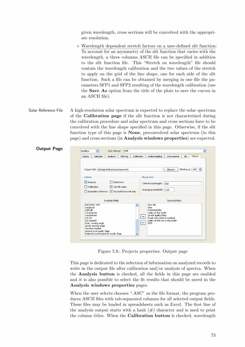
given wavelength, cross sections will be convolved with the appropri-ate resolution.
� Wavelength dependent stretch factors on a user-defined slit function:To account for an asymmetry of the slit function that varies with thewavelength, a three columns ASCII file can be specified in additionto the slit function file. This “Stretch on wavelength” file shouldcontain the wavelength calibration and the two values of the stretchto apply on the grid of the line shape, one for each side of the slitfunction. Such a file can be obtained by merging in one file the pa-rameters SFP1 and SFP2 resulting of the wavelength calibration (usethe Save As option from the title of the plots to save the curves inan ASCII file).
Solar Reference File A high-resolution solar spectrum is expected to replace the solar spectrumof the Calibration page if the slit function is not characterized duringthe calibration procedure and solar spectrum and cross sections have to beconvolved with the line shape specified in this page. Otherwise, if the slitfunction type of this page is None, preconvolved solar spectrum (in thispage) and cross sections (in Analysis windows properties) are expected.
Output Page
Figure 5.9.: Projects properties: Output page
This page is dedicated to the selection of information on analyzed records towrite in the output file after calibration and/or analysis of spectra. Whenthe Analysis button is checked, all the fields in this page are enabledand it is also possible to select the fit results that should be saved in theAnalysis windows properties pages.
When the user selects chooses “.ASC” as the file format, the program pro-duces ASCII files with tab-separated columns for all selected output fields.These files may be loaded in spreadsheets such as Excel. The first line ofthe analysis output starts with a hash (#) character and is used to printthe column titles. When the Calibration button is checked, wavelength
73

calibration results are saved before the analysis results. Lines with calibra-tion output start with a semicolon (;). If an ASCII output file alreadyexists at the specified location, QDOAS appends the new resultsto the existing file. In this case, column titles and calibration informa-tion are not repeated. Therefore, it is best to avoid writing to existingfiles, unless exactly the same analysis and output configuration is used toproduce the new data. To replace the content of an existing outputfile, the file must first be deleted manually.
With the file format “.nc”, QDOAS will produce netCDF output data.This is the recommended setting for users who wish to use a binary outputformat. In contrast to ASCII mode, results from different processing runscannot be appended to the same file in netCDF mode, unless the userchooses a different group name for both runs (the default group nameis “QDOAS Results”). When using QDOAS with a single output file,the program will check if the file already exists and report an error ifthe chosen output file cannot be used. However, when writing files in“automatic” mode (see Automatic Creation Of The Output File Name),QDOAS doesn’t check in advance which output file(-s) it will have to write,and it is left to the user to make sure that there are no existing files inthe output path which will prevent QDOAS from saving the results of aprocessing run.
When the user selects the file format “.he5”, QDOAS produces HDF-EOS51
output files. In HDF-EOS5 output mode, QDOAS saves data either as a“geolocation field” or as a “data field”, depending on the kind of informa-tion contained in the field. As for netCDF files, QDOAS will not writeoutput into an existing HDF-EOS5 file.
QDOAS always saves all the output from a single input file in one shot,either when it has processed the last spectrum of an input file, or when theanalysis is stopped using the stop button .
By default, QDOAS only saves records successfully analyzed. If the buttonSuccessful records only is kept unchecked, all records including refer-ence spectra and records for which the analysis fails (e.g. log error on thespectrum) are saved.
When processing was unsuccessful, QDOAS uses the fill value 9.969. . . e+36for floating point output data, an empty string for text output fields, andvalues -32767, 65535 or -2147483647 for integer output fields, depending onthe range of the output field. For HDF-EOS5 and netCDF output formats,the fill values are documented in the file metadata.
Automatic Creation Of TheOutput File Name
The path and the name of the output file can be specified in the OutputPath field. If “automatic” is used as a file name, QDOAS will generate thename of the output file automatically, using the user-defined output pathas a base.
For ground-based measurements, the Directories and Automatic refer-ence buttons have no effect. The original file name is always used (but thefile extension is changed in “.asc”) except if the Use file name button is
1HDF-EOS5 is a binary output format based on the HDF5 format see http://www.
hdfeos.org.
74
unchecked and an observation site has been specified in the Instrumentalpage. In this case, the output file name is built as follows:
<output path>/XXYYYYMM.ASC
Where:
output path is the user-defined path;
XX is the abbreviation of the observation site se-lected in the Instrumental tab page; if no ob-servation site is specified, the original file nameis used;
YYYY is the year of measurement;
MM is the month (zeros padded) of measurement;
ASC is the default file extension for ASCII files;
For satellite measurements, the Use file name button has no effect. Ifoverpasses calculation is requested (option Sites in the Geolocation frameof the Selection page), then the output file name is determined as above(<output path>/XXYYYYMM.ASC where XX is the abbreviation of thestation). Otherwise, for SCIAMACHY files, the output file name auto-matically created has the syntax SCIA YYYYMMDD NNNN.ASC whereYYYYMMDD is the date of measurement (year, month, day) and NNNNthe orbit number. For other satellite formats, the original file name isused (but with the file extension “.ASC”). Files are distributed in ayear/month/day folder structure if the Directories button is checked.
Fluxes The flux is the value of the signal averaged over pixels within a bandwitharound the specified wavelength. Divided by the exposure time, this canbe used to check a relative intensity. To calculate and save fluxes in theoutput file, specify the central wavelengths separated by the semicolon (;)character. For example, to get fluxes at 330 nm, 350 nm and 380 nm, enter:
330; 350; 380;
From version 2.107, the averaging bandwidth in nm is also requested (forexample a bandwidth of 1 nm means that pixels within the central wave-length +/- 0.5 nm will be averaged). But it is not possible to outputcolour indexes anymore. The colour index is the ratio between two fluxes;the calculation outside QDOAS is easy if both fluxes are output.
Selection Of Fields ToOutput
The content of this frame is similar to the one in the Display page. InQDOAS, the output is fully configurable. Information related to the mea-surements (e.g. date and time, viewing angles, geolocation coordinates, . . . )can be selected in this page. The selection of analysis results (e.g. slantcolumn densities, fitted non-linear parameters, . . . ) is made individuallyin the Analysis windows properties pages. The selected instrumentor file format determines the list of fields available for output. For ex-ample, information on cloud fraction and cloud top pressure is available
75
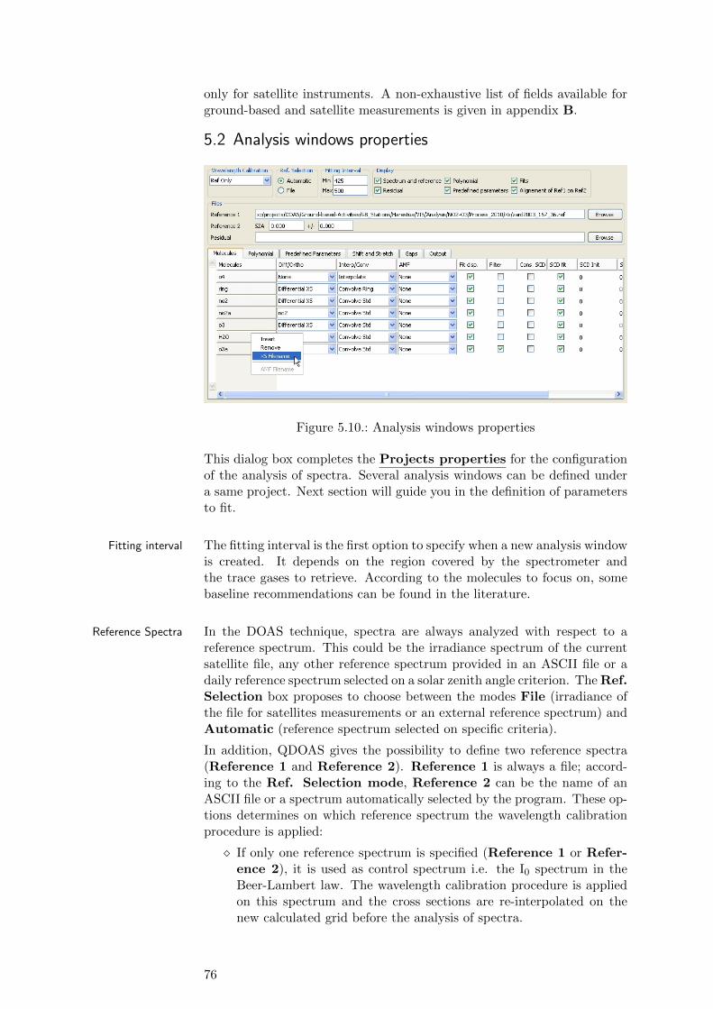
only for satellite instruments. A non-exhaustive list of fields available forground-based and satellite measurements is given in appendix B.
5.2 Analysis windows properties
Figure 5.10.: Analysis windows properties
This dialog box completes the Projects properties for the configurationof the analysis of spectra. Several analysis windows can be defined undera same project. Next section will guide you in the definition of parametersto fit.
Fitting interval The fitting interval is the first option to specify when a new analysis windowis created. It depends on the region covered by the spectrometer andthe trace gases to retrieve. According to the molecules to focus on, somebaseline recommendations can be found in the literature.
Reference Spectra In the DOAS technique, spectra are always analyzed with respect to areference spectrum. This could be the irradiance spectrum of the currentsatellite file, any other reference spectrum provided in an ASCII file or adaily reference spectrum selected on a solar zenith angle criterion. The Ref.Selection box proposes to choose between the modes File (irradiance ofthe file for satellites measurements or an external reference spectrum) andAutomatic (reference spectrum selected on specific criteria).
In addition, QDOAS gives the possibility to define two reference spectra(Reference 1 and Reference 2). Reference 1 is always a file; accord-ing to the Ref. Selection mode, Reference 2 can be the name of anASCII file or a spectrum automatically selected by the program. These op-tions determines on which reference spectrum the wavelength calibrationprocedure is applied:
� If only one reference spectrum is specified (Reference 1 or Refer-ence 2), it is used as control spectrum i.e. the I0 spectrum in theBeer-Lambert law. The wavelength calibration procedure is appliedon this spectrum and the cross sections are re-interpolated on thenew calculated grid before the analysis of spectra.
76
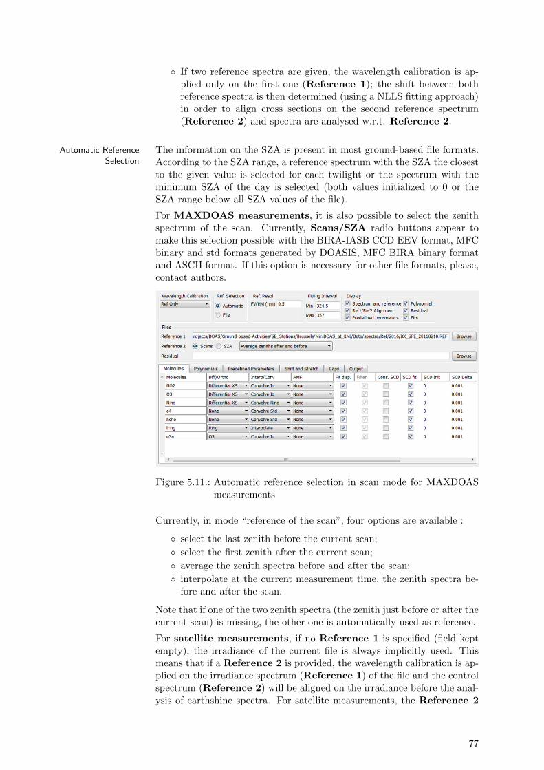
� If two reference spectra are given, the wavelength calibration is ap-plied only on the first one (Reference 1); the shift between bothreference spectra is then determined (using a NLLS fitting approach)in order to align cross sections on the second reference spectrum(Reference 2) and spectra are analysed w.r.t. Reference 2.
Automatic ReferenceSelection
The information on the SZA is present in most ground-based file formats.According to the SZA range, a reference spectrum with the SZA the closestto the given value is selected for each twilight or the spectrum with theminimum SZA of the day is selected (both values initialized to 0 or theSZA range below all SZA values of the file).
For MAXDOAS measurements, it is also possible to select the zenithspectrum of the scan. Currently, Scans/SZA radio buttons appear tomake this selection possible with the BIRA-IASB CCD EEV format, MFCbinary and std formats generated by DOASIS, MFC BIRA binary formatand ASCII format. If this option is necessary for other file formats, please,contact authors.
Figure 5.11.: Automatic reference selection in scan mode for MAXDOASmeasurements
Currently, in mode “reference of the scan”, four options are available :
� select the last zenith before the current scan;
� select the first zenith after the current scan;
� average the zenith spectra before and after the scan;
� interpolate at the current measurement time, the zenith spectra be-fore and after the scan.
Note that if one of the two zenith spectra (the zenith just before or after thecurrent scan) is missing, the other one is automatically used as reference.
For satellite measurements, if no Reference 1 is specified (field keptempty), the irradiance of the current file is always implicitly used. Thismeans that if a Reference 2 is provided, the wavelength calibration is ap-plied on the irradiance spectrum (Reference 1) of the file and the controlspectrum (Reference 2) will be aligned on the irradiance before the anal-ysis of earthshine spectra. For satellite measurements, the Reference 2
77
spectrum could be an average of spectra selected in a specific region givenby its minimum and maximum latitudes and longitudes. Other informa-tion such as the cloud fraction (GOME2) could also be used to refine thereference selection.
Wavelength Calibration The quality of the fit results largely relies on a very accurate determinationof the wavelength calibration of the reference spectrum. The wavelengthcalibration procedure developed in QDOAS allows correcting the prelimi-nary grid of the reference spectrum using a high-resolution solar atlas spec-trum degraded to the resolution of the instrument (see the Calibrationpage, page 67 of Projects properties). The information on the shiftand eventually the slit function retrieved from this procedure are used toconvolve/interpolate the cross sections before the analysis. The wavelengthcalibration is always applied in priority on the Reference 1 (the irradi-ance spectrum for satellite measurements). If two reference spectra areprovided, Reference 2 is aligned on Reference 1 using the same nonlinear least-square algorithm as the one used for the analysis of spectraw.r.t. the control spectrum.
If the wavelength calibration of the reference spectrum is assumed to beaccurate enough, the option None can be used instead of Ref Only.The option Spectra only is useful for some particular applications (forexample, long paths measurements for which the reference spectrum is alamp measurement).
The option Ref+spectra allows applying a calibration correction on bothreference spectrum and spectra to analyze. This option has been designedto handle spectra recorded with unstable (unthermostated) instrumentswhere the spectral resolution can vary a lot from one spectrum to another.In this case, the resolutions of both spectra are matched to the resolutionof the less resolved spectrum, and the absorption cross sections can beconvolved in real-time to the same effective resolution. This option is timeconsuming and should be used carefully.
Display After the processing of a spectrum, QDOAS can plot for each spectralanalysis window:
� the spectrum and the reference in the fitting interval;
� the residual of the fit (the difference between the observed and thecalculated);
� the continuum part of the spectrum fitted by a polynomial;
� the fit obtained for each species
� the predefined parameters (offset, undersampling);
� in the case two reference spectra have been selected, these two spectraafter the alignment correction.
The appropriate buttons are checked according to the graphs to plot. Anindividual selection of the cross sections and the predefined parameters canstill be performed in the dedicated tab pages.
78
Residuals If a file is specified in the “Residual” filename field, Qdoas will use thisfile to output the fitting residuals. This feature can be used in order tostudy the residuals, or, when systematic residual structures structures areidentified, in order to create a synthetic cross section that could be intro-duced in the fit. Because Qdoas appends the residuals of each analysisrun to the end of the file, the size of the file can increase rapidly and itis recommended to disable this option by emptying the “Residual” filename field when it is no longer needed.
The residual file contains one line for each processed record. The first threenumbers are the record number, the solar zenith angle and the decimaltime respectively. Then, the residuals for each wavelength of the originalspectrum are given. For wavelengths which are not part of the chosenanalysis window, or which were removed by the spike removal algorithm,a “nan” value is written. The first line of the file contains the calibratedwavelength for each column, preceded by the three numbers 0 0 0. Anexample:
0 0 0 4.25848e+002 4.25689e+002... 4.99708e+002 5.00065e+00216 81.024 7.2989 nan ... nan -3.992e-004 ... -6.663e-005 2.460e-004 nan ... nan17 80.668 7.3006 nan ... nan 3.584e-004 ... 1.611e-004 9.982e-004 nan ... nan18 80.396 7.3019 nan ... nan 2.594e-004 ... 7.704e-005 9.206e-004 nan ... nan
Fitting Parameters The user must define the fitting parameters in the appropriate pages of theproperty sheet at the bottom of the dialog box. The different pages are:
Molecules definition and configuration of the list of cross sections to fit;
Polynomials specification of the degree of the polynomial used to fit thecontinuous component of the absorbance, and the polynomial usedfor linear offset fitting;
Predefined Parameters this page proposes several predefined parameterssuch as offset, undersampling, . . . ;
Shift and Stretch shift and stretch can be applied to any spectral item;
Gaps gaps can be introduced in the fitting window (e.g. to eliminate badpixels)
Output selection of the calculated column densities and associated errorsthat should saved in the output file.
According to the associated type of parameters, the selected page proposesseveral columns of options to fill in, to check or to select from a multiplechoice. The conviviality of the analysis parameterisation is enhanced bythe use of right-click shortcut menus to handle the lists of items in thedifferent tab pages. Because of the complexity of the whole set of options,the structure is detailed page after page in the following section.
5.3 Configuration of the fitting parameters
The Molecules Page This page contains options for defining and configuring the list of crosssections to fit (see figures below):
79

Figure 5.12.: Analysis Windows Properties: Molecules Page
Molecules are characterized by their cross section. They are representedby symbols previously defined in the Symbols page of the user interface.QDOAS needs these symbols for internal use: to create lists of availablemolecules for specific options (for example: in the Differential cross sec-tions column or in the Shift and stretch page) and to build cross sectionfiles filters.
� For internal needs of the program, cross section files namesmust imperatively start with the symbol name as prefix fol-lowed by the underscore character !
� There is no constraint on the cross section file extension; the defaultone used by QDOAS for creating cross sections files filters starts with“xs”.
Right-click and select Insert, Remove or XS Filename options in thecontextual menu respectively to insert a new molecule in the list, to deletean existing one or to modify the file associated to a cross section. TheRemove option is disabled for a symbol if another cross section is orthog-onalised to the selected one or if the selected symbol is used in the Shiftand Stretch pages.
Differential cross sections Differential cross sections can be generated by orthogonalisation or high-pass filtering according to the definition of an orthogonal base formed withthe component vectors (generally, a base of order 2) of the polynomial de-fined in the Polynomial page. Refer to the Description of Algorithmschapter for further details. Three options are available:
None the original cross section is used;
Differential XS a differential cross section is generated, either
1. by orthogonalisation if an orthogonal base is defined in thePolynomial page (Gram-Schmitt algorithm);
2. using high-pass filtering options defined in the Filter tab pageof Projects properties otherwise.
Cross section When choosing another cross section from the proposed list,the selected cross section is orthogonalised to the orthogonal base (ifdefined) and to the cross section chosen from the list (orthogonalisa-tion in cascade is allowed).
The latter case prevents from possible correlation between two cross sec-tions (for example, two O3 cross sections measured at different temper-atures typically to separate contributions from the stratosphere and the
80
troposphere or cross sections with strongly correlated absorption struc-tures, eg. BrO and H2CO). The list of available cross sections includesall cross section symbols defined in this page except the one selected. It isupdated as cross sections symbols are added to or removed from this page.
Interpolation/Convolution Cross sections should be defined on the grid of the control spectrum beforethe analysis. This column describes the action to perform on the selectedcross section:
None the selected cross section is assumed to be cor-rectly aligned on the reference spectrum grid;so, no action will be performed on the cross sec-tion (for example, a user-defined undersamplingcross section in optical density fitting);
Interpolate the selected cross section will be interpolated onthe grid of the reference spectrum; a cross sec-tion already pre-convolved at the resolution ofthe instrument is expected in input.
Convolve Std this option gives the possibility to convolve ahigh-resoluted cross section in real-time usingeither the information on the calibration andthe slit function provided by the wavelengthcalibration procedure or the user-defined slitfunction specified in the Slit Function page ofProjects properties. If the wavelength cali-bration procedure is applied on both the controlspectrum and spectra to analyse, the cross sec-tion is convolved with the poorest resolution;
Convolve I0 the cross section is convolved with I0 correctionusing the concentration defined in the columnSCD I0 (this is the slant column density of thecross section used to calculate the theoreticaloptical depth in convolution with I0 correction(see Aliwell et al. [1]);
Convolve Ring in the same way, the program can generate aRing cross section; the expected input file mustbe a Ring cross section pre-calculated by theQDOAS Ring tool on a high-resoluted grid;
Convolving cross sections in real time is a comfortable option that avoid thepre-convolution of all cross sections with respect to the selected referencespectrum and the calibration options.
AMF Usually, it is better to calculate vertical columns outside of QDOAS usingan appropriate radiative transfer model (e.g. LIDORT, DISORT). Nev-ertheless, QDOAS gives the possibility to calculate vertical columns or tocorrect a cross section using pre-calculated AMF through options proposedin the AMF column:
81
SZA vertical columns are calculated using AMF dependingonly on the solar zenith angle;
Climatology vertical columns are calculated using climatological airmass factors; the AMF depends on the solar zenithangle and the calendar day;
Wavelength before the analysis, the selected cross section is cor-rected using wavelength dependent AMF (modifiedDOAS).
Additional option AMF Filename is proposed in the contextual menu tocomplete with the name of the file containing the AMF (see the requestedfile format according to the selected AMF option in appendix A).
Control Of Parameters ToFit
QDOAS minimises residuals of the DOAS equation using a Marquardt-Levenberg NLLS fitting algorithm. The method implements a gradient-expansion algorithm, which is based on the iterative combination of asteepest-descent method (suitable for approaching the minimum from faraway) and a linearisation of the fitting function.
� In “optical density fitting”, slant column densities of the moleculesare fitted linearly and the SCD Init, SCD Delta, SCD min andSCD max buttons are ignored. Nevertheless, if the SCD Fit buttonis unchecked, the weight of the selected cross section in the opticaldensity is fixed at the concentration value given in the SCD Initcolumn.
� In “intensity fitting”, the slant column densities of the molecules arenon linear parameters. The initial concentration value and the initialdelta value used by the non-linear algorithm to calculate numericallypartial derivatives of the fitting function are respectively given bySCD Init and SCD Delta. The SCD Delta default value shouldn’tbe modified except if the system seems not to converge. SCD minand SCD max can be used to constrain the concentration of themolecules within a given interval even if it is not recommended to dothat.
The selection of the analysis method is made in the Analysis page ofProjects properties. Further details on the retrieval algorithms can befound in the Description of Algorithms chapter.
For advanced users: it is possible to constrain the slant column densityof a molecule to the value calculated in the previous analysis window.
If the Cons SCD button is checked, the SCD Fit button isunchecked and the SCD Init value is 0., the slant column density ofthe selected molecule is not fitted but initialized to the value calcu-lated in the previous analysis window if any.
Fit display This column is active only if the Fits button is checked in the Displayframe of the current dialog box. It allows selecting which cross sections fitswill be displayed. Note that the display of the fits of all spectral analysiswindows could be disabled from Display Page of Projects properties.
82
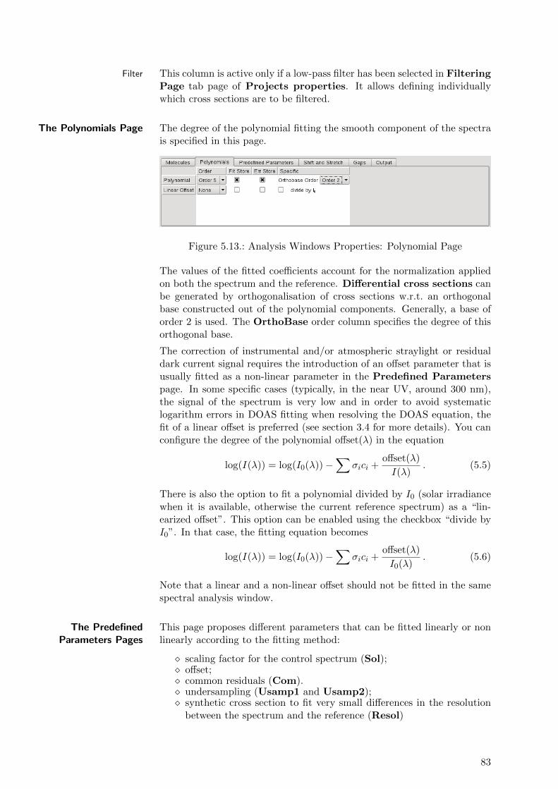
Filter This column is active only if a low-pass filter has been selected in FilteringPage tab page of Projects properties. It allows defining individuallywhich cross sections are to be filtered.
The Polynomials Page The degree of the polynomial fitting the smooth component of the spectrais specified in this page.
Figure 5.13.: Analysis Windows Properties: Polynomial Page
The values of the fitted coefficients account for the normalization appliedon both the spectrum and the reference. Differential cross sections canbe generated by orthogonalisation of cross sections w.r.t. an orthogonalbase constructed out of the polynomial components. Generally, a base oforder 2 is used. The OrthoBase order column specifies the degree of thisorthogonal base.
The correction of instrumental and/or atmospheric straylight or residualdark current signal requires the introduction of an offset parameter that isusually fitted as a non-linear parameter in the Predefined Parameterspage. In some specific cases (typically, in the near UV, around 300 nm),the signal of the spectrum is very low and in order to avoid systematiclogarithm errors in DOAS fitting when resolving the DOAS equation, thefit of a linear offset is preferred (see section 3.4 for more details). You canconfigure the degree of the polynomial offset(λ) in the equation
log(I(λ)) = log(I0(λ))−∑
σici +offset(λ)
I(λ). (5.5)
There is also the option to fit a polynomial divided by I0 (solar irradiancewhen it is available, otherwise the current reference spectrum) as a “lin-earized offset”. This option can be enabled using the checkbox “divide byI0”. In that case, the fitting equation becomes
log(I(λ)) = log(I0(λ))−∑
σici +offset(λ)
I0(λ). (5.6)
Note that a linear and a non-linear offset should not be fitted in the samespectral analysis window.
The PredefinedParameters Pages
This page proposes different parameters that can be fitted linearly or nonlinearly according to the fitting method:
� scaling factor for the control spectrum (Sol);� offset;� common residuals (Com).� undersampling (Usamp1 and Usamp2);� synthetic cross section to fit very small differences in the resolution
between the spectrum and the reference (Resol)
83
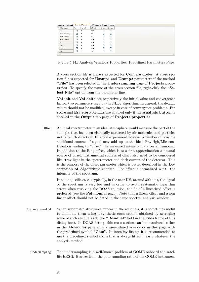
Figure 5.14.: Analysis Windows Properties: Predefined Parameters Page
A cross section file is always expected for Com parameter. A cross sec-tion file is expected for Usamp1 and Usamp2 parameters if the method“File” has been selected in the Undersampling page of Projects prop-erties. To specify the name of the cross section file, right-click the “Se-lect File” option from the parameter line.
Val init and Val delta are respectively the initial value and convergencefactor, two parameters used by the NLLS algorithm. In general, the defaultvalues should not be modified, except in case of convergence problems. Fitstore and Err store columns are enabled only if the Analysis button ischecked in the Output tab page of Projects properties.
Offset An ideal spectrometer in an ideal atmosphere would measure the part of thesunlight that has been elastically scattered by air molecules and particlesin the zenith direction. In a real experiment however a number of possibleadditional sources of signal may add up to the ideal Rayleigh/Mie con-tribution leading to “offset” the measured intensity by a certain amount.In addition to the Ring effect, which is to a first approximation a naturalsource of offset, instrumental sources of offset also need to be consideredlike stray light in the spectrometer and dark current of the detector. Thisis the purpose of the offset parameter which is better described in the De-scription of Algorithms chapter. The offset is normalized w.r.t. theintensity of the spectrum.
In some specific cases (typically, in the near UV, around 300 nm), the signalof the spectrum is very low and in order to avoid systematic logarithmerrors when resolving the DOAS equation, the fit of a linearized offset ispreferred (see the Polynomial page). Note that a linear offset and a nonlinear offset should not be fitted in the same spectral analysis window.
Common residual When systematic structures appear in the residuals, it is sometimes usefulto eliminate them using a synthetic cross section obtained by averagingsome of such residuals (cfr the “Residual” field in the Files frame of thisdialog box). In DOAS fitting, this cross section can be introduced eitherin the Molecules page with a user-defined symbol or in this page withthe predefined symbol “Com”. In intensity fitting, it is recommended touse the predefined symbol Com that is always fitted linearly whatever theanalysis method.
Undersampling The undersampling is a well-known problem of GOME onboard the satel-lite ERS-2. It arises from the poor sampling ratio of the GOME instrument
84

(2 to 3 pixels/FWHM of the resolution of the spectrometer) which resultsin a lost of spectral information when interpolating earthshine spectra dur-ing the DOAS fitting process. The problem can be corrected using ad-hoccross sections obtained by simulating the effect from a high-resolution so-lar reference. If the fit button of Usamp 1 and/or Usamp 2 items ischecked, the options of the Undersampling page of Project properties(cfr page 67) are used to calculate undersampling cross sections. In Fromfile method, undersampling cross sections can be pre-calculated using theQDOAS undersampling tool.
Resol synthetic cross section This cross section is built automatically by dividing the selected referencespectrum with itself but convolved with a gaussian with a FWHM of 0.05nm. It allows accounting for very small differences in the resolution of thereference spectrum and the spectrum to analyze.
The Shift and StretchPage
Shift and stretch parameters allow correcting for possible misalignmentbetween the various spectral items involved in the data evaluation (i.e.measured and reference spectra as well as absorption cross sections). Theequation below gives the wavelength transformation to apply when a shiftand a stretch order 2 are fitted:
∆ = a+ b.(λ− λ0) + c.(λ− λ0)2 (5.7)
Less used, the scaling parameter consists in a wavelength dependent scalingfactor to apply to a cross section. It can also be order 1 or order 2.
Figure 5.15.: Analysis Windows Properties: Shift and Stretch Page
To add an item to shift, stretch or scale, right-click the Insert optionto open a dialog box with the list of available symbols (all cross sectionsdefined in the Molecules page and completed with Spectrum and Refsymbols). It is possible to select only one or several symbols. In the lattercase, the same shift and stretch parameters will be applied to all items of theselection (in the example above, the same shift and stretch will be appliedon both NO2 cross sections). After the validation of the selection, QDOASautomatically updates the list of available symbols so that a symbol cannot be selected twice.
Note that a symbol can not be removed from the Molecules page as longas it is used in the Shift and Stretch page.
85
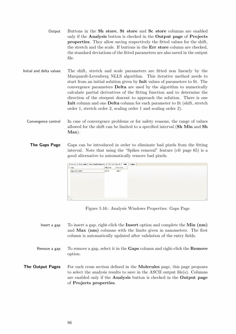
Output Buttons in the Sh store, St store and Sc store columns are enabledonly if the Analysis button is checked in the Output page of Projectsproperties. They allow saving respectively the fitted values for the shift,the stretch and the scale. If buttons in the Err store column are checked,the standard deviations of the fitted parameters are also saved in the outputfile.
Initial and delta values The shift, stretch and scale parameters are fitted non linearly by theMarquardt-Levenberg NLLS algorithm. This iterative method needs tostart from an initial solution given by Init values of parameters to fit. Theconvergence parameters Delta are used by the algorithm to numericallycalculate partial derivatives of the fitting function and to determine thedirection of the steepest descent to approach the solution. There is oneInit column and one Delta column for each parameter to fit (shift, stretchorder 1, stretch order 2, scaling order 1 and scaling order 2).
Convergence control In case of convergence problems or for safety reasons, the range of valuesallowed for the shift can be limited to a specified interval (Sh Min and ShMax).
The Gaps Page Gaps can be introduced in order to eliminate bad pixels from the fittinginterval. Note that using the “Spikes removal” feature (cfr page 65) is agood alternative to automatically remove bad pixels.
Figure 5.16.: Analysis Windows Properties: Gaps Page
Insert a gap To insert a gap, right-click the Insert option and complete the Min (nm)and Max (nm) columns with the limits given in nanometers. The firstcolumn is automatically updated after validation of the entry fields.
Remove a gap To remove a gap, select it in the Gaps column and right-click the Removeoption.
The Output Pages For each cross section defined in the Molecules page, this page proposesto select the analysis results to save in the ASCII output file(s). Columnsare enabled only if the Analysis button is checked in the Output pageof Projects properties.
86
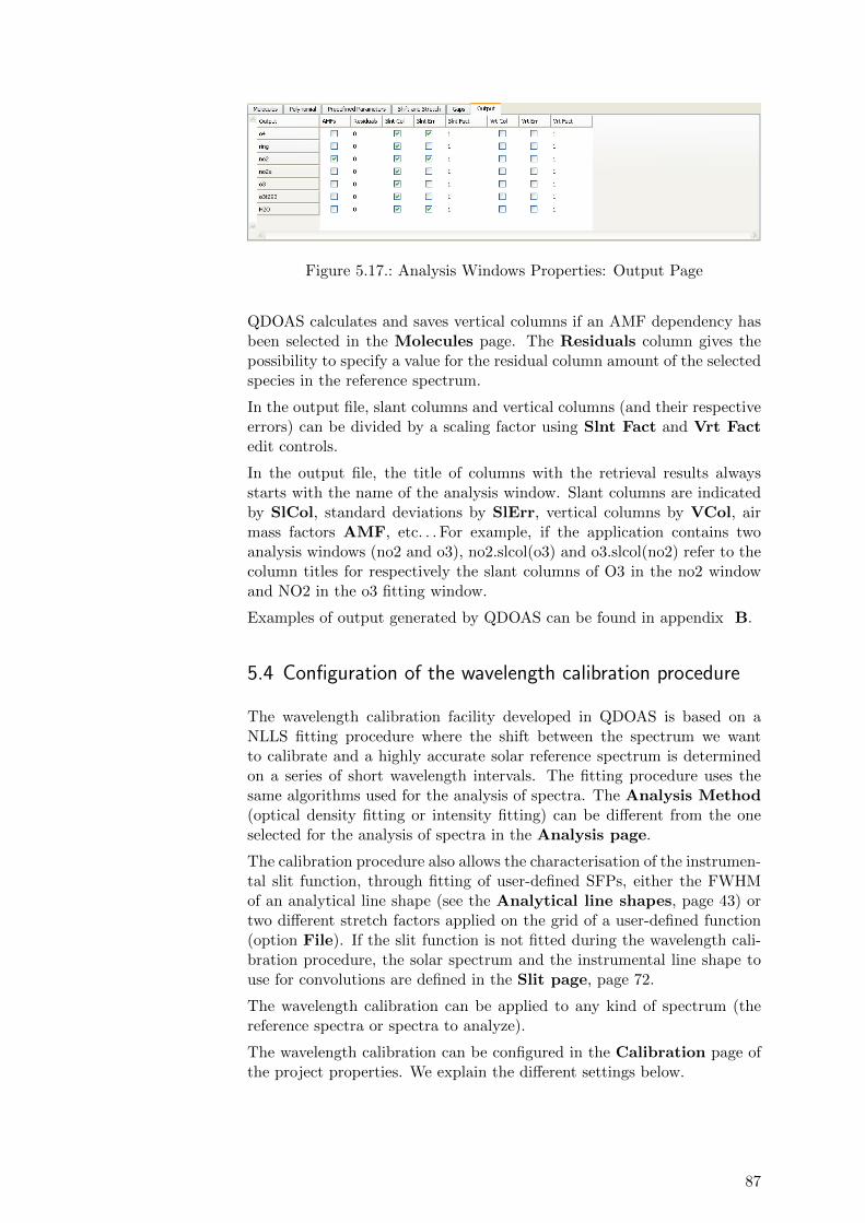
Figure 5.17.: Analysis Windows Properties: Output Page
QDOAS calculates and saves vertical columns if an AMF dependency hasbeen selected in the Molecules page. The Residuals column gives thepossibility to specify a value for the residual column amount of the selectedspecies in the reference spectrum.
In the output file, slant columns and vertical columns (and their respectiveerrors) can be divided by a scaling factor using Slnt Fact and Vrt Factedit controls.
In the output file, the title of columns with the retrieval results alwaysstarts with the name of the analysis window. Slant columns are indicatedby SlCol, standard deviations by SlErr, vertical columns by VCol, airmass factors AMF, etc. . . For example, if the application contains twoanalysis windows (no2 and o3), no2.slcol(o3) and o3.slcol(no2) refer to thecolumn titles for respectively the slant columns of O3 in the no2 windowand NO2 in the o3 fitting window.
Examples of output generated by QDOAS can be found in appendix B.
5.4 Configuration of the wavelength calibration procedure
The wavelength calibration facility developed in QDOAS is based on aNLLS fitting procedure where the shift between the spectrum we wantto calibrate and a highly accurate solar reference spectrum is determinedon a series of short wavelength intervals. The fitting procedure uses thesame algorithms used for the analysis of spectra. The Analysis Method(optical density fitting or intensity fitting) can be different from the oneselected for the analysis of spectra in the Analysis page.
The calibration procedure also allows the characterisation of the instrumen-tal slit function, through fitting of user-defined SFPs, either the FWHMof an analytical line shape (see the Analytical line shapes, page 43) ortwo different stretch factors applied on the grid of a user-defined function(option File). If the slit function is not fitted during the wavelength cali-bration procedure, the solar spectrum and the instrumental line shape touse for convolutions are defined in the Slit page, page 72.
The wavelength calibration can be applied to any kind of spectrum (thereference spectra or spectra to analyze).
The wavelength calibration can be configured in the Calibration page ofthe project properties. We explain the different settings below.
87

Figure 5.18.: Projects properties: Calibration page
Solar Reference Fileand Line Shape
There are two cases to consider:
1. The slit function (line shape) of the instrument is known and thereis no need to characterise it once again (Line Shape “Don’t fit”).Then the Solar Ref. File in this page is disabled; it should be givenin the Slit page, together with the known instrumental line shape.
2. The slit function of the instrument needs to be characterized (se-lection of a Line Shape): the Solar Ref. File should contain ahigh-resolution solar spectrum. Because the convolution algorithmin QDOAS uses the Fourier transform to speed up the NLLS fit-ting, a high-resolution solar spectrum sampled on a constant grid isexpected.
Display When the calibration procedure is applied, a page named “Kurucz” appearsin the plot area of the program except if the Calibration fits button isunchecked in the Display page. This page includes four kinds of plots:
Spectra the complete fit between the observed and the calculated spectra;
Fits fit of the Ring effect and/or atmospheric absorptions if any;
Residual the residual of the fit;
Shift/SFP the wavelength dependency of the shift and the slit functionparameters over the whole detector.
Polynomial Degree When the fitting procedure for each subwindow has finished, a polynomialis used to approximate the shift values determined in each subwindow.This polynomial is then used to correct the initial wavelength calibration.Similarly, the wavelength dependent slit function is determined by fittinga polynomial through the individual SFP values. A different polynomialdegree can be specified for the shift and for the slit function. The wave-length calibration and the variation of the slit function thus determined arethen used e.g. to convolve high resolution cross sections before the analysisof spectra and to build undersampling cross sections.
88

Calibration Interval The wavelength interval used for the calibration must be specified in theCalib. Interval (nm) frame. It should cover all the spectral analysiswindows defined under the Analysis Windows node of the projects tree.This calibration interval is divided in a number of subwindows and theshift and the SFPs are fitted using the NLLS approach within each of thesesubwindows. The settings in the frame Calibration windows control thedefinition of these subwindows.
Calibration Windows During the calibration procedure, the calibration interval is divided into anumber of smaller intervals. The settings in the Calibration Windowsframe can be used to define these intervals. The user can set the number ofintervals to be used, and set their limits using one of the following optionsfrom the Subdivision drop-down menu:
Contiguous With the default “Contiguous” option, the complete calibra-tion interval is divided into non-overlapping subwindows of equal size.
Sliding The more general “Sliding” option allows the user to choose thewidth of the subwindows (“Size (nm)”), independently from the num-ber of subwindows. The calibration interval is now divided into anumber of equally spaced subwindows, which can be made to overlapby choosing a larger size, or made disjoint by choosing a smaller size.Usually, one wants to increase the size of the subwindows in order toimprove the stability of the calibration fit in each subwindow.
Custom With the “Custom” option, the user can manually set the limits ofthe subintervals used in the calibration. Clicking on the “Define win-dows” button opens a pop-up where the lower and upper wavelengthlimit can be configured for each subwindow.
Fitting Parameters The wavelength calibration uses a similar property sheet as the Analysiswindows properties to configure the fitting procedure for the calibrationsubwindows. The configuration of these pages is usually limited to thespecification of the degree of the polynomial uses in the DOAS equation(different from the polynomial used to build the final grid from the indi-vidual values of the shift resulting from the fit as described above), theslit function parameters to fit according to the selection of the line shapeand the shift between the spectrum to calibrate and the solar spectrum.But the algorithm can also take into account atmospheric absorption, Ringeffect and offset correction.
The Molecules page The Molecules page allows introducing correcting absorbers that mayoptimise the accuracy of the wavelength calibration, e.g. the Ring effect(when calibrating a scattered-light spectrum) and O3 absorption can betaken into account in the fit.
To generate differential cross sections (column Diff/Orthog), see page 80.The Fit display column is activated only if the Calibration button ischecked in the Display page of Projects properties (see page 62) and ifthe Fits button is checked in the Display frame of the Calibration page(see page 67). The selected cross section are usually pre-convolved withthe resolution of the instrument and interpolated on the grid of the control(reference) spectrum.
89
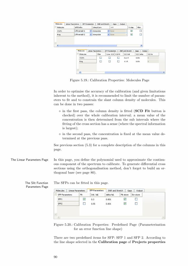
Figure 5.19.: Calibration Properties: Molecules Page
In order to optimise the accuracy of the calibration (and given limitationsinherent to the method), it is recommended to limit the number of param-eters to fit and to constrain the slant column density of molecules. Thiscan be done in two passes:
� in the first pass, the column density is fitted (SCD Fit button ischecked) over the whole calibration interval; a mean value of theconcentration is then determined from the sub intervals where thefitting of the cross section has a sense (where the spectral informationis largest);
� in the second pass, the concentration is fixed at the mean value de-termined at the previous pass.
See previous section (5.3) for a complete description of the columns in thispage.
The Linear Parameters Page In this page, you define the polynomial used to approximate the continu-ous component of the spectrum to calibrate. To generate differential crosssections using the orthogonalisation method, don’t forget to build an or-thogonal base (see page 80).
The Slit FunctionParameters Page
The SFPs can be fitted in this page.
Figure 5.20.: Calibration Properties: Predefined Page (Parameterisationfor an error function line shape)
There are two predefined items for SFP: SFP 1 and SFP 2. According tothe line shape selected in the Calibration page of Projects properties
90
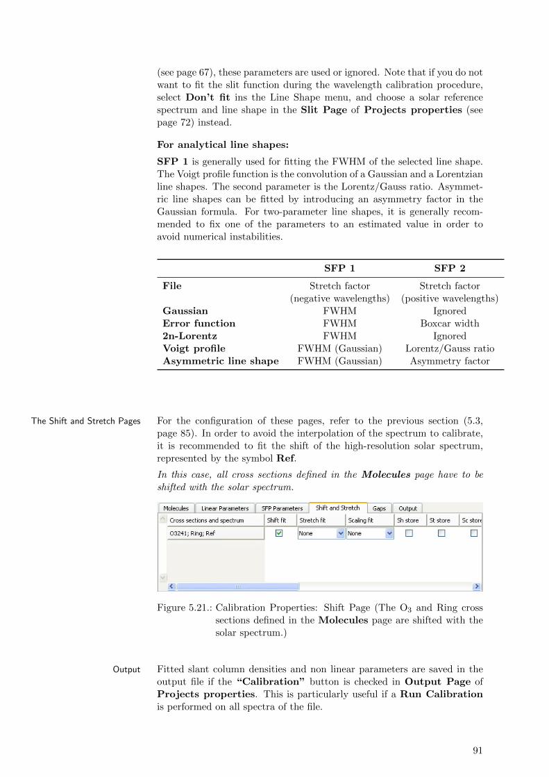
(see page 67), these parameters are used or ignored. Note that if you do notwant to fit the slit function during the wavelength calibration procedure,select Don’t fit ins the Line Shape menu, and choose a solar referencespectrum and line shape in the Slit Page of Projects properties (seepage 72) instead.
For analytical line shapes:
SFP 1 is generally used for fitting the FWHM of the selected line shape.The Voigt profile function is the convolution of a Gaussian and a Lorentzianline shapes. The second parameter is the Lorentz/Gauss ratio. Asymmet-ric line shapes can be fitted by introducing an asymmetry factor in theGaussian formula. For two-parameter line shapes, it is generally recom-mended to fix one of the parameters to an estimated value in order toavoid numerical instabilities.
SFP 1 SFP 2
File Stretch factor Stretch factor(negative wavelengths) (positive wavelengths)
Gaussian FWHM IgnoredError function FWHM Boxcar width2n-Lorentz FWHM IgnoredVoigt profile FWHM (Gaussian) Lorentz/Gauss ratioAsymmetric line shape FWHM (Gaussian) Asymmetry factor
The Shift and Stretch Pages For the configuration of these pages, refer to the previous section (5.3,page 85). In order to avoid the interpolation of the spectrum to calibrate,it is recommended to fit the shift of the high-resolution solar spectrum,represented by the symbol Ref.
In this case, all cross sections defined in the Molecules page have to beshifted with the solar spectrum.
Figure 5.21.: Calibration Properties: Shift Page (The O3 and Ring crosssections defined in the Molecules page are shifted with thesolar spectrum.)
Output Fitted slant column densities and non linear parameters are saved in theoutput file if the “Calibration” button is checked in Output Page ofProjects properties. This is particularly useful if a Run Calibrationis performed on all spectra of the file.
91
Calculation of thepreshift
If the wavelength calibration of the reference spectrum is really too bad,the calibration procedure couldn’t converge and return a wrong value ofthe shift that corresponds to a local minimum of the chi square. In thiscase, it could be useful to approximate the value of the shift by calculatingthe correlation between the reference spectrum and the solar spectrumconvolved at the resolution of the instrument using the initial value(s)of the slit function parameter(s). The value of the shift giving the bestcorrelation will be introduced by the program as initial shift of the usualNLLS algorithm. To calculate the preshift before the Kurucz procedure,check the “Calculate preshift” button in the “Preshift (nm)” frameand define the interval in nanometers wherein the shift values can vary forthe correlation test.
92
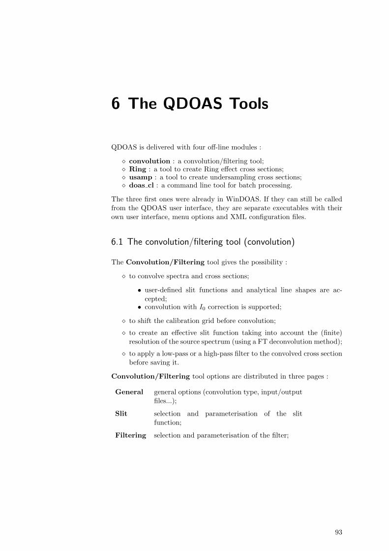
6 The QDOAS Tools
QDOAS is delivered with four off-line modules :
� convolution : a convolution/filtering tool;� Ring : a tool to create Ring effect cross sections;� usamp : a tool to create undersampling cross sections;� doas cl : a command line tool for batch processing.
The three first ones were already in WinDOAS. If they can still be calledfrom the QDOAS user interface, they are separate executables with theirown user interface, menu options and XML configuration files.
6.1 The convolution/filtering tool (convolution)
The Convolution/Filtering tool gives the possibility :
� to convolve spectra and cross sections;
• user-defined slit functions and analytical line shapes are ac-cepted;
• convolution with I0 correction is supported;
� to shift the calibration grid before convolution;
� to create an effective slit function taking into account the (finite)resolution of the source spectrum (using a FT deconvolution method);
� to apply a low-pass or a high-pass filter to the convolved cross sectionbefore saving it.
Convolution/Filtering tool options are distributed in three pages :
General general options (convolution type, input/outputfiles...);
Slit selection and parameterisation of the slitfunction;
Filtering selection and parameterisation of the filter;
93
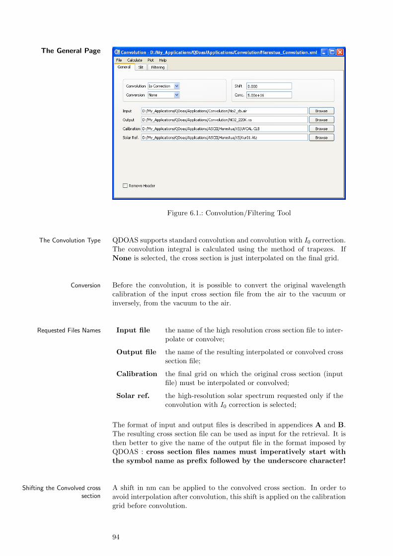
The General Page
Figure 6.1.: Convolution/Filtering Tool
The Convolution Type QDOAS supports standard convolution and convolution with I0 correction.The convolution integral is calculated using the method of trapezes. IfNone is selected, the cross section is just interpolated on the final grid.
Conversion Before the convolution, it is possible to convert the original wavelengthcalibration of the input cross section file from the air to the vacuum orinversely, from the vacuum to the air.
Requested Files Names Input file the name of the high resolution cross section file to inter-polate or convolve;
Output file the name of the resulting interpolated or convolved crosssection file;
Calibration the final grid on which the original cross section (inputfile) must be interpolated or convolved;
Solar ref. the high-resolution solar spectrum requested only if theconvolution with I0 correction is selected;
The format of input and output files is described in appendices A and B.The resulting cross section file can be used as input for the retrieval. It isthen better to give the name of the output file in the format imposed byQDOAS : cross section files names must imperatively start withthe symbol name as prefix followed by the underscore character!
Shifting the Convolved crosssection
A shift in nm can be applied to the convolved cross section. In order toavoid interpolation after convolution, this shift is applied on the calibrationgrid before convolution.
94
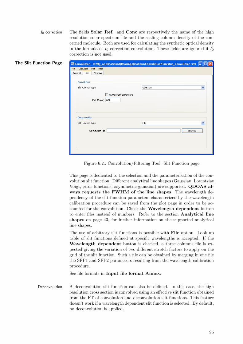
I0 correction The fields Solar Ref. and Conc are respectively the name of the highresolution solar spectrum file and the scaling column density of the con-cerned molecule. Both are used for calculating the synthetic optical densityin the formula of I0 correction convolution. These fields are ignored if I0
correction is not used.
The Slit Function Page
Figure 6.2.: Convolution/Filtering Tool: Slit Function page
This page is dedicated to the selection and the parameterisation of the con-volution slit function. Different analytical line shapes (Gaussian, Lorentzian,Voigt, error functions, asymmetric gaussian) are supported. QDOAS al-ways requests the FWHM of the line shapes. The wavelength de-pendency of the slit function parameters characterized by the wavelengthcalibration procedure can be saved from the plot page in order to be ac-counted for the convolution. Check the Wavelength dependent buttonto enter files instead of numbers. Refer to the section Analytical lineshapes on page 43, for further information on the supported analyticalline shapes.
The use of arbitrary slit functions is possible with File option. Look uptable of slit functions defined at specific wavelengths is accepted. If theWavelength dependent button is checked, a three columns file is ex-pected giving the variation of two different stretch factors to apply on thegrid of the slit function. Such a file can be obtained by merging in one filethe SFP1 and SFP2 parameters resulting from the wavelength calibrationprocedure.
See file formats in Input file format Annex.
Deconvolution A deconvolution slit function can also be defined. In this case, the highresolution cross section is convolved using an effective slit function obtainedfrom the FT of convolution and deconvolution slit functions. This featuredoesn’t work if a wavelength dependent slit function is selected. By default,no deconvolution is applied.
95
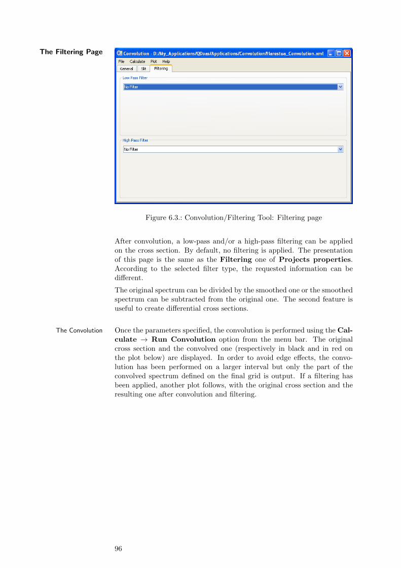
The Filtering Page
Figure 6.3.: Convolution/Filtering Tool: Filtering page
After convolution, a low-pass and/or a high-pass filtering can be appliedon the cross section. By default, no filtering is applied. The presentationof this page is the same as the Filtering one of Projects properties.According to the selected filter type, the requested information can bedifferent.
The original spectrum can be divided by the smoothed one or the smoothedspectrum can be subtracted from the original one. The second feature isuseful to create differential cross sections.
The Convolution Once the parameters specified, the convolution is performed using the Cal-culate → Run Convolution option from the menu bar. The originalcross section and the convolved one (respectively in black and in red onthe plot below) are displayed. In order to avoid edge effects, the convo-lution has been performed on a larger interval but only the part of theconvolved spectrum defined on the final grid is output. If a filtering hasbeen applied, another plot follows, with the original cross section and theresulting one after convolution and filtering.
96

Figure 6.4.: Convolution with I0 correction of a NO2 cross section with aGaussian (FWHM : 0.5 nm) [27]
6.2 The Ring tool (ring)
The so-called Ring effect arises in the atmosphere due to inelastic scatter-ing processes (mainly RRS by molecular O2 and N2). Roughly speaking,it manifests itself by a broadening of the solar and atmospheric spectralfeatures present in measured spectra. This broadening typically reducesthe depth of thin solar and atmospheric absorption features by several per-cents. Hence, it has a strong impact on spectroscopic measurements usingthe DOAS method and retrieval algorithms must appropriately correct forit. This is especially true for minor absorbers like BrO or OClO, for whichweak absorption features can be completely masked by Ring structures.
In DOAS, the Ring effect is usually accounted for as an absorber. TheQDOAS Ring tool calculates Ring cross sections using a simple methoddescribed by Chance and Spurr [9]. See the Description of Algorithmschapter, page 35 for further information on the Ring effect.
97
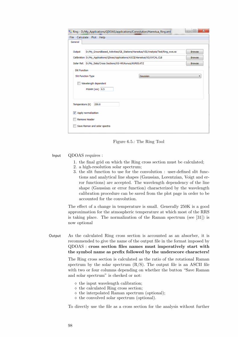
Figure 6.5.: The Ring Tool
Input QDOAS requires :
1. the final grid on which the Ring cross section must be calculated;2. a high-resolution solar spectrum;3. the slit function to use for the convolution : user-defined slit func-
tions and analytical line shapes (Gaussian, Lorentzian, Voigt and er-ror functions) are accepted. The wavelength dependency of the lineshape (Gaussian or error function) characterized by the wavelengthcalibration procedure can be saved from the plot page in order to beaccounted for the convolution.
The effect of a change in temperature is small. Generally 250K is a goodapproximation for the atmospheric temperature at which most of the RRSis taking place. The normalization of the Raman spectrum (see [31]) isnow optional
Output As the calculated Ring cross section is accounted as an absorber, it isrecommended to give the name of the output file in the format imposed byQDOAS : cross section files names must imperatively start withthe symbol name as prefix followed by the underscore characters!
The Ring cross section is calculated as the ratio of the rotational Ramanspectrum by the solar spectrum (R/S). The output file is an ASCII filewith two or four columns depending on whether the button “Save Ramanand solar spectrum” is checked or not:
� the input wavelength calibration;� the calculated Ring cross section;� the interpolated Raman spectrum (optional);� the convolved solar spectrum (optional).
To directly use the file as a cross section for the analysis without further
98

convolution, only the first two columns should be saved (the program willdisplay an error if the file contains unneeded columns). If the ConvolveRing action is requested (see the Molecules page of Analysis windowsproperties), the program needs all four columns. With “Convolve Ring”,QDOAS uses the information on the slit function retrieved from the wave-length calibration procedure or from the slit function page to convolve theRaman and the solar spectra separately, and use the calculated ratio as aRing cross section in the fit.
Figure 6.6.: Ring cross section generated with the Ring Tool
6.3 The undersampling tool (usamp)
The undersampling is a well-known problem of GOME onboard the satelliteERS-2. It arises from the poor sampling ratio of the GOME instrument (2to 3 pixels/FWHM of the resolution of the spectrometer) which results ina lost of spectral information when interpolating earthshine spectra duringthe DOAS fitting process. The problem can be corrected using ad-hoccross sections obtained by simulating the effect from a high-resolution solarreference (see Chance K., 1998 [7]).
The approach consists in building two spectra (an oversampled one and anundersampled one) from the high resolution solar spectrum and accordingto the selected analysis method, to calculate the ratio (DOAS fitting) orthe difference (Intensity fitting) in order to simulate the interpolation error.Two undersampling cross sections are generated (the first one using theinstrument grid and the second one using the instrument grid with a smallshift applied).
See the Description of Algorithms chapter, page 36, for further infor-mation on the undersampling.
99
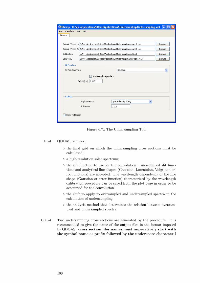
Figure 6.7.: The Undersampling Tool
Input QDOAS requires :
� the final grid on which the undersampling cross sections must becalculated;
� a high-resolution solar spectrum;
� the slit function to use for the convolution : user-defined slit func-tions and analytical line shapes (Gaussian, Lorentzian, Voigt and er-ror functions) are accepted. The wavelength dependency of the lineshape (Gaussian or error function) characterized by the wavelengthcalibration procedure can be saved from the plot page in order to beaccounted for the convolution.
� the shift to apply to oversampled and undersampled spectra in thecalculation of undersampling;
� the analysis method that determines the relation between oversam-pled and undersampled spectra;
Output Two undersampling cross sections are generated by the procedure. It isrecommended to give the name of the output files in the format imposedby QDOAS : cross section files names must imperatively start withthe symbol name as prefix followed by the underscore character !
100
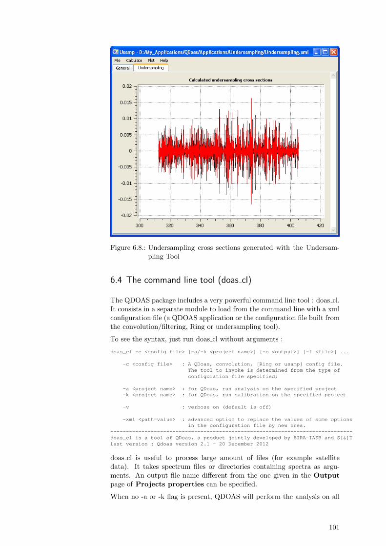
Figure 6.8.: Undersampling cross sections generated with the Undersam-pling Tool
6.4 The command line tool (doas cl)
The QDOAS package includes a very powerful command line tool : doas cl.It consists in a separate module to load from the command line with a xmlconfiguration file (a QDOAS application or the configuration file built fromthe convolution/filtering, Ring or undersampling tool).
To see the syntax, just run doas cl without arguments :
doas_cl -c <config file> [-a/-k <project name>] [-o <output>] [-f <file>] ...
-c <config file> : A QDoas, convolution, [Ring or usamp] config file.The tool to invoke is determined from the type ofconfiguration file specified;
-a <project name> : for QDoas, run analysis on the specified project-k <project name> : for QDoas, run calibration on the specified project
-v : verbose on (default is off)
-xml <path=value> : advanced option to replace the values of some optionsin the configuration file by new ones.
------------------------------------------------------------------------------doas_cl is a tool of QDoas, a product jointly developed by BIRA-IASB and S[&]TLast version : Qdoas version 2.1 - 20 December 2012
doas cl is useful to process large amount of files (for example satellitedata). It takes spectrum files or directories containing spectra as argu-ments. An output file name different from the one given in the Outputpage of Projects properties can be specified.
When no -a or -k flag is present, QDOAS will perform the analysis on all
101
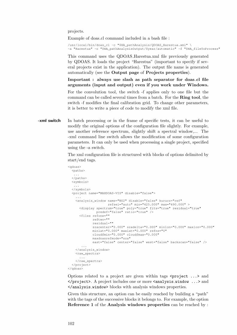
projects.
Example of doas cl command included in a bash file :
/usr/local/bin/doas_cl -c "$HA_pathAnalysis/QDOAS_Harestua.xml" \-a "Harestua" -o "$HA_pathAnalysisOutput/$year/automatic" -f "$HA_fileToProcess"
This command uses the QDOAS Harestua.xml file previously generatedby QDOAS. It loads the project “Harestua” (important to specify if sev-eral projects exist in the application). The output file name is generatedautomatically (see the Output page of Projects properties).
Important : always use slash as path separator for doas cl filearguments (input and output) even if you work under Windows.
For the convolution tool, the switch -f applies only to one file but thecommand can be called several times from a batch. For the Ring tool, theswitch -f modifies the final calibration grid. To change other parameters,it is better to write a piece of code to modify the xml file.
-xml switch In batch processing or in the frame of specific tests, it can be useful tomodify the original options of the configuration file slightly. For example,use another reference spectrum, slightly shift a spectral window,... The-xml command line switch allows the modification of some configurationparameters. It can only be used when processing a single project, specifiedusing the -a switch.
The xml configuration file is structured with blocks of options delimited bystart/end tags.
<qdoas><paths>...</paths><symbols>...</symbols><project name="MAXDOAS-VIS" disable="false">...<analysis_window name="NO2" disable="false" kurucz="ref"
refsel="auto" min="425.000" max="490.000" ><display spectrum="true" poly="true" fits="true" residual="true"
predef="false" ratio="true" /><files refone=""
reftwo=""residual=""szacenter="0.000" szadelta="0.000" minlon="0.000" maxlon="0.000"minlat="0.000" maxlat="0.000" refns="0"cloudfmin="0.000" cloudfmax="0.000"maxdoasrefmode="sza"east="false" center="false" west="false" backscan="false" />
...</analysis_window><raw_spectra>...
</raw_spectra></project>
</qdoas>
Options related to a project are given within tags <project ...> and</project>. A project includes one or more <analysis window ...> and</analysis window> blocks with analysis windows properties.
Given this structure, an option can be easily reached by building a “path”with the tags of the successive blocks it belongs to. For example, the optionReference 1 of the Analysis windows properties can be reached by :
102

/project/analysis_window/files/refone
To use a reference file other the one specified in the xml file, the switch-xml in the doas cl command can be used as follows :
-xml "/project/analysis_window/files/refone=<new file>"
It is recommended to quote the whole command. If the name of the anal-ysis window is specified, the changes are applied only on this window.Otherwise, they will be applied to all analysis windows of the project.
To modify the spectra range of the analysis window named NO2, two suc-cessive -xml switches are used :
doas_cl <...> -xml "/project/analysis_window/NO2/min=450"-xml "/project/analysis_window/NO2/max=490"
If the xml command is recognized, the following lines should be displayedon the console :
/project/analysis_window/NO2/min : 425.00 replaced by 450 (NO2)/project/analysis_window/NO2/max : 490.00 replaced by 500 (NO2)
Not all options of the configuration file can be modified. doas cl will indi-cate if a field can not be changed.
103

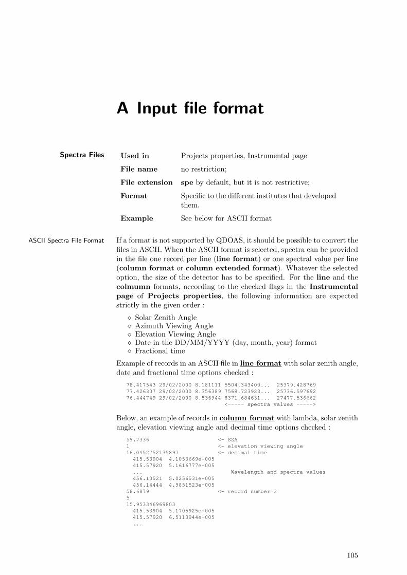
A Input file format
Spectra Files Used in Projects properties, Instrumental page
File name no restriction;
File extension spe by default, but it is not restrictive;
Format Specific to the different institutes that developedthem.
Example See below for ASCII format
ASCII Spectra File Format If a format is not supported by QDOAS, it should be possible to convert thefiles in ASCII. When the ASCII format is selected, spectra can be providedin the file one record per line (line format) or one spectral value per line(column format or column extended format). Whatever the selectedoption, the size of the detector has to be specified. For the line and thecolmumn formats, according to the checked flags in the Instrumentalpage of Projects properties, the following information are expectedstrictly in the given order :
� Solar Zenith Angle� Azimuth Viewing Angle� Elevation Viewing Angle� Date in the DD/MM/YYYY (day, month, year) format� Fractional time
Example of records in an ASCII file in line format with solar zenith angle,date and fractional time options checked :
78.417543 29/02/2000 8.181111 5504.343400... 25379.42876977.426307 29/02/2000 8.356389 7568.723923... 25736.59769276.444749 29/02/2000 8.536944 8371.684631... 27477.536662
<----- spectra values ----->
Below, an example of records in column format with lambda, solar zenithangle, elevation viewing angle and decimal time options checked :
59.7336 <- SZA1 <- elevation viewing angle16.0452752135897 <- decimal time415.53904 4.1053669e+005415.57920 5.1616777e+005... Wavelength and spectra values456.10521 5.0256531e+005456.14444 4.9851523e+005
58.6879 <- record number 2515.953346969803415.53904 5.1705925e+005415.57920 6.5113944e+005...
105

456.10521 6.4016200e+005456.14444 6.3482669e+005
60.4205 <- record number 31016.1055305555417415.53904 5.2111045e+005415.57920 6.5623468e+005...456.10521 6.4077000e+005456.14444 6.3549114e+005
Until version 2.106, angles had to be given on the same line. Now, it is notthe case anymore. Angles had to be given in separate lines and QDOASaccepts matrices of spectra. With the same options checked, the file couldbe :
0 59.7336 58.6879 60.4205 <- SZA0 1 5 10 <- elevation viewing angles0 16.0452752135897 15.953346969803 16.1055305555417 <- decimal times
415.53904 4.1053669e+005 5.1705925e+005 5.2111045e+005415.57920 5.1616777e+005 6.5113944e+005 6.5623468e+005...456.10521 5.0256531e+005 6.4016200e+005 6.4077000e+005456.14444 4.9851523e+005 6.3482669e+005 6.3549114e+005
The wavelength calibration is always provided in the first column. Themaximum number of characters accepted for one line is 4096. The filecan contain successive data blocks but all data blocks should have thesame number of columns. If present, the wavelength calibration has to berepeated the first column of each block.
From version 3.0, QDOAS proposes a Column extended format, moreflexible than the two previous ones. Spectra (preceeded or not by wave-lengths) are provided as column vectors and records can be described by <KEYNAME >=< KEYVALUE > lines where KEYNAMES are the nameof pre-defined fields to choose in the following list according to the type ofmeasurement :
NameDate (DD/MM/YYYY)UTC time (hh:mm:ss)Number of scansExposure TimeSolar Zenith AngleSolar Azimuth AngleLongitudeLatitudeAltitudeViewing elevation angleViewing azimuth angleViewing zenith angleTotal Measurement Time (sec)Total Acquisition Time (sec)Start Date (dd/mm/yyyy)End Date (dd/mm/yyyy)UTC Start Time (hh:mm:ss)UTC End Time (hh:mm:ss)Measurement Type
The file in Column extended format can begin with comment linesstarting with hash character. Exposure time is also called integration time.Total acquisition time should be the exact time needed by the device totake the acquisition of non rejected scans. Total measurement time shouldinclude the overheads requested by the measurement (for example, readingtime, time to calculate the integration time, to move a pointing system...).Spectra exported in ASCII by QDOAS are in Column extended format.
106
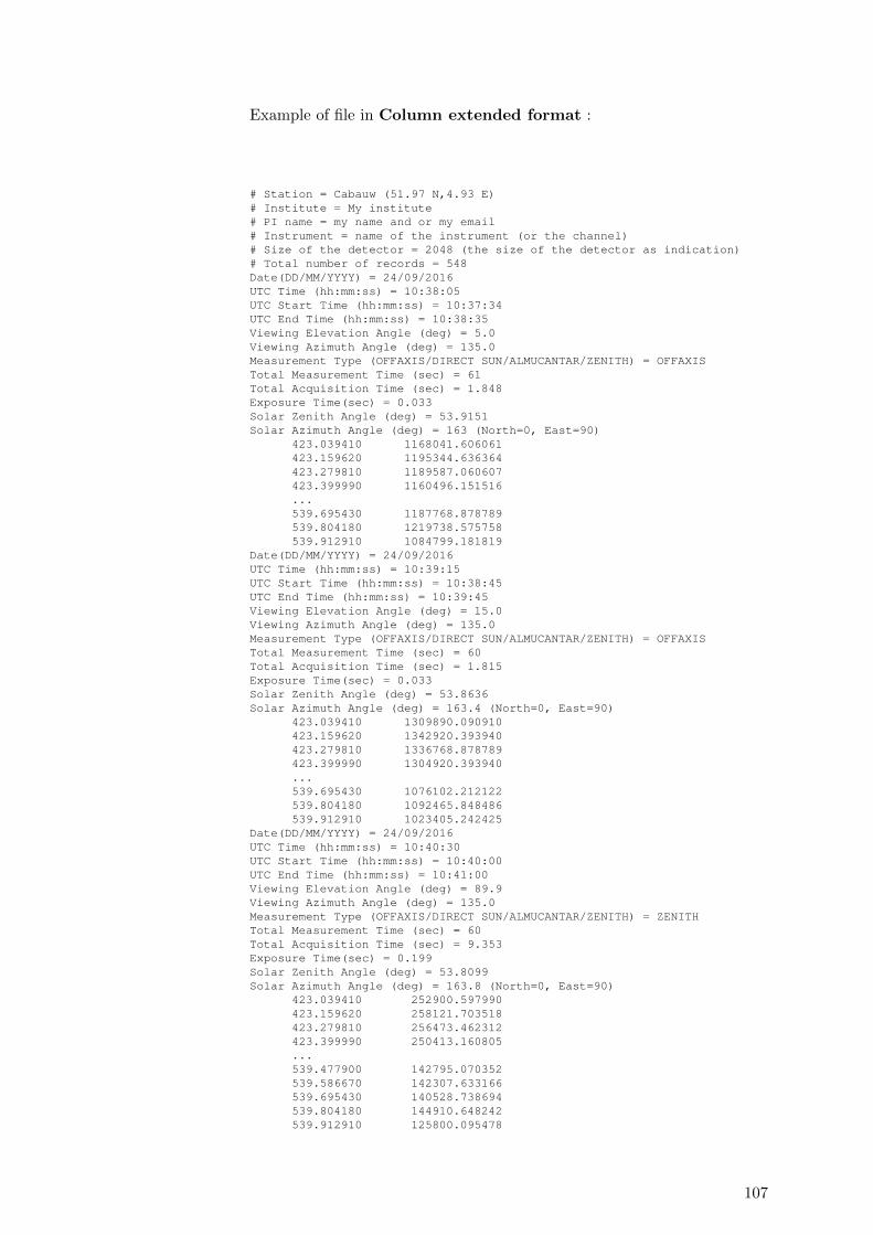
Example of file in Column extended format :
# Station = Cabauw (51.97 N,4.93 E)# Institute = My institute# PI name = my name and or my email# Instrument = name of the instrument (or the channel)# Size of the detector = 2048 (the size of the detector as indication)# Total number of records = 548Date(DD/MM/YYYY) = 24/09/2016UTC Time (hh:mm:ss) = 10:38:05UTC Start Time (hh:mm:ss) = 10:37:34UTC End Time (hh:mm:ss) = 10:38:35Viewing Elevation Angle (deg) = 5.0Viewing Azimuth Angle (deg) = 135.0Measurement Type (OFFAXIS/DIRECT SUN/ALMUCANTAR/ZENITH) = OFFAXISTotal Measurement Time (sec) = 61Total Acquisition Time (sec) = 1.848Exposure Time(sec) = 0.033Solar Zenith Angle (deg) = 53.9151Solar Azimuth Angle (deg) = 163 (North=0, East=90)
423.039410 1168041.606061423.159620 1195344.636364423.279810 1189587.060607423.399990 1160496.151516...539.695430 1187768.878789539.804180 1219738.575758539.912910 1084799.181819
Date(DD/MM/YYYY) = 24/09/2016UTC Time (hh:mm:ss) = 10:39:15UTC Start Time (hh:mm:ss) = 10:38:45UTC End Time (hh:mm:ss) = 10:39:45Viewing Elevation Angle (deg) = 15.0Viewing Azimuth Angle (deg) = 135.0Measurement Type (OFFAXIS/DIRECT SUN/ALMUCANTAR/ZENITH) = OFFAXISTotal Measurement Time (sec) = 60Total Acquisition Time (sec) = 1.815Exposure Time(sec) = 0.033Solar Zenith Angle (deg) = 53.8636Solar Azimuth Angle (deg) = 163.4 (North=0, East=90)
423.039410 1309890.090910423.159620 1342920.393940423.279810 1336768.878789423.399990 1304920.393940...539.695430 1076102.212122539.804180 1092465.848486539.912910 1023405.242425
Date(DD/MM/YYYY) = 24/09/2016UTC Time (hh:mm:ss) = 10:40:30UTC Start Time (hh:mm:ss) = 10:40:00UTC End Time (hh:mm:ss) = 10:41:00Viewing Elevation Angle (deg) = 89.9Viewing Azimuth Angle (deg) = 135.0Measurement Type (OFFAXIS/DIRECT SUN/ALMUCANTAR/ZENITH) = ZENITHTotal Measurement Time (sec) = 60Total Acquisition Time (sec) = 9.353Exposure Time(sec) = 0.199Solar Zenith Angle (deg) = 53.8099Solar Azimuth Angle (deg) = 163.8 (North=0, East=90)
423.039410 252900.597990423.159620 258121.703518423.279810 256473.462312423.399990 250413.160805...539.477900 142795.070352539.586670 142307.633166539.695430 140528.738694539.804180 144910.648242539.912910 125800.095478
107
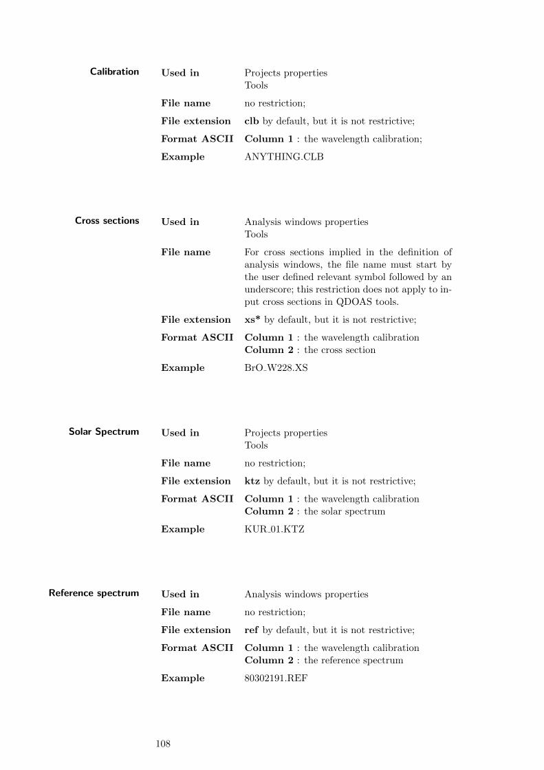
Calibration Used in Projects propertiesTools
File name no restriction;
File extension clb by default, but it is not restrictive;
Format ASCII Column 1 : the wavelength calibration;
Example ANYTHING.CLB
Cross sections Used in Analysis windows propertiesTools
File name For cross sections implied in the definition ofanalysis windows, the file name must start bythe user defined relevant symbol followed by anunderscore; this restriction does not apply to in-put cross sections in QDOAS tools.
File extension xs* by default, but it is not restrictive;
Format ASCII Column 1 : the wavelength calibrationColumn 2 : the cross section
Example BrO W228.XS
Solar Spectrum Used in Projects propertiesTools
File name no restriction;
File extension ktz by default, but it is not restrictive;
Format ASCII Column 1 : the wavelength calibrationColumn 2 : the solar spectrum
Example KUR 01.KTZ
Reference spectrum Used in Analysis windows properties
File name no restriction;
File extension ref by default, but it is not restrictive;
Format ASCII Column 1 : the wavelength calibrationColumn 2 : the reference spectrum
Example 80302191.REF
108
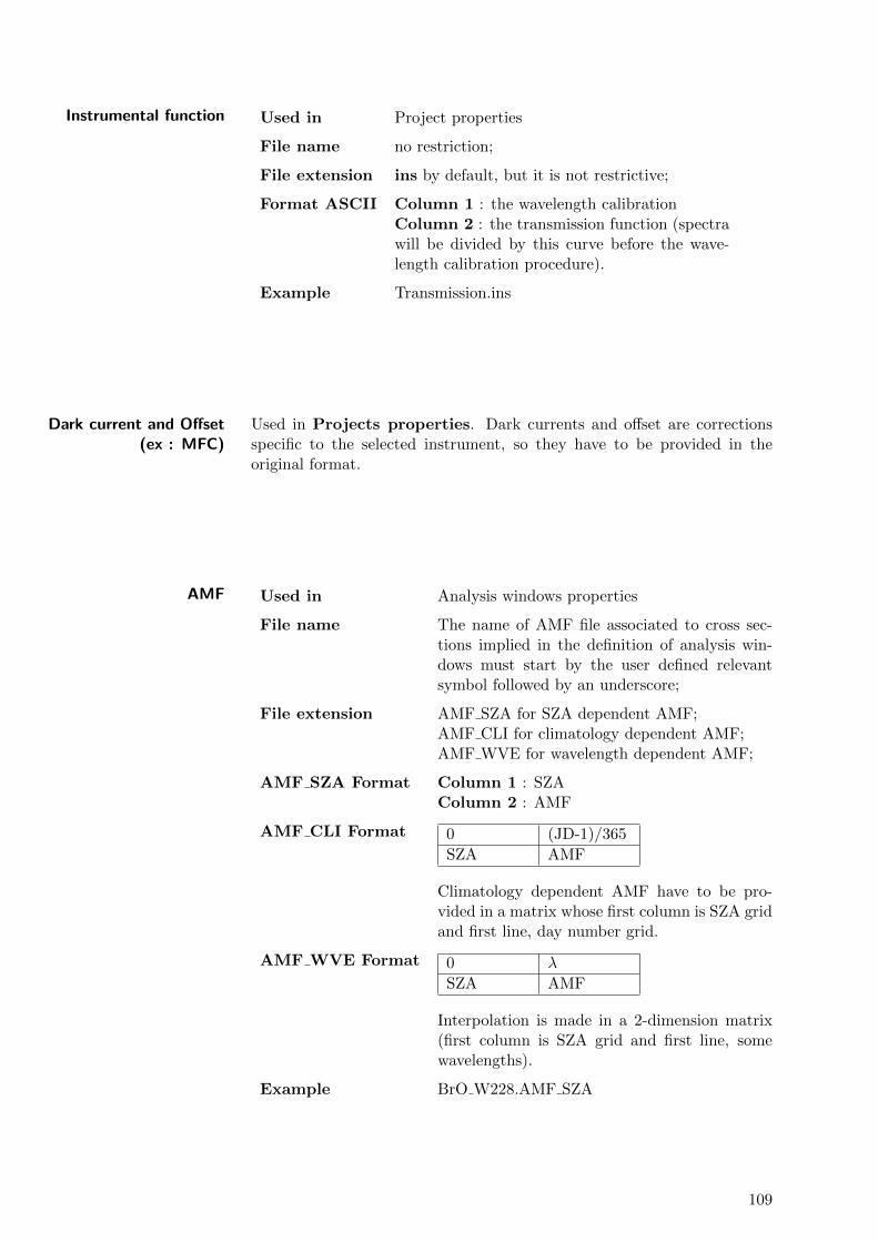
Instrumental function Used in Project properties
File name no restriction;
File extension ins by default, but it is not restrictive;
Format ASCII Column 1 : the wavelength calibrationColumn 2 : the transmission function (spectrawill be divided by this curve before the wave-length calibration procedure).
Example Transmission.ins
Dark current and Offset(ex : MFC)
Used in Projects properties. Dark currents and offset are correctionsspecific to the selected instrument, so they have to be provided in theoriginal format.
AMF Used in Analysis windows properties
File name The name of AMF file associated to cross sec-tions implied in the definition of analysis win-dows must start by the user defined relevantsymbol followed by an underscore;
File extension AMF SZA for SZA dependent AMF;AMF CLI for climatology dependent AMF;AMF WVE for wavelength dependent AMF;
AMF SZA Format Column 1 : SZAColumn 2 : AMF
AMF CLI Format 0 (JD-1)/365
SZA AMF
Climatology dependent AMF have to be pro-vided in a matrix whose first column is SZA gridand first line, day number grid.
AMF WVE Format 0 λ
SZA AMF
Interpolation is made in a 2-dimension matrix(first column is SZA grid and first line, somewavelengths).
Example BrO W228.AMF SZA
109

Slit functions Used in Analysis windows properties
File name no restriction;
File extension slf by default, but it is not restrictive;
Format ASCII Column 1 : the wavelength calibrationColumn 2 : the line shape
The slit function has to be provided with a wavelengthcalibration around 0 nm.
For wavelength dependent slit function types, thesecond column is the parameter dependent on thewavelength.
Since QDOAS version 2.00, lookup tables of wave-length dependent slit functions can be provided. Inthis case, the number of columns depends on the avail-able slit functions. Wavelengths are specified in thefirst line of the file.
Example 0 340 380-1.00 2.9802322387695299e-008 7.8886090522101049e-031-0.98 5.9192925419630987e-008 1.2276631396533808e-029-0.96 1.1594950525907111e-007 1.8074887363782194e-028-0.94 2.2399967890119956e-007 2.5176165401687836e-027...-0.04 9.7265494741228542e-001 8.9502507092797223e-001-0.02 9.9309249543703593e-001 9.7265494741228542e-0010.00 1.0000000000000000e+000 1.0000000000000000e+0000.02 9.9309249543703593e-001 9.7265494741228542e-0010.04 9.7265494741228542e-001 8.9502507092797223e-001
...0.94 2.2399967890119956e-007 2.5176165401687836e-0270.96 1.1594950525907111e-007 1.8074887363782194e-0280.98 5.9192925419630987e-008 1.2276631396533808e-0291.00 2.9802322387695299e-008 7.8886090522101049e-031
Specific case : For wavelength dependent arbitraryslit function files (including lookup tables of slit func-tions), the variation of the two stretch factors to applyon the grid of the line shape is given in a three-columnsfile.
110
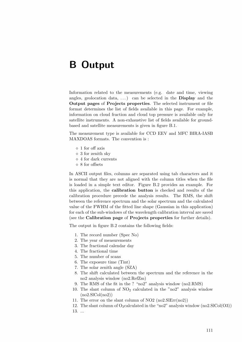
B Output
Information related to the measurements (e.g. date and time, viewingangles, geolocation data, . . . ) can be selected in the Display and theOutput pages of Projects properties. The selected instrument or fileformat determines the list of fields available in this page. For example,information on cloud fraction and cloud top pressure is available only forsatellite instruments. A non-exhaustive list of fields available for ground-based and satellite measurements is given in figure B.1.
The measurement type is available for CCD EEV and MFC BIRA-IASBMAXDOAS formats. The convention is :
� 1 for off axis� 3 for zenith sky� 4 for dark currents� 8 for offsets
In ASCII output files, columns are separated using tab characters and itis normal that they are not aligned with the column titles when the fileis loaded in a simple text editor. Figure B.2 provides an example. Forthis application, the calibration button is checked and results of thecalibration procedure precede the analysis results. The RMS, the shiftbetween the reference spectrum and the solar spectrum and the calculatedvalue of the FWHM of the fitted line shape (Gaussian in this application)for each of the sub-windows of the wavelength calibration interval are saved(see the Calibration page of Projects properties for further details).
The output in figure B.2 contains the following fields:
1. The record number (Spec No)2. The year of measurements3. The fractional calendar day4. The fractional time5. The number of scans6. The exposure time (Tint)7. The solar zenith angle (SZA)8. The shift calculated between the spectrum and the reference in the
no2 analysis window (no2.RefZm)9. The RMS of the fit in the ? “no2” analysis window (no2.RMS)
10. The slant column of NO2 calculated in the ”no2” analysis window(no2.SlCol(no2))
11. The error on the slant column of NO2 (no2.SlErr(no2))12. The slant column of O3calculated in the “no2” analysis window (no2.SlCol(O3))13. ...
111

Figure B.1.: A list of some of the output fields available in QDOAS.
Figure B.2.: Example of ASCII output generated by QDOAS.
112
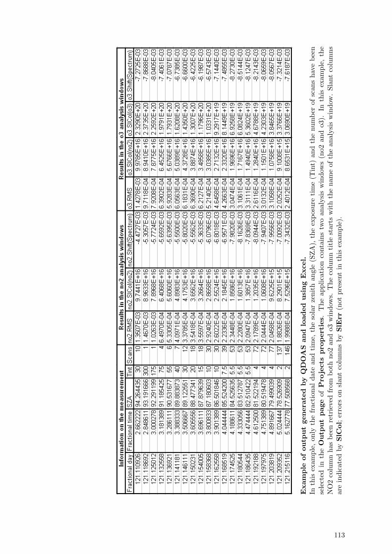
Exam
ple
of
ou
tpu
tgen
era
ted
by
QD
OA
San
dlo
ad
ed
usi
ng
Excel.
Inth
isex
amp
le,
only
the
frac
tion
ald
ate
and
tim
e,th
eso
lar
zen
ith
angl
e(S
ZA
),th
eex
pos
ure
tim
e(T
int)
and
the
nu
mb
erof
scan
sh
ave
bee
nse
lect
edin
the
Ou
tpu
tp
age
ofP
roje
cts
pro
pert
ies.
Th
eap
pli
cati
onco
nta
ins
two
anal
ysi
sw
ind
ows
(no2
an
do3).
Inth
isex
am
ple
,th
eN
O2
colu
mn
has
bee
nre
trie
ved
from
bot
hn
o2an
do3
win
dow
s.T
he
colu
mn
titl
est
arts
wit
hth
en
ame
ofth
ean
aly
sis
win
dow
.Sla
nt
colu
mn
sare
ind
icat
edby
SlC
ol;
erro
rson
slan
tco
lum
ns
by
SlE
rr(n
otp
rese
nt
inth
isex
amp
le).
113

Exam
ple
of
ou
tpu
tfi
legen
era
ted
by
QD
OA
San
dlo
ad
ed
usi
ng
Excel.
Th
isex
am
ple
has
bee
nge
ner
ated
from
asa
tell
ite
app
lica
tion
(GO
ME
-2).
Res
ult
sof
the
fit
are
not
show
nh
ere.
For
sate
llit
em
easu
rem
ents
,th
eacc
ura
cyof
the
mea
sure
men
tti
me
isim
por
tant.
Th
efo
rmat
YY
YY
MM
DD
hh
mm
ss(y
ear,
mon
th,
day
,h
our,
min
ute
,se
con
dacc
ola
ted
;m
illi
seco
nd
sin
the
frac
tion
alp
art)
isu
sual
lyp
refe
rred
toth
efr
acti
onal
dat
ean
dti
me.
Geo
loca
tion
coor
din
ates
are
give
nat
the
fou
rco
rner
san
dat
the
centr
eof
the
pix
el.
Angl
essu
chas
the
sola
rze
nit
han
gles
are
given
atth
eb
egin
nin
g,th
em
idd
lean
dth
een
dof
the
mea
sure
men
t.
114
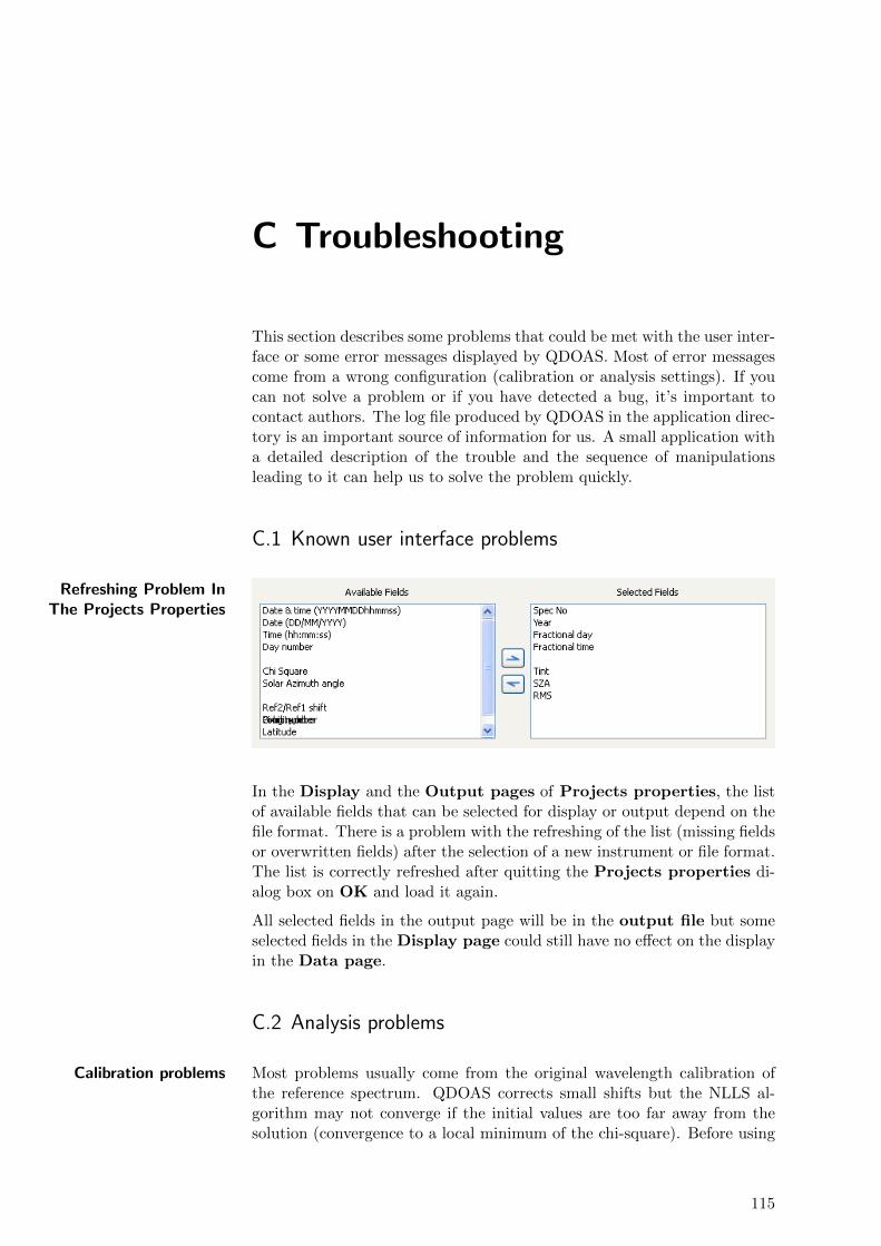
C Troubleshooting
This section describes some problems that could be met with the user inter-face or some error messages displayed by QDOAS. Most of error messagescome from a wrong configuration (calibration or analysis settings). If youcan not solve a problem or if you have detected a bug, it’s important tocontact authors. The log file produced by QDOAS in the application direc-tory is an important source of information for us. A small application witha detailed description of the trouble and the sequence of manipulationsleading to it can help us to solve the problem quickly.
C.1 Known user interface problems
Refreshing Problem InThe Projects Properties
In the Display and the Output pages of Projects properties, the listof available fields that can be selected for display or output depend on thefile format. There is a problem with the refreshing of the list (missing fieldsor overwritten fields) after the selection of a new instrument or file format.The list is correctly refreshed after quitting the Projects properties di-alog box on OK and load it again.
All selected fields in the output page will be in the output file but someselected fields in the Display page could still have no effect on the displayin the Data page.
C.2 Analysis problems
Calibration problems Most problems usually come from the original wavelength calibration ofthe reference spectrum. QDOAS corrects small shifts but the NLLS al-gorithm may not converge if the initial values are too far away from thesolution (convergence to a local minimum of the chi-square). Before using
115
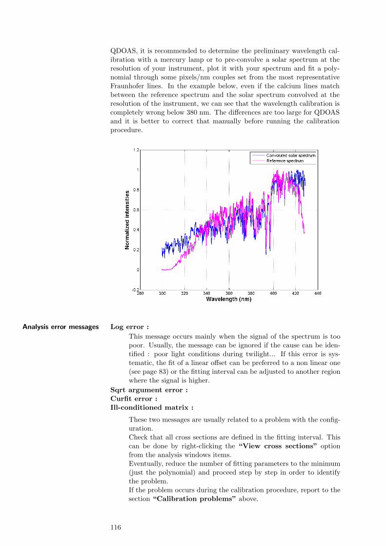
QDOAS, it is recommended to determine the preliminary wavelength cal-ibration with a mercury lamp or to pre-convolve a solar spectrum at theresolution of your instrument, plot it with your spectrum and fit a poly-nomial through some pixels/nm couples set from the most representativeFraunhofer lines. In the example below, even if the calcium lines matchbetween the reference spectrum and the solar spectrum convolved at theresolution of the instrument, we can see that the wavelength calibration iscompletely wrong below 380 nm. The differences are too large for QDOASand it is better to correct that manually before running the calibrationprocedure.
Analysis error messages Log error :
This message occurs mainly when the signal of the spectrum is toopoor. Usually, the message can be ignored if the cause can be iden-tified : poor light conditions during twilight... If this error is sys-tematic, the fit of a linear offset can be preferred to a non linear one(see page 83) or the fitting interval can be adjusted to another regionwhere the signal is higher.
Sqrt argument error :Curfit error :Ill-conditioned matrix :
These two messages are usually related to a problem with the config-uration.Check that all cross sections are defined in the fitting interval. Thiscan be done by right-clicking the “View cross sections” optionfrom the analysis windows items.Eventually, reduce the number of fitting parameters to the minimum(just the polynomial) and proceed step by step in order to identifythe problem.If the problem occurs during the calibration procedure, report to thesection “Calibration problems” above.
116
Allocation error during the Kurucz procedure :
The degree of the polynomial fitting the continuous part of spectrumhas not been defined in the “Linear parameters page” (see Cal-ibration page of Projects Properties, page 67).
spline interpolation requests increasing absissae (...) :
The problem can come from a bad input file (preliminary wavelengthcalibration in the “Instrumental page” of Projects properties,cross section, reference spectrum) or the wavelength calibration pro-cedure doesn’t succeed to correct the preliminary wavelength calibra-tion (report to the section “Calibration problems” above).
Number of degree of freedom <= 0... :
Too many parameters are fitted w.r.t. the size of the fitting intervalor the settings of the filter are not suitable. Reduce the number ofparameters to fit, increase the fitting interval or adjust the size ofthe filter. Check also the calibration settings (Calibration page ofProjects Properties).
Cross section file is empty or not large enough :
Check that all cross sections are defined in the fitting interval. Thiscan be done by right-clicking the “View cross sections” optionfrom the analysis windows items. Do not also forget the cross sectionsand the solar spectrum defined in the Calibration page of ProjectsProperties.
117

Glossary
AMF Air Mass Factor
ASCII American Standard Code for Information Interchange
BEAT Basic Envisat Atmospheric Toolbox
BIRA-IASB Royal Belgian Institute for Space Aeronomy
Cic Colour Index
CINDI Cabauw Intercomparison Campaign of Nitrogen Dioxide measuringInstruments
CODA Common Data Access Toolbox
DISORT Discrete Ordinates Radiative Transfer program
DOAS Differential Optical Absorption Spectroscopy
DOASIS DOAS Intelligent System
ENVISAT Environmental Satellite
ERS European Remote Sensing Satellite
FFT Fast Fourier Transform
FWHM Full Width at Half Maximum
GDP Gome Data Processor
GOME Global Ozone Monitoring Experiment
GPL General Public License
GUI Graphical User Interface
HDF Hierarchical Data Format
HDF-EOS Hierarchical Data Format - Earth Observing System
HTML Hypertext Markup Language
JPG Graphics file format developed by the Joint Photographics ExpertGroup
LIDORT Linearized Discrete Ordinate Radiative Transfer Program
M-L Marquardt-Levenberg
119

MAXDOAS Multi-Axis DOAS
METOP Meteorological Operational satellite
NDACC Network for the Detection of Atmospheric Composition Change
NLLS Non-Linear Least Squares
OHP Observatoire de Haute Provence, France
OMI Ozone Monitoring Instrument
PDS Payload Data Segment (SCIAMACHY)
PNG Portable Network Graphics format
RMS Root Mean Square
RRS Rotational Raman Scattering
S[&]T Science and Technology http://www.stcorp.nl
SAOZ Systeme d’Analyse par Observation Zenithale
SCD Slant Column Density
SCIAMACHY Scanning Imaging Absorption spectrometer for AtmosphericCartography
SFP Slit Function Parameter
SZA Solar Zenith Angle
VCD Vertical Column Density
XML Extensible Markup Language
120
Bibliography
[1] Aliwell, S., Van Roozendael, M., Johnston, P., Richter, A., Wagner, T.,Arlander, D. W., Burrows, J. P., Fish, D. J., Jones, R. L., Tørnkvist,K. K., Lambert, J.-C., Pfeilsticker, K., and Pundt, I. (2002). Analysisfor BrO in zenith-sky spectra: An intercomparison exercise for analysisimprovement. Journal of Geophysical Research, 107(D14).
[2] Beirle, S., Lampel, J., Lerot, C., Sihler, H., and Wagner, T. (2017). Pa-rameterizing the instrumental spectral response function and its changesby a super-gaussian and its derivatives. Atmos. Meas. Tech., 10(10):581–598.
[3] Bevington, P. R. (1969). Data reduction and error analysis for thephysical sciences. McGraw-Hill.
[4] Boersma, K. F., Eskes, H. J., and Brinksma, E. J. (2004). Error anal-ysis for tropospheric NO2 retrieval from space. Journal of GeophysicalResearch, 109(D4).
[5] Bogumil, K., Orphal, J., Homann, T., Voigt, S., Spietz, P., Fleis-chmann, O. C., Vogel, A., Hartmann, M., Kromminga, H., Bovensmann,H., and et al. (2003). Measurements of molecular absorption spectrawith the SCIAMACHY pre-flight model: instrument characterizationand reference data for atmospheric remote-sensing in the 230–2380 nmregion. Journal of Photochemistry and Photobiology A Chemistry, 157(2-3):167–184.
[6] Burrows, J. P., Richter, A., Dehn, A., Deters, B., Himmelmann, S.,Voigt, S., and Orphal, J. (1999). Atmospheric remote-sensing referencedata from GOME-2. temperature-dependent absorption cross sectionsof O3 in the 231–794nm range. Journal of Quantitative Spectroscopy andRadiative Transfer, 61(4):509–517.
[7] Chance, K. (1998). Analysis of BrO measurements from theglobal ozone monitoring experiment. Geophysical Research Letters,25(17):3335–3338.
[8] Chance, K. and Kurucz, R. L. (2010). An improved high-resolutionsolar reference spectrum for earth’s atmosphere measurements in the ul-traviolet, visible, and near infrared. Journal of Quantitative Spectroscopyand Radiative Transfer, 111(9):1289–1295.
[9] Chance, K. V. and Spurr, R. J. (1997). Ring effect studies: Rayleighscattering, including molecular parameters for rotational Raman scat-tering, and the Fraunhofer spectrum. Applied optics, 36(21):5224–5230.
121
[10] Gottwald, M., Bovensmann, H., Lichtenberg, G., Noel, S., von Bargen,A., Slijkhuis, S., Piters, A., Hoogeveen, R., von Savigny, C., Buchwitz,M., Kokhanovsky, A., Richter, A., Rozanov, A., Holzer-Popp, T., Bram-stedt, K., Lambert, J.-C., Skupin, J., Wittrock, F., Schrijver, H., andBurrows, J. (2006). SCIAMACHY, Monitoring the Changing Earth’sAtmosphere. DLR.
[11] Grainger, J. F. and Ring, J. (1962). Anomalous fraunhofer line profiles.Nature, 193(4817).
[12] Hermans, C., Vandaele, A. C., Carleer, M., Fally, S., Colin, R., Jenou-vrier, A., Coquart, B., and Merienne, M. F. (1999). Absorption cross-sections of atmospheric constituents: NO2, O2, and H2O. Environmentalscience and pollution research international, 6(3):151–158.
[13] Kaiser, J. F. and Reed, W. A. (1977). Data smoothing using low-passdigital filters. Review of Scientific Instruments, 48(11):1447–1457.
[14] Kuntz, M. (1997). A new implementation of the humlicek algorithmfor the calculation of the voigt profile function. Journal of QuantitativeSpectroscopy and Radiative Transfer, 57(6):819–824.
[15] Kurucz, R. L. (1995). The solar spectrum: Atlases and line identifica-tions. In Sauval, A. J., Blomme, R., and Grevesse, N., editors, Laboratoryand Astronomical High Resolution Spectra, volume 81 of AstronomicalSociety of the Pacific Conference Series, page 17.
[16] Marquardt, D. W. (1963). An Algorithm for Least-Squares Estima-tion of Nonlinear Parameters. Journal of the Society for Industrial andApplied Mathematics, 11(2):431–441.
[17] OMI IODS (2009). GDPS Input/Output Data Specification (IODS)Volume 2: Level 1B Output products and Metadata. Dutch Space,8 edition. http://disc.sci.gsfc.nasa.gov/Aura/data-holdings/
OMI/documents/v003/RD01_SD467_IODS_Vol_2_issue8.pdf.
[18] Platt, U. (1994). Air Monitoring by Spectroscopic Techniques, volume127 of Chemical Analysis Series, chapter 2, pages 27–84. Wiley.
[19] Platt, U. and Stutz, J. (2008). Differential Optical Absorption Spec-troscopy: Principles and Applications. Physics of Earth and Space En-vironments. Springer, Berlin.
[20] Press, W. H., Flannery, B. P., Teukolsky, S. A., and Vetterling, W. T.(1992). Numerical Recipes in C: The Art of Scientific Computing, SecondEdition. Cambridge University Press, 2 edition.
[21] Press, W. H., Teukolsky, S. A., Vetterling, W. T., and Flannery, B. P.(2007). Numerical Recipes Source Code CD-ROM 3rd Edition: The Artof Scientific Computing. Cambridge University Press, 3 edition.
[22] Roscoe, H. K., Van Roozendael, M., Fayt, C., du Piesanie, A., Abuhas-san, N., Adams, C., Akrami, M., Cede, A., Chong, J., Clemer, K.,Friess, U., Gil Ojeda, M., Goutail, F., Graves, R., Griesfeller, A., Gross-mann, K., Hemerijckx, G., Hendrick, F., Herman, J., Hermans, C., Irie,H., Johnston, P. V., Kanaya, Y., Kreher, K., Leigh, R., Merlaud, A.,
122

Mount, G. H., Navarro, M., Oetjen, H., Pazmino, A., Perez-Camacho,M., Peters, E., Pinardi, G., Puentedura, O., Richter, A., Schonhardt,A., Shaiganfar, R., Spinei, E., Strong, K., Takashima, H., Vlemmix,T., Vrekoussis, M., Wagner, T., Wittrock, F., Yela, M., Yilmaz, S.,Boersma, K. F., Hains, J., Kroon, M., and Piters, A. (2010). Intercom-parison of slant column measurements of NO2 and O4 by MAX-DOASand zenith-sky UV and visible spectrometers. Atmos. Meas. Tech. Dis-cuss., 3(4):3383–3423.
[23] Solomon, S., Schmeltekopf, A. L., and Sanders, R. W. (1987). Onthe interpretation of zenith sky absorption measurements. Journal ofGeophysical Research, 92(D7):8311–8319.
[24] Stutz, J. and Platt, U. (1996). Numerical analysis and estimation ofthe statistical error of differential optical absorption spectroscopy mea-surements with least-squares methods. Applied Optics, 35:6041–6053.
[25] Theys, N., Van Roozendael, M., Hendrick, F., Fayt, C., Hermans, C.,Baray, J., Goutail, F., and Pommereau, J. (2007). Retrieval of strato-spheric and tropospheric BrO columns from multi-axis DOAS mea-surements at reunion island (21oS, 56oE). Atmospheric Chemistry andPhysics, pages 4733–4749.
[26] Van Roozendael, M., Soebijanta, V., Fayt, C., and Lambert, J. (2002).Investigation of DOAS issues affecting the accuracy of the GDP version3.0 total ozone product. In ERS-2 GOME GDP 3.0 Implementationand Delta Validation.
[27] Vandaele, A. C., Hermans, C., Simon, P. C., Van Roozendael, M.,Guilmot, J. M., Carleer, M., and Colin, R. (1996). Fourier transformmeasurement of NO2 absorption cross-section in the visible range atroom temperature. Journal of Atmospheric Chemistry, 25:289–305.
[28] Wagner, T. (1999). Satellite Observations of Atmospheric HalogenOxides. PhD thesis, Universitat Heidelberg.
[29] Wagner, T., Beirle, S., and Deutschmann, T. (2009a). Three-dimensional simulation of the Ring effect in observations of scatteredsun light using Monte Carlo radiative transfer models. Atmos. Meas.Tech., 2(1):113–124.
[30] Wagner, T., Beirle, S., Deutschmann, T., and Penning De Vries, M.(2010). A sensitivity analysis of Ring effect to aerosol properties andcomparison to satellite observations. Atmos. Meas. Tech., 3(6):1723–1751.
[31] Wagner, T., Deutschmann, T., and Platt, U. (2009b). Determinationof aerosol properties from MAX-DOAS observations of the Ring effect.Atmos. Meas. Tech., 2(2):495–512.
123