UPPSALA UNIVERSITYDepartment of Information Technology

Pulse-modulated Feedback inMathematical Modeling andEstimation of Endocrine Systems

PER MATTSSON

IT Licentiate theses2014-006

Pulse-modulated Feedback in

Mathematical Modeling andEstimation of Endocrine Systems

Per Mattssonper.mattsson@it.uu.se

September 2014

Division of System and ControlDepartment of Information Technology

Uppsala UniversityBox 337

SE-751 05 UppsalaSweden

http://www.it.uu.se/

Dissertation for the degree of Licentiate of Philosophy in Electrical Engineering with

Specialization in Automatic Control

c© Per Mattsson 2014

ISSN 1404-5117

Printed by the Department of Information Technology, Uppsala University, Sweden

Abstract

This licentiate thesis is concerned with mathematical modeling and esti-mation of endocrine systems. Hence it also deals with systems biology, aresearch field that has gained a lot of interest during the last decades. Sys-tems biology can be seen as the systematic study of complex interactions inbiological systems, mainly by methods from dynamical systems theory.

The thesis addresses the testosterone (Te) regulation in the human male,but the techniques developed here might be useful for studying other en-docrine loops and axes as well.

In the endocrine system of Te regulation, an essential role is also playedby the luteinizing hormone (LH) and gonadotropin-releasing hormone (GnRH).Together, these hormones form a closed-loop dynamical system with a pulse-modulated feedback implemented by the pulsatile secretion of GnRH. Math-ematical models portraying the interactions between the hormones are in-strumental in obtaining insights into the dynamical phenomena arising inthe endocrine systems. Such models can also serve as a formal basis fordeveloping strategies of medical interventions.

The contribution of the thesis can be divided into two parts: one coveringmathematical models of Te regulation and another suggesting and validatingidentification techniques for those models.

Regarding mathematical modeling, previously suggested and biologicallymotivated models of pulsatile Te regulation have been extended to includetime delays and nonlinear dynamics, for the purpose of better agreementwith clinical data.

In the identification part of the thesis, methods for estimating the un-known parameters in the pulsatile models suggested in the modeling parthave been proposed. This part of the thesis also covers model-based es-timation of signals that cannot be measured in a non-invasive way. Theperformance of the developed identification methods is illustrated on simu-lated and clinical data.

2

Acknowledgment

I would like to thank my supervisor Professor Alexander Medvedev for hissupport, guidance, and for sharing his knowledge and expertise through-out this work. A special thank also goes to Professor Alexander Churilovfor many interesting and fruitful discussions. And a big thank to all mycolleagues at SysCon for providing such a joyful working environment.

I would also like to thank the European Research Council for fundingthe work done in this thesis under the Advanced Grant 247035 (SysTEAM).

Last but not least I would like to thank my family, without you I wouldnot be the one I am today.

3

4

Contents

1 Introduction 71.1 Contribution and publications . . . . . . . . . . . . . . . . . . 71.2 Outline of thesis . . . . . . . . . . . . . . . . . . . . . . . . . 8

2 The Endocrine System 92.1 Testosterone regulation . . . . . . . . . . . . . . . . . . . . . 9

3 Pulse-modulated feedback 133.1 Pulse-modulated feedback control of linear systems . . . . . . 143.2 Time delays . . . . . . . . . . . . . . . . . . . . . . . . . . . . 16

3.2.1 Finite-dimensional approximations . . . . . . . . . . . 16

4 Modeling of endocrine systems 214.1 The Smith Model of Testosterone Regulation . . . . . . . . . 214.2 Convolution models . . . . . . . . . . . . . . . . . . . . . . . 234.3 The Pulse-Modulated Smith Model . . . . . . . . . . . . . . . 24

4.3.1 Extensions of the pulse-modulated Smith model . . . 25

Bibliography 27

5

6

Chapter 1

Introduction

The research field of systems biology has gained a lot of interest during thelast decades. Systems biology can be seen as the systematic study of com-plex interactions in biological systems, mainly by methods from dynamicalsystems theory.

One of the reasons for the success of system biology is that any living or-ganism is a complex system with numerous interacting subsystems, utilizingmultiple feedback loops. Thus it fits well into the framework of dynamicalsystems theory.

There are mainly two different purposes for studying biological systemsusing mathematical modelling. First it can give new insights into the biolog-ical system at hand, and furthermore, these insights together with mathe-matical tools from e.g. control theory can be used to construct new strategiesfor medical interventions.

The notions of feedback and feedforward are particularly important inthe studies of the endocrine system that uses chemical signaling substancescalled hormones for communication between cells and organs. The humanendocrine system affects all aspects of the physiological and behavioral activ-ities. It is thus of interest to obtain a deeper understanding of the dynamicsin the endocrine system, and how failures in this system can be recuperatedor circumvented.

1.1 Contribution and publications

This thesis mainly deals with the testosterone (Te) regulation in the humanmale, but techniques developed here might be useful for studying otherparts of the endocrine system too. The contribution of the thesis can bedivided into two parts: one covering mathematical models of Te regulationand another suggesting and validating identification techniques for those

7

models. Regarding modeling, existing models of testosterone regulation havebeen extended with time delays and nonlinear dynamics, with the purposeof achieving better fit to clinical data. The identification part treats theestimation of unknown model parameters, and estimation of signals thatcannot be measured in a non-invasive way.

The thesis comprises the following papers:

Paper I P. Mattsson, and A. Medvedev , “Estimation of input impulsesby means of continuous finite memory observers”, American ControlConference (ACC), Montreal, Canada, 2012.

Paper II P. Mattsson, and A. Medvedev, “State Estimation in LinearTime-Invariant Systems With Unknown Impulsive Inputs”, EuropeanControl Conference (ECC), Zurich, Switzerland, 2013.

Paper III A. Churilov, A. Medvedev, and P. Mattsson, “Periodical Solu-tions in a Pulse-Modulated Model of Endocrine Regulation With Time-Delay”, IEEE Transactions on Automatic Control, 59(3) : 728–733,2014.

Paper IV P. Mattsson, and A. Medvedev, “Modeling of Testosterone Reg-ulation by Pulse-modulated Feedback: An Experimental Data Study”,International Symposium on Computational Models for Life Sciences,Sydney, Australia, 2013.

Additional material pertaining to the topic of this thesis is presented in thefollowing publications that are not part of this manuscript:

• A. Churilov, A. Medvedev, and P. Mattsson, “Analysis of a pulse-modulated model of endocrine regulation with time-delay”, IEEE Con-ference on Decision and Control (CDC), Maui, USA, 2012.

• A. Churilov, A. Medvedev and P. Mattsson, “On Finite-dimensionalReducibility of Time-delay Systems under Pulse-modulated Feedback”,IEEE Conference on Decision and Control (CDC), Florence, Italy,2013.

1.2 Outline of thesis

This thesis is divided into three major blocks. The first block provides anintroduction to endocrine systems in general and testosterone regulation inparticular. The second block gives some theoretical background to pulse-modulated systems that are extensively utilized in the appended papers ofthe thesis. Finally, in the third block, the principles of pulse-modulation areapplied to modelling of testosterone regulation in the human male.

8

Chapter 2

The Endocrine System

The endocrine system consists of all the cells, glands, and tissues that pro-duce hormones inside the body. Hormones are biochemicals that are syn-thesized by the glands, and secreted into the bloodstream. In this way hor-mones act as chemical messengers that transfer information between cells,and thus, also organs.

The endocrine system also communicates with the nervous systems throughthe hypothalamus in the brain. The nervous system sends information tohypothalamus about changes in the body, and regulates the production ofhormones in the pituitary gland. In this way both the endocrine and nervoussystem can use feedback to control physiological and behavioral processesof the organism. Due to feedback loops, the secretion of a hormone is stim-ulated (or inhibited) by other hormone or hormones. That is, the secretionrate of one hormone depends on the concentration (or concentration changerate) of other hormones. After hormone molecules have been synthesizedand released into the bloodstream, they will maintain a biologically activestate for a while, and then, like all organic molecules, they will degrade. Theprocess of degradation is referred to as elimination or clearing of hormones.

The above description of the endocrine system, with secretion and elim-ination rates, as well as feedback loops, indicates that it can be seen as adynamical system. This thus suggests that the theory of dynamical systemscould be useful for modelling and analysis of endocrine systems.

2.1 Testosterone regulation

The endocrine system can be divided into several subsystems that are re-sponsible for different physiological functions. In mammals, one importantobjective of the endocrine system is to control the reproductive system. Inthe human male, this is primarily done through the regulation of the male

9

GnRH

LH

Te

(+)

(+)

(-)

Hypothalamus

Pituitary

Testis

Figure 2.1: Schematic diagram of the male hypothalamic-pituitary-gonadalsystem. Arrows denote feedforward (stimulatory (+)) and feedback (in-hibitory (-)) actions.

sex hormone – testosterone (Te). Testosterone levels are also involved in thegrowth of muscle, bones and fat tissue, among other things.

The testosterone regulation system is schematically depicted in Fig. 2.1.It mainly comprises two other hormones: luteinizing hormone (LH) andgonadotropin-releasing hormone (GnRH). GnRH is a neurohormone releasedin the hypothalamus of the brain. GnRH then stimulates the secretion ofLH by the pituitary gland. LH travels through the bloodstream to the testeswhere it stimulates the secretion of Te. Finally, the feedback loop is closedby Te inhibiting the secretion of both LH and GnRH [1]. However, theinhibition of LH has a relatively small effect on the closed-loop system, andis therefore not considered in this thesis.

There are several reasons for studying the dynamics of testosterone reg-ulation in the human male. To start with, a pragmatic reason is that it isone of the simplest endocrine subsystems, involving mainly three differenthormones in the axis GnRH-LH-Te. At the same time, the regulation of Teshares many common aspects with regulation in other parts of the endocrinesystems, e.g. those handling cortisol, growth hormone, and insulin. Thus,methods developed for modeling of Te regulation in this thesis can hopefullybe used for other parts of the endocrine system in the future.

Furthermore, Te regulation, being an integral part of the reproductivesystem in the human male, constitutes an interesting research topic on itsown right. Understanding how the Te regulation works would help planningmedical interventions such as testosterone replacement therapy. Accurate

10

mathematical models can then help researchers to get a deeper insights intothe closed-loop dynamics in Te regulation, as well as be an aid in optimizingtherapies.

11

12

Chapter 3

Pulse-modulated feedback

A typical feedback control system is schematically depicted in Fig. 3. Itconsists of a dynamical system S, whose output is desired to follow a certainreference signal. This can be achieved by using a feedback controller C thatuses the reference signal and the system output to compute a suitable inputsignal for S.

The field of control theory started the emerge in the first half of the20th century [2]. Today, feedback control is an integral part of most engi-neered systems. A reason for the success of feedback control is that it cancreate control strategies that perform well even though the components ofthe system perform poorly, e.g. due to wear and tear. This property is ofcourse also desirable when it comes to the functions inside the human body,so it should come as no surprise that evolution has equipped humans withnumerous feedback mechanisms, from the cell level to the level of the com-plete organism. One such system, equipped with multiple feedback loops ofdifferent kinds, is the endocrine system.

In pulse-modulated control, the controller C feeds the system with asignal that consists of a train of pulses fired at discrete time instants. Dueto, among other things, simple realization and low power consumption, thistype of control have been used in areas such as electrical, space, heating andpneumatic engineering [3]. Due the pulsatile nature of neural networks andhormone secretion [4], it has also found it uses in modelling of biomedicalsystems [5].

OutputReference

SCInput

Figure 3.1: Block diagram of a feedback control system

13

3.1 Pulse-modulated feedback control of linear sys-tems

In pulse-modulated feedback, different pulse types can be used, e.g. rect-angular ones. However, here only impulses described by the Dirac deltafunction δ(·) are considered. Each impulse in the sequence has a correspond-ing impulse time tk and impulse weight λk. Arbitrary signal shapes can becreated by adding a (known) filter whose impulse response implements thedesired pulse shape.

If the plant S is a linear system with the state vector x and the outputy, the pulse-modulated system can be formulated as

x(t) = Ax(t) +Bξ(t), y(t) = Cx(t), (3.1)

where

ξ(t) =

∞∑k=0

λkδ(t− tk). (3.2)

Note that the impulse at time tk makes the state vector jump with theamplitude λk. Thus system (3.1)-(3.2) can equivalently be formulated as ahybrid system, where the state vector evolves continuously according to alinear equation, but jumps at discrete times tk:

x(t) = Ax(t), if t �= tk (3.3)

x(t+k ) = x(t−k ) + λkB, if t = tk. (3.4)

The time between the impulses, sometimes called the clock interval, will bedenoted by Tk = tk+1 − tk.

A pulse-modulated system can be controlled in several different ways. Inamplitude modulation, the clock intervals Tk are predetermined, e.g. haveuniform length, and the amplitude λk of each pulse is determined by thecontrol mechanism. In frequency modulation, on the other hand, the lengthof each clock interval Tk is determined by the controller, while the amplitudesare predetermined.

In this thesis, amplitude-frequency pulse-modulation is used. Here thegoal for the controller is to choose both the impulse times tk and the impulseweights λk in such a way that a desired behaviour of the plant is achieved.In the literature, a distinction is typically made between two types of pulse-modulated control. A first possibility is that the length of the clock intervalTk and the corresponding amplitude λk are determined directly by the out-put in the beginning of each interval. That is,

tk+1 = tk + Tk, Tk = Φ(y(t−k )), λk = F (y(t−k )), (3.5)

14

for some static functions Φ(·) and F (·). This type of modulation is refereedto as modulation of the first kind.

However, other types of modulation are possible. For example, the nextclock interval Tk could be determined as the minimal positive root of theequation

Tk = Φ(σ(tk)), (3.6)

where σ(tk) is a function that depends on the output in the interval [tk−1, tk].In this way, all information from the output can be used to determine thecontrol signal. This is called modulation of the second kind.

In the modelling part of this thesis, only modulation of the first kind isconsidered. One reason for this is that it simplifies the analysis of the dy-namical model. Also, only autonomous closed-loop systems are considered,and in this case the behaviour of the controller in between impulse times canin principle be encoded into the modulation functions Φ(·) and F (·). Hence,concentrating on modulation of the first kind is not a severe restriction inthis case.

Assuming that Φ(·) and F (·) are strictly positive and bounded, the modeldescribed by (3.3)-(3.5) is a self-sustained oscillating system. Thus it isof interest to study its periodic solutions. In [6] stability and oscillationsof pulse-modulated systems are investigated. Periodical solutions of thespecific model given by (3.3)-(3.5) are analyzed in [5] .

From the equations of the model, it is straightforward to derive a mapdescribing how the state vector x propagates from the impulse time tk totk+1. That is,

x(t−k+1) = Q(x(t−k )), (3.7)

whereQ(x) = eAΦ(Cx)(x+ F (Cx)B). (3.8)

By means of the above equation, different types of periodical solutions ofsystem (3.1),(3.5) can be studied. For example, if xo is a fixed point of (3.7),i.e.,

Q(xo) = xo (3.9)

then a solution to (3.3)-(3.5) with the initial condition x(t−0 ) = xo will beperiodic with one impulse in each period. Such a solution is called a 1-cycle.In [5], it is shown that a 1-cycle is locally stable if the matrix

Q′(xo) = eAΦ(Cxo)[I + F ′(Cxo)BC] + Φ′(Cxo)AQ(xo)C (3.10)

is Schur stable, i.e. if the Jacobian Q′(xo) has all eigenvalues inside theunit circle. There are also similar condition for higher order cycles, see [5].Bifurcation analysis of the model considered here is carried out in [7], whereit is demonstrated that the model can exhibit stable periodic cycles of highmultiplicity as well as deterministic chaos.

15

3.2 Time delays

In many applications, time delays arising between different parts of the stud-ied system play a prominent role. In, for example testosterone regulation, ittakes time for LH to travel from the pituitary to the testes. It also takes timefor the testes to produce testosterone in response to the LH stimulation.

A time delay can be introduced into the pulse-modulated model in Sec-tion 3.1 as

x(t) = A0x(t) +A1x(t− τ) +Bξ(t), y(t) = Cx(t) (3.11)

where τ ≥ 0. The same type of questions as asked about periodical solutionsand stability of the mathematical model in Section 3.1, can also be askedabout the time-delay models. Some analytical results regarding (3.11), sim-ilar to the ones in [5] for the time delay-free case, are presented in Paper III.

3.2.1 Finite-dimensional approximations

As can be seen in Paper III, the analysis of the system becomes much moreinvolved when time delays are included in the model. For that reason, itmight be suitable to see whether a finite-dimensional system can approxi-mately capture the dynamics of (3.11).

When a linear time-invariant system is augmented with a time-delay oflength τ , the transfer function will contain the exponential factor e−τs. Acommon way to perform finite-dimensional approximation of the time-delaysystem is to replace e−τs with a rational function that approximates theexponential.

Here two approximations of e−τs will be considered, namely the Padeapproximation [8] and the Laguerre approximation [9]. The Pade approxi-mation is arguably the most common way to approximate a time-delay in alinear system. The Laguerre functions have previously been used to estimatetime delays from impulse responses in linear systems [10].

For the time-delayed pulse-modulated system, the transfer function ofthe linear part (3.11) is given by

G(s) = C(sI −A0 −A1e

−τs)−1

B. (3.12)

Replacing e−τs with a rational function of order k, gives a rational transferfunction G(s) that approximates G(s). Now let A, B and C be the systemmatrices in a state space realization of G(s) and let xe(t) be the state vector.Then a state-space approximation of (3.12) is

xe(t) = Axe(t) + Bξ(t), y(t) = Cxe(t). (3.13)

16

Note that this model is in the same form as the delay-free case discussedin Section 3.1. Hence, the properties of the approximative system can bestudied using the same tools as before. The question is now, does thisapproximation capture the dynamics of the original model well? There areseveral ways to answer this. For example, assume that the original systemhas a stable 1-cycle, will the approximative system have a stable 1-cycle ofthe same period? Further, will the output y(t) of the approximative system,behave in the same way as the output y(t) of the original system?

Assume the following numerical values in (3.11)

A0 =

⎡⎣−0.4 0 0

1 −0.01 00 0 −0.046

⎤⎦ , A1 =

⎡⎣0 0 00 0 00 1 0

⎤⎦ , (3.14)

B =

⎡⎣100

⎤⎦ , C =

[0 0 1

](3.15)

and choose the modulation functions in (3.5) as

Φ(y) = 50 + 150(y/r)2

1 + (y/r)2, F (y) = 1.5 +

5

1 + (x/r)2, (3.16)

where r = 50 and the time delay is τ = 40. Then (3.11) will have a stable1-cycle with a period T0 = 157.61. Fig. 3.2 shows how the period T0 ofthe 1-cycle in the approximative system G(s) behaves for different ordersof approximation, both when the Pade and Laguerre functions are used. Itcan be seen that the Pade approximation converges towards the true periodfor low orders of approximation. The Laguerre approximation on the otherhand does not accurately capture the period well even when the order ofapproximation is increased to 20.

Fig. 3.3 depicts the output of the original time-delay system in a 1-cycle,as well as the output of the finite-dimensional approximation for differentorders of Pade and Laguerre approximations. It can be seen that the Padeapproximation has close agreement in signal form already for low approx-imation orders. For the Laguerre approximation, it can be seen that thesignal form gets closer to the true output when the approximation order isincreased, but since it does not capture the period of the 1-cycle very well, itwill diverge from the true signal after a few periods even for approximationorder 20.

These simulations indicate that even though Laguerre functions havebeen useful in identifying the time-delay in an impulse response, the Pade ap-proximation seems to be preferable when a time delay in a pulse-modulated

17

0 5 10 15 200

2

4

6

8

10

12

Approximation order

|T0−

To|

PadeLaguerre

Figure 3.2: The approximation error of a 1-cycles time period for differ-ent orders of the Pade and Laguerre approximations. The original infi-nite dimensional system is given by (3.14)-(3.16), and has a time periodT0 = 157.61. The time period T0 of the approximative system varies withthe approximation order. The poles of the Laguerre functions are set to0.15.

0 50 100 150 200 250 300 350 400 450 50050

100

150

Out

put

0 50 100 150 200 250 300 350 400 450 50050

100

150

Out

put

0 50 100 150 200 250 300 350 400 450 50050

100

150

Out

put

Time, t

Original systemPade approximation

of order 5

Original systemPade approximation

of order 10

Original systemPade approximation

of order 20

0 50 100 150 200 250 300 350 400 450 50050

100

150

200

Out

put

0 50 100 150 200 250 300 350 400 450 50050

100

150

200

Out

put

0 50 100 150 200 250 300 350 400 450 50050

100

150

Out

put

Time, t

Original systemLaguerre approximation

of order 5

Original systemLaguerre approximation

of order 10

Original systemLaguerre approximation

of order 20

Figure 3.3: Output of the original (y(t)) and approximated (y(t)) for ap-proximation orders 5, 10 and 20. In the left figure, the Pade approximationis used, and in the right the Laguerre approximation is used.

18

system is to be approximated. Similar simulations have been carried outwith different sets of parameters, with similar results.

The numerical experiments also indicate that already low-order rationalapproximations of time-delay in systems under pulse-modulated feedbackare instrumental in predicting the closed-loop system behaviour. This raisesa concern about identifiability of the continuous part of the system fromclosed-loop data, since it would be difficult to tell whether the dynamics ofthe system are finite-dimensional or infinite-dimensional. In order to high-light the presence of the time delay, properly injected exogenous excitationcould however be used.

19

20

Chapter 4

Modeling of endocrinesystems

In mathematical modeling of endocrine systems, a number of plausible ap-proaches can be taken. One possibility is to derive a model from the fun-damental principles of biology, biochemistry, and physics. This approachhas been used in e.g. modeling of the glucose-insulin feedback system indiabetes 1 [11], and in simulating the mechanisms of the human menstrualcycle [12].

However, since endocrine systems usually consist of a complex networkof interacting glands and hormones, such models are typically of high di-mension and very cumbersome to develop. The complexity of the resultingmodels also makes it hard to estimate the parameters of the model, as wellas using it to develop therapy strategies.

In order to obtain insights into the principles of biological feedback viamathematical analysis, a modeling approach where only the most essentialcharacteristics and interactions of the system are included appears to be use-ful. Techniques from system identification [13] can then be used to estimatethe parameters of the model in a systematic way, yielding a relatively sim-ple model that yet can accurately describe how the hormone concentrationsvary with time. This is the approach taken here.

4.1 The Smith Model of Testosterone Regulation

As described in Section 2.1, the endocrine system of Te regulation in themale essentially consists of three hormones, namely Te, LH, and GnRH.GnRH is secreted in an episodic and pulsatile manner in the hypothalamusand stimulates the secretion of LH into the blood by the pituitary gland.LH stimulates, in its turn, the secretion of Te in the testes, see Fig. 2.1.

21

0 20 40 60 80 1000

2

4

x 10 20 40 60 80 100

0

10

20

x 2

0 20 40 60 80 1000

5

10

x 3

Time, t

0 20 40 60 80 1000

2

4

x 1

0 20 40 60 80 1005

10

15

x 2

0 20 40 60 80 1003456

x 3

Time, t

Figure 4.1: Solutions to the Smith model with the nonlinear function f asa Hill function. Left, Hill order ρ = 7. Right, Hill order ρ = 10.

For example, in [14], a reductionist approach was taken to develop aqualitative mathematical model describing the male reproductive system.The model, usually called the Smith model, can be expressed by the followingthree ordinary differential equations

R = f(T )−B1(R),

L = G1(R)−B2(L),

T = G2(L)−B3(T ),

(4.1)

where R(t), L(t) and T (t) represent the serum concentration of GnRH,LH, and Te, respectively. The non-negative functions B1, B2, B3 describethe clearing rates of the hormones and G1, G2, f specify the rates of theirsecretion. Instead of portraying all the complex interactions between theconstituting parts of the endocrine system, the Smith model captures onlythe main features to match the mathematical tools available at that time.

Since it is well known that the concentrations of LH and Te do not stay atconstant levels, only self-sustained oscillating solutions are biologically fea-sible behaviors of the autonomous model in (4.1). The dynamical propertiesof (4.1) have been studied analytically to great extent for different choicesof the functions Bi, Gi and f . It is relatively common to approximate Bi

and Gi by linear functions, so that

Bi(x) = bix, bi > 0, i = 1, 2, 3;

Gi(x) = gix, gi > 0, i = 1, 2.(4.2)

In [14], sufficient conditions for (4.1)-(4.2) to have stable periodic solutionsare given.

Fig. 4.1 shows two solutions of (4.1)-(4.2) with f(x) chosen to be a Hillfunction,

f(x) =K

1 + βxp. (4.3)

It can be seen that the solution converges to a stable stationary point when

22

0 2 4 6 8 1040

60

80

100

120

x

f(x)

ρ=4ρ=8

ρ=2

Figure 4.2: The Hill function (4.3) for different values of ρ.

ρ = 7, and that the solution is periodic when ρ = 10 for the chosen parametervalues. In fact, it was shown in [15] that a necessary condition for a periodicsolution is that ρ > 8, for any choices of the linear parameters. In e.g.[16] and [17], it is argued that such a high value of the Hill function order isunrealistic. Indeed, already for ρ ≥ 4 (cf. Fig. 4.1), the Hill function in (4.3)resembles a relay characteristic that lacks a proper biological justification.

To resolve the above issue, several attempts have been made to extendthe Smith model in such a way that the solutions oscillate for a broaderrange of the parameters, mostly by introducing special types of nonlinearfeedback and time delays. Yet, the Smith model of testosterone regulationin the formulation of [16] is proven to be asymptotically stable for any valueof the time delay under a nonlinear feedback in the form of a first-orderHill function, [18]. However, by introducing a non-smooth feedback such aspiece-wise linear (affine) nonlinearities, multiple periodical orbits and chaosarise in the Smith model [19, 20]. Multiple delays in the Smith model undera second-order Hill function feedback are also shown to lead to sustainednonlinear oscillations in some subspaces of the model parameters [21].

4.2 Convolution models

As described in Section 4.1, there are several problems with using the clas-sical (continuous) closed-loop Smith model. For this reason, at present,analysis of hormone dynamics from measured (blood serum) hormone con-centrations usually only considers open-loop dynamics. It is usually assumedthat the concentration of a single hormone satisfies a linear ordinary differ-ential equation of the form

dC(t)

dt= −bC(t) + S(t), (4.4)

23

where C(t) is the time profile of the concentration, S(t) the hormone secre-tion rate, and b is the rate of elimination, see, e.g. [22]. So, if the hormonein question is LH, then C(t) and S(t) correspond respectively to L(t) andG1(R(t)) in the Smith model, while b corresponds to b2.

For (4.4) it holds that

C(t) =

∫ t

0S(τ)E(t− τ)dτ + C(0)E(t) (4.5)

where E(t) is the impulse response of (4.4), and describes the eliminationrate profile of the hormone. A reasonable and often used model for a hor-mone concentration is therefore the convolution given by (4.5). In order tounderstand the properties of the endocrine system better, it is of interest toknow the time profile of the secretion rate S(t), while only the concentra-tion C(t) is measurable. In this case, deconvolution methods can be used toestimate S(t) from C(t) by exploiting (4.4).

However, if there is no a priori information about the secretion profileS(t) or the impulse response E(t), this problem is usually ill-conditioned.Hence, in most cases, some assumptions on the secretion profile are made,resulting in so-called model-based deconvolution. Many algorithms for esti-mation of hormone secretion rates from concentration data exist, e.g. WENDeconvolution [23], WINSTODEC [24], and AutoDecon [25]. In [23], a com-parison of several different deconvolution approaches is presented.

Most deconvolution-based methods capture major pulsatile secretionevents when used on longer time series. However, they tend to neglect the ex-istence of smaller pulses in between major pulses [26]. In [26] some methodsfor circumventing this problem are proposed. Further, the deconvolution-based methods do not take into account the fact the hormones in the en-docrine system are part of a closed-loop system. In order to capture theclosed-loop dynamics model-based observers can be utilized, see e.g. [27].

4.3 The Pulse-Modulated Smith Model

It is well known that GnRH is released episodically by hypothalamic neuronsin modulated secretory bursts [28]. In e.g. [29], a detailed mathematicaldescription of GnRH pulses is presented.

The pulsatile nature of GnRH is not directly reflected by the classicalSmith model in (4.1), where the resulting oscillating temporal profile of theinvolved hormones is due to smooth nonlinearities.

However, for the purpose of capturing the biologically implemented feed-back mechanism, an element implementing pulse-amplitude and pulse-frequency

24

modulation can be used, as explained in [4]. Thus the mathematical frame-work of pulse-modulated feedback, discussed in Section 3.1, is directly ap-plicable.

An extended version of the Smith model, that makes use of pulse-modulationwas introduced in [5].

In order to extend the Smith model with pulse-modulation, let tk, k =0, 1, 2, . . . be the time instances when a GnRH pulse is released in the blood-stream, and let λk represent the size of the pulse number k. Then a pulse-modulated model of testosterone regulation can be written in a state-spaceform with x ∈ R

3, and x1 = R(t), x2(t) = L(t), x3(t) = T (t), as

x(t) =

⎡⎣−b1 0 0

g1 −b2 00 g2 −b3

⎤⎦x(t), if t �= tk (4.6)

x(t+k ) = x(t−k ) + λk

⎡⎣100

⎤⎦ , if t = tk (4.7)

where b1, b2, b3, g1 and g2 are the positive parameters as in (4.2). The firingtimes tk and the impulse weights λk are then given by the recursion

tk+1 = tk + τk, τk = Φ(x3(t)), λk = F (x3(t)), (4.8)

where Φ(·) is a frequency modulation characteristic and F (·) is an amplitudemodulation characteristic.

The model in (4.6)-(4.8) is referred to as the pulse-modulated Smithmodel, and was analyzed in detail in [5]. It constitutes a hybrid systemthat evolves in continuous time according to (4.6), but undergoes instanta-neous jumps in the continuous state vector at discrete points governed by(4.7). Each jump in the state vector corresponds to the secretion of a GnRHimpulse.

By construction, this model will, just as the biological system, alwayshave sustained oscillations. It thus solves the problem with stationary solu-tions in the classical Smith model discussed in Section 4.1. The dynamicsof (4.6)-(4.8) are thoroughly studied and are known to exhibit oscillatingsolutions that are either periodic or chaotic [7].

4.3.1 Extensions of the pulse-modulated Smith model

One of the contributions in this thesis is extensions of the model presented inSection 4.3. The motivation for these extensions is that the model in (4.6)-(4.8) does not reflect some biological properties of the system that manifestthemselves in clinical data.

25

An important property of testosterone regulation, that is not includedin the pulse-modulated feedback model, is that it takes time for LH secretedin the pituitary to travel, through the bloodstream, to the testes where Teis produced. In [30], it is suggested that it takes about 5 minutes for LH totravel from the pituitary to the testes. Furthermore, there is a time delayof about 25 minutes between LH stimulation of the testes and the releaseof Te. Hence it follows that there is a time delay of about 30 minutes fromthe secretion of LH to the secretion of Te, which is not accounted for in(4.6)-(4.8). In order to add such a time delay, methods described in Section3.2 are used in Paper III.

Furthermore, because of the linear approximation in (4.2), nonlinear ef-fects are not considered in the pulse-modulated model presented here. Un-fortunately, clinical data indicate that saturation actually plays an impor-tant role when it comes to LH stimulation of Te secretion. The biologicalreason for such a saturation is that there is a limited amount of Te that canbe produced during any finite time interval, and clinical data demonstratethat the Te secretion rate actually does saturate in some subjects. In PaperIV, a saturating nonlinearity is added to the model, and estimations of theinvolved parameters are carried out.

26

Bibliography

[1] J. D. Veldhuis, “Recent insights into neuroendocrine mechanisms ofaging of the human male hypothalamic-pituitary-gonadal axis,” Journalof Andrology, vol. 20, no. 1, pp. 1–18, 1999.

[2] K. J. Astrom and P. Kumar, “Control: a perspective,” Automatica,2013.

[3] A. K. Gelig and A. N. Churilov, “Frequency methods in the theoryof pulse-modulated control systems,” Automation and Remote Control,vol. 67, no. 11, pp. 1752–1767, 2006.

[4] J. Walker, J. Terry, K. Tsaneva-Atanasova, S. Armstrong, C. McAr-dle, and S. Lightman, “Encoding and decoding mechanisms of pulsatilehormone secretion,” Journal of Neuroendocrinology, vol. 22, pp. 1226–1238, 2009.

[5] A. Churilov, A. Medvedev, and A. Shepeljavyi, “Mathematical modelof non-basal testosterone regulation in the male by pulse modulatedfeedback,” Automatica, vol. 45, no. 1, pp. 78–85, 2009.

[6] A. K. Gelig and A. N. Churilov, Stability and Oscillations of NonlinearPulse-Modulated Systems. Boston: Birkhauser, 1998.

[7] Z. T. Zhusubaliyev, A. N. Churilov, and A. Medvedev, “Bifurcationphenomena in an impulsive model of non-basal testosterone regulation,”Chaos: An Interdisciplinary Journal of Nonlinear Science, vol. 22,no. 1, 2012.

[8] J. Lam, “Convergence of a class of Pade approximations for delay sys-tems,” International Journal of Control, vol. 52, no. 4, pp. 989–1008,1990.

[9] P. Makila, “Laguerre series approximation of infinite dimensional sys-tems,” Automatica, vol. 26, no. 6, pp. 985 – 995, 1990.

27

[10] E. Hidayat and A. Medvedev, “Laguerre domain identification of con-tinuous linear time-delay systems from impulse response data,” Auto-matica, vol. 48, no. 11, pp. 2902 – 2907, 2012.

[11] B. P. Kovatchev, M. Breton, C. Dalla Man, and C. Cobelli, “In silicopreclinical trials: A proof of concept in closed-loop control of type 1diabetes,” Journal of Diabetes Science and Technology, vol. 3, no. 1,pp. 44–55, January 2009.

[12] N. Rasgon, L. Pumphrey, P. Prolo, S. Elman, A. Negrao, J. Licinio,and A. Garfinkel, “Emergent oscillations in mathematical model of thehuman menstrual cycle,” CNS Spectrums, vol. 8, no. 11, pp. 805–814,2003.

[13] T. Soderstrom and P. Stoica, System Identification. Upper SaddleRiver, NJ, USA: Prentice-Hall, Inc., 1988.

[14] W. R. Smith, “Hypothalamic regulation of pituitary secretion ofluteinizing hormone. II. feedback control of gonadotropin secretion,”Bulletin of Mathematical Biology, vol. 42, no. 1, pp. 57 – 78, 1980.

[15] L. S. Farhy, “Modeling of oscillations in endocrine networks with feed-back,” in Numerical Computer Methods, Part E, ser. Methods in En-zymology, M. L. Johnson and L. Brand, Eds. Academic Press, 2004,vol. 384, pp. 54–81.

[16] J.D. Murray, Mathematical Biology, I: An Introduction (3rd ed.). NewYork: Springer, 2002.

[17] W. J. Heuett and H. Qian, “A stochastic model of oscillatory bloodtestosterone levels,” Bulletin of Mathematical Biology, vol. 68, no. 6,pp. 1383–1399, 2006.

[18] G. Enciso and E. Sontag, “On the stability of a model of testosteronedynamics,” J. Math. Biol., vol. 49, pp. 627–634, 2004.

[19] R. Abraham, H. Kocak, and W. Smith, “Chaos and intermittency in anendocrine system model,” in Chaos, Fractals, and Dynamics, P. Fischerand W. R. Smith, Eds. Marcel Dekker, Inc., 1985, vol. 98, pp. 33 –70.

[20] C. Sparrow, “Chaos in a three-dimensional single loop feedback systemwith a piecewise linear feedback function,” J. Math. Anal. Appl., vol. 83,no. 1, pp. 275–291, 1981.

28

Paper I

Estimation of Input Impulses by Means of

Continuous Finite Memory Observers

Per Mattsson and Alexander Medvedev∗†

Abstract

This paper deals with the estimation of impulsive input signals insystems with linear time-invariant dynamics. The problem arises e.g.in the context of hybrid systems with intrinsic pulse-modulated feed-back that have been recently used for mathematical modeling of en-docrine systems with pulsatile hormone secretion. In such systems, theimpulsive signal generated by a pulse-modulated feedback controlleris typically not accessible for measurement. Classical deconvolution-based methods are not directly applicable since the signal to be es-timated is unbounded. Instead, a solution making use of continuousfinite-memory observers is suggested where both the input impulseweight and its firing time are estimated from the difference of the ob-servers’ state estimates. The feasibility of the approach is illustratedby a simulation example.

1 Introduction

Dynamical systems with impulsive control signals appear often in mechan-ics, power electronics, chemistry and biology, see e.g. [1]. In engineeredsystems, the controller and, subsequently, the generated control signal aretypically known. Therefore, the observer design problem in these systemsis not much different from that in a system with any other type of inputsignal. However, in biological applications, the situation is quite differentand impulsive control signals are often immeasurable, which circumstanceposes a specific estimation problem. This class of system includes, amongothers, the pulsatile feedback in certain endocrine systems. In [2], a modelfor the non-basal testosterone regulation in the male, based on the conceptof pulse-modulated feedback, is proposed.

∗This research has been supported by the European Research Council (ERC) via theAdvanced Grant 247035.

†P. Mattsson and A. Medvedev are with the department of Information Technology,Uppsala University, Uppsala, Sweden.

1

Continuous dynamic systems with intrinsic pulse-modulated feedbackconstitute a special class of hybrid systems where discrete states related tothe modulation law are observed through continuous measurements. Thus,estimating the impulsive input signal to the continuous part can be viewedupon as estimation of a discrete state variable in a hybrid system.

Observability notions and observers for hybrid system, especially forthose with switching continuous dynamics, have been considered in the lit-erature, e.g. [3] and [4]. In [5], observers for impulsive systems where boththe continuous-time dynamics and the resetting law is linear are considered.Unfortunately, most of existing approaches for designing hybrid observersfail when no measurements of the discrete state variables in a hybrid systemare readily available.

A challenge in observing the states in an impulsive system is the fact thatthe states are reset after a finite time, and thus the Luenberger observer orKalman filter will lose track of the state vector at every resetting event if theinformation about the moments of resetting are not provided. In [6] and [7],a static gain observer for a class of impulsive systems is studied, and localstability results for periodic solutions are proved. However, this observertypically exhibits slow convergence and can only be used when the resettinglaw (pulse-modulation law) is known.

The present paper considers impulsive systems with linear continuousdynamics and an unknown resetting law. As a solution to the problem ofestimating the resetting events in the linear time-invariant dynamics, anapproach making use of finite memory least-squares observers is considered.

The most widespread continuous least-squares observer, the L2-optimalobserver, see e.g. [8] p. 616, is known to be highly sensitive to structuraluncertainties in the system parameters. However, in [9], a general frameworkfor a class of least-squares observers is presented, and in [10] it is also provedto include the L2-optimal observer as a special case. A least-squares observeryields, in theory, deadbeat estimation performance and, therefore, enablesan exact estimate of the state vector in between resetting instants. In thispaper, it is shown that this is the only information needed to determine theresetting events.

The paper is composed as follows. First the equations governing the classof impulsive systems under study are summarized. Then the finite memoryleast-squares observers are briefly reviewed and an estimation scheme for im-pulsive input signals is presented. Finally, a numerical example illustratingfeasibility of the proposed technique is provided.

2

2 State Equations

Consider the impulsive dynamical system given by

x(t) = Ax, x(0) = xo, t /∈ T (1)

Δx(t) = gkB, t = tk ∈ T (2)

y(t) = Cx(t) (3)

where

Δx(t) = x(t+)− x(t)

x(t+) = limε→0+

x(t+ ε) = x(t) + gkB,

and T is a countable subset of [0,∞). To each tk ∈ T , there correspondsa gk ∈ R, called the impulse weight. The elements of T are assumed tobe ordered so that t1 < t2 < t3 . . .. The square real n × n matrix A hasdistinct, non-zero eigenvalues and the matrix pair (A,C) is observable. Thelatter two assumptions on the process matrix are typically fulfilled in en-docrine systems. The set T can be fixed, depend on the initial state, or bea realization of a stochastic process.

Equations (1) and (3) are referred to as the continuous-time dynamicsand (2) as the resetting law. Note that (1)-(2) can be rewritten as

x(t) = Ax+Bξ(t), x(0) = xo (4)

where

ξ(t) =∑tk∈T

gkδ(t− tk),

and δ(·) is the Dirac delta function. This reformulation explains why gk iscalled the impulse weight but, however, recourses to theory of distributions.

Furthermore, the system is assumed to have a strictly positive minimumdwell time Φ, i.e.

0 < Φ ≤ tk+1 − tk

for all k. This is also a standard assumption in pulse-modulated systems.

3 Continuous Least-Squares Observers

The conventional L2-optimal observer, presented in e.g. [8], is given by theequation

xH(t) = W−1τ

∫ t

t−τeA

T (θ−t)CT y(θ)dθ (5)

3

where

Wτ =

∫ τ

0e−AT θCTCe−Aθdθ

and yields a deadbeat state estimation performance, i.e. xH(t) = x(t) forall t ≥ τ , in absence of resetting events. In [10], it is proved that observer(5) is contained in the following class of observers.

Let the operator (P ·)(λ; t), depending on parameter λ ∈ Λ, be definedvia the Laplace inversion integral

(Pv)(λ; t) =1

2πj

∫ c+j∞

c−j∞p(λ, s)V (s)estds (6)

where V (s) is the Laplace transform of v(t), c is a suitable real constantand Λ is a nonempty finite real set. In the context of pseudodifferentialoperators, p(λ, s) is called the symbol of the operator (P ·)(λ; t). Along thelines of [9], consider the following observer

x(t) = V−1∑λi∈Λ

p(λi, A)TCT (Py)(λi; t) (7)

where

V =∑λi∈Λ

p(λi, A)TCTCp(λi, A).

In this contribution, a particular finite-memory convolution operator

(Pv)(λ, τ ; t) =

∫ t

t−τeλ(t−θ)v(θ)dθ (8)

with the symbol

p(λ, τ, s) =1− e(λ−s)τ

s− λ(9)

will be utilized. In general though, the choice of implementation operatorin (7) is a design degree of freedom. So far, there has not been much workdone on how to select or compute a ”good” operator p(λ, s). In fact, asdemonstrated in [10], the L2-optimal solution of the problem, where theoptimal symbol can be obtained analytically, leads to a non-robust observerin case of stable plant dynamics.

Introduce the following notation

W (λ, τ) = C(I − e(λI−A)τ

)(A− λI)−1, (10)

Y (λ, τ ; t) = (Py)(λ, τ ; t). (11)

4

Then observer (7) with operator (8) can be written as

xτ (t) = V−1τ

∑λi∈Λ

W T (λ, τ)Y (λ, τ ; t) (12)

where

Vτ =∑λi∈Λ

W T (λi, τ)W (λi, τ).

The following result formally establishes deadbeat performance of observer(12) for almost every set Λ.

Proposition 3.1. Assume that Λ contains at least n distinct elements, Λ∩σ(A) = ∅ and T ∩ [t − τ, t] = ∅. For any observable pair (A,C) observer(12) possesses the following property: xτ (t)− x(t) ≡ 0.

Proof. See [11].

In what follows, Λ is assumed to contain at least n distinct elements andbe disjoint with the spectrum of the matrix A, i.e.

Λ ∩ σ(A) = ∅. (13)

This assumption is not restrictive since the elements of Λ can always beselected to satisfy (13).

3.1 The observer parameters

Proposition 3.1 proves that (12) has deadbeat performance for almost everyset Λ, but it does not give any suggestion as for how to choose the designparameters in practice. In [10], the sensitivity of (12) to uncertainty in thesystem matrix of the plant is studied using the Frechet derivative. In [12]and [13], the effect of measurement noise on the observer estimate is studied,providing at least some insight into the choice of Λ.

In this section, the influence of the user parameters on the low-pass filtercharacteristics of p(λ, τ, s) is discussed. Consider

p(λ, τ, s) =λ

eλτ − 1p(λ, τ, s)

that is p(λ, τ, s) normalized so that the static gain is one. Define ωb as thebandwidth of p(λ, τ, s), i.e. the lowest frequency such that the inequality

|p(λ, τ, jω)| < 1√2, ∀ω > ωb

5

is satisfied. Then

|p(λ, τ, jω)|2 = 1 + e2λτ − 2eλτ cos(ωτ)

ω2 + λ2

λ2

(eλτ − 1)2≤

1 + e2λτ + 2eλτ

ω2 + λ2

λ2

(eλτ − 1)2=

λ2

ω2 + λ2coth2(λτ/2)

and thus an upper bound for the bandwidth is

ωb ≤ ωb �√

λ2(2 coth2(λτ/2)− 1).

For a fixed τ it can be shown that

infλ

ωb = limλ→0

√λ2(2 coth2(λτ/2)− 1) =

2√2

τ.

The above result suggests that observer (12) is better at filtering out highfrequency noise when the elements of Λ are small and τ is large. However,in general, choosing all λi ∈ Λ close to zero may lead to numerical problems.The choice of τ is also a trade-off, since the estimation delay increases withτ . Also, for the purposes of this paper, τ has to be less than the minimaldwell time Φ, see Section 4.

3.2 The effect of a resetting event on the observer

The observer (12) utilizes output measurements within the sliding window[t − τ, t] to estimate the state vector at time t. Due to Proposition 3.1,this estimate is exact when there is no resetting event within this window.However, as soon as a resetting event takes place in the scope of the window,the observer estimate will diverge from the true state vector.

Lemma 3.1. Assume that T ∩ [t− τ, t] = {tk}. Then

x(t)− xτ (t) = gk

⎡⎣I − V−1

τ

∑λi∈Λ

W T (λi, τ)W (λi, t− tk)

⎤⎦ eA(t−tk)B

Proof. See Appendix A.

4 Impulse Detection

In order to detect when a resetting event occurs, two observers of the form(12) with overlapping sliding windows can be used. A similar approachinvolving two deadbeat observers but for the purpose of fault detection hasbeen suggested in [11].

6

Pick a set Λ that fulfills the conditions of Proposition 3.1 and choose thetime delays τ1 and τ2 so that

0 < τ1 < τ2 < Φ.

This particular choice of τ1 and τ2 ensures that there can be at most oneresetting event in the time interval [t− τ2, t].

Lemma 4.1. For any choice of the time delays τ1, τ2 and an observable pair(A,C), there is a state-space realization of (1)-(3) such that

Vτ1 = I, Vτ2 = D (14)

where D is a diagonal matrix with strictly positive elements.

Proof. See Appendix B.

In what follows, it is assumed that the state vector in plant equations (1)is chosen so that (14) holds. This not only provides more compact notationbut also optimizes the numerical properties of the underlying least-squaresobservers, [9].

Now introduce two observers xτ1(t) and xτ2(t), as in (12), but with differ-ent values of the sliding window width. The difference between the observers’estimates is called the state estimation residual and is denoted as

r(t) = xτ1(t)− xτ2(t)

It follows that r(t) = 0 when there is no resetting event within [t − τ2, t],and that r(t) �= 0 otherwise. Next, two ways to extract information abouttk and gk from r(t) are considered.

4.1 Integrating the state estimation residual

Assume that there is a resetting time tk ∈ [t− τ, t], then for any 0 < ε1, ε2 <Φ− τ2, it holds that

R(tk) �∫ tk+τ2

tk

r(θ)dθ =

∫ tk+τ2+ε2

tk−ε1

r(θ)dθ. (15)

Hence R(tk) can be computed without knowing exactly when the resettingevent occurs. Also notice that

r(t) = −(x(t)− xτ1(t)) + (x(t)− xτ2(t)).

From the relations above and Lemma 3.1, it follows that R(tk) does notdepend on the time tk but only on the impulse weight gk. The followingproposition gives an explicit expression for this relationship.

7

Proposition 4.1. If tk ∈ T then

R(tk)/gk =

(eAτ2 − eAτ1)A−1B

+∑λi∈Λ

W T (λi, τ1)K(λi, τ1)B

−D−1∑λi∈Λ

W T (λi, τ2)K(λi, τ2)B

where

K(λ, τ) = C

[(eAτ − I)A−1 − 1

λ(eλτ − 1)I

](A− λI)−1

Proof. See Appendix C

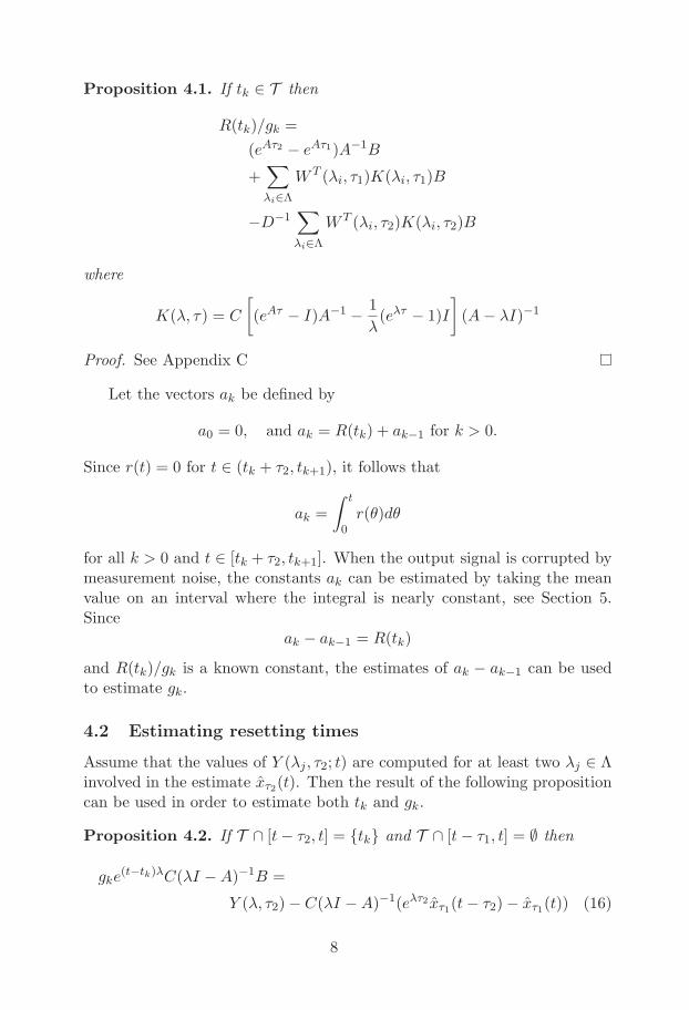
Let the vectors ak be defined by

a0 = 0, and ak = R(tk) + ak−1 for k > 0.

Since r(t) = 0 for t ∈ (tk + τ2, tk+1), it follows that

ak =

∫ t

0r(θ)dθ

for all k > 0 and t ∈ [tk + τ2, tk+1]. When the output signal is corrupted bymeasurement noise, the constants ak can be estimated by taking the meanvalue on an interval where the integral is nearly constant, see Section 5.Since

ak − ak−1 = R(tk)

and R(tk)/gk is a known constant, the estimates of ak − ak−1 can be usedto estimate gk.

4.2 Estimating resetting times

Assume that the values of Y (λj , τ2; t) are computed for at least two λj ∈ Λinvolved in the estimate xτ2(t). Then the result of the following propositioncan be used in order to estimate both tk and gk.

Proposition 4.2. If T ∩ [t− τ2, t] = {tk} and T ∩ [t− τ1, t] = ∅ then

gke(t−tk)λC(λI −A)−1B =

Y (λ, τ2)− C(λI −A)−1(eλτ2 xτ1(t− τ2)− xτ1(t)) (16)

8

Proof. See Appendix D.

Note that the system with two unknowns tk and gk{gke

(t−tk)λ1 = f1gke

(t−tk)λ2 = f2

is uniquely solved by ⎧⎪⎨⎪⎩

tk = ln(f2)−ln(f1)λ1−λ2

+ t

gk = f1e(tk−t)λ1

.

Since each row in (16) can be written in a similar manner, gk and tk canbe evaluated exactly as long as Y (λj , τ2; t) is computed for two distinct λj ,which is the case considered below. However, it is also possible to computeY (λj , τ2; t) for all λj ∈ Λ, and solve the resulting overdetermined system ofequations, e.g. using least-squares techniques. This can be implemented inthe form of the algorithm below.

1. Start while r(t) is zero.

2. Wait for r(t) to become non-zero implying that a resetting event hasoccurred.

3. Wait for time τ1. Now the expression in Proposition 4.2 holds.

4. Compute the right-hand side of (16) for at least two λ and solve fortk and gk, or use estimates of gk and solve only for tk.

Note that it is not necessary to obtain the exact time when r(t) becomesnon-zero. In fact, it suffices that Step 3 of the algorithm is performed at atime t ∈ (tk + τ1, tk + τ2). Thus, in order to reduce sensitivity to noise, onecan carry out Step 3 for several instants t and then use the mean value asan estimate. Logically, the check for a non-zero state estimate residual inStep 1 can be replaced by a check against a suitable threshold.

5 Numerical Example

In this section, the proposed techniques for impulsive input estimation arevalidated on a numerical example.

Assume the following values in model (1)-(3)

A =

[−0.1 00.8 −0.014

], B =

[10

]

C =[0 1

], xTo =

[0 0

]9

with four impacting delta-functions at the time instants T = {5, 80, 160, 230}and with the weights g1 = 0.8, g2 = 0.9, g3 = 0.6 and g4 = 0.7. To evalu-ate the performance of the estimation algorithms under measurement noise,zero mean white noise with variance 0.1 is added to the output of (1)-(3).The output of the plant with noise is shown in Fig. 1.

0 50 100 150 200 250 300−1

0

1

2

3

4

5

6

7

8

t

y

Figure 1: The output signal with measurement noise

For the observer, the time delays are assigned as τ1 = 30 and τ2 = 50,while Λ = {−0.03,−0.08}. Balancing the state-space description with thetransformation x → Tx

T =

[−758.49 27.13163.24 −1.45

],

makes the system satisfy (14) with

D =

[0.18 00 597.39

].

Choosing the elements of Λ closer to zero would reduce the impact of thenoise, but would also probably lead to a larger condition number of D.

For the balanced system, the expression on the right-hand side in Propo-sition 4.1 is

R(tk)

gk=

[−354.85192.24

](17)

From the discussion in Section 4.1, it follows that the integral of r(t) in thenoise-free case is constant on the intervals (tk+τ2, tk+1). The integral of r(t)

10

corrupted by noise can be seen in Fig. 2. The constants ak are approximatedby taking the mean of the red parts in Fig. 2, resulting in the estimatedvalues

a1 =

[−282.99152.99

], a2 =

[−602.17326.25

]

a3 =

[−814.32441.11

], a4 =

[−1062.3575.52

].

Let Gk be the result of element-wise division of ak − ak−1 by the right-handside of (17). Taking the mean of the elements in Gk as estimates for gk gives

g1 = 0.7955, g2 = 0.9016, g3 = 0.5977, g4 = 0.6990

Next both the resetting times tk and the impulse weights gk are estimated

0 50 100 150 200 250 300

−1000

−500

0

R1

t

0 50 100 150 200 250 300

0

200

400

600

R2

t

Figure 2: The integral of r(t). The parts marked with a red line are used tocompute gk.

using the procedure in Section 4.2. The function r(t) is plotted in Fig. 3.In an attempt to decrease the sensitivity to noise, the right hand side of(16) has been computed for all t marked by a red line in Fig. 3. This givesan estimate of gk and tk for each t, and taking the mean value of all theseestimates gives

t1 = 5.22, t2 = 80.06, t3 = 159.87, t4 = 230.12

andg1 = 0.8101, g2 = 0.9104, g3 = 0.5937, g4 = 0.6968.

11

The estimates of gk using this method are slightly worse than those for theintegration method, but here estimates of the resetting times tk are alsogiven.

0 50 100 150 200 250 300−20

−15

−10

−5

0

5

r 1

t

0 50 100 150 200 250 300−2

0

2

4

6

8

r 2

t

Figure 3: The state estimation residual r(t).

6 Conclusion

An observer-based procedure for the estimation of firing times and weightsof Dirac delta-functions impacting a continuous linear time-invariant systemis suggested. The core of the method is in the use of continuous least-squaresobservers implemented by means of a finite memory convolution operator. Anumerical example demonstrates the feasibility of the proposed estimationscheme that is expected to be useful in detecting instants and weights ofpulsatile events in non-basal endocrine secretion.

References

[1] W. M. Haddad, V. Chellaboina, and S. G. Nersesov, Impulsive and Hy-brid Dynamical Systems: Stability, Dissipativity, and Control. Prince-ton: Princeton Univ. Press, 2006.

[2] A. Churilov, A. Medvedev, and A. Shepeljavyi, “Mathematical modelof non-basal testosterone regulation in the male by pulse modulatedfeedback,” Automatica, vol. 45, no. 1, pp. 78–85, 2009.

12

[3] A. Balluchi, L. Benvenuti, M. Di Benedetto, and A. Sangiovanni-Vincentelli, “Design of observers for hybrid systems,” in Hybrid Sys-tems: Computation and Control, ser. Lecture Notes in Computer Sci-ence, C. Tomlin and M. Greenstreet, Eds. Springer Berlin / Heidelberg,2002, vol. 2289, pp. 59–80.

[4] A. Alessandri and P. Coletta, “Switching observers for continuous-timeand discrete-time linear systems,” in American Control Conference,2001. Proceedings of the 2001, vol. 3, 2001, pp. 2516 –2521 vol.3.

[5] E. Medina and D. Lawrence, “State estimation for linear impulsivesystems,” in American Control Conference, 2009. ACC ’09., june 2009,pp. 1183 –1188.

[6] A. Churilov, A. Medvedev, and A. Shepeljavyi, “State observer forcontinuous oscillating systems with pulsatile feedback,” in IFAC WorldCongress, Milano, Italy, September 2011, accepted for presentation.

[7] ——, “Further results on a state observer for continuous oscillatingsystems under intrinsic pulsatile feedback,” in IEEE Conference onDecision and Control, Orlando, FL, December 2011, accepted for pre-sentation.

[8] T. Kailath, Linear Systems. Englewood Cliffs, N.J.: Prentice-Hall,Inc., 1980.

[9] A. Medvedev, “Continuous least-squares observers with applications,”IEEE Transactions on Automatic Control, vol. 41, pp. 1530–1536, 1996.

[10] A. Medvedev and H. T. Toivonen, “Directional sensitivity of continu-ous least-squares state estimators,” Systems & Control Letters, vol. 59,no. 9, pp. 571–577, 2010.

[11] A. Medvedev, “State estimation and fault detection by a bank of con-tinuous finite-memory filters,” International Journal of Control, vol. 69,no. 4, pp. 499–517, 1998.

[12] M. Bask and A. Medvedev, “Analysis of least-squares state estimatorsfor a harmonic oscillator,” in Decision and Control, 2000. Proceedingsof the 39th IEEE Conference on, vol. 4, 2000, pp. 3819 –3824 vol.4.

[13] A. Medvedev, “Disturbance attenuation in finite-spectrum-assignmentcontrollers,” Automatica, vol. 33, no. 6, pp. 1163 – 1168, 1997.

13

A Proof of Lemma 3.1

Assume T ∩ [t− τ, t] = {tk}, and let xo = x(t− τ). Then the state vector isgiven by

x(θ) =

{eA(θ−t+τ)xo if θ ∈ [t− τ, tk)

eA(θ−t+τ)xo + gkeA(θ−tk)B if θ ∈ (tk, t]

Thus

Y (λ, τ ; t) =

∫ t

t−τeλ(t−θ)Cx(θ)dθ

=

∫ t

t−τeλ(t−θ)CeA(θ−t+τ)xodθ + gk

∫ t

tk

eλ(t−θ)CeA(θ−tk)Bdθ.

Both integrals on the right-hand side can be written as

∫ t

aeλ(t−θ)CeA(θ−a)zdθ =

C[eA(t−a) − eλI(t−a)](A− λI)−1z = W (λ, t− a)eA(t−a)z

hence

Y (λ, τ ; t) = W (λ, τ)eAτxo +W (λ, t− tk)eA(t−tk)gkB

and

xτ (t) = V−1τ

∑λi∈Λ

W T (λi, τ)Y (λi, τ) =

eAτxo + V−1τ

∑λi∈Λ

W T (λi, τ)W (λi, t− tk)gkeA(t−tk)B.

From this, and the fact that

x(t) = eAτxo + gkeA(t−tk)B

the result of the proposition follows.

B Proof of Lemma 4.1

Let Vτ1 and Vτ2 correspond to the original system. A state transformationx = Tx results in

Vτ1 = T−TVτ1T−1, Vτ2 = T−TVτ2T

−1.

14

A transformation T such that Vτ1 = I and Vτ2 = D can be found in thefollowing way. Since Vτ1 is symmetric and positive definite there is an or-thogonal U and diagonal L such that

V−1τ1 = ULUT .

Let T1 = L−1/2UT and V = T1V−1τ2 T T

1 . V is symmetric and positive definite,so there exists an orthogonal V and a diagonal D such that

V = V D−1V T .

Now set T = V TL−1/2UT . Then

Vτ1 = T−TVτ1T−1 = I

and

Vτ2 = T−TVτ2T−1 = D.

C Proof of Proposition 4.1

By direct integration it can be verified that

K(λ, τ) =

∫ tk+τ

tk

W (λ, t− tk)eA(t−tk)dt

for any tk. Using Lemma 3.1 it can also be seen that

∫ tk+τj

tk

(x(t)− xτj (t))dt =

gk

∫ tk+τj

tk

eA(t−tk)dtB − gkV−1τj

∑λi∈Λ

W T (λi, τj)K(λi, τj)dtB =

gk

⎡⎣(eAτj − I)A−1 − V−1

τj

∑λi∈Λ

W T (λi, τj)K(λi, τj)

⎤⎦B

Inserting the equation above into

∫ tk+τ2

tk

r(t)dt =

∫ tk+τ2

tk

[−(x(t)− xτ1(t)) + (x(t)− xτ2(t))] dt

proves the proposition.

15

D Proof of Proposition 4.2

Since T ∩ [t− τ2, t] = {tk} it follows, by the same reasoning as in AppendixA, that

Y (λ, τ2; t) =

W (λ, τ2)eAτ2x(t− τ2) + gkW (λ, t− tk)e

A(t−tk)B =

C(A− λI)−1(eAτ2 − eλIτ2

)x(t− τ2) +

C(A− λI)−1gk

(eA(t−tk) − eλI(t−tk)

)B

Noticing thatx(t) = eAτ2x(t− τ2) + gke

A(t−tk)B

then gives

Y (λ, τ2; t) = C(λI −A)−1[gke

λ(t−tk)B + eλτ2x(t− τ2)− x(t)].

This together with the fact that xτ1(t− τ2) = x(t− τ2), xτ1(t) = x(t) whenT ∩ [t− τ2, t] = {tk} and T ∩ [t− τ1, t] = ∅ completes the proof.

16

Paper II

State Estimation in Linear Time-Invariant Systems

With Unknown Impulsive Inputs

Per Mattsson and Alexander Medvedev∗†

Abstract

This paper deals with state estimation in linear time-invariant sys-tems subject to unknown impulsive input signals. A solution based ona linear impulsive observer and a finite-memory convolution operatoris suggested. The problem arises e.g. in the context of systems withintrinsic pulse-modulated feedback that have recently been applied tomathematical modeling of endocrine systems with pulsatile hormonesecretion. Simulation results illustrating the performance of the pro-posed method are provided.

1 Introduction

Mathematical models of dynamical systems with impulsive input signals ap-pear often in mechanics, power electronics and biology, see e.g. [1], mostlyin the applications where impulses represent external momentaneous inter-action. In engineered systems, impulsive control signals are typically knownand therefore can be taken into account in a similar manner as non-impulsiveones. For instance, observer design for this kind of systems is not much dif-ferent from that in a system with any other kind of input signal.

However, in biological applications, the impulsive control signal is oftenunknown. A characteristic example of this class of systems is presentedby the pulsatile endocrine feedback [2]. In [3], a mathematical model forthe non-basal testosterone regulation in the male, based on the concept ofpulse-modulated feedback, is proposed and investigated.

A challenge in devising observers for a system with unknown impulsiveinput signal is that the state variables are reset after a finite time. Thus,most classical asymptotic observers, such as the Luenberger observer [4], lose

∗This research has been supported by the European Research Council (ERC) via theAdvanced Grant 247035 and Grant 2012-3153 from the Swedish Research Council.

†P. Mattsson and A. Medvedev are with Information Technology, Uppsala University,Uppsala, Sweden.

track of the state vector after an impulse. A similar phenomenon occurs withrespect to state estimation in switching system, when the switching time isunknown, as discussed in e.g. [5]. Impulsive observers can be utilized todeal with the state reset problem in impulsive systems.

An impulsive observer that finds the true state in finite time when the in-put is known is presented in [6], and a similar approach is used to implementobserver-based control for systems with persistently acting impulsive inputin [7]. In [8], observers for impulsive systems with linear continuous-timedynamics and a linear resetting law are considered. Further, in [9] and [10],a static gain observer for linear continuous systems under intrinsic impulsivefeedback is studied, and conditions for local stability of the observer underperiodic solutions in the plant are proved.

Unfortunately, most of the existing approaches for designing an impulsiveobserver fail when there is no information about the input impulses. To fillthis gap, an approach to the estimation of impulse times and weights bymeans of continuous least-squares observers is suggested in [11].

The present paper considers impulsive systems with linear continuousdynamics and unknown input impulses. As a solution to the state estimationproblem, a method based on a linear observer coupled with an impulseestimation algorithm, similar to the one in [11], is considered.

The paper is composed as follows. First the equations governing theclass of systems in hand are summarized. Then a general outline of theobserver equations and impulse estimation algorithm is provided, followedby a more detailed explanation of each step. Finally, a numerical exampleillustrating the behaviour of the observer is given.

2 System Equations and Assumptions

Consider the (hybrid) dynamical system with state resets

dx

dt= Ax , t /∈ T (1)

Δx(t) = gkB , t = tk ∈ T (2)

y(t) = Cx(t), (3)

where

Δx(t) = x(t+)− x(t),

x(t+) = limε→0+

x(t+ ε) = x(t) + gkB,

and T is a countable subset of [0,∞), where tk are assumed to be orderedso that t1 < t2 < t3 < . . ..

The instants tk are called impulse times, and to each impulse time, thereis a corresponding impulse weight gk ∈ R. Notice that negative weights areallowed in this formulation. Equations (1)-(2) can be equivalently rewrittenas

x(t) = Ax+Bξ(t),

whereξ(t) =

∑tk∈T

gkδ(t− tk),

and δ(·) is the Dirac delta function. This reformulation clarifies why tk, gkare called impulse time and weight, respectively.

It is assumed that the system has a minimum dwell time Φ, i.e.

0 < Φ ≤ tk+1 − tk

for all k. This is a standard assumption in pulse-modulated systems. Inbiological systems, it is typically motivated by the time required for anorgan or cell to recuperate.

Furthermore, it is assumed that A is a real n×n matrix, C is a real rowvector, B is a real column vector and the matrix pair (A,C) is observable. Itcan be noted that the observer presented in this paper can easily be extendedto also handle known inputs and more than one output.

3 The Observer

In order to estimate the state vector of (1), the impulsive observer

dx

dt= Ax+K(y − y) , t /∈ T (4)

Δx(t) = glB , t = tl ∈ T (5)

y(t) = Cx(t) (6)

will be used, where tl, gl are refereed to as the observer impulse times andweights respectively. Let

D = A−KC.

It is assumed that the observer gain K is chosen so that D is Hurwitz stablewith distinct eigenvalues. Notice that, since (A,C) is observable, it followsthat (D,C) is observable too.

The state estimation error ε(t) = x(t)−x(t) is governed by the equations

dε

dt= Dε , t /∈ T ∪ T , (7)

Δε(t) = gkB , t = tk ∈ T , (8)

Δε(t) = −glB , t = tl ∈ T . (9)

If the impulses in the plant are known, then the observer impulses could bechosen so that tk = tk and gk = gk. In this case the state estimation errorfor t ≥ 0 is given by ε(t) = eDtε(0).

However, in the case investigated in the present paper, the plant impulsesare unknown. To solve the problem with unknown impulses, it is assumedthat, at any time t, the future output values y(·) within a sliding windowy(θ), θ ∈ [t, t+ τ) are made available to the observer. This is possible e.g. ifthe observer is run off-line or the state estimates are allowed to be delayedτ time units. A periodic mode in the plant (as in [9]) also opens up for anapplication of the present technique. Furthermore, it is assumed that τ < Φ,so that there is at most one plant impulse in the sliding window at any timet.

At time t, the observer will utilize a finite-memory convolution operatoron the output y(θ), θ ∈ [t, t + τ), to decide whether or not an observerimpulse should be added in the current interval. If so, the same operator isused to evaluate the observer impulse time and weight.

3.1 Impulsive observer algorithm

A general outline of the algorithm is given next with the details provided inthe subsequent sections.

1. Propagate the observer according to (4), until the condition for addingan observer impulse is met (see Section 3.3). Let to be the time whenthe condition was met.

2. Determine the observer impulse time tl ∈ [to, to + τ) and weight gl.(See Section 3.4.)

3. Propagate the observer according to (4)-(5), until t = to + τ .

4. Go to Step 1.

3.2 The finite-memory convolution operator

In this contribution, the finite-memory convolution operator

(Pf)(λ, τ ; t) =

∫ t

t−τeλ(t−θ)f(θ)dθ (10)

will be utilized. In virtue of being a pseudodifferential operator, (Pf)(λ, τ ; t)is characterized by the symbol

p(λ, τ, s) =1− e(λ−s)τ

s− λ, (11)

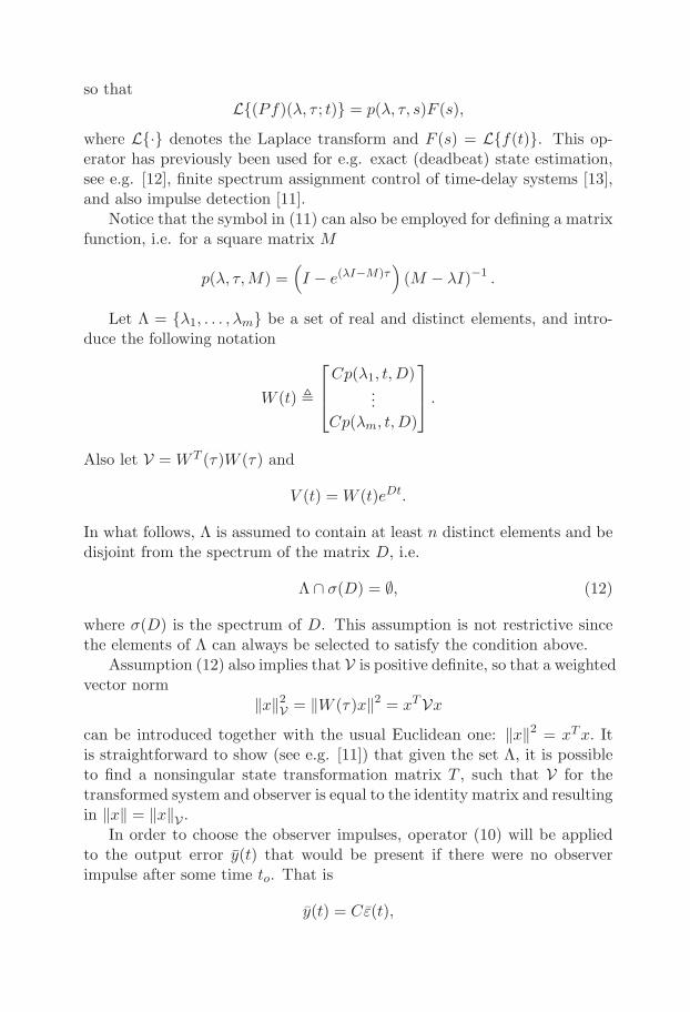
so that

L{(Pf)(λ, τ ; t)} = p(λ, τ, s)F (s),

where L{·} denotes the Laplace transform and F (s) = L{f(t)}. This op-erator has previously been used for e.g. exact (deadbeat) state estimation,see e.g. [12], finite spectrum assignment control of time-delay systems [13],and also impulse detection [11].

Notice that the symbol in (11) can also be employed for defining a matrixfunction, i.e. for a square matrix M

p(λ, τ,M) =(I − e(λI−M)τ

)(M − λI)−1 .

Let Λ = {λ1, . . . , λm} be a set of real and distinct elements, and intro-duce the following notation

W (t) �

⎡⎢⎣Cp(λ1, t,D)

...Cp(λm, t,D)

⎤⎥⎦ .

Also let V = W T (τ)W (τ) and

V (t) = W (t)eDt.

In what follows, Λ is assumed to contain at least n distinct elements and bedisjoint from the spectrum of the matrix D, i.e.

Λ ∩ σ(D) = ∅, (12)

where σ(D) is the spectrum of D. This assumption is not restrictive sincethe elements of Λ can always be selected to satisfy the condition above.

Assumption (12) also implies that V is positive definite, so that a weightedvector norm

‖x‖2V = ‖W (τ)x‖2 = xTVxcan be introduced together with the usual Euclidean one: ‖x‖2 = xTx. Itis straightforward to show (see e.g. [11]) that given the set Λ, it is possibleto find a nonsingular state transformation matrix T , such that V for thetransformed system and observer is equal to the identity matrix and resultingin ‖x‖ = ‖x‖V .

In order to choose the observer impulses, operator (10) will be appliedto the output error y(t) that would be present if there were no observerimpulse after some time to. That is

y(t) = Cε(t),

where ε(t) is the solution to (7)-(8) with the initial value ε(to) = ε(to).Define

R(to) �

⎡⎢⎣(P y)(λ1, τ ; to + τ)

...(P y)(λm, τ ; to + τ)

⎤⎥⎦ . (13)

Notice that y(t), and thus R(to), can be computed if x(to) is known togetherwith the output y(t) for t ∈ [to, to + τ).

Proposition 3.1. If T ∩ [to, to + τ) = {tk}, then

R(to) = V (τ)ε(to) + gkV (to + τ − tk)B,

and if T ∩ [to, to + τ) = ∅, then

R(to) = V (τ)ε(to).

Proof. Cf. Appendix I in [11].

Proposition 3.1 shows in what way R(t) is affected when a plant impulseenters the sliding window [t, t + τ). It is also of interest to see how R(t) isrelated to the state estimation error ε(t).

Proposition 3.2. Assume that T ∩ [to, to+ τ) = {tk} and T ∩ [to, to+ τ) ={tl}. Then

W (τ)ε(to + τ) = V (τ)ε(to)

+ gk (V (to + τ − tk)B + E(tk − to)) (14)

− gl(V (to + τ − tl)B + E(tl − to)

),

whereE(t) = (W (τ)−W (τ − t))eD(τ−t)B.

Furthermore, for any ε, r > 0, it is possible to choose the set Λ such thateach row of V (to + τ − t)B and E(t− to) satisfy

|Ei(t− to)| ≤ r|Vi(to + τ − t)B|

when t− to ≤ τ − ε.

Proof. See Appendix A.

Proposition 3.2 justifies the following important approximation. If Λ ischosen such that the proposition holds for a small enough r, and there areno impulses in [to+τ−ε, to+τ), then the terms gkE(tk− to) and glE(tl− to)in (14) are negligible. Thus it follows from Proposition 3.1 that

W (τ)ε(to + τ) ≈ R(to)− glV (to + τ − tl). (15)

3.3 Step 1: Deciding on observer impulse

This section deals with the first step in the impulsive observer algorithmof Section 3.1. In this step, the observer propagates the state estimationx(t) according to (4) and computes R(t), defined in (13), for each t. Thiscontinues until some time to, when it is decided that there should be anobserver impulse in the interval [to, to + τ).

In order to see whether or not an observer impulse should be added,‖R(t)‖ will be considered. Notice that if ε(t) = 0 and T ∩ [t, t + τ) = ∅,then it follows from Proposition 3.1 that R(t) = 0. However, as soon as animpulse at tk enters the sliding window [t, t+ τ), the norm of R(t) will startto increase according to the relationship

‖R(t)‖ = |gk| ‖V (t+ τ − tk)B‖ , 0 < tk − t < τ. (16)

Thus, if ‖R(t)‖ > 0, then ε(t) �= 0 and/or T ∩ [t, t+ τ) �= ∅. In both cases,there is a reason to add an observer impulse. If ε(to) �= 0, then the observerimpulse could be used to reduce the state estimation error, and if there is aplant impulse within [t, t + τ), then the observer should counter it with anobserver impulse.

Thus, a condition for choosing to is that ‖R(to)‖ > 0. For robustnesssake, zero in the right-hand side of the inequality can be replaced by

‖R(to)‖ > η,

for some threshold η > 0.It is also desirable, as motivated in Section 3.4, that (15) holds at time

to. Due to Proposition 3.2, it is thus preferable to choose to so that thereis no plant impulse in [to + τ − ε, to + τ), and the designer should take thisinto account when picking η.

Since the way in which ‖R(t)‖ is affected by an impulse is known before-hand, this is usually not a problem, at least when some bounds on |gk| areknown. For instance, the interval of admissible impulse weights is alwaysknown in pulse-modulated control. Notice that if |gk| ≤ gM for all k, thenη could be chosen so that

η > gM∥∥V (τ − t)B

∥∥ , for τ − ε < t < τ,

cf. (16). However, if η is chosen too large, small impulses might be missed.It is often possible to devise a more advanced condition for choosing to,

by studying the graph of

‖V (τ − tk)B‖ , 0 < tk < τ.

In this way it might be possible to choose to in a way that does not dependon the impulse weights. An example of this is provided in Section 4.

3.4 Step 2: Evaluating the observer impulse

This section deals with the second step in the impulsive observer algorithmof Section 3.1.

Suppose that it has been decided at time to that there should be anobserver impulse in [to, to + τ), see Section 3.3. Let εo = ε(to). Assume alsothat there is a plant impulse with weight gk at time tk ∈ [to, to + τ). If thisis not the case, then gk = 0 throughout this section.

When εo = 0, it follows from Proposition 3.1 that tk and gk can be foundby solving

R(to) = glV (to + τ − tl)B. (17)

However, for εo �= 0, the above equation may not have a solution. Therefore,the following optimization problem is solved instead

mintl,gl

∥∥R(to)− glV (to + τ − tl)B∥∥2 ,

s.t to < tl < to + τ.(18)

A suitable technique for solving this problem is discussed in Section 3.5.For εo = 0, (17) is always satisfied by choosing tl = tk and gl = gk.

Numerical experiments indicate that this solution is also unique, but thisresult is not formally proved here.

To analyze what happens when εo �= 0, assume that an observer impulseis fired at tl. If Λ has been chosen so that Proposition 3.2 holds for a smallenough r, and there is no impulse in [to + τ − ε, to + τ) (see Section 3.3),then it can be concluded from (15) that

‖ε(to + τ)‖2V ≈∥∥R(to)− glV (to + τ − tl)B

∥∥2 . (19)

The right-hand side of (19) is exactly the quantity that is minimized in (18).Also note that thanks to the minimization,∥∥R(to)− glV (to + τ − tl)B

∥∥ ≤∥∥eDτεo

∥∥V .

Hence, if εo �= 0, the observer might add an impulse that does not correspondto an impulse in the plant. However, in this case the “false” impulse is chosenso that

‖ε(to + τ)‖V �∥∥eDτεo

∥∥V

where the right-hand side is the state estimation error that is acquired whenthe observer impulse coincides with the plant impulse.

In practice, the observer usually adds “false” impulses when the stateestimation error is large, resulting in a faster convergence (see also Section 4).As the state estimation error decays over time, the observer impulses willget closer to the true plant impulses, as seen in Section 4.

3.5 Solving the optimization problem

Solving optimization problem (18) is an important part of the observer de-scribed above. Notice that the cost function depends linearly on gl. Itfollows that, if the pair tl, gl minimizes the cost function in (18) then

gl = (BTV TV B)−1BTV TR(to),

where V = V (to + τ − tl). Inserting this into (18) gives rise to a nonlinearoptimization problem in one variable. Thanks to the constraint tl ∈ [to, to+τ), this problem can be solved with an arbitrary accuracy by gridding theinterval, evaluating the cost function at each point, and selecting the solutionthat corresponds to the least cost function value.

3.6 The observer parameters

Besides the condition discussed in Section 3.3 (e.g. choosing the thresholdη), the designer has to choose the observer gain matrix K, the length of thesliding window τ , and the set Λ.

The proof of Proposition 3.2 shows that letting the elements of Λ tend tonegative infinity ensures that the approximation in (15) is valid. However,other aspects have also to be taken into account. In [13] and [11], the low-pass characteristics and disturbance attenuation of the operator (10) arestudied. It is demonstrated that the operator in general is less sensitiveto measurement noise when |λ| is small. Thus there is a trade-off betweenmaking r in Proposition 3.2 small, and decreasing the sensitivity to noise.Fortunately, this trade-off can usually be handled in practice, as shown inSection 4. It is also seen that the sensitivity to high frequency noise isreduced when τ is increased. However, increasing τ leads to a longer lagin the state estimate. Furthermore, τ must be chosen less than Φ, whichlimitation is set by the plant characteristics.

Following [14], it is also of interest to study the sensitivity of (10) tostructured uncertainty in the system matrix of the plant, and how it isinfluenced by the choice of Λ and τ .

Finally, the observer gain K has to be selected. This will mainly affectthe state estimates behaviour in between impulses, and could be chosen e.g.as in a (steady-state) Kalman filter.

4 Numerical Example

In this section, the proposed technique for state estimation is validated on anumerical example, both with and without measurement noise. The observer

is applied to sampled data, with fast sampling (0.01 time units between eachsample), to imitate continuous execution.

Assume the following values in (1)-(3)

A =

⎡⎣−0.08 0 0

2 −0.15 00 0.5 −0.2

⎤⎦ , B =

⎡⎣100

⎤⎦

C =[0 0 1

], xo =

⎡⎣ 42060

⎤⎦

with four impacting impulses

t1 = 10 t2 = 40, t3 = 80 t4 = 140

g1 = 4 g2 = 5 g3 = 7 g4 = 6.

To see the effect of measurement noise, white noise of zero mean and variance10 was added to the output. The output y(t) of the system is shown in Fig.1. For the observer, the gain was chosen as

K =

⎡⎣0.00020.00480.0200

⎤⎦ ,

so that the eigenvalues of D are placed at −0.1,−0.15 and −0.2. The lengthof the sliding window was set to τ = 20. Finally, Λ was chosen as

Λ = {−2.65,−2.70,−2.75,−2.80,−2.85,−2.90}.

For this set of parameters, it holds that

|Ei(t− to)| < 10−7|Vi(to + τ − t)B|,

when t− to ≤ 15, cf. Proposition 3.2.Thus, if the optimization problem in (18) is only solved when T ∩ [to +

15, to + 20) = ∅, then (19) is a good approximation.Next a condition for adding an observer impulse should be chosen. In

light of the discussion in Section 3.3, first consider ‖V (to + τ − tk)B‖, whichquantity is plotted in Fig. 2. The maximum in Fig. 2 occurs when tk− to ≈5.8, i.e. well below 15. This suggests choosing the optimization instants toin the observer such that the quantity ‖R(t)‖ is at, or near, a maximum.Also, with this condition, the chosen optimization instants will not dependon the impulse weights. Hence, in this example, Step 1 of the algorithm inSection 3.1 will continue until ‖R(t)‖ reaches a maximum.

0 20 40 60 80 100 120 140 160 180 200−20

0

20

40

60

80

100

120

Time, t

y(t)

Figure 1: The output signal of the plant, with noise (blue line) and without(red line).

First the noise-free output was tested. In Fig. 3, the state estimatesproduced by the observer initialized with

x(0) =

⎡⎣ 73070

⎤⎦

are shown together with true values of the plant states. The state estimationerror x(t)− x(t), together with the quantity eDt(x(0)− x(0)) are provided inFig. 4. The latter characterizes the state estimation error that the observerwould have with all observer impulses being identical to the plant impulses.

It can be seen that the proposed observer is completely off on the firstimpulse, but yet converges to the true state vector faster than it would ifthe first impulse were identical to the true plant impulse.

The observer was also tested with white measurement noise of variance10 added to the output, see Fig. 1. The resulting state estimation error ispresented in Fig. 5. Obviously, the estimated impulses are quite far fromthe true ones because of the measurement noise. In Section 3.6 it is seenthat one way to reduce the sensitivity to noise is to move the elements of Λ

0 5 10 15 200

2

4

6

8

10

12

t− to

‖V(to+τ−t)B

‖

Figure 2: ‖V (to + τ − tk)B‖ for 0 < tk − to < τ .

closer to the origin. Therefore, the observer was also tested with

Λ = {−0.65,−0.70,−0.75,−0.80,−0.85,−0.90}

and the rest of the parameters left unchanged. The result for these parame-ters, with the noisy measurements of the output, is shown in Fig. 6. Clearly,the estimated impulses are much closer to the actual impulses in this case.

5 Conclusion

An observer for state estimation in linear time-invariant systems with un-known input impulses is suggested. The core of the method is to use a stan-dard linear observer coupled with a state estimation algorithm employingfinite-memory convolution operators. A numerical example demonstratesthe feasibility of the proposed observer.

0 50 100 150 2000

5

10

x1

0 50 100 150 2000

50

x2

0 50 100 150 2000

50

100

150

x3

Time, t

Figure 3: True states x(t) (blue line), and estimated states x(t) (red line).

0 50 100 150 2000

5

|ε1|

0 50 100 150 2000

10

20

30

|ε2|

0 50 100 150 2000

50

|ε3|

Time, t

Figure 4: State estimation error |x(t) − x(t)| (blue line), and the state es-timation error for an observer with exact knowledge of the plant impulses(red line).

0 50 100 150 2000

5

10|ε

1|

0 50 100 150 2000

102030

|ε2|

0 50 100 150 2000

50

|ε3|

Time, t

Figure 5: State estimation error |x(t) − x(t)|, with original Λ, when mea-surement noise is added to the output.

0 50 100 150 2000

5

|ε1|

0 50 100 150 2000

10

20

30

|ε2|

0 50 100 150 2000

50

|ε3|

Time, t

Figure 6: State estimation error |x(t) − x(t)|, with modified Λ, when mea-surement noise is added to the output.

References

[1] W. Haddad, V. Chellaboina, and S. Nersesov, Impulsive and HybridDynamical Systems: Stability, Dissipativity, and Control, ser. PrincetonSeries in Applied Mathematics. Princeton University Press, 2006.

[2] W. S. Evans, L. S. Farhy, and M. L. Johnson, “Biomathematical mod-eling of pulsatile hormone secretion: a historical perspective,” in Meth-ods in Enzymology: Computer methods, Volume A, M. L. Johnson andL. Brand, Eds., 2009, vol. 454, pp. 345–366.

[3] A. Churilov, A. Medvedev, and A. Shepeljavyi, “Mathematical modelof non-basal testosterone regulation in the male by pulse modulatedfeedback,” Automatica, vol. 45, no. 1, pp. 78–85, 2009.

[4] D. Luenberger, “Observers for multivariable systems,” IEEE Transac-tions on Automatic Control, vol. 11, no. 2, pp. 190–197, apr 1966.

[5] Y. Tian, T. Floquet, L. Belkoura, and W. Perruquetti, “Algebraicswitching time identification for a class of linear hybrid systems,” Non-linear Analysis: Hybrid Systems, vol. 5, no. 2, pp. 233 – 241, 2011.

[6] T. Raff and F. Allgower, “An impulsive observer that estimates theexact state of a linear continuous-time system in predetermined finitetime,” in Mediterranean Conference on Control Automation, june 2007,pp. 1–3.

[7] G. Zheng, Y. Orlov, W. Perruquetti, and J.-P. Richard, “Finite-timeobserver-based control of linear impulsive systems with persistently act-ing impact,” in IFAC World Congress, Milano, Italy, Aug. 2011.

[8] E. Medina and D. Lawrence, “State estimation for linear impulsivesystems,” in American Control Conference, june 2009, pp. 1183–1188.

[9] A. Churilov, A. Medvedev, and A. Shepeljavyi, “A state observer forcontinuous oscillating systems under intrinsic pulse-modulated feed-back,” Automatica, vol. 48, no. 6, pp. 1117–1122, 2012.

[10] ——, “Further results on a state observer for continuous oscillatingsystems under intrinsic pulsatile feedback,” in 50th IEEE Conference onDecision and Control and European Control Conference (CDC-ECC) ,dec. 2011, pp. 5443–5448.

[11] P. Mattsson and A. Medvedev, “Estimation of input impulses by meansof continuous finite memory observers,” in American Control Confer-ence, june 2012, pp. 6769–6774.

[12] A. Medvedev, “Continuous least-squares observers with applications,”IEEE Transactions on Automatic Control, vol. 41, no. 10, pp. 1530–1537, oct 1996.

[13] ——, “Disturbance attenuation in finite-spectrum-assignment con-trollers,” Automatica, vol. 33, no. 6, pp. 1163–1168, 1997.

[14] A. Medvedev and H. T. Toivonen, “Directional sensitivity of continu-ous least-squares state estimators.” Systems & Control Letters, vol. 59,no. 9, pp. 571–577, 2010.

A Proof of Proposition 3.2

The relation in (14) follows from the fact that

ε(to + τ) = eDτε(to) + gkeD(to+τ−tk)B − gle

D(to+τ−tl)B.

To prove the last part of the proposition assume, without loss of gener-ality, that to = 0.

Let Ci = C(λiI −D)−1. The rows of E(t) are given by

Ei(t) = Ci

(e(λiI−D)τ − e(λiI−D)(τ−t)

)eD(τ−t)B =

eλi(τ−t)Ci

(e(λiI−D)t − I

)B.

Notice that, for fixed t > 0,∣∣∣Ci(e(λiI−D)t − I)B

∣∣∣ → 0, as λi → −∞.

Similarily, the rows of V (τ − t)B are found to be

Vi(t)B = Ci

(e(λiI−D)(τ−t) − I

)eD(τ−t)B =

− eλi(τ−t)Ci

(e(D−λiI)(τ−t) − I

)B.

Note that, for fixed 0 < t < τ ,∣∣∣Ci(e(D−λiI)(τ−t) − I)B

∣∣∣ → ∞, as λi → −∞.

Hence, it can be concluded that, for 0 < t < τ ,

|Ei(t)||Vi(t)B|

=|Ci(e

(λiI−D)t − I)B||Ci(e(D−λiI)(τ−t) − I)B|

→ 0, as λi → −∞

and thus the result of the proposition follows.

Paper III

Periodical Solutions in a Pulse-modulated Model of

Endocrine Regulation with Time-delay

Alexander Churilov, Alexander Medvedev, and Per Mattsson∗†‡

Abstract

A hybrid mathematical model of endocrine regulation obtainedby augmenting the classical continuous Smith model with a pulse-modulated feedback to describe episodic (pulsatile) secretion is consid-ered. Conditions for existence and local orbital stability of periodicalsolutions with m impulses in the least period (m-cycles) are derived.An important implication of the performed analysis is that the nonlin-ear dynamics of the pulse-modulated system and not the delay itselfcause the sustained closed-loop oscillations. Furthermore, simulationand bifurcation analysis indicate that increasing the time delay in thesystem in hand typically, but not always, leads to less complex dy-namic pattern in the closed-loop system by giving rise to stable cyclesof lower periodicity.

1 Introduction

Hormones are the signaling substances of endocrine systems that regulatemany aspects in the human body, i.e. metabolism, growth as well as thesexual function and the reproductive processes. Hormones are secreted byendocrine glands directly into the bloodstream in continuous (basal) or pul-satile (non-basal) manner. Endocrine glands, interacting via hormone con-centrations in blood, build up dynamical control loops characterized by self-sustained oscillations of the involved physiological quantities, [1].

Oscillations in biological feedback systems arise for a broad range of sys-tem parameters which property is not always captured by the mathematicalmodels, [2]. With respect to mathematical models of endocrine regulation,

∗A. Medvedev and P. Mattsson were in part financed by the European Research Coun-cil, Advanced Grant 247035 (SysTEAM).

†A. Churilov is with the Department of Mathematics and Mechanics, St. PetersburgState University, St. Petersburg, Russia.

‡A. Medvedev and P. Mattsson are with Information Technology, Uppsala University,Uppsala, Sweden.

1

mostly nonlinear feedback and time delays were employed for achieving sus-tained periodical solutions. The Smith model of testosterone regulation [3]is proven to be asymptotically stable for any value of the time delay and thenonlinear feedback in the form of a first-order Hill function, [4]. However,under piecewise linear (affine) feedback nonlinearities, multiple periodicalorbits and chaos arise in the Smith model [5, 6]. Multiple delays in theSmith model under a second-order Hill function feedback are also shownto lead to sustained nonlinear oscillations in some subspaces of the modelparameters [7]. Naturally, the equilibrium point of the model dynamics hasto be rendered unstable.

The concept of amplitude and frequency pulse-modulated feedback ap-pears naturally in non-basal hormone regulation and is widely accepted. Therationale is given e.g. in [8]. A hybrid parsimonious mathematical modeldescribing pulsatile endocrine regulation and lending itself to mathematicalanalysis is suggested in [9] and studied in detail in [10]. The model does not,by design, have any equilibria and always possesses a 1-cycle, i.e. a periodicsolution with one pulse in the least period. It is also shown to exhibit com-plex nonlinear dynamics such as cycles of higher periodicity and chaos [11].The latter discovery confirms that the pulse-modulated model in question isable to produce signaling patterns of any dynamical complexity. However,in its original formulation, the pulse-modulated model of hormone secretiondoes not take into account the presence of a time delay in the closed loopthat is a significant phenomenon in many endocrine systems. Time delay ispresent in endocrine systems mainly due to two circumstances. First, thereis a delay due to the transport of the hormones in the blood stream. Second,a delay also results from the lack of releasable pools of the hormone and theneed to synthesize it before secretion [8].

With the time delay taken into account, the pulse-modulated model ofendocrine regulation acquires an infinite-dimensional continuous part. Theclosed-loop dynamics are therefore both hybrid and infinite dimensional,which combination is mathematically challenging and so far rarely treated.The existing theory of impulsive delay-differential equations (see, e.g., [12,13]) does not readily provide the tools for an exhaustive analysis of themodel under consideration. The present study is therefore aimed to fillthe existing gap in mathematical modeling of non-basal endocrine feedbackregulation and provide insights into the dynamical phenomena occurring inpulse-modulated models of such systems due to the time delay.

In this paper, existence and stability conditions for periodical solutionsin a time-delay pulse-modulated model of non-basal endocrine regulationare derived in a general mathematical framework and specialized to the caseof testosterone regulation in the human male. The paper is organized asfollows. First a brief background on linear time-delay systems is provided

2

and the notion of finite-dimension reducible system is introduced. Then a(hybrid) model describing a continuous time-delay system controlled by apulse-modulated feedback is formulated, followed, under the assumption offinite-dimensional reducibility, by a detailed analysis of existence and sta-bility of the closed-loop behaviors. Finally, the obtained theoretical resultsare applied to the case of non-basal testosterone regulation in the male andvalidated through simulation and numerical calculations.

2 Finite-Dimension Reducible Linear Time DelaySystems

Consider an autonomous time-delay system

dx

dt= A0x(t) +A1x(t− τ), (1)

where x(t) ∈ Rp is the state vector, A0, A1 ∈ R

p×p are square constantmatrices, A1 �= 0, and τ �= 0 is a constant time delay. System (1) is subjectto the initial conditions x(t) = ϕ(t), −τ � t � 0, where ϕ(t) is a continuousvector function.

The following property of time-delay systems is of principal importancefor the exposition.

Definition 1. Time-delay linear system (1) is called finite-dimension re-ducible (FD-reducible) if

A1Ak0A1 = 0 for all k = 0, 1, . . . , p− 1. (2)

The property of FD-reducibility is not particularly liming when it comesto endocrine systems. Indeed, a simple endocrine axis typically constitutesa cascade coupling of non-oscillatory blocks representing the concentrationsof individual hormones with time delays in between. In such a system, FD-reducibility is equivalent to the lack of local feedback around the time-delayblock.

Obviously, relationships (2) can be equivalently rewritten as

A1eA0tA1 = 0 for all t � 0. (3)

Lemma 1. System (1) is FD-reducible iff there exists an invertible p × pmatrix S such that

S−1A0S =

[U 0W V

], S−1A1S =

[0 0W 0

], (4)

where the blocks U , V are square, the sizes of the blocks W and W are equal,and the matrix pair (W , U) is observable (see, e.g., [14]).

3

The theorem can be proved by state space transformation, [14]. Theblock structure of the matrices in (4) clearly relates to the models of en-docrine systems with time delay between the compartments and is often en-countered in endocrine axes with feedback non-basal regulation, see e.g. [15].Under the assumption of FD-reducibility, system (1) posesses a cascade(feedforward) structure comprising finite-dimensional blocks revealed by theblock-triangular structure of the transformed matrix A0 in (4) and intercon-nected by a pure time delay, as implied by the nilpotent A1.

Corollary 1. Let system (1) be FD-reducible. Then for any complex s andany real τ one has

det(A0 +A1e−τs − sIp) = det(A0 − sIp).

The result follows from the block structure specified in (4). Thus thespectrum of an FD-reducible system (1) is finite and independent of thedelay τ . Time-delay systems with finite spectrum appear e.g. in the classicalcontrol problem of finite spectrum assignment, see [16, 17].

Introduce the matrix D = A0 + A1e−A0τ . Following [18], consider a

fundamental solution of (1), namely a function X(t, t0) with the properties:X(t, t0) = 0 for t < t0, X(t0, t0) = Ip, and

∂X

∂t= A0X(t, t0) +A1X(t− τ, t0) for t � t0. (5)

Theorem 1. Let system (1) be FD-reducible. Then X(t, t0) = H(t−t0)Ψ(t−t0), where

Ψ(t) =

{eA0t, t � τ,

eD(t−τ)eA0τ , t � τ,(6)

and H(t) is the Heaviside step function. (Here H(0) = 1.)

Proof. From the block representation in (4), any solution x(t) of (1) satisfiesthe linear differential equation

dx

dt= Dx (7)

for t � τ . Then (6) follows immediately.

It is seen from (7) that time-delay system (1) behaves as a finite-dimensionalsystem of dimension p on the time interval [τ,+∞) while its infinite-dimensionalnature is revealed only on the segment [0, τ ].

Lemma 2. The following relationships are true:

A1Ψ(t) = A1eA0t, Ψ(t)A1 = eA0tA1 for all t. (8)

4

Proof. Lemma 2 is a straightforward consequence of Theorem 1 and Lemma 1and follows from the block representation (4).

Introduce, for further use, the matrix functions

Ψ0(t) = H(t− τ)eA0(t−τ)

and

Q(t, ξ) =

∫ 0

−τΨ0(t− θ)A1e

A0(θ+ξ) dθ,

Q0(t, ξ) = eA0(t−τ)(eDτ − eA0τ

)eA0ξ.

(9)

Lemma 3. The following relationship holds:

Q(t, ξ) =

{(eDt − eA0t

)eA0ξ, t � τ,

Q0(t, ξ), t � τ.

Proof. By using the block form (4) of the matrices A0, A1 it can be shownthat if system (1) is FD-reducible, then

∫ t

t0

eA0(t−θ)A1eA0(θ−t0)dθ =

(eD(t−t0) − eA0(t−t0)

)eA0τ (10)

for any real t, t0. Clearly, the matrix function Q(t, ξ) can be written as

Q(t, ξ) =

∫ min{t−τ,0}

−τeA0(t−τ−θ)A1e

A0(θ+ξ) dθ.

Now Lemma 3 follows from (10).

From (3), (9) and Lemma 3, it is seen that

A1Q(t, ξ) = A1Q0(t, ξ) ≡ 0 for all t, ξ. (11)

Lemma 4. Let x(t) be a solution of an FD-reducible system (1) and t0 � 0.Then

x(t) = Ψ(t− t0)x(t0) +

∫ 0

−τΨ0(t− t0 − θ)A1x(θ + t0) dθ (12)

for t � t0.

Proof. From [18] one has

x(t) = X(t, t0)x(t0) +

∫ t0

t0−τX(t, θ + τ)A1x(θ) dθ (13)

5

for t � t0. From Theorem 1, it follows that

x(t) = Ψ(t− t0)x(t0) +

∫ t0

t0−τH(t− τ − θ)Ψ(t− τ − θ)A1x(θ) dθ (14)

for t � t0. Then (14) and the second equality in (8) imply the sought resultof the lemma.

Next, an alternative description of the evolution operator generated by(1) is provided.

Lemma 5. Let x(t) be a solution of an FD-reducible system (1). Pick twonumbers t0, t1 satisfying t0 � 0 and t1 − t0 � τ . Then, it holds that

x(t) = Ψ(t− t1)x(t1) +Q(t− t1, t1 − t0)x(t0) (15)

for t � t1.

Proof. It follows from (12) that

A1x(t) = A1Ψ(t− t0)x(t0) for t � t0.

Due to Lemma 4

x(t) = Ψ(t− t1)x(t1) +

∫ 0

−τΨ0(t− t1 − θ)A1x(θ + t1) dθ, (16)

for t � t1. Hence, for t1 − τ � t0, (16) can be rewritten as

x(t) = Ψ(t− t1)x(t1) +

∫ 0

−τΨ0(t− t1 − θ)A1Ψ(θ + t1 − t0) dθ x(t0).

Then Lemma 5 follows from (9).

The relationship (15) shows that a solution x(t) satisfying (1) for t � t1is completely defined by two initial finite-dimensional vectors, i.e. x(t0) andx(t1). This property is in contrast with general time-delay systems of type(1) and explains the name of the above introduced notion of FD-reducibility.

3 A Time-Delay Impulsive System

Consider an extension of the impulsive model of non-basal endocrine reg-ulation treated iN [9, 10] to the class of systems with delayed continuouspart:

dx

dt= A0x(t) +A1x(t− τ), y = Cx,

tn+1 = tn + Tn, x(t+n ) = x(t−n ) + λnB,

Tn = Φ(y(tn)), λn = F (y(tn)).

(17)

6

where B is a vector and C is a row such that CB = 0. Thus, the signal thatis fed back through the pulse-modulated feedback is scalar. The relationshipbetween C and B safeguards the continuity of the output y. Without lossof generality assume t0 = 0. For brevity sake denote xn = x(t−n ).

Model (17) is effectively a so-called Smith model [19] with a pulse-modulated feedback.

The continuous functions Φ(·), F (·), representing respectively frequencyand amplitude modulation [20], satisfy

0 < Φ1 � Φ(·) � Φ2, 0 < F1 � F (·) � F2, (18)

for some constants Φi, Fi, i = 1, 2. The latter condition implies that system(9) has no equilibria and thus eliminates the main shortcoming of the clas-sical Smith model, see [4]. In the context of endocrine system, the functionΦ(·) defines the time instants when hormone pulses are fired while F (·) isused to evaluate their magnitudes.

Since the linear part of the system represents the kinetics of the involvedhormones, it has to be stable, i.e., all the roots of the characteristic equationdet(sIp − A0 − A1e

−τs) = 0 have to satisfy Re s < 0. Furthermore, thecontinuous part of system (17) is henceforth assumed to be FD-reducible.Then, as it follows from Corollary 1 to Lemma 1, stability of the linear partof (17) is ensured by Hurwitz stability of the matrix A0.

Besides of stability of the continuous part of the model under considera-tion, it is also biologically feasible that all the solutions of (17) are bounded.The bondedness of all the solutions for t � 0 follows from inequality (18)and from the FD-reducibility (namely, from representation (4)).

Lemma 6. Assume that

infyΦ(y) > τ (19)

and the initial function ϕ(t), −τ � t � 0 is continuous. Then (17) issatisfied by x(t) defined as follows.

For 0 < t < t1,

x(t) = Ψ(t)(x0 + λ0B) +

∫ 0

−τΨ0(t− θ)A1ϕ(θ) dθ. (20)

For n � 1 and tn < t < tn+1,

x(t) = Ψ(t− tn)(xn + λnB) +Q(t− tn, Tn−1)(xn−1 + λn−1B), (21)

where the function Q(t, ξ) is given by (9).

7

Proof. From Lemma 4 for tn < t < tn+1, n � 0

x(t) = Ψ(t− tn)x(t+n ) +

∫ 0

−τΨ0(t− tn − θ)A1x(θ + tn) dθ. (22)

Since t0 = 0, (22) implies (20) for n = 0.From (3), (8) and (22) it is concluded that

A1x(t) = A1eA0(t−tn)(xn + λnB), tn < t < tn+1. (23)

Consider n � 1. Then from (19) tn−1 < tn − τ � tn + θ � tn as−τ � θ � 0. Hence from (23)

A1x(tn + θ) = A1eA0(tn+θ−tn−1)(xn−1 + λn−1B) (24)

for −τ � θ � 0. Substitute (24) into (22) to obtain (21).

4 A Discrete-Time System

In this section, it is demonstrated that impulsive system (17) with an FD-reducible continuous part can be described by discrete dynamics at the in-stants tn, n = 0, 1, . . . .

Define a matrix function P (x, z) that maps p-dimensional vectors x andz into a p-dimensional vector

P (x, z) = Ψ(Φ(Cx))[x+ F (Cx)B]

+Q0(Φ(Cx),Φ(Cz))[z + F (Cz)B],(25)

where Q0(t, ξ) is given by (9). Consider a sequence of vectors xn = x(t−n ).Introduce also

Tn = Φ(Cxn), λn = F (Cxn), n = 0, 1, . . . .

In particular,T0 = Φ(Cϕ(0)), λ0 = F (Cϕ(0)),

where ϕ(t) is the initial function of (17).

Lemma 7. Let (19) be satisfied and ϕ(t), −τ � t � 0 be a continuous initialfunction. Then the vectors xn satisfy the recursion

xn+1 = P (xn, xn−1), n � 1, (26)

with the initial values x0 = ϕ(0),

x1 = Ψ(T0)(x0 + λ0B) + eA0(T0−τ)

∫ 0

−τe−A0θA1ϕ(θ) dθ. (27)

8

Proof. Equations (27), (26) are obtained by setting t = t1 in (20) and t =tn+1 in (21), respectively. Since by (19) tn+1 − tn > τ , due to Lemma 3, Q0

can be substituted by Q.

For discrete time dynamical system (26), the sequence x0, x1, x2, . . .,can be termed as the forward orbit of the initial point (x0, x1).

Notice that, contrary to the delay-free case considered in [10], the knowl-edge of the sequence xn is not sufficient to reconstruct the inter-impulsebehavior of the continuous time system solution x(t). Indeed, in general,the initial function ϕ(t) cannot be uniquely found from integral equation(27). However, it will be shown in the next section that such reconstructionbecomes possible provided x(t) is periodic.

5 Existence of Cycles

The existence conditions for periodic solutions with m impulses in the leastperiod (m-cycles) of pulse-modulated time delay system (17) are investigatedin this section. Evidently, every such solution gives rise to an m-periodicforward orbit of discrete map (26). It will be shown below that the conversestatement is also true: every m-periodic orbit corresponds to a unique initialfunction for a solution with m impulses in the least period.

Let the matrix functions Q(t, ξ), Q0(t, ξ) be as in (9).

Theorem 2 (existence of a 1-cycle). Let (19) be satisfied. Suppose thatthere exists a vector x0 such that

x0 = [Ψ(T0) +Q0(T0, T0)] (x0 + λ0B), (28)

where T0 = Φ(Cx0), λ0 = F (Cx0). Then there exists a T0-periodic 1-cyclewith the initial function defined by

ϕ(t) = [Ψ(t+ T0) +Q(t+ T0, T0)] (x0 + λ0B), −τ � t � 0. (29)

Conversely, if there exists a 1-cycle then the vector x0 = ϕ(0) satisfies (28)with the initial function ϕ(t) given by (29).

Proof. To obtain a 1-cycle it suffices to ensure that

x(t+ T0) = ϕ(t), −τ � t < 0.

By means of (20) this can be rewritten for −τ � t < 0 as

ϕ(t) = Ψ(t+ T0)(x0 + λ0B) +

∫ 0

−τΨ0(t+ T0 − θ)A1ϕ(θ) dθ . (30)

9

Multiply (30) by A1 from the left. Then

A1ϕ(t) = A1Ψ(t+ T0)(x0 + λ0B) = A1eA0(t+T0)(x0 + λ0B)

for −τ � t < 0. Substitute the last equality into (30) to get

ϕ(t) =

[Ψ(t+ T0) +

∫ 0

−τΨ0(t+ T0 − θ)A1e

A0(θ+T0) dθ

]× (x0 + λ0B), −τ � t < 0,

which yields (29). Setting t = 0 in (29) and employing (28) gives ϕ(0) =x0.

Theorem 3 (existence of an m-cycle). Let (19) be satisfied. Consider aninteger number m � 2. Suppose that there exist vectors x0, . . . , xm−1 suchthat xi �= xj for i �= j and

x0 = P (xm−1, xm−2),

x1 = P (x0, xm−1),

xn = P (xn−1, xn−2), n = 2, . . . ,m− 1 (for m � 3).

(31)

Let Tn = Φ(Cxn), λn = F (Cxn), n = 0, 1, . . . ,m− 1. Then there exists anm-cycle with the period

T = T0 + . . .+ Tm−1,

and the initial function defined on the interval −τ � t � 0 by

ϕ(t) = Ψ(t+ Tm−1)(xm−1 + λm−1B)

+Q(t+ Tm−1, Tm−2)(xm−2 + λm−2B).(32)

Conversely, if there exists an m-cycle then the vectors xn = x(t−n ), n =0, . . . ,m − 1, are all distinct and satisfy (31), and the initial function ϕ(t)is determined by (30).

Proof. For an m-cycle, one has to ensure

x(t+ T ) = ϕ(t), −τ � t < 0. (33)

It is easily seen that

T = t1 + (t2 − t1) + . . .+ (tm − tm−1) = tm.

Since Tm−1 = tm − tm−1 > τ and t + T = t + tm, tm−1 < t + T < tm as−τ � t < 0. Using (21), rewrite (33) for −τ � t < 0 as

ϕ(t) = Ψ(t+ T − tm−1)(xm−1 + λm−1B)

+Q(t+ T − tm−1, Tm−2)(xm−2 + λm−2B),(34)

10

where T − tm−1 = tm − tm−1 = Tm−1, so (34) implies (32). Then therelationship ϕ(0) = x0 is equivalent to the first equality in (31).

From (32), (8) and (11), it follows that for −τ � t � 0

A1ϕ(t) = A1eA0(t+Tm−1)(xm−1 + λm−1B).

By substituting the expression above into (27), one arrives to the secondequality in (31). The rest of equalities in (31) are simply reformulations ofthe relationships in (26). The converse statement of the theorem is straight-forward.

In fact, condition (19) is often satisfied in endocrine systems, providing ahint to what can be considered as “small” time delays in the present context.Evidently, under these conditions the periodic dynamics of the time delaysystem are uniquely (including the inter-impulse behavior) defined by thediscrete mapping of (26).

6 Stability of Cycles

Since system (17) has no equilibria, stability of its solutions is understoodas stability of the corresponding orbit with respect to small perturbationsin the initial data, paying special attention to periodic orbits.

For a solution (x(t), tn) of system (17) with a continuous initial functionϕ(t), consider continuous perturbed functions ϕ(t) that are close to ϕ(t),namely such that the norm

‖ϕ− ϕ‖∞ = sup−τ�t�0

‖ϕ(t)− ϕ(t)‖

is small, where ‖ · ‖ is the Euclidean vector norm.As previously, let xn = x(t−n ). A solution x(t) will be called stable if for

any ε > 0 there exists a number ε0 > 0 such that for a perturbed solution(x(t), tn) with a continuous initial function ϕ(t), t0 = 0, and xn = x(t−n )such that ‖ϕ(t)−ϕ(t)‖∞ < ε0, it applies that ‖xn− xn‖ < ε for all n � 0. Asolution x(t) will be called asymptotically stable if it is stable and, moreover,there exists a number ε1 > 0 such that ‖xn − xn‖ → 0 as n → ∞, providedthat ‖ϕ(t)− ϕ(t)‖∞ < ε1.

As it is seen from (27), when ‖ϕ(t)−ϕ(t)‖∞ is small then x0 and x1 areclose to x0 and x1, respectively. Thus, the consideration can be limited tolocal stability of forward orbits of discrete map (26).

Rewrite (26) in terms of a new variable zn = xn−1 for n � 1. Then (26)turns into a first order system

xn+1 = P (xn, zn), zn+1 = xn, (35)

11

where P (x, z) is defined by (25). Together with the initial conditions x1, z1 =x0, equations (35) completely characterize the dynamics of system (17). Letthe functions Φ(y) and F (y) have continuous derivatives. Then a JacobianJ(x, z) of the map (35) can be easily obtained by a direct calculation and alocal stability analysis is straightforward (see, e.g., [21]).

7 Time-Delay Impulsive Model of Testosterone Reg-ulation

In this section, the theoretical tools developed above are applied to a de-layed system with impulsive feedback that originates from modeling of theGnRH—LH—Te endocrine axis [3, 7, 19, 22–26].

In what follows, only the dominating delay from pituitary, where LH issecreted, to testes, where Te is produced, is considered. The delay value τtakes into account not only the transport of LH from pituitary to testes,but also an additional time required to stimulate steroid synthesis in thetestes, [22]. There are other delays in this endocrine axis that also canbe included in the model, but this would however unnecessary complicatethe equations. The main goal of this section is to demonstrate how a timedelay in the continuous part of the axis effects the nonlinear dynamics ofthe closed-loop endocrine system.

In [22], the following delays are suggested: from hypothalamus to pitu-itary — 3 min, from pituitary to testes — 5 min, from testis to hypothalamus— 5 min, the interval between testes stimulation and testosterone release— 25 min. So the total delay from secretion of LH to secretion of Te in thetestes is τ = 5 + 25 = 30 min. The delay τ is less than a half-period ofthe ultradian rhythm, with an average cycle of 1.9–2.3 hrs, and thus satis-fies assumption (19). Therefore, the effective delay can be characterized as“small”, in the closed-loop context of pulse-modulated systems, despite itsseemingly significant value.

Consider a specialization of system (17) with

dx1dt

= −b1x1,dx2dt

= −b2x2 + g1x1,

dx3dt

= −b3x3 + g2x2(t− τ),

t0 = 0, tn+1 = tn + Tn,

x1(t+n ) = x1(t

−n ) + λn,

Tn = Φ(x3(tn)), λn = F (x3(tn)),

(36)

12

where b1 = 0.4, b2 = 0.01, b3 = 0.046, g1 = 2, g2 = 4. The values for bi, i =1, 2, 3 correspond to the half-life time of GnRH, LH and Te, respectively, andare calculated according to the biochemical data for the hormones typicallyprovided in the literature, see e.g. [24].

The modulation functions are selected as Hill functions

Φ(y) = 50 + 220(y/r)4

1 + (y/r)4, F (y) = 1.5 +

5

1 + (y/r)4,

where r = 100. Evidently, the functions F (y), Φ(y) are continuous, F (y) isdecreasing and Φ(y) is increasing for y > 0.

It worth to notice that validation of the mathematical model under con-sideration is outside of the scope of this paper. The interested reader isreferred to the recent publications [27,28] where the topic of parameter esti-mation in the model of endocrine regulation with pulse-modulated feedback(i.e. (36)) is covered in depth and illustrated on actual endocrine data.

It is easily seen that the linear part of the system is FD-reducible. Ob-viously, the function det(sIp −A0 −A1e

−τs) is a polynomial with the rootss = −bi, i = 1, 2, 3, so that the linear (continuous) part of the system isasymptotically stable for any value of τ . This is also in line with the biolog-ical nature of hormones.

Arguing in a way similar to that in [10], it can be shown that if (19) issatisfied, then there exists one and only one 1-cycle in system (36). Stabilityof this 1-cycle is not however guaranteed.

The effects related to the time-delay value in (36) have been investigatedby numerical calculations. Fig. 1 depicts a bifurcation diagram demon-strating how the parameters of the arising periodical solutions evolve whenthe time-delay is varied. The system exhibits a cascade of reverse perioddoubling bifurcations, reducing a stable 4-cycle to a stable 1-cycle for theincreasing time delay values in the range of 0 � τ � 100 (in minutes). Un-stable solutions are not shown. Assumption (19), and thus Theorem 3, holdswhen τ < 50 min, after that point the cycle parameters have been foundby simulation of (36) until a stationary solution is reached. The assumedcumulative time delay value of τ = 30 min results in a 2-cycle, a behaviorthat is commonly observed in the endocrine data, [28].

Apparently, an increase of the time-delay in the hybrid system (36) sim-plifies the dynamic pattern of the closed-loop behavior. This is an intriguingphenomenon since time delay is traditionally seen as a destabilizing factorand believed to be the main reason for sustained oscillations in endocrine [15]and other biological systems [2]. Furthermore, the results indicating lesscomplex dynamic signaling patterns for longer times delays agree well withthe fact that regular renal dialysis treatment often leads to hormone abnor-malities by intervening with the hormone transport in the bloodstream. The

13

main endocrine derangements are sexual hormone dysfunction, thyroid ab-normalities, growth retardation, hormone-related disorders of metabolism,renal osteodystrophy, and anemia, [29]. Notice that all the involved hor-mones are secreted in pulsatile manner and lie within the class of systemsdescribed by the model in hand.

0 20 40 60 80 1000

100

200

300

400

500

600

700

800

900

τ

x 3

Figure 1: Bifurcation diagram. The values of x3 (Te concentration) at thefiring times tn for different time-delays τ are depicted. Unstable solutionsare not shown. A stable 4-cycle (τ = 0) is reduced to a stable 1-cycle.

8 Conclusions

Dynamical phenomena in a time-delay model of non-basal (pulsatile) en-docrine regulation by pulse-modulated feedback are considered. It is shownthat the evolution of the resulting closed-loop hybrid system from one im-pulse instant to another can be described by a nonlinear discrete map. How-ever, the system behavior in-between the impulses cannot be captured by thelatter. Conditions for the existence of periodical solutions with m impulsesin the least period (m-cycles) are derived and local stability conditions forthe m-cycles are provided. For a specialization of the model to the case oftestosterone regulation in the human male, the obtained theoretical resultsare confirmed by simulation and numerical calculations. It turns out thatincreasing time delays in the system in hand typically lead to less complexdynamic pattern of the closed-loop system solution. This somehow indicates

14

that the main cause of sustained oscillations in endocrine systems is not thetime delay but rather the impulsive nature of the regulation mechanism.

References

[1] S.L. Lightman and B. L. Conway-Campbell, “The critical role of pul-satility activity of the HPA axis for continuous dynamic equilibration,”Nature Reviews: Neuroscience, vol. 11, Oct., pp. 710–718, 2010.

[2] N. Radde, “The impact of time delays on the robustness of biologi-cal oscillators and the effect of bifurcations on the inverse problem,”EURASIP Journal on Bioinformatics and Systems Biology, vol. 2009,article ID 327503, 2009.

[3] J.D. Murray, Mathematical Biology, I: An Introduction (3rd ed.). NewYork: Springer, 2002.

[4] G. Enciso and E.D. Sontag, “On the stability of a model of testosteronedynamics,” J. Math. Biol., vol. 49, pp. 627–634, 2004.

[5] R.H. Abraham, H. Kocak, and W.R. Smith, “Chaos and intermittencyin an endocrine system model,” in Chaos, Fractals, and Dynamics, Eds.P. Fischer and W.R. Smith, 1985, New York—Basel: Marcel Dekker,pp. 33–70.

[6] C.T. Sparrow, “Chaos in a three-dimensional single loop feedback sys-tem with a piecewise linear feedback function,” J. Math. Anal. Appl.,vol. 83, no. 1, pp. 275–291, 1981.

[7] D. Efimov and A. Fradkov, “Oscillatority conditions for nonlinear sys-tems with delay,” J. Appl. Math., article ID 72561, 2007.

[8] J.J. Walker, J.R. Terry, K. Tsaneva-Atanasova , S.P. Armstrong, C.A.McArdle, and S.L. Lightman, “Encoding and decoding mechanisms ofpulsatile hormone secretion,” J. Neuroendocrinology, vol. 22, pp. 1226–1238, 2009.

[9] A. Medvedev, A. Churilov, and A. Shepeljavyi, “Mathematical modelsof testosterone regulation,” Stochastic Optimization in Informatics, (inRussian), St. Petersburg State University, vol. 2, pp. 147–158, 2006.

[10] A. Churilov, A. Medvedev, and A. Shepeljavyi, “Mathematical modelof non-basal testosterone regulation in the male by pulse modulatedfeedback,” Automatica (IFAC journal), vol. 45, no. 1, pp. 78–85, 2009.

15

[11] Zh. Zhusubaliyev, A. Churilov, and A. Medvedev, “Bifurcation phe-nomena in an impulsive model of non-basal testosterone regulation,”Chaos: An Interdisciplinary Journal of Nonlinear Science, vol. 22,no. 1, pp. 013121-1—013121-11, 2012.

[12] K. Gopalsamy and B.G. Zhang, “On delay differential equations withimpulses,” J. Math. Anal. Appl., vol. 139, no. 1, pp. 110–122, 1989.

[13] J.O. Alzabut, “A necessary and sufficient condition for the existenceof periodic solutions of linear impulsive differential equations with dis-tributed delay,” Discrete and Continuous Dynamical Systems, supple-mentary volume, pp. 35–43, 2007.

[14] W.J. Terrell, Stability and Stabilization: An Introduction Princeton,NJ: Princeton Univ. Press, 2009.

[15] L.S. Farhy, “Modeling of oscillations of endocrine networks with feed-back,” Methods in Enzymology, vol. 384, pp. 54–81, 2004.

[16] A. Z. Manitius and A. W. Olbrot, “Finite spectrum assignment problemfor systems with delays,” IEEE Trans. Autom. Contr., vol. 24, no. 4,pp. 541–553, 1979.

[17] A. Medvedev, “Disturbance attenuation in finite-spectrum-assignmentcontrollers,” Automatica (IFAC Journal), vol. 33, no. 6, pp. 1163–1168,1997.

[18] A. Halanay, Differential Equations: Stability, Oscillations, Time Lags.New York and London: Academic Press, 1966.

[19] W.R. Smith, “Qualitative mathematical models of endocrine systems,”Am. J. Physiol, vol. 245, no. 4, pp. R473–R477, 1983.

[20] A.Kh. Gelig and A.N. Churilov, Stability and Oscillations of NonlinearPulse-modulated Systems. Boston, MA: Birkhauser, 1998.

[21] A. Churilov, A. Medvedev, and A. Shepeljavyi, “State observer for con-tinuous oscillating systems under intrinsic pulse-modulated feedback,”Automatica (IFAC journal), vol. 48, no. 6, pp. 1005–1224, 2012.

[22] M. Cartwright and M. Husain, “A model for the control of testosteronesecretion,” J. Theor. Biol., vol. 123, pp. 239–250, 1986.

[23] P. Das, A.B. Roy, and A. Das, “Stability and oscillations of a neg-ative feedback delay model for the control of testosterone secretion,”BioSystems, vol. 32, no. 1, pp. 61–69, 1994.

16

[24] D.M. Keenan and J.D. Veldhuis, “A biomathematical model of time-delayed feedback in the human male hypothalamic-pituitary-Leydig cellaxis”, Amer. J. Physiology. Endocrinology and Metabolism, vol. 275,no. 1, pp. E157–E176, 1998.

[25] B. Mukhopadhyay and R. Bhattacharyya, “A delayed mathematicalmodel for testosterone secretion with feedback control mechanism,” Int.J. Mathematics and Math. Sciences, vol. 2004, no. 3, pp. 105–115, 2004.

[26] H. Ren, “Stability analysis of a simplified model for the control of testos-terone secretion,” Discrete and Continuous Dynamical Systems, SeriesB, vol. 4, no. 3, pp. 729–738, 2004.

[27] E. Hidayat and A. Medvedev, “Laguerre domain identificationof continuous linear time-delay systems from impulse responsedata,” Automatica (IFAC Journal), available online 15 July 2012,http://dx.doi.org/10.1016/j.automatica.2012.06.077.

[28] E. Hidayat and A. Medvedev, “Identification of a pulsatile endocrinemodel from hormone concentration data ,” IEEE Multi-Conference onSystems and Control, October 3-5, 2012, Dubrovnik, Croatia.

[29] V. Bonomini, G. Orsoni, M. A. Sorrentino, and P. Todeschini, “Hor-monal changes in hemodialysis,” Blood Purification, vol. 4, no. 2,pp. 54–68,1990.

17

Paper IV

Modeling of Testosterone Regulation by

Pulse-Modulated Feedback: An Experimental Data

Study

Per Mattsson and Alexander Medvedev∗†

September 2, 2014

Abstract

The continuous part of a hybrid (pulse-modulated) model of testos-terone feedback regulation is extended with infinite-dimensional andnonlinear dynamics, to better explain the testosterone concentrationprofiles observed in clinical data. A linear least-squares based op-timization algorithm is developed for the purpose of detecting im-pulses of gonadotropin-realsing hormone from measured concentrationof luteinizing hormone. The parameters in the model are estimatedfrom hormone concentration measured in human males, and simula-tion results from the full closed-loop system are provided.

1 Introduction

Hormones are signaling substances of endocrine systems that regulate manyaspect in the human body, i.e. metabolism, growth and reproductive pro-cesses.

In the endocrine system of testosterone (Te) regulation in the male, an es-sential role is played by the luteinizing hormone (LH) and the gonadotropin-realising hormone (GnRH). GnRH is produced in a pulsatile (episodic) man-ner in the hypothalamus and stimulates the secretion of LH into the bloodby the pituitary gland. LH stimulates in turn the secretion of Te by the

∗This research has been supported by the European Research Council (ERC) via theAdvanced Grant 247035.

†P. Mattsson and A. Medvedev are with the department of Information Technology,Uppsala University, Uppsala, Sweden.

1

testes. The endocrine feedback is then closed by Te inhibiting the secretionof both GnRH and LH [1].

Understanding testosterone regulation is important in, for example, thetreatment of prostate cancer and reproductive failure. Changes in the GnRHsecretion pattern are also implicated in aging and obesity [1].

In the literature, numerous mathematical models of Te regulation havebeen suggested, mostly without taking into account the episodic secretionof GnRH. In [2], a parsimonious pulse-modulated model of the GnRH-LH-Te axis was presented. This model was extended in [3] to cover the timedelay phenomena corresponding to the LH secretion in the pituitary glandand transportation of the hormone to the testes. The resulting hybrid andtime-delayed model still lends itself to mathematical analysis, and muchis already known about its behaviors [4]. It generally exhibits periodicalsolutions of a wide periodicity range as well as deterministic chaos. Theconcentration profiles of GnRH and LH produced by the model are consistentwith experimental data. For instance, this model was successfully usedin [5] to estimate GnRH impulses, given measured concentrations of LH.Yet, it seems to be hard to select the model parameters in such a waythat the simulated Te concentration evolves similarly to the measurements.One reason for this is that, in the current model, the secretion of Te neversaturates.

A data-driven and biologically motivated mathematical model for Teregulation has also been studied in e.g. [6]. Here the saturation of secre-tion rates is an integral part and the hormone trends fit the measurementswell. However, the model is not equipped with a pulse-modulated feedbackmechanism and its closed-loop dynamics have not been studied analytically.

When a model structure is decided, the parameters of the model mustbe determined from measured data. For this, techniques from statistics andsystem identification can be used. In the human, the GnRH concentration istypically not measured due to ethical reasons. Therefore the GnRH impulseshave to be estimated from measured LH and Te concentrations instead.

In the present paper, the model analyzed in [3] is extended in view of theresults in [6]. Furthermore, a new method for estimating GnRH impulsesfrom clinical LH data is briefly presented. Some initial results on identifyingthe LH feedforward action on the secretion of Te are also given. Finally,closed-loop simulation results for the model are provided.

2 Background

The underlying dynamics of Te regulation in the male can be described bythe Smith model, c.f. [7], that is given by the following ordinary differential

2

equations

R = f(T )−B1(R),

L = G1(R)−B2(L),

T = G2(L)−B3(T ),

where R(t), L(t) and T (t) represent the serum concentration of GnRH, LHand Te respectively. The non-negative functions B1, B2, B3 describe clearingrates of the hormones and G1, G2, f specify the rates of their secretion.

The model in [3] is a generalization of the above Smith model, wherethe feedback function f(T ) is replaced by a pulse modulation operator, tocapture the well-known pulsatile nature of GnRH secretion. The functionsB1, B2, B3, G1 and G2 were approximated by linear functions to facilitatethe analysis.

In [6] another model, where the functions G1 and G2 are nonlinear satu-rating functions, is presented. This saturation is biologically motivated, andclinical data indicate that the saturation in G2 plays an important role.

In the next section a new model that combines the pulse-modulatedfeedback in [3] with saturating secretion is proposed.

3 Mathematical Model

Consider now a system in vector-matrix form with the continuous statevector x ∈ R

3, where x1 = R(t), x2 = L(t) and x3 = T (t). The modelconsidered in this contribution can then be expressed as

x(t) = A0x(t) +A1ΦL(t− τ) + β, y(t) = Cx(t), (1)

tk+1 = tk + Tk, x(t+k ) = x(t−k ) + λkB, (2)

Tn = Φ(y(tk)), λk = F (y(tk)), (3)

where

A0 =

⎡⎣−b1 0 0

g1 −b2 00 0 −b3

⎤⎦ , A1 =

⎡⎣0 0 00 0 00 g2 0

⎤⎦ ,

B =

⎡⎣100

⎤⎦ , and C =

[0 0 1

],

and β ∈ R3 describes the basal secretion of the hormones. Therefore, the

basal secretion is seen as a constant signal exogenous to the endocrine regu-lation loop. According to (2), the continuous state vector x undergoes jumpsat the time instances tk, and the amplitudes of these jumps are determined

3

by the impulse weights λk. The frequency and amplitude modulation func-tions Φ(·), and F (·) are assumed to be Hill functions of the form

Φ(y) = k1 + k2(y/h)p

1 + (y/h)p, F (y) = k3 +

k41 + (y/h)p

,

where p ∈ N+ is the (positive integer) order of the Hill function and k1, k2, k3, k4, h ∈

R+. Notice that both modulation functions are monotone and bounded.

Furthermore, ΦL(t) captures the feedforward action of LH on Te. Follow-ing the reasoning in e.g. [6], this signal is exerted via a time average ofthe momentaneous LH concentration. Also, since there is an upper limit tothe amount of Te that can be secreted during any given time-interval, thissignal should pass through a saturation function. For the purpose of thispaper, the saturation function has been chosen to be a Hill function, morespecifically

ΦL(t) =(HL(t)/hL)

pL

1 + (HL(t)/hL)pL, HL(t) =

1

�

∫ t

t−�L(s)ds, (4)

where � is the length of the sliding window. Finally, τ corresponds to thetime it takes for LH to travel from pituitary to the testes. The measurablehormone concentrations are those of Te and LH.

Comparing the model here with the one in [3], it can be seen that theonly difference between them is that the equation

x(t) = A0x(t) +A1x(t− τ)

in [3] has been replaced with (1).

4 Estimating the GnRH Impulses

To consider how GnRH impulses affect LH concentration, it is sufficient to

study the first two states of x, so let x =[x1(t) x2(t)

]T. Then it follows

from (1) - (3) that

˙x = Ax+ Bξ(t) + β, (5)

x2(t) = Cx(t), (6)

where

A =

[−b1 0g1 −b2

], B =

[10

], β =

[β1β2

], C =

[0 1

],

and

ξ(t) =

∞∑k=0

λnδ(t− tk). (7)

4

The expression in (7) is simply an alternative way of describing the jumpsin (2) as a weighted train of Dirac delta-functions δ(·). If (5) is subject to

the initial condition x(to) = xo =[xo,1 xo,2

]T, then

x2(t) = C

(eA(t−to)xo +

∫ t

to

eA(t−s)(β + Bξ(s))ds

).

By evaluating the integral, this can be rewritten as

x2(t) = CeA(t−to)xo + CA−1(eA(t−to) − I

)β +

∞∑k=0

g1λkz(t− tk), (8)

where

z(t) =e−b2t − e−b1t

b1 − b2H(t),

and H(·) is the Heaviside step function. From (8), it can be seen that theunknown parameter g1 always appear in product with other unknown pa-rameters, e.g. the impulse weights λk. It is therefore not possible to uniquelydetermine g1 from measured data. Similarly, it is in practice not possible toseparate β1 from β2 when the data are collected from the closed loop system.Since the GnRH concentration is not measurable in the human for ethicalreasons, it is assumed that g1 = 1 and β1 = 0. Thus, any estimated GnRHsignal should be considered as a virtual signal, providing information aboutthe GnRH firing times tk and the ratios between the weights λk. However,the actual concentration might differ in the real system. Also notice thatg1 = 1 and β1 = 0 imply

CeA(t−to)xo = xo,1z(t− to) + xo,2e−b2(t−to),

CA−1(eA(t−to) − I

)β =

(1− e−b2(t−to)

) β2

b2.

A method for identifying the parameters and firing times in (5) wasproposed in [8]. However, the method, in its present form, is restricted tothe identification of two impulses at a time. A general method for estimatingunknown input impulses was also developed in [9], but it assumes continuousaccess to the output data, and is therefore hard to apply directly on LH datawhere the data sampling is typically slow (e.g. 10 min). To be able to handlelonger and under-sampled data sets, a new method is proposed in the nextsection.

4.1 Estimating firing times and weights

First let b1 > b2, an assumption that is biologically reasonable in the GnRH-LH-Te axis, see e.g. [6]. The data are assumed to be collected at the times

5

t0, t1, . . . , tm, where t0 = 0. Also assume that t1, . . . , tn are all firing timesin the interval (0, tm). Let

zi =[(1− e−b2 ti)/b2 e−b2 ti z(ti) z(ti − t1) · · · z(ti − tn)

],

Z =[zT1 · · · zTm

]T,

G =[β2 xo,2 xo,1 λ1 · · · λn

]T,

Y =[x2(t0) · · · x2(tm)

].

Then it can be seen from (8) that

ZG = Y.

So, if the firing times tk and system parameters are known, then the impulseweights, initial conditions and basal secretion can be found by solving thefollowing nonnegative linear least-squares problem:

minG

‖ZG− Y ‖22 ,

s.t. G ≥ 0,(9)

where the inequality in the constraint is understood element-wise and followsfrom the biology of the system.

When the firing times are not known, the values of tk in Z can be“guessed” by gridding. The following algorithm provides a way of choos-ing the grid points.

Algorithm 1. Solve (9) with all grid points at the sampling times. If twoconsecutive grid points tl and tl+1 have been assigned the non-zero weightsλl and λl+1, replace those impulses with one impulse fired at the time

tk = tl +1

b2 − b1ln

(1 +

λl+1

(eb2Δ − eb1Δ

)λl + λl+1eb1Δ

)

and with the impulse weight

λk = e−b1(tk−tl)(λl+1e

b1Δ + λl

),

where Δ = tl+1 − tl.

Proposition 1. Assume that the data in Y are generated according to (8),that b1 > b2 > 0, and that there are at least three sampling instances inbetween any two firing times. Then Algorithm 1 yields the true firing timesand impulse weights.

6

Proof. Omitted due to the page limitation.

It should be noticed that the assumption about three sampling times inbetween any two firing times is only needed to guarantee uniqueness of thesolution. Algorithm 1 produces a solution even if the firing times are closerto each other.

In real data, however, the measurements in Y will be corrupted by distur-bances. In that case, following Algorithm 1 will typically result in solutionswhere every grid point is assigned a non-zero impulse weight. A commonway to work around this problem and find sparser solutions is to put a con-straint on the sum of the (positive) impulse weights, i.e. the l1-norm, seee.g. [10]. This leads to the following optimization problem,

minG

‖ZG− Y ‖22 ,

s.t∑

λk < λmax

G ≥ 0

(10)

that can be solved efficiently by existing methods, see e.g. [11]. In the casestudied here, i.e. estimating GnRH impulses from LH data, it is usuallypossible to find a value of λmax that gives sparse solutions with good fit, asseen in the forthcoming sections.

4.2 Estimating the parameters

To set up the optimization problem in (10), the parameters b1 and b2 areneeded. According to biological data provided in [6],

0.23 min−1 ≤ b1 ≤ 0.69 min−1,

0.0087 min−1 ≤ b2 ≤ 0.014 min−1.

In this contribution, the parameters have been chosen by gridding over theseintervals, solving the optimization problem for all possible combinations, andfinally picking the solution that gives the best fit.

5 Estimating the Testosterone Dynamics

In this section some preliminary results on the identification of the Te partof the model are presented. Recall that it follows from (1)-(3) that

T (t) = x3(t) = −b3x3(t) + g2ΦL(t− τ) + β3. (11)

Assuming the function ΦL(·) and the delay τ to be known, standard methodsfor linear system identification can be used to identify the parameters b3,

7

0 100 200 300 400 500 600 700 800 900 10000

0.5

1

1.5

R(t

)

Time, t (min)

0 100 200 300 400 500 600 700 800 900 10001

2

3

4

5

6

7

L(t

)

Time, t (min)

0 100 200 300 400 500 600 700 800 900 10000

0.2

0.4

0.6

R(t

)

Time, t (min)

0 100 200 300 400 500 600 700 800 900 10001

2

3

4

5

L(t

)

Time, t (min)

Figure 1: Result of GnRH impulses estimation. Upper row shows the es-timated virtual GnRH levels for each patient. Bottom row shows the esti-mated LH levels (solid line) together with the measured data (dashed linewith dots at each sampling time). The data in the left column are from apatient that is 27 years old, and in the right column from a 40 years oldpatient.

g2 and β3. Here the ordinary least-squares method is used to solve theregression problem, see e.g. [12]. However, the parameters values for hL, pLand � are still needed in (4). At this stage, the parameters are simply chosenby gridding over reasonable intervals. In the future, it is planned to lookmore into the model structure in (11) and possible identification methods.

6 Experimental Results

The methods developed in this paper have been tested on LH and Te con-centrations measured in 18 healthy human males. The data was collectedfor 17 hours and sampled every 10 minutes, see [13] for a description of thedata and experimental protocol.

For all patients, the LH data were well explained by the model in (5),with a sparse set of impulses (4-10 impulses in 1000 minutes). For illustra-tion, the results of two patients are shown in Fig. 6.

To test the identification of the testosterone dynamics, (11) was sim-ulated with the measured LH as input. It should be noted that such asimulation cannot be considered a complete estimation of the testosteroneconcentration since it only shows the Te secreted due to the LH feedforwardsignal and the constant basal secretion. In the actual endocrine system, theconcentration of Te is also involved in other regulations and events outsidethe GnRH-LH-Te loop, both of endocrine and non-endocrine nature [14].However, the simulation results with measured LH data indicate that the

8

0 100 200 300 400 500 600 700 800 900 10001

2

3

4

5

6

7

L(t

)

Time, t (min)

0 100 200 300 400 500 600 700 800 900 1000100

200

300

400

500

T(t

)

Time, t (min)

0 100 200 300 400 500 600 700 800 900 10001

2

3

4

5

L(t

)

Time, t (min)

0 100 200 300 400 500 600 700 800 900 1000150

200

250

300

350

400

T(t

)

Time, t (min)

Figure 2: Result of Te dynamics identification. The upper row shows themeasured LH data that are used as input. The bottom row shows measuredTe (dashed line) together with Te concentration given by simulation of themodel (solid line). The left column corresponds to data from a 27 years oldpatient, and the right column from a 40 years old patient.

simulated Te concentration still follows the general trend in the correspond-ing measured Te data. For illustration, the results for the same two patientsas above are shown in Fig. 6. Yet, the identification of Te still needs to beinvestigated in more detail, both when it comes to the model structure andthe suitable identification methods.

7 Simulations of the Closed-Loop System

In this section, the complete model described by (1)-(3) is simulated. Themodel parameters are identified from of the LH and Te data collected froma 27 years old and a 40 years old healthy individuals. The modulationfunctions in (3) were then chosen so that the minimum and maximum timebetween impulses corresponded to the minimum and maximum inter-impulsetimes in the real data.

To imitate the clinical conditions, the simulated data were sampled every10 minutes with white Gaussian measurement noise added. Fig. 7 and Fig. 7compare the results of the closed-loop simulation with the experimentaldata that the parameters have been estimated from. Since the modulationfunctions in the feedback are not formally identified from measurements,it can not be expected that the simulated data and the real data shouldlook exactly the same. However, it can be seen that the simulated and realdata in many ways behave similarly. For example, the numbers of impulsesare about the same, the hormone concentration are of the same level, etc.One important difference is that the amplitude of the LH pulses seem to

9

0 100 200 300 400 500 600 700 800 900 10001

2

3

4

5

6

7

L(t

)

Time, t (min)

0 100 200 300 400 500 600 700 800 900 1000100

200

300

400

500

T(t

)

Time, t (min)

0 100 200 300 400 500 600 700 800 900 10001

2

3

4

5

6

7

L(t

)

Time, t (min)

0 100 200 300 400 500 600 700 800 900 1000100

200

300

400

500

T(t

)

Time, t (min)

Figure 3: Simulation of the closed-loop system. Left column: simulation;right column: measured data in a 27 years old patient.

0 100 200 300 400 500 600 700 800 900 10001

2

3

4

5

L(t

)

Time, t (min)

0 100 200 300 400 500 600 700 800 900 1000150

200

250

300

350

400

T(t

)

Time, t (min)

0 100 200 300 400 500 600 700 800 900 10001

2

3

4

5

L(t

)

Time, t (min)

0 100 200 300 400 500 600 700 800 900 1000150

200

250

300

350

400

T(t

)

Time, t (min)

Figure 4: Simulation of the closed-loop system. Left column: simulation;right column: measured data in a 40 years old patient.

10

0 500 1000 1500 2000 25001

2

3

4

L(t

)Time, t (min)

0 500 1000 1500 2000 2500

100

200

300

400

T(t

)

Time, t (min)

Figure 5: Simulation over 48 hours, with circadian rhythm.

vary more over time in the real data. It has been seen in previous studiesthat there is a prominent circadian rhythm in Te concentrations [15]. Thisphenomenon can be incorporated by several means in the model developedin this paper. For example, the amplitude modulation function could dependon time in a periodic manner. However, to study such periodic behaviour itwould be desirable to have data sets that span over at least two full days.Fig. 7 presents a simple example with the same parameters as in Fig. 7,except that the amplitude modulation function is multiplied by a sinusoidfunction with a period of 24 hours.

8 Conclusions and Future Work

A new hybrid mathematical model of endocrine regulation in the GnRH-LH-Te axis is suggested, together with an algorithm for estimating the firingtimes of GnRH impulses from time series of measured LH concentrations.

Tests on hormone data collected in healthy human males indicate thatthe model explains the experimental LH concentration profile very well witha sparse set of GnRH impulses. An initial study on system identification ofthe testosterone dynamics is also presented. The results show that the modelcaptures the changes in the Te secretion due to changes of LH concentration.However, further research into the Te secretion model structure, along withmore refined identification methods, is still needed.

With the parameter estimates obtained by identification from experi-mental data, the simulated complete closed-loop system exhibits behaviorssimilar to the clinical data. Further work on estimation of the modulationfunctions in the feedback from Te to GnRH is needed. Also, the circadian

11

rhythm should be incorporated into the modulation functions to enhancemodel fidelity. To achieve these goals, more clinical data have to be col-lected.

References

[1] J. D. Veldhuis, “Recent insights into neuroendocrine mechanisms ofaging of the human male hypothalamic-pituitary-gonadal axis,” Journalof Andrology, vol. 20, no. 1, pp. 1–18, 1999.

[2] A. Churilov, A. Medvedev, and A. Shepeljavyi, “Mathematical modelof non-basal testosterone regulation in the male by pulse modulatedfeedback,” Automatica, vol. 45, no. 1, pp. 78–85, 2009.

[3] A. Churilov, A. Medvedev, and P. Mattsson, “Analysis of a pulse-modulated model of endocrine regulation with time-delay,” in IEEE51st Annual Conference on Decision and Control (CDC), 2012, 2012,pp. 362–367.

[4] ——, “Finite-dimensional reducibility of time-delay systems underpulse-modulated feedback,” in IEEE 52st Annual Conference on De-cision and Control (CDC), 2013, 2013.

[5] E. Hidayat and A. Medvedev, “Identification of a pulsatile endocrinemodel from hormone concentration data,” in Control Applications(CCA), 2012 IEEE International Conference on, 2012, pp. 356–363.

[6] D. M. Keenan and J. D. Veldhuis, “A biomathematical model of time-delayed feedback in the human male hypothalamic-pituitary-leydig cellaxis,” American Journal of Physiology-Endocrinology And Metabolism,vol. 275, no. 1, pp. E157–E176, 1998.

[7] W. R. Smith, “Qualitative mathematical models of endocrine systems,”American Journal of Physiology-Regulatory, Integrative and Compara-tive Physiology, vol. 245, no. 4, pp. R473–R477, 1983.

[8] E. Hidayat and A. Medvedev, “Laguerre domain identification of con-tinuous linear time-delay systems from impulse response data,” Auto-matica, vol. 48, no. 11, pp. 2902 – 2907, 2012.

[9] P. Mattsson and A. Medvedev, “Estimation of input impulses by meansof continuous finite memory observers,” in American Control Confer-ence, june 2012, pp. 6769–6774.

12

[10] R. Tibshirani, “Regression shrinkage and selection via the lasso,” Jour-nal of the Royal Statistical Society. Series B (Methodological), vol. 58,no. 1, pp. pp. 267–288, 1996.

[11] S. Boyd and L. Vandenberghe, Convex Optimization. New York, NY,USA: Cambridge University Press, 2004.

[12] T. Soderstrom and P. Stoica, System identification. Upper SaddleRiver, NJ, USA: Prentice-Hall, Inc., 1988.

[13] D. M. Keenan, I. J. Clarke, and J. D. Veldhuis, “Noninvasive analyticalestimation of endogenous gnrh drive: Analysis using graded competitivegnrh-receptor antagonism and a calibrating pulse of exogenous gnrh,”Endocrinology, vol. 152, no. 12, pp. 4882–4893, 2011.

[14] M. Zitzmann and E. Nieschlag, “Testosterone levels in healthy menand the relation to behavioural and physical characteristics: facts andconstructs,” European Journal of Endocrinology, vol. 144, no. 3, pp.183–197, 2001.

[15] J. D. Veldhuis, J. C. King, R. J. Urban, A. D. Rogol, W. S. Evans,L. A. Kolp, and M. L. Johnson, “Operating characteristics of themale hypothalamo-pituitary-gonadal axis: pulsatile release of testos-terone and follicle-stimulating hormone and their temporal couplingwith luteinizing hormone,” J Clin Endocrinol Metab, vol. 65, no. 5, pp.929–41, 1987.

13

Department of Information Technology, Uppsala University, Sweden

Recent licentiate theses from the Department of Information Technology

2013-007 Hjalmar Wennerström: Meteorological Impact and Transmission Errors in Outdoor Wireless Sensor Networks

2014-001 Daniel Jansson: Mathematical Modeling of the Human Smooth Pursuit System

2014-003 Liang Dai: On Several Sparsity Related Problems and the Randomized Kaczmarz Algorithm

2014-004 Anne-Kathrin Peters: The Role of Students’ Identity Development in Higher Education in Computing

2014-005 Thomas Lind: Change and Resistance to Change in Health Care Inertia in Sociotechnical Systems

2013-002 Marcus Holm: Scientific Computing on Hybrid Architectures2013-001 Olov Rosén: Parallelization of Stochastic Estimation Algorithms on Multicore Computational Platforms

2013-003 Daniel Elfverson: On Discontinuous Galerkin Multiscale Methods

2013-004 Johannes Åman Pohjola: Bells and Whistles: Advanced Language Features in Psi-Calculi

2013-005 Emil Kieri: Numerical Quantum Dynamics

2013-006 Kristoffer Virta: Difference Methods with Boundary and Interface Treatment for Wave Equations

2014-002 Johannes Nygren: Output Feedback Control - Some Methods and Applications