pulsar lensing geometry

MNRAS 458, 1289–1299 (2016) doi:10.1093/mnras/stw314Advance Access publication 2016 February 10

Pulsar lensing geometry

Siqi Liu,1,2‹ Ue-Li Pen,1,3,4 J.-P. Macquart,5 Walter Brisken6 and Adam Deller7

1Canadian Institute for Theoretical Astrophysics, University of Toronto, M5S 3H8 Ontario, Canada2Department of Astronomy and Astrophysics, University of Toronto, M5S 3H4 Ontario, Canada3Canadian Institute for Advanced Research, Program in Cosmology and Gravitation, M5G 1Z8 Toronto, Ontario, Canada4Dunlap Institute for Astronomy and Astrophysics, University of Toronto, M5S 3H4 Ontario, Canada5Department of Imaging and Applied Physics, ICRAR-Curtin University of Technology, GPO Box U1978, Perth, WA 6102, USA6National Radio Astronomy Observatory, PO Box O, Socorro, NM 87801, USA7ASTRON, the Netherlands Institute for Radio Astronomy, Postbus 2, NL-7990 AA Dwingeloo, the Netherlands

Accepted 2016 February 6. Received 2016 February 5; in original form 2015 July 6

ABSTRACTWe test the inclined sheet pulsar scintillation model (Pen & Levin) against archival verylong baseline interferometry (VLBI) data on PSR 0834+06 and show that its scintillationproperties can be precisely reproduced by a model in which refraction occurs on two distinctlens planes. These data strongly favour a model in which grazing-incidence refraction insteadof diffraction off turbulent structures is the primary source of pulsar scattering. This modelcan reproduce the parameters of the observed diffractive scintillation with an accuracy at thepercent level. Comparison with new VLBI proper motion results in a direct measure of theionized interstellar medium (ISM) screen transverse velocity. The results are consistent withISM velocities local to the PSR 0834+06 sight-line (through the Galaxy). The simple 1-Dstructure of the lenses opens up the possibility of using interstellar lenses as precision probesfor pulsar lens mapping, precision transverse motions in the ISM, and new opportunities forremoving scattering to improve pulsar timing. We describe the parameters and observablesof this double screen system. While relative screen distances can in principle be accuratelydetermined, a global conformal distance degeneracy exists that allows a rescaling of theabsolute distance scale. For PSR B0834+06, we present VLBI astrometry results that provide(for the first time) a direct measurement of the distance of the pulsar. For most of the recycledmillisecond pulsars that are the targets of precision timing observations, the targets whereindependent distance measurements are not available. The degeneracy presented in the lensmodelling could be broken if the pulsar resides in a binary system.

Key words: magnetic reconnection – scattering – waves – techniques: interferometric –Pulsars: individual: (B0834+06) – ISM: structure.

1 IN T RO D U C T I O N

Pulsars have long provided a rich source of astrophysical informa-tion due to their compact emission and predictable timing. One ofthe least well-constrained parameters for most pulsars is their dis-tance. For some pulsars, timing or very long baseline interferometry(VLBI) parallax has resulted in direct distance determination. Formost pulsars, the distance is a major uncertainty for precision tim-ing interpretations, including mass, moment of inertia (Kramer et al.2006; Lorimer & Kramer 2012), and gravitational wave direction(Boyle & Pen 2012).

Direct VLBI observations of PSR B0834+06 show multiple im-ages lensed by the interstellar plasma. Combining the angular po-

� E-mail: [email protected]

sitions and scintillation delays, the authors (Brisken et al. 2010,hereafter B10) published the derived effective distance (defined inSection 3.1) of 1168 ± 23 pc for apexes on the main scatteringaxis. This represents a precise measurement compared to all otherattempts to derive distances to this pulsar. This effective distanceis a combination of pulsar-screen and Earth-screen distances, anddoes not allow a separate determination of the individual distances.A binary pulsar system would in principle allow a breaking of thisdegeneracy (Pen & Levin 2014). One potential limitation is theprecision to which the lensing model can be understood.

In this paper, we examine the geometric nature of the lensingscreens. The first hints of a single-plane collinear-dominated struc-ture had been realized in Stinebring et al. (2001). In B10, VLBIastrometric mapping directly demonstrated the highly collinearnature of a single-dominant lensing structure. While the na-ture of these structures is already mysterious, for this pulsar, in

C© 2016 The AuthorsPublished by Oxford University Press on behalf of the Royal Astronomical Society

at Curtin U

niversity Library on D

ecember 22, 2016

http://mnras.oxfordjournals.org/

Dow

nloaded from

mailto:[email protected]


1290 S. Liu et al.

particular, the puzzle is compounded by an offset group of lenseswhose radiation arrive delayed by 1-ms relative to the bulk of thepulsar flux. The mysterious nature of the lensing questions any con-clusions drawn from scintillometry as a quantitative tool (Pen et al.2014).

Using archival data, we demonstrate in this paper that the lensingscreen consists of nearly parallel linear refractive structures, in twoscreens. The precise model fits the 1D nature of the scatteringgeometry, and thus the small number of parameters that quantifythe lensing screen.

The paper is structured as follows. Section 2 presents new VLBIproper motion and distance measurements to this pulsar. Section 3 isan overview of the inclined sheet lensing model and its application todata. Section 4 describes the interpretation of the lensing geometryand possible improvements on the observation. We conclude inSection 5.

2 V LBI ASTROMETRY

In order to eliminate the degeneracies inherent in lens modelling, weundertook an astrometric VLBI programme to measure the distanceand transverse velocity of PSR B0834+06.

PSR B0834+06 was observed eight times with the Very LongBaseline Array (VLBA), under the project code BB269, between2009 May and 2011 January. Four 16 MHz bands spread across thefrequency range 1406–1692 MHz were sampled with 2 bit quanti-zation in both circular polarizations, giving a total data rate of 512Mbps per antenna. The primary phase calibrator was J0831+0429,which is separated from the target by 2.1 deg, but the target field alsoincluded an in-beam calibrator source J083646.4+061108, whichis separated from PSR B0834+06 by only 5 arcmin. The cycle timebetween primary phase calibrator and target field was 5 min, andthe total duration of each observation was 4 h.

Standard astrometric data reduction techniques were applied (e.g.Deller et al. 2012, 2013), using a phase calibration solution inter-val of 4 min for the in-beam calibrator source J083646.4+061108.J083646.4+061108 is weak (flux density ∼4 mJy) and its bright-ness varied on the level of tens of percent. The faintness leads tonoisy solutions, and the variability indicates that source structureevolution (which would translate to offsets in the fitted target posi-tion) could be present. Together, these two effects lead to reducedastrometric precision compared to that usually obtained with VLBIastrometry using in-beam calibration, and the results presented herecould be improved upon if the observations were repeated using thewider bandwidths and higher sensitivity now available with theVLBA, potentially in conjunction with additional in-beam back-ground sources.

While a straightforward fit to the astrometric observables yieldsa pulsar distance with a formal error <1 per cent, the reduced χ2

of this fit is ∼40, indicating that the formal position errors greatlyunderestimate the true position errors, and that systematic effectssuch as the calibrator effects discussed above as well as residualionospheric errors dominate. Accordingly, the astrometric param-eters and their errors were instead obtained by bootstrap sampling(Efron & Tibshirani 1991). These results are presented in Table 1.

3 LENSING

In this section, we map the archival VLBI data of PSR 0834+06on to the grazing incidence sheet model. The folded sheet modelis qualitatively analogous to the reflection of a light across a lakeas seen from the opposite shore. In the absence of waves, exactlyone image forms at the point where the angle of incidence is equal

Table 1. Fitted and derived astrometric parameters for PSRB0834+06.

Reference right ascension (J2000)a 08:37:5.644606(9)Reference declination (J2000)a 06:10:15.4047(1)Position epoch (MJD) 55200μRA (mas yr−1) 2.16(19)μDec. (mas yr−1) 51.64(13)Parallax (mas) 1.63(15)Distance (pc) 620(60)vT (km s−1) 150(15)

Note. aThe errors quoted here are from the astrometric fit onlyand do not include the ∼1 mas position uncertainty transferredfrom the in-beam calibrator’s absolute position.

to the angle of reflection. In the presence of waves, one genericallysees a line of images above and below the unperturbed image. Thegrazing angle geometry simplifies the lensing geometry, effectivelyreducing it from a 2D problem to 1D. The statistics of such reflec-tions is sometimes called glitter, and has many solvable properties(Longuet-Higgins 1960). This is illustrated in Fig. 1.

A similar effect occurs when the observer is below the sur-face. Two major distinctions arise: (1) the waves can deform thesurface to create caustics in projection. Near caustics, Snell’slaw can lead to highly amplified refraction angles (Goldreich &Sridhar 2006). (2) Due to the odd image theorem, each causticleads to two additional images, more specifically, 1(original) + 2 ×n(additional images for n caustics) = 2n + 1 (the number of thetotal images we observe is odd). In an astrophysical context, the sur-face could be related to magnetic reconnection sheets (Braithwaite2015), which have finite widths to regularize these singularities.Diffusive structures have Gaussian profiles, which were analysedin Pen & King (2012). The lensing details differ for convergent(underdense) versus divergent (overdense) lenses, first consideredby Clegg, Fey & Lazio (1998).

The typical interstellar electron density ∼0.02 cm−3 is insuffi-cient to deflect radio waves by the observed ∼ mas bending angles.At grazing incidence, Snell’s law results in an enhanced bendingangle, which formally diverges. Magnetic discontinuities generi-cally allow transverse surface waves, whose restoring force is thedifference in Alfven speed on the two sides of the discontinuity.This completes the analogy to waves on a lake: for sufficiently in-clined sheets the waves will appear to fold back on to themselvesin projection on the sky. At each fold caustic, Snell’s law diverges,leading to enhanced refractive lensing. The divergence is cut off bythe finite width of the sheet. The generic consequence is a series ofcollinear images. Each projected fold of the wave results in two den-sity caustics. Each density caustic leads to two geometric lensingimages, for a total of four images for each wave inflection. The twogeometric images in each caustic are separated by the characteristicwidth of the sheet. If this is smaller than the Fresnel scale, the twoimages become effectively indistinguishable. The geometry of theinclined refractive lens is shown in Fig. 2.

A detailed view of the light path near the fold point D is illustratedin Fig. 3.

A large number of sheets might intersect the line of sight to anypulsar. Only those sufficiently inclined would lead to caustic for-mation. Empirically, some pulsars show scattering that appears tobe dominated by a single sheet, leading to the prominent invertedarclets in the secondary spectrum (SS) of the scintillations (Stine-bring et al. 2001). The SS analysis, specifically, P(fν , ft) = |S†(fν ,ft)|2, where † stands for the 2D Fourier transform, fν is the conjugatefrequency and ft is the conjugate time. S(ν, t) is the measurement

MNRAS 458, 1289–1299 (2016)

at Curtin U


ecember 22, 2016


Dow

nloaded from


Lensing geometry 1291

Figure 1. Reflection of lights on surface waves. At grazing angle, each wave crest results in an apparent image, causing a linear streak of images centred onthe unperturbed image location. For example, the red light streak would consist of a single image at its centre in the absence of waves. The inclined sheet modelfor pulsar scintillation is analogous, with reflection replaced by refraction. Image copyright Kaitlyn McLachlan, licensed through shutterstock.com image ID45186139.

Figure 2. Refractive lensing geometry (reproduced from Pen & Levin 2014, fig. 1). The pulsar is on the right, observer on the left. Each fold of the sheet leadsto a divergent projected density, resulting in a lensed image as indicated by the dotted line. See text for details.

Figure 3. Refraction of light rays near point D. The black lines are the light paths. The shaded region indicates the lensing sheet caustic. The angles obeySnell’s Law sin (α1)/sin (α2) = sin (α4)/sin (α3) = nISM/nsheet.

of flux density as a function of frequency and time, which mapsthe information of the differential time and differential frequencyof different rays of the pulsar (Hill et al. 2003; Walker et al. 2004;Cordes et al. 2006).

3.1 Archival data of B0834+06

Our analysis is based on the apex data selected from the SS of pulsarB0834+06 in B10, which is observed as global VLBI project on2005 November 12, with the GBT (GB), Arecibo (AR), Lovell and

MNRAS 458, 1289–1299 (2016)

at Curtin U


ecember 22, 2016


Dow

nloaded from


1292 S. Liu et al.

Figure 4. A schematic of the distribution of a sub-set of apex positionsin the SS of the scintillations in the sub-band centred on 330.5 MHz. Theapexes that belong to the 1-ms and 0.4-ms groups are marked.

Westerbork (WB) telescopes. The GB–AR and AR–WB baselinesare close to orthogonal and of comparable lengths, resulting in rel-atively isotropic astrometric positions. Information from each iden-tified apex includes delay τ , delay rate (differential frequency fD),relative right ascension, �α, and relative declination, �δ. Data ofeach apex are collected from four dual circular polarization 8 MHzwide sub-bands spanning the frequency range 310.5–342.5 MHz.As described in B10, the inverse parabolic arclets were fitted topositions of their apexes, resulting in a catalogue of apexes in eachsub-band, each with delay and differential frequency. In this work,we first combine the apexes across sub-bands, resulting in a sin-gle set of images. We focus on the southern group with negativedifferential frequency: this grouping appears as a likely candidatefor a double-refraction screen. However, two groups (with negativedifferential frequency) appear distinct in both the VLBI angularpositions and the secondary spectra. We divide the apex data withnegative fD into two groups: in one group, time delays range from0.1 ms to 0.4 ms, which we call the 0.4-ms group; and in the othergroup, time delay at about 1 ms, which we call the 1-ms group.In summary, the 0.4-ms group contains 10 apexes in the first twosub-bands, and 14 apexes in the last two sub-bands; the 1-ms group,contains 5, 6, 5 and 4 apexes in the four sub-bands. Four bands arewith centre frequency fband = 314.5, 322.5, 330.5, and 338.5 MHz.The apex positions in the SS are shown in Fig. 4, in band centred at330.5 MHz. The 1-ms and 0.4-ms groups are marked separately inFig. 4.

We select the equivalent apexes from four sub-bands. To matchthe same apexes in different sub-bands, we scale the differentialfrequency in different sub-bands to 322.5 MHz. We use equation(1),

fDref = fD(322.5 MHz/fband), (1)

where fDref is the rescaled differential frequency centred at322.5 MHz, fD is the original differential frequency of each apex,fband is the centre frequency of each sub-bands. The radio frequencyscaling of the arc apex positions and arc curvature in SS are illus-trated in Hill et al. (2003). A total of nine apexes from the 0.4-msgroup and five apexes from the 1-ms group, are mapped. This isdisplayed with the mean referenced frequency f = 322.5 MHz anda standard deviation among the sub-bands, listed in Table 2. The

τ , fD, �α, and �δ are the mean values of n sub-bands (n = 3 forpoints 4 to 6 and points 1′, 2′, and 4′, while four for the remainderof the points), listed in Table 2.

We estimate:

σ 2band = 1

n − 1

n∑i=1

(xi − x)2, (2)

σ 2apex = σ 2

band

n, (3)

where the σ band is the standard deviation of each sub-bands, theσ apex is the error of the mean of n sub-bands and n is the numberof sub-bands. For each apex, the error of time delay τ , differentialfrequency fD, �α, and �δ are listed in Table 2 from their band-to-band variance.

3.2 Single-refraction model

3.2.1 Distance to the lenses

In the absence of a lens model, the fringe rate, delay, and angularposition cannot be uniquely related. To interpret the data, we adoptthe lensing model of Pen & Levin (2014). In this model, the lensingis due to projected fold caustics of a thin sheet closely aligned tothe line of sight. We will list the parameters in this lens model inTable 3.

We define the effective distance De as

De ≡ 2cτ

θ2. (4)

The differential frequency is related to the rate of change of delayas fD = −f dτ

d t . In general, De = DpDs/(Dp − Ds) for a screen atDs. The effective distance corresponds to the pulsar distance Dp, ifthe screen is exactly halfway. Fig. 5 shows two sets of Dp and Ds

with common De.When estimating the angular offset of each apex, we subtract

the expected noise bias: θ2 = (�α cos(δ))2 + (�δ)2 − σ 2�α − σ 2

�δ .We plot the θ versus square root of τ in Fig. 6. A least-squaresfit to the distance results in D1e = 1044 ± 22 pc for the 0.4-msgroup, which we call lens 1 (point 1 is excluded since VLBI as-trometry is only known for one sub-band, thus we cannot obtain thevariance nor weighted mean for that point), and D2e = 1252 ± 49 pcfor the 1-ms group, hereafter lens 2. The errors, and uncertaintieson the error, preclude a definitive interpretation of the apparent dif-ference in distance. However, at face value, this indicates that lens2 is closer to the pulsar, and we will use this as a basis for the modelin this paper. The distances are slightly different from those derivedin B10, which is partly due to a different sub-set of arclets analysed.We discuss consequences of alternate interpretations in Section 3.4.As shown in Section 2, the pulsar distance has been independentlymeasured to be Dp = 620 ± 60 pc. The distance of lens 1, wherethe group of scintillation points with 0.4-ms delays are refracted, isD1 = 389 pc, as we take D1e = 1044 pc. Similarly, for 1-ms apexes,the distance of lens 2 is taken as D2 = 415 pc, slightly closer to thepulsar.

For the 0.4-ms group, we adopt the geometry from B10, assigningthese points along line AD as shown in Fig. 7 based solely on theirdelay, which is the best-measured observable. The sky-projecteddirection of the line AD is taken as a fixed angle of γ = −25.◦2east of north. We use this axis to define the ‖ direction; then the ⊥direction is rotated 90◦ clockwise.

MNRAS 458, 1289–1299 (2016)

at Curtin U


ecember 22, 2016


Dow

nloaded from



Table 2. 0.4-ms and 1-ms reduced apex data, with reference frequency 322.5 MHz. We list the 0.4-ms group data in the upper part of the table, while the 1-msgroup lie in the lower part of the table. Data in the second column mark the fitted result of the angular offset from the θ and

√τ relation in Fig. 6 and the time

delays in column four. Observation data include the differential frequency fD (in the frequency band centred at 322.5 MHz), time delay τ (τ 1 for 0.4-ms groupand τ 2 for 1-ms group); �α and �δ are from the VLBI measurement (there is only one matched position for point 1, thus no error). t0 is the time at constantvelocity for an apex to intersect the origin at constant speed along the main scattering parabola. More details are in Section 3.1 and Section 3.2.2.

Label θ‖(mas) fD(mHz) τ (ms) �α(mas) �δ(mas) t0(day)

1 −17.22 −26.1(4) 0.3743(6) 6.2 −11.9 −1072 −16.36 −24.9(4) 0.3378(3) 8.0(4) −14.5(8) −1013 −16.08 −24.6(4) 0.327(3) 7.2(6) −13.9(4) −99.04 −14.45 −22.3(5) 0.2633(3) 6.1(4) −13.1(7) −88.15 −13.68 −21.2(6) 0.236(2) 5.1(4) −12.7(5) −81.86 −13.27 −20.4(5) 0.222(3) 5.8(4) −11.8(1) −81.47 −12.21 −18.9(2) 0.188(2) 5.5(6) −10.8(6) −74.28 −10.58 −16.8(3) 0.1412(9) 3.9(6) −10.0(4) −62.89 −8.18 −12.9(2) 0.0845(5) 2.8(3) −8.6(4) −48.7

1′ – −43.1(4) 1.066(5) −8(3) −24(2) −1852′ – −41.3(5) 1.037(3) −14(1) −23(3) −1883′ – −40.2(6) 1.005(8) −14(1) −22.3(5) −1874′ – −38.3(6) 0.9763(9) −14(1) −20.6(3) −1905′ – −35.1(5) 0.950(2) −15(1) −21(1) −202

Table 3. Parameters for double-refraction model.

D1e Effective distance of 0.4 group dataD2e Effective distance of 1-ms group dataD1 Distance of lens 1D2 Distance of lens 2αi Angles of incidence and refraction near point Da

γ Scattering axis angle of 0.4-ms groupb

φ Angle of the velocity of the pulsarb

θ Angular offset of the object

Notes. a i=1, 2, 3, 4. 1 and 3 are for the incidence angles, while 2 and 4 arefor the refraction angles.bThe angle is measured relative to the longitude and east is the positivedirection.

3.2.2 Discussion of single-refraction model

The 0.4-ms group lens solution appears consistent with the premiseof the inclined sheet lensing model (Pen & Levin 2014), whichpredicts collinear positions of lensing images. The time in the lastcolumn of Table 2, which we denote as t0 = −2τ f/fD, correspondsto the time required for the arclet to drift in the SS through a delayof zero.

The collinearity can be considered a post-diction of this model.The precise positions of each image are random, and with nineimages no precision test is possible. The predictive power of thesheet model becomes clear in the presence of a second, off-axisscreen, which will be discussed in Section 3.3.

3.2.3 Why is the 1-ms feature not a simply single scattering due tothe second screen?

Scattering from a second, highly inclined screen would result in asecond parabolic arc in the SS, which go through the same originbut with different curvature. We can conclude from Fig. 4 that thisdoes not agree with the data.

Furthermore, in this scenario, referring to Fig. 5 in B10, the lociof the arclets on the sky should point back to the pulsar (the origin),according to Pen & Levin (2014), which also does not agree withthe observation results.

Figure 5. A single refracted light path showing the distance degeneracy.The primed and unprimed geometries result in the same observables: delayτ and angular offset θ . O denotes the observer; A and A′ denote the positionsof the pulsar; D and D′ denote the positions of the refracted images onthe interstellar medium. The unprimed geometry corresponds to a pulsardistance Dp = |AO| = 620 pc, while the primed geometry has the same De

but twice the Dp.

Figure 6. θ versus√

τ . Two separate lines through the origin are fitted tothe points sampled among the 0.4-ms group and 1-ms group. The solid lineis the fitted line of the 0.4-ms group positions, where D1e = 1044 ± 22 pc.The dashed line is the fitted line of the 1-ms group positions, where D2e =1252 ± 49 pc.

3.3 Double-refraction model

The apparent offset of the 1-ms group can be explained by refractionthrough two lens screens. The small number of apexes at 1-ms

MNRAS 458, 1289–1299 (2016)

at Curtin U


ecember 22, 2016


Dow

nloaded from


1294 S. Liu et al.

Figure 7. Positions of 0.4-ms and 1-ms group data in the single-refraction model and double-refraction model. The axes represent the relative transversedistances to the un-refracted pulsar in right ascension (calculated by x = �αcos (δ)Di with Di represent the distance of the object to the observer: for point A,Di = Dp; for points H and J, Di = D2; for points B and D, Di = D1.) and declination (calculated by y = �δDi) directions, on a 2D plane that is transverse tothe line of sight. On the left side, the points marked with letter D labelled from 1 to 9, are the derived positions from the time delays of 0.4-ms group in thesingle-refraction model. At a distance 389 pc from the observer, the green solid line demarcates the scattering axis for the 0.4-ms apexes positions, with anangle γ = −25.◦2 east of north. The points on the right side mark the first and second refraction points in the double-refraction model. The unobservable pointsdenoted by the letter H, are the calculated positions on lens 2 from the 1-ms group; the observed apparent positions denoted by the letter B, are the secondrefraction on lens 1. They are connected by short solid lines. The long dash–dotted line passing through J is the inferred geometry of the second lens. Its thickerportion has formed a full caustic, while the thinner portion are sub-critical. The dash–dotted lines, constructed perpendicular to the AD scattering axis, denotethe caustics of lens 1. The dotted line on the top right is perpendicular to the magenta dash–dotted line, intersecting at J. The relative model pulsar-screenvelocity is 185.3 km s−1, with an angle φ = −3.◦7 east of north, is marked with an arrow from the star, at point A, at the top of the figure.

suggests that the second lens screen involves a single caustic at adifferent distance. One expects each lens to re-image the full setof first scatterings, resulting in a number of apparent images equalto the product of number of lenses in each screen. In the primarylens system, the inclination appears such that typical waves formcaustics. For the sake of discussion, we consider an inclination anglefor lens 1 ι1 = 0.◦1, and a typical slope of waves σ ι = ι1. Each wave ofgradient larger than 1σ will form a caustic in projection. The numberof sheets at shallower inclination increases as the square of this smallangle. A three times less-inclined ι2 = 0.◦3 sheet occurs nine timesas often. For the same amplitude waves on this second surface, theyonly form caustics for 3σ waves, which occur 200 times less often.Thus, one expects such sheets to only form isolated caustics, whichwe expect to see occasionally. Three free parameters describe a

second caustic: distance, angle, and angular separation. We fix thedistances from the effective VLBI distance (D1 and D2), and fitthe angular separations and angles with the five delays of the 1-msgroup.

3.3.1 Solving the double-refraction model

Apexes 1′–5′ share a similar 1-ms time delay, suggesting they arelensed by a common structure. We denote the position of the pulsarpoint as point A, the positions of the lensed image on lens 2 as pointH, positions of the lensed image on lens 1 as point B, position ofthe observer as point O, and the nearest point on lens 2 to the pulsaras point J. The lines AJ⊥HJ intersect at point J, HF⊥BD intersectat the points F, and BG⊥HJ intersect at the points G.

MNRAS 458, 1289–1299 (2016)

at Curtin U


ecember 22, 2016


Dow

nloaded from



Figure 8. A 3D schematic of light path when light is doubly refracted. Two planes from left to right are the plane of lens 1, and the plane of lens 2. Light (theblue solid line) goes from A (pulsar) to the first-refracted point H on lens 2 (line HJ, magenta dash–dotted line), and then the second-refracted point B, theimage we observe, on lens 1 (line BD, cyan dash–dotted line), and finally the observer O. The green solid line shows the light path of singly deflected lightpath (A − D − O). The crosses (A1 on plane 1, and A2 on plane 2) denote intersection of the undeflected light through the lensing sheet. D and J are the closestpoint of the lens caustic to the undeflected path, which are the loci of single deflection images. Thus, A2J⊥HJ, and A1D⊥BD. The dash–dotted lines representthe projected line-like fold caustics of the two lenses. The thick dash–dotted line on plane 2 indicates the real caustic, while the thin continuation indicates theextrapolated continuation beyond the cusp/swallowtail.

Table 4. Comparison of time delay τ and the differential frequency fD (with reference frequency 322.5 MHz) of the observation and the model fitting resultin the double-refraction model. θ‖ denotes the angular offsets of the corresponding images at lens 1. The values with asterisks on them are the points that weuse to calculate the position of J and the point with a † symbol is the point that we use to calculate the transverse velocity of the pulsar v⊥. They agree withdata by construction. The last column, t1 is the time the lensed image on lens 2 takes to move from point H to point J, which is defined in Section 3.3.3.

Label θ‖ (mas) τ 2(ms) σ τ (ms) τM(ms) fD(mHz) σ f(mHz) fM(mHz) t1(d)

1′ −17.22 1.0663 0.0050 1.0663* −43.08 0.84 −42.26 −782′ −16.36 1.0370 0.0059 1.0362 −41.27 0.88 −41.04 −733′ −16.08 1.005 0.011 1.027 −40.17 0.87 −40.64 −724′ −14.45 0.9763 0.000 88 0.9763* −38.31 0.64 −38.31† −635′ −13.68 0.9495 0.0094 0.9550 −35.06 0.78 −37.21 −59

A 3-D schematic of two plane lensing by linear caustics is shownin Fig. 8.

First, we calculate the position of J. We estimate the distance of Jfrom the 1-ms θ–

√τ relation (see Fig. 6). We determine the position

of J by matching the time delays of point 4′ and point 1′, whichis marked in Fig. 7. The long dash–dotted line on the right side ofFig. 7 denotes the inferred geometry of lens 2, and by constructionperpendicular to AJ.

The second step is to find the matched pairs of those two lenses.By inspection, we find that the five furthest points in 0.4-ms groupmatch naturally to the double-refraction images. These five matchedlines are marked with cyan dash–dotted lines in Fig. 7 and theirvalues are listed in the second column in Table 4.

They are located at a distance 389 pc away from us. Here, wedefine three distances:

Dp2 = 620pc − 415pc = 205pc,

D21 = 415pc − 389pc = 26pc, (5)

where Dp2 is the distance from the pulsar to lens 2, and D21 is thedistance from lens 2 to lens 1.

Figs 9 and 10 are examples of how light is refracted on the firstlens plane and the second lens plane. We specifically choose thepoint with θ‖ = −17.22 mas, which refer point 1′ on lens 1 as anexample. Equality of the velocity of the photon parallel to the lens

plane before and after refraction implies the relation:

JH

Dp2= HG

D21,

FB

D21= BD

D1. (6)

We plot the solved positions in Fig. 7, and list respective timedelays and differential frequencies in Table 4. We take the error ofthe time delay τ in the double-refraction model as

(στi

τ2i

)2

=(

στ1i

τ1i

)2

+(

στ2i

τ2i

)2

+(

στ2j

τ2j

)2

, (7)

where τ 1 and σ τ1 represent the time delay and its error from the0.4-ms group on lens 1, and τ 2 and σ τ2 represent the time delayand its error from the 1-ms group on lens 2. And τ 2j is the τ 2 forthe nearest reference point in Table 4 with error σ τ2j. Specifically,for point i = 5′ and 3′, j = 4′ is the nearest reference point; whilefor point i = 2′, j = 1′ is the nearest reference point. The referencepoints are marked with star symbols in the fifth column in Table 4.

For the error of differential frequency fD, we add the error of thereference point (point 4′) to the error of each other measured point:

(σfi

fDi

)2

=(

σfDi

fDi

)2

+(

σfD4′

fD4′

)2

, (8)

MNRAS 458, 1289–1299 (2016)

at Curtin U


ecember 22, 2016


Dow

nloaded from


1296 S. Liu et al.

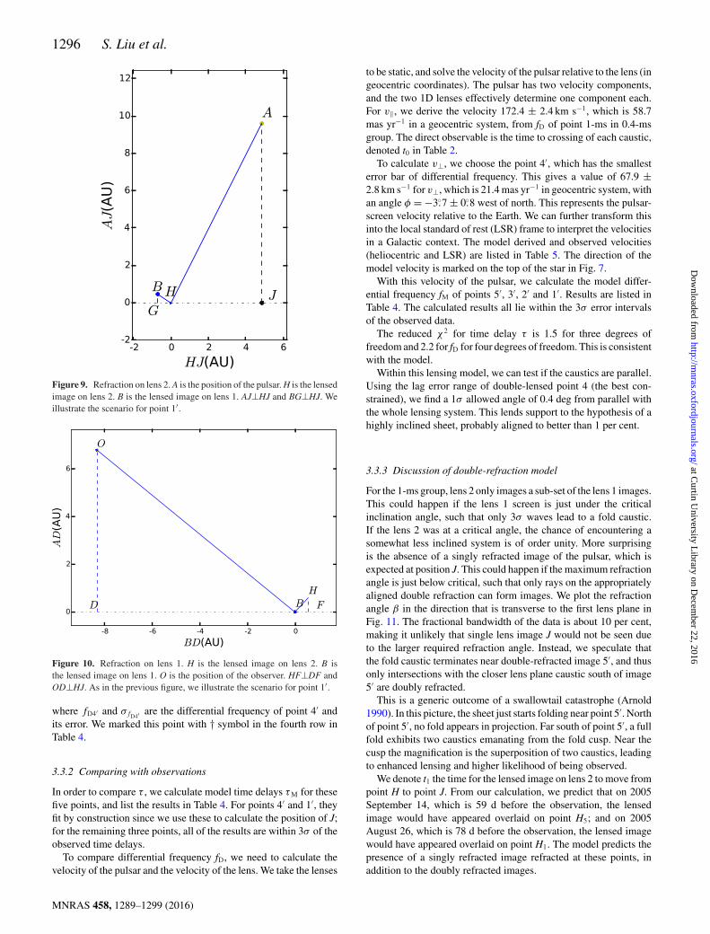
Figure 9. Refraction on lens 2. A is the position of the pulsar. H is the lensedimage on lens 2. B is the lensed image on lens 1. AJ⊥HJ and BG⊥HJ. Weillustrate the scenario for point 1′.

Figure 10. Refraction on lens 1. H is the lensed image on lens 2. B isthe lensed image on lens 1. O is the position of the observer. HF⊥DF andOD⊥HJ. As in the previous figure, we illustrate the scenario for point 1′.

where fD4′ and σfD4′ are the differential frequency of point 4′ andits error. We marked this point with † symbol in the fourth row inTable 4.

3.3.2 Comparing with observations

In order to compare τ , we calculate model time delays τM for thesefive points, and list the results in Table 4. For points 4′ and 1′, theyfit by construction since we use these to calculate the position of J;for the remaining three points, all of the results are within 3σ of theobserved time delays.

To compare differential frequency fD, we need to calculate thevelocity of the pulsar and the velocity of the lens. We take the lenses

to be static, and solve the velocity of the pulsar relative to the lens (ingeocentric coordinates). The pulsar has two velocity components,and the two 1D lenses effectively determine one component each.For v‖, we derive the velocity 172.4 ± 2.4 km s−1, which is 58.7mas yr−1 in a geocentric system, from fD of point 1-ms in 0.4-msgroup. The direct observable is the time to crossing of each caustic,denoted t0 in Table 2.

To calculate v⊥, we choose the point 4′, which has the smallesterror bar of differential frequency. This gives a value of 67.9 ±2.8 km s−1 for v⊥, which is 21.4 mas yr−1 in geocentric system, withan angle φ = −3.◦7 ± 0.◦8 west of north. This represents the pulsar-screen velocity relative to the Earth. We can further transform thisinto the local standard of rest (LSR) frame to interpret the velocitiesin a Galactic context. The model derived and observed velocities(heliocentric and LSR) are listed in Table 5. The direction of themodel velocity is marked on the top of the star in Fig. 7.

With this velocity of the pulsar, we calculate the model differ-ential frequency fM of points 5′, 3′, 2′ and 1′. Results are listed inTable 4. The calculated results all lie within the 3σ error intervalsof the observed data.

The reduced χ2 for time delay τ is 1.5 for three degrees offreedom and 2.2 for fD for four degrees of freedom. This is consistentwith the model.

Within this lensing model, we can test if the caustics are parallel.Using the lag error range of double-lensed point 4 (the best con-strained), we find a 1σ allowed angle of 0.4 deg from parallel withthe whole lensing system. This lends support to the hypothesis of ahighly inclined sheet, probably aligned to better than 1 per cent.

3.3.3 Discussion of double-refraction model

For the 1-ms group, lens 2 only images a sub-set of the lens 1 images.This could happen if the lens 1 screen is just under the criticalinclination angle, such that only 3σ waves lead to a fold caustic.If the lens 2 was at a critical angle, the chance of encountering asomewhat less inclined system is of order unity. More surprisingis the absence of a singly refracted image of the pulsar, which isexpected at position J. This could happen if the maximum refractionangle is just below critical, such that only rays on the appropriatelyaligned double refraction can form images. We plot the refractionangle β in the direction that is transverse to the first lens plane inFig. 11. The fractional bandwidth of the data is about 10 per cent,making it unlikely that single lens image J would not be seen dueto the larger required refraction angle. Instead, we speculate thatthe fold caustic terminates near double-refracted image 5′, and thusonly intersections with the closer lens plane caustic south of image5′ are doubly refracted.

This is a generic outcome of a swallowtail catastrophe (Arnold1990). In this picture, the sheet just starts folding near point 5′. Northof point 5′, no fold appears in projection. Far south of point 5′, a fullfold exhibits two caustics emanating from the fold cusp. Near thecusp the magnification is the superposition of two caustics, leadingto enhanced lensing and higher likelihood of being observed.

We denote t1 the time for the lensed image on lens 2 to move frompoint H to point J. From our calculation, we predict that on 2005September 14, which is 59 d before the observation, the lensedimage would have appeared overlaid on point H5; and on 2005August 26, which is 78 d before the observation, the lensed imagewould have appeared overlaid on point H1. The model predicts thepresence of a singly refracted image refracted at these points, inaddition to the doubly refracted images.

MNRAS 458, 1289–1299 (2016)

at Curtin U


ecember 22, 2016


Dow

nloaded from



Table 5. Summary of velocities in the double-refraction model. The velocities listed in equatorial coordinates are the relative velocity in heliocentric system,while the velocities in Galactic coordinates are the relative velocities in LSR. μα∗ = �αcos (δ)/t and μl∗ = �lcos (b)/t, for which we move the centre positionfrom (�α, �δ) or (l, b) to (0,0). vl∗ and vb are the linear velocities relative to the LSR. The screen is only moving slowly (∼21 km s−1). Ellipses reflect theunobserved and frame-dependent parameters.

Parameter μα∗(mas yr−1) μδ(mas yr−1) μl∗(mas yr−1) μb (mas yr−1) vl∗ (km s−1) vb (km s−1)

Model pulsar-screen velocity −5.30 ± 1.11 61.97 ± 1.11 −56.45 22.23 – –VLBI pulsar proper motion 2.16 ± 0.19 51.64 ± 0.13 −46.69 28.02 −137.24 82.34

Screen motion – – 9.76 5.79 18.00 10.68

Figure 11. Deflection angle β = π− ∠AHB on lens 2. Point J denotes theexpected position to form a single refraction image, which is not observed.The small change in angle relative to the observed images precludes afinite refraction cut-off, since the data spans 10 per cent bandwidth, with a20 per cent change in refractive strength. We propose a swallowtail causticas the likely origin for the termination of the second lens sheet.

The generic flux of a lensed image is the ratio of the lens trans-verse size to maximum impact parameter (Pen & King 2012). Nearthe caustic, the lensed flux can become very high. The 1-ms group isabout a factor of 4 fainter than the 0.4-ms group. The high flux of thesecond caustic suggests it to be relatively wide, perhaps a fraction ofan au. Due to the odd image theorem, one generically expects twodistinct sets of double-lensed arcs. We only see one (generically theouter one), which places an upper bound on the brightness of theinner image. In a divergent lens (Clegg et al. 1998), the inner imageis generically much fainter, so perhaps this is not surprising. For aconvergent Gaussian lens, the two images are of similar brightness,but a more cuspy profile will also result in a faint inner image. Ingravitational lensing, the odd image theorem is rarely seen to hold,which is generally thought to be due to one lens being very faint.

One can try to estimate the chance of accidental agreement be-tween model and data. We show the data visually in Fig. 12.

To estimate where points might lie accidentally, we conserva-tively compare the area of the error regions to the area boundedby the parabola and the data points, as shown by dotted lines. Thisresults in about 10−3, suggesting that the model is unlikely to be anaccidental fit.

It might be a good supplementary study to conduct a multiscreensimulation that provides ray tracing through a large number ofinclined sheets. By adjusting the parameters, we can test the pos-sibility of multirefractions. However, this is obviously beyond thescope of the current paper.

Figure 12. Model comparison. Points with subscripts are derived from thedouble-refraction model, see Table 4. Rectangles mark the 1σ error region.Points 1′ (only for τ ) and 4′ are used to fit the model, and thus do not havean error region. The rectangles cover 10−3 of the area in the dotted regionbounded by the parabolic arc and the data points. We interpret this preciseagreement between model and data is unlikely to be a random coincidence.

3.4 Distance degeneracies

With two lens screens, the number of observables increases: inprinciple one could observe both single refraction delays andangular positions, as well as the double-refraction delays andangular positions. Three distances are unknown, equal to the num-ber of observables. Unfortunately, these measurements are de-generate, which can be seen as follows. From the two screensi = 1, 2, the two single refraction effective distance observablesare Die ≡ 2cτi/θ

2i = D2

i (1/Di + 1/Dpi). A third observable ef-fective distance is that of screen 2 using screen 1 as a lens,D21e = D2

1(1/D1 + 1/D21), within the triangle that is formed bylens 1, lens 2, and the observer. That is also algebraically deriv-able from the first two relations: D21e = D1eD2e/(D2e − D1e). Weillustrate the light path in Fig. 13.

In this archival data set, the direct single lens from the furtherplane at position J is missing. It would have been visible 59 d earlier.The difference in time delays to image J and the double-refractionimages would allow a direct determination of the effective distanceto lens plane 2. Because ∠ DAJ is close to 90◦ angle, the effectwould be about a factor of 10 ill conditioned. With sufficientlyprecise VLBI imaging one could distinguish if the doubly refractedimages are at position B (if lens 1 is closer to the observer) orposition H (if lens 2 is closer to the observer). As described above,we interpret the effective distances to place screen 2 further away.

MNRAS 458, 1289–1299 (2016)

at Curtin U


ecember 22, 2016


Dow

nloaded from


1298 S. Liu et al.

Figure 13. Illustration of double-refraction degeneracy. As in Fig. 5, all observables are identical for both the prime and unprimed geometries, including allpairwise delays and angular positions. This degeneracy also holds in three dimensions.

4 D ISCUSSIONS

4.1 Interpretation

The relative motion between pulsar and lens is directly measuredby the differential frequency, and is not sensitive to details of thismodel. B10 derived similar motions. This motion is in broad agree-ment with direct VLBI proper motion measurement, requiring thelens to be moving slowly compared to the pulsar proper motion orthe LSR. The lens is ∼200 pc above the Galactic disc. Matter caneither be in pressure equilibrium, or in free fall, or some combi-nation thereof. In free fall, one expects substantial motions. Thesedata rule out retrograde or radially Galactic orbits and indicate thatthe lens is corotating with the Galaxy. In pressure equilibrium, gasrotates slower as its pressure scaleheight increases, which appearsconsistent with the observed slightly slower than corotating motion.The modest lens velocities also appear consistent with the generalmotion of the interstellar medium (ISM), perhaps driven by Galacticfountains (Shapiro & Field 1976) at these latitudes above the disc. Inthe inclined sheet model, the waves move at Alfvenic speed, but dueto the high inclination, they will move less than one percent of thisspeed in projection on the sky, and thus be completely negligiblecompared to other sources of motion.

Alternative models, for example, evaporating clouds (Walker &Wardle 1998) or strange matter (Perez-Garcıa, Silk & Pen 2013), donot make clear predictions. One would expect higher proper motionsfrom these freely orbiting sources, and larger future scintillationsamples may constrain these models.

Inclining one sheet randomly to better than 1 per cent requires oforder 104 randomly placed sheets, i.e. many per parsec. This sheetextends for ∼ 10 au in projection, corresponding to a physical scalegreater than 1000 au. These two numbers roughly agree, leading toa physical picture of magnetic domain boundaries every ∼0.1 pc.B0834+06 had noted arcs for multiple years, perhaps suggestingthis dominant lens plane is larger than typical. One might expect toreach the end of the sheet within decades.

A generic prediction of the inclined sheets model is a changein rotation measure (RM) across the scattering length. Over 1000au, one might expect a typical RM change of 10−3 rad m−2. Atlow frequencies, for example in LOFAR1 or GMRT,2 the size ofthe scattering screen extends another order of magnitude in angularsize, and the RM in different lensed images are different, increasingto ∼0.01, which is plausibly measurable. Even for an unpolarizedsource, the left and right circularly polarized (LCP, RCP) dynamicspectra will be slightly different. Usually a SS is formed by Fouriertransforming the dynamic spectrum and multiplying by its complexconjugate. To measure the RM, one multiplies the Fourier transform

1 http://www.lofar.org/2 http://gmrt.ncra.tifr.res.in/

of the LCP dynamic spectrum by the complex conjugate of theRCP Fourier transform. This will display a phase gradient alongthe Doppler frequency axis. In the SS, each pixel is the sum ofcorrelations of pairs of scattering points with corresponding lagand Doppler velocity. The velocity is typically linear in the pairseparation, which is also the case for differential RM. This statisticis analogous to the cross gate SS as applied in Pen et al. (2014).

4.2 Possible improvements

We discuss several strategies which can improve on the solutionaccuracy. The single biggest improvement would be to monitorthe speckle pattern over several months, as the pulsar crosses eachindividual lens, including both lensing systems. This allows a directcomparison of single-refraction to double-refraction arclets.

Angular resolution can be improved using longer baselines, forexample adding a GMRT–GBT baseline doubles the resolution.Observing at multiple frequencies over a longer period allows for amore precise measurement: when the pulsar is between two lenses,the refraction angle β is small, and one expects to see the lensingat higher frequency, where the resolution is higher, and distancesbetween lens positions can be measured to much higher accuracy.

Holographic techniques (Walker et al. 2008; Pen et al. 2014)may be able to measure delays, fringe rates, and VLBI positionssubstantially more accurately. Combining these techniques, the in-terstellar lensing could conceivably achieve distance measurementsan order of magnitude better than the current published effectivedistance errors. This could bring most pulsar timing array targetsinto the coherent timing regime, enabling arc minute localization ofgravitational wave sources, lifting any potential source confusion.

Ultimately, the precision of the lensing results would be limitedby the fidelity of the lensing model. In the inclined sheet model,the images move along fold caustics. The straightness of thesecaustics depends on the inclination angle, which in turn depends onthe amplitude of the surface waves. This analysis indicates a highdegree of inclination, and thus high fidelity for geometric pulsarstudies.

5 C O N C L U S I O N S

We have applied the inclined sheet model (Pen & Levin 2014) toarchival apex data of PSR B0834+06. The data are well fitted bytwo linear lensing screens, with nearly planar geometry. The secondscreen provides a precision test with 10 observables (five time de-lays and five differential frequencies) and three free parameters (themarked points in Table 4). On each of the seven points, the modelfits the data to ∼ per cent accuracy. This natural consequence of verysmooth reconnection sheets is an unlikely outcome of ISM turbu-lence. These results, if extrapolated to multi-epoch observations ofbinary systems, might result in accurate distance determinations and

MNRAS 458, 1289–1299 (2016)

at Curtin U


ecember 22, 2016


Dow

nloaded from

http://www.lofar.org/

http://gmrt.ncra.tifr.res.in/



opportunities for removing scattering induced timing errors. Thisapproach also opens the window to measuring precise transversemotions of the ionized ISM outside the Galactic plane.

AC K N OW L E D G E M E N T S

We thank NSERC for support. We acknowledge helpful discussionswith Peter Goldreich and M. van Kerkwijk. We thank MichaelWilliams for photography help. SL thanks Robert Main and JDEmberson for helpful discussions on improving the expression ofthe content. JPM acknowledges support through the Australian Re-search Council grant DP140104114. The Dunlap Institute is fundedthrough an endowment established by the David Dunlap family andthe University of Toronto. The National Radio Astronomy Observa-tory is a facility of the National Science Foundation operated undercooperative agreement by Associated Universities, Inc.

R E F E R E N C E S

Arnold V. I., 1990, Singularities of Caustics and Wave Fronts. Springer-Verlag, Netherlands

Boyle L., Pen U.-L., 2012, Phys. Rev. D, 86, 124028Braithwaite J., 2015, MNRAS, 450, 3201Brisken W. F., Macquart J.-P., Gao J. J., Rickett B. J., Coles W. A., Deller

A. T., Tingay S. J., West C. J., 2010, ApJ, 708, 232 (B10)Clegg A. W., Fey A. L., Lazio T. J. W., 1998, ApJ, 496, 253Cordes J. M., Rickett B. J., Stinebring D. R., Coles W. A., 2006, ApJ, 637,

346

Deller A. T. et al., 2012, ApJ, 756, L25Deller A. T., Boyles J., Lorimer D. R., Kaspi V. M., McLaughlin M. A.,

Ransom S., Stairs I. H., Stovall K., 2013, ApJ, 770, 145Efron B., Tibshirani R., 1991, Science, 253, 390Goldreich P., Sridhar S., 2006, ApJ, 640, L159Hill A. S., Stinebring D. R., Barnor H. A., Berwick D. E., Webber A. B.,

2003, ApJ, 599, 457Kramer M. et al., 2006, Science, 314, 97Longuet-Higgins M. S., 1960, J. Opt. Soc. Am., 50, 845Lorimer D. R., Kramer M., 2012, Handbook of Pulsar Astronomy. Cam-

bridge Univ. Press, CambridgePen U.-L., King L., 2012, MNRAS, 421, L132Pen U.-L., Levin Y., 2014, MNRAS, 442, 3338Pen U.-L., Macquart J.-P., Deller A. T., Brisken W., 2014, MNRAS, 440,

L36Perez-Garcıa M. A., Silk J., Pen U.-L., 2013, Phys. Lett. B, 727, 357Shapiro P. R., Field G. B., 1976, ApJ, 205, 762Stinebring D. R., McLaughlin M. A., Cordes J. M., Becker K. M., Goodman

J. E. E., Kramer M. A., Sheckard J. L., Smith C. T., 2001, ApJ, 549, L97Walker M., Wardle M., 1998, ApJ, 498, L125Walker M., Melrose D., Stinebring D., Zhang C., 2004, MNRAS, 354, 43Walker M. A., Koopmans L. V. E., Stinebring D. R., van Straten W., 2008,

MNRAS, 388, 1214

This paper has been typeset from a TEX/LATEX file prepared by the author.

MNRAS 458, 1289–1299 (2016)

at Curtin U


ecember 22, 2016


Dow

nloaded from


pulsar lensing geometry

Documents