The Geometry of Gravitational Lensing:

Magnification Relations, Observables, and Kerr

Black Holes

by

Amir Babak Aazami

Department of MathematicsDuke University

Date:

Approved:

Arlie O. Petters, Advisor

Hubert L. Bray

Charles R. Keeton

Marcus C. Werner

Dissertation submitted in partial fulfillment of the requirements for the degree ofDoctor of Philosophy in the Department of Mathematics

in the Graduate School of Duke University2011

Abstract(Mathematics)

The Geometry of Gravitational Lensing: Magnification

Relations, Observables, and Kerr Black Holes

by

Amir Babak Aazami

Department of MathematicsDuke University

Date:

Approved:

Arlie O. Petters, Advisor

Hubert L. Bray

Charles R. Keeton

Marcus C. Werner

An abstract of a dissertation submitted in partial fulfillment of the requirements forthe degree of Doctor of Philosophy in the Department of Mathematics

in the Graduate School of Duke University2011

Copyright © 2011 by Amir Babak Aazami in Chapters 1 and 6Chapters 2 – 5 © held by the American Institute of Physics

Abstract

Gravitational lensing is the study of the bending of light by gravity. In such a

scenario, light rays from a background star are deflected as they pass by a foreground

galaxy (the “lens”). If the lens is massive enough, then multiple copies of the light

source, called “lensed images,” are produced. These are magnified or demagnified

relative to the light source that gave rise to them. Under certain conditions their

sum is an invariant: it does not depend on where these lensed images are in the sky

or even the details of the lens mass producing them. One of the main results of this

thesis is the discovery of a new, infinite family of such invariants, going well beyond

the previously known class of two. The application of this result to the search for

dark matter in galaxies is also discussed.

The second main result of this thesis is a new general lens equation and magnifi-

cation formula governing lensing by Kerr black holes, for source and observer lying

in the asymptotically flat region of the spacetime. The reason for deriving these

quantities is because the standard gravitational lensing framework assumes that the

gravitational field of the lens is weak, so that a Newtonian potential can be applied

to model it. This assumption obviously breaks down in the vicinity of a black hole,

where the gravity is immense. As a result, one has to go directly to the Kerr metric

and its associated geometric quantities, and derive an equation for light bending

from first principles. This equation is then solved perturbatively to obtain lensing

observables (image position, magnification, time delay) beyond leading order.

iv

to my father, mother, and sister, with love

v

Contents

Abstract iv

List of Tables ix

List of Figures x

Acknowledgements xi

1 Introduction 1

1.1 Magnification Relations . . . . . . . . . . . . . . . . . . . . . . . . . . 1

1.2 Lensing by Kerr Black Holes . . . . . . . . . . . . . . . . . . . . . . . 6

1.3 Declaration . . . . . . . . . . . . . . . . . . . . . . . . . . . . . . . . 7

2 Magnification Theorem for Higher-Order Caustic Singularities 10

2.1 Introduction . . . . . . . . . . . . . . . . . . . . . . . . . . . . . . . . 10

2.2 Basic Concepts . . . . . . . . . . . . . . . . . . . . . . . . . . . . . . 12

2.2.1 Lensing Theory . . . . . . . . . . . . . . . . . . . . . . . . . . 12

2.2.2 Higher-Order Caustic Singularities in Lensing . . . . . . . . . 14

2.2.3 Caustic Singularities of the A,D,E family . . . . . . . . . . . 16

2.3 The Magnification Theorem . . . . . . . . . . . . . . . . . . . . . . . 18

2.4 Applications . . . . . . . . . . . . . . . . . . . . . . . . . . . . . . . . 19

3 Proof of Magnification Theorem 28

3.1 An Algebraic Proposition . . . . . . . . . . . . . . . . . . . . . . . . . 28

3.1.1 A Recursive Relation for Coefficients of Coset Polynomials . . 28

vi

3.1.2 Proof of Proposition 2 . . . . . . . . . . . . . . . . . . . . . . 32

3.2 Algebraic Proof of Magnification Theorem . . . . . . . . . . . . . . . 37

3.3 Orbifolds and Multi-Dimensional Residues . . . . . . . . . . . . . . . 42

3.3.1 Weighted Projective Space as a Compact Orbifold . . . . . . . 43

3.3.2 Multi-Dimensional Residue Theorem on Compact Orbifolds . 47

3.4 Geometric Proof of Magnification Theorem . . . . . . . . . . . . . . . 51

3.4.1 Singularities of Type An . . . . . . . . . . . . . . . . . . . . . 51

3.4.2 Singularities of Type Dn . . . . . . . . . . . . . . . . . . . . . 52

3.4.3 Singularities of Type En . . . . . . . . . . . . . . . . . . . . . 53

3.4.4 Quantitative Forms for the Elliptic and Hyperbolic Umbilics . 54

4 A Lens Equation for Equatorial Kerr Black Hole Lensing 56

4.1 Introduction . . . . . . . . . . . . . . . . . . . . . . . . . . . . . . . . 56

4.2 General Lens Equation with Displacement . . . . . . . . . . . . . . . 57

4.2.1 Angular Coordinates on the Observer’s Sky . . . . . . . . . . 57

4.2.2 General Lens Equation via Asymptotically Flat Geometry . . 59

4.2.3 General Magnification Formula . . . . . . . . . . . . . . . . . 63

4.3 Lens Equation for Kerr Black Holes . . . . . . . . . . . . . . . . . . . 64

4.3.1 Kerr Metric . . . . . . . . . . . . . . . . . . . . . . . . . . . . 64

4.3.2 Lens Equation for an Equatorial Observer . . . . . . . . . . . 66

4.3.3 Schwarzschild Case . . . . . . . . . . . . . . . . . . . . . . . . 67

4.4 Exact Kerr Null Geodesics for Equatorial Observers . . . . . . . . . . 67

4.4.1 Equations of Motion for Null Geodesics . . . . . . . . . . . . . 68

4.4.2 Exact Lens Equation for Equatorial Observers . . . . . . . . . 69

5 Quasi-Equatorial Lensing Observables 73

5.1 Introduction . . . . . . . . . . . . . . . . . . . . . . . . . . . . . . . . 73

vii

5.2 Definitions and Assumptions . . . . . . . . . . . . . . . . . . . . . . . 73

5.3 Quasi-Equatorial Kerr Light Bending . . . . . . . . . . . . . . . . . . 75

5.4 Observable Properties of Lensed Images . . . . . . . . . . . . . . . . 78

5.4.1 Quasi-Equatorial Lens Equation . . . . . . . . . . . . . . . . . 78

5.4.2 Image Positions . . . . . . . . . . . . . . . . . . . . . . . . . . 81

5.4.3 Magnifications . . . . . . . . . . . . . . . . . . . . . . . . . . . 84

5.4.4 Critical and Caustic Points . . . . . . . . . . . . . . . . . . . . 86

5.4.5 Total Magnification and Centroid . . . . . . . . . . . . . . . . 88

5.4.6 Time Delay . . . . . . . . . . . . . . . . . . . . . . . . . . . . 89

5.5 Remarks on Lensing Observables . . . . . . . . . . . . . . . . . . . . 90

5.6 Transformation from Sky Coordinates to Boyer-Lindquist Coordinates 92

5.7 Quasi-Equatorial Kerr Bending Angle . . . . . . . . . . . . . . . . . . 94

5.7.1 Equations of Motion for Quasi-Equatorial Null Geodesics . . . 94

5.7.2 Horizontal Light Bending Angle . . . . . . . . . . . . . . . . . 97

5.7.3 Vertical Bending Angle . . . . . . . . . . . . . . . . . . . . . . 102

5.8 Quasi-Equatorial Time Delay . . . . . . . . . . . . . . . . . . . . . . 107

6 Future Goals 110

Bibliography 111

Biography 116

viii

List of Tables

2.1 Local Form of Lensing Map Near Elliptic and Hyperbolic Umbilics . . 15

2.2 Arnold’s A,D,E Classification of Caustic Singularities . . . . . . . . 17

2.3 Rh.u. and Rfold for an SIE with Source Approaching a Fold . . . . . . 24

2.4 Rh.u. and Rcusp for an SIE with Source Approaching a Cusp . . . . . . 25

ix

List of Figures

1.1 Observed Lensed Images in Gravitational Lensing . . . . . . . . . . . 2

1.2 Schematic of Gravitational Lensing . . . . . . . . . . . . . . . . . . . 3

2.1 Image Configurations for an SIE and Hyperbolic Umbilic Lensing Map 27

4.1 Angles on the Observer’s Sky . . . . . . . . . . . . . . . . . . . . . . 58

4.2 “Displacement” in Lensing . . . . . . . . . . . . . . . . . . . . . . . . 59

4.3 A Detailed Diagram of Lensing Geometry . . . . . . . . . . . . . . . 61

4.4 Boyer-Lindquist Coordinates Centered on Kerr Black Hole . . . . . . 64

5.1 First- and Second- order Angular Image Correction Terms . . . . . . 84

5.2 Alternate Coordinates Centered on Kerr Black Hole . . . . . . . . . . 93

x

Acknowledgements

From Yale, I would like to thank Richard Easther for his early support, and especially

Priyamvada Natarajan; without her help this thesis would not have been possible.

I also thank Hubert Bray, Charles Keeton, and Jeffrey Rabin for being fantastic

collaborators, as well as Marcus Werner for stimulating discussions. Most especially,

however, I thank my adviser and mentor Arlie Petters, from whom I have learned so

much.

xi

1

Introduction

Gravitational lensing is the study of the bending of light by gravity. In such a

scenario, light rays from a background star are deflected as they pass by a foreground

galaxy (the “lens”). This effect was predicted by Einstein in 1911 as a consequence of

his general theory of relativity, and first observed by Eddington in 1919. The field is

now a vibrant area of research in astronomy, physics, and mathematical physics (see,

e.g., Schneider et al. (1992); Petters et al. (2001); Petters (2010)). The phenomenon

of light bending is an extraordinary one: if the lens is massive enough, then multiple

copies of the light source, called “lensed images,” are produced; see Fig. 1.1 for

examples.

1.1 Magnification Relations

Chapters 2 and 3 of this dissertation focus on an important aspect of this phe-

nomenon: lensed images are magnified or demagnified relative to the light source

that gave rise to them. Formally, the magnification is a ratio of solid angles, sub-

tended by the lensed image and source. Surprisingly, under certain conditions the

sum of the magnifications of lensed images is an invariant: it does not depend on

1

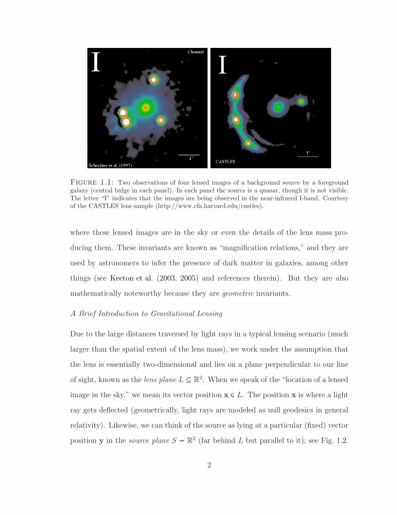
Figure 1.1: Two observations of four lensed images of a background source by a foregroundgalaxy (central bulge in each panel). In each panel the source is a quasar, though it is not visible.The letter “I” indicates that the images are being observed in the near-infrared I-band. Courtesyof the CASTLES lens sample (http://www.cfa.harvard.edu/castles).

where these lensed images are in the sky or even the details of the lens mass pro-

ducing them. These invariants are known as “magnification relations,” and they are

used by astronomers to infer the presence of dark matter in galaxies, among other

things (see Keeton et al. (2003, 2005) and references therein). But they are also

mathematically noteworthy because they are geometric invariants.

A Brief Introduction to Gravitational Lensing

Due to the large distances traversed by light rays in a typical lensing scenario (much

larger than the spatial extent of the lens mass), we work under the assumption that

the lens is essentially two-dimensional and lies on a plane perpendicular to our line

of sight, known as the lens plane L R2. When we speak of the “location of a lensed

image in the sky,” we mean its vector position x P L. The position x is where a light

ray gets deflected (geometrically, light rays are modeled as null geodesics in general

relativity). Likewise, we can think of the source as lying at a particular (fixed) vector

position y in the source plane S R2 (far behind L but parallel to it); see Fig. 1.2.

2

Figure 1.2: Schematic of gravitational lensing. A light ray emitted from a source at y P S isdeflected by an angle α at the lens plane at x P L. An observer thus sees (one copy of) the sourceat x P L. Courtesy of Petters (2010).

With these quantities in hand, one can then ask: “If a light ray is deflected by the

lens and then reaches us, how much longer is its arrival time compared to a light ray

that would have directly reached us in the absence of a lens?” We quantify this “time

delay” by the time delay function, a smooth real-valued function Ty : L ÝÑ R. This

function actually contains within it the core of gravitational lensing theory. We now

apply Fermat’s principle of “least time,” which says that light rays emitted from a

source that reach us are realized as critical points of the time delay function (and so

the mathematical origins of gravitational lensing theory ultimately lie in symplectic

geometry). In other words, a lensed image of a light source at y is a critical point

of Ty, i.e., a solution x P L of the equation pgradTyqpxq 0, where the gradient is

taken with respect to x. With this information in hand, we can now geometrically

define the notion of magnification: the signed magnification of a lensed image x P Lof a light source at y P S is

µpx;yq 1

Gausspx, Typxqq ,where Gausspx, Typxqq is the Gaussian curvature of the graph of Ty at the criti-

cal point px, Typxqq. This definition makes clear why magnification relations are

3

geometric invariants. (Though not obvious, it is equivalent to the definition given

in terms of solid angles above.) But it also begs the question: What happens if

Gausspx, Typxqq 0? Any y P S giving rise to such an x is called a caustic point.

The set of all caustic points typically forms smooth curves, but could also include

isolated points. Since we do not expect to see lensed images with infinite magnifica-

tion in the sky (mathematically, caustics form a set of measure zero), the important

question then becomes whether a source lies near a caustic. If it does, then very in-

teresting things happen, as we shall see below. Indeed, in Fig. 1.1 above, the source

in each case lies near a caustic, and this accounts for the particular configuration the

four lensed images assume (in the left panel, notice that two images lie very close

together, while in the right panel there is a triplet of images positioned away from

the fourth). To better understand this relation between caustics and the observed

positions of lensed images, one must delve into the mathematical subject known as

singularity theory, which is the systematic analysis of the critical point and caustic

structure of families of smooth functions.

A Brief Introduction to Singularity Theory

In one of the major achievements in singularity theory, Vladimir Arnold in 1973

classified the possible types of stable caustics that can occur (Arnold’s classifica-

tion incorporated and went beyond an earlier classification by Rene Thom in the

1960s). Specifically, Arnold classified all stable simple Lagrangian map-germs of

n-dimensional Lagrangian submanifolds by their generating family Fc,y (these are

analogous to the time delay function Ty); see Arnold (1973). In the process, he

found a remarkable connection between his classification and the Coxeter-Dynkin

diagrams of the simple Lie algebras of types An pn ¥ 2q, Dn pn ¥ 4q, E6, E7, E8. This

is now known as Arnold’s A,D,E classification of caustic singularities; see Table 2.2

of Chapter 2.

4

The time delay function Typxq can be viewed as a two-parameter family of func-

tions with parameter the light source position y P S. In this two-dimensional setting,

it can be shown that a “generic” time delay function will give rise to only two types

of “generic” caustic points: folds and cusps (“generic” is here used in a well-defined

sense; ultimately, we are living in the Whitney C8-topology in a given space of map-

pings). Folds are arcs on the source plane that abut isolated cusp points. These

are the simplest examples of caustic singularities in Arnold’s classification. Now,

let Tc,ypxq denote a family of time delay functions parametrized by the source po-

sition y and c P R. (In the context of gravitational lensing, the parameter c may

denote the core radius of the galaxy acting as lens, or the redshift of the source,

or some other physical input.) The three-parameter family Tc,ypxq gives rise to a

more sophisticated and higher-order caustic structure. Varying c causes the caustic

curves in the light source plane S to evolve with c. This traces out a caustic surface

in the three-dimensional space R R2 tpc,yqu. The source plane S would then

be a particular “c-slice” of this caustic surface. Beyond folds and cusps, these sur-

faces are classified into three generic types, namely, swallowtails, elliptic umbilics,

and hyperbolic umbilics. And so on; more and more parameters give rise to higher-

and higher-order caustic surfaces, with ever-more beautiful (and strange) shapes. In

Arnold’s classification, it turns out that the fold, cusp, swallowtail, and umbilics are

classified by the Dynkin diagrams A2, A3, A4, and D4, respectively.

Having said this, there is no reason to restrict the notion of magnification to time-

delay functions alone. Indeed, consider a smooth n-parameter generating family

Fc,ypxq of functions on an open subset of R2 that exhibits a caustic singularity

classified by Arnold’s A,D,E classification. We can then define the magnification

of Fc,ypxq at a critical point x in exactly the same way as we did for time-delay

5

functions, namely, as

Mpx;yq 1

Gausspx, Fc,ypxqq ,where we use the symbol M to distinguish magnification in the generic sense from

its use in gravitational lensing. Armed with this definition, we can now inquire

whether we can uncover “magnification relations” for any of the caustic singularities

in Arnold’s family. The surprising answer is that all of them exhibit a magnification

relation of the following form:

n

i1

Mpxi;yq 0 , (1.1)

where xi are the n critical points of a particular generating family Fc,ypxq with y

fixed (in fact its number of critical points is equal to its index as a Dynkin diagram;

i.e., of type An pn ¥ 2q, Dn pn ¥ 4q, E6, E7, E8). The key result in Chapters 2 and 3 is

Theorem 1, which establishes eqn. (1.1) and provides a geometric explanation for its

existence. We will see that this geometric explanation relies upon multi-dimensional

residue techniques and the geometry of orbifolds.

1.2 Lensing by Kerr Black Holes

Chapters 4 and 5 develop a unified, analytic framework for gravitational lensing

by Kerr black holes. These are rotating black holes, the metrics for which were

discovered by Roy Kerr in 1963. Chapter 4 presents a new, general lens equation

and magnification formula governing lensing by an arbitrary thin deflector. Our lens

equation assumes that the source and observer are in the asymptotically flat region.

Furthermore, whereas in all lensing scenarios it is assumed that the bending of the

light ray takes place on the plane perpendicular to the line of sight containing the

lens (as in Fig. 1.2 above), that assumption is not made here. Thus the lens equation

6

presented in Chapter 4 takes into account the displacement that occurs when the

light ray’s tangent lines at the source and observer do not meet on the lens plane.

Next, restricting to the case when the thin deflector is a Kerr black hole, an explicit

expression is given for the displacement when the observer is in the equatorial plane

of the Kerr black hole, as well as for the case of spherical symmetry. The reason

for deriving these quantities is because the standard gravitational lensing framework

assumes that the gravitational field of the lens is weak, so that a Newtonian potential

can be applied to model it. This assumption obviously breaks down in the vicinity

of a black hole, where the gravity is immense. As a result, one has to go directly to

the Kerr metric and its associated geometric invariants, and derive an equation for

light bending from first principles. This is the goal of Chapter 4.

Chapter 5 then explores this lens equation; specifically, it develops an analytical

theory of quasi-equatorial lensing by Kerr black holes. In this setting the general lens

equation (with displacement) is solved perturbatively, going beyond weak-deflection

Kerr lensing to second order in the expansion parameter ε, which is the ratio of

the angular gravitational radius to the angular Einstein radius. New formulas and

results are obtained for the bending angle, image positions, image magnifications,

total unsigned magnification, centroid, and time delay, all to second order in ε and

including the displacement. For all lensing observables it is shown that the displace-

ment begins to appear only at second order in ε. When there is no spin, new results

are obtained on the lensing observables for Schwarzschild lensing with displacement.

1.3 Declaration

This dissertation is the result of my work under the guidance of my adviser Prof. Arlie

Petters and two collaborators, Prof. Jeffrey Rabin and Prof. Charles Keeton. The

following chapters are based on, or have been excerpted/reproduced from, articles

that have either been published or are currently under review for publication:

7

Chapter 2:

• Aazami, A. B., Petters, A. O., A universal magnification theorem for higher-

order caustic singularities, J. Math. Phys. 50, 032501, Copyright 2009, The

American Institute of Physics.

• Aazami, A. B., Petters, A. O., A universal magnification theorem. III. Caustics

beyond codimension five, J. Math. Phys. 51, 023503, Copyright 2010, The

American Institute of Physics.

This chapter may be downloaded for personal use only.

Chapter 3:

• Aazami, A. B., Petters, A. O., A universal magnification theorem II. Generic

caustics up to codimension five, J. Math. Phys. 50, 082501, Copyright 2009,

The American Institute of Physics.

• Aazami, A. B., Petters, A. O., A universal magnification theorem. III. Caustics

beyond codimension five, J. Math. Phys. 51, 023503, Copyright 2010, The

American Institute of Physics.

• Aazami, A. B., Rabin, J. M., and Petters, A. O., Orbifolds, the A,D,E family

of caustic singularities, and gravitational lensing, J. Math. Phys. 52, 022501,

Copyright 2011, The American Institute of Physics.

This chapter may be downloaded for personal use only.

Chapter 4:

• Aazami, A. B., Keeton, C. R., and Petters, A. O., Lensing by Kerr black holes.

I. General lens equation and magnification formula, submitted to J. Math.

Phys., Copyright 2011, The American Institute of Physics.

8

This chapter may be downloaded for personal use only.

Chapter 5:

• Aazami, A. B., Keeton, C. R., and Petters, A. O., Lensing by Kerr black holes.

II. Analytical study of quasi-equatorial lensing observables, submitted to J.

Math. Phys., Copyright 2011, The American Institute of Physics.

This chapter may be downloaded for personal use only.

9

2

Magnification Theorem for Higher-Order Caustic

Singularities

2.1 Introduction

One of the key signatures of gravitational lensing is the occurrence of multiple im-

ages of lensed sources. The magnifications of the images in turn are also known to

obey certain relations. One of the simplest examples of a magnification relation is

that due to a single point-mass lens, where the two images of the source have signed

magnifications that sum to unity: µ1 µ2 1 (e.g., Petters et al. (2001), p. 191).

Witt and Mao (1995) generalized this result to a two point-mass lens. They showed

that when the source lies inside the caustic curve, a region which gives rise to five

lensed images, the sum of the signed magnifications of these images is also unity:°i µi 1, where µi is the signed magnification of image i. This result holds indepen-

dently of the lens’s configuration (in this case, the mass of the point-masses and their

positions); it is also true for any source position, so long as the source lies inside the

caustic (the region that gives rise to the largest number of images). Further examples

of magnification relations, involving other families of lens models (N point-masses, el-

10

liptical power-law galaxies, etc.), subsequently followed in Rhie (1997), Dalal (1998),

Witt and Mao (2000), Dalal and Rabin (2001), and Hunter and Evans (2001). More

recently, Werner (2007, 2009) has proposed the application of Lefschetz fixed point

theory to a subset of these magnification relations.

Although the above relations are “global” in that they involve all the images of a

given source, they are not universal because the relations depend on the specific class

of lens model used. However, it is well-known that for a source near a fold or cusp

caustic, the resulting images close to the critical curve are close doublets and triplets

whose signed magnifications always sum to zero (e.g., Blandford and Narayan (1986),

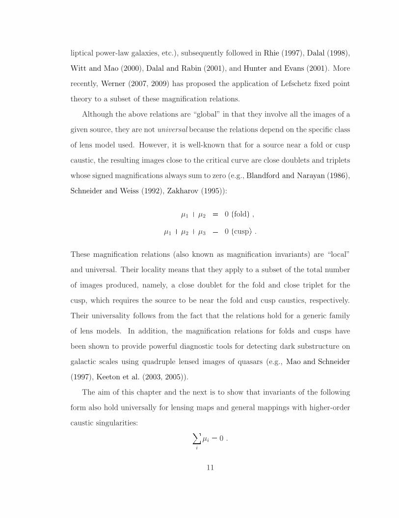
Schneider and Weiss (1992), Zakharov (1995)):

µ1 µ2 0 pfoldq ,µ1 µ2 µ3 0 pcuspq .

These magnification relations (also known as magnification invariants) are “local”

and universal. Their locality means that they apply to a subset of the total number

of images produced, namely, a close doublet for the fold and close triplet for the

cusp, which requires the source to be near the fold and cusp caustics, respectively.

Their universality follows from the fact that the relations hold for a generic family

of lens models. In addition, the magnification relations for folds and cusps have

been shown to provide powerful diagnostic tools for detecting dark substructure on

galactic scales using quadruple lensed images of quasars (e.g., Mao and Schneider

(1997), Keeton et al. (2003, 2005)).

The aim of this chapter and the next is to show that invariants of the following

form also hold universally for lensing maps and general mappings with higher-order

caustic singularities:

i

µi 0 .

11

In particular, it is shown that such invariants occur not only for folds and cusps,

but also for lensing maps with elliptic umbilic and hyperbolic umbilic caustics, and

for general mappings exhibiting any caustic appearing in Vladimir Arnold’s A,D,E

classification of caustic singularities. As an application, we use the hyperbolic umbilic

to show how such magnification relations can be used for substructure studies of

four-image lens galaxies. Before stating and proving the main theorem (Theorem 1

in Section 2.3), we begin by reviewing the necessary lensing and singular-theoretic

terminologies.

2.2 Basic Concepts

2.2.1 Lensing Theory

The spacetime geometry for gravitational lensing is treated as a perturbation of a

Friedmann universe by a “weak field” spacetime. To that end, we regard a grav-

itational lens as being localized in a very small portion of the sky. Furthermore,

we assume that gravity is “weak”, so that near the lens it can be described by a

Newtonian potential. We also suppose that the lens is static. Respecting these

assumptions, the spacetime metric is given by

gGL 1 2φ

c2

c2dτ 2 apτq2 1 2φ

c2

dR2

1 kR2R2

dθ2 sin2θ dϕ2

,

where τ is cosmic time, φ the time-independent Newtonian potential of the perturba-

tion caused by the lens, k is the curvature constant, and pR, θ, ϕq are the coordinates

in space. Here terms of order greater than 1c2 are ignored in any calculation involv-

ing φ.

The above metric is used to derive the time delay function Ty : L ÝÑ R, which

for a single lens plane is given by

Typxq 1

2|x y|2 ψpxq ,

12

where y ps1, s2q P S is the position of the source on the light source plane S R2,

x pu, vq P L is the impact position of a light ray on the lens plane L R2, and

ψ : L ÝÑ R is the gravitational lens potential. As its name suggests, the time

delay function gives the time delay of a lensed light ray emitted from a source in

S, relative to the arrival time of a light ray emitted from the same source in the

absence of lensing. Fermat’s principle yields that light rays emitted from a source

that reach an observer are realized as critical points of the time delay function. In

other words, a lensed image of a light source at y is a solution x P L of the equationpgradTyqpxq 0, where the gradient is taken with respect to x. When there is no

confusion with the mathematical image of a point, we shall follow common practice

and sometimes call a lensed image simply an image.

The time delay function also induces a lensing map η : L ÝÑ S, which is defined

by

x ÞÝÑ ηpxq x pgradψqpxq .We call ηpxq y the lens equation. Note that x P L is a solution of the lens equation

if and only if it is a lensed image because pgradTyqpxq ηpxq y. Critical points

of the lensing map η are those x P L for which detpJac ηqpxq 0. Generically, the

locus of critical points of the lensing map form curves called critical curves. The

value ηpxq of a critical point x under η is called a caustic point. These typically

form curves, but could be isolated points. Examples of caustics can be found in

Petters et al. (2001). For a generic lensing scenario, the number of lensed images

of a given source can change (by 2 for generic crossings) if and only if the source

crosses a caustic. The signed magnification of a lensed image x P L of a light source

at y ηpxq P S is given by

µpxq 1

detpJac ηqpxq (2.1)

13

Considering the graph of the time delay function, its principal curvatures coincide

with the eigenvalues of Hess Typxq. In addition, its Gaussian curvature at px, Typxqqequals detpHess Tyqpxq. In other words, the magnification of an image x can be

expressed as

µpxq 1

Gausspx, Typxqq , (2.2)

where y ηpxq, Gausspx, Typxqq is the Gaussian curvature of the graph of Ty at the

point px, Typxqq, and where we have used the fact that detpJac ηq detpHess Tyqfor single plane lensing. Therefore, the magnification relations are also geometric

invariants involving the Gaussian curvature of the graph of Ty at its critical points.

Readers are referred to Petters et al. (2001), Chapter 6, for a full treatment of these

aspects of lensing.

2.2.2 Higher-Order Caustic Singularities in Lensing

This section briefly reviews those aspects of the theory of singularities that will be

needed for our main theorem. It is also worth noting that the terms “universal” and

“generic” will be used often. Formally, a property is called generic or universal if it

holds for an open, dense subset of mappings in the given space of mappings. Elements

of the open, dense subset are then referred to as being generic (or universal). See

Petters et al. (2001), Chapter 8 for a discussion of genericity.

We saw in the previous section that the time delay function Typxq, which can be

viewed as a two-parameter family of functions with parameter y, gives rise to the

lensing map η : L ÝÑ S. The set of critical points of η consists of all x P L such that

detpJac ηqpxq 0. In this two-dimensional setting, a generic lensing map will have

only two types of generic critical points: folds and cusps (see Petters et al. (2001),

Chapter 8). The fold critical points map over to caustic arcs that abut isolated cusp

caustic points.

14

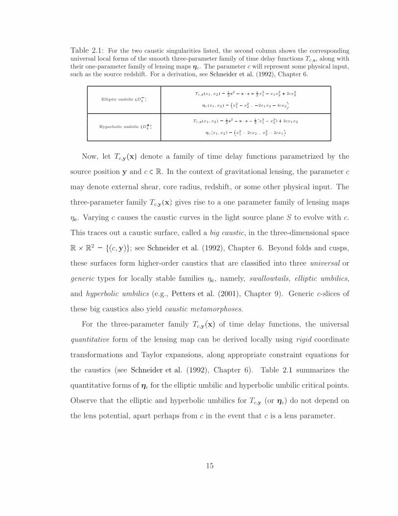
Table 2.1: For the two caustic singularities listed, the second column shows the correspondinguniversal local forms of the smooth three-parameter family of time delay functions Tc,s, along withtheir one-parameter family of lensing maps ηc. The parameter c will represent some physical input,such as the source redshift. For a derivation, see Schneider et al. (1992), Chapter 6.

Tc,spx1, x2q 12s2 x s 1

3x31 x1x2

2 2cx22

Elliptic umbilic pD4q

ηcpx1, x2q x21 x2

2 , 2x1x2 4cx2

Tc,spx1, x2q 1

2s2 x s 1

3px3

1 x32q 2cx1x2

Hyperbolic umbilic pD4q

ηcpx1, x2q x21 2cx2 , x2

2 2cx1

Now, let Tc,ypxq denote a family of time delay functions parametrized by the

source position y and c P R. In the context of gravitational lensing, the parameter c

may denote external shear, core radius, redshift, or some other physical input. The

three-parameter family Tc,ypxq gives rise to a one parameter family of lensing maps

ηc. Varying c causes the caustic curves in the light source plane S to evolve with c.

This traces out a caustic surface, called a big caustic, in the three-dimensional space

R R2 tpc,yqu; see Schneider et al. (1992), Chapter 6. Beyond folds and cusps,

these surfaces form higher-order caustics that are classified into three universal or

generic types for locally stable families ηc, namely, swallowtails, elliptic umbilics,

and hyperbolic umbilics (e.g., Petters et al. (2001), Chapter 9). Generic c-slices of

these big caustics also yield caustic metamorphoses.

For the three-parameter family Tc,ypxq of time delay functions, the universal

quantitative form of the lensing map can be derived locally using rigid coordinate

transformations and Taylor expansions, along appropriate constraint equations for

the caustics (see Schneider et al. (1992), Chapter 6). Table 2.1 summarizes the

quantitative forms of ηc for the elliptic umbilic and hyperbolic umbilic critical points.

Observe that the elliptic and hyperbolic umbilics for Tc,y (or ηc) do not depend on

the lens potential, apart perhaps from c in the event that c is a lens parameter.

15

2.2.3 Caustic Singularities of the A,D,E family

We can also consider general mappings. Consider a smooth k-parameter family

Fc,spxq of functions on an open subset of R2 that induces a smooth pk2q-parameter

family of mappings fcpxq between planes (k ¥ 2q. One uses Fc,s to construct a La-

grangian submanifold that is projected into the space tc, su Rk2R2. The caustics

of fc will then be the critical values of the projection (e.g., Golubitsky and Guillemin

(1973), Majthay (1985), Castrigiano and Hayes (2004), and Petters et al. (2001),

pp. 276–286). These projections are called Lagrangian maps, and they are differ-

entiably equivalent to fc. As mentioned in Chapter 1, Arnold classified all sta-

ble simple Lagrangian map-germs of n-dimensional Lagrangian submanifolds by

their generating family Fc,s (Arnold (1973), Arnold et al. (1985), pp. 330–331, and

Petters et al. (2001), p. 282). In the process he found a connection between his

classification and the Coxeter-Dynkin diagrams of the simple Lie algebras of types

An pn ¥ 2q, Dn pn ¥ 4q, E6, E7, E8. This classification is shown in Table 2.2. (The

classification of the elementary catastrophes, for codimension less than 5, was deter-

mined by Rene Thom in the 1960s.)

The fc shown in Table 2.2 are obtained from their corresponding Fc,s by taking

its gradient with respect to x and setting it equal to zero: gradpFc,sqpxq 0. This

equation is then rewritten in the form fcpxq s. We call x P R2 a pre-image of the

target point s P R2 if fcpxq s. Equivalently, this will be the case if and only if x is a

critical point of Fc,s (relative to a gradient in x). Next, we define the magnification

Mpx; sq at a critical point x of the family Fc,s by the reciprocal of the Gaussian

curvature at the point px, Fc,spxiqq in the graph of Fc,s:

Mpx; sq 1

Gausspx, Fc,spxqq Again, this makes it clear that magnification invariants are geometric invariants. In

16

Table 2.2: For each type of Coxeter-Dynkin diagram listed, indexed by n, the second columnshows the corresponding universal local forms of the smooth pn 1q-parameter family of generalfunctions Fc,s, along with their pn3q-parameter family of induced general maps fc between planes.This classification is due to Arnold (1973).

Fc,spx, yq xn1 y2 cn1xn1 c3x3 s2x2 s1x s2y

An pn ¥ 2qfcpx, yq pn 1qxn pn 1qcn1xn2 3c3x2 4yx , 2y

Fc,spx, yq x2y yn1 cn2yn2 c2y2 s2y s1x

Dn pn ¥ 4qfcpx, yq

2xy , x2 pn 1qyn2 pn 2qcn2yn3 2c2y

Fc,spx, yq x3 y4 c3xy2 c2y2 c1xy s2y s1x

E6

fcpx, yq 3x2 c3y2 c1y , 4y3 2c3xy 2c2y c1x

Fc,spx, yq x3 xy3 c4y4 c3y3 c2y2 c1xy s2y s1x

E7

fcpx, yq 3x2 y3 c1y , 3xy2 4c4y3 3c3y2 2c2y c1x

Fc,spx, yq x3 y5 c5xy3 c4xy2 c3y3 c2y2 c1xy s2y s1x

E8

fcpx, yq 3x2 c5y3 c4y2 c1y , 5y4 3c5xy2 2c4xy 3c3y2 2c2y c1x

addition, since the Gaussian curvature at the point pxi, Fc,spxiqq in the graph of Fc,s

is given by

Gausspxi, Fc,spxiqq detpHessFc,sqpxiq1 | gradFc,spxiq|2 ,

and since pxi, Fc,spxiqq is a critical point of the graph, we have that

Gausspxi, Fc,spxiqq det(HessFc,sqpxiq .Furthermore, a computation shows that for all the Fc,s shown in Table 2.2,

detpJac fcq detpHessFc,sq .Hence we can express the magnification in terms of fc:

Mpx; sq 1

detpJac fcqpxq (2.3)

17

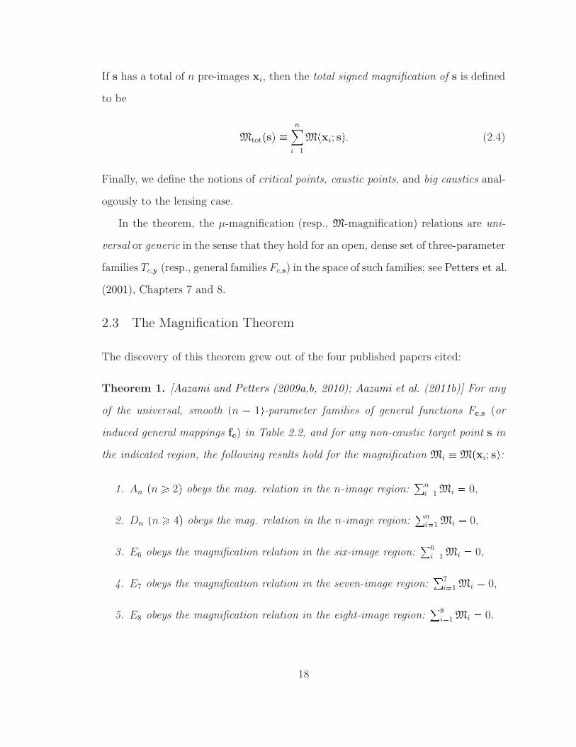
If s has a total of n pre-images xi, then the total signed magnification of s is defined

to be

Mtotpsq n

i1

Mpxi; sq. (2.4)

Finally, we define the notions of critical points, caustic points, and big caustics anal-

ogously to the lensing case.

In the theorem, the µ-magnification (resp., M-magnification) relations are uni-

versal or generic in the sense that they hold for an open, dense set of three-parameter

families Tc,y (resp., general families Fc,s) in the space of such families; see Petters et al.

(2001), Chapters 7 and 8.

2.3 The Magnification Theorem

The discovery of this theorem grew out of the four published papers cited:

Theorem 1. [Aazami and Petters (2009a,b, 2010); Aazami et al. (2011b)] For any

of the universal, smooth pn 1q-parameter families of general functions Fc,s (or

induced general mappings fc) in Table 2.2, and for any non-caustic target point s in

the indicated region, the following results hold for the magnification Mi Mpxi; sq:1. An pn ¥ 2q obeys the mag. relation in the n-image region:

°ni1 Mi 0,

2. Dn pn ¥ 4q obeys the mag. relation in the n-image region:°n

i1 Mi 0,

3. E6 obeys the magnification relation in the six-image region:°6

i1 Mi 0,

4. E7 obeys the magnification relation in the seven-image region:°7

i1 Mi 0,

5. E8 obeys the magnification relation in the eight-image region:°8

i1 Mi 0.

18

In addition, for the two smooth generic three-parameter families of time delay func-

tions Tc,y (or induced lensing maps ηc) in Table 2.3, and for any non-caustic tar-

get point s in the indicated region, the following results hold for the magnification

µi µpxi; sq:1. D

4 (Elliptic Umbilic) obeys the magnification relation in four-image region:

µ1 µ2 µ3 µ4 0.

2. D4 (Hyperbolic Umbilic) obeys the magnification relation in four-image region:

µ1 µ2 µ3 µ4 0.

Remarks. The results of Theorem 1 actually apply even when the non-caustic point

s is not in the maximum number of pre-images region. However, complex pre-images

will appear, which are unphysical in gravitational lensing. Note that for n ¥ 6 there

are Lagrangian maps that cannot be approximated by stable Lagrangian map-germs

Arnold (1973). As mentioned in Section 2.1, the fold pA2q and cusp pA3q magni-

fication relations are known (Blandford and Narayan (1986), Schneider and Weiss

(1992), Zakharov (1995)), but we restate them in the theorem for completeness.

2.4 Applications

Before discussing the applications, we recall that the magnification µi of a lensed

image is the flux Fi of the image divided by the flux FS of the unlensed source (e.g.,

Petters et al. (2001), pp. 82–85):

µi Fi

FS

,

where the “” choice is for even index images (minima and maxima) and the “”

choice is for odd index images (saddles). Though Fi is an observable, the source’s

flux FS is generally unknown. Consequently, the magnification µi is not directly

19

observable and so magnification sums°

i µi are also not observable. However, we

can construct an observable by introducing the following quantity:

R °i µi°

i |µi| °ipqFi°

i Fi

, (2.5)

where the choice is the same as above. This quantity is in terms of the observ-

able image fluxes Fi and image signs, which can be determined for real systems

Keeton et al. (2005, 2003).

Now, aside from their natural theoretical interest, the importance of magnifica-

tion relations in gravitational lensing arises in their applications to detecting dark

substructure in galaxies using “anomalous” flux ratios of multiply imaged quasars.

The setting consists typically of four images of a quasar lensed by a foreground

galaxy. The smooth mass density models used for the galaxy lens usually accurately

reproduce the number and relative positions of the images, but fail to reproduce

the image flux ratios. For the case of a cusp, where a close image triplet appears,

Mao and Schneider (1997) showed that the cusp µ-magnification relation fails (i.e.,

deviates from zero) and argued that it does so since the smoothness assumption

about the galaxy lens breaks down on the scale of the fold image doublet (this is

not the only interpretation; see also Evans and Witt (2003); Congdon and Keeton

(2005)). In other words, a violation of the cusp magnification relation in a real lens

system may imply a violation of smoothness in the lens, which in turn invokes the

presence of substructure or graininess in the galaxy lens on the scale of the image

separation. Soon thereafter Metcalf and Madau (2001) and Chiba (2002) showed

that dark matter was a plausible candidate for this substructure.

Keeton et al. (2003, 2005) then developed a rigorous theoretical framework show-

ing how the fold and cusp µ-magnification relations provide a diagnostic for detecting

substructure on galactic scales. Their analysis employs the R-quantity (2.5) for folds

20

and cusps:

Rfold µ1 µ2|µ1| |µ2| F1 F2

F1 F2, Rcusp µ1 µ2 µ3|µ1| |µ2| |µ3| F1 F2 F3

F1 F2 F3,

where Fi is the observable flux of image i and image 2 has negative parity. For

a source sufficiently close to a fold (resp., cusp) caustic, the images will have a

close image pair (resp., close image triplet); see the close doublets and triplets in

Figure 2.1(a,b,d,e). Theoretically, these images should have vanishing Rfold and

Rcusp due to the fold and cusp magnification relations and so nontrivial deviations

from zero would signal the presence of substructure. In Keeton et al. (2003, 2005),

it was shown that 5 of the 12 fold-image systems and 3 of the 4 cusp-image ones

showed evidence for substructure.

The study above would look at a multiple-image system and consider subsets of

two and three images to analyze Rfold and Rcusp, respectively. Such analyses are

then “local” when more than three images occur since only two or three images are

studied at a time. Theorem 1 generalizes the above R-quantities from folds and

cusps to generic smooth lens systems that exhibit swallowtail, elliptic umbilic, and

hyperbolic umbilic singularities. The R-quantities resulting from these higher-order

singularities allow one to consider four images at a time and so are more global

than the fold and cusp relations in terms of how many images are incorporated.

The singularity that is most applicable to observed quadruple-images produced by

the lensing of quasars is the hyperbolic umbilic (cf. Figure 2.1). The associated

R-quantity is

Rh.u. µ1 µ2 µ3 µ4|µ1| |µ2| |µ3| |µ4| F1 F2 F3 F4

F1 F2 F3 F4,

where images 2 and 4 have negative parity.

We now illustrate the hyperbolic umbilic quantity Rh.u. using a well-known model

for a galaxy lens, namely, a singular isothermal ellipsoid (SIE) lens. The SIE lens

21

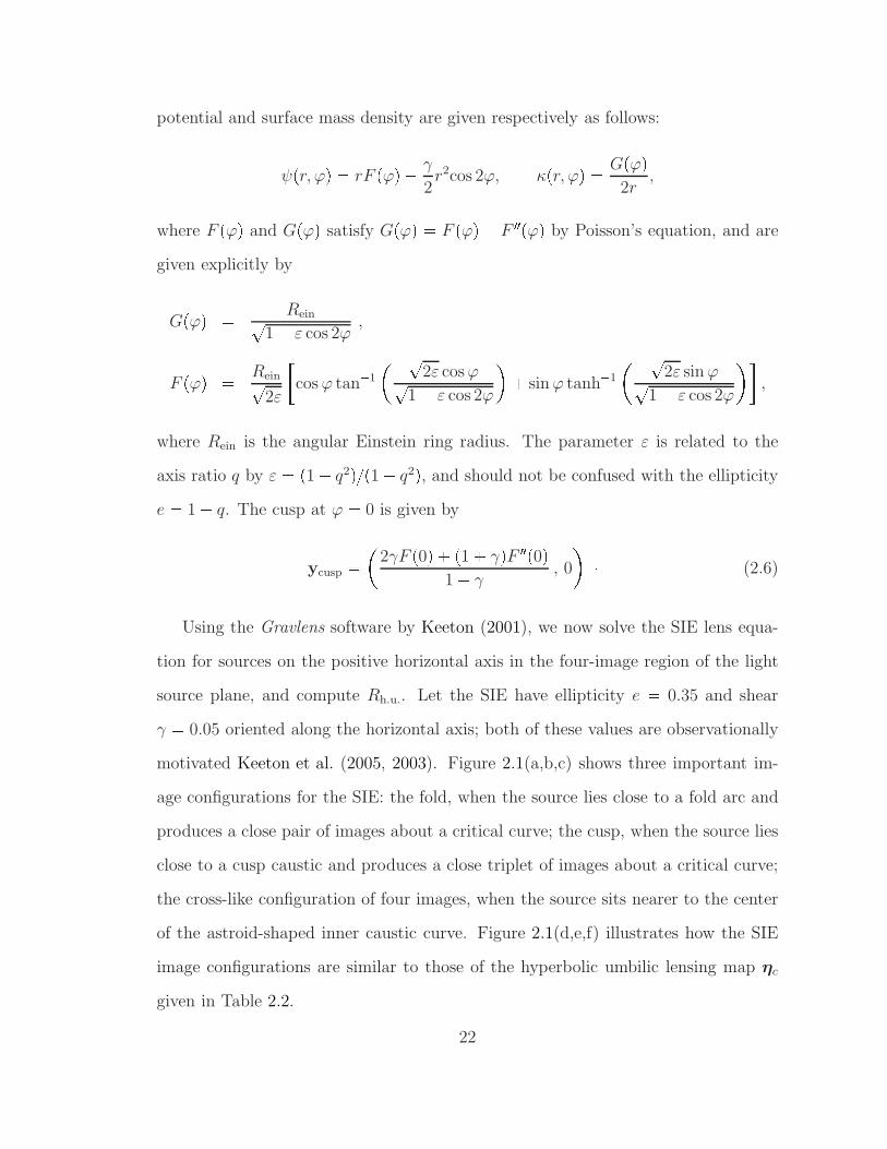
potential and surface mass density are given respectively as follows:

ψpr, ϕq rF pϕq γ

2r2cos 2ϕ, κpr, ϕq Gpϕq

2r,

where F pϕq and Gpϕq satisfy Gpϕq F pϕq F 2pϕq by Poisson’s equation, and are

given explicitly by

Gpϕq Rein?1 ε cos 2ϕ

,

F pϕq Rein?2ε

cosϕ tan1

?2ε cosϕ?

1 ε cos 2ϕ

sinϕ tanh1

?2ε sinϕ?

1 ε cos 2ϕ

,

where Rein is the angular Einstein ring radius. The parameter ε is related to the

axis ratio q by ε p1 q2qp1 q2q, and should not be confused with the ellipticity

e 1 q. The cusp at ϕ 0 is given by

ycusp 2γF p0q p1 γqF 2p0q

1 γ, 0

(2.6)

Using the Gravlens software by Keeton (2001), we now solve the SIE lens equa-

tion for sources on the positive horizontal axis in the four-image region of the light

source plane, and compute Rh.u.. Let the SIE have ellipticity e 0.35 and shear

γ 0.05 oriented along the horizontal axis; both of these values are observationally

motivated Keeton et al. (2005, 2003). Figure 2.1(a,b,c) shows three important im-

age configurations for the SIE: the fold, when the source lies close to a fold arc and

produces a close pair of images about a critical curve; the cusp, when the source lies

close to a cusp caustic and produces a close triplet of images about a critical curve;

the cross-like configuration of four images, when the source sits nearer to the center

of the astroid-shaped inner caustic curve. Figure 2.1(d,e,f) illustrates how the SIE

image configurations are similar to those of the hyperbolic umbilic lensing map ηc

given in Table 2.2.

22

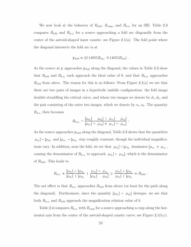
We now look at the behavior of Rfold, Rcusp, and Rh.u. for an SIE. Table 2.3

compares Rfold and Rh.u. for a source approaching a fold arc diagonally from the

center of the astroid-shaped inner caustic; see Figure 2.1(a). The fold point where

the diagonal intersects the fold arc is at

yfold p0.14055Rein, 0.14055Reinq .As the source at y approaches yfold along the diagonal, the values in Table 2.3 show

that Rfold and Rh.u. each approach the ideal value of 0, and that Rh.u. approaches

Rfold from above. The reason for this is as follows: From Figure 2.1(a) we see that

there are two pairs of images in a hyperbolic umbilic configuration: the fold image

doublet straddling the critical curve, and whose two images we denote by d1, d2, and

the pair consisting of the outer two images, which we denote by o1, o2. The quantity

Rh.u. then becomes

Rh.u. |µd1| |µd2| |µo1| |µo2||µd1| |µd2| |µo1| |µo2| As the source approaches yfold along the diagonal, Table 2.3 shows that the quantities|µd1| |µd2| and |µo1| |µo2| stay roughly constant, though the individual magnifica-

tions vary. In addition, near the fold, we see that |µd1| |µd2| dominates |µo1| |µo2|,causing the denominator of Rh.u. to approach |µd1| |µd2|, which is the denominator

of Rfold. This leads to

Rh.u. |µd1| |µd2||µd1| |µd2| |µo3| |µo4||µd1| |µd2| ¥ |µd1| |µd2||µd1| |µd2| Rfold .

The net effect is that Rh.u. approaches Rfold from above (at least for the path along

the diagonal). Furthermore, since the quantity |µd1| |µd2| diverges, we see that

both Rh.u. and Rfold approach the magnification relation value of 0.

Table 2.4 compares Rh.u. with Rcusp for a source approaching a cusp along the hor-

izontal axis from the center of the astroid-shaped caustic curve; see Figure 2.1(b,c).

23

Table 2.3: The quantities Rh.u. and Rfold for an SIE with e 0.35 and γ 0.05 oriented along thehorizontal axis. The source approaches the fold point yfold p0.14055Rein, 0.14055Reinq diagonallyfrom the center of the astroid-shaped inner caustic. The quantity |µd1

| |µd2| is the difference in

the magnifications of the images in the close doublet, while |µo1| |µo2

| is the difference for theremaining two outer images; cf. Figure 2.1(a).

Source Rfold Rh.u. |µd1| |µd2

| |µo1| |µo2

| |µd1| |µd2

| |µo1| |µo2

|(0.10Rein , 0.10Rein) 0.14 0.19 1.22 1.21 8.51 4.35(0.11Rein , 0.11Rein) 0.13 0.18 1.22 1.22 9.64 4.28(0.12Rein , 0.12Rein) 0.11 0.15 1.22 1.22 11.55 4.21(0.13Rein , 0.13Rein) 0.08 0.12 1.22 1.22 15.83 4.15(0.14Rein , 0.14Rein) 0.02 0.04 1.21 1.23 65.17 4.081

(0.1405Rein , 0.1405Rein) 0.008 0.015 1.21 1.23 156.80 4.078

For these values of the ellipticity and shear, we see from (2.6) that the two cusps on

the horizontal axis are located at

ycusp p0.48Rein, 0q . (2.7)

The table shows that as the source approaches ycusp along the horizontal axis, the

quantity Rh.u. approaches Rfold from below. In other words, Rh.u. is smaller than Rfold.

To see why this happens, consider the triplet of sub-images in Figure 2.1(b), which

we denote by t1, t2, t3, and the extra outer image, denote by o. With this notation,

Rh.u. |µt1| |µt2| |µt3| |µo||µt1| |µt2| |µt3| |µo| As the source approaches ycusp along the horizontal axis, the values in Table 2.4 of

the cusp relation |µt1| |µt2| |µt3| are positive. The inclusion of the outer, negative

parity magnification µo then subtracts from that positive value, yieldingp|µt1| |µt2| |µt3|q |µo| ¤ |µt1| |µt2| |µt3| ,which implies that

Rh.u. ¤ Rcusp .

Furthermore, Table 2.4 shows that |µo| grows fainter faster than the value of the

signed magnification of the triplet, which yields|µt1| |µt2| |µt3| " |µo| .24

Table 2.4: The quantities Rh.u. and Rcusp for an SIE with e 0.35 and γ 0.05 oriented alongthe horizontal axis. The source approaches the cusp point ycusp p0.48Rein, 0q along the horizontalaxis from the center of the astroid-shaped inner caustic. The quantity |µt1| |µt2 | |µt3 | is thesigned magnification sum of the cusp triplet, while |µo| is the magnification of the outer image; seeFigure 2.1(b).

Source Rcusp Rh.u. |µt1| |µt2

| |µt3| |µt1

| |µt2| |µt3

| |µo1|

(0 , 0) pcenterq 0.52 0.23 8.49 4.46 2.02(0.10Rein , 0) 0.41 0.22 9.58 3.94 1.49(0.15Rein , 0) 0.36 0.21 10.57 3.76 1.29(0.20Rein , 0) 0.30 0.19 12.02 3.61 1.12(0.25Rein , 0) 0.25 0.17 14.20 3.48 0.98(0.30Rein , 0) 0.19 0.14 17.71 3.38 0.85(0.35Rein , 0) 0.14 0.10 24.10 3.30 0.74(0.40Rein , 0) 0.08 0.07 39.02 3.23 0.64(0.45Rein , 0) 0.03 0.02 111.5 3.18 0.55

In other words, as the source approaches ycusp along the horizontal axis, the contri-

bution of the outer image |µo| to the numerator and denominator of Rh.u. becomes

negligible. The net effect, at least for the given horizontal axis approach, is that Rh.u.

and Rcusp converge, with Rh.u. approaching Rcusp from below as they both approach

the magnification relation value of 0.

Finally, though Rh.u. can approximate Rfold and Rcusp for fold image doublets and

cusp image triplets, resp., the hyperbolic umbilic magnification relation has a more

global reach in terms of the number of images included. This is because Rh.u. also

applies directly to image configurations that are neither close doublets nor triplets;

e.g., to cross-like configurations as in Figure 2.1(c). For instance, it was determined

in Keeton et al. (2003) that to satisfy the relation |Rcusp| 0.1 at 99% confidence,

the opening angle must be θ 30. By opening angle we mean the angle of the

polygon spanned by the three images in the cusp triplet, measured from the position

of the lens galaxy, which in our case, is centered at the origin in the lens plane.

For the SIE cross-like configuration shown in Figure 2.1(c), the opening angle is

θ 140; a perfect cross, which would be the case if the source were centered inside

the astroid-shaped inner caustic, has θ 180. In other words, to satisfy the cusp

relation reasonably well, the cusp triplet must be quite tight as, for example, in

the SIE cusp triplet shown in Figure 2.1(b). By contrast, the quantity Rh.u. applies

even for values θ " 30. (In Table 2.4 note how Rh.u. is smaller than Rcusp for source

25

positions closer to the center p0, 0q, which yield more cross-like image configurations.)

A more detailed study of the properties of Rh.u. would involve a Monte Carlo

analysis similar to that employed in Keeton et al. (2005, 2003) to study Rcusp and

Rfold.

26

SIE for e 0.35 , γ 0.05 Hyperbolic Umbilic ηc for c 0.2

(a) fold (d) fold

+

+

-

(b) cusp (e) cusp

+

+

-

(c) cross (f) cross

+

+

-

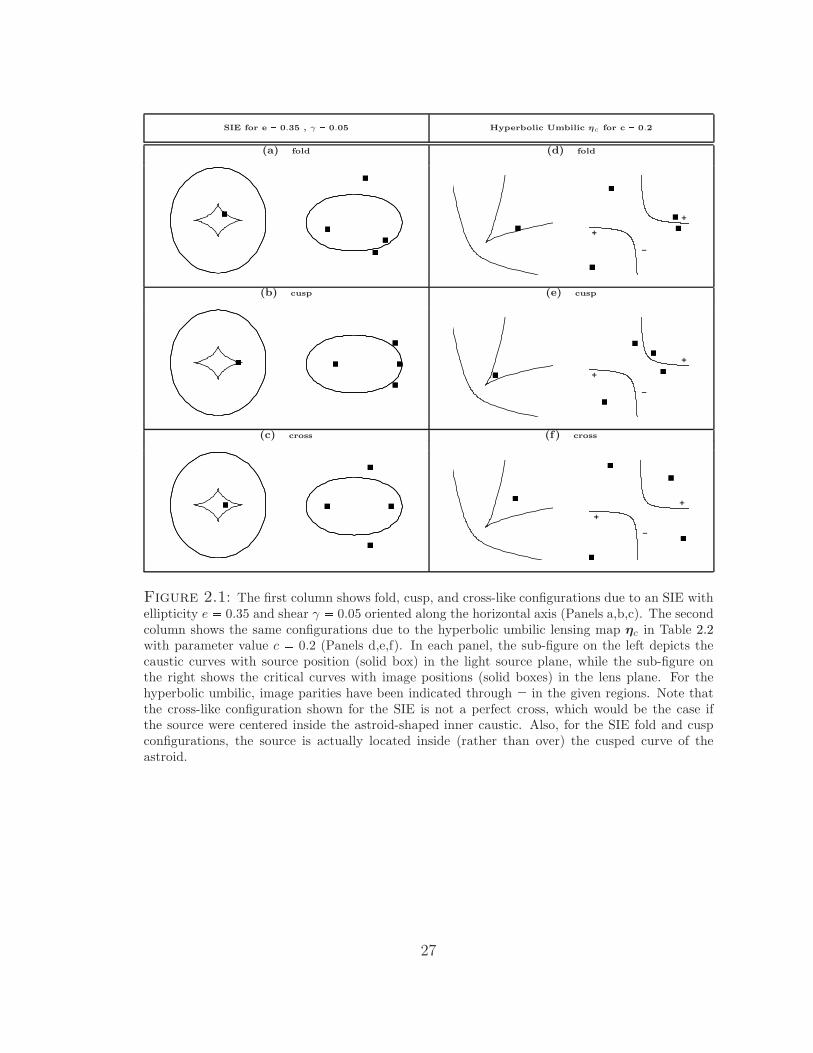
Figure 2.1: The first column shows fold, cusp, and cross-like configurations due to an SIE withellipticity e 0.35 and shear γ 0.05 oriented along the horizontal axis (Panels a,b,c). The secondcolumn shows the same configurations due to the hyperbolic umbilic lensing map ηc in Table 2.2with parameter value c 0.2 (Panels d,e,f). In each panel, the sub-figure on the left depicts thecaustic curves with source position (solid box) in the light source plane, while the sub-figure onthe right shows the critical curves with image positions (solid boxes) in the lens plane. For thehyperbolic umbilic, image parities have been indicated through in the given regions. Note thatthe cross-like configuration shown for the SIE is not a perfect cross, which would be the case ifthe source were centered inside the astroid-shaped inner caustic. Also, for the SIE fold and cuspconfigurations, the source is actually located inside (rather than over) the cusped curve of theastroid.

27

3

Proof of Magnification Theorem

3.1 An Algebraic Proposition

3.1.1 A Recursive Relation for Coefficients of Coset Polynomials

We will make repeated use of the Euler trace formula to prove Theorem 1, by first

establishing a proposition about polynomials that will yield the Euler trace formula

as a corollary.

We begin with some notation. Let Crxs be the ring of polynomials over C and

consider a polynomial

ϕpxq anxn a1x a0 P Crxs .

Suppose that the n zeros x1, . . . , xn pf ϕpxq are distinct (generically, the roots of a

polynomial are distinct) and let ϕ1pxq be the derivative of ϕpxq. Also, let R Cpxqdenote the subring of rational functions that are defined at the roots xi of ϕpxq:

R "ppxqqpxq : ppxq, qpxq P Crxs and qpxiq 0 for all roots xi

* Let pϕpxqq be the ideal in R generated by ϕpxq and denote the cosets of the quo-

tient ring Rpϕpxqq using an overbar. Below are two basic results that we prove in

28

Section 3.1.2 below for the convenience of the reader:

• Members of the same coset in Rpϕpxqq agree on the roots xi of ϕpxq, that is,

if h1pxq and h2pxq belong to the same coset, then h1pxiq h2pxiq.• Every rational function hpxq P R has in its coset hpxq P Rpϕpxqq a unique

polynomial representative hpxq of degree less than n.

Proposition 2. Consider any polynomial ϕpxq anxn a1x a0 P Crxs with

distinct roots and any rational function hpxq P R. Let

hpxq cn1xn1 c1x c0

be the unique polynomial representative of the coset hpxq P Rpϕpxqq and let

rpxq bn1xn1 b1x b0

be the unique polynomial representative of the coset ϕ1pxqhpxq P Rpϕpxqq. Then the

coefficients of rpxq are given in terms of the coefficients of hpxq and ϕpxq through

the following recursive relation:

bni cn1bni,n1 c1bni,1 c0bni,0 i 1, . . . , n , (3.1)

with$'&'% bni,0 pn pi 1qq anpi1q , i 1, . . . , n ,

bni,k ani

an

bn1,k1 bnpi1q,k1 , i 1, . . . , n , k 1, . . . , n 1 ,(3.2)

where b1,k1 0.

By Proposition 2, if rkpxq is the unique polynomial representative of the coset

ϕ1pxqxk P Rpϕpxqq, then

rkpxq bn1,kxn1 b1,kx b0,k , k 0, 1, . . . , n 1 , (3.3)

where its coefficients are given in terms of the coefficients of ϕpxq through (3.2).

29

Corollary 3. Assume the hypotheses and notation of Proposition 2. Given the

distinct roots x1, . . . , xn of ϕpxq, the Newton sums Nk °ni1pxiqk satisfy:

Nk bn1,k

an

, k 0, 1, . . . , n 1 . (3.4)

In other words, the quantity anNk equals the pn 1qst coefficient of the unique

polynomial representative (3.3) of the coset ϕ1pxqxk in Rpϕpxqq.Proof. Note that for k 0, eqn. (3.2) in Proposition 2 yields

bn1,0 nan N0an .

For 1 ¤ k ¤ n1, there is a known recursive relation forNk, in terms ofN1, . . . , Nk1;

see, e.g., Barbeau (2003), p. 203. It is given by

kank ank1N1 ank2N2 an1Nk1 anNk 0 . (3.5)

We proceed by induction on k for 1 ¤ k ¤ n 1. For k 1, eqn. (3.5) implies

N1 an1

an, while eqn. (3.2) gives bn1,1 an1 anN1, which agrees with eqn.

(3.4). Now assume that bn1,j anNj for j 1, . . . , k 1. To establish the result

30

for j k, we shall repeatedly apply Proposition 2:

bn1,k an1

an

bn1,k1 bn2,k1 an1

an

bn1,k1 an2

an

bn1,k2 bn3,k2

an1

an

bn1,k1 an2

an

bn1,k2 an3

an

bn1,k3 bn4,k3

... an1

an

bn1,k1 an2

an

bn1,k2 an3

an

bn1,k3 anpk1qan

bn1,1 ank

an

bn1,0 bnpk1q,0 . an1Nk1 an2Nk2 an3Nk3 anpk1qN1 kank

anNk ,

where bn1,0 nan and bnpk1q,0 pn kqank follow from eqn. (3.2) in Proposi-

tion 2, and the last equality is due to (3.5).

Corollary 4 (Euler Trace Formula). Assume the hypotheses and notation of Propo-

sition 2. For any rational function hpxq P R, the following holds:

n

i1

hpxiq bn1

an

, (3.6)

where bn1 is the pn 1qst coefficient of the unique polynomial representative rpxq of

the coset ϕ1pxq hpxq P Rpϕpxqq and an the nth coefficient of ϕpxq.Proof. Let hpxq be the unique polynomial representative of the coset hpxq PRpϕpxqq. First note that, since hpxq and hpxq belong to the same coset, we have

hpxiq hpxiq. The Euler trace formula now proceeds from a simple application of

31

Propositon 2 and Corollary 3:

n

i1

hpxiq n

i1

hpxiq n

i1

n1

j0

cj pxiqj n1

j0

cj

n

i1

pxiqj n1

j0

cjNj cn1Nn1 c1N1 c0N0 cn1

bn1,n1

an

c1

bn1,1

an

c0

bn1,0

an

(by Cor. 3) cn1bn1,n1 c1bn1,1 c0bn1,0

an bn1

an

(by Proposition 2)

Remark. Dalal and Rabin (2001) gave a different proof of the Euler trace formula,

one employing residues.

3.1.2 Proof of Proposition 2

We begin with some preliminaries about quotient rings to make the proof more

self-contained. Let Crxs be the ring of polynomials over C and let Cpxq be the

field of rational functions formed from quotients of polynomials in Crxs. The n

zeros x1, . . . , xn of ϕpxq anxn a1x a0 P Crxs are assumed to be distinct

(generically, the roots of a polynomial are distinct). Let pϕpxqq denote the ideal in

Crxs generated by ϕpxq, and consider the quotient ring Crxspϕpxqq, whose cosets

we denote by gpxq. This quotient ring has two important properties:

• Property 1: If g1pxq g2pxq, then by definition g1pxq g2pxq hpxqϕpxq for

some hpxq P Crxs, from which it follows that g1pxiq g2pxiq for all n roots xi

of ϕpxq. Thus members of the same coset must agree on the roots of ϕpxq, so

that, in particular,°n

i1 g1pxiq °n

i1 g2pxiq.32

• Property 2: Each coset gpxq has a unique representative of degree at most n1,

as follows: by the division algorithm in Crxs, there exist polynomials qpxq and

rpxq such that

gpxq qpxqϕpxq rpxq ,where deg r deg ϕ n. Passing to the quotient ring Crxspϕpxqq, we see

that gpxq rpxq. Suppose now that there exists another polynomial ppxq of

degree less than n with gpxq ppxq. Then ppxq rpxq, so that

ppxq rpxq hpxqϕpxqfor some hpxq P Crxs. If hpxq 0, then deg hϕ ¥ n, while the degree of the

left-hand side is less than n. We must therefore have hpxq 0 and ppxq rpxq.We may thus represent every coset by its unique polynomial representative of

degree less than n, which in turn implies that Crxspϕpxqq is a vector space of

dimension n, with basis!1, x, x2 . . . , xn1

).

The next result will be used to show that Properties 1 and 2 also hold for a

certain subset of rational functions in Cpxq (see Claim 2 below).

Claim 1. Let x1, . . . , xn P C be distinct. Let c1, . . . , cn P C, not necessarily distinct.

Then there exists a unique polynomial Hpxq P Crxs with deg h n such that

Hpxiq ci.

Proof (Claim 1). Induction on n. For n 1, define Hpxq c1. Now assume that the

result is true for n 1, and consider a set of n distinct complex numbers x1, . . . , xn.

By the induction hypothesis, there exists a polynomial hpxq P Crxs with deg h n1

such that hpxiq ci for i 1, . . . , n 1. Now define

Hpxq hpxq px x1qpx x2q px xn1qpxn x1qpxn x2q pxn xn1q pcn hpxnqq .33

It follows that Hpxq P Crxs has degree less than n, and Hpxiq ci for all i 1, . . . , n.

(As a simple example to show that Hpxq need not be unique if the x1, . . . , xn are not

distinct, consider the numbers 2, 2, 3, 3 all being mapped to 0. Then the polynomials

H1pxq px 2q2px 3q, H2pxq px 2qpx 3q2, and H3pxq px 2qpx 3q all

satisfy the assumptions of the lemma.) Suppose that there exist two polynomials

H1pxq and H2pxq with H1pxiq ci H2pxiq. By the division algorithm in Crxs,there are unique polynomials qpxq and rpxq such that

H1pxq H2pxq qpxq rpx x1qpx x2q px xnqs rpxq ,where deg r n. If qpxq 0, then the degree of the polynomial on the right-hand

side is at least n, whereas H1pxq H2pxq has degree less than n. We must therefore

have qpxq 0. Moreover, if rpxq 0, then H1pxiq H2pxiq gives that rpxiq 0

for all x1, . . . , xn. This implies, however, that rpxq has n distinct zeros and so must

have degree n, a contradiction. Thus H1pxq H2pxq. (Claim 1)

Let R Cpxq denote the subring of rational functions that are defined at the

roots xi of ϕpxq,R "

ppxqqpxq : ppxq, qpxq P Crxs and qpxiq 0 for all roots xi

*,

and consider the quotient ring Rpϕpxqq. The next claim states that the ring

Rpϕpxqq satisfies Properties 1 and 2.

Claim 2. Members of the same coset in Rpϕpxqq agree on the roots xi of ϕpxq,that is, if g1pxq and g2pxq belong to the same coset, then g1pxiq g2pxiq, and so°n

i1 g1pxiq °ni1 g2pxiq. In addition, any rational function hpxq P R will have in

its coset hpxq P Rpϕpxqq a unique polynomial representative rpxq of degree less than

n.

34

Proof (Claim 2). Notice that, if h1pxq h2pxq P Rpϕpxqq, then by definition there

exists a rational function hpxq P R such that

h1pxq h2pxq hpxqϕpxq ,so that h1pxiq h2pxiq for all the zeros xi of ϕpxq. In other words, Rpϕpxqq also

satisfies Property 1. It turns out that when the zeros x1, . . . , xn of ϕpxq are distinct,

as we are assuming they are, then Rpϕpxqq also satisfies Property 2 (in fact Rpϕpxqqand Crxspϕpxqq will be isomorphic as rings). For given a coset hpxq P Rpϕpxqq,Claim 1 shows that there is a unique polynomial gpxq P Crxs of degree less than n

whose values at the n roots xi are hpxiq. Then the rational function gpxq hpxq P Rvanishes at every xi, and a simple application of the division algorithm applied

to the numerator of gpxq hpxq shows that gpxq hpxq P Rpϕpxqq. Thus any

rational function hpxq P R will have in its coset hpxq P Rpϕpxqq a unique polynomial

representative rpxq of degree less than n. (Claim 2)

We now begin the proof of the Proposition by establishing the following Lemma:

Lemma. Let ϕpxq anxn a1x a0 and consider the quotient ring Rpϕpxqq.

For any 1 ¤ k ¤ n 1, let

rkpxq bn1,k xn1 b1,k x b0,k

be the unique polynomial representative in the coset ϕ1pxqxk. Then the following

recursive relation holds:$'&'% bni,0 pn pi 1qq anpi1q , i 1, . . . , n ,

bni,k ani

an

bn1,k1 bnpi1q,k1 , i 1, . . . , n , k 1, . . . , n 1 ,(3.7)

where b1,k1 0.

35

Proof of Lemma. The existence and uniqueness of the polynomial

rkpxq bn1,k xn1 bni,k x

ni b1,k x b0,k 1 ,

where

ϕ1pxq xk rkpxq bn1,k xn1 bni,k xni b1,kx b0,k 1 , (3.8)

were established in Claim 2. Also, note that since ϕpxq 0 P Rpϕpxqq, we have

xn an1

an

xn1 a1

an

x a0

an

1 . (3.9)

Case k 0: By (3.8), we get

ϕ1pxqx0 r0pxq bn1,0 xn1 bni,0 xni b1,0 x b0,0 1 .

However,

ϕ1pxqx0 ϕ1pxq nan xn1 pn pi 1qqanpi1q xni 2a2 x a1 1 .

Consequently,

bni,0 pn pi 1qq anpi1q , i 1, . . . , n . (3.10)

Case k 1, . . . , n 1: Equations (3.8) and (3.9) yield

ϕ1pxq xk bn1,k xn1 bni,k xni b1,k x b0,k 1 xϕ1pxq xk1 xbn1,k1 xn1 bn2,k1 xn2 b1,k1 x b0,k1 1

bn1,k1 xn bn2,k1 xn1 b1,k1 x2 b0,k1 x bn1,k1

an1

an

xn1 a1

an

x a0

an

1

bn2,k1 xn1 b1,k1 x2 b0,k1 x n

i1

ani

an

bn1,k1 bnpi1q,k1

xni .

36

The coefficients of (3.8) are then related to the coefficients of ai of ϕpxq as follows:

bni,k ani

an

bn1,k1 bnpi1q,k1 , i 1, . . . , n , k 1, . . . , n 1 ,

where the coeffiencients bni,0 are given by (3.10). Note that bn,k 0 since the unique

polynomial goes up to degree n 1. (Lemma)

We now complete the proof of the Proposition. If h1,pxq and h2,pxq are the

unique polynomial representatives of the cosets h1pxq and h2pxq, respectively, then

by uniqueness, the sum h1,pxq h2,pxq is the unique polynomial representative of

the coset h1pxq h2pxq. With that said, we note that, since hpxq hpxq, it follows

that rpxq ϕ1pxqhpxq ϕ1pxqhpxq. We thus have

rpxq ϕ1pxqhpxq cn1ϕ1pxqxn1 c1ϕ1pxqx c0ϕ1pxq cn1rn1pxq c1r1pxq c0r0pxq cn1

n

i1

bni,n1xni c1

n

i1

bni,1xni c0

n

i1

bni,0xni n

i1

pcn1bni,n1 c1bni,1 c0bni,0q xni n

i1

bnixni . (Proposition)

3.2 Algebraic Proof of Magnification Theorem

We are now ready to prove our Main Theorem. We begin by establishing some

preliminaries before starting the computational part of the proof.

Recall from Section 2.2.3 that given a family of functions Fc,s, a parameter vectorpc0, s0q is called a caustic point of the family if there is at least one critical point x0

of Fc0,s0 (i.e., x0 satifies gradpFc0,s0qpx0q 0) such that the Gaussian curvature at

37

px0, Fc,spx0qq in the graph of Fc,s vanishes. Equivalently, pc0, s0q will be a caustic

point if detpJac fcqpx0q vanishes, since

Gausspx0, Fc,spx0qq detpJac fcqpx0q .Now, given an induced mapping fc and a target point s ps1, s2q, we can use the

pair of equations ps1, s2q fcpx, yq pf p1qc px, yq, f p2qc px, yqqto solve for px, yq in terms of ps1, s2q, which will give the pre-images xi pxi, yiqof s under fc. For the singularities in Table 2.2, we shall see that the pre-images

can be determined from solutions of a polynomial in one variable, which is obtained

by eliminating one of the pre-image coordinates, say y. In doing so we obtain a

polynomial ϕpxq P Crxs whose roots will be the x-coordinates xi of the different

pre-images under fc:

ϕpxq anxn a1x a0 .

Generically, we can assume that the roots of ϕpxq are distinct, an assumption made

throughout the paper.

We would then be able to express the magnification Mpx, y; sq at a general pre-

image point px, yq as a function of one variable, in this case x, so that

Mpx, ypxq; sq 1

Jpx, ypxqq 1

Jpxq Mpxq ,where J detpJac fcq and the explicit notational dependence on s is dropped for

simplicity (recall eqn. (2.3) in Section 2.2.3). Since we shall consider only non-

caustic target points s giving rise to pre-images pxi, ypxiqq, we know that Jpxiq 0.

Furthermore, we shall only consider non-caustic points that yield the maximum

number of pre-images. In addition, for the singularities in Table 2.2, the rational

function Mpxq is defined at the roots of ϕpxq, i.e., Mpxq P R. Now, denote by mpxq38

the unique polynomial representative in the coset ϕ1pxqMpxq P Rpϕpxqq, and let

bn1 be its pn1qst coefficient. In the notation of Proposition 2, we have hpxq Mpxqand rpxq mpxq. Euler’s trace formula (Corollary 3.6) then tells us immediately

that the total signed magnification satisfies

i

Mi bn1

an

(3.11)

It therefore remains to determine the coefficient bn1 for each caustic singularity in

Table 2.2. Next to each singularity below we indicate the value of n 1, which is

the codimension of the singularity.

Finally, we mention that the full theorem is not a direct consequence of the Euler-

Jacobi formula, of multi-dimensional residue integral methods, or of Lefschetz fixed

point theory, because some of the singularities have fixed points at infinity. We will

address these issues in greater detail in our geometric proof of Main Theorem in

Section 3.3 below. We now begin the proof of Theorem 1.

Consider first the singularities of type An. Since the cases n 2, 3 are known,

we will consider n ¥ 4 here. The pn 1q-parameter family of general functions FAn

is given in Arnold (1973) by

FAnpx, yq xn1 y2 cn1xn1 cn2x

n2 c3x3 c2x

2 c1x. (3.12)

To convert this into the form shown in Table 2.2, we use the following coordinate

transformation on the domain tpx, yqu R2:px, yq ÞÝÑ

x, y c2

2

. (3.13)

This transforms eqn. (3.12) to

FAn

c,s px, yq xn1 y2 cn1xn1 c3x

3 s2x2 s1x s2y , (3.14)

39

where c1 s1 and c2 s2. The parameters s1, s2 are to be interpreted in the

context of gravitational lensing as the rectangular coordinates on the source plane

S R2. Note that we omitted the constant term from eqn. (3.14) since it will not

affect any of our results below. Note also that

detHessFAn

detHessFAn

c,s

,

so that the magnification (as defined in eqn. (2.3)) is unaltered. We will work with

the form of FAnc,s in eqn. (3.14). The corresponding pn3q-parameter family of general

mappings fAnc : R2 ÝÑ R2 is

fAn

c px, yq pn 1qxn pn 1qcn1xn2 3c3x

2 4yx , 2y ps1, s2q.

Here s ps1, s2q is a non-caustic target point lying in the region with the maximum

number of lensed images. Since s2 2y, we can eliminate y to obtain a polynomial

in the variable x:

ϕAnpxq pn 1qxn pn 1qcn1x

n2 3c3x2 2s2x s1 , (3.15)

whose n roots are the x-coordinates of the lensed images xi of s. The Jacobian

determinant of fAnc expressed in the single variable x is

detJac fAn

c

2npn 1qxn1 pn 2qpn 1qcn1x

n3 6c3x 2s2

.

(3.16)

A comparison of eqns. (3.15) and (3.16) then shows that2ϕ1Anpxq det

Jac fAn

c

pxq 1

Mpxq We thus have

ϕ1AnpxqMpxq 1

2

40

Thus the unique polynomial representative of the coset ϕ1AnpxqMpxq is the polynomial

mpxq 12, whose pn 1qst coefficient is bn1 0 for all n ¥ 4. Euler’s trace

formula in the form of eqn. (3.11) then tells us that the total signed magnification is

n

i1

Mi 0 , pAn, n ¥ 2q.For typeDn, n ¥ 4, the corresponding pn3q-parameter family of induced general

maps fDn

c : R2 ÝÑ R2 is shown in Table 2.2:

fDn

c px, yq 2xy , x2 pn 1qyn2 pn iqcniy

npi1q 2c2y ps1, s2q. (3.17)

Once again the point s ps1, s2q is a non-caustic target point lying in the region

with the maximum number of lensed images. This time, however, we eliminate x to

obtain a polynomial in the variable y:

ϕDnpyq 4pn 1qyn 4pn 2qcn2y

n1 4pn iqcniynpi1q 8c2y

3 4s2y2 s2

1 ,

whose n roots are the y-coordinates of the n lensed images xi of s. The derivative

of ϕDnpyq is

ϕ1D

npyq 4npn 1qyn1 4pn 1qpn 2qcn2y

n2 (3.18) 4pn pi 1qqpn iqcniyni 24c2y

2 8s2y ,

while the Jacobian determinant of fDn

c is

detJac fD

nc

det

2y 2x2x pn 2qpn 1qyn3 pn 3qpn 2qcn2y

n4 2c2

2pn 2qpn 1qyn2 2pn 3qpn 2qcn2yn3 2pn pi 1qqpn iqcniy

npi1q 4c2y 4x2.

41

We can use eqn. (3.17) to eliminate x as follows: 2pn 2qpn 1qyn2 2pn 3qpn 2qcn2yn3 2pn pi 1qqpn iqcniy

npi1q 4c2y 4pn 1qyn2 pn 2qcn2y

n3 pn iqcniynpi1q 2c2y s2

looooooooooooooooooooooooooooooooooooooooooooooooooooomooooooooooooooooooooooooooooooooooooooooooooooooooooonx2 pby eqn. (3.17)q 2npn 1qyn2 2pn 1qpn 2qcn2yn3 2pn pi 1qqpn iqcniy

npi1q 12c2y 4s2 detJac fD

nc

pyq Mpyq1.

A comparison with eqn. (3.18) then shows that

ϕ1D

npyqMpyq 2y.

The unique polynomial representative of the coset ϕ1D

npyqMpyq is therefore the poly-

nomial mpyq 2y, whose pn 1qst coefficient is bn1 0 for all n ¥ 7. Eqn. (3.11)

then tells us that the total signed magnification is

n

i1

Mi 0 , pDn, n ¥ 4q.The proofs for types E6, E7, E8, as well as for the quantitative forms for the elliptic

and hyperbolic umbilics, are identical to the proofs presented here, and can be found

in Aazami and Petters (2009b, 2010).

3.3 Orbifolds and Multi-Dimensional Residues

The proof just given was algebraic, making repeated use of the Euler trace for-

mula. We now give a geometric explanation for the existence of such relations.

We do so by generalizing the multi-dimensional residue technique developed by

42

Dalal and Rabin (2001). Their procedure was as follows. Each caustic singular-

ity appearing in Arnold’s classification gives rise (through its gradient) to a mapping

between planes. Complexifying, and using homogeneous coordinates, one can extend

these mappings to the complex projective plane CP2. Next, the magnifications Mi

are realized as residues of a certain meromorphic two-form. By the Global Residue

Theorem (Griffiths and Harris, 1978, p. 656), the sum of these residues, which reside

in affine space, is precisely equal to minus the sum of the residues at infinity. A

magnification relation is thus transformed into a statement about the behavior of

these (extended) mappings at infinity in CP2.

Ideally, if the right-hand side of a magnification relation is identically zero, one

would like for there to be no residues at infinity. For the An pn ¥ 2q, Dn pn ¥4q, E6, E7, E8 family of caustic singularities, however, this is not always the case. The

way around this is to consider extensions into spaces other than CP2, namely, the so-

called weighted projective spaces WPpa0, a1, a2q. These are compact orbifolds which

have recently come into prominence in string theory (see, e.g., Adem et al. (2007)).

We show that one can extend each mapping associated to a caustic singularity to a

particular weighted projective space such that there will be no residues at infinity.

Magnification relations are then immediately explained.

3.3.1 Weighted Projective Space as a Compact Orbifold

In this section we provide a brief overview of orbifolds and of weighted projective

space in particular, for the benefit of readers who may be unfamiliar with them.

Complex projective n-space CPn is the set of 1-dimensional complex-linear subspaces

of Cn1, with smooth quotient map π : Cn1 z t0u ÝÑ CPn. It is compact because

the restriction of π to the compact embedded submanifold S2n1 Cn1 is surjective.

We can also view CPn as being obtained by the following smooth action of S1 C

43

on S2n1:

z pw0, . . . , wnq pzw0, . . . , zwnq. (3.19)

This action is proper. This means by definition that the map ρ : S1 S

2n1 ÝÑS2n1 S2n1 defined by z pw0, . . . , wnq ppzw0, . . . , zwnq, pw0, . . . , wnqq is proper;

i.e., for any compact set K S2n1 S2n1, its pre-image ρ1pKq S1 S2n1 is

compact. Smooth actions are automatically proper if the Lie group is compact, as

with S1. The action in eqn. (3.19) is also free, because the stabilizer group

S1w tz P S

1 : z w wu t1ufor every w P S2n1. Being smooth, proper, and free guarantees that the resulting

quotient space S2n1S1 is a smooth manifold, which is clearly diffeomorphic to CPn

(see, e.g., Lee (2003), Chapter 9).

Now consider generalizing the action defined by eqn. (3.19), as follows:

z pw0, . . . , wnq pza0w0, . . . , zanwnq, (3.20)

where the ai are coprime positive integers. This action is still smooth and proper, but

it is no longer free: elements in S2n1 of the form p0, . . . , 0, wi, 0, . . . , 0q have stabilizer

groups isomorphic to ZaiZ, because they are fixed by aith roots of unity. Thus the

action defined by eqn. (3.20) is almost free: although the stabilizer group S1w is not

necessarily trivial for every w P S2n1, it is always finite. The resulting quotient

space S2n1S1 WPpa0, . . . , anq is known as weighted projective space, and it is not

in general a manifold. It is an example of an orbifold, which we now define. Consult

Satake (1956), Moerdijk and Pronk (1997), and Adem et al. (2007), Chapter 1, for

a more detailed discussion of the material presented here.

Let X be a paracompact Hausdorff space, and define the following:

1. An n-dimensional orbifold chart is a connected open subset rU Rn and a

continuous mapping φ : rU ÝÑ φprUq U X, together with a finite group

44

G of smooth automorphisms of rU that satisfies the following condition: φ is

G-invariant (φ g φ for all g P G) and induces a homeomorphism rUG U .

Let us clarify two points about this definition:

(a) Here rUG is the quotient space defined by the usual quotient map π : rU ÝÑrUG (which is an open map because each g : rU ÝÑ rU is a diffeomor-

phism). Because φ is G-invariant, it is constant on the fibers of π, so by

the universal property of quotient maps it induces a unique continuous

map ϕ : rUG ÝÑ U satisfying ϕ π φ. In the definition of an orbifold

chart we are therefore assuming that this map is a homeomorphism.

(b) Any finite group is a compact zero-dimensional Lie group. G acts smoothly

on rU by hypothesis, and the action is proper because G is compact. If

the action were also free, which we are not assuming, then the quotient

space rUG would be a smooth manifold and the quotient map π a smooth

submersion.

We write an orbifold chart as prU,G, φq.2. Given two such charts prU,G, φq and prV ,H, ψq, an embedding between them is

a smooth embedding λ : rU ãÝÑ rV satisfying ψ λ φ.

3. Two orbifold charts prU,G, φq and prV ,H, ψq are locally compatible if every point

x P U X V X has an open neighborhood W U X V and an orbifold

chart pW,K, µq with embeddings pW,K, µq ãÝÑ prU,G, φq and pW,K, µq ãÝÑprV ,H, ψq.We say that X is an n-dimensional orbifold if it has a maximal atlas of locally

compatible n-dimensional orbifold charts. Thus we see that an orbifold is locally

45

modeled on quotients of open subsets of Rn by finite group actions, and not sim-

ply open subsets of Rn as with manifolds. In general, therefore, orbifolds are not

manifolds, though of course all manifolds are orbifolds. However, if the finite group

actions on the orbifold charts are all free, then X is a smooth manifold by (1) and

(3).

Now let X be an orbifold. For any x P X, pick an orbifold chart prU,G, φqcontaining it and pick a point y in the fiber φ1pxq rU Rn. Define the local group

of x at y to be

Gy tg P G : gpyq yu.If we instead choose another point y1 P φ1pxq, then by (1a) above there is a (not

necessarily unique) g P G such that gpyq y1, and thus Gy1 gGyg1. If prV ,H, ψq

is another orbifold chart containing x, and if y P ψ1pxq rV is any point in its

fiber, then in fact Hy and Gy are also conjugate to each other (this fact is not trivial;

it follows from the fact that an orbifold embedding prU,G, φq ãÝÑ prV ,H, ψq induces

an injective group homomorphism G ãÝÑ H ; see Moerdijk and Pronk (1997)). Thus

the local group of x, which we now denote simply by Gx, is uniquely determined up

to conjugacy. If Gx 1, then x is said to be regular; if Gx 1, then it is singular.

If X has no singular points, then the local actions are all free, so X is a smooth

manifold.

The most common types of orbifolds are those that arise as quotient of manifolds

by compact Lie groups. In particular, if a compact Lie group G acts smoothly,

effectively (an action is effective if g p p for all p P M implies that g 1),

and almost freely on a smooth manifold M , then it can be shown that the resulting

quotient space MG will be an orbifold; see Moerdijk and Pronk (1997); Adem et al.

(2007) for the details. In particular, weighted projective space WPpa0, . . . , anq S2n1S1, with the action defined by eqn. (3.20), is a 2n-dimensional orbifold.

46

3.3.2 Multi-Dimensional Residue Theorem on Compact Orbifolds

The essence of the residue method developed in Dalal and Rabin (2001) is to express

the magnification Mpx; sq in eqn. (2.3) as the residue of a meromorphic two-form

defined on compact projective space CP2. We summarize the procedure here, in

the context of the general mappings fc shown in Table 2.2; consult Dalal and Rabin

(2001) for a detailed treatment, including applications to realistic lens models in

gravitational lensing.

Let fc be any mapping shown in Table 2.2, with a given pre-image x px, yq of

a non-caustic target point s ps1, s2q. Let fp1qc px, yq and f

p2qc px, yq denote the two

components of fc, with degrees d1 and d2, respectively. We can then express the

pre-image x as a common root of the following two polynomials:

P1px, yq f p1qc px, yq s1 , P2px, yq f p2qc px, yq s2. (3.21)

Note that

Jpxq det

BxP1 ByP1BxP2 ByP2

Mpx; sq1.

In particular, Jpxq 0 because s is a non-caustic target point. Now treat the pre-

image coordinates x px, yq as complex variables, so that x P C2 and fc : C2 ÝÑ C2,

and consider the following meromorphic two-form defined on C2:

ω dx dy

P1px, yqP2px, yq At points where J 0, the residue of ω is given by

Resω 1

Jpx, yq Mpx; sq. (3.22)

Thus we have expressed the magnification Mpx; sq as the residue of a meromorphic

two-form defined on C2. Next, since C

2 can be viewed as the affine piece of CP2,

47

changing to homogeneous coordinates rX : Y : Us with x XU and y Y U ex-

tends the mapping fc to CP2, so that fc : CP

2 ÝÑ CP2. In homogeneous coordinates

the two polynomials Pipx, yq are now expressed as follows:#P1pX, Y, Uqhom Ud1f

p1qc pXU, Y Uq s1U

d1 ,

P2pX, Y, Uqhom Ud2fp2qc pXU, Y Uq s2U

d2 .(3.23)

Homogeneous coordinates express the local form of a mapping on CP2 both in affine

space pU 1q and at infinity pU 0q. We can similarly extend ω to a form on CP2,

still denoted ω, that is homogeneous of degree zero:

ω dpXUqdpY UqP1pXU, Y UqP2pXU, Y Uq Ud1d23pUdXdY XdUdY Y dXdUq

P1pX, Y, UqhomP2pX, Y, Uqhom

.

(3.24)

Since CP2 is a compact smooth manifold, the Global Residue Theorem states that

the sum of the residues of any meromorphic form, such as ω, on CP2, is identically

zero. Since all the poles of ω in affine space correspond to pre-images of fc and vice-

versa, the sum of their residues is the total signed magnification Mtotpsq given by

eqn. (2.4). The Global Residue Theorem thus states that Mtotpsq is precisely equal

to minus the sum of the residues of ω at infinity pU 0q. This is the fundamental

explanation of magnification relations established in Dalal and Rabin (2001): the

total signed magnification corresponding to a non-caustic target point of a mapping

fc reflects the behavior of fc at infinity when it is extended to CP2. So in particular, if

the homogeneous polynomials in eqn. (3.23) have no common roots at infinity, then

ω has no poles at infinity and thus no residues at infinity, and we can immediately

conclude that Mtotpsq 0. If there are common roots at infinity, then ω will have

poles at infinity and their residues will have to be computed. In Dalal and Rabin

(2001) a procedure for doing this was outlined and used to uncover magnification

48

relations corresponding to a variety of lens models in gravitational lensing. Such

residues in general cannot be computed via eqn. (3.22), because zeros at infinity

may not satisfy J 0. Instead they are computed using the Leray residue formula,

details of which can be found in Dalal and Rabin (2001). Note in any case that the

mappings are always extended to the compact smooth manifold CP2. It is precisely

this extension that we generalize here.

Given the simple form of the magnification relations

Mtotpsq n

i1

Mi 0,

one would expect there to be no common roots at infinity and thus no residue to

calculate. This, however, is not the case for some of the induced general mappings

fc shown in Table 2.2. Take for example the D5 caustic singularity (the parabolic

umbilic), whose mapping is

fcpx, yq 2xy , x2 4y3 3c3y

2 2c2y ps1, s2q, (3.25)

where once again ps1, s2q is a non-caustic target point. Extending this mapping via

homogeneous coordinates into CP2 leads to the following two polynomials, as in

eqn. (3.23):

fc homog. in CP2 ùñ "

2XY s1U2

X2U 4Y 3 3c3Y2U 2c2Y U

2 s2U3.

(3.26)

In affine space pU 1q we recover eqn. (3.25). At infinity pU 0q, however, there is

one nonzero common root, namely the point r1 : 0 : 0s (recall that in homogeneous

coordinates rX : Y : Us rX 1 : Y 1 : U 1s ðñ there is a nonzero λ P C with

X λX 1, Y λY 1, U λU 1; recall also that r0 : 0 : 0s R CP2). The residue of ω at

this point will therefore have to be computed. This is not difficult, and the residue

will be zero (as expected). Nevertheless, this leads to the following question: can

49

we find an extension of eqn. (3.25) to a compact space other than CP2 that ensures

there will be no common roots at infinity? The answer is yes: consider the weighted

projective space WPp3, 2, 1q (see Section 3.3.1). In homogeneous coordinates, the

difference between WPp3, 2, 1q and CP2 is the following: because of the action given

by eqn. (3.20),

z pw0, w1, w2q pz3w0, z2 w1, z w2q,

the variables w0, w1 in WPp3, 2, 1q now have weights associated with them. As a

result, the relationship between homogeneous and affine coordinates is now given by

x X

U3, y Y

U2

Extending eqn. (3.25) to WPp3, 2, 1q thus gives the following two polynomials, which

are different from those in eqn. (3.26):

fc homog. in WPp3, 2, 1q ùñ "2XY s1U

5

X2 4Y 3 3c3Y2U2 2c2Y U

4 s2U6.

(3.27)

Once again in affine space pU 1q we recover eqn. (3.25). The situation at in-

finity pU 0q, however, is now decidedly better, because the only common root

of eqn. (3.27) at infinity is the point r0 : 0 : 0s, which of course is not a point in

WPp3, 2, 1q. We have therefore found an extension in which there are no roots at

infinity. Moreover, the only singularities of the orbifold WPp3, 2, 1q occur at infinity,

because U has weight 1. In other words, the only z P S1 that satisfies z w2 w2 for

w2 0 is z 1. In fact the only singular points of WPp3, 2, 1q are r1 : 0 : 0s andr0 : 1 : 0s, with local groups isomorphic to Z3Z and Z2Z, respectively. Thus there

are no singular points in affine space, where the pre-images reside.

As we will see in Appendix 3.4, an extension such as that in eqn. (3.27), in

which there are no common roots at infinity, can be obtained for all the caustic

singularities of the A,D,E family. Each such weighted projective space will be of

50

the form WPpa0, a1, 1q, so it will have no singular points in affine space. The common

roots lie in the affine subset U 1 which is nonsingular and simply C2. The vanishing

of the total magnification in C2 then follows from the orbifold version of the Global

Residue Theorem.

The Global Residue Theorem as presented in Griffiths and Harris (1978) applies

to compact smooth manifolds only. The extension to compact orbifolds is Remark

4.10 of Cattani et al. (1997b). However, Cattani et al. (1997a) give a useful state-

ment adapted to our context of weighted projective spaces (Corollary 1.18). Consider

a generalization of the form ω in C2,

ω hpx, yq dx dyP1px, yqP2px, yq , (3.28)

where hpx, yq is a polynomial. Such a form can occur in the computation of total

magnification when x, y are non-rectangular coordinates for the pre-images, or more

generally in computing moments of the magnification. Then ω has no residue at

infinity in WPpa0, a1, 1q whenever it has negative degree, that is, when

deg h degP1 degP2 a0 a1. (3.29)

In this statement it is understood that all degrees are weighted, so that deg x a0

and deg y a1. When the degree of ω is nonnegative, a simple algorithm is given in

Cattani et al. (1997a) to compute the residue at infinity.

3.4 Geometric Proof of Magnification Theorem

3.4.1 Singularities of Type An

From Table 2.2 we have

fAn

c px, yq pn 1qxn pn 1qcn1xn2 3c3x

2 4xy , 2y ps1, s2q, (3.30)

51

whose pre-images pxi, yiq have magnificationdet

Jac fAn

c

1 pxi, yiq detHessFAn

c,s

1pxi, yiq Mi .

The simple form of the leading order terms in eqn. (3.30) suggests that we extend

fAnc to WPp1, 1, 1q CP

2. Indeed, in homogeneous coordinates rX : Y : Us, the

solutions of eqn. (3.30) are the common roots in affine space pU 1q of the following

two homogeneous polynomials in WPp1, 1, 1q:fAn homog. in WPp1, 1, 1q ùñ (3.31)" pn 1qXn pn 1qcn1X

n2U2 3c3X2Un2 4XY Un2 s1U

n2Y s2U.

The common roots at infinity are obtained by setting U 0, which yields only

the root r0 : 0 : 0s R WPp1, 1, 1q. Moreover, since WPp1, 1, 1q CP2 is a (compact)

smooth manifold, it has no singular points. The Global Residue Theorem then tells us

that the sum of the residues in affine space is minus the sum of the residues at infinity.

Since there are no residues at infinity, the magnification theorem immediately follows.

3.4.2 Singularities of Type Dn

For type Dn, n ¥ 4, the corresponding pn 3q-parameter family of induced general

maps fDn

c is shown in Table 2.2:

fDn

c px, yq 2xy , x2 pn 1qyn2 pn 2qcn2y

n3 2c2y ps1, s2q.

(3.32)

We now extend eqn. (3.32) to the weighted projective space WPpn 2, 2, 1q, so that

the affine coordinates x, y are related to the homogeneous coordinates rX : Y : Usby

x X

Un2, y Y

U2 (3.33)

52

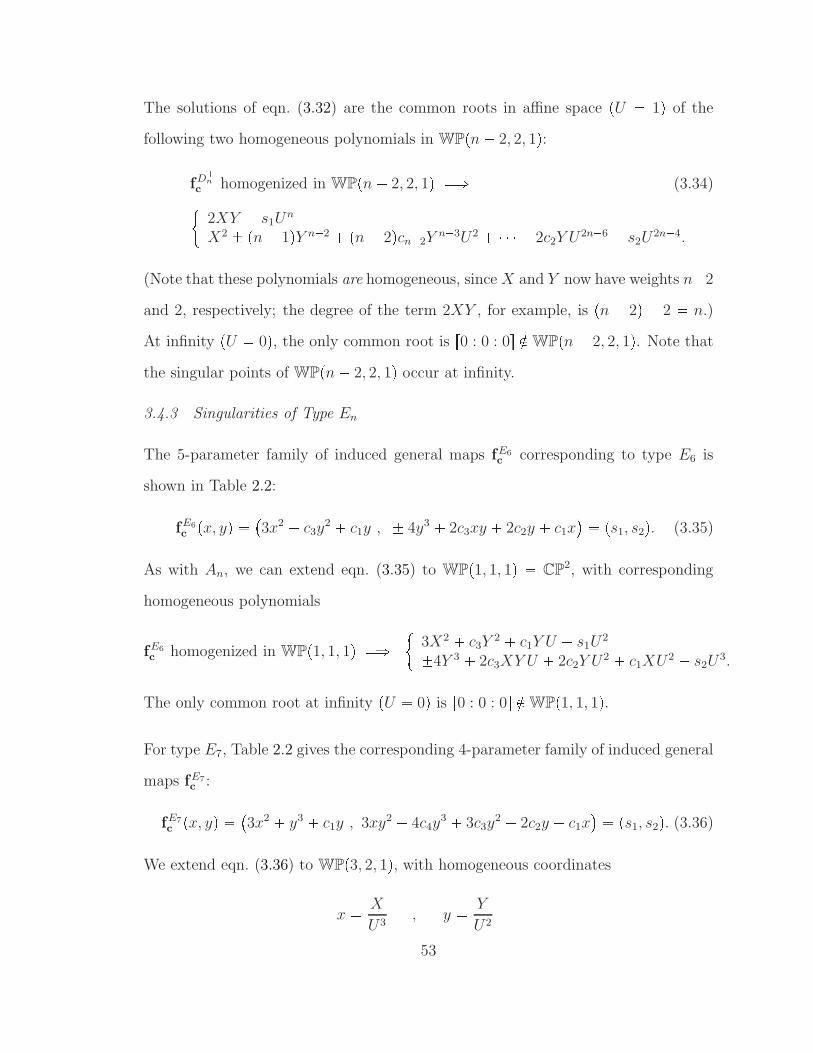
The solutions of eqn. (3.32) are the common roots in affine space pU 1q of the

following two homogeneous polynomials in WPpn 2, 2, 1q:fD

nc homogenized in WPpn 2, 2, 1q ùñ (3.34)"

2XY s1Un

X2 pn 1qY n2 pn 2qcn2Yn3U2 2c2Y U

2n6 s2U2n4.

(Note that these polynomials are homogeneous, since X and Y now have weights n2

and 2, respectively; the degree of the term 2XY , for example, is pn 2q 2 n.)

At infinity pU 0q, the only common root is r0 : 0 : 0s R WPpn 2, 2, 1q. Note that

the singular points of WPpn 2, 2, 1q occur at infinity.

3.4.3 Singularities of Type En

The 5-parameter family of induced general maps fE6c corresponding to type E6 is

shown in Table 2.2:

fE6c px, yq

3x2 c3y2 c1y , 4y3 2c3xy 2c2y c1x

ps1, s2q. (3.35)

As with An, we can extend eqn. (3.35) to WPp1, 1, 1q CP2, with corresponding

homogeneous polynomials

fE6c homogenized in WPp1, 1, 1q ùñ "

3X2 c3Y2 c1Y U s1U

24Y 3 2c3XY U 2c2Y U2 c1XU

2 s2U3.

The only common root at infinity pU 0q is r0 : 0 : 0s R WPp1, 1, 1q.For type E7, Table 2.2 gives the corresponding 4-parameter family of induced general

maps fE7c :

fE7c px, yq

3x2 y3 c1y , 3xy2 4c4y3 3c3y

2 2c2y c1x ps1, s2q. (3.36)

We extend eqn. (3.36) to WPp3, 2, 1q, with homogeneous coordinates

x X

U3, y Y

U2

53

and corresponding homogeneous polynomials

fE7c homogenized in WPp3, 2, 1q ùñ (3.37)"

3X2 Y 3 c1Y U4 s1U

6

3XY 2 4c4Y3U 3c3Y

2U3 2c2Y U5 c1XU

4 s2U7,

whose common roots in affine space pU 1q are precisely the solutions to eqn. (3.36).

The only common root at infinity pU 0q is r0 : 0 : 0s R WPp3, 2, 1q.The polynomials in this case have weighted degrees 6 and 7. As an example of

the vanishing criterion quoted in eqn. (3.29), a form ω as in eqn. (3.28) would have

vanishing sum of residues in C2 when deg h 6 7 3 2 8.

Finally, Table 2.2 gives the 5-parameter family of induced general mappings fE8c

corresponding to type E8:

fE8c px, yq

3x2 c5y3 c4y

2 c1y , 5y4 3c5xy2 2c4xy 3c3y

2 2c2y c1x ps1, s2q.

Once again we will use WPp3, 2, 1q. This time the corresponding homogeneous poly-

nomials are

fE8c homogenized in WPp3, 2, 1q ùñ (3.38)"

3X2 c5Y3 c4Y

2U2 c1Y U4 s1U

6

5Y 4 3c5XY2U 2c4XY U

3 3c3Y2U4 2c2Y U

6 c1XU5 s2U

8.

And, of course, the only common root at infinity pU 0q is r0 : 0 : 0s.3.4.4 Quantitative Forms for the Elliptic and Hyperbolic Umbilics

Elliptic and Hyperbolic Umbilics: Table 2.3 gives the universal, quantitative

form of a lensing map in the neighborhood of either an elliptic umbilic pD4 q or

hyperbolic umbilic pD4 q caustic. These are both one-parameter maps ηc induced by

54

a three-parameter time delay family Tc,s. (In the context of gravitational lensing,

c will represent some physical input, such as the source redshift.) For the elliptic

umbilic, this induced mapping is

ηc,ellpx, yq x2 y2 , 2xy 4cy

ps1, s2q,while for the hyperbolic umbilic, it is

ηc,hyppx, yq x2 2cy , y2 2cx

ps1, s2q.The desired extension in both cases is to WPp1, 1, 1q CP

2, with corresponding

homogeneous polynomials

ηc,ell homogenized in WPp1, 1, 1q ùñ "X2 Y 2 s1U

22XY 4cY U s2U2

and

ηc,hyp homogenized in WPp1, 1, 1q ùñ "X2 2cY U s1U

2

Y 2 2cXU s2U2.

The only common root at infinity pU 0q in either case is r0 : 0 : 0s R WPp1, 1, 1q.

55

4

A Lens Equation for Equatorial Kerr Black Hole

Lensing

4.1 Introduction

We now switch gears and address gravitational lensing in the setting of one of the

most important non-spherically symmetric and non-static solutions of the Einstein

equations, namely, Kerr black holes. This has already been the focus of many studies.

Indeed, several authors have explored the Kerr’s caustic structure, as well as Kerr

black hole lensing in the strong deflection limit, focusing on leading order effects

in light passing close to the region of photon capture (e.g., Rauch and Blandford

(1994), Bozza (2003, 2008a,b), Vazquez and Esteban (2003), Bozza et al. (2005),

Bozza et al. (2006), and Bozza and Scarpetta (2007)).

Studies of Kerr lensing have also been undertaken in the weak deflection limit.

In particular, Sereno and De Luca (2006, 2008) gave an analytic treatment of caus-

tics and two lensing observables for Kerr lensing in the weak deflection limit, while

Iyer and Hansen (2009a,b) found an asymptotic expression for the equatorial bending

angle. Werner and Petters (2007) used magnification relations for weak-deflection

56

Kerr lensing to address the issue of Cosmic Censorship (for lensing and Cosmic Cen-

sorship in the spherically symmetric case, see Virbhadra and Ellis (2002)).

This chapter and the next develops a comprehensive analytic framework for Kerr

black hole lensing, with a focus on regimes beyond the weak deflection limit (but not

restricted to the strong deflection limit). This chapter begins by presenting a new,

general lens equation and magnification formula governing lensing by a thin deflector.

This lens equation is applicable for non-equatorial observers and assume that the

source and observer are in the asymptotically flat region. In addition, it incorporates

the displacement for a general setting that Bozza and Sereno (2006) introduced for

the case of a spherically symmetric deflector. This occurs when the light ray’s tangent

lines at the source and observer do not intersect on the lens plane. An explicit

expression is given for this displacement when the observer is in the equatorial plane

of a Kerr black hole as well as for the case of spherical symmetry. In Chapter 5 this

lens equation is solved perturbatively to obtain analytic expressions for five lensing

observables (image positions, magnifications, total unsigned magnification, centroid,

and time delay) for the regime of quasi-equatorial lensing.

4.2 General Lens Equation with Displacement

4.2.1 Angular Coordinates on the Observer’s Sky

We assume that our deflector is a “thin lens,” by which we mean that its spatial

extent is much less than its distances to the source and observer. Let us define

Cartesian coordinates px, y, zq centered on the thin lens and oriented such that the

observer lies on the positive x-axis.

Assume that the observer in the asymptotically flat region is at rest relative to

the px, y, zq coordinates. All equations derived in this section are relative to the

asymptotically flat geometry of such an observer. The natural coordinates for the

observer to use in gravitational lensing are angles on the sky. To describe these angles,

57

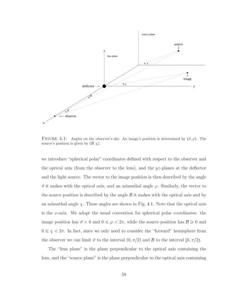
x

y

z

æ

æ

æ

ø

observer

source¯

deflector

Χ

j

J

B

­image

ô

ôô

ô

lens plane

source plane

Figure 4.1: Angles on the observer’s sky. An image’s position is determined by pϑ, ϕq. Thesource’s position is given by pB, χq.we introduce “spherical polar” coordinates defined with respect to the observer and

the optical axis (from the observer to the lens), and the yz-planes at the deflector

and the light source. The vector to the image position is then described by the angle

ϑ it makes with the optical axis, and an azimuthal angle ϕ. Similarly, the vector to

the source position is described by the angle B it makes with the optical axis and by

an azimuthal angle χ. These angles are shown in Fig. 4.1. Note that the optical axis

is the x-axis. We adopt the usual convention for spherical polar coordinates: the

image position has ϑ ¡ 0 and 0 ¤ ϕ 2π, while the source position has B ¥ 0 and

0 ¤ χ 2π. In fact, since we only need to consider the “forward” hemisphere from

the observer we can limit ϑ to the interval p0, π2q and B to the interval r0, π2q.The “lens plane” is the plane perpendicular to the optical axis containing the

lens, and the “source plane” is the plane perpendicular to the optical axis containing

58

Αï

Bæ

J

A¢

B¢

dLS

dS

dL

lens plane

­source

¯observer

image

æ

æ

Figure 4.2: A lensing scenario demonstrating that the tangent line to the segment of theray arriving at the observer and the tangent line of the ray at the source need not intersect onthe lens plane; i.e., A1 B1 in general. The angles B and ϑ are as in Fig. 4.1 (or rather, theyare their projections onto the xz-plane), α is the “bending angle,” and dL, dS , and dLS are theperpendicular distances between the lens plane and observer, the source plane and observer, andthe lens and source planes, respectively.

the source; these are also shown in Fig. 4.1. Define the distances dL and dS to be

the perpendicular distances from the observer to the lens plane and source plane,

respectively, while dLS is the perpendicular distance from the lens plane to the source

plane. Some investigators define dS to be the distance from the observer to the source

itself, as opposed to the shortest distance to the source plane. We shall comment on

this distinction in Section 4.3.3.

4.2.2 General Lens Equation via Asymptotically Flat Geometry

Consider the lensing geometry shown in Fig. 4.2. With respect to the light ray being

lensed, there are two tangent lines of interest: the tangent line to the segment of

the ray arriving at the observer and the tangent line to the ray emanating from the

source. As first emphasized in Bozza and Sereno (2006), it is important to realize

59

that these two tangent lines need not intersect. If they do intersect (as for a spherical

lens, since in that case the tangent lines are coplanar), the intersection point need

not lie in the lens plane. This effect has often been neglected, and while it may

be small in the weak deflection limit (see Section 4.3.3 below) we should include it

for greater generality. A simple way to capture this displacement is to consider the

points where the two tangent lines cross the lens plane, namely, the points A1 and

B1 in Fig. 4.2. If the tangent lines do intersect in the lens plane, then A1 B1.Otherwise, as can be seen in greater detail in Fig. 4.3, there is a displacement on the

lens plane that we quantify by defining

dy B1y A1

y , dz B1z A1

z . (4.1)

Note from Fig. 4.3 that the tangent line to the segment of the ray arriving at the

observer is determined by pϑ, ϕq. The tangent line to the ray emanating from the

source can likewise be described by the angles pϑS, ϕSq, where π2 ϑS π2 and

0 ¤ ϕS 2π. As shown in Fig. 4.3, ϑS has vertex B1 and is measured from the line

joining the points B1 and B2, which runs parallel to the optical axis. We adopt the

following sign convention for ϑS : if ϑS goes toward the optical axis, then it will be

positive; otherwise it is negative (e.g., the ϑS shown in Fig. 4.3 is positive). We will

obtain the general lens equation by considering the coordinates of the points A1 and

B1 in Fig. 4.3. Using the asymptotically flat geometry of the observer, we have

60

x

y

z

æ

æ

æ

ø

æ

æ

dL

dLSdLS

observer

source¯

deflector

Χ

j

J

JS

ô

jS

dL cos J

dL tan J

dS tan B

dLS cos JS

dLS tan JS

Νi

Ν f

A¢

B¢

B¢¢

d

ô

ô

ô

ô

ô

ô

Figure 4.3: A detailed diagram of lensing with displacement. The tangent line to the segmentof the ray arriving at the observer is determined by pϑ, ϕq and intersects the lens plane at A1, whilethe tangent line to the ray emanating from the source is determined by pϑS , ϕSq and intersects thelens plane at B1. The distance between these two points is quantified by the displacement amplituded, whose horizontal and vertical components we denote by dy and dz, respectively. The deflectorcould be a Kerr black hole and the light ray may dip below the xy-plane.

A1x 0 ,

A1y dL tanϑ cosϕ , (4.2)

A1z dL tanϑ sinϕ , (4.3)

B1x 0 ,

B1y dS tanB cosχ dLS tanϑS cospπ ϕSq , (4.4)

B1z dS tanB sinχ dLS tanϑS sinpπ ϕSq . (4.5)

61

Substituting eqns. (4.2)–(4.5) into eqn. (4.1) yields

dS tanB cosχ dL tanϑ cosϕ dLS tanϑS cosϕS dy , (4.6)

dS tanB sinχ dL tanϑ sinϕ dLS tanϑS sinϕS dz . (4.7)

The left-hand sides involve only the source position, while the right-hand sides involve

only the image position. In other words, this pair of equations is the general form

of the gravitational lens equation for source and observer in the asymptotically flat

region, for a general isolated thin lens. Note that apart from the asymptotic flatness

assumption, these equations use no properties specific to Kerr black holes; and if

the deflector was a Kerr black hole, then neither the observer nor the source was

assumed to be equatorial. We shall refer to eqns. (4.6) and (4.7), respectively, as the

“horizonal” and “vertical” components of the lens equation due to the cosine/sine

dependence on χ.

Consider now the case when the light ray and its tangent lines lie in a plane which

contains the optical axis. This forces χ ϕ or χ ϕ π depending on whether the

source is on the same or opposite side of the lens as the image. To distinguish these

two cases, it is useful to define q cospχ ϕq to be a sign that indicates whether

the source is on the same side of the lens as the image (q 1) or on the opposite

side (q 1). The condition A1 B1 will still hold in general, but the line in the

lens plane from the origin to the point B1 will now make the same angle with respect

to the y-axis as the point A1, namely, the angle ϕ (see Fig. 4.3). As a result, the

line in the source plane from the origin to the point B2 will also make the angle ϕ

with respect to the y-axis. Thus we will have ϕS ϕ π. Given these conditions,

eqns. (4.6) and (4.7) reduce to the single lens equation

dS q tanB dL tanϑ dLS tanpα ϑq d , (4.8)

where the displacement amplitude is d dycosϕ dzsinϕ (in the case of planar

rays), and to connect with traditional descriptions of gravitational lensing we have

62

introduced the light bending angle α ϑ ϑS. (If desired, the sign q can be

incorporated into the tangent so that the left-hand side is written as tanpqBq, where

we think of qB as the signed source position.) Eqn. (4.8) is the general form of

the lens equation in the case of planar rays. If the displacement d is ignored, then

eqn. (4.8) matches the spherical lens equation given by Virbhadra and Ellis (2000).

We consider the displacement term in Section 4.3.3.

4.2.3 General Magnification Formula

The magnification of a small source is given by the ratio of the solid angle subtended

by the image to the solid angle subtended by the source, since lensing conserves

surface brightness (e.g., Petters et al. (2001), p. 82). As measured by the observer,

if ℓ is the distance to the image (as opposed to the perpendicular distance), then the

small solid angle subtended by the image is

dΩI |pℓ dϑq pℓ sinϑ dϕq|ℓ2

| sinϑ dϑ dϕ| |dpcosϑq dϕ|.Similarly, the small solid angle subtended by the source is

dΩS | sinB dB dχ| |dpcosBq dχ|.We then have the absolute magnification|µ| dΩI

dΩS

| detJ |1,

where J is the Jacobian matrix

J BpcosB, χqBpcosϑ, ϕq B cosBB cos ϑB cosBBϕBχB cos ϑ

BχBϕ Writing out the determinant and dropping the absolute value in order to obtain the

signed magnification, we get

µ sinB

sin ϑ

BBBϑ BχBϕ BBBϕ BχBϑ1

. (4.9)

63

X

Y

Z

æ

æ

r cos Ζ sin Φ

r cos Ζ cos Φ

r sin Ζ

r

Φ

Ζ

Ã

ô

ò

ò

ô

Figure 4.4: Cartesian pX, Y, Zq and spherical polar pr, ζ, φq coordinates centered on the blackhole, where ζ π2 ℘ with ℘ the polar angle; note that π2 ¤ ζ ¤ π2. The black hole spinsabout the Z-axis, which corresponds to ζ π2, in the direction of increasing φ. The equatorialplane of the black hole corresponds to ζ 0 or the pX, Y q-plane.

In the case of spherical symmetry, the image and source lie in the same plane, soBBBϕ 0 and BχBϕ 1, recovering the familiar result

µ sinB

sin ϑ

BBBϑ1

.

4.3 Lens Equation for Kerr Black Holes

4.3.1 Kerr Metric

Now let the deflector in Fig. 4.3 be a Kerr black hole. The Kerr metric is the unique

axisymmetric, stationary, asymptotically flat, vacuum solution of the Einstein equa-

tions describing a stationary black hole with mass M and spin angular momentum

J (see, e.g., Wald (1984), p. 322–324). Consider the Kerr metric in Boyer-Lindquist

64

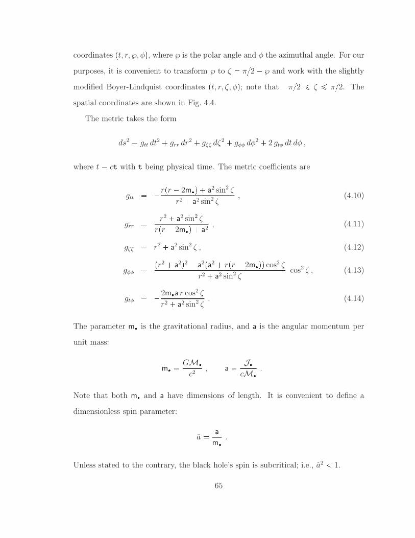
coordinates pt, r, ℘, φq, where ℘ is the polar angle and φ the azimuthal angle. For our

purposes, it is convenient to transform ℘ to ζ π2 ℘ and work with the slightly

modified Boyer-Lindquist coordinates pt, r, ζ, φq; note that π2 ¤ ζ ¤ π2. The

spatial coordinates are shown in Fig. 4.4.

The metric takes the form

ds2 gtt dt2 grr dr

2 gζζ dζ2 gφφ dφ

2 2 gtφ dt dφ ,

where t ct with t being physical time. The metric coefficients are

gtt rpr 2m q a2 sin2 ζ

r2 a2 sin2 ζ, (4.10)

grr r2 a2 sin2 ζ

rpr 2m q a2, (4.11)

gζζ r2 a2 sin2 ζ , (4.12)

gφφ pr2 a2q2 a

2pa2 rpr 2m qq cos2 ζ

r2 a2 sin2 ζcos2 ζ , (4.13)

gtφ 2m a r cos2 ζ

r2 a2 sin2 ζ. (4.14)

The parameter m is the gravitational radius, and a is the angular momentum per

unit mass:

m GM c2

, a J cM .

Note that both m and a have dimensions of length. It is convenient to define a

dimensionless spin parameter:

a a

m .Unless stated to the contrary, the black hole’s spin is subcritical; i.e., a2 1.

65

4.3.2 Lens Equation for an Equatorial Observer

We now specialize to the case when the observer lies in the equatorial plane of the

Kerr black hole, so the coordinates px, y, zq in Fig. 4.2 coincide with the coordinatespX, Y, Zq in Fig. 4.4. Note that we still consider general source positions.

In Appendix 4.4 we carefully analyze null geodesics seen by an observer in the

equatorial plane. By considering constants of the motion, we derive the following

lens equation:

dS tanB cosχ dLS tanϑS cosϕS dL

sin ϑ cosϕ

cos ϑS

, (4.15)

dS tanB sinχ dLS tanϑS sinϕS dL sinϑ

1 sin2 ϑS sin2 ϕS

(4.16)cosϕ sinϑS tanϑS sinϕS cosϕS

sin2 ϕ sin2 ϑS sin2 ϕS

12.

This is the general form of the lens equation for an equatorial observer in the Kerr

metric for observer and source in the asymptotically flat region. It is valid for all

light rays, whether they loop around the black hole or not, as long as they lie outside

the region of photon capture. No small-angle approximation is required.

Note that eqns. (4.6) and (4.7) represent the general form of the lens equation,

with the displacement terms explicitly written, while eqns. (5.3) and (5.4) give the

exact lens equation for an equatorial Kerr observer, with the displacement terms

implicitly included. Demanding that these two pairs of equations be equivalent

allows us to identify the displacement terms for an equatorial Kerr observer:

dy dL sinϑ cosϕ

1

cos ϑS

1

cosϑ

, (4.17)

dz dL tanϑ sinϕ dL sinϑ

1 sin2 ϑS sin2 ϕS

cosϕ sinϑS tanϑS sinϕS cosϕS

sin2 ϕ sin2 ϑS sin2 ϕS

12. (4.18)

66

4.3.3 Schwarzschild Case

In the case of a spherically symmetric lens we have ϕS ϕ π, and either χ ϕ

or χ ϕ π, depending on whether the source lies on the same or opposite side

of the lens as the image. Once again, we define q cospχ ϕq to be a sign that

distinguishes these two cases. With these conditions eqns. (5.3) and (5.4) combine

to form the single lens equation with displacement for a Schwarzschild black hole:

dS q tanB dL

sinϑ

cosϑS

dLS tanϑS . (4.19)

Two comments are in order. First, our spherical lens equation (4.19) is equivalent

to the spherical lens equation recently derived by Bozza and Sereno (2006) (up to

the sign q, which was not discussed explicitly in Bozza and Sereno (2006)); see also

Bozza (2008a). The second comment refers to the amplitude of the displacement.

By comparing our general planar-ray lens equation (4.8) with eqn. (4.19), we can

identify the displacement

d dL sinϑ

1

cospα ϑq 1

cosϑ

, (4.20)

where we have switched from ϑS to the bending angle α ϑ ϑS. Now let δα αmod 2π, and assume that ϑ and δα are small. (Note that we need not assume α

itself is small, only that δα is small. This means that our analysis applies to all light

rays, including those that loop around the lens.) Taylor expanding the displacement

in ϑ and α yields

d dL

2pϑ δαqpδα 2ϑq Op4q.

4.4 Exact Kerr Null Geodesics for Equatorial Observers

In this section we determine the equations of motion governing light rays seen by

equatorial observers in the Kerr metric. We obtain the exact equations of motion by

67

considering constants of the motion.

4.4.1 Equations of Motion for Null Geodesics

We first study the equations of motion for a general Kerr null geodesic Cpλq ptpλq, rpλq, ζpλq, φpλqq, where λ is an affine parameter. The geodesic is assumed to

be outside the region of photon capture. Two immediate constants of the motion for

Kerr geodesics are the energy E and the orbital angular momentum L. They yield

two equations of motion (see, e.g., O’Neill (1995), p. 180):9t gφφE gtφL

g2tφ gttgφφ

,9φ gtφE gttL

gttgφφ g2tφ

,

where the dot denotes differentiation relative to the affine parameter λ. Since we

only consider unbound light rays, we may assume E ¡ 0. With a suitable fixed choice

of affine parameter λ, we henceforth assume that E λ has dimension of length. The

dimension of the ratio LE is also length. A third constant of motion is nullity, which

yields 9r gtt9t2 gζζ

9ζ2 gφφ9φ2 2gtφ

9t 9φgrr

12.

A fourth constant of motion Q is the Carter constant, which comes from separating

the Hamilton-Jacobi equation (Carter (1968)). We henceforth assume that Q ¥ 0;

i.e., that the light ray either crosses the equatorial plane or asymptotically approaches

it (see, e.g., O’Neill (1995), p. 204–205). Employing the notation

λ E λ , 9x dx

dλ, L L

E, Q Q

E2,

68

the fourth equation of motion can be written9ζ dζ

dλ pQ a

2 sin2 ζ L2 tan2 ζq12r2 a2 sin2 ζ

. (4.21)

Using the metric coefficients (4.10)–(4.14) shown in Section 4.3.1, the null geodesic

equations of motion become9t 1 2m rpa2 aL r2qra2 rpr 2m qspr2 a2 sin2 ζq , (4.22)9r rr4 pQ L2 a2qr2 2m ppL aq2 Qqr a

2Qs12r2 a2 sin2 ζ

, (4.23)9φ 2am r Lrpr 2m q sec2 ζ a2L tan2 ζra2 rpr 2m qspr2 a2 sin2 ζq . (4.24)

Eqns. (4.21)–(4.24) form the set of equations of motion that we must solve in order

to describe null geodesics in the Kerr metric.

4.4.2 Exact Lens Equation for Equatorial Observers

Assuming that the source and equatorial observer are in the asymptotically flat

region, we consider now the constants of motion L and Q. We can find them by

examining the equations of motion in the asymptotically flat region of the spacetime

far from the black hole. Formally, this means taking the limits a,m Ñ 0, in which

case the equations of motion reduce to9t 1 , 9r pr2 Q L2q12r

, 9ζ pQ L2 tan2 ζq12r2

, 9φ L

r2 cos2 ζ.

(4.25)

At the position of the observer, the light ray is a straight line described by the angles

ϑ and ϕ. For an equatorial observer, we see from Fig. 4.3 that the three Cartesian

69

components of the line can be written as

xpλq dL pλ λOq cosϑ ,

ypλq pλ λOq sinϑ cosϕ ,

zpλq pλ λOq sinϑ sinϕ ,

where λO is the value of the affine parameter at the position of the observer, and

the affine parameter range for the line segment is dLcos ϑ λO ¤ λ ¤ λO (recall

that 0 ϑ π2 and that λ has dimension of length). Next, we convert to spherical

coordinates pr, ζ, φq and evaluate r, ζ , 9r, and 9φ at λ λO:

rpλOq dL , ζpλOq 0 , 9r pλOq cosϑ , 9φ pλOq sin ϑ cosϕ

dL

. (4.26)

Finally, we substitute eqn. (4.26) into eqn. (4.25) to solve for L and Q when λ λO:

LO 9φ r2 cos2 ζλλO

dL sinϑ cosϕ , (4.27)

QO r21 9r 2

L2

λλO

d2L sin2 ϑ sin2 ϕ . (4.28)

(To be clear, we have labeled these constants of motion with “O” for observer. Note

that QO ¥ 0. Note also that we could just as well have used 9r and 9ζ , or 9ζ and 9φ, to

solve for L and Q.) Going further, we define

b Q L2

12 dL sinϑ (4.29)

to be the (absolute) impact parameter of the light ray (since 0 ϑ π2, sinϑ is

positive.) This is clearly a constant of the motion.

We could equally well express the constants of motion in terms of the light ray at

the position of the source. To be clear, we write these constants as LS and QS. Recall

that the position of the source is defined by the angles pB, χq, while the direction of

70

the light ray at the source is defined by the angles pϑS, ϕSq. So the three Cartesian

components of the light ray at the source can be written as

xpλq dLS pλ λSq cosϑS ,

ypλq dS Ysrc pλ λSq sinϑS cosϕS ,

zpλq dS Zsrc pλ λSq sinϑS sinϕS ,

where λS is the value of the affine parameter at the position of the source, and the

affine parameter range for the line segment is λS ¤ λ ¤ dLScos ϑS λS (recall that

0 ¤ ϑS π2). Note that for simplicity we have defined

Ysrc tanB cosχ , Zsrc tanB sinχ .

By a computation identical to those in eqns. (4.26) and (4.28), we solve eqn. (4.25)

for L and Q when λ λS to obtain

LS dS Ysrc cos ϑS dLS sinϑS cosϕS , (4.30)

QS d2SZ

2srcpcos2 ϑS sin2 ϑS cos2 ϕSq2 dS Zsrc sin ϑS sinϕSpdLS cosϑS dS Ysrc sinϑS cosϕSqpd2SY

2src d2

LSq sin2 ϑS sin2 ϕS . (4.31)

Since we are discussing constants of the motion, we must have LO LS and QO QS. Using eqns. (4.27) and (4.30), the condition LO LS is a trivial linear equation

for Ysrc, which yields

dS tanB cosχ dLS tanϑS cosϕS dL

sinϑ cosϕ

cosϑS

. (4.32)

Using eqns. (4.28) and (4.31), the condition QO QS is a quadratic equation in Zsrc,

71

which yields the following two roots:

Zsrc dLS tanϑS sinϕS

dS

dL sin ϑ

dS

1 sin2 ϑS sin2 ϕS

(4.33)cosϕ sinϑS tanϑS sinϕS cosϕS

sin2 ϕ sin2 ϑS sin2 ϕS

12.

We will take the positive root in eqn. (4.33) because in the case of spherical sym-

metry only the positive root, taken together with eqn. (4.32), will combine to form

eqn. (4.19) in Section 4.3.3. We thus have

dS tanB sinχ dLS tanϑS sinϕS dL sinϑ

1 sin2 ϑS sin2 ϕS

(4.34)cosϕ sinϑS tanϑS sinϕS cosϕS

sin2 ϕ sin2 ϑS sin2 ϕS

12.

Eqns. (4.32) and (4.34) thus constitute the two components of the general lens equa-

tion for an equatorial observer in the Kerr metric.

72

5

Quasi-Equatorial Lensing Observables

5.1 Introduction

This last chapter addresses lensing observables in the regime of quasi-equatorial

lensing by a Kerr black hole. First, the full light bending angle is obtained with

“horizontal” and “vertical” components for an equatorial observer and light rays that

are quasi-equatorial. Next, the lens equation of Chapter 5 is solved perturbatively to

second order in ε, which is the ratio of the angular gravitational radius to the angular

Einstein radius, to obtain formulas for the lensing observables: image position, image

magnification, total unsigned magnification, centroid, and time delay. It is shown

that the displacement begins to affect the lensing observables only at second order in

ε, and so can safely be ignored for studies of first-order corrections to weak-deflection

quasi-equatorial Kerr lensing. The findings presented here also yield new results on

the lensing observables in Schwarzschild lensing with displacement.

5.2 Definitions and Assumptions

We work under the following assumptions:

73

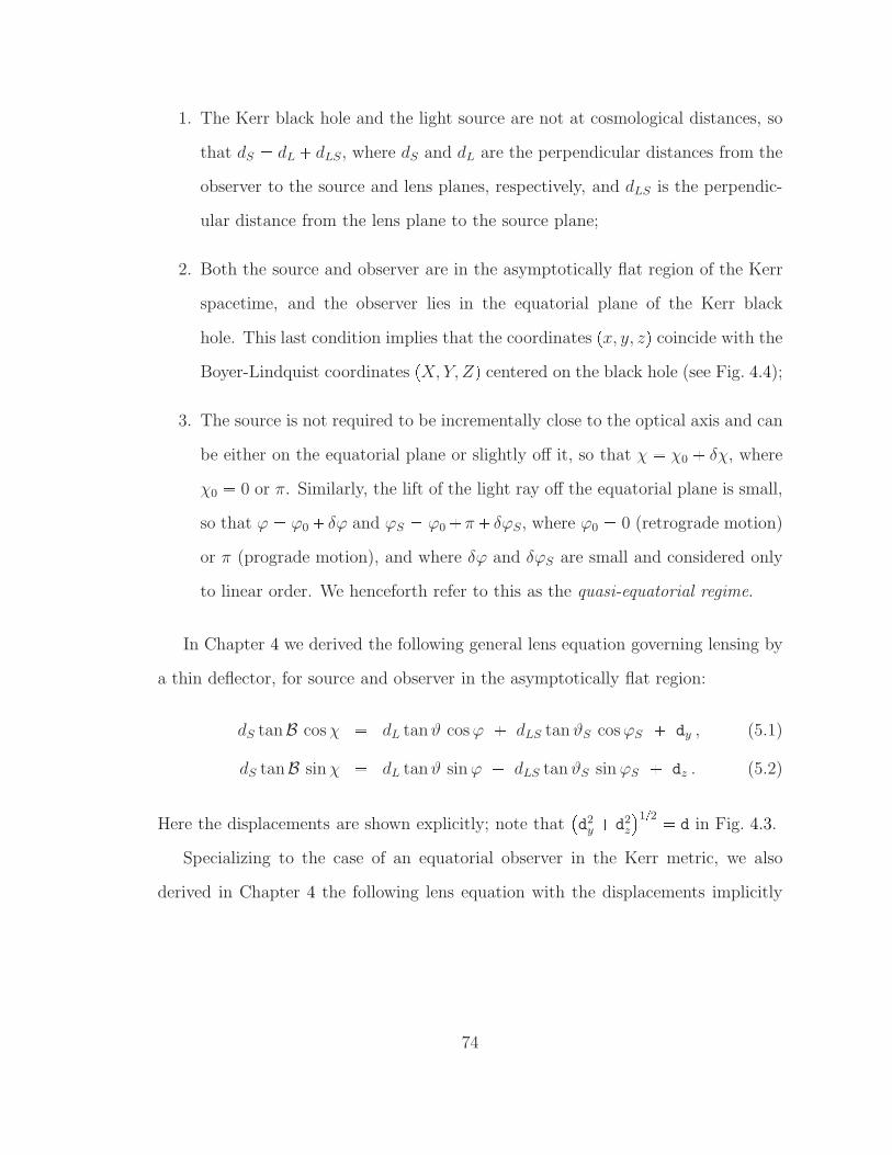
1. The Kerr black hole and the light source are not at cosmological distances, so

that dS dL dLS, where dS and dL are the perpendicular distances from the

observer to the source and lens planes, respectively, and dLS is the perpendic-

ular distance from the lens plane to the source plane;

2. Both the source and observer are in the asymptotically flat region of the Kerr

spacetime, and the observer lies in the equatorial plane of the Kerr black

hole. This last condition implies that the coordinates px, y, zq coincide with the

Boyer-Lindquist coordinates pX, Y, Zq centered on the black hole (see Fig. 4.4);

3. The source is not required to be incrementally close to the optical axis and can

be either on the equatorial plane or slightly off it, so that χ χ0 δχ, where

χ0 0 or π. Similarly, the lift of the light ray off the equatorial plane is small,

so that ϕ ϕ0 δϕ and ϕS ϕ0π δϕS, where ϕ0 0 (retrograde motion)

or π (prograde motion), and where δϕ and δϕS are small and considered only

to linear order. We henceforth refer to this as the quasi-equatorial regime.

In Chapter 4 we derived the following general lens equation governing lensing by

a thin deflector, for source and observer in the asymptotically flat region:

dS tanB cosχ dL tanϑ cosϕ dLS tanϑS cosϕS dy , (5.1)

dS tanB sinχ dL tanϑ sinϕ dLS tanϑS sinϕS dz . (5.2)

Here the displacements are shown explicitly; note thatd2

y d2z

12 d in Fig. 4.3.

Specializing to the case of an equatorial observer in the Kerr metric, we also

derived in Chapter 4 the following lens equation with the displacements implicitly

74

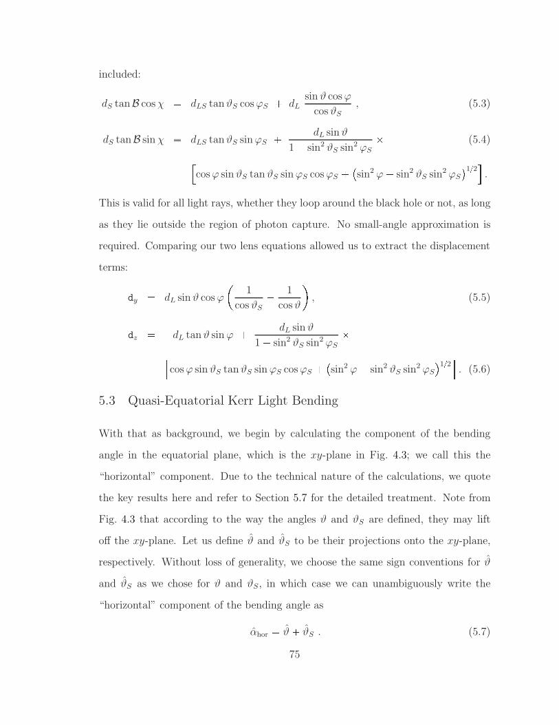
included:

dS tanB cosχ dLS tanϑS cosϕS dL

sin ϑ cosϕ

cos ϑS

, (5.3)

dS tanB sinχ dLS tanϑS sinϕS dL sinϑ

1 sin2 ϑS sin2 ϕS

(5.4)cosϕ sinϑS tanϑS sinϕS cosϕS

sin2 ϕ sin2 ϑS sin2 ϕS

12.

This is valid for all light rays, whether they loop around the black hole or not, as long

as they lie outside the region of photon capture. No small-angle approximation is

required. Comparing our two lens equations allowed us to extract the displacement

terms:

dy dL sinϑ cosϕ

1

cos ϑS

1

cosϑ

, (5.5)

dz dL tanϑ sinϕ dL sinϑ

1 sin2 ϑS sin2 ϕS

cosϕ sinϑS tanϑS sinϕS cosϕS

sin2 ϕ sin2 ϑS sin2 ϕS

12. (5.6)

5.3 Quasi-Equatorial Kerr Light Bending

With that as background, we begin by calculating the component of the bending

angle in the equatorial plane, which is the xy-plane in Fig. 4.3; we call this the

“horizontal” component. Due to the technical nature of the calculations, we quote

the key results here and refer to Section 5.7 for the detailed treatment. Note from

Fig. 4.3 that according to the way the angles ϑ and ϑS are defined, they may lift

off the xy-plane. Let us define ϑ and ϑS to be their projections onto the xy-plane,

respectively. Without loss of generality, we choose the same sign conventions for ϑ

and ϑS as we chose for ϑ and ϑS, in which case we can unambiguously write the

“horizontal” component of the bending angle as

αhor ϑ ϑS . (5.7)

75

Note that the positivity of ϑ and the fact that the bending angle is nonnegative

forces the condition

ϑS ¥ ϑ .(Indeed, with our signs conventions the condition ϑS ϑ would be equivalent to

repulsion of the light ray.) Writing ϑ and ϑS in terms of the angles ϑ, ϕ, ϑS, ϕS, we

have

ϑ tan1ptanϑ cosϕq , (5.8)

ϑS tan1ptanϑS cospπ ϕSqq . (5.9)

As stated in assumption (3) above, in the quasi-equatorial regime we have

ϕ ϕ0 δϕ , ϕS ϕ0 π δϕS , (5.10)

where ϕ0 is either 0 (retrograde motion) or π (prograde motion), while δϕ and δϕS

are small and considered only to linear order. In this regime eqns. (5.8) and (5.9)

simplify to

ϑ ϑ ,ϑS ϑS .

Since ϑ and ϑS have the same signs as ϑ and ϑS, respectively, we discard the negative

solutions, so that eqn. (5.7) reduces to

αhor ϑ ϑS , ϑS ¥ ϑ . (5.11)

Thus in the quasi-equatorial regime we may use the full angles ϑ and ϑS in place of

their respective projections onto the xy-plane. With that said, we show in eqn. (5.70)

of Section 5.7 that the “horizontal” bending of light has the following invariant series

expansion:

αhorpbq A1

m b

A2

m b

2 A3

m b

3 A4

m b

4 O

m b

5

,

(5.12)

76

where

A1 4 , (5.13)

A2 15π

4 4 s a , (5.14)

A3 128

3 10 π s a 4 a2 , (5.15)

A4 3465π

64 192 s a 285π a2

16 4 s a3 . (5.16)

The variable s equals 1 depending on whether the light ray undergoes progradep1q or retrograde p1q motion (see eqn. (5.57) in Section 5.7 below). Note that

eqns. (5.12)–(5.16) are consistent with the bending angle obtained by Iyer & Hansen

Iyer and Hansen (2009a) by a different means—note also that their bending angle

is consistent with the exact bending angle Iyer and Hansen (2009a,b). We remind

the reader of our conventions in Chapter 4. The parameter m is the gravitational

radius and a is the angular momentum per unit mass,

m GM c2

, a J cM , (5.17)

where M is the mass of the black hole and J its spin angular momentum (see,

e.g., Wald (1984), pp. 322–324). Note that both m and a have dimensions of length.

The quantity a is a dimensionless spin parameter:

a a

m .Unless stated to the contrary, the black hole’s spin is subcritical; i.e., a2 1. Finally,

b dL sinϑ is the impact parameter (see eqn. (4.29) in Chapter 4), which is a

constant of the motion.

When there is no spin, the coefficients reduce to A1 4, A2 15π4, A3 1283,

A4 3465π64 and recover the Schwarzschild bending angle in Keeton and Petters

77

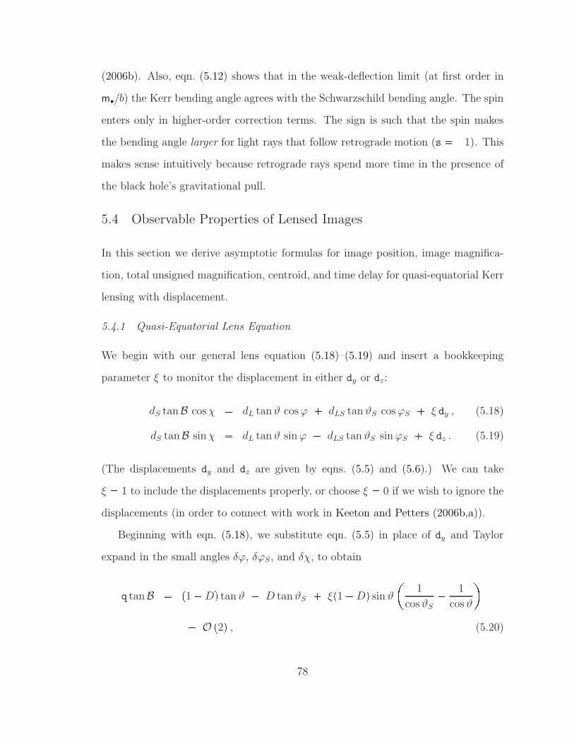
(2006b). Also, eqn. (5.12) shows that in the weak-deflection limit (at first order in

m b) the Kerr bending angle agrees with the Schwarzschild bending angle. The spin

enters only in higher-order correction terms. The sign is such that the spin makes

the bending angle larger for light rays that follow retrograde motion (s 1). This

makes sense intuitively because retrograde rays spend more time in the presence of

the black hole’s gravitational pull.

5.4 Observable Properties of Lensed Images

In this section we derive asymptotic formulas for image position, image magnifica-

tion, total unsigned magnification, centroid, and time delay for quasi-equatorial Kerr

lensing with displacement.

5.4.1 Quasi-Equatorial Lens Equation

We begin with our general lens equation (5.18)–(5.19) and insert a bookkeeping

parameter ξ to monitor the displacement in either dy or dz:

dS tanB cosχ dL tanϑ cosϕ dLS tanϑS cosϕS ξ dy , (5.18)

dS tanB sinχ dL tanϑ sinϕ dLS tanϑS sinϕS ξ dz . (5.19)

(The displacements dy and dz are given by eqns. (5.5) and (5.6).) We can take

ξ 1 to include the displacements properly, or choose ξ 0 if we wish to ignore the

displacements (in order to connect with work in Keeton and Petters (2006b,a)).

Beginning with eqn. (5.18), we substitute eqn. (5.5) in place of dy and Taylor

expand in the small angles δϕ, δϕS, and δχ, to obtain

q tanB p1Dq tanϑ D tanϑS ξp1Dq sinϑ 1

cosϑS

1

cosϑ

O p2q , (5.20)

78

where q cospχ0 ϕ0q, D dLSdS, and O p2q indicates terms that are second

order in δϕ, δϕS, and/or δχ. (Below, we incorporate the sign q into the tangent

so that the left-hand side is written as tanpqBq and we think of qB as the signed

source position.) This is the “horizontal” component of the lens equation. Recall

that ξ identifies terms associated with the displacement. Including the displacement

by setting ξ 1 in eqn. (5.20) yields

q tanB p1Dq sinϑ

cosϑS

D tanϑS O p2q .Thus, to lowest order in out-of-plane motion we recover the same lens equation as in

the Schwarzschild case (see eqn. (4.19) in Chapter 4).

We use ϑS αhorϑ, taking αhor from eqn. (5.12), and introduce scaled angular

variables:

β qB

ϑE

, θ ϑ

ϑE

, ϑ tan1

m dL

, ε ϑ

ϑE

ϑE

4D. (5.21)

Here the natural angular scale is given by the angular Einstein ring radius:

ϑE 4GM dLS

c2dLdS

4m DdL

. (5.22)

Note that we have defined the scaled source position β to be a signed quantity, with

a sign that indicates whether the source is on the same or opposite side of the lens

as the image. In eqn. (5.12) we wrote the bending angle αhor as a series expansion in

m b. For analyzing the observable image positions, ε is the more natural expansion

parameter. To convert αhor into a series expansion in ε, note that according to

eqns. (5.21) and (5.22) and the fact that b dL sinϑ, we have

m b 4D ε2

sinp4D ε θq 1

θε 8D2 θ

3ε3 O pεq5 . (5.23)

79

As in Keeton and Petters (2006b,a, 2005), we postulate that the solution of the

“horizontal” lens equation (5.20) can be written as a series expansion of the form

θ θ0 θ1 ε θ2 ε2 O pεq3 . (5.24)

Converting now to our scaled angular variables (5.21)–(5.24), our quasi-equatorial

“horizontal” lens equation (5.20) takes the form

β θ0 1

θ0

1

θ20

s a 15π

16 p1 θ2

0q θ1 ε (5.25) 1

24 θ30

12 s a p5π 4θ1q 24 a2 384 3 θ1 p15π 8θ1q 24 θ0 θ2 p1 θ2

0q 8 θ048D θ0 8D2 θ2

0p2β3 7θ0 2θ30q 192θ2

0 p1Dqp1 2D θ20q ξ ε2 O pεq3 .

Note that displacement terms (indicated by ξ) only begin to appear at second or-

der. Also, since we are simultaneously expanding tan qB tanp4 β D εq, note the

occurrence of β3 in the ε2 term.

Now we turn to the “vertical” component of the lens equation, namely, eqn. (5.19).

Substituting eqn. (5.6) in place of dz and Taylor expanding in the small angles δϕ,

δϕS, and δχ, we obtainpδχq pq tanBq pδϕq p1 ξqp1Dq tanϑ pδϕSqD tanϑS (5.26) ξp1Dq sinϑ!pδϕS sin ϑS tanϑS pδϕq2 pδϕSq2 sin2 ϑS

12) O p2q .Next, we use eqn. (5.79) in Section 5.7 to write pδϕSq sinϑS pδϕqW pϑq:pδχq pq tanBq δϕ p1 ξqp1Dq tanϑ δϕDW pϑqpcosϑSq1 (5.27) ξp1Dq sinϑtδϕW pϑq tanϑS δϕ r1W pϑq2s12u .

80

(In Section 5.7 we show that 1W pϑq2 ¡ 0, so this equation is never complex-valued.)

Finally, we convert to our scaled angular variables (5.21)–(5.24) and expand in ε,

obtainingβ 16

3D2 β3 ε2 O pεq4 δχ

δϕ

"θ0 1

θ0

1

θ20

2 s a 15π

16 p1 θ2

0q θ1 ε 1

24 θ30

s a p90π 96θ1q 2a2 45πθ1 24p16 θ2

1q 8θ08D2θ3

0p7 2θ20 6ξq 3pθ2 θ2

0θ2 8θ0ξq 24Dθ0p2 ξ 2θ20ξqε2 O pεq3+ . (5.28)

This is the “vertical” component of the lens equation. We will use it to obtain a

relation between the small angles δχ and δϕ. To that end, we divide eqn. (5.28) by

eqn. (5.25) to eliminate β:

δχ δϕ

#1 s a

θ0pθ20 1q ε (5.29) a

16θ20pθ2

0 1q2s p5π 4θ20p5π 12θ1q 16θ1q 16ap1 2θ2

0qε2 O pεq3+.Observe that in general δχ δϕ in the regime of quasi-equatorial lensing. Thus

when a 0, the light ray’s trajectory cannot lie in a plane other than the equatorial

plane (in which case δϕ δχ 0).

5.4.2 Image Positions

We now solve our “horizontal” lens equation (5.25) term by term to find θ0, θ1, θ2,

and θ3. The zeroth-order term is the familiar weak-deflection lens equation for the

81

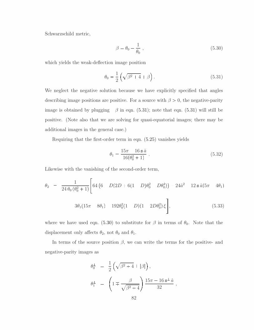
Schwarzschild metric,

β θ0 1

θ0, (5.30)

which yields the weak-deflection image position

θ0 1

2

aβ2 4 β

. (5.31)

We neglect the negative solution because we have explicitly specified that angles

describing image positions are positive. For a source with β ¡ 0, the negative-parity

image is obtained by plugging β in eqn. (5.31); note that eqn. (5.31) will still be

positive. (Note also that we are solving for quasi-equatorial images; there may be

additional images in the general case.)

Requiring that the first-order term in eqn. (5.25) vanishes yields

θ1 15π 16 s a

16pθ20 1q . (5.32)

Likewise with the vanishing of the second-order term,

θ2 1

24 θ0 pθ20 1q64

6Dp2D 6p1Dqθ2

0 Dθ40q 24a2 12 s ap5π 4θ1q3θ1p15π 8θ1q 192θ2

0p1Dqp1 2Dθ20q ξ, (5.33)

where we have used eqn. (5.30) to substitute for β in terms of θ0. Note that the

displacement only affects θ2, not θ0 and θ1.

In terms of the source position β, we can write the terms for the positive- and

negative-parity images as

θ0 1

2

aβ2 4 |β| ,

θ1 1 |β|a

β2 4

15π 16 s a

32,

82

where we have written s to remind ourselves that the two images have different

respective values of the prograde/retrograde sign parameter. In fact, we have s s. The terms θ2 as functions of β are similarly obtained, but are too lengthy to be

written here. Now thinking of the universal relations studied in Keeton and Petters

(2006a), we observe that the zeroth-order terms obey

θ0 θ0 |β|, θ0 θ0 1,

which are identical to the zeroth-order position relations obeyed by PPN models (see

Keeton and Petters (2006a)). The first-order terms have

θ1 θ1 15π

16 s a |β|a

β2 4.

In Keeton and Petters (2006a) it was shown that θ1 θ1 is independent of source

position for static, spherical black holes in all theories of gravity that can be expressed

in the PPN framework. However, as first shown in Werner and Petters (2007), we

see that in the presence of spin, θ1 θ1 is no longer independent of source position.

This is a direct consequence of the fact that one image corresponds to a light ray

that follows prograde motion, while the other has retrograde motion. The difference

between the second-order components is (cf. Keeton and Petters (2006a))

θ2 θ2 2a2a

4 β2 a|β|p16a 15πsqa4 β2

8p4 β2q32 30πsa ap48a 15πsq p4 β2q8 p4 β2q32 |β| I

256,

where

I 4096 225π2 2048D2 160πsa 512a2 4096Dp1Dqξ.Plots of the image correction terms θ1 and θ2 as functions of the source position β are

shown in Fig. 5.1, for a positive-parity image undergoing either prograde ps 1qor retrograde ps 1q motion.

83

0.2 0.5 0.8 1.1 1.40.4

0.6

0.8

1.0

1.2

1.4

Β Hin units of JEL

Schwarzschild

Kerr Hs = +1L

Kerr Hs = -1L

Θ1

0.2 0.5 0.8 1.1 1.4

1

2

3

4

5

Β Hin units of JEL

Kerr Hs = +1L

Kerr Hs = -1L

Schwarzschild

Θ2

Figure 5.1: First- and second- order angular image correction terms as functions of the angularsource position β, for a positive-parity image undergoing either prograde ps 1q or retrogradeps 1q motion near the equatorial plane of a Kerr black hole. The solid curves represent a Kerrblack hole with spin parameter a 0.7. When a 0, we recover Schwarzschild lensing (dashedcurves). For the second- and third- order image corrections, the displacement parameter ξ 1and D dLSdS 0.5. (Note that θ1 and θ2 are dimensionless, but have factors of ε and ε2,respectively. Note also that dLS and dS are the perpendicular distances between the lens andsource planes and the observer and source plane, respectively.) These results hold for a black holewith sufficiently small ϑE .

5.4.3 Magnifications

In Chapter 4 we derived the following general magnification formula:

µ sinB

sin ϑ

BBBϑ BχBϕ BBBϕ BχBϑ1

. (5.34)

To compute BBBϑ, we employ the same techniques that led to eqn. (5.25). ForBχBϕ, we use eqn. (5.29). (Note that BBBϕ 0 for quasi-equatorial lensing.) The

result is the following series expansion:

µ µ0 µ1 ε µ2 ε2 O pεq3 , (5.35)

84

where

µ0 θ40

θ40 1

, (5.36)

µ1 r15πpθ20 1q2 64 s a θ2

0s θ30

16 pθ20 1q2pθ2

0 1q3 , (5.37)

µ2 θ20

384pθ20 1q3pθ2

0 1q5768 a2θ40p5 2θ2

0 5θ40q (5.38) 120πsap1 16θ2

0 34θ40 44θ6

0 39θ80 12θ10

0 q θ20pθ2

0 1q2 12288Dpθ0 θ30q2 1024D2p1 θ2

0q2pθ40 16θ2

0 1q 3θ20

4096 θ2

0p675π2 4096pθ20 2qq 6144pD 1q θ0 θ5

0q2p1 2Dθ20p2 θ2

0q ξ .

Note that displacement terms (indicated by ξ) begin to appear only at second order

in ε. In terms of the source position β, we can write the terms for the positive- and

negative-parity images as

µ0 1

2 β2 2

2 |β|aβ2 4,

µ1 15π β2 64 s a16 β2 pβ2 4q32 ,

µ2 2025π2 1024pβ2 4qp12Dp12 pβ2 18qDqq384 |β| pβ2 4q52 5π s a

32 β2

1 |β| pβ4 34β2 48qpβ2 4q52 2 a2 5β2 8|β|3pβ2 4q52 16 ξ p1Dq D Dpβ4 6β2 6q 1|β| pβ2 4q32 .

85

Observe that

µ0 µ0 1 ,

µ0 µ0 β2 2|β| pβ2 4q12 ,µ1 µ1 15π

8pβ2 4q32 ,µ1 µ1 8 s a

β2pβ2 4q32 ,µ2 µ2 5π s a

16

|β| pβ4 34β2 48qβ2pβ2 4q52 32 ξ Dp1Dq ,

µ2 µ2 5π s a16 β2

4 a2 5β2 8|β|3pβ2 4q52 (5.39) 32 ξ p1Dq Dpβ4 6β2 6q 1|β| pβ2 4q32 2025π2 1024pβ2 4qp12Dp12 pβ2 18qDqq192 |β| pβ2 4q52 .

The zeroth-order sum relation is the same as the universal relation found for static,

spherical PPN models in Keeton and Petters (2006a). Notice that the zeroth-order

difference relation is independent of spin. In the first-order difference relation, the

right-hand side is zero for PPN models, but nonzero in the presence of spin (see also

Werner and Petters (2007)). In the second-order sum relation, the right-hand side

is not zero even in the absence of spin. This is a consequence of the displacement

(indicated by ξ).

5.4.4 Critical and Caustic Points

To determine the set of critical points, we set µ1 0, the reciprocal of the series

expansion given by eqn. (5.35) in Section 5.4.3, and solve for θ0, θ1, θ2, and θ3 (see

Aazami et al. (2011a) for a derivation of the third-order term θ3). This yields the

86

following θ-components:

θ0critical

1 , (5.40)

θ1critical

s a 15π

32, (5.41)

θ2critical

8 15π s a

32 675π2

2048D2

20

3 8 ξ

4Dp3 ξ 2q 4ξ , (5.42)

θ3critical

s a 225π2

256 8D2 p1 ξq 8D ξ 8

15π a2

64(5.43) 15πp400 225π2 4096D2p1 ξq 2048 ξ 2048Dp2 3 ξqq

8192,

where “ ” corresponds to the two values s 1. Note that since we are in the

regime of quasi-equatorial Kerr lensing (ϕ ϕ0δϕ with ϕ0 0 (retrograde motion)

or π (prograde motion)), eqns. (5.40)–(5.43) do not define a circle on the lens plane,

but are to be interpreted (by eqn. (5.58)) as four points pθcrit, π δϕq, pθcrit,δϕqon the lens plane, for a given δϕ. We now insert these into the “horizontal” lens

equation (5.25) to third order in ε and solve for β. This yields the β-components of

the caustic points, which we express here as a series expansion in ε to third order:

βcaustic

s a ε 5π s a

16ε2 (5.44) a

512

1136π a s

225π2 4096 ξ 4096D2p1 2ξq 4096Dp2 3ξq ε3O pεq4 ,

The signs correspond to prograde (s 1) and retrograde (s 1) motion,

respectively. When a 0 the two caustic points converge to one point at the origin

of the source plane. Note from the third-order term that the caustic points are not

symmetric about the vertical axis on the light source plane.

87

5.4.5 Total Magnification and Centroid

If the two images are too close together to be resolved (as in microlensing), the main

observables are the total unsigned magnification and the magnification-weighted cen-

troid position. Using our results above, we compute the total unsigned magnification:

µtot |µ| |µ| β2 2|β| pβ2 4q12 8 s aβ2pβ2 4q32 ε (5.45) pµ2 µ2 q ε2 O pεq3 ,

where the second-order term is given by eqn. (5.39). The magnification-weighted

centroid position (actually, its “horizontal” component, since we are in the regime of

quasi-equatorial lensing) is

Θcent θ|µ| θ|µ||µ| |µ| |β| pβ2 3qβ2 2

p2 β2q s apβ2 2q2 ε p4 β2q2 C2,1384 |β| p8 6β2 β4q3 ε2 O pεq3 , (5.46)

where

C2,1 120π s a |β| p2 β2qp3 β2qp4 β2q32 384 a2p2 β2qp16 8β2 β4q 4p8 2β2 β4q β2p2 β2q 3p675π2 4096p4 β2qq 1024p4 β2q Dp6β2 Dp2 9β2 β4qq3p1Dqpβ2 2Dp6 4β2 β4qq ξ .

In Keeton and Petters (2006a) it was shown that the first-order corrections to the to-

tal unsigned magnification and centroid position vanish universally for static, spher-

ical black holes that can be described in the PPN framework. We see that in the

presence of spin, the first-order corrections are nonzero (see also Werner and Petters

(2007)). Once again, the displacement terms (indicated by ξ) appear only at second

order in ε in both eqns. (5.45) and (5.46).

88

5.4.6 Time Delay

In Appendix 5.8, we show that the lensing time delay can be written as

cτ T pRsrcq T pRobsq dS

cosB,

where

Robs dL , Rsrc d2

LS d2S tan2 B

12, B 4 β D ε ,

and Robs and Rsrc are the radial coordinates of the observer and source in the Kerr

metric. We derive a Taylor series expansion for the function T pRq in Appendix 5.8

(see eqn. (5.83)). To determine the observable time delay, we evaluate T pRq at

Rsrc and Robs, and then replace r0 with b using eqn. (5.63). We change to angular

variables using b dL sinϑ, and then reintroduce the scaled angular variables in

eqns. (5.21)–(5.24). Finally, we take a formal Taylor series to second order in our

expansion parameter ε. This yields

τ

τE 1

2

1 β2 θ2

0 ln

dL θ

20 ϑ

2E

4 dLS

15π 16 s a

16 θ0ε (5.47) T

1536 θ20 pθ2

0 1q ε2 O pεq3 ,

where

T 96π s a p7 θ20 θ4

0q 768 a2 p2θ20 3θ4

0 θ60q p1 θ2

0q 675π2 3072 θ20 pθ2

0 1q 2 β4 θ04 2β2 pθ20 1q 4ξ

3072Dθ20p1 θ2

0qp8 β4 2β2θ20 3θ4

0 4ξ 8θ20ξq 1024D2p1 θ2

0q 8 p24 5β4qθ20 5θ6

0 24θ40ξ(

, (5.48)

and the natural lensing time scale is

τE dLdS

c dLS

ϑ2E 4

m c.

89

Notice that retrograde motion (s 1) leads to a longer time delay than prograde

motion (s 1), which makes sense intuitively. As with our other lensing observ-

ables, displacement terms in the time delay (indicated by ξ) begin to appear only at

second order in ε.

The differential time delay between the two images, ∆τ τ τ is such that

∆τ

τE

1

2|β|aβ2 4 ln

aβ2 4 |β|aβ2 4 |β|

15π

16|β| s aaβ2 4

ε D

1536pβ2 4q ε2 O pεq3 , (5.49)

where

D 96π s a p4 β2qp7β2 1q 768 a2 |β|a4 β2 |β|a4 β2 675π2p3 β2q 3072p8 2β2 β4q 1024D2p4 β2qp18 5β2 24ξq 3072Dp4 β2qp6 β2 8ξq( .

5.5 Remarks on Lensing Observables

We make a few remarks regarding our results:

1. The procedure for solving the lens equations in the quasi-equatorial regime

is as follows: given a source whose (scaled) location on the source plane ispβ, χ0 δχq, we first solve the “horizontal” lens equation (5.25) term by term

to find θ0, θ1, and θ2 (all expressed in terms of β), and then insert these into

the “vertical” lens equation (5.29) and solve for δϕ. The (scaled) locations of

the two images in the lens plane are thenθ0 θ1 ε θ2 ε2 , ϕ0 δϕ ,

where “ ” corresponds to s 1 and where ϕ0 0 for retrograde motionps 1q and π for prograde motion ps 1q.90

2. Note that for all lensing observables—image position, image magnification,

total unsigned magnification, centroid, and time delay—the displacement pa-

rameter ξ begins to appear only at second order in ε. Therefore displacement

can safely be ignored for studies of first-order corrections to weak-deflection

quasi-equatorial Kerr lensing. Note that the displacement affects the caustic

positions only at third order in ε.

3. When there is no spin, we obtain new results on the lensing observables due

to Schwarzschild lensing with displacement. Indeed, all of our results in Sec-

tion 5.4 immediately apply to this regime once we set a 0 and the displace-

ment parameter ξ 1. This is equivalent to beginning with the spherically

symmetric lens equation with displacement (given in Bozza and Sereno (2006)

and eqn. (4.19) in Chapter 4) and then computing lensing observables pertur-

batively in ε.

4. If one sets a 0 ξ (i.e., if one turns off spin and ignores displacement),

then all of our results in Section 5.4 are consistent with the previous studies of

Keeton and Petters (2006b,a).

5. The total magnification and centroid (eqns. (5.45) and (5.46), respectively)

are consistent with the corresponding results obtained in Werner and Petters

(2007) to first order in ε. (The analysis in Werner and Petters (2007) was

carried to first order in ε and did not consider displacement.) In fact we

point out that the “horizontal” and “vertical” components of our lens equa-

tion (eqns. (5.25) and (5.28)) and our magnification terms (eqns. (5.36) and

(5.37)) are all consistent to first order in ε with those in Werner and Petters

(2007), after an appropriate change of variables. Furthermore, the “horizontal”

and “vertical” components of our bending angle (see eqns. (5.75) and (5.82)

91

in Section 5.7 below) are also consistent to second order in ε with those in

Werner and Petters (2007) (their bending angles were written to second order

in ε).

6. Finally, our image correction and magnification terms are also consistent with

those in Sereno and De Luca (2006) to first order in ε, while the “horizontal”

and “vertical” components of our bending angle are consistent to second order

in ε.

5.6 Transformation from Sky Coordinates to Boyer-Lindquist Coor-

dinates

In this section we determine the relation between angular coordinates pϑ, ϕq on the

sky as measured by the observer, and the slightly modified Boyer-Lindquist coordi-

nates pt, r, ζ, φq shown in Fig. 4.4.

Recall from Chapter 4 that the latter coincide with the usual Boyer-Lindquist

coordinates pt, r, ℘, φq, except that the polar angle ℘ is shifted to ζ π2 ℘. To

analyze light bending, it is actually convenient to work with another set of coordi-

nates, namely, the lens-centered coordinates pr,Υ,Φq shown in Fig. 5.2. Our goal is

to connect the modified Boyer-Lindquist coordinate angles pζ, φq to observer-centered

angles pϑ, ϕq. This will be done in two stages: first, by relating pζ, φq to pΥ,Φq, and

then by relating pΥ,Φq to pϑ, ϕq.Comparing Fig. 4.4 with Fig. 5.2 below yields the following relation between pζ, φq

and pΥ,Φq:sin ζ sin Υ sin Φ , tanφ tan Υ cosΦ . (5.50)

In order to relate the observer-centered angles pϑ, ϕq to the lens-centered anglespΥ,Φq, we make the following construction. Consider extending the actual light

ray to infinity both “behind” the source and “beyond” the observer. Note that

92

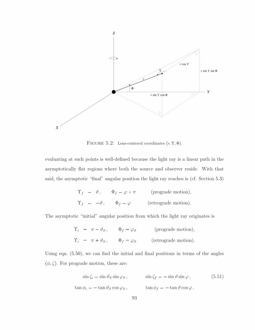
X

Y

Z

æ

æ

r sin U sin F

r cos U

r sin U cos F

r

U

F

ô

ò

ò

Figure 5.2: Lens-centered coordinates pr, Υ, Φq.evaluating at such points is well-defined because the light ray is a linear path in the

asymptotically flat regions where both the source and observer reside. With that

said, the asymptotic “final” angular position the light ray reaches is (cf. Section 5.3)

Υf ϑ , Φf ϕ π (prograde motion),

Υf ϑ , Φf ϕ (retrograde motion).

The asymptotic “initial” angular position from which the light ray originates is

Υi π ϑS , Φf ϕS (prograde motion),

Υi π ϑS , Φf ϕS (retrograde motion).

Using eqn. (5.50), we can find the initial and final positions in terms of the anglespφ, ζq. For prograde motion, these are:

sin ζi sinϑS sinϕS , sin ζf sinϑ sinϕ , (5.51)

tanφi tanϑS cosϕS , tanφf tanϑ cosϕ .

93

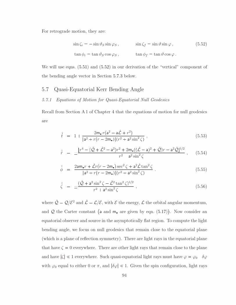
For retrograde motion, they are:

sin ζi sinϑS sinϕS , sin ζf sinϑ sinϕ , (5.52)

tanφi tanϑS cosϕS , tanφf tanϑ cosϕ .

We will use eqns. (5.51) and (5.52) in our derivation of the “vertical” component of

the bending angle vector in Section 5.7.3 below.

5.7 Quasi-Equatorial Kerr Bending Angle

5.7.1 Equations of Motion for Quasi-Equatorial Null Geodesics

Recall from Section A1 of Chapter 4 that the equations of motion for null geodesics

are 9t 1 2m rpa2 aL r2qra2 rpr 2m qspr2 a2 sin2 ζq , (5.53)9r rr4 pQ L2 a2qr2 2m ppL aq2 Qqr a

2Qs12r2 a2 sin2 ζ

, (5.54)9φ 2am r Lrpr 2m q sec2 ζ a2L tan2 ζra2 rpr 2m qspr2 a2 sin2 ζq . (5.55)9ζ pQ a

2 sin2 ζ L2 tan2 ζq12r2 a2 sin2 ζ

, (5.56)

where Q QE2 and L LE , with E the energy, L the orbital angular momentum,

and Q the Carter constanta and m are given by eqn. (5.17)

. Now consider an

equatorial observer and source in the asymptotically flat region. To compute the light

bending angle, we focus on null geodesics that remain close to the equatorial plane

(which is a plane of reflection symmetry). There are light rays in the equatorial plane

that have ζ 0 everywhere. There are other light rays that remain close to the plane

and have |ζ| ! 1 everywhere. Such quasi-equatorial light rays must have ϕ ϕ0δϕwith ϕ0 equal to either 0 or π, and |δϕ| ! 1. Given the spin configuration, light rays

94

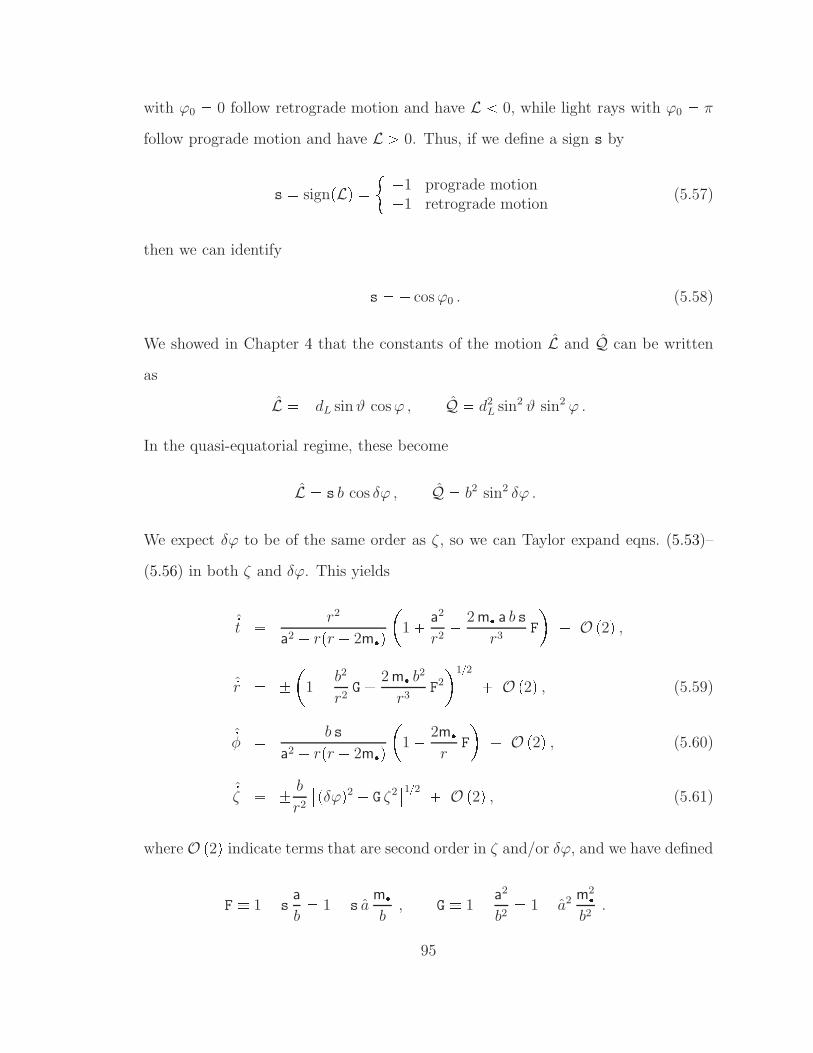
with ϕ0 0 follow retrograde motion and have L 0, while light rays with ϕ0 π

follow prograde motion and have L ¡ 0. Thus, if we define a sign s by

s signpLq " 1 prograde motion1 retrograde motion(5.57)

then we can identify

s cosϕ0 . (5.58)

We showed in Chapter 4 that the constants of the motion L and Q can be written

as

L dL sinϑ cosϕ , Q d2L sin2 ϑ sin2 ϕ .

In the quasi-equatorial regime, these become

L s b cos δϕ , Q b2 sin2 δϕ .

We expect δϕ to be of the same order as ζ , so we can Taylor expand eqns. (5.53)–

(5.56) in both ζ and δϕ. This yields9t r2

a2 rpr 2m q 1 a2

r2 2 m a b s

r3F

O p2q ,9r 1 b2

r2G 2 m b2

r3F2

12 O p2q , (5.59)9φ b s

a2 rpr 2m q 1 2m r

F

O p2q , (5.60)9ζ b

r2

pδϕq2 G ζ212 O p2q , (5.61)

where O p2q indicate terms that are second order in ζ and/or δϕ, and we have defined

F 1 sa

b 1 s a

m b, G 1 a

2

b2 1 a2 m

2 b2

.

95

Notice that 9t, 9r, and 9φ do not depend on ζ or δϕ at zeroth order or first order.

In other words, the “in plane” motion is insensitive to small displacements above

or below the equatorial plane. By contrast, 9ζ lacks a zeroth-order term but has a

nonzero first-order term. Thus, there is a solution with ζ δϕ 0 (i.e., a ray that

stays in the equatorial plane), but there are also solutions in which ζ and δϕ are

nonzero.

Before evaluating the quasi-equatorial light bending, we need to relate the light

ray’s coordinate distance of closest approach, r0, to the invariant impact parameter b.

The distance of closest approach is given by the solution of 9r 0. From eqn. (5.59)

this is a simple quadratic equation in b, whose positive real solution is

b

r0

G 2m r0

F2

12. (5.62)

Alternatively, 9r 0 is a cubic equation in r0, whose one real solution is given by

r0

b 2

312 G12 cos

1

3cos1

332 F2

G32 m b

. (5.63)

Taylor expanding in m b ! 1 yields

r0

b G12 F2

G

m b

3 F4

2 G52 m b

2 4 F6

G4

m b

3 105 F8

8 G112 m b

4 48 F10

G7

m b

5 3003 F12

16 G172 m b

6 O

m b

7

. (5.64)

(We could further expand F and G as Taylor series in m b, but choose not to do that

yet.) Note that in the absence of spin (a 0), F G 1 and so eqns. (5.62)–(5.64)

reduce to their respective Schwarzschild values in Keeton and Petters (2006b).

96

5.7.2 Horizontal Light Bending Angle

We consider the bending of a null geodesic along the φ-direction (horizontal). From

eqns. (5.59) and (5.60), we can write the equation of motion as

dφ

dr 9φ9r s b r12 pr 2 m Fqra2 r pr 2m qsrr3 b2 p2 m F2 G rqs12 . (5.65)

To understand the sign, consider Figs. 4.3 and 4.4. In the case of retrograde motion,

φf ϑ and φi π ϑS, with φi ¡ φf (cf. Section 5.3); recall from Section 5.3

that ϑ and ϑS are the respective projections onto the xy-plane of the angles ϑ and

ϑS. For the “incoming” ray segment (from the source the point of closest approach),

we have (see, e.g., (Weinberg, 1972, p. 189)),

φi φ0 » 8r0

dφdr dr ,where φ0 is the value of φ at the point of closest approach. For the “outgoing”

segment (from the observer the point of closest approach), we have

φ0 φf » 8r0

dφdr dr .Putting them together yields

π ϑS ϑ φi φf 2

» 8r0

dφdr dr .Identifying ϑ ϑS as the “horizontal” bending angle αhor (see eqn. (5.7)), we can

rewrite this equation in the more familiar form (cf. Keeton and Petters (2006b))

αhor 2

» 8r0

dφdr dr π . (5.66)

97

In the case of prograde motion, we have φf ϑ and φi pπ ϑSq with φf ¡ φi.

Similar logic then yields

π ϑS ϑ φf φi 2

» 8r0

dφdr dr . (5.67)

Identifying ϑ ϑS αhor again yields eqn. (5.66).

Thus, eqn. (5.66) represents the general expression for the “horizontal” compo-

nent of the bending angle. The integrand depends on the invariant impact parameter,

b, but the integral itself also depends on the coordinate distance of closest approach,

r0. For pedagogical purposes, and to connect with previous studies of lensing by

Kerr black holes, it is useful to express the integral purely in terms of r0, and later

to convert back to b.

In the weak-deflection regime, r 2m and r 2 m F are always positive, so

all factors in eqn. (5.65) are positive except for s 1. Hence the absolute value

in eqn. (5.66) simply removes the factor of s. Changing integration variables to

x r0r, we can write the bending angle as

αhor 2

» 1

0

1 2 Fh xp1 2 h x a2 h2 x2q rGp1 x2q 2 F2 hp1 x3qs12 dx π ,

where h m r0, and we have used eqn. (5.62) to substitute for b in terms of r0. In

the weak-deflection regime h ! 1, so we can expand the integrand as a Taylor series

in h and then integrate term by term to obtain

αhorphq c0 π 4 c1 h 4 c2 15π

4d2

h2

122

3c3 15π

2d3

h3 130 c4 3465π

64d4

h4 O phq5 , (5.68)

98

where

c0 1

G12 1 ,

c1 F2 G F G

G32 ,

c2 F2pF2 G F GqG52 ,

d2 1

15 G52 15 F4 4 G pF 1q p3 F2 2 Gq 2 a2 G2

,

c3 1

61 G72 61 F6 G pF 1q p45 F4 32 F2 G 16 G2q 4 G2 a2p2 F2 2 G F Gq ,

d3 F2

Gd2 ,

c4 F2

65 G92 65 F6 49pF 1q F4 G 8F2 p4 a2 4 Fq G2 4

4 a2pF 2q 4 F

G3,

d4 1

1155 G92 1155 F8 840pF 1q F6 G 140 F4p4 a2 4 Fq G2 80p4 a2pF 2q 4 Fq F2 G3 8p16 12a2 a4 8pa2 2q Fq G4.

(Terms beyond order four in the bending angle series can be derived but are not

used in our study.) In the absence of spin, we have a 0 and F G 1, so the

coefficients become

c0 0, c1 c2 c3 d2 d3 c4 d4 1.

In this limit, eqn. (5.68) reduces to the Schwarzschild result in Keeton and Petters

(2006b).

Let us briefly consider the bending angle to lowest order in m r0 and ar0. At

first order, b r0 so from eqn. (5.62) we have F 1 s ar0 and G 1. This yields

99

c0 0 and c1 1 s ar0. So to lowest order eqn. (5.68) gives

αhor 4m r0

1 s

a

r0

,

which recovers the known result for such a regime (see., e.g., Boyer and Lindquist

(1967), p. 281).

The expression (5.68) is coordinate-dependent because it involves the coordinate

distance of closest approach, r0. We must rewrite the formula in terms of the impact

parameter b to obtain an invariant result. We use eqn. (5.63) to write h m r0 as

a Taylor series in m b,h 1

G12 m b

F2

G2

m b

2 5 F4

2 G72 m b

3 8 F6

G5

m b

4 231 F8

8 G132 m b

5 112 F10

G8

m b

6 O

m b

7

, (5.69)

and insert this into eqn. (5.68) to obtain a series expansion for the bending angle in

m b:αhorpbq C0 C1

m b

C2

m b

2 C3

m b

3 C4

m b

4 O

m b

5

,

(5.70)

100

where

C0 1

G12 1

π ,

C1 4F2 G F G

G2,

C2 π

4 G72 15 F4 4 G pF 1q p3 F2 2 Gq 2 a2 G2

,

C3 8

3 G5

16F6 4 G pF 1q p3 F4 2 F2 G G2q a2 G2p2 F2 2 G F Gq ,

C4 3π

64 G132 1155 F8 840pF 1qF6 G 140 F4 p4 a2 4 Fq G2 80

4 a2pF 2q 4 F

F2 G3 8

16 12a2 a4 8pa2 2q F G4

.

Eqn. (5.70) holds for values of F and G where the spin is bounded, a2 1. In other

words, when expanding in m b we really ought to expand in ab as well. Formally,

we may accomplish this by writing F and G in terms of a and m b as in eqn. (5.62),

expanding the coefficients Ci as Taylor series in m b, and collecting terms to obtain

a new series expansion for the bending angle. The result is:

αhorpbq A1

m b

A2

m b

2 A3

m b

3 A4

m b

4 O

m b

5

,

where

A1 4 , (5.71)

A2 15π

4 4 s a , (5.72)

A3 128

3 10 π s a 4 a2 , (5.73)

A4 3465π

64 192 s a 285π a2

16 4 s a3 . (5.74)

(Recall that a2 1.) When there is no spin pa 0q, the coefficients reduce to

101

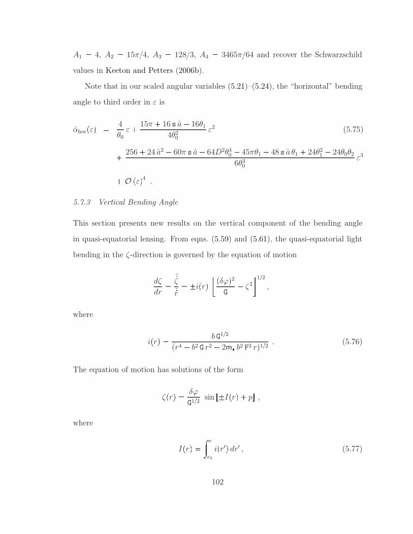
A1 4, A2 15π4, A3 1283, A4 3465π64 and recover the Schwarzschild

values in Keeton and Petters (2006b).

Note that in our scaled angular variables (5.21)–(5.24), the “horizontal” bending

angle to third order in ε is

αhorpεq 4

θ0ε 15π 16 s a 16θ1

4θ20

ε2 (5.75) 256 24 a2 60π s a 64D2θ40 45πθ1 48 s a θ1 24θ2

1 24θ0θ26θ3

0

ε3 O pεq4 .

5.7.3 Vertical Bending Angle

This section presents new results on the vertical component of the bending angle

in quasi-equatorial lensing. From eqns. (5.59) and (5.61), the quasi-equatorial light

bending in the ζ-direction is governed by the equation of motion

dζ

dr 9ζ9r iprq pδϕq2

G ζ2

12,

where

iprq b G12pr4 b2 G r2 2m b2 F2 rq12 . (5.76)

The equation of motion has solutions of the form

ζprq δϕ

G12 sin rIprq ps ,where

Iprq » r

r0

ipr1q dr1 , (5.77)

102

and p is a constant of integration. We are interested in the two asymptotic values

(r Ñ8),

ζ δϕ

G12 sin pI8 pq ,where I8 limrÑ8 Iprq. We can eliminate p and relate the two solutions to one

another:

ζ δϕ

G12 sin

2I8 sin1

G12δϕ

ζ . (5.78)

The asymptotic values ζ must correspond to the initial and final values, ζi and ζf ,

introduced in Section 5.6, but we must determine the correspondence. In order to

do that, we first examine ζi and ζf more carefully, using eqn. (5.51). Recall that

in the quasi-equatorial regime we have ϕ ϕ0 δϕ and ϕS ϕ0 π δϕS, with

ϕ0 π for prograde motion and ϕ0 0 for retrograde motion. Using these relations,

eqns. (5.51) and (5.52) both become

sin ζi sinϑS sin δϕS, sin ζf sinϑ sin δϕ .

Since we are working to first order in ζ and δϕ, we can write these as

ζi δϕS sinϑS , ζf δϕ sin ϑ .

Upon considering the spherical case (see below), we recognize that we want to put

ζ ζi and ζ ζf in eqn. (5.78). This substitution yields

δϕS δϕ

G12 sin ϑS

sin2I8 sin1

G12 sinϑ

W pϑqsinϑS

δϕ . (5.79)

Notice that the coefficient of δϕ depends only on ϑ, not on ϕ. (In addition to

the explicit ϑ dependence, there is implicit dependence through ϑS and I8, which

103

depends on b dL sinϑ.) We can therefore define it to be the function W pϑq, with

a factor of sin ϑS that will prove to be convenient later.

Before evaluating I8, let us check the case of a spherical lens to make sure our

result is reasonable. For a spherical lens, a 0 and F G 1, so we have

2I8 2

» 8r0

b dr

r12rr3 b2pr 2m qs12 π ϑS ϑ ,

where the last equality is obtained after comparison with the spherical limits of

eqns. (5.65) and (5.66). Together with our choices ζ ζi and ζ ζf , eqn. (5.79)

then becomes

δϕS δϕ

sinϑS

sinπ ϑS ϑ sin1psinϑq δϕ ,

which is consistent with the symmetry. This verifies our choice of signs above.

We now evaluate the integral (for the general case, not just the spherical limit),

in parallel with the analysis in Section 5.7.2. From eqns. (5.76) and (5.77) we have

I8 » 8r0

b G12pr4 b2 G r2 2m b2 F2 rq12 dr .Using eqn. (5.62) for b and changing integration variables to x r0r yields

I8 » 1

0

G12rGp1 x2q 2 F2 hp1 x3qs12 dx ,where h m r0. Taylor expanding in h and integrating term by term gives

I8 π

2 2 F2

Gh F4

8 G2p15π 16q h2 F6

12 G3p244 45πq h3 5F8

128 G4p1664 693πq h4 O phq5 .

104

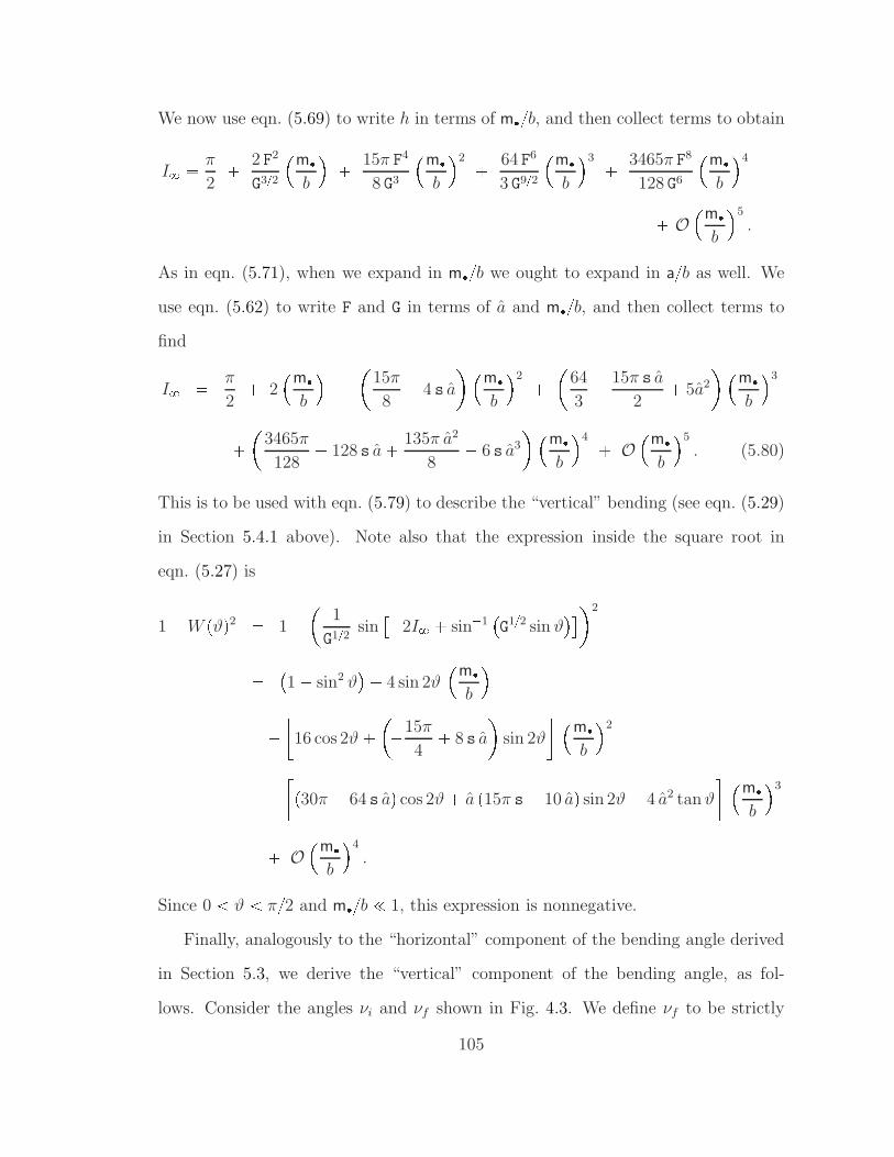
We now use eqn. (5.69) to write h in terms of m b, and then collect terms to obtain

I8 π

2 2 F2

G32 m b

15π F4

8 G3

m b

2 64 F6

3 G92 m b

3 3465π F8

128 G6

m b

4 O

m b

5

.

As in eqn. (5.71), when we expand in m b we ought to expand in ab as well. We

use eqn. (5.62) to write F and G in terms of a and m b, and then collect terms to

find

I8 π

2 2

m b

15π

8 4 s a

m b

2 64

3 15π s a

2 5a2

m b

3 3465π

128 128 s a 135π a2

8 6 s a3

m b

4 O

m b

5

. (5.80)

This is to be used with eqn. (5.79) to describe the “vertical” bending (see eqn. (5.29)

in Section 5.4.1 above). Note also that the expression inside the square root in

eqn. (5.27) is

1W pϑq2 1 1

G12 sin2I8 sin1

G12 sin ϑ

2 1 sin2 ϑ

4 sin 2ϑ

m b

16 cos 2ϑ 15π

4 8 s a

sin 2ϑ

m b

2 p30π 64 s aq cos 2ϑ a p15π s 10 aq sin 2ϑ 4 a2 tanϑ

m b

3 O

m b

4

.

Since 0 ϑ π2 and m b ! 1, this expression is nonnegative.

Finally, analogously to the “horizontal” component of the bending angle derived

in Section 5.3, we derive the “vertical” component of the bending angle, as fol-

lows. Consider the angles νi and νf shown in Fig. 4.3. We define νf to be strictly

105

nonnegative and within the interval r0, π2q, but allow νi to be negative, so thatπ2 νi π2, and enforce the following sign convention for νi. As shown in

Fig. 4.3, νi is the angle whose vertex is the point B1 on the lens plane, and is mea-

sured from a line parallel to the equatorial plane. If νi goes away from the equatorial

plane, then we take it to be positive; otherwise it is negative (e.g., the νi shown in

Fig. 4.3 is positive). Now denote by νi and νf the respective projections onto the

xz-plane of the angles νi and νf , and adopt the same sign conventions for them.

With these conventions, the “vertical” component of the bending angle can be un-

ambiguously expressed as

αvert νf νi .

By the positivity of νf and the fact that the bending is nonnegative, we have

νi ¤ νf .

(Indeed, with our signs conventions the condition νi ¡ νf would be equivalent to

repulsion of the light ray.) Writing νi and νf in terms of the angles ϑ, ϕ, ϑS, ϕS, we

have

νf tan1ptanϑ sinϕq ,νi tan1ptanϑS sinpπ ϕSqq ,

which in the quasi-equatorial regime reduce to

νf δϕ tanϑ ,

νi δϕS tanϑS ,

where we have set ϕ ϕ0 δϕ, δϕS ϕ0 π δϕS, with ϕ0 0 (retrograde

motion) or π (prograde motion), and expanded to linear order in the small angles

δϕ and δϕS. Using the identities W pϑq δϕ sinϑS δϕS and ϑS αhor ϑ given by

106

eqns. (5.79) and (5.11), we can thus write αvert as

αvert δϕ tanϑ W pϑqcospαhor ϑq .

The expression inside the square brackets is of the form 16D csc ϑ sec2 ϑ ε2O pεq4,so it is positive (recall that 0 ϑ π2). Since the bending angle is strictly

nonnegative, we will adopt “ ” for δϕ ¥ 0 and “ ” for δϕ 0, so that we may

write

αvert δϕ

tanϑ W pϑq

cospαhor ϑq . (5.81)

We now expand eqn. (5.81) in our scaled angular variables (5.21)–(5.24) to third

order in ε to obtain

αvertpεq δϕ

#tanϑ 1

G12 sin2I8 sin1

G12 sin ϑ

1

cospαhor ϑq+ δϕ

#4

θ0ε 15π 32 s a 16θ1

4θ20

ε2 256 72 a2 90π s a 64D2θ40 96 s a θ1 45πθ1 24θ2

1 24θ0θ26θ3

0

ε3O pεq4+ . (5.82)

The result in eqn. (5.82) is new.

5.8 Quasi-Equatorial Time Delay

We now compute the time delays for quasi-equatorial lensed images. Let Rsrc and

Robs be the radial coordinates of the source and observer, respectively. From geom-

etry relative to the flat metric of the distant observer, who is assumed to be at rest

107

in the Boyer-Lindquist coordinates, we can work out

Robs dL , Rsrc d2

LS d2S tan2 B

12.

The radial distances are very nearly the same as angular diameter distances since

the source and observer are in the asymptotically flat region of the spacetime. In the

absence of the lens, the spacetime would be flat and the light ray would travel along

a linear path of length dS cosB from the source to the observer.

The time delay is the difference between the light travel time for the actual ray,

and the travel time for the ray the light would have taken had the lens been absent.

This can be written as

cτ T pRsrcq T pRobsq dS

cosB,

with

T pRq » R

r0

dtdr dr » R

r0

9t9r dr .We use 9t and 9r from eqns. (5.59) and (5.59), substitute for b using eqn. (5.62), and

change integration variables to x r0r. This yields

T pRq r0

» 1

r0R pG 2 F2 hq12p1 a2 h2 x2q 2 s a Fh2 x3

x2 p1 2 h x a2 h2 x2q rGp1 x2q 2 F2 hp1 x3qs12 dx ,where h m r0. We expand the integrand as a Taylor series in h and integrate

term by term. The result is a series in h whose coefficients are rational functions of

108

ω r0R. The first three terms in the expansion are

T pRq bR2 r2

0 h r0

F2?

1 ω2

Gp1 ωq 2 ln

1?1 ω2

ω

(5.83) h2 r0

3 F4 4 F2 G 8 G2

2 G2

π2 sin1 ω

2 s a F G12?1 ω2 F2 p4 G pF2 4 Gqωq?1 ω2

2 G2 p1 ωq2 O phq3 .

The third-order term is easily obtained, and is needed in the derivation of eqn. (5.48),

but is too unweildy to write here. Note that if we substitute for F and G using

eqn. (5.62) and take the far-field limit, we recover previous results (e.g., Dymnikova

(1984, 1986)).

109

6

Future Goals

One of my future explorations is a systematic study of magnification relations in the

Kerr black hole geometry in the non-quasi-equatorial case.

110

Bibliography

Aazami, A. and Petters, A. (2009a), “A universal magnification theorem for higher-order caustic singularities,” Journal of Mathematical Physics, 50, 032501.

Aazami, A. and Petters, A. (2009b), “A universal magnification theorem. II. Genericcaustics up to codimension five,” Journal of Mathematical Physics, 50, 082501.

Aazami, A. and Petters, A. (2010), “A universal magnification theorem. III. Causticsbeyond codimension 5,” Journal of Mathematical Physics, 51, 023503.

Aazami, A., Keeton, C., and Petters, A. (2011a), “Lensing by Kerr black holes.II: Analytical study of quasi-equatorial lensing observables,” Arxiv preprintarXiv:1102.4304.

Aazami, A., Petters, A., and Rabin, J. (2011b), “Orbifolds, the A,D,E family ofcaustic singularities, and gravitational lensing,” Journal of Mathematical Physics,52, 022501.

Adem, A., Leida, J., and Ruan, Y. (2007), Orbifolds and Stringy Topology, Cam-bridge University Press.

Arnold, V. (1973), “Normal forms for functions near degenerate critical points, theWeyl groups of Ak, Dk, Ek and Lagrangian singularities,” Functional Analysis andIts Applications, 6, 254–272.

Arnold, V., Gusein-Zade, S., and Varchenko, A. (1985), “Singularities of Differen-tiable Maps, Volume I,” Birkhauser, Boston.

Barbeau, E. (2003), Polynomials, Springer.

Blandford, R. and Narayan, R. (1986), “Fermat’s principle, caustics, and the classi-fication of gravitational lens images,” The Astrophysical Journal, 310, 568–582.

Boyer, R. and Lindquist, R. (1967), “Maximal analytic extension of the Kerr metric,”Journal of Mathematical Physics, 8, 265.

Bozza, V. (2003), “Quasiequatorial gravitational lensing by spinning black holes inthe strong field limit,” Physical Review D, 67, 103006.

111

Bozza, V. (2008a), “Comparison of approximate gravitational lens equations and aproposal for an improved new one,” Physical Review D, 78, 103005.

Bozza, V. (2008b), “Optical caustics of Kerr spacetime: The full structure,” PhysicalReview D, 78, 63014.

Bozza, V. and Scarpetta, G. (2007), “Strong deflection limit of black hole gravita-tional lensing with arbitrary source distances,” Physical Review D, 76, 83008.

Bozza, V. and Sereno, M. (2006), “Weakly perturbed Schwarzschild lens in the strongdeflection limit,” Physical Review D, 73, 103004.

Bozza, V., De Luca, F., Scarpetta, G., and Sereno, M. (2005), “Analytic Kerr blackhole lensing for equatorial observers in the strong deflection limit,” Physical ReviewD, 72, 83003.

Bozza, V., Luca, F., and Scarpetta, G. (2006), “Kerr black hole lensing for genericobservers in the strong deflection limit,” Physical Review D, 74, 63001.

Carter, B. (1968), “Global structure of the Kerr family of gravitational fields,” Phys-ical Review, 174, 1559–1571.

Castrigiano, D. and Hayes, S. (2004), Catastrophe Theory, Westview Press.

Cattani, E., Dickenstein, A., and Sturmfels, B. (1997a), “Residues and resultants,”Arxiv preprint alg-geom/9702001.

Cattani, E., Cox, D., and Dickenstein, A. (1997b), “Residues in toric varieties,”Compositio Mathematica, 108, 35–76.

Chiba, M. (2002), “Probing dark matter substructure in lens galaxies,” The Astro-physical Journal, 565, 17.

Congdon, A. and Keeton, C. (2005), “Multipole models of four-image gravitationallenses with anomalous flux ratios,” Monthly Notices of the Royal AstronomicalSociety, 364, 1459–1466.

Dalal, N. (1998), “The magnification invariant of simple galaxy lens models,” TheAstrophysical Journal Letters, 509, L13.

Dalal, N. and Rabin, J. (2001), “Magnification relations in gravitational lensing viamultidimensional residue integrals,” Journal of Mathematical Physics, 42, 1818.

Dymnikova, I. (1984), “The effect of the relative delay of rays focused by a rotatingmassive body,” Zhurnal Eksperimental noi i Teoreticheskoi Fiziki, 86, 385–389.

Dymnikova, I. (1986), “Motion of particles and photons in the gravitational field ofa rotating body.” Uspekhi Fizicheskikh Nauk, 148, 393–432.

112

Evans, N. and Witt, H. (2003), “Fitting gravitational lenses: truth or delusion,”Monthly Notices of the Royal Astronomical Society, 345, 1351–1364.

Golubitsky, M. and Guillemin, V. (1973), Stable Mappings and Their Singularities,Springer Verlag.

Griffiths, P. and Harris, J. (1978), Principles of Algebraic Geometry, vol. 1994, WileyNew York.

Hunter, C. and Evans, N. (2001), “Lensing properties of scale-free galaxies,” TheAstrophysical Journal, 554, 1227.

Iyer, S. and Hansen, E. (2009a), “Light’s bending angle in the equatorial plane of aKerr black hole,” Physical Review D, 80, 124023.

Iyer, S. and Hansen, E. (2009b), “Strong and Weak Deflection of Light in the Equa-torial Plane of a Kerr Black Hole,” Arxiv preprint arXiv:0908.0085.

Keeton, C. (2001), “Computational methods for gravitational lensing,” Arxivpreprint astro-ph/0102340.

Keeton, C. and Petters, A. (2005), “Formalism for testing theories of gravity usinglensing by compact objects: Static, spherically symmetric case,” Physical ReviewD, 72, 104006.

Keeton, C. and Petters, A. (2006a), “Formalism for testing theories of gravity usinglensing by compact objects. II. Probing post-post-Newtonian metrics,” PhysicalReview D, 73, 44024.

Keeton, C. and Petters, A. (2006b), “Formalism for testing theories of gravity us-ing lensing by compact objects. III. Braneworld gravity,” Physical Review D, 73,104032.

Keeton, C., Gaudi, B., and Petters, A. (2003), “Identifying lenses with small-scalestructure. I. Cusp lenses,” The Astrophysical Journal, 598, 138.

Keeton, C., Gaudi, B., and Petters, A. (2005), “Identifying lenses with small-scalestructure. II. Fold lenses,” Astrophysical Journal, 635, 35–59.

Lee, J. (2003), Introduction to Smooth Manifolds, Springer Verlag.

Majthay, A. (1985), Foundations of Catastrophe Theory, Pitman Advanced Pub.Program.

Mao, S. and Schneider, P. (1997), “Evidence for substructure in lens galaxies?” Arxivpreprint astro-ph/9707187.

113

Metcalf, R. and Madau, P. (2001), “Compound gravitational lensing as a probe ofdark matter substructure within galaxy halos,” The Astrophysical Journal, 563, 9.

Moerdijk, I. and Pronk, D. (1997), “Orbifolds, sheaves and groupoids,” K-theory, 12,3–21.

O’Neill, B. (1995), The Geometry of Kerr Black Holes, AK Peters, AK Peters.

Petters, A. (2010), “Gravity’s Action on Light,” Notices of the AMS, 57.

Petters, A., Levine, H., and Wambsganss, J. (2001), Singularity Theory and Gravi-tational Lensing, Birkhauser.

Rauch, K. and Blandford, R. (1994), “Optical caustics in a kerr spacetime andthe origin of rapid x-ray variability in active galactic nuclei,” The AstrophysicalJournal, 421, 46–68.

Rhie, S. (1997), “Infimum microlensing amplification of the maximum number ofimages of n-point lens systems,” The Astrophysical Journal, 484, 63.

Satake, I. (1956), “On a generalization of the notion of manifold,” Proceedings of theNational Academy of Sciences of the United States of America, 42, 359.

Schneider, P. and Weiss, A. (1992), “The gravitational lens equation near cusps,”Astronomy and Astrophysics, 260, 1–13.

Schneider, P., Ehlers, J., and Falco, E. (1992), Gravitational Lenses, Springer Verlag.

Sereno, M. and De Luca, F. (2006), “Analytical Kerr black hole lensing in the weakdeflection limit,” Physical Review D, 74, 123009.

Sereno, M. and De Luca, F. (2008), “Primary caustics and critical points behind aKerr black hole,” Physical Review D, 78, 23008.

Vazquez, S. and Esteban, E. (2003), “Strong field gravitational lensing by a Kerrblack hole,” NUOVO CIMENTO-SOCIETA ITALIANA DI FISICA SEZIONEB, 119, 489.

Virbhadra, K. and Ellis, G. (2000), “Schwarzschild black hole lensing,” PhysicalReview D, 62, 84003.

Virbhadra, K. and Ellis, G. (2002), “Gravitational lensing by naked singularities,”Physical Review D, 65, 103004.

Wald, R. (1984), General Relativity, University of Chicago Press.

Weinberg, S. (1972), Gravitation and Cosmology, vol. 7, Wiley New York.

114

Werner, M. (2007), “A Lefschetz fixed point theorem in gravitational lensing,” Jour-nal of Mathematical Physics, 48, 052501.

Werner, M. (2009), “Geometry of universal magnification invariants,” Journal ofMathematical Physics, 50, 082504.

Werner, M. and Petters, A. (2007), “Magnification relations for Kerr lensing andtesting cosmic censorship,” Physical Review D, 76, 64024.

Witt, H. and Mao, S. (1995), “On the minimum magnification between caustic cross-ings for microlensing by binary and multiple stars,” The Astrophysical JournalLetters, 447, L105.

Witt, H. and Mao, S. (2000), “On the magnification relations in quadruple lenses:a moment approach,” Monthly Notices of the Royal Astronomical Society, 311,689–697.

Zakharov, A. (1995), “On the magnification of gravitational lens images near cusps.”Astronomy and Astrophysics, 293, 1–4.

115

Biography

Amir Babak Aazami was born December 14, 1978, in Tehran, Iran. Together with

his family, he immigrated to the United States in 1985. He attended the University

of California, Berkeley, graduating in 2001 with a Bachelor’s in Physics and English

literature. He has since focused on mathematical physics. He hopes to carry on

doing research in academia.

116