public transport model development report
TRANSCRIPT
Modelling Services Framework
East Regional Model
Public Transport Model Development Report
ERM Public Transport Model Development Report | 1
CONTENTS
Foreword ............................................................................................ 5
1 Introduction.................................................................................. 6
1.1 Regional Modelling System ........................................................................... 6
1.2 Regional Modelling System Structure ........................................................... 8
1.3 ERM Public Transport Model Overview ...................................................... 11
1.4 This Report .................................................................................................. 14
2 ERM PT Model Development .................................................... 16
2.1 Overview ..................................................................................................... 16
2.2 Public Transport Services Preparation ........................................................ 21
2.3 Fares Model Preparation ............................................................................. 24
2.4 Wait Curve Preparation ............................................................................... 33
2.5 Crowding Model Preparation ....................................................................... 34
3 ERM Cube Voyager Implementation ........................................ 36
3.1 Overview ..................................................................................................... 36
3.2 Inputs .......................................................................................................... 36
3.3 Network Link Attributes ............................................................................... 38
3.4 Key Parameters .......................................................................................... 39
3.5 Outputs........................................................................................................ 40
4 PT Model Calibration ................................................................. 43
4.1 Introduction ................................................................................................. 43
4.2 Assignment Calibration Process ................................................................. 43
4.3 PT Model Network Progression ................................................................... 44
4.4 PT Model Parameters Progression ............................................................. 49
4.5 PT Model Matrix Progression ...................................................................... 57
4.6 Summary ..................................................................................................... 72
5 PT Model Validation................................................................... 73
5.1 Introduction ................................................................................................. 73
5.2 Assignment Validation Process ................................................................... 73
5.3 Observed data ............................................................................................. 74
5.4 PT Trip Matrix Validation ............................................................................. 76
5.5 PT Network Validation ................................................................................. 78
5.6 PT Assignment Validation - Boarding and Alighting .................................... 82
5.7 PT Assignment Validation - Line profiles ..................................................... 85
5.8 Interchange ................................................................................................. 89
6 Conclusion and Recommendations ......................................... 91
6.1 Summary ..................................................................................................... 91
6.2 Model Development – Key points ................................................................ 91

ERM Public Transport Model Development Report | 2
6.3 Model Validation .......................................................................................... 91
6.4 Recommendations ...................................................................................... 92
TABLES Table 1.1 Regional Models and their Population Centres ...................................... 6
Table 1.2 ERM Time Periods ............................................................................... 14
Table 2.1 Irish Rail Fares Models ........................................................................ 26
Table 2.2 Modelled vs Observed Average Fares ................................................. 29
Table 2.3 Wait Curve Definition ........................................................................... 33
Table 3.1 Additional PTM Network Files .............................................................. 37
Table 3.2 PT Model Parameters .......................................................................... 40
Table 3.3 PT Model Outputs ................................................................................ 41
Table 4.1 Summary of Generalised Cost Tests carried out in SWRM ................. 46
Table 4.2 Detailed Network Audit Recommendations .......................................... 48
Table 4.3 Summary of Parameter Options Retained for Revised PTAM ............. 51
Table 4.4 Wait Curve Definition ........................................................................... 53
Table 4.5 Detailed Parameter Audit Recommendations ...................................... 54
Table 4.6 In-vehicle time factors – initial and calibrated values ........................... 54
Table 4.7 Interchange penalties ........................................................................... 55
Table 4.8 Bus speed factors by link characteristics and by time period ............... 56
Table 4.9 Time factors by bus service characteristics and by time period ........... 56
Table 4.10 Significance of Matrix Estimation Changes .......................................... 68
Table 4.11 AM Matrix Change R2 Analysis – Matrix Zonal Cell Values ................. 68
Table 4.12 AM Matrix Change R2 Analysis – Matrix Zonal Trip Ends .................... 69
Table 4.13 LT Matrix Change R2 Analysis – Matrix Zonal Cell Values .................. 69
Table 4.14 LT Matrix Change R2 Analysis – Matrix Zonal Trip Ends ..................... 70
Table 4.15 SR Matrix Change R2 Analysis – Matrix Zonal Cell Values ................. 70
Table 4.16 SR Matrix Change R2 Analysis – Matrix Zonal Trip Ends .................... 71
Table 4.17 PM Matrix Change R2 Analysis – Matrix Zonal Cell Values ................. 71
Table 4.18 PM Matrix Change R2 Analysis – Matrix Zonal Trip Ends .................... 72
Table 5.1 PT Assignment Model Trip Matrix Validation Criteria ........................... 73
Table 5.2 PT Assignment Validation Criteria ....................................................... 74
Table 5.3 CERTU Guide 2003 – Transfer ratio range .......................................... 74
Table 5.4 Bus observed flows data sources ........................................................ 75
Table 5.5 Passenger flow validation summary table ............................................ 77
Table 5.6 Service classification by journey time comparison to AVL data and by
time period ...................................................................................................... 79
Table 5.7 Journey Time validation against AVL data – Summary table ............... 80
Table 5.8 Service classification by journey time comparison to GTFS data and by
time period ...................................................................................................... 81
Table 5.9 Journey Time validation against GTFS data – Summary table ............ 81
Table 5.10 Boarding and alighting validation by mode – AM time period............... 83
Table 5.11 Boarding and alighting validation by mode – LT time period ................ 84

ERM Public Transport Model Development Report | 3
Table 5.12 Boarding and alighting validation by mode – SR time period ............... 84
Table 5.13 Boarding and alighting validation by mode – PM time period............... 85
Table 5.14 Overall PT transfer ratio by time period................................................ 90
ERM Public Transport Model Development Report | 4
FIGURES Figure 1.1 Regional Model Areas............................................................................. 7
Figure 1.2 RMS Model Structure............................................................................ 10
Figure 1.3 ERM Zone System ................................................................................ 13
Figure 2.1 ERM CUBE Voyager PT Road Network ............................................... 17
Figure 2.2: ERM Rail network ................................................................................ 18
Figure 2.3: ERM additional walk links .................................................................... 19
Figure 2.4: ERM PTM PT Lines Files ..................................................................... 24
Figure 2.5: DART Fare model ................................................................................ 27
Figure 2.6: Rosslare-Dundalk line Fare model ....................................................... 27
Figure 2.7: Sligo Line Fare model .......................................................................... 28
Figure 2.8: Southwest line Fare model .................................................................. 28
Figure 2.9: Luas fare system stages ...................................................................... 30
Figure 2.10 Bus Eireann Fare Model ..................................................................... 31
Figure 2.11 Private operators fare models (Airport and non-Airport services) ....... 32
Figure 2.12 Private operators fare models (Airport and non-Airport services) ....... 32
Figure 2.13 Wait Curves ........................................................................................ 34
Figure 2.14 Crowding Curves – Utilisation to Crowding Factors ............................ 35
Figure 3.1 General PT Model Flow ........................................................................ 36
Figure 4.1 Non-Transit Leg PT Access Testing ..................................................... 45
Figure 4.2 Modelled wait curve .............................................................................. 53
Figure 4.3 Canal Cordon PT Count Locations ....................................................... 59
Figure 4.4 Outer Cordon PT Count Locations ........................................................ 60
Figure 4.5 Canal Cordon Screenlines .................................................................... 61
Figure 4.6 ERM Sector System.............................................................................. 61
Figure 4.7 Canal cordon PT screen lines ............................................................... 62
Figure 4.8 Matrix calibration process – Cordon flows - AM peak hour ................... 64
Figure 4.9 Matrix calibration process – Cordon flows - PM peak hour ................... 65
Figure 4.10 24 hour PT matrix sector changes with factoring ................................ 66
Figure 4.11 24 hour PT matrix sector % changes with factoring ............................ 67
Figure 5.1 AVL data routes used in Journey Time validation ................................. 78
Figure 5.2 Bus times scatter plot – AVL Data ........................................................ 80
Figure 5.3 Bus times scatter plot – GTFS Data ..................................................... 82
Figure 5.4 Luas Green line profile – Northbound – AM peak ................................. 86
Figure 5.5 Luas Red line profile – Eastbound – AM peak ...................................... 87
Figure 5.6 DART line profile – Northbound – AM peak .......................................... 88
Figure 5.7 DART line profile – Southbound – AM peak ......................................... 89

ERM Public Transport Model Development Report | 5
Foreword The NTA has developed a Regional Modelling System (RMS) for Ireland that
allows for the appraisal of a wide range of potential future transport and land use
alternatives. The RMS was developed as part of the Modelling Services
Framework (MSF) by the National Transport Authority (NTA), SYSTRA and Jacobs
Engineering Ireland.
The National Transport Authority’s (NTA) Regional Modelling System comprises
the National Demand Forecasting Model, five large-scale, technically complex,
detailed and multi-modal regional transport models and a suite of Appraisal
Modules covering the entire national transport network of Ireland. The five regional
models are focussed on the travel-to-work areas of the major population centres in
Ireland, i.e. Dublin, Cork, Galway, Limerick, and Waterford.
The development of the RMS followed a detailed scoping phase informed by NTA
and wider stakeholder requirements. The rigorous consultation phase ensured a
comprehensive understanding of available data sources and international best
practice in regional transport model development.
The five discrete models within the RMS have been developed using a common
framework, tied together with the National Demand Forecasting Model. This
approach used repeatable methods; ensuring substantial efficiency gains; and, for
the first time, delivering consistent model outputs across the five regions.
The RMS captures all day travel demand, thus enabling more accurate modelling
of mode choice behaviour and increasingly complex travel patterns, especially in
urban areas where traditional nine-to-five working is decreasing. Best practice,
innovative approaches were applied to the RMS demand modelling modules
including car ownership; parking constraint; demand pricing; and mode and
destination choice. The RMS is therefore significantly more responsive to future
changes in demographics, economic activity and planning interventions than
traditional models.
The models are designed to be used in the assessment of transport policies and
schemes that have a local, regional and national impact and they facilitate the
assessment of proposed transport schemes at both macro and micro level and are
a pre-requisite to creating effective transport strategies.
ERM Public Transport Model Development Report | 6
1 Introduction
1.1 Regional Modelling System The NTA has developed a Regional Modelling System for the Republic of Ireland to
assist in the appraisal of a wide range of potential future transport and land use
options. The Regional Models (RM) are focused on the travel-to-work areas of the
major population centres of Dublin, Cork, Galway, Limerick, and Waterford. The
models were developed as part of the Modelling Services Framework by NTA,
SYSTRA and Jacobs Engineering Ireland.
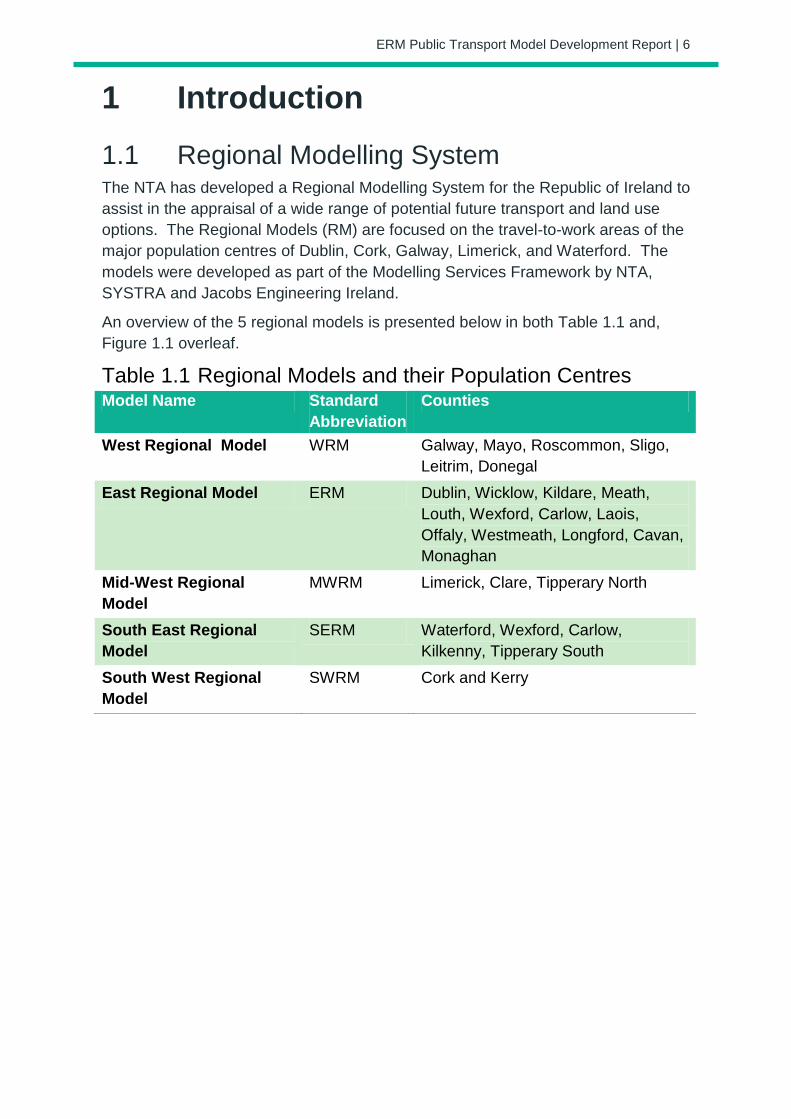
An overview of the 5 regional models is presented below in both Table 1.1 and,
Figure 1.1 overleaf.
Table 1.1 Regional Models and their Population Centres Model Name Standard
Abbreviation
Counties
West Regional Model WRM Galway, Mayo, Roscommon, Sligo,
Leitrim, Donegal
East Regional Model ERM Dublin, Wicklow, Kildare, Meath,
Louth, Wexford, Carlow, Laois,
Offaly, Westmeath, Longford, Cavan,
Monaghan
Mid-West Regional
Model
MWRM Limerick, Clare, Tipperary North
South East Regional
Model
SERM Waterford, Wexford, Carlow,
Kilkenny, Tipperary South
South West Regional
Model
SWRM Cork and Kerry

ERM Public Transport Model Development Report | 7
Figure 1.1 Regional Model Areas

ERM Public Transport Model Development Report | 8
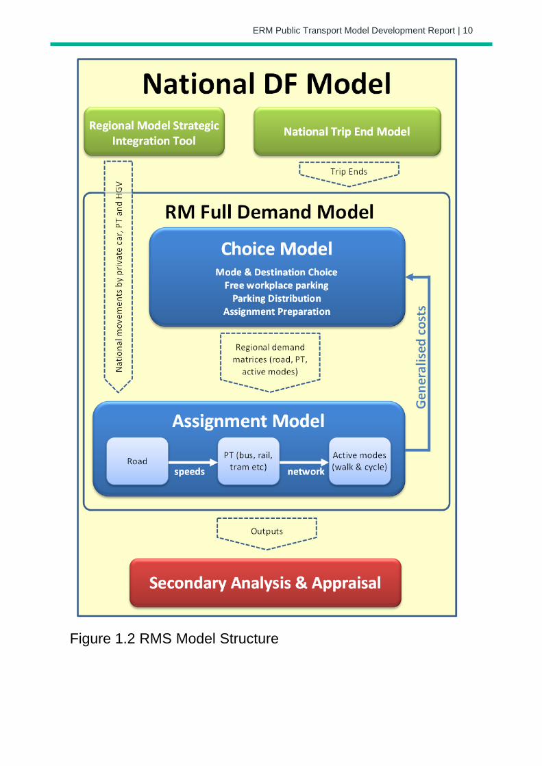
1.2 Regional Modelling System Structure The Regional Modelling System is comprised of three main components, namely:
The National Demand Forecasting Model (NDFM);
5 Regional Models; and
A suite of Appraisal Modules.
The modelling approach is consistent across each of the regional models. The
general structure of the ERM (and the other regional models) is shown below in
Figure 1.2. The main stages of the regional modelling system are described below.
1.2.1 National Demand Forecasting Model (NDFM). The NDFM is a single, national system that provides estimates of the total quantity
of daily travel demand produced by and attracted to each of the 18,488 Census
Small Areas. Trip generations and attractions are related to zonal attributes such
as population, number of employees and other land-use data. See the NDFM
Development Report for further information.
1.2.2 Regional Models (RM) A regional model is comprised of the following key elements:
Trip End Integration The Trip End Integration module converts the 24 hour trip ends output by the
NDFM into the appropriate zone system and time period disaggregation for use in
the Full Demand Model (FDM).
The Full Demand Model (FDM) The FDM processes travel demand and outputs origin-destination travel matrices
by mode and time period to the assignment models. The FDM and assignment
models run iteratively until an equilibrium between travel demand and the cost of
travel is achieved.
See the RM Spec 1 Full Demand Model Specification Report, RM Full Demand
Model Development Report and ERM Full Demand Model Calibration Report for
further information.
Assignment Models The Road, Public Transport, and Active Modes assignment models receive the trip
matrices produced by the FDM and assign them in their respective transport
networks to determine route choice and the generalised cost for origin and
destination pair.
The Road Model assigns FDM outputs (passenger cars) to the road network and
includes capacity constraint, traffic signal delay and the impact of congestion. See
the RM Spec 2 Road Model Specification Report for further information.
The Public Transport Model assigns FDM outputs (person trips) to the PT network
and includes the impact of capacity restraint, such as crowding on PT vehicles, on
people’s perceived cost of travel. The model includes public transport networks

ERM Public Transport Model Development Report | 9
and services for all PT sub-modes that operate within the modelled area. See the
RM Spec 3 Public Transport Model Specification Report for further information
(referred to as the PTM Specification Report for the remainder of this document).
Secondary Analysis The secondary analysis application can be used to extract and summarise model
results from each of the regional models.
1.2.3 Appraisal Modules The Appraisal Modules can be used on any of the regional models to assess the
impacts of transport plans and schemes. The following impacts can be informed
by model outputs (travel costs, demands and flows):
Economy;
Safety;
Environmental;
Health; and
Accessibility and Social Inclusion.
Further information on each of the Appraisal Modules can be found in the following
reports:
Economic Module Development Report;
Safety Module Development Report;
Environmental Module Development Report;
Health Module Development Report; and
Accessibility and Social Inclusion Module Development Report.
ERM Public Transport Model Development Report | 10
Figure 1.2 RMS Model Structure

ERM Public Transport Model Development Report | 11
1.3 ERM Public Transport Model Overview
1.3.1 ERM Public Transport Model Development Public Transport Model development and calibration is a task common to each of
the NTA regional transport models. The PTM Specification Report, that provides a
basis for consistency across all of the models, was used as a guide for the
development of the ERM Public Transport Model.
The development of the ERM has been broken down into a number of high-level
tasks, of which the principal ones are shown below:
Road model development and calibration;
Public transport model development and calibration; and
Demand model development and calibration.
The ERM Public Transport development provides the methodology, guidance and
techniques to develop the Regional Modelling System through a ‘Repeatable
Methods’ approach. The development of Eastern Regional Model Public Transport
Model was based on the specification outlined in PTM Specification Report.
1.3.2 PTM Demand Segmentation The following user classes are defined in the PT assignment model:
Employers-Business (EMP): trips on employers business;
Commute (COM): commuting trips between home and work;
Other (OTH): all other journey purposes including shopping, visiting
friends, escort to education etc;
Non-Dedicated School (SCH): primary and secondary school pupil
trips on general PT services between home and place of education;
Concessionary Travel : passengers eligible for free travel passes on
PT through the Free Travel Scheme; and
Further details are provided in Section 3.8.2 of the PTM Specification Report.
1.3.3 Network Development The ERM PT network comprises a number of input components, as follows:
Road network links (copied directly from SATURN to Cube Voyager
network format);
Walking links (added to the road network to permit walk only paths and
access to rail stations);
Rail links; and
Zone connectors (the connection points from zone centroids to the
‘physical’ network).
ERM Public Transport Model Development Report | 12
1.3.4 Linkages with Overall ERM Transport Model The development of the Regional Model includes a number of inter-dependencies
with other elements of the ERM. These linkages are discussed in later sections
where relevant and can be summarised as follows.
Definition of Zone System
Definition of zonal boundaries for ERM.
System Architecture
Consideration of model procedures and their impact on run-times;
Coordination with overall Regional Modelling System (RMS);
Standardisation with overall RMS (e.g. scripts, procedures, units);
and,
Derivation and calculation of annualisation factors.
In addition, there are a number of inter-dependencies with other elements of ERM:
Road Model
Interchange of key data, notably network details and bus speeds.
Demand Model
Inputs to PT Model
PT Assignment Matrices; and
Generalised Cost parameters and specifically the value of time of
public transport users.
Outputs from PT Model
Cost skims for feedback into mode and destination choice (MDC)
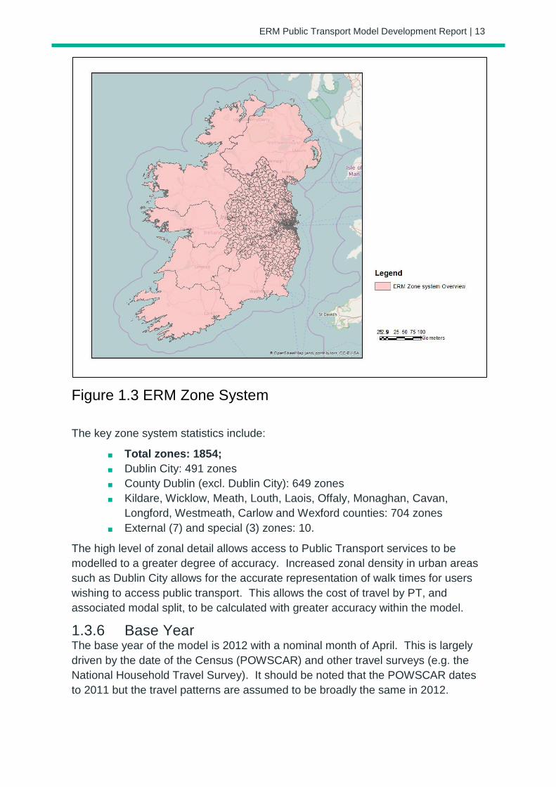
1.3.5 ERM Zone System The PT Model zone system is the same as the zoning system specified for the
overall ERM as described in the ERM Zone System Development Report. The
zone system has 1854 zones and is shown in Figure 1.3 below.
ERM Public Transport Model Development Report | 13
Figure 1.3 ERM Zone System
The key zone system statistics include:
Total zones: 1854;
Dublin City: 491 zones
County Dublin (excl. Dublin City): 649 zones
Kildare, Wicklow, Meath, Louth, Laois, Offaly, Monaghan, Cavan,
Longford, Westmeath, Carlow and Wexford counties: 704 zones
External (7) and special (3) zones: 10.
The high level of zonal detail allows access to Public Transport services to be
modelled to a greater degree of accuracy. Increased zonal density in urban areas
such as Dublin City allows for the accurate representation of walk times for users
wishing to access public transport. This allows the cost of travel by PT, and
associated modal split, to be calculated with greater accuracy within the model.
1.3.6 Base Year The base year of the model is 2012 with a nominal month of April. This is largely
driven by the date of the Census (POWSCAR) and other travel surveys (e.g. the
National Household Travel Survey). It should be noted that the POWSCAR dates
to 2011 but the travel patterns are assumed to be broadly the same in 2012.

ERM Public Transport Model Development Report | 14
1.3.7 Time Periods The five weekday periods modelled in the ERM are detailed in Table 1.2. The time
periods allow the relative differential in travel cost to be represented. The PT
assignment model requires a single hour to be assigned as representative of each
period. Peak hour matrices were obtained from the period matrices by applying
peak hour factors which were calculated from the NHTS based on the mid-point of
the journey time, but without regard to journey purpose.
Table 1.2 ERM Time Periods PERIOD DEMAND
MODEL FULL
PERIOD
ASSIGNMENT
PERIOD
PERIOD TO
PEAK HOUR
FACTORS
AM Peak 07:00-10:00 Peak hour (factored
from period)
0.47
Morning Interpeak
“Lunch Time” (LT)
10:00-13:00 Average hour from full
period
Average (1/3)
Afternoon
Interpeak “School
Run” (SR)
13:00-16:00 Average hour from full
period
Average (1/3)
PM Peak 16:00-19:00 Peak hour (factored
from period)
0.40
Off Peak 19:00-07:00 not assigned Average (1/12)
1.3.8 Software All demand and Public Transport model components are implemented in Cube
Voyager version 6.4. SATURN version 11.2.05 is used for the Road Model
Assignment. The main Cube application includes integration modules that are
responsible for running SATURN assignments and performing the necessary
extractions.
1.4 This Report This report focuses on the development and calibration of the Public Transport
Model (PTM) within the Eastern Regional Model (ERM) and includes the following
chapters:
Chapter 2 ERM PT Model Development: provides information on the
specification of the PTM and an overview of its development.
Chapter 3 ERM Cube Voyager Implementation: describes the
implementation of the PTM within Cube Voyager.
Chapter 4 PT Model Calibration: details information on the PTM
calibration, including tests and checks carried out on model route
enumeration and assignment.

ERM Public Transport Model Development Report | 15
Chapter 5 PT Model Validation: sets out the specification and
execution of the model validation process.
Chapter 6 Conclusion and Recommendations: summarises the
calibration and validation of the ERM PTM, and identifies
recommendations for subsequent versions of the model.

ERM Public Transport Model Development Report | 16
2 ERM PT Model Development
2.1 Overview The Public Transport Model component of the ERM comprises the following
networks:
Road Network;
Rail Network; and
Walk Network.
These are described below, addition to other key elements required for the
development of the ERM PTM including fares models, crowd curves and wait
curves.
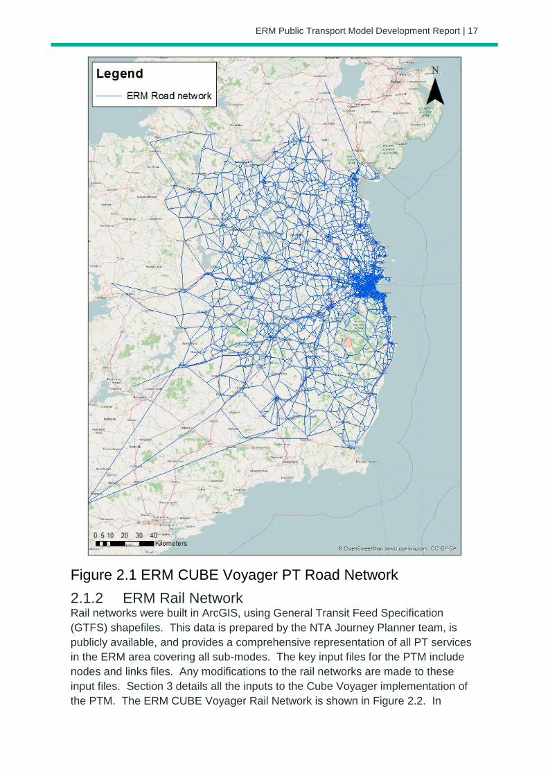
2.1.1 ERM Road Network Within the overall ERM, the primary network is stored as a SATURN road model
network. This is then converted into Cube Voyager format for each time period
whenever the full model is run. The conversion process translates node
coordinates, links distances, capacity indexes, bus lanes and congested speeds
into Cube Voyager format for use in the PT Model. The ERM CUBE Voyager PT
Road Network is shown in Figure 2.1.
Bus speeds in the PT Model are calculated as part of this process depending on
whether there is a bus lane coded on the link or not. Where a bus lane exists on a
link, the bus speed is taken as the car speed on an uncongested assignment, to
take account of signalised junction delays. Where no bus lane exists on the link,
the bus speed is calculated as the assigned network congested speed. A link
category based factor was calibrated to match journey time data during the
calibration process. The final values are provided inTable 4.8 later in this report.
ERM Public Transport Model Development Report | 17
Figure 2.1 ERM CUBE Voyager PT Road Network
2.1.2 ERM Rail Network Rail networks were built in ArcGIS, using General Transit Feed Specification
(GTFS) shapefiles. This data is prepared by the NTA Journey Planner team, is
publicly available, and provides a comprehensive representation of all PT services
in the ERM area covering all sub-modes. The key input files for the PTM include
nodes and links files. Any modifications to the rail networks are made to these
input files. Section 3 details all the inputs to the Cube Voyager implementation of
the PTM. The ERM CUBE Voyager Rail Network is shown in Figure 2.2. In

ERM Public Transport Model Development Report | 18
accordance with the ERM repeatable methods guidance, the network extends to
one stop beyond the limit of the model area. All services were coded to stop at this
first stop outside of the modelled area to ensure that flows entering the model area
are loaded onto the correct services. For example, all services from Dublin to Cork
were coded to stop at Templemore, and a centroid connector from Cork to
Templemore included, so that rail trips from Cork to Dublin enter the model area on
this rail corridor.
Figure 2.2: ERM Rail network
ERM Public Transport Model Development Report | 19
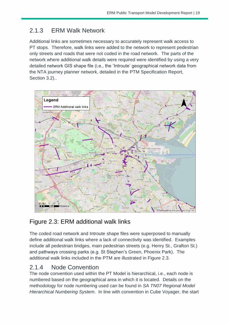
2.1.3 ERM Walk Network
Additional links are sometimes necessary to accurately represent walk access to
PT stops. Therefore, walk links were added to the network to represent pedestrian
only streets and roads that were not coded in the road network. The parts of the
network where additional walk details were required were identified by using a very
detailed network GIS shape file (i.e., the ‘Introute’ geographical network data from
the NTA journey planner network, detailed in the PTM Specification Report,
Section 3.2)..
Figure 2.3: ERM additional walk links
The coded road network and Introute shape files were superposed to manually
define additional walk links where a lack of connectivity was identified. Examples
include all pedestrian bridges, main pedestrian streets (e.g. Henry St., Grafton St.)
and pathways crossing parks (e.g. St Stephen’s Green, Phoenix Park). The
additional walk links included in the PTM are illustrated in Figure 2.3.
2.1.4 Node Convention The node convention used within the PT Model is hierarchical, i.e., each node is
numbered based on the geographical area in which it is located. Details on the
methodology for node numbering used can be found in SA TN07 Regional Model
Hierarchical Numbering System. In line with convention in Cube Voyager, the start

ERM Public Transport Model Development Report | 20
of the node numbering system is reserved for zone numbers (i.e. zone numbers
are numbered sequentially, starting from 1). Following this, Road, Rail, Luas and
Walk nodes have pre-defined ranges of node numbers, and headroom was left to
add extra network in coding any future year transport schemes. The numbering of
Road Network nodes provides a consistency between the Public Transport and
Road Models.
The following node convention has been adopted for the ERM PT network:
1 to 1,999: Zones;
2,000 to 39,999: Road network nodes inside the GDA;
99,000 to 99,499: Rail network nodes;
99,500 to 99,599: Luas Green line nodes (including CrossCity);
99,600 to 99,699: Luas Red line nodes;
99,900 to 99,999: Walk/Cycle network nodes;
99,700 – 99,900: Spare / Scheme coding; and
>99,999: Road network nodes outside the GDA.
2.1.5 Initial Zone Centroid Convention As detailed in the PTM Specification Report (section 3.9.1), initially zone centroid
positions and connector locations were inherited from the road model. This was
later revised during calibration to provide an improved representation of PT travel
costs, as detailed in Section 4.3.3 below.
2.1.6 Non-Transit Legs Access to the PT network is provided by non-transit legs. Non-transit legs are
minimum-cost segments, traversed by non-mechanized modes. They are
generated by the Cube Voyager program to represent any leg of a route not
undertaken on a PT service.
There are four types of zone centroid non-transit leg. In each case the initial
values have been taken from an early calibration of the ERM; these were
subsequently revised as part of the PT Model network and parameter calibration
described in Section 4.4.2.
1) Zone centroid to PT stop access by walk. Walking is the most frequently used mode of access and egress to PT
services. It is limited to 30 minutes with a maximum of 5 legs by zone
centroid/by mode (10 for modes 4 and 5, corresponding to buses).
2) Zone centroid to PT stop access by driving. This allows for access to a PT stop in areas where walk access would be
too long or impractical – this applies especially in rural areas where zones
are larger and PT supply is sparse. The access by drive links correspond
to a “kiss and ride” for PT users – i.e. PT users being dropped off by car at
PT stops. A 30 minutes penalty is applied to these legs to ensure that the
walk access leg is preferred for all short distance access
ERM Public Transport Model Development Report | 21
3) Zone-to-zone access legs. The PT Model requires all PT trips to board at least one PT service.
However, for zones located near to each other where there is limited
network detail this can result in inconsistent routes and high generalised
costs. This causes a problem for the demand model. Zone-to-zone direct
access is therefore included as a non-transit leg. This allows walk trips
between two zones if the cost is less than the cost of using PT between
these zones. This ensures generalised costs increase consistently with
distance. Initially this value was limited to a 10 minute walk, with the cost
of this multiplied by a weight of 2 based on an initial review of short
distance trips within the model. Zone-to-zone direct access was
investigated further during model calibration as detailed in Section 4.4.2
later in this report.
4) Stop-to-stop transfer legs. In addition to the three zone centroid non transit legs, there is a fourth type
of non-transit leg: stop-to-stop transfer legs. These correspond to transfer
walking legs between two transit legs. Initially, they were limited to a 20
minute walk.
2.2 Public Transport Services Preparation
2.2.1 Overview This section details the input data used and conventions adopted in the coding of
PT Services in Cube Voyager software. As per Section 3.9.2 of the PTM
Specification Report, service patterns were defined based on GTFS data.
2.2.2 System Data Cube Voyager requires additional ‘system data’ information for each service, such
as mode, operator, and details of the fare system. The ERM PTM includes the
following modes of transport:
1 – DART
2 – Other Rail
3 – Light Rail
4 – Dublin Bus
5 – Other Bus
6 – BRT (not used in the base year)
7 – Metro (not used in the base year)
It also includes the following operators:
1 – DART
3 – Luas
4 – Dublin Bus
5 – Bus Eireann
6 to 62 – Private Operators
ERM Public Transport Model Development Report | 22
100 to 102 – Irish Rail (1 operator defined by corridor)
104 – Dublin Bus, Airport services
105 – Bus Eireann, Airport services
106 to 149 – Private Operators, Airport services
150 – BRT operator (not used in the base year)
151 – Metro operator (not used in the base year)
All Irish Rail services were initially defined with a single operator (number 2).
However, in order to more accurately represent model fares, it was necessary to
split the services by main corridor of travel i.e. Sligo line, Dundalk-Rosslare and
Southwest. Different operator categories have to be defined for airport services to
allow for different airport fare systems.
2.2.3 Conversion from GTFS to Cube Voyager PT Service Code
The GTFS process outlined in Section 3.9.2 of the PTM Specification Report was
used to convert GTFS data to Cube Voyager PT service coding – i.e. conversion to
PT lines files. Although it is an automatic process, manual adjustments were
required to modify some routes, e.g. to match road network structure or to fill gaps
in the GTFS route definition.
The earliest ‘complete’ set of GTFS data that was available for this conversion was
from February 2014. There was insufficient information available to identify which
services in the 2014 dataset should be considered as invalid for inclusion in a 2012
base model. In the absence of this information, it was decided to use all of the
February 2014 data, and to supplement it where necessary if some routes which
weren’t included in GTFS were identified. These routes included:
Ardcavan Coach Tours: Wellington Bridge to Dublin Airport;
Finlays Coach Hire: Dundalk to NUI Maynooth;
Finlays Coach Hire: Drogheda to NUI Maynooth;
Finlays Coach Hire: NUI Maynooth to Dundalk;
Finlays Coach Hire: Ardee to DKIT;
Finlays Coach Hire: DKIT to Ardee;
Streamline Coaches: Cavan to NUI Maynooth;
Streamline Coaches: NUI Maynooth to Cavan;
Slevins Coaches: Dundrum to NUI Maynooth;
Slevins Coaches:Templeogue to NUI Maynooth;
Slevins Coaches:NUI Maynooth to Dundrum;
OK Transport: Edenderry to NUI Maynooth;
OK Transport: NUI Maynooth to Edenderry;
OK Transport: Allenwood to NUI Maynooth;
OK Transport: NUI Maynooth to Allenwood;
Silver Dawn Travel: Portarlington to UCD; and
Silver Dawn Travel: UCD to Portarlington.
ERM Public Transport Model Development Report | 23
On completion of the GTFS conversion process, a total of 1,053 lines were coded
in the ERM PT Model, split across three lines files, one for bus services, one for rail
services and one for services on new modes (empty in the base year).
The distribution of services across different operators is provided below:
DART: 17 services;
Rail: 61 services;
Luas: 15 services;
Dublin Bus: 342 services;
Bus Éireann: 332 services; and
Other buses: 286 services.
Modelled headways are based on the number of services that operate in each time
period (i.e. 0700 – 1000, 1000 – 1300 and 1600 – 1900) with the time period
definition based on the timetable mid-point within the model network.
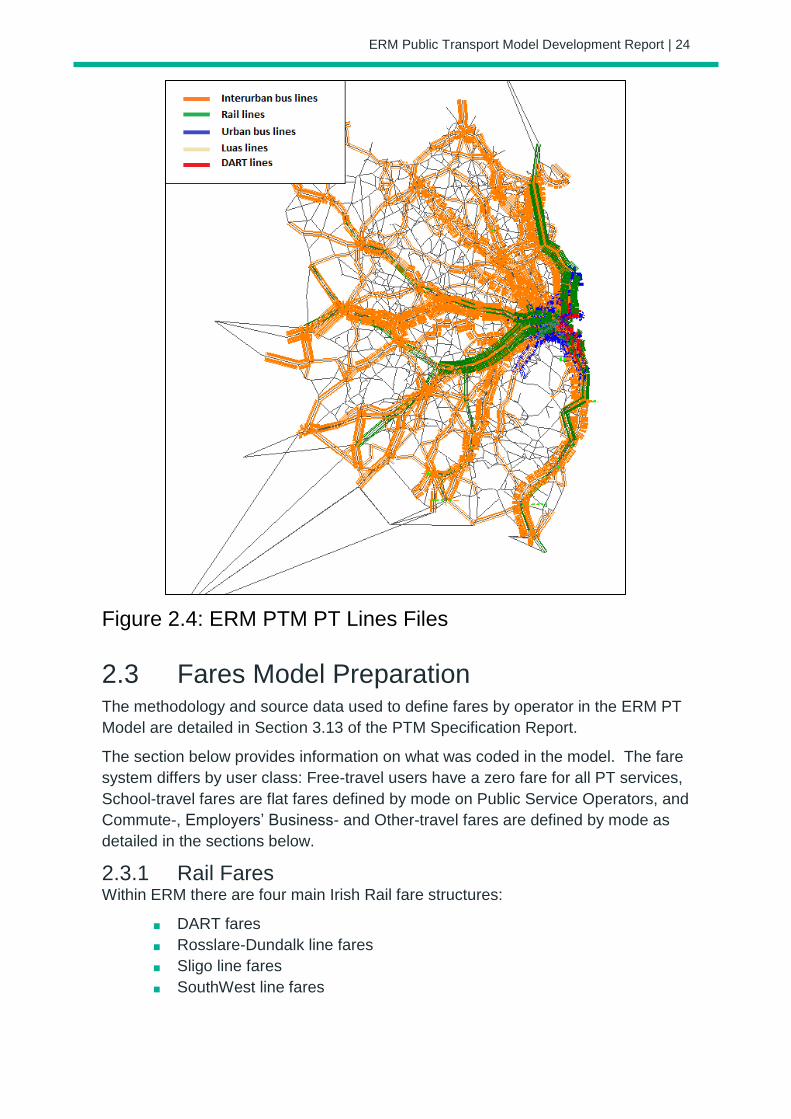
The PT Lines Files for the ERM PTM represents the coded public transport
services for rail, inter urban bus routes, urban bus, Luas and DART routes as
illustrated in Figure 2.4.
ERM Public Transport Model Development Report | 24
Figure 2.4: ERM PTM PT Lines Files
2.3 Fares Model Preparation The methodology and source data used to define fares by operator in the ERM PT
Model are detailed in Section 3.13 of the PTM Specification Report.
The section below provides information on what was coded in the model. The fare
system differs by user class: Free-travel users have a zero fare for all PT services,
School-travel fares are flat fares defined by mode on Public Service Operators, and
Commute-, Employers’ Business- and Other-travel fares are defined by mode as
detailed in the sections below.
2.3.1 Rail Fares Within ERM there are four main Irish Rail fare structures:
DART fares
Rosslare-Dundalk line fares
Sligo line fares
SouthWest line fares
ERM Public Transport Model Development Report | 25
Fares for intercity services are based on four categories associated with
approximate distance travelled, along with service quality i.e. Express, Economy 1
and Economy 2 services.
In the ERM PTM, Irish Rail fares are modelled using a distance based fare system.
This method is more flexible than a fixed fare matrix (between OD stations). It
allows the model itself to calculate distances and is more flexible when
implementing future schemes (i.e., a new railway station added to the network).
Fares and ticket sales information for 2012 were obtained from the NTA, for the top
100 Irish Rail InterCity OD routes based on demand. The information included
single, return, open return, weekly, monthly and annual ticket sales data. This data
was then filtered for stations which are included in the ERM area.
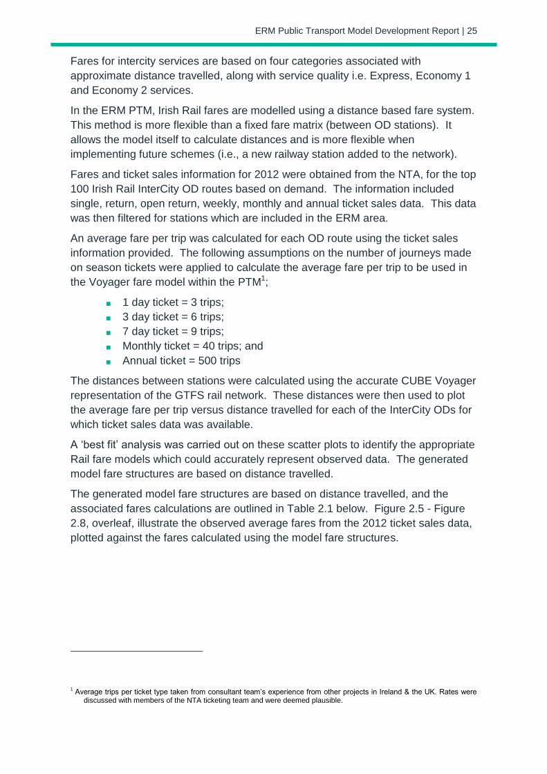
An average fare per trip was calculated for each OD route using the ticket sales
information provided. The following assumptions on the number of journeys made
on season tickets were applied to calculate the average fare per trip to be used in
the Voyager fare model within the PTM1;
1 day ticket = 3 trips;
3 day ticket = 6 trips;
7 day ticket = 9 trips;
Monthly ticket = 40 trips; and
Annual ticket = 500 trips
The distances between stations were calculated using the accurate CUBE Voyager
representation of the GTFS rail network. These distances were then used to plot
the average fare per trip versus distance travelled for each of the InterCity ODs for
which ticket sales data was available.
A ‘best fit’ analysis was carried out on these scatter plots to identify the appropriate
Rail fare models which could accurately represent observed data. The generated
model fare structures are based on distance travelled.
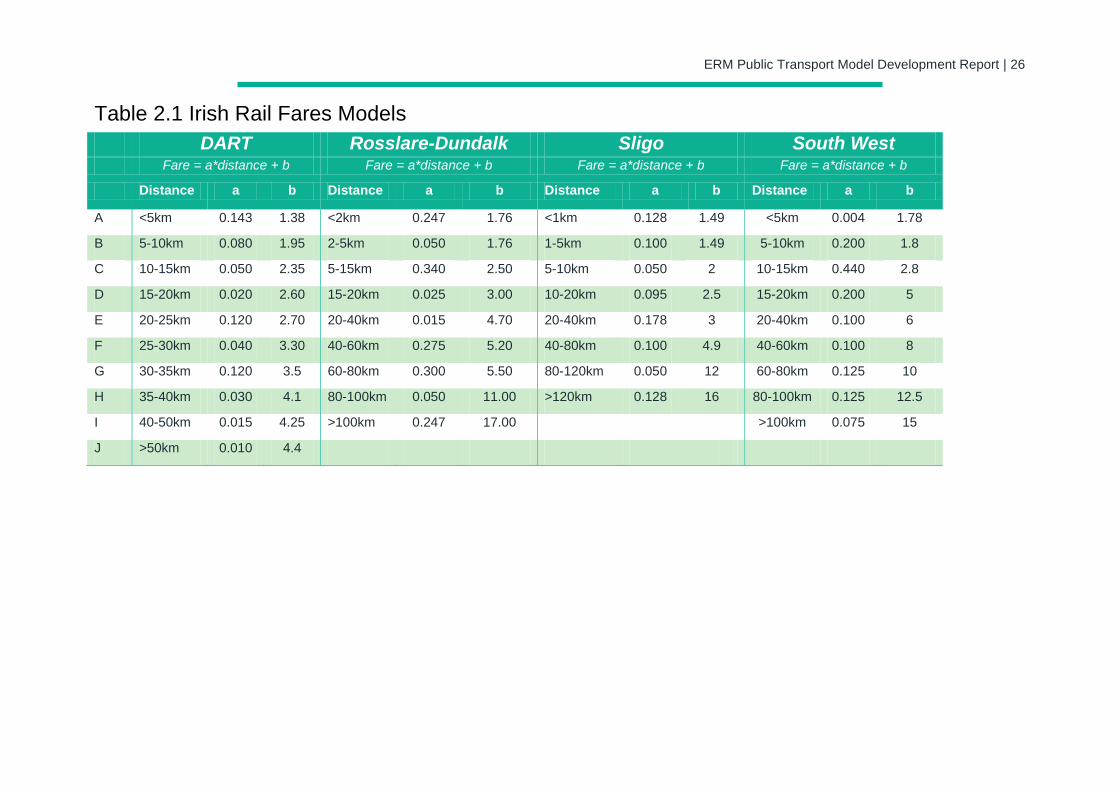
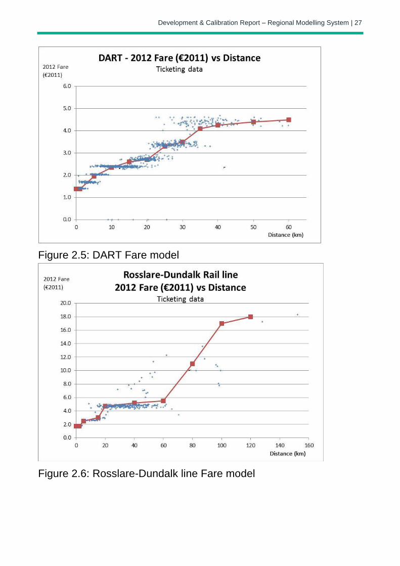
The generated model fare structures are based on distance travelled, and the
associated fares calculations are outlined in Table 2.1 below. Figure 2.5 - Figure
2.8, overleaf, illustrate the observed average fares from the 2012 ticket sales data,
plotted against the fares calculated using the model fare structures.
1 Average trips per ticket type taken from consultant team’s experience from other projects in Ireland & the UK. Rates were
discussed with members of the NTA ticketing team and were deemed plausible.
ERM Public Transport Model Development Report | 26
Table 2.1 Irish Rail Fares Models
DART Rosslare-Dundalk Sligo South West Fare = a*distance + b Fare = a*distance + b Fare = a*distance + b Fare = a*distance + b
Distance a b Distance a b Distance a b Distance a b
A <5km 0.143 1.38 <2km 0.247 1.76 <1km 0.128 1.49 <5km 0.004 1.78
B 5-10km 0.080 1.95 2-5km 0.050 1.76 1-5km 0.100 1.49 5-10km 0.200 1.8
C 10-15km 0.050 2.35 5-15km 0.340 2.50 5-10km 0.050 2 10-15km 0.440 2.8
D 15-20km 0.020 2.60 15-20km 0.025 3.00 10-20km 0.095 2.5 15-20km 0.200 5
E 20-25km 0.120 2.70 20-40km 0.015 4.70 20-40km 0.178 3 20-40km 0.100 6
F 25-30km 0.040 3.30 40-60km 0.275 5.20 40-80km 0.100 4.9 40-60km 0.100 8
G 30-35km 0.120 3.5 60-80km 0.300 5.50 80-120km 0.050 12 60-80km 0.125 10
H 35-40km 0.030 4.1 80-100km 0.050 11.00 >120km 0.128 16 80-100km 0.125 12.5
I 40-50km 0.015 4.25 >100km 0.247 17.00 >100km 0.075 15
J >50km 0.010 4.4
Development & Calibration Report – Regional Modelling System | 27
Figure 2.5: DART Fare model
Figure 2.6: Rosslare-Dundalk line Fare model

ERM Public Transport Model Development Report | 28
Figure 2.7: Sligo Line Fare model
Figure 2.8: Southwest line Fare model
ERM Public Transport Model Development Report | 29
The average fares (from observed 2012 ticket sales data) for each of the four fare
structures (outlined in Table 2.1) were compared against those calculated using the new
fares model, and the results are presented in Table 2.2 below. The results indicate that
the modelled fares provide a good representation of observed fare data with greater than
85% of ODs, for which ticketing data was available, having a modelled fare of between +/-
25% observed values.
Table 2.2 Modelled vs Observed Average Fares
Validation Band % ODs within Validation Bands
DART Rosslare -
Dundalk
Sligo South West
<-50% 0% 2% 0% 0%
Btw -50% & -25% 1% 8% 3% 0%
Btw -25% & +25% 99% 85% 95% 87%
Btw -25% & +50% 0% 2% 1% 7%
> +50% 0% 3% 0% 7%
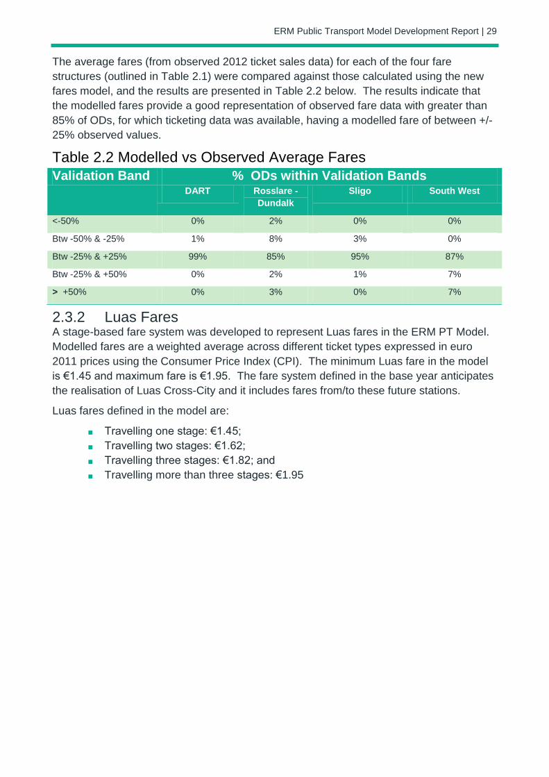
2.3.2 Luas Fares A stage-based fare system was developed to represent Luas fares in the ERM PT Model.
Modelled fares are a weighted average across different ticket types expressed in euro
2011 prices using the Consumer Price Index (CPI). The minimum Luas fare in the model
is €1.45 and maximum fare is €1.95. The fare system defined in the base year anticipates
the realisation of Luas Cross-City and it includes fares from/to these future stations.
Luas fares defined in the model are:
Travelling one stage: €1.45;
Travelling two stages: €1.62;
Travelling three stages: €1.82; and
Travelling more than three stages: €1.95
ERM Public Transport Model Development Report | 30
Figure 2.9: Luas fare system stages
2.3.3 Dublin Bus Fares 2013 ticket sales and revenue data for Dublin Bus services was obtained from the NTA.
This included information on all ticket types, including; singles, returns, day saver, 10
journey etc., and season products including TaxSaver tickets.
This data was used to calculate an approximate weighted average fare per trip for Dublin
Bus services. As outlined for Irish Rail above, a number of assumptions were made
regarding the number of trips made on season tickets to calculate an approximate fare per
trip.
A weighted average fare was calculated for each Dublin Bus fare band and this is applied
as a stage based fare system within CUBE. The City Centre Fare (a lower flat fare if
travelling within a defined central area) is also represented in the model. The Dublin Bus
fares defined in the model are as follows:
City Centre Fare: €0.58;
Travelling 1 to 3 stages: €1.40;
Travelling 4 to 7 stages: €1.87;
Travelling 8 to 13 stages: €2.02; and
Travelling more than 13 stages: €2.28.
ERM Public Transport Model Development Report | 31
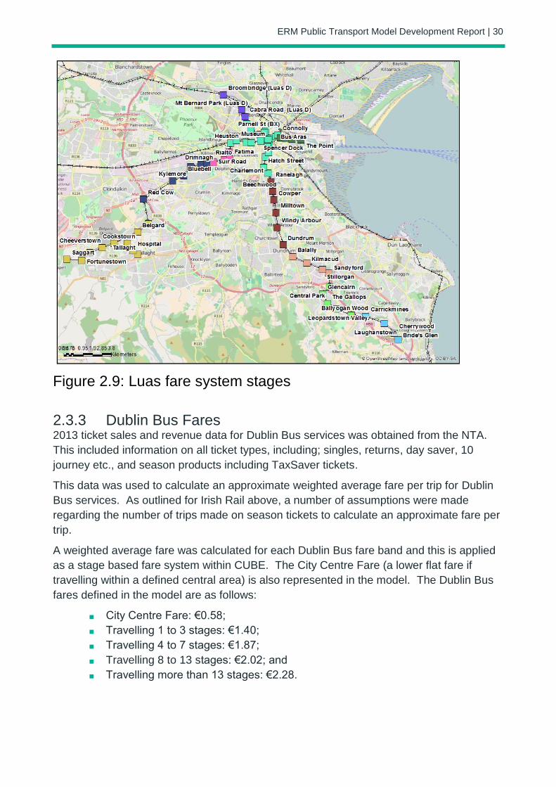
2.3.4 Bus Éireann Fares A distance based fare model was built for application to all Bus Éireann services based on
ticket sales revenue and journey data available on key routes. Below is a plot of 2013
average fares versus distance for a sample of 30 Dublin commuting journeys. The red
curve is the modelled distance fare, which was converted to 2012 fares in 2011 prices to
be consistent with other fare systems.
Figure 2.10 Bus Eireann Fare Model
2.3.5 Private Operator Fares A similar approach to the Bus Éireann fare definition was used to model private operator
fares. All such fares are represented using a single ‘private operator’ fare model. The
steps in developing this model were:
Collect fare data from the private operator websites;
Build a list of Origin-Destination records with fare and distance information;
Plot the data on a Fare Vs. Distance chart; and
Build a distance-based fare model to fit the data.
As ticket sales and revenue data are not available for private operators, this model was
based on single ticket fares. To take account of cheaper fares (season tickets, return
tickets, etc.), private operator fares are factored by 0.83 (this factor was calculated using
average fares / single fares ratio from Public Service Operators).
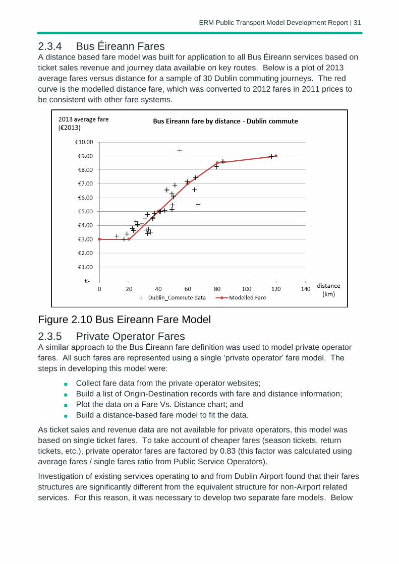
Investigation of existing services operating to and from Dublin Airport found that their fares
structures are significantly different from the equivalent structure for non-Airport related
services. For this reason, it was necessary to develop two separate fare models. Below
ERM Public Transport Model Development Report | 32
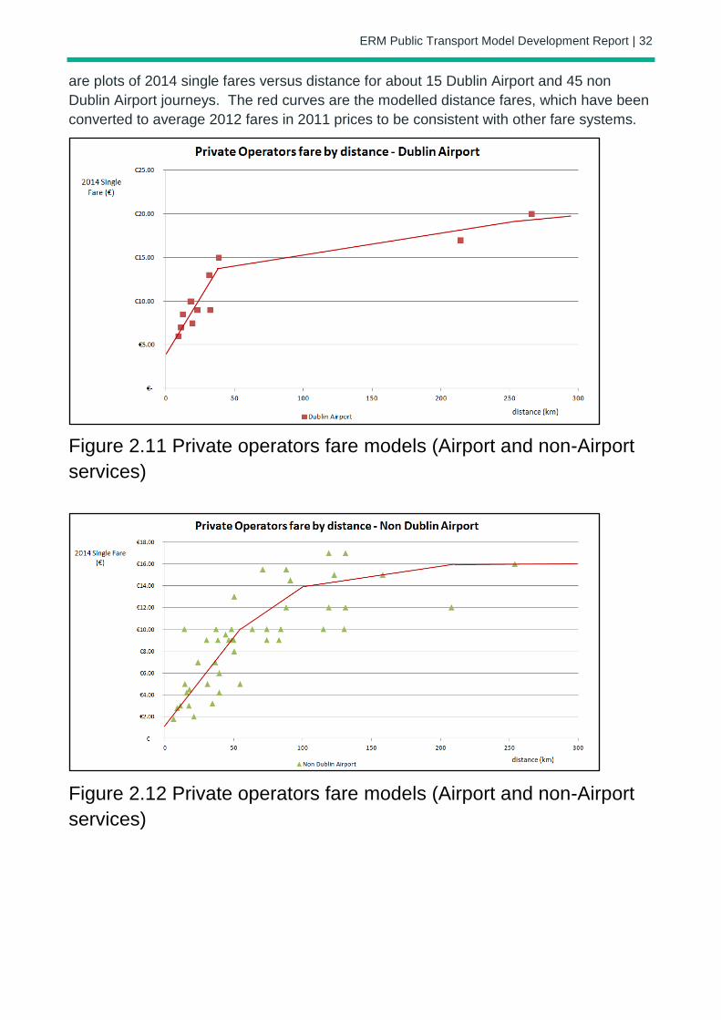
are plots of 2014 single fares versus distance for about 15 Dublin Airport and 45 non
Dublin Airport journeys. The red curves are the modelled distance fares, which have been
converted to average 2012 fares in 2011 prices to be consistent with other fare systems.
Figure 2.11 Private operators fare models (Airport and non-Airport
services)
Figure 2.12 Private operators fare models (Airport and non-Airport
services)
ERM Public Transport Model Development Report | 33
2.3.6 Transfer fares Transfer fares between modes were defined to represent combined tickets for multi-modal
users in the model. Based on pre-paid TaxSavers data, an average 31% fare reduction
has been calculated for users of at least two of the three modes (Rail, Luas, and Dublin
Bus). Assuming that 50% of the users can benefit from that reduction, a flat reduction of
15% of the cheapest fare of the mode was applied to users transferring between Public
Service Operators. No transfer fare reduction was applied in the case of private operators.
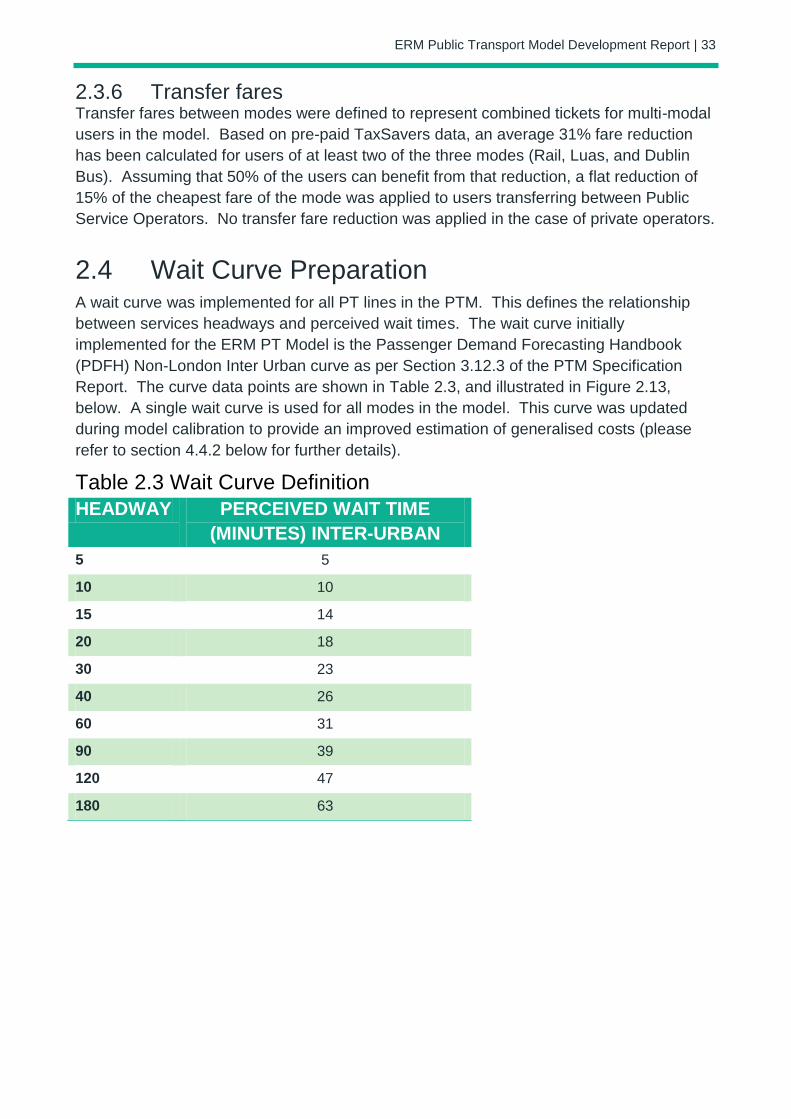
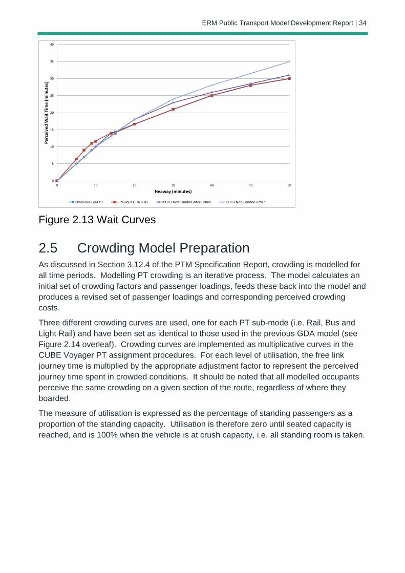
2.4 Wait Curve Preparation A wait curve was implemented for all PT lines in the PTM. This defines the relationship
between services headways and perceived wait times. The wait curve initially
implemented for the ERM PT Model is the Passenger Demand Forecasting Handbook
(PDFH) Non-London Inter Urban curve as per Section 3.12.3 of the PTM Specification
Report. The curve data points are shown in Table 2.3, and illustrated in Figure 2.13,
below. A single wait curve is used for all modes in the model. This curve was updated
during model calibration to provide an improved estimation of generalised costs (please
refer to section 4.4.2 below for further details).
Table 2.3 Wait Curve Definition
HEADWAY PERCEIVED WAIT TIME
(MINUTES) INTER-URBAN
5 5
10 10
15 14
20 18
30 23
40 26
60 31
90 39
120 47
180 63
ERM Public Transport Model Development Report | 34
Figure 2.13 Wait Curves
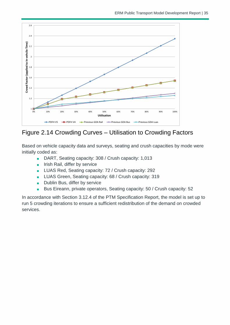
2.5 Crowding Model Preparation As discussed in Section 3.12.4 of the PTM Specification Report, crowding is modelled for
all time periods. Modelling PT crowding is an iterative process. The model calculates an
initial set of crowding factors and passenger loadings, feeds these back into the model and
produces a revised set of passenger loadings and corresponding perceived crowding
costs.
Three different crowding curves are used, one for each PT sub-mode (i.e. Rail, Bus and
Light Rail) and have been set as identical to those used in the previous GDA model (see
Figure 2.14 overleaf). Crowding curves are implemented as multiplicative curves in the
CUBE Voyager PT assignment procedures. For each level of utilisation, the free link
journey time is multiplied by the appropriate adjustment factor to represent the perceived
journey time spent in crowded conditions. It should be noted that all modelled occupants
perceive the same crowding on a given section of the route, regardless of where they
boarded.
The measure of utilisation is expressed as the percentage of standing passengers as a
proportion of the standing capacity. Utilisation is therefore zero until seated capacity is
reached, and is 100% when the vehicle is at crush capacity, i.e. all standing room is taken.
0
5
10
15
20
25
30
35
40
0 10 20 30 40 50 60
Pe
rce
ive
d W
ait
Tim
e (
min
ute
s)
Heaway (minutes)
Previous GDA PT Previous GDA Luas PDFH Non-London inter-urban PDFH Non-London urban
ERM Public Transport Model Development Report | 35
Figure 2.14 Crowding Curves – Utilisation to Crowding Factors
Based on vehicle capacity data and surveys, seating and crush capacities by mode were
initially coded as:
DART, Seating capacity: 308 / Crush capacity: 1,013
Irish Rail, differ by service
LUAS Red, Seating capacity: 72 / Crush capacity: 292
LUAS Green, Seating capacity: 68 / Crush capacity: 319
Dublin Bus, differ by service
Bus Eireann, private operators, Seating capacity: 50 / Crush capacity: 52
In accordance with Section 3.12.4 of the PTM Specification Report, the model is set up to
run 5 crowding iterations to ensure a sufficient redistribution of the demand on crowded
services.
1
1.2
1.4
1.6
1.8
2
2.2
2.4
2.6
0% 10% 20% 30% 40% 50% 60% 70% 80% 90% 100%
Cro
wd
Fac
tor
(ap
plie
d t
o In
-ve
hci
le T
ime
)
Utilisation
PDFH V5 PDFH V4 Previous GDA Rail Previous GDA Bus Previous GDA Luas
ERM Public Transport Model Development Report | 36
3 ERM Cube Voyager Implementation
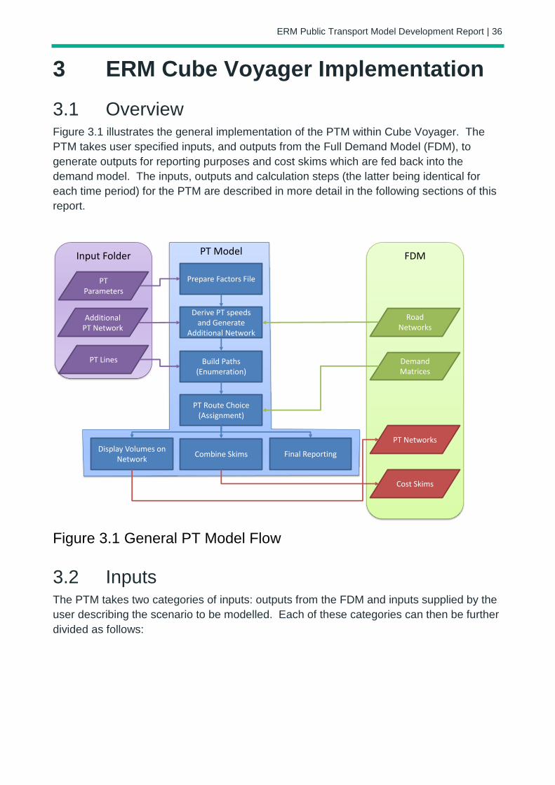
3.1 Overview Figure 3.1 illustrates the general implementation of the PTM within Cube Voyager. The
PTM takes user specified inputs, and outputs from the Full Demand Model (FDM), to
generate outputs for reporting purposes and cost skims which are fed back into the
demand model. The inputs, outputs and calculation steps (the latter being identical for
each time period) for the PTM are described in more detail in the following sections of this
report.
Figure 3.1 General PT Model Flow
3.2 Inputs The PTM takes two categories of inputs: outputs from the FDM and inputs supplied by the
user describing the scenario to be modelled. Each of these categories can then be further
divided as follows:
PT ModelInput Folder
PT Lines
Additional PT Network
PT Parameters
Prepare Factors File
Derive PT speeds and Generate
Additional Network
Build Paths (Enumeration)
PT Route Choice (Assignment)
Display Volumes on Network
Combine Skims Final Reporting
FDM
Road Networks
Demand Matrices
PT Networks
Cost Skims
ERM Public Transport Model Development Report | 37
User Supplied Inputs
network files (which describe the “supply” of public transport, comprising public transport infrastructure and services, including associated infrastructure such as walk connectors, bus lanes and roads along which buses run);
parameters (which control how the model operates); and
analysis files (which specify the reports to be created as the PT model runs).
FDM Outputs
matrices (which contain the demand for public transport services);
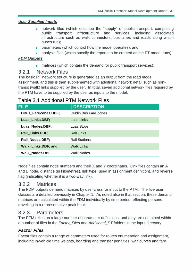
3.2.1 Network Files The basic PT network structure is generated as an output from the road model
assignment, and this is then supplemented with additional network detail such as non-
transit (walk) links supplied by the user. In total, seven additional network files required by
the PTM have to be supplied by the user as inputs to the model:
Table 3.1 Additional PTM Network Files
FILE DESCRIPTION
DBus_FareZones.DBF; Dublin Bus Fare Zones
Luas_Links.DBF; Luas Links
Luas_Nodes.DBF; Luas Stops
Rail_Links.DBF; Rail Links
Rail_Nodes.DBF; Rail Stations
Walk_Links.DBF; and Walk Links
Walk_Nodes.DBF. Walk Nodes
Node files contain node numbers and their X and Y coordinates. Link files contain an A
and B node, distance (in kilometres), link type (used in assignment definition), and reverse
flag (indicating whether it is a two-way link).
3.2.2 Matrices The FDM outputs demand matrices by user class for input to the PTM. The five user
classes are detailed previously in Chapter 1. As noted also in that section, these demand
matrices are calculated within the FDM individually by time period reflecting persons
travelling in a representative peak hour.
3.2.3 Parameters The PTM relies on a large number of parameter definitions, and they are contained within
a number of files in the Factor_Files and Additional_PT folders in the input directory.
Factor Files
Factor files contain a range of parameters used for routes enumeration and assignment,
including In-vehicle time weights, boarding and transfer penalties, wait curves and fare
ERM Public Transport Model Development Report | 38
systems etc. More details on how these parameters operate can be found in the Cube
Voyager Help manual. Separate factor files are defined for each combination of user class
and time period. In addition, a set of additional factor files (one for each time period) is
defined with the suffix ZOD (for Zero Demand). This is used to reduce PT assignment run
times by reducing the level of calculation in the model for OD pairs between which there is
no PT demand.
Fares
The Additional_PT folder contains Fares files which set out the various fare systems to be
utilised within the PTAM for each mode and time period. In addition, PT operators and
modes are defined using a system text file, SYSTEM_FILE.PTS.
Non-Transit Legs
Finally, an external script file, NTL_GENERATE_SCRIPT.txt, is contained in the
Additional PT folder and is read in during a model run. This file is generally not altered.
This script defines various parameters used to build the Non-Transit Legs, such as
maximum number of PT stops a zone can reach by mode or specific PT access for
external zones.
3.2.4 Analysis Files Select links are undertaken during PTM assignment and are defined using a script file (not
a core part of the model but referenced by the true scripts), SELECT_LINK_SPEC.txt.
The select link input file provides a way for the user to input links / lines to be skimmed,
with output matrices added at the end of the cost matrices.
3.3 Network Link Attributes The PT network shares attributes with the road network, but also includes others. Below is
a list of those attributes and their meanings:
Distance: Link distance in kilometres;
CI: Capacity Index - dumped from the road network;
Bus_Lanes: Indicator whether a bus lane is coded on the link (=1) or not (=0) -
dumped from the road network;
Link_Type: Attribute to identify the main role of the link as follows:
1 – Road link
25 – Walk only link
27 – Rail / Luas link
31 – Zone connector to the road network
32 – Zone connector to the rail network
Crosscity: Indicates whether the link is part of the Luas crosscity extension (=1)
or not (=0).
ERM Public Transport Model Development Report | 39
3.4 Key Parameters Key parameters are outlined in Section 3.12 of the PTM Specification Report, and include:
Route enumeration controls – these determine the spread of routes that are
taken forward to evaluation and the more detailed assignment stage;
Boarding & Interchange Penalties – these relate not only to service reliability
but also to the provision of facilities at boarding points, such as waiting facilities,
information and security. These may relate to future proposed network
enhancements;
In-vehicle weights by modal preference factors – associated with the relative
comfort and perception of travel time in different modes, or different vehicle
types; and
Wait Curves and Factors - these relate service frequencies to the actual
perceived wait time experienced by passengers. This is especially important
when journeys involve interchange and services of differing frequencies, for
example interchange between rail and bus services.
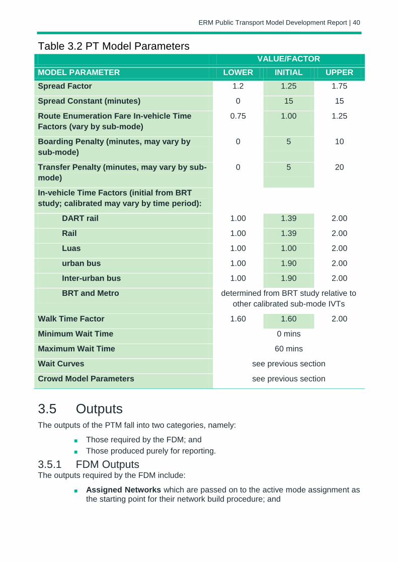
Table 3.2 below outlines the range of initial values for parameters used to set up the PT
Model.
ERM Public Transport Model Development Report | 40
Table 3.2 PT Model Parameters VALUE/FACTOR
MODEL PARAMETER LOWER INITIAL UPPER
Spread Factor 1.2 1.25 1.75
Spread Constant (minutes) 0 15 15
Route Enumeration Fare In-vehicle Time
Factors (vary by sub-mode)
0.75 1.00 1.25
Boarding Penalty (minutes, may vary by
sub-mode)
0 5 10
Transfer Penalty (minutes, may vary by sub-
mode)
0 5 20
In-vehicle Time Factors (initial from BRT
study; calibrated may vary by time period):
DART rail 1.00 1.39 2.00
Rail 1.00 1.39 2.00
Luas 1.00 1.00 2.00
urban bus 1.00 1.90 2.00
Inter-urban bus 1.00 1.90 2.00
BRT and Metro determined from BRT study relative to
other calibrated sub-mode IVTs
Walk Time Factor 1.60 1.60 2.00
Minimum Wait Time 0 mins
Maximum Wait Time 60 mins
Wait Curves see previous section
Crowd Model Parameters see previous section
3.5 Outputs The outputs of the PTM fall into two categories, namely:
Those required by the FDM; and
Those produced purely for reporting.
3.5.1 FDM Outputs The outputs required by the FDM include:
Assigned Networks which are passed on to the active mode assignment as the starting point for their network build procedure; and

ERM Public Transport Model Development Report | 41
Generalised Cost Matrices by user class for each of the four assigned time periods to be fed back into mode and destination choice. For the unassigned time periods, assumptions are applied to derive approximations of generalised costs as detailed in Chapter 20 of the RM Full Demand Model Specification Report.
3.5.2 Reporting Outputs The PTM produces a number of reporting outputs specifically by time period (in individual
folders). Table 3.3 summarises these outputs.2
Table 3.3 PT Model Outputs
REPORT DESCRIPTION
TP_MATRIX_TOTALS.CSV; Summary of matrix totals
TP_LINK_RECS.DBF; Network links with PT lines data (Count of lines,
services/hour) and assigned trips.
TP_LINK_RECS_PREP.DBF; Network links with PT lines data (Count of lines,
services/hour).
TP_ON_OFFS.DBF; Network links with Boarding and Alighting data by
line.
TP_ON_OFFS_NT.DBF; Network links with Boarding and Alighting (Non
Transit legs only).
TP_ON_OFFS_PREP.DBF; File to prepare the ON_OFFS file
TP_RAIL_B&A.DBF; Total boarding and alighting by node.
TP_RAIL_B&A_SPLIT.DBF; Total boarding and alighting by node and by
mode.
TP_RAIL_LOADINGS.DBF; Rail network links flows by line.
TP_PT_ASSIGNED.LIN; Line file with volume information.
TP_PT_COMPCST.MAT; PT Composite Costs matrices for all user classes.
TP_PT_EMP.MAT; Detailed components of PT costs for UC
Employers Business.
TP_PT_COM.MAT; Detailed components of PT costs for UC
Commute.
TP_PT_RET.MAT; Detailed components of PT costs for UC Free
Travel.
TP_PT_OTH.MAT; Detailed components of PT costs for UC Other.
TP_PT_EDU.MAT; Detailed components of PT costs for UC
Education.
2 The TP indicates a time period variable and can take the values AM, LT, SR, and PM.
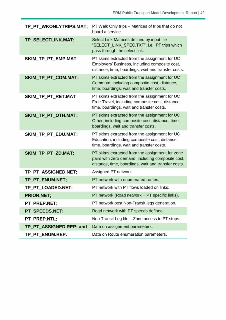
ERM Public Transport Model Development Report | 42
TP_PT_WKONLYTRIPS.MAT; PT Walk Only trips – Matrices of trips that do not
board a service.
TP_SELECTLINK.MAT; Select Link Matrices defined by input file
“SELECT_LINK_SPEC.TXT”, i.e., PT trips which
pass through the select link.
SKIM_TP_PT_EMP.MAT PT skims extracted from the assignment for UC
Employers’ Business, including composite cost,
distance, time, boardings, wait and transfer costs.
SKIM_TP_PT_COM.MAT; PT skims extracted from the assignment for UC
Commute, including composite cost, distance,
time, boardings, wait and transfer costs.
SKIM_TP_PT_RET.MAT PT skims extracted from the assignment for UC
Free-Travel, including composite cost, distance,
time, boardings, wait and transfer costs.
SKIM_TP_PT_OTH.MAT; PT skims extracted from the assignment for UC
Other, including composite cost, distance, time,
boardings, wait and transfer costs.
SKIM_TP_PT_EDU.MAT; PT skims extracted from the assignment for UC
Education, including composite cost, distance,
time, boardings, wait and transfer costs.
SKIM_TP_PT_ZD.MAT; PT skims extracted from the assignment for zone
pairs with zero demand, including composite cost,
distance, time, boardings, wait and transfer costs.
TP_PT_ASSIGNED.NET; Assigned PT network.
TP_PT_ENUM.NET; PT network with enumerated routes.
TP_PT_LOADED.NET; PT network with PT flows loaded on links.
PRIOR.NET; PT network (Road network + PT specific links).
PT_PREP.NET; PT network post Non-Transit legs generation.
PT_SPEEDS.NET; Road network with PT speeds defined.
PT_PREP.NTL; Non Transit Leg file – Zone access to PT stops.
TP_PT_ASSIGNED.REP; and Data on assignment parameters.
TP_PT_ENUM.REP. Data on Route enumeration parameters.
ERM Public Transport Model Development Report | 43
4 PT Model Calibration
4.1 Introduction This chapter describes the process of calibration of the PTM, while Chapter 5 outlines the
results of the PTM validation. In conventional modelling theory, these are two separate
processes. Model calibration is the process of adjusting model parameters and inputs to
ensure the model outputs match observed data as closely as possible. Model validation is
the process of comparing the outputs of the calibrated model against a separate set of
observed data not used in the calibration process. In practice, however, the two
processes are interlinked in that issues identified during validation stage can be addressed
by modifying calibration parameters.
PT Model calibration followed an iterative process, where improvements to the PT model
led to better costs, which fed into the Demand Model, which in turn was improved to
produce better estimates of PT demand. The Demand Model calibration process is
described in ERM Demand Model Calibration Report.
4.2 Assignment Calibration Process
4.2.1 Overview Calibration is the process of adjusting the PT Model to ensure it provides robust estimates
of sub-mode choice, assignment and generalised cost before integrating it into the full
ERM. This is typically achieved in iteration with the validation of the model to independent
data. For the ERM, assignment calibration was undertaken through comparisons of model
outputs and observed data for the following:
Passenger Flows;
Boardings and Alightings;
Bus Journey Times; and
Interchanges.
The UK’s Department for Transport’s Transport Analysis Guidance (TAG) unit M3-2 PT
assignment modelling, January 2014, indicates that the assignment model may be
recalibrated by one or more of the following means:
adjustments may be made to the zone centroid connector times, costs and
loading points;
adjustments may be made to the network detail, and any service
amalgamations in the interests of simplicity may be reconsidered;
the in-vehicle time factors may be varied;
the values of walking and waiting time coefficients or weights may be varied;
the interchange penalties may be varied;
the parameters used in the trip loading algorithms may be modified;
the path building and trip loading algorithms may be changed; and
the demand may be segmented by person (ticket) type.

ERM Public Transport Model Development Report | 44
TAG indicates that the above suggestions are generally in the order in which they should
be considered, however, this is not an exact order of priority but a broad hierarchy that
should be followed. In all cases, any adjustments must remain plausible and should be
based on a sound evidence base.
Calibration is broadly split into three components discussed in the following sections of this
chapter, namely, adjustments to:
PT Network;
PT Parameters; and
PT Matrices.
4.3 PT Model Network Progression
4.3.1 Overview The development of the initial PT network, services and fares model has already been
described in Chapter 2. Following this, two types of checks were carried out:
Non Transit Leg PT Access Testing: To ensure levels of access to PT
services were represented correctly for all zones in the PTM; and
PT Generalised Cost Checks: To ensure the costs generated by the PT
model would not cause problems during the calibration of the demand model.
For example, large PT costs could lead to insensitive generalised cost
parameters estimated during calibration. This may impact on the model’s
sensitivity to future PT scheme changes
4.3.2 Non Transit Leg PT Access Testing Every model zone is assigned to a ‘zone centroid’ network node. PT trips to/from a zone
begin and end at the centroid to access the main PT and/or road network via a centroid
connector by walking.
The actual distances walked from locations within a zone boundary and the actual network
within that zone can vary substantially (and this variance is in proportion to the zone size).
Ideally the centroid connector length is chosen so as to minimise this variance for all trips,
but since not all trips are observed, a general rule for connector length is usually applied.
This can result in long connectors (and hence long walks) between the locations of trip
origins/destinations, (abstractly represented by centroids), and the nearest PT services.
In order to identify any issues with access to PT services within the PTM, analysis was
undertaken of the time taken to get from from each zone centroid to the nearest PT stop
for each of the following sub-modes:
DART;
Intercity Rail;
Luas;
Dublin Bus; and
Bus Éireann

ERM Public Transport Model Development Report | 45
The analysis involved identifying the minimum walk or driving time from each zone to
access the nearest PT stop, for each sub-mode, using the modelled lines derived from
GTFS and the network taken directly from the road model.
No account was taken of the other journey characteristics that would be considered in a
full PT assignment, including headways, transit times and fares.
Internal zones had walk or drive access to all PT modes except for urban bus services
(Dublin Bus), which were only accessible by walk. Access by car was capped to 30
minutes drive. The perceived cost for motorised access included a 30 minutes penalty,
and this was multiplied by a factor of 2. For walk access, the assumed walk speed was
4.8kph and no walk access routes greater than 40 minutes were included. It should be
noted that these values represent initial assignment parameters prior to model calibration.
These parameters were updated during calibration as detailed in Section 4.4.2 below.
External zones had motorised access only, limited to 200 minutes, and this directly
connected to only the rail and inter urban bus modes.
Figure 4.1 provides a sample illustration of the PT access analysis undertaken for the
ERM. The general finding expected was that zones on PT services would have low access
time, with zones more distant from such services having correspondingly higher access
times. Any zone (or set of zones) which contradicted this expectation was investigated for
connectivity issues (e.g. missing centroid connectors or lack of PT network/service coding)
and then corrected.
Figure 4.1 Non-Transit Leg PT Access Testing

ERM Public Transport Model Development Report | 46
4.3.3 PT Generalised Cost Checks – Network Checks The initial access tests, detailed above, provided a check on the developed PT Network in
terms of access and connectivity to public transport services. It was noted through an
initial assignment of the SWRM, that the developed PT model was generating significantly
high generalised costs which would cause difficulties during calibration of the FDM.
A series of tests were carried out in the SWRM to identify measures which could assist in
producing more realistic PT generalised costs. These tests were primarily undertaken
using the SWRM (and not the ERM) due to quicker run times which allowed numerous
tests to be undertaken in a short period of time. The full set of tests are described in further
detail in Section 4.3 of the SWRM Public Transport Model Development Report. For
completeness, all tests were described in the SWRM report, even though not all changes
were retained in the revised version of the PT Model. Table 4.1 below, provides an
overview of all network tests undertaken on the SWRM including an indicator stating
whether the change was retained or not in the ERM.
Table 4.1 Summary of Generalised Cost Tests carried out in
SWRM
Test Retained?
Zone Disaggregation Retain
Cap PT Cost Connectors Do Not Retain
All Services Make All Stops Do Not Retain
Direct Zone to Stop Connectors Retain
PT Services Reviewed Retain
Cap Centroid Connectors Not Retained in ERM3
It was envisaged that all of the regional models would experience similar problems in
terms of high levels of PT generalised cost. Therefore, alterations from the SWRM which
were found to be beneficial in terms of better representing generalised costs were adopted
for all regions, including the ERM. The following sections provide a brief description of the
changes which were adopted for the ERM on foot of testing carried out in the SWRM PTM.
Zone Disaggregation
In the initial PT assignment, the length of the PT walk connector was taken to be
proportional to the area of the zone (it was taken to be 2/3 of the radius of the zone, with
the approximation that each zone was a perfect circle). This resulted in long walk
connectors, and hence a high PT access cost, for some zones.
3 Zone areas, and corresponding connector distances, are significantly shorter in the ERM when compared to the other regional models that contain large rural areas. As such, the capping of zone connectors was not required in the ERM PT Model.
ERM Public Transport Model Development Report | 47
Where a zone had a walk connector longer than 3km it was flagged for review. For each
of these zones the population density of each of the CSAs making up the zone was
displayed on a map. If there was an area that was more densely populated (usually a
small town or village) this was separated into a new zone, and the surrounding more rural
area left as a separate zone. Further information on the zone disaggregation process is
provided in Chapter 3 of the ERM Zone System Development Report.
Direct Zone to Stop Connectors
The repeatable methods developed for the ERM include a process for revising walk
connectors in areas where the road network is not detailed enough to represent the routes
used by passengers when accessing PT services (see PT TN01 PT Model Walk
Connections technical note for further information). This is mainly an issue in rural areas.
The following approach was adopted for the ERM:
1) All centroids were relocated based on a weighted location of Geo-Directory population and employment.
2) In dense areas where zones are relatively small and there is a detailed representation of the road network, a single connector to the nearest node was coded to replace the connectors inherited from the SATURN model. These are connected to spigots which are often not connected to the nearest node to the centroid. The connector distances were estimated based on crow-fly distance from relocated centroids to the closest node. Crow-fly distances were multiplied by a factor of 1.2. This is a commonly applied factor in Accession4 used to estimate the actual distance walked along a road, taking into account the geometry of the road network which is represented by straight lines in the SATURN model.
3) In other areas where zones are bigger and the modelled network is coarser, possible walk routes are not fully represented, and this can lead to a bus/ rail bias. For example, if a network link was coded from the centroid directly to a train station, whereas there is no direct link from the centroid to the nearest bus stop. In this instance passengers have to walk along modelled links in the highway network to access bus and this may result in more passengers being modelled as using the train due to the lower access time when there is actually a bus stop closer than the train station. To avoid this, the centroids were connected:
a) Directly to all of the GTFS PT stops if they are located less than 2.4km from the zone centroid (crow-fly distance). (This is based on the maximum walk time of 30 minutes and a walk speed of 4.8km/h.)
b) To the nearest node if there is no stop less than 2.4km from the zone centroid (crow-fly distance).
To incorporate these changes within the PTM, all zone centroids connectors inherited from
the highway assignment are automatically deleted. Instead all of the PT connectors are
4 An accessibility analysis software package

ERM Public Transport Model Development Report | 48
included in the Walk_links.dbf input file at the network building stage. The approach
described above required the categorisation of zones based on size, location and network
density to select the appropriate zone connectivity method.
A manual check of the connectors produced was undertaken to ensure they are sensible.
This included consideration of the PT services at each stop to ensure that valid services
are connected, and to retain a single stop on each valid bus corridor by selecting the
minimum distance corridor. Effort was made to remove or amend connections that may
not be possible in reality due to physical barriers, for example rivers or motorways.
PT Services Reviewed
A detailed review was carried out on outputs from the GTFS extraction process. Stopping
sequences for certain lines were updated as some routes weren’t properly coded. In
particular, issues arose where services extended outside the model area (e.g. Dublin-
Limerick) and were not coded as stopping at the edge of the network.
All modelled headways were checked against timetables available online from Bus
Éireann and other service provider websites. Where necessary, headways were updated
to represent as accurately as possible all PT services in the modelled area.
4.3.4 Detailed Network Audit A detailed network audit was completed after all major changes outlined above had been
applied to the model. This identified a number of recommendations that were applied, and
are summarised in the Table 4.2 below:
Table 4.2 Detailed Network Audit Recommendations
Type Description
Network
Services
Rail and bus services leaving and entering the
model updated to have their last stopping node at
the last node of the network
Headways All headways capped at 61 minutes to avoid
capacity issues
External
Connectors
New methodology for calculating lengths of external
connectors
Crowding Headways
The calculation of coded headways is based on the frequency of services from GTFS data
at the period level (i.e. 7-10 in the AM) whereas only the peak hour (60min) is being
assigned.
For a service going only once in the AM period (say at 8.30 AM), a headway of 180min
was initially coded. This resulted in an hourly capacity being divided by three (180/60). In
order to avoid underestimation of supply and inconsistent crowding, the headways were
capped at 61 minutes. The impact of that is a correct hourly capacity for the assigned
ERM Public Transport Model Development Report | 49
peak hour. Nevertheless, the wait time will tend to be underestimated. This is arguable as
a service running only once in the AM period would most likely run within the peak hour,
and therefore, the wait time would probably correspond to that of an hourly service.
The capping of headways can have another drawback if there is a requirement to convert
services into fleet requirement or 24h operating costs. The model inputs are now not able
to differentiate between 60 min or 180 min headway services.
Updated External Connector Distances
External zones are generally connected to motorways and road connectors and don’t
necessary join the network where PT services operate. Zones with no access to PT were
listed, and zone connectors were added for those zones as part of the calibration process.
To represent accurate access costs by Public Transport, a new methodology was
introduced whereby the connector distances were calculated based on the cost of
travelling by sub-mode (i.e. bus and rail) from the centroid connector to a defined
settlement on the edge of the model network.
The cost of travelling by sub-mode was calculated based on:
Distance from the defined zone centroid location to the settlement on the
edge of the model network;
Time of travel based on sub-mode; and
Approximate fare calculated utilising the ERM distance based fare structures
for bus and rail.
The approximate cost of travel was calculated for each connector and PT mode available,
and this was utilised to generate updated connector distances for input into the ERM PTM.
4.4 PT Model Parameters Progression
4.4.1 Initial Parameters Initial PT model parameters were taken from the PTM Specification Report and an early
version of the ERM, and are outlined in Table 3.2 previously, along with an acceptable
range of values.
4.4.2 PT Generalised Cost Checks As part of the PT Generalised Cost checks outlined previously in Section 4.3.3 and
detailed in the SWRM Public Transport Model Development Report, a number of PT
assignment parameters were reviewed and updated. The main changes were made in the
following PT input files:
NTL_GENERATE_SCRIPT.txt: defines the non-transit legs generation
process;
SYSTEM_FILE.pts: defines the mode, operators, wait curves and crowding
curves within the PTM; and
AM_PT_ASS_8.s: Script controlling the PT assignment within CUBE.
ERM Public Transport Model Development Report | 50
As a starting point, the following assignment parameters were defined:
Mode 96: Drive to PT Stop (see Section 2.1.6 for further details)
30 min penalty on connector (no drive time included)
Maximum 60 minutes
Slack of 10 minutes
1 leg by sub-mode, 5 for Inter-Urban Bus
Weight factor: 2
Mode 97: Walk to PT Stop (see Section 2.1.6 for further details)
Maximum 30 minutes
Slack of 10 min
5 legs by sub-mode, 10 for modes 4 and 5, corresponding to
buses
Weight factor: 2
Mode 98: Zone-to-zone walk (see Section 2.1.6 for further details)
Maximum 20 minutes
Pure walk cost
Weight factor: 2
Similar to the network checks outlined previously, a series of tests were carried out in the
SWRM on alterations to PT parameters and their impact on producing improved
generalised costs for calibration. Table 4.3 below provides an overview of all tests
undertaken including an indicator to state whether the proposed change is to be retained
in the ERM. Detailed descriptions of all tests are described in the SWRM Public Transport
Model Development Report.
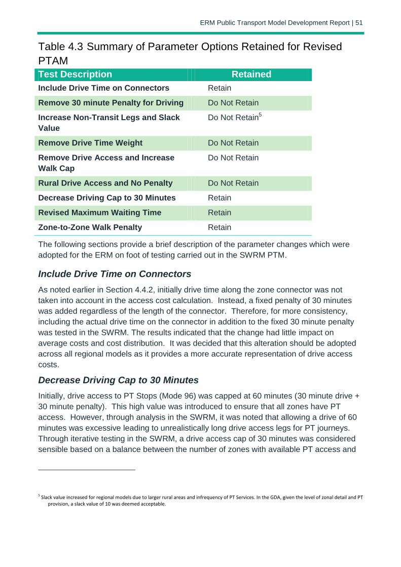
ERM Public Transport Model Development Report | 51
Table 4.3 Summary of Parameter Options Retained for Revised
PTAM
Test Description Retained
Include Drive Time on Connectors Retain
Remove 30 minute Penalty for Driving Do Not Retain
Increase Non-Transit Legs and Slack
Value
Do Not Retain5
Remove Drive Time Weight Do Not Retain
Remove Drive Access and Increase
Walk Cap
Do Not Retain
Rural Drive Access and No Penalty Do Not Retain
Decrease Driving Cap to 30 Minutes Retain
Revised Maximum Waiting Time Retain
Zone-to-Zone Walk Penalty Retain
The following sections provide a brief description of the parameter changes which were
adopted for the ERM on foot of testing carried out in the SWRM PTM.
Include Drive Time on Connectors
As noted earlier in Section 4.4.2, initially drive time along the zone connector was not
taken into account in the access cost calculation. Instead, a fixed penalty of 30 minutes
was added regardless of the length of the connector. Therefore, for more consistency,
including the actual drive time on the connector in addition to the fixed 30 minute penalty
was tested in the SWRM. The results indicated that the change had little impact on
average costs and cost distribution. It was decided that this alteration should be adopted
across all regional models as it provides a more accurate representation of drive access
costs.
Decrease Driving Cap to 30 Minutes
Initially, drive access to PT Stops (Mode 96) was capped at 60 minutes (30 minute drive +
30 minute penalty). This high value was introduced to ensure that all zones have PT
access. However, through analysis in the SWRM, it was noted that allowing a drive of 60
minutes was excessive leading to unrealistically long drive access legs for PT journeys.
Through iterative testing in the SWRM, a drive access cap of 30 minutes was considered
sensible based on a balance between the number of zones with available PT access and
5 Slack value increased for regional models due to larger rural areas and infrequency of PT Services. In the GDA, given the level of zonal detail and PT provision, a slack value of 10 was deemed acceptable.
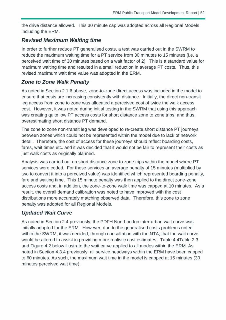
ERM Public Transport Model Development Report | 52
the drive distance allowed. This 30 minute cap was adopted across all Regional Models
including the ERM.
Revised Maximum Waiting time
In order to further reduce PT generalised costs, a test was carried out in the SWRM to
reduce the maximum waiting time for a PT service from 30 minutes to 15 minutes (i.e. a
perceived wait time of 30 minutes based on a wait factor of 2). This is a standard value for
maximum waiting time and resulted in a small reduction in average PT costs. Thus, this
revised maximum wait time value was adopted in the ERM.
Zone to Zone Walk Penalty
As noted in Section 2.1.6 above, zone-to-zone direct access was included in the model to
ensure that costs are increasing consistently with distance. Initially, the direct non-transit
leg access from zone to zone was allocated a perceived cost of twice the walk access
cost. However, it was noted during initial testing in the SWRM that using this approach
was creating quite low PT access costs for short distance zone to zone trips, and thus,
overestimating short distance PT demand.
The zone to zone non-transit leg was developed to re-create short distance PT journeys
between zones which could not be represented within the model due to lack of network
detail. Therefore, the cost of access for these journeys should reflect boarding costs,
fares, wait times etc. and it was decided that it would not be fair to represent their costs as
just walk costs as originally planned.
Analysis was carried out on short distance zone to zone trips within the model where PT
services were coded. For these services an average penalty of 15 minutes (multiplied by
two to convert it into a perceived value) was identified which represented boarding penalty,
fare and waiting time. This 15 minute penalty was then applied to the direct zone-zone
access costs and, in addition, the zone-to-zone walk time was capped at 10 minutes. As a
result, the overall demand calibration was noted to have improved with the cost
distributions more accurately matching observed data. Therefore, this zone to zone
penalty was adopted for all Regional Models.
Updated Wait Curve
As noted in Section 2.4 previously, the PDFH Non-London inter-urban wait curve was
initially adopted for the ERM. However, due to the generalised costs problems noted
within the SWRM, it was decided, through consultation with the NTA, that the wait curve
would be altered to assist in providing more realistic cost estimates. Table 4.4Table 2.3
and Figure 4.2 below illustrate the wait curve applied to all modes within the ERM. As
noted in Section 4.3.4 previously, all service headways within the ERM have been capped
to 60 minutes. As such, the maximum wait time in the model is capped at 15 minutes (30
minutes perceived wait time).

ERM Public Transport Model Development Report | 53
Table 4.4 Wait Curve Definition
Headway Wait Curve Value
(Mins)
Perceived Wait
Time (mins)
5 2.5 5
10 5 10
15 7 14
20 9 18
30 11.5 23
40 13 26
60 15 30
90 17 34
120 18 36
180 20 40
Figure 4.2 Modelled wait curve
4.4.3 Detailed Parameter Audit At the same time as the Detailed Network Audit described in Section 4.3.4, a detailed audit
of parameter values was also conducted. This identified a number of recommendations
that were applied, and are summarised in the Table 4.5 below. More details on the In-
Vehicle Time factors, Walk and Wait Time Factors, Boarding and Interchange penalties
and Load Distribution Factors are given in the following sections.
0
5
10
15
20
25
0 20 40 60 80 100 120 140 160 180 200
ERM Wait Curve
Proposition
Wait time (min)
Headway (min)

ERM Public Transport Model Development Report | 54
Table 4.5 Detailed Parameter Audit Recommendations
Type Description
Non-Transit Legs Revised mode 98 (zone-to-zone) cost: now
estimated with 30min + 2x walk time and
capped at 10 min walk (i.e. a maximum cost of
50 min)
In-Vehicle Time Rail IVT set to 1.3
Bus IVT set to 1.5
LUAS IVT set to 1.0
Walk Time Factor Set to 1.6
Wait Time Factor Set to 2.0
Boarding Penalty Set to 10
Interchange Penalty All Modes to/from DART or Rail = 15
Dublin Bus to Dublin Bus = 15
Other Transfer = 5
Load Distribution
Factor
Set to 50% for coaches in the PTM
In vehicle time factors
In-vehicle time factors are defined for the 5 modes (DART, Other Rail, Luas, Dublin Bus
and Other Bus) to represent relative comfort and perception of travel time. The Calibration
process started with initial values from BRT stated preference research, which have been
refined to improve sub-mode share during model calibration (Table 4.6).
Table 4.6 In-vehicle time factors – initial and calibrated values MODE STATED
PREFERENCE
CALIBRATED
ERM
DART 1.39 1.30
OTHER RAIL 1.39 1.30
LUAS 1.00 1.00
DUBLIN BUS 1.90 1.50
OTHER BUS 1.90 1.50
Walk and wait time factors
Walk time factors represent the discomfort of walking to/ from a transit stop. This value is
applied to the total walk time to/ from a transit stop, including walk time on the zone
ERM Public Transport Model Development Report | 55
centroid connector and on the PT network. WebTAG suggests values between 1.5 and
2.0. A walk time factor of 1.6 was calibrated in the ERM model, following stated
preference study recommendations. Sensitivity tests were carried out with higher values,
however, they did not improve model validation.
Drive time to PT has a higher time factor of 2.0. While driving may be expected to have a
lower factor than walking (because of the relative comfort of driving compared to walking
and the greater speed at which distances can be covered), the impact of reducing this
factor was to increase the number of trips which drive to PT. As aspects such as car
availability, and availability of parking at public transport stops, are not taken into account
in the drive access to PT, this led to an over-estimation of drive trips to public transport.
Therefore, the higher time factor for drive access to PT was retained within the ERM.
Wait time factor represents the discomfort of waiting for a PT service. WebTAG suggests
values between 1.5 and 2.5. A mid-range value of 2.0 was used for the ERM and no
further sensitivity tests have been undertaken.
Boarding & Interchange penalties
A time penalty was applied at each initial boarding to reflect the time taken to board on a
particular service. Calibration has resulted in a single value of 10 minutes for all modes.
An interchange penalty was also applied to any journey with a transfer between sub-
modes. A list of transfers with an interchange penalty is provided in Table 4.7 below. This
reflects the transfer cost from one mode to another and the quality of the waiting facilities
(information, security etc.). These penalties are also used to balance the PT demand at
the sub-mode level by penalising one mode compare to another one.
Table 4.7 Interchange penalties TRANSFER TIME PENALTY (MIN)
ALL MODES TO OR FROM DART OR RAIL 15
DUBLIN BUS TO DUBLIN BUS 15
OTHER TRANSFER 5
Bus Speed Factors
As detailed in Section 2.1.1 previously, bus speeds are derived from the assigned road
networks. Speed on bus lanes is first equated to uncongested assignment speeds on the
road network. Bus speeds where bus lanes do not operate are calculated using the
congested speed. During calibration, the congested speed is factored by a link
characteristic based factor. Table 4.8 below shows these factors that are applied for all
time periods.

ERM Public Transport Model Development Report | 56
Table 4.8 Bus speed factors by link characteristics and by time
period
Name Link
Characteristics
All Time Period
Factor
FAC1 Motorways 0.95
FAC2 Rural Single 0.90
FAC3 Rural Dual 0.95
FAC4 Urban Dual/Single 0.85
FAC5 Simulation area 0.85
FAC6 Bus Lane 0.95
A minimum bus speed of 5km/h was defined to prevent journey times from increasing
excessively where the road network is locally saturated.
To take into account the varying running time of bus services, a TIME FACTOR has also
been applied which is dependent on the quality and type of the service. In summary, time
factors were calculated for the following category of services:
Urban: Urban Bus services i.e. Dublin Bus
Normal: Non Urban services, non express
Express: Non Urban, express services
These factors were altered in an iterative process to match AVL and GTFS journey time
data during validation (see Section 5.5 below for further details). The finalised time factors
for the ERM are outlined in Table 4.9 below.
Table 4.9 Time factors by bus service characteristics and by time
period
Name AM IP1 IP2 PM
Urban 1.14 1.20 1.27 1.22
Normal 1.11 1.14 1.18 1.12
Express 1.06 1.08 1.13 1.07
Load Distribution Factor
Through testing it was noted that a significant number of buses in the ERM network were
experiencing crowding and this was impacting on the level of convergence which could be
achieved. An issue was identified with the current regional and private operator bus
capacities (outlined in Section 2.5 previously) and the way in which CUBE models
crowding.
Within CUBE, the identified crowd curve increases the perceived cost of travel when
occupancy on the service is between seated and crush capacity. Within the PT Model, the

ERM Public Transport Model Development Report | 57
seated and crush capacity for single decker coaches are very similar (i.e. Seated Capacity
= 52, Crush Capacity = 54). Therefore, no crowding occurs on these services up to a load
of 52 passengers and then, with a relatively small increase in demand (i.e. 2 passengers),
the full crowding impact is introduced with a 30% increase in perceived travel time. This
significant cost increase due a small alteration in demand was impacting on the ability of
the crowding model to achieve convergence.
In order to address this issue, it was decided to alter the Load Distribution factor
(LOADDISTFAC) in CUBE. This factor essentially controls the point of seat occupancy at
which passengers begin to experience an increase in perceived travel time due to
crowding. Initially, this value was set to 100% i.e. crowding does not occur until occupancy
is above the defined seated capacity. However, in light of testing carried out in the ERM, it
was decided that, for single decker coaches, crowding should begin at 50% of the seated
capacity. It is assumed that at a 50% occupancy, passengers must start to share seats
thus impacting on the level of space available to them for their legs, luggage etc.
Therefore, this was deemed a logical value for the Load Distribution Factor for these
services. Tests suggested that this updated factor improved the level of convergence
achieved within the PT Crowding Model and, as such, was adopted in the ERM.
4.5 PT Model Matrix Progression
4.5.1 FDM Matrices The PT assignment matrices are generated by the final calibrated Full Demand Model
(FDM) as illustrated in Figure 1.2 previously. The FDM has been through numerous
iterations and further details on the development of the ERM FDM, and the process of
calibration, are provided in the ERM Full Demand Model Calibration Report and the RM
Full Demand Model Development Report.
The development of the ERM PT Model has impacted on the development and calibration
of the FDM through the following:
Decrease in PT Generalised Costs: At an early stage of development of the
FDM, it was noted that the PT Model was generating significantly high
generalised costs which were causing difficulties during calibration of the FDM.
To alleviate this issue, a number of tests were carried out in the SWRM to assist
in reducing generalised costs leading to a series of network and parameter
updates which were adopted across all regional models. Section 4.3.3 and
4.4.2 above, provide details on the various network and parameter changes
incorporated in the ERM PT Model to feed more realistic costs into the FDM
during calibration;
Detailed Model Audit: As noted in Section 2.3 of the RM Full Demand Model
Development Report, version SAVE 14 of the FDM was the first full release
version of the model believed to be suitable for use across all the regions
without significant error. At this stage, a detailed audit of all elements of the
FDM was undertaken including the PT Model. On foot of this audit, a number of
network and parameter updates, outlined in Sections 4.3.4 and 4.4.3, were
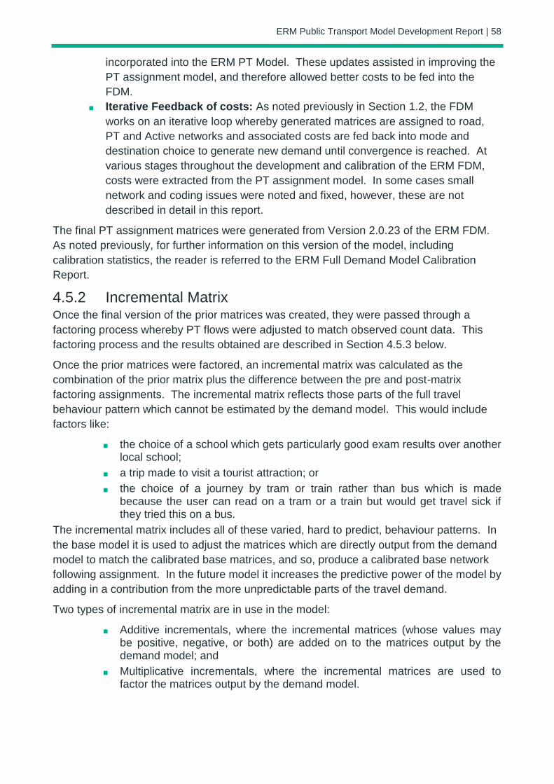
ERM Public Transport Model Development Report | 58
incorporated into the ERM PT Model. These updates assisted in improving the
PT assignment model, and therefore allowed better costs to be fed into the
FDM.
Iterative Feedback of costs: As noted previously in Section 1.2, the FDM
works on an iterative loop whereby generated matrices are assigned to road,
PT and Active networks and associated costs are fed back into mode and
destination choice to generate new demand until convergence is reached. At
various stages throughout the development and calibration of the ERM FDM,
costs were extracted from the PT assignment model. In some cases small
network and coding issues were noted and fixed, however, these are not
described in detail in this report.
The final PT assignment matrices were generated from Version 2.0.23 of the ERM FDM.
As noted previously, for further information on this version of the model, including
calibration statistics, the reader is referred to the ERM Full Demand Model Calibration
Report.
4.5.2 Incremental Matrix Once the final version of the prior matrices was created, they were passed through a
factoring process whereby PT flows were adjusted to match observed count data. This
factoring process and the results obtained are described in Section 4.5.3 below.
Once the prior matrices were factored, an incremental matrix was calculated as the
combination of the prior matrix plus the difference between the pre and post-matrix
factoring assignments. The incremental matrix reflects those parts of the full travel
behaviour pattern which cannot be estimated by the demand model. This would include
factors like:
the choice of a school which gets particularly good exam results over another local school;
a trip made to visit a tourist attraction; or
the choice of a journey by tram or train rather than bus which is made because the user can read on a tram or a train but would get travel sick if they tried this on a bus.
The incremental matrix includes all of these varied, hard to predict, behaviour patterns. In
the base model it is used to adjust the matrices which are directly output from the demand
model to match the calibrated base matrices, and so, produce a calibrated base network
following assignment. In the future model it increases the predictive power of the model by
adding in a contribution from the more unpredictable parts of the travel demand.
Two types of incremental matrix are in use in the model:
Additive incrementals, where the incremental matrices (whose values may be positive, negative, or both) are added on to the matrices output by the demand model; and
Multiplicative incrementals, where the incremental matrices are used to factor the matrices output by the demand model.
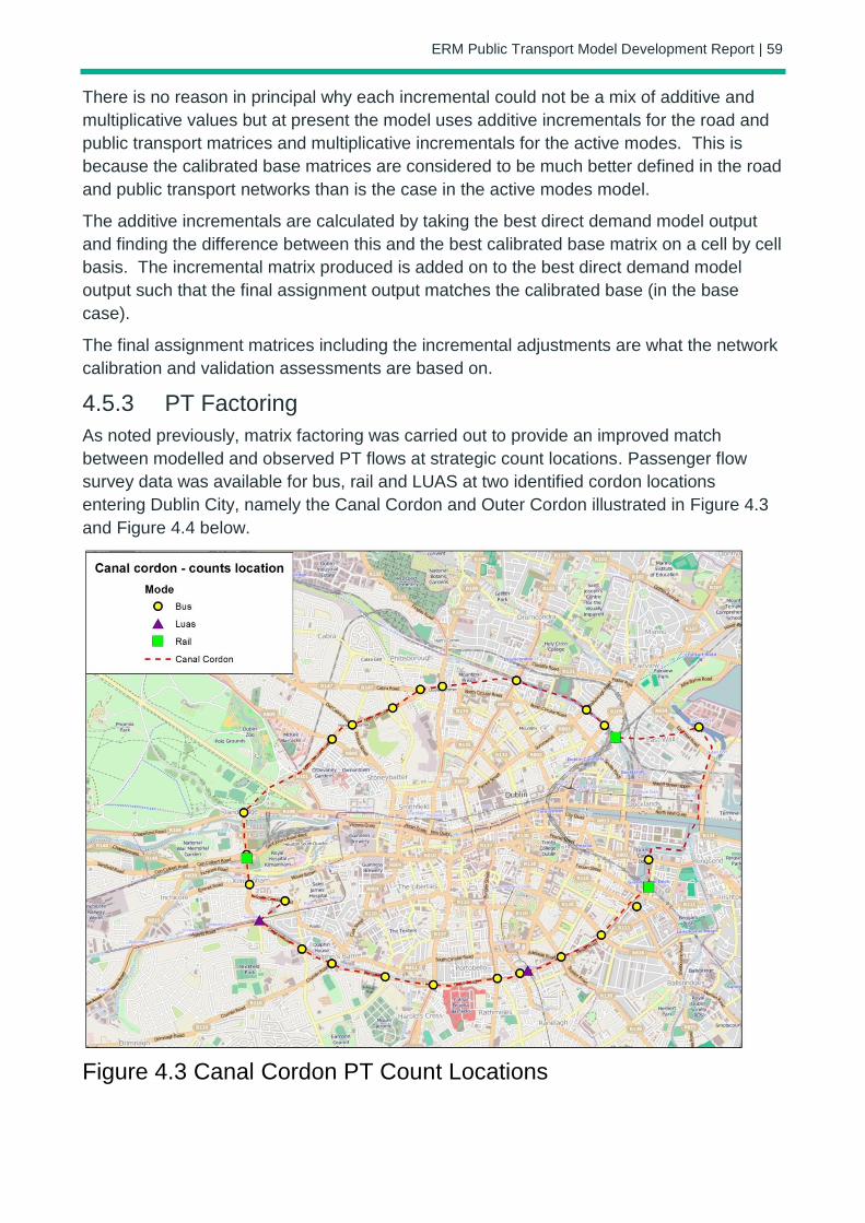
ERM Public Transport Model Development Report | 59
There is no reason in principal why each incremental could not be a mix of additive and
multiplicative values but at present the model uses additive incrementals for the road and
public transport matrices and multiplicative incrementals for the active modes. This is
because the calibrated base matrices are considered to be much better defined in the road
and public transport networks than is the case in the active modes model.
The additive incrementals are calculated by taking the best direct demand model output
and finding the difference between this and the best calibrated base matrix on a cell by cell
basis. The incremental matrix produced is added on to the best direct demand model
output such that the final assignment output matches the calibrated base (in the base
case).
The final assignment matrices including the incremental adjustments are what the network
calibration and validation assessments are based on.
4.5.3 PT Factoring
As noted previously, matrix factoring was carried out to provide an improved match
between modelled and observed PT flows at strategic count locations. Passenger flow
survey data was available for bus, rail and LUAS at two identified cordon locations
entering Dublin City, namely the Canal Cordon and Outer Cordon illustrated in Figure 4.3
and Figure 4.4 below.
Figure 4.3 Canal Cordon PT Count Locations

ERM Public Transport Model Development Report | 60
Figure 4.4 Outer Cordon PT Count Locations
Counts along the identified cordons were grouped into screenlines where observed flows
were combined in an inbound and outbound direction. Figure 4.5, overleaf, illustrates the
six screenlines created at the canal cordon based on the direction entering the city centre.
Select Link analysis was carried out on the assigned PT demand to identify modelled
passenger flows crossing the various screenline locations.
A bespoke spreadsheet tool was used to calculate adjustment factors which could be
applied to the modelled PT demand to provide a better estimate of passenger flows at a
screenline level. These adjustment factors were applied to the ERM PT demand based on
a defined sector system which facilitated control over sub-mode choice (Figure 4.6
overleaf). Through Select Link Analysis, it is possible to identify the origin and destination
for services that travel via a particular count location. The spreadsheet tool utilised this
analysis to apply specific factors to sector to sector movements to better replicate
observed flows.
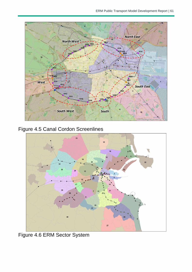
ERM Public Transport Model Development Report | 61
Figure 4.5 Canal Cordon Screenlines
Figure 4.6 ERM Sector System
South East
South
West
South West
North West
North East
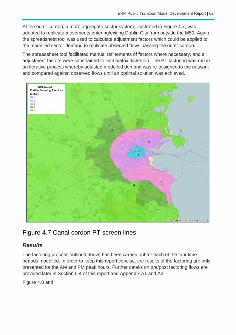
ERM Public Transport Model Development Report | 62
At the outer cordon, a more aggregate sector system, illustrated in Figure 4.7, was
adopted to replicate movements entering/exiting Dublin City from outside the M50. Again
the spreadsheet tool was used to calculate adjustment factors which could be applied to
the modelled sector demand to replicate observed flows passing the outer cordon.
The spreadsheet tool facilitated manual refinements of factors where necessary, and all
adjustment factors were constrained to limit matrix distortion. The PT factoring was run in
an iterative process whereby adjusted modelled demand was re-assigned to the network
and compared against observed flows until an optimal solution was achieved.
Figure 4.7 Canal cordon PT screen lines
Results
The factoring process outlined above has been carried out for each of the four time
periods modelled. In order to keep this report concise, the results of the factoring are only
presented for the AM and PM peak hours. Further details on pre/post factoring flows are
provided later in Section 5.4 of this report and Appendix A1 and A2.
Figure 4.8 and

ERM Public Transport Model Development Report | 63
Figure 4.9 below illustrate the passenger flows by mode at each of the two cordon
locations (displayed in Figure 4.3 and Figure 4.4 previously) for both the prior and post-
factoring matrix compared against observed data.
0
5,000
10,000
15,000
20,000
25,000
30,000
35,000
40,000
45,000
50,000
Bus Luas Rail Total
Pas
sen
ger
Flo
ws
Canal Inbound (AM)
Observed Prior Post Factoring
0
2,000
4,000
6,000
8,000
10,000
12,000
14,000
16,000
18,000
Bus Luas Rail Total
Pas
sen
ger
Flo
ws
Canal Outbound (AM)
Observed Prior Post Factoring
0
5,000
10,000
15,000
20,000
25,000
30,000
35,000
40,000
Bus Luas Rail Total
Pas
sen
ger
Flo
ws
Outer Inbound (AM)
Observed Prior Post Factoring
0
2,000
4,000
6,000
8,000
10,000
12,000
Bus Luas Rail Total
Pas
sen
ger
Flo
ws
Outer Outbound (AM)
Observed Prior Post Factoring

ERM Public Transport Model Development Report | 64
Figure 4.8 Matrix calibration process – Cordon flows - AM peak
hour

ERM Public Transport Model Development Report | 65
Figure 4.9 Matrix calibration process – Cordon flows - PM peak
hour
As outlined on the charts above, the matrix factoring process has improved validation,
particularly in the AM peak, by providing a better match of observed and modelled flows
than was obtained using the prior matrices.
However, the results show that total boardings in the PM peak remain overestimated.
Whilst further factoring could have been undertaken to better match observed flows,
cognisance was taken of changes to the demand generated from the FDM, with careful
consideration to limit overall matrix distortion. Further results on trip matrix validation post
factoring are presented in Section 5.4 of this report.
4.5.4 Sector to Sector Matrix Changes In the ideal case, the amount of change between the directly output demand matrices and
the factored matrices would be small. A comparison of sector to sector movements before
and after PT matrix factoring is shown in Figure 4.10 and Figure 4.11, overleaf. While
there are some larger differences in individual cells, the overall changes in the trip ends
are approximately 3%.
0
2,000
4,000
6,000
8,000
10,000
12,000
14,000
16,000
18,000
Bus Luas Rail Total
Pas
sen
ger
Flo
ws
Canal Inbound (PM)
Observed Prior Post Factoring
0
5,000
10,000
15,000
20,000
25,000
30,000
35,000
Bus Luas Rail Total
Pas
sen
ger
Flo
ws
Canal Outbound (PM)
Observed Prior Post Factoring
0
2,000
4,000
6,000
8,000
10,000
12,000
Bus Luas Rail Total
Pas
sen
ger
Flo
ws
Outer Inbound (PM)
Observed Prior Post Factoring
0
5,000
10,000
15,000
20,000
25,000
30,000
Bus Luas Rail Total
Pas
sen
ger
Flo
ws
Outer Outbound (PM)
Observed Prior Post Factoring
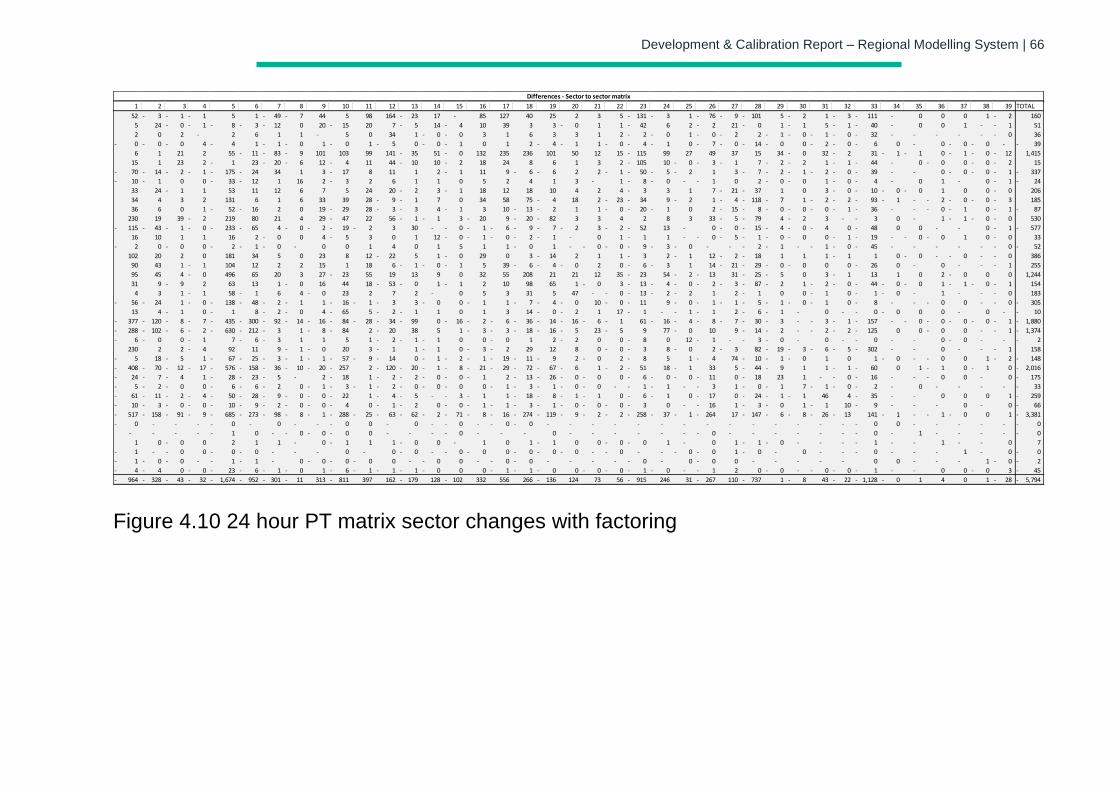
Development & Calibration Report – Regional Modelling System | 66
Figure 4.10 24 hour PT matrix sector changes with factoring
1 2 3 4 5 6 7 8 9 10 11 12 13 14 15 16 17 18 19 20 21 22 23 24 25 26 27 28 29 30 31 32 33 34 35 36 37 38 39 TOTAL
52 3- 1- 1- 5 1 49- 7- 44 5 98 164 23- 17 - 85 127 40 25 2 3 5 131- 3- 1 76- 9- 101- 5 2- 1 3- 111- - 0 0 0 1 2- 160
5 24 0- 1- 8- 3- 12- 0 20 15- 20 7 5- 14 4- 10 39 3 3 0- 1 1 42- 6 2 2- 21 0- 1 1- 5 1- 40- - 0 0 1 - 1- 51
2 0 2 - 2 6 1 1 - 5 0 34 1 0- 0- 3 1 6 3 3 1 2 2- 0- 1 0- 2- 2 1- 0- 1- 0- 32- - - - - - 0- 36
0- 0- 0- 4 4- 1 1- 0- 1 0- 1 5- 0 0- 1- 0 1 2 4- 1- 1 0- 4- 1- 0 7- 0- 14- 0- 0 2- 0- 6- 0 - 0 0- 0- - 39-
6 1 21 2 55 11- 83- 9- 101 103 99 141 35- 51 0- 132 235 236 101 50 12 15 115- 99 27 49 37 15 34 0- 32 2- 31 1- 1- 0 1- 0- 12- 1,415
15 1 23 2 1- 23 20- 6- 12 4- 11 44 10- 10 2- 18 24 8 6 1 3 2 105- 10 0- 3- 1- 7 2- 2- 1 1- 44- - 0 0- 0 0- 2- 15
70- 14- 2- 1- 175- 24- 34 1 3 17- 8 11 1 2 1- 11 9 6- 6- 2 2 1- 50- 5- 2- 1 3 7- 2- 1- 2- 0- 39- - - 0 0- 0- 1- 337-
10- 1- 0 0 33- 12- 1 16 2 3- 2 6 1 1 0 5 2 4 1 3 - 1 8- 0- - 1- 0 2 0- 0- 1 0- 4- - 0 1 - 0 1- 24-
33 24 1- 1 53 11 12 6 7 5 24 20 2- 3 1- 18 12 18 10 4 2 4 3- 3 1 7 21- 37- 1 0 3 0- 10- 0- 0- 1 0 0 0- 206
34 4 3 2 131 6 1 6 33 39 28 9- 1- 7 0 34 58 75 4- 18 2 23- 34- 9 2- 1 4- 118- 7- 1 2- 2- 93- 1- - 2- 0- 0- 3- 185
36 6 0 1 52- 16- 2 0 19 29- 28 3- 3- 4 1- 3 10 13- 2- 1 1 0- 20- 1- 0 2 15- 8- 0- 0- 0- 1- 36- - - 0- 1- 0 1- 87-
230 19 39 2- 219 80 21 4 29 47- 22 56 1- 1- 3 20- 9 20- 82- 3 3 4 2 8 3 33 5- 79- 4 2- 3 - 3- 0 - 1 1- 0- 0- 530
115- 43- 1- 0- 233- 65- 4 0- 2- 19- 2- 3 30 - 0- 1- 6- 9- 7- 2- 3 2- 52- 13 - 0 0- 15- 4- 0- 4- 0 48- 0 0 - - 0 1- 577-
16 10 1 1 16 2 0- 0 4 5- 3 0 1 12 0- 1- 0- 2- 1- - 0 1 1- 1 - 0- 5- 1- 0- 0- 0 1- 19- - 0- 0- 1 0 0- 33
2- 0 0- 0 2- 1- 0- - 0 0 1 4 0 1 5 1 1 0- 1 - 0- 0- 9- 3- 0- - - 2- 1- - 1- 0- 45- - - - - - 0- 52-
102 20 2 0 181 34 5 0 23 8 12 22- 5 1 0- 29 0 3 14- 2 1 1 3- 2 1- 12 2- 18- 1 1 1 1- 1 0 0- - 0- - 0- 386
90 43 1 1- 104 12 2 2 15 1 18 6 1- 0- 1- 5 39 6- 4- 0- 2 0 6- 3- 1 14 21- 29- 0- 0- 0 0 26- 0 - 0 - - 1- 255
95 45 4 0- 496 65 20 3 27 23- 55 19 13 9 0 32 55 208 21 21 12 35 23- 54 2- 13- 31 25- 5- 0 3 1- 13 1 0 2 0- 0 0 1,244
31 9 9- 2 63 13 1 0- 16 44 18 53- 0- 1 1- 2 10 98 65 1 0- 3 13- 4- 0- 2- 3- 87- 2- 1 2- 0- 44- 0- 0- 1 1- 0- 1- 154
4 3 1 1- 58 1- 6 4 0- 23 2 7 2 - 0 5 3 31 5 47 - 0- 13- 2- 2- 1 2 1- 0 0 1- 0 1- 0- - 1 - - 0- 183
56- 24- 1 0- 138- 48- 2- 1- 1 16- 1- 3- 3 0- 0 1- 1 7- 4- 0- 10 0- 11- 9 0- 1- 1- 5- 1- 0- 1- 0 8- - - 0- 0 - 0- 305-
13 4 1- 0 1- 8 2- 0- 4 65- 5 2- 1- 1 0 1 3 14 0- 2- 1 17 1- - 1- 1- 2 6- 1- - 0 - 0- 0- 0 0 - 0 - 10-
377- 120- 8- 7- 435- 300- 92- 14- 16- 84- 28- 34- 99- 0 16- 2- 6- 36- 14- 16- 6- 1- 61 16- 4- 8- 7- 30- 3- - 3- 1- 157- - 0- 0- 0- 0- 1- 1,880-
288- 102- 6- 2- 630- 212- 3- 1 8- 84- 2 20- 38 5 1 3- 3- 18- 16- 5- 23 5- 9 77 0- 10 9 14- 2- - 2- 2- 125- 0 0 0- 0 - 1- 1,374-
6- 0- 0 1- 7 6- 3- 1 1 5 1 2- 1- 1- 0 0 0- 1 2 2- 0 0 8- 0 12 1- - 3- 0- - 0 - 0- - - 0 0- - - 2-
230 2 2 4- 92 11 9 1- 0- 20 3 1- 1 1- 0 3- 2- 29 12 8 0 0- 3- 8 0- 2 3- 82 19- 3- 6- 5- 302- - - 0 - - 1- 158
5- 18 5- 1 67- 25- 3- 1- 1- 57- 9- 14- 0 1- 2- 1- 19- 11- 9- 2 0- 2 8- 5 1 4- 74 10- 1- 0- 1 0 1 0- - 0- 0 1 2- 148-
408- 70- 12- 17- 576- 158- 36- 10- 20- 257- 2 120- 20- 1- 8- 21- 29- 72- 67- 6- 1 2- 51- 18 1- 33 5 44- 9- 1 1 1- 60- 0 1 1- 0 1- 0 2,016-
24- 7- 4- 1 28- 23- 5- - 2 18- 1 2- 2- 0- 0- 1- 2 13- 26- 0- 0- 0 6- 0- 0- 11- 0 18- 23 1 - 0- 16- - - 0- 0 - 0 175-
5- 2- 0- 0 6- 6- 2- 0 1- 3- 1- 2- 0- 0- 0- 0 1- 3- 1- 0- 0- - 1- 1- - 3- 1 0- 1- 7 1- 0- 2- - 0 - - - - 33-
61- 11- 2- 4- 50- 28- 9- 0- 0- 22- 1 4- 5- - 3- 1- 1 18- 8- 1- 1- 0 6- 1- 0 17- 0 24- 1- 1- 46 4 35- - - 0 0 0 1 259-
10- 3- 0- 0- 10- 9- 2- 0- 0- 4- 0 1- 2- 0 0- 1- 1- 3- 1- 0- 0- 0- 3- 0 - 16- 1 3- 0- 1 1- 10 9- - - - 0 - 0 66-
517- 158- 91- 9- 685- 273- 98- 8- 1- 288- 25- 63- 62- 2- 71- 8- 16- 274- 119- 9- 2- 2- 258- 37- 1- 264- 17 147- 6- 8- 26- 13- 141 1- - 1- 0- 0 1 3,381-
0- - - - 0- - 0 - - 0- 0 - 0 - 0- - 0- 0- - - - - - - - - - - - - - - 0- 0 - - - - - 0-
- - - - 1- 0 - 0- 0- 0- 0 - - - 0- - - - 0 - - - - - - 0- - - - - - - 0- - 1 - - - - 0-
1 0 0- 0 2 1 1 - 0 1- 1 1 0- 0 - 1 0 1 1- 0 0 0- 0- 1 - 0 1 1- 0- - - - 1- - - 1 - - 0 7
1- - 0- 0 0- 0- - - - 0 - 0 0- - 0- 0- 0 0- 0- 0- - 0- - - 0- 0- 1 0- - 0 - - 0- - - - 1 - 0 0-
1- 0- 0- - 1- 1- - 0 0- 0- 0- 0 - 0- 0 - 0- 0- - - - - 0- - 0 0- 0 - - - - - 0 0 - - - 1 0- 2-
4- 4- 0 0- 23- 6- 1- 0- 1 6- 1- 1- 1- 0- 0 0 1- 1- 0- 0 0- 0- 1- 0- - 1- 2 0 0- - 0- 0- 1- - - 0 0 0- 3 45-
964- 328- 43- 32- 1,674- 952- 301- 11- 313 811- 397 162 179- 128 102- 332 556 266 136- 124 73 56 915- 246 31 267- 110 737- 1 8- 43 22- 1,128- 0- 1 4 0 1 28- 5,794-
Differences - Sector to sector matrix
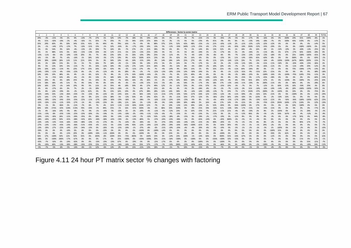
ERM Public Transport Model Development Report | 67
Figure 4.11 24 hour PT matrix sector % changes with factoring
1 2 3 4 5 6 7 8 9 10 11 12 13 14 15 16 17 18 19 20 21 22 23 24 25 26 27 28 29 30 31 32 33 34 35 36 37 38 39 TOTAL
24% -3% -21% -5% 2% 0% -13% -7% 27% 1% 32% 14% -7% 18% 0% 19% 24% 6% 4% 2% 4% 7% -21% -1% 3% -35% -2% -5% 6% -17% 0% -16% -6% 0% 200% 23% 31% 140% -8% 1%
4% 51% -50% -14% -2% -4% -16% 1% 35% -7% 25% 7% -5% 34% -32% 22% 30% 2% 3% -1% 5% 5% -23% 4% 41% -9% 9% 0% 3% -13% 14% -18% -7% 0% 100% 43% 133% 0% -12% 1%
35% 29% 60% 0% 30% 34% 15% 41% 0% 49% 4% 79% 16% -7% -9% 9% 88% 37% 15% 52% 42% 48% -15% -1% 21% -10% -12% 2% -11% -22% -12% -22% -12% 0% 0% 0% 0% 0% -14% 5%
0% -1% -14% 37% -12% 7% -10% -31% 15% -1% 32% -30% 3% -17% -33% 10% 13% 5% -12% -50% 140% -12% -25% -6% 17% -31% -6% -30% -10% 200% -52% -33% -20% 0% 0% 0% -100% -100% 0% -10%
2% 0% 54% 9% 16% -4% -13% -2% 39% 7% 16% 8% -7% 27% -2% 21% 38% 9% 6% 8% 7% 2% -14% 8% 13% 52% 4% 1% 18% -4% 16% -8% 1% -32% -19% 3% -60% -13% -25% 6%
4% 1% 48% 15% 0% 26% -15% -13% 20% -3% 12% 21% -5% 32% -13% 25% 24% 3% 5% 2% 5% 6% -20% 2% -2% -17% 0% 2% -4% -26% 2% -11% -8% 0% 67% -27% 50% -100% -28% 0%
-13% -11% -8% -6% -19% -13% 20% 3% 7% -8% 23% 10% 1% 26% -10% 29% 25% -3% -11% 4% 7% -4% -14% -3% -8% 6% 9% -7% -23% -23% -12% -13% -18% 0% 0% 25% -100% -100% -41% -9%
-6% -5% 8% 7% -6% -16% 1% 18% 14% -3% 17% 19% 9% 42% 100% 41% 23% 6% 5% 42% 0% 16% -6% 0% 0% -15% 3% 11% -14% -50% 45% -60% -8% 0% 0% 300% 0% 0% -83% -2%
14% 30% -100% 26% 11% 11% 21% 33% 5% 3% 50% 19% -6% 30% -31% 24% 8% 14% 18% 14% 25% 27% -6% 4% 11% 15% -16% -12% 19% 7% 13% -16% -4% -100% -100% 167% 300% 100% -15% 7%
6% 2% 18% 15% 8% 5% 1% 7% 26% 7% 18% -2% -1% 19% 9% 19% 37% 5% 0% 10% 5% -7% -17% 5% -3% 2% -2% -14% -12% 19% -4% -31% -11% -50% 0% -20% -40% -25% -36% 2%
9% 5% 13% 19% -6% -11% 7% 3% 33% -12% 34% -9% -12% 17% -14% 21% 26% -8% -3% 14% 8% -4% -28% -2% 10% 10% -6% -7% -3% -17% -3% -26% -11% 0% 0% -11% -29% 29% -12% -3%
14% 10% 63% -11% 9% 23% 17% 15% 24% -6% 42% 9% -2% -11% 17% -8% 7% -4% -24% 9% 34% 15% 1% 9% 32% 21% -4% -11% 64% -26% 8% 0% -1% 0% 0% 73% -100% -17% -14% 6%
-24% -29% -11% -6% -33% -22% 6% -2% -6% -12% -6% 4% 28% 0% -2% -7% -22% -13% -20% -23% 13% -30% -24% 5% 0% 4% -1% -11% -31% -9% -31% 22% -21% 0% 0% 0% 0% 0% -38% -18%
10% 14% 19% 38% 6% 4% -1% 6% 32% -7% 8% 1% 17% 33% -100% -33% -2% -5% -7% 0% 12% 40% -4% 6% 0% -3% -9% -2% -38% -25% 3% -100% -16% 0% -100% -75% 120% 75% -11% 3%
-7% 1% -75% 10% -8% -6% -2% 0% 13% 2% 18% 34% 6% 86% 55% 20% 32% -10% 14% 0% -22% -6% -40% -14% -50% 0% 0% -9% -25% 0% -17% -43% -28% 0% 0% 0% 0% 0% -60% -14%
15% 20% 4% 6% 18% 25% 9% 1% 24% 3% 45% -7% 18% 16% -4% 26% 1% 2% -17% 10% 46% 18% -6% 10% -22% 16% -4% -8% 70% 91% 20% -67% 1% 0% -100% 0% -100% 0% -25% 10%
11% 18% 18% -6% 11% 7% 4% 14% 9% 0% 33% 4% -3% -5% -13% 15% 31% -5% -8% -4% 54% 2% -17% -9% 18% 17% -13% -14% -11% -33% 3% 200% -11% 0% 0% 40% 0% 0% -28% 6%
10% 16% 13% -1% 14% 19% 9% 5% 21% -1% 35% 4% 18% 30% 4% 27% 49% 12% 1% 12% 53% 9% -15% 37% -5% -15% 19% -3% -7% 3% 7% -12% 1% 60% 13% 16% -50% 29% 3% 8%
4% 6% -27% 6% 3% 7% 2% -1% 28% 3% 31% -18% -1% 7% -8% 2% 25% 6% 4% 4% -3% 2% -28% -8% -3% -2% -7% -12% -3% 31% -16% -16% -10% -14% -8% 20% -100% -100% -50% 1%
2% 8% 14% -29% 6% -2% 12% 62% 0% 9% 15% 16% 19% 0% 67% 38% 28% 15% 14% 58% 0% -14% -14% -18% -13% 7% 19% -7% 17% 150% -37% 200% -3% -100% 0% 33% 0% 0% -75% 8%
-42% -44% 33% -13% -46% -43% -5% -15% 8% -23% -6% -24% 10% -4% 36% -34% 11% -21% -37% -10% 54% -67% -50% 12% -33% -12% -4% -11% -69% -4% -42% 33% -21% 0% 0% -100% 0% 0% -14% -29%
12% 14% -17% 13% 0% 14% -6% -8% 22% -15% 38% -5% -13% 50% 4% 19% 42% 3% 0% -21% 33% 37% -12% 0% -36% -25% 30% -19% -50% 0% 133% 0% -2% -33% 33% 5% 0% 0% 0% 0%
-40% -39% -33% -34% -35% -35% -22% -11% -27% -28% -30% -19% -36% 1% -38% -5% -16% -21% -25% -16% -23% -9% 8% -5% -6% -40% -15% -17% -28% 0% -19% -61% -21% 0% -50% -36% -100% -100% -62% -25%
-32% -33% -22% -11% -35% -27% -1% 4% -10% -25% 3% -18% 11% 16% 2% -13% -8% -9% -24% -28% 30% -48% 2% 16% -4% 17% 14% -5% -21% 0% -9% -75% -25% 200% 100% -27% 133% 0% -22% -19%
-9% -1% 9% -86% 2% -21% -7% 6% 7% 4% 31% -11% -21% -83% 150% 12% -7% 1% 19% -13% 13% 20% -10% 2% 52% -83% 0% -56% -100% 0% 17% 0% -5% 0% 0% 33% -100% 0% 0% 0%
40% 10% 275% -32% 124% 114% 70% -24% -1% 49% 25% -1% 16% -31% 100% -4% -4% 86% 33% 104% 4% -8% -25% 19% -16% 51% -10% 10% -17% -15% -5% -14% -15% 0% 0% 0% 0% 0% -77% 4%
-1% 4% -16% 14% -4% -8% -7% -9% -1% -14% -3% -10% 1% -2% -20% -3% -11% -5% -12% 23% -1% 32% -15% 7% 21% -11% 21% -4% -8% -33% 2% 8% 1% -100% 0% -6% 1% 28% -3% -2%
-15% -13% -8% -25% -13% -25% -23% -30% -5% -19% 1% -14% -10% -2% -19% -11% -12% -6% -7% -23% 1% -4% -23% 5% -15% 3% 2% -1% -12% 46% 0% -5% -2% 50% 167% -6% 4% -52% 2% -9%
-20% -15% -30% 26% -11% -26% -35% 0% 28% -20% 9% -19% -13% -13% -7% -32% 53% -12% -28% -8% -15% 3% -39% -2% -17% -19% 3% -12% 8% 9% 0% 0% -3% 0% 0% -17% 50% 0% 44% -8%
-28% -20% -20% 50% -31% -38% -42% 20% -30% -38% -22% -19% -4% -13% -80% 5% -37% -34% -23% -38% -3% 0% -65% -24% 0% -20% 300% -3% -5% 1% -4% 0% 0% 0% 0% 0% 0% 0% 0% -3%
-23% -14% -13% -51% -16% -33% -38% -13% -1% -27% 4% -7% -22% 0% -36% -6% 3% -27% -35% -16% -14% 13% -21% -3% 40% -20% 1% -7% -1% -5% 8% 8% -2% 0% 0% 0% 40% 17% 7% -7%
-27% -23% -13% -43% -23% -36% -51% -43% -6% -31% 5% -23% -24% 40% -22% -29% -22% -29% -29% -20% -36% -100% -61% 6% 0% -50% 39% -9% -1% 1% -1% 29% -2% 0% 0% 0% 0% 0% 0% -7%
-23% -20% -27% -22% -19% -32% -34% -13% 0% -26% -6% -15% -20% -1% -37% -8% -6% -21% -19% -20% -4% -4% -30% -6% -9% -19% 5% -5% -1% -2% -1% -3% 1% -100% 0% -5% -2% 6% 3% -10%
-50% 0% 0% 0% -10% 0% 0% 0% 0% -20% 0% 0% 0% 0% -100% 0% -100% -14% 0% 0% 0% 0% 0% 0% 0% 0% 0% 0% 0% 0% 0% 0% -100% 32% 0% 0% 0% 0% 0% 0%
0% 0% 0% 0% -15% 20% 0% -100% -50% -11% 200% 0% 0% 0% -100% 0% 0% 0% 23% 0% 0% 0% 0% 0% 0% -100% 0% 0% 0% 0% 0% 0% -50% 0% 62% 0% 0% 0% 0% -1%
56% 17% -100% 50% 22% 50% 55% 0% 200% -8% 100% 35% -75% 400% 0% 140% 33% 4% -14% 23% 100% -1% -14% 64% 0% 400% 55% -10% -67% 0% 0% 0% -12% 0% 0% 79% 0% 0% 0% 10%
-38% 0% -100% 200% -17% -67% 0% 0% 0% 17% 0% 25% -100% 0% -100% -100% 20% -25% -50% -100% 0% -100% 0% 0% -100% -100% 10% -10% 0% 0% 0% 0% -7% 0% 0% 0% 11% 0% 27% -1%
-45% -7% -50% 0% -24% -83% 0% 0% -33% -29% -23% 67% 0% -29% 0% 0% -25% -17% 0% 0% 0% 0% -100% 0% 0% -100% 7% 0% 0% 0% 0% 0% 4% 0% 0% 0% 0% 55% -21% -7%
-9% -20% 40% -13% -30% -38% -33% -25% 15% -37% -5% -14% -24% -6% 25% 57% -17% -7% -10% 200% -22% -60% -42% -2% 0% -46% 3% 3% -40% 0% -2% -100% -3% 0% 0% 0% 6% -20% 19% -12%
-5% -7% -5% -8% -5% -14% -8% -1% 12% -6% 13% 2% -6% 15% -21% 13% 18% 2% -1% 7% 10% 3% -15% 4% 5% -7% 2% -4% 0% -1% 1% -3% -4% -3% 8% 5% 0% 5% -9% -3%
Differences - Sector to sector matrix

Development & Calibration Report – Regional Modelling System | 68
4.5.5 R² Analysis Regression statistics (Slopes, Intercepts and R² values) have been calculated to monitor
the changes made to the PT matrices during factoring. TAG Unit M3-1, Section 8, Table 5
outlines criteria for each of these statistics at both a zonal cell and trip-end level (Table
4.10).
Table 4.10 Significance of Matrix Estimation Changes
Measure Significance Criteria
Matrix zonal cell value Slope within 0.98 and 1.02;
Intercept near zero;
R2 in excess of 0.95.
Matrix zonal trip ends Slope within 0.99 and 1.01;
Intercept near zero;
R2 in excess of 0.98.
AM Table 4.11 details the AM peak R² statistics at the zonal cell level for each individual PT
User Class.
Table 4.11 AM Matrix Change R2 Analysis – Matrix Zonal Cell
Values
User Class Cell R2 Value Cell Slope Cell Y-Int
TAG Criteria > 0.95 0.98 - 1.02 Near 0
Employers Business 0.402 0.506 0.029
Commute 0.820 0.829 0.015
Other 0.967 0.905 0.002
Education 0.943 0.956 -0.004
Retired 0.311 -0.644 0.100
Only the ‘Other’ user class meets the recommended R² criteria, whilst all five user classes
fail to meet the slope criteria. The slope and R² values fall well outside the acceptable
range for the Employers Business and Retired user classes, however, they only represent
approximately 5% of the overall AM PT demand.
Trip end analysis was also undertaken for each user class and the results are summarised
in Table 4.12.
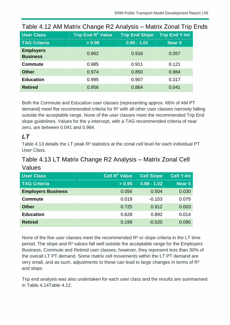
ERM Public Transport Model Development Report | 69
Table 4.12 AM Matrix Change R2 Analysis – Matrix Zonal Trip Ends
User Class Trip End R2 Value Trip End Slope Trip End Y-Int
TAG Criteria > 0.98 0.99 - 1.01 Near 0
Employers
Business 0.962 0.916 0.057
Commute 0.985 0.911 0.121
Other 0.974 0.850 0.984
Education 0.995 0.907 0.317
Retired 0.956 0.864 0.041
Both the Commute and Education user classes (representing approx. 66% of AM PT
demand) meet the recommended criteria for R² with all other user classes narrowly falling
outside the acceptable range. None of the user classes meet the recommended Trip End
slope guidelines. Values for the y-intercept, with a TAG recommended criteria of near
zero, are between 0.041 and 0.984.
LT Table 4.13 details the LT peak R² statistics at the zonal cell level for each individual PT
User Class.
Table 4.13 LT Matrix Change R2 Analysis – Matrix Zonal Cell
Values
User Class Cell R2 Value Cell Slope Cell Y-Int
TAG Criteria > 0.95 0.98 - 1.02 Near 0
Employers Business 0.056 0.504 0.030
Commute 0.019 -0.153 0.075
Other 0.725 0.912 0.003
Education 0.628 0.892 0.014
Retired 0.199 -0.520 0.095
None of the five user classes meet the recommended R² or slope criteria in the LT time
period. The slope and R² values fall well outside the acceptable range for the Employers
Business, Commute and Retired user classes, however, they represent less than 30% of
the overall LT PT demand. Some matrix cell movements within the LT PT demand are
very small, and as such, adjustments to these can lead to large changes in terms of R²
and slope.
Trip end analysis was also undertaken for each user class and the results are summarised
in Table 4.14Table 4.12.

ERM Public Transport Model Development Report | 70
Table 4.14 LT Matrix Change R2 Analysis – Matrix Zonal Trip Ends
User Class Trip End R2 Value Trip End Slope Trip End Y-Int
TAG Criteria > 0.98 0.99 - 1.01 Near 0
Employers
Business 0.871 0.947 0.011
Commute 0.961 0.835 0.108
Other 0.926 0.873 0.567
Education 0.975 1.052 -0.002
Retired 0.962 0.865 0.053
All five user classes narrowly fall outside the acceptable range for both R² and Trip End
Slope. Values for the y-intercept, with a TAG recommended criteria of near zero, are
between -0.002 and 0.567.
SR Table 4.15 details the SR peak R² statistics at the zonal cell level for each individual PT
User Class.
Table 4.15 SR Matrix Change R2 Analysis – Matrix Zonal Cell
Values
User Class Cell R2 Value Cell Slope Cell Y-Int
TAG Criteria > 0.95 0.98 - 1.02 Near 0
Employers Business 0.171 0.474 0.035
Commute 0.090 0.344 0.054
Other 0.757 0.982 0.001
Education 0.771 0.903 0.015
Retired 0.488 -0.868 0.110
None of the five user classes meet the recommended R² in the SR time period. The ‘Other’
user class meets the slope criteria with all other user classes falling outside the acceptable
range. The slope and R² values fall well outside the acceptable range for the Employers
Business, Commute and Retired user classes, however, they represent less than 25% of
the overall SR PT demand. Some matrix cell movements within the SR PT demand are
very small, and as such, adjustments to these can lead to large changes in terms of R²
and slope.
Trip end analysis was also undertaken for each user class and the results are summarised
in Table 4.16Table 4.12.

ERM Public Transport Model Development Report | 71
Table 4.16 SR Matrix Change R2 Analysis – Matrix Zonal Trip Ends
User Class Trip End R2 Value Trip End Slope Trip End Y-Int
TAG Criteria > 0.98 0.99 - 1.01 Near 0
Employers
Business 0.942 1.084 -0.026
Commute 0.986 1.107 -0.098
Other 0.938 1.012 -0.186
Education 0.993 1.055 -0.031
Retired 0.913 0.928 0.007
Both the Commute and Education user classes (representing approx. 41% of SR PT
demand) meet the recommended criteria for R² with all other user classes narrowly falling
outside the acceptable range. None of the user classes meet the recommended Trip End
slope guidelines. Values for the y-intercept, with a TAG recommended criteria of near
zero, are between -0.186 and 0.007.
PM Table 4.17 details the PM peak R² statistics at the zonal cell level for each individual PT
User Class.
Table 4.17 PM Matrix Change R2 Analysis – Matrix Zonal Cell
Values
User Class Cell R2 Value Cell Slope Cell Y-Int
TAG Criteria > 0.95 0.98 - 1.02 Near 0
Employers Business 0.105 0.461 0.031
Commute 0.805 0.854 0.027
Other 0.736 0.921 0.010
Education 0.923 0.984 0.005
Retired 0.375 -0.719 0.101
None of the five user classes meet the recommended R² criteria whilst only the Education
user class meets the slope criteria. The Employers Business and Retired user classes fall
well outside the acceptable range, however, they represent less than 7% of the overall PM
PT demand.
Trip end analysis was also undertaken for each user class and the results are summarised
in Table 4.18.
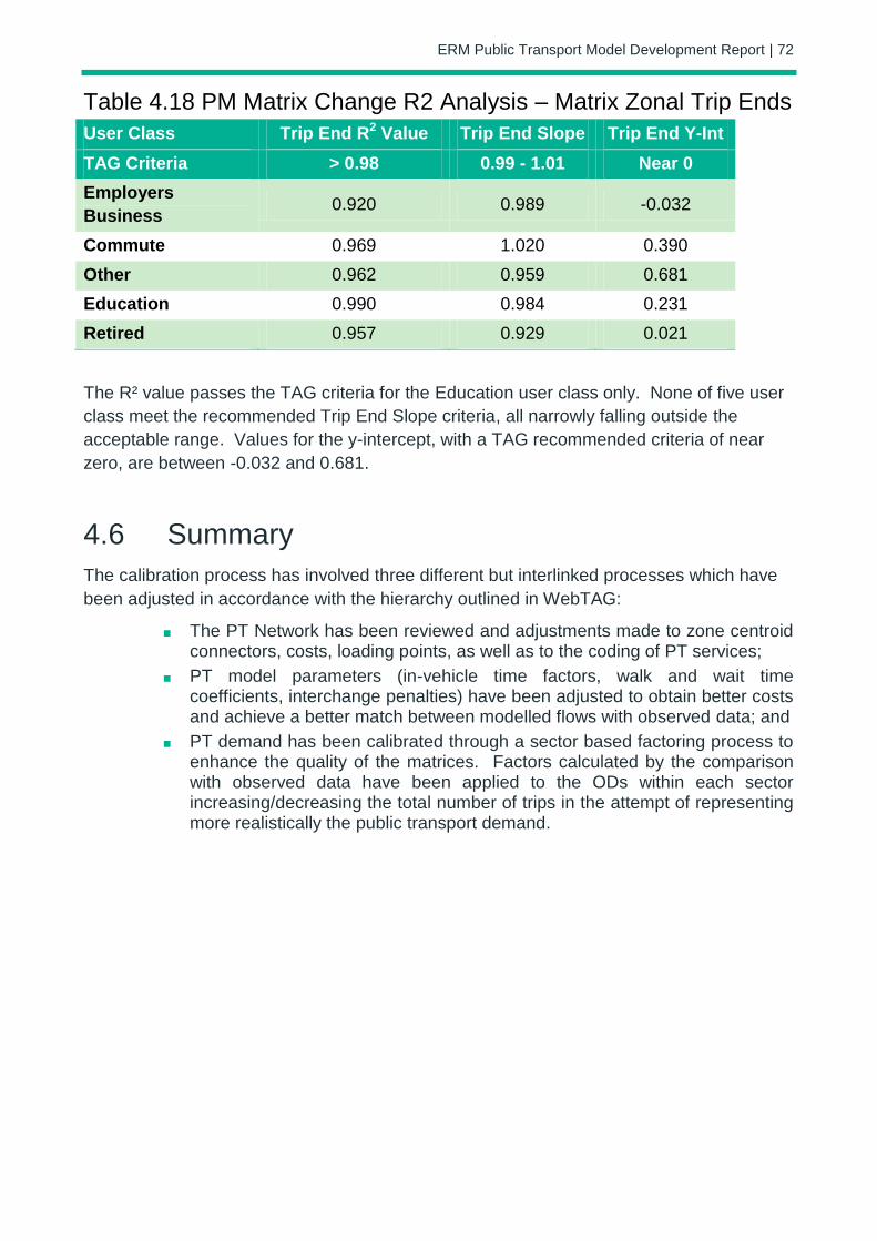
ERM Public Transport Model Development Report | 72
Table 4.18 PM Matrix Change R2 Analysis – Matrix Zonal Trip Ends
User Class Trip End R2 Value Trip End Slope Trip End Y-Int
TAG Criteria > 0.98 0.99 - 1.01 Near 0
Employers
Business 0.920 0.989 -0.032
Commute 0.969 1.020 0.390
Other 0.962 0.959 0.681
Education 0.990 0.984 0.231
Retired 0.957 0.929 0.021
The R² value passes the TAG criteria for the Education user class only. None of five user
class meet the recommended Trip End Slope criteria, all narrowly falling outside the
acceptable range. Values for the y-intercept, with a TAG recommended criteria of near
zero, are between -0.032 and 0.681.
4.6 Summary
The calibration process has involved three different but interlinked processes which have
been adjusted in accordance with the hierarchy outlined in WebTAG:
The PT Network has been reviewed and adjustments made to zone centroid connectors, costs, loading points, as well as to the coding of PT services;
PT model parameters (in-vehicle time factors, walk and wait time coefficients, interchange penalties) have been adjusted to obtain better costs and achieve a better match between modelled flows with observed data; and
PT demand has been calibrated through a sector based factoring process to enhance the quality of the matrices. Factors calculated by the comparison with observed data have been applied to the ODs within each sector increasing/decreasing the total number of trips in the attempt of representing more realistically the public transport demand.
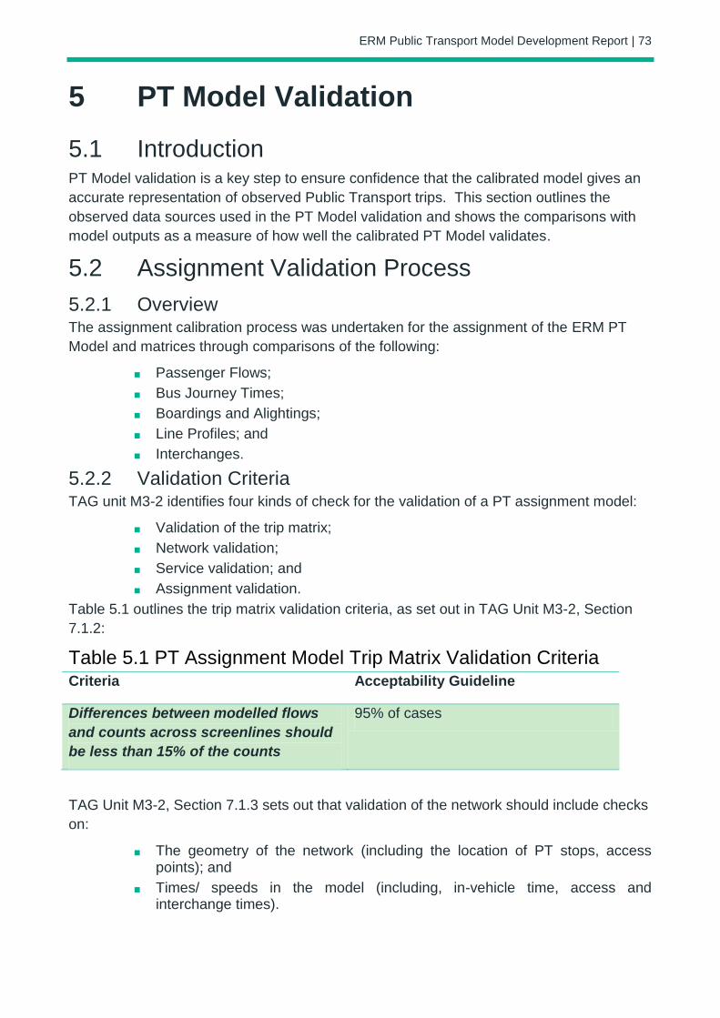
ERM Public Transport Model Development Report | 73
5 PT Model Validation
5.1 Introduction PT Model validation is a key step to ensure confidence that the calibrated model gives an
accurate representation of observed Public Transport trips. This section outlines the
observed data sources used in the PT Model validation and shows the comparisons with
model outputs as a measure of how well the calibrated PT Model validates.
5.2 Assignment Validation Process
5.2.1 Overview The assignment calibration process was undertaken for the assignment of the ERM PT
Model and matrices through comparisons of the following:
Passenger Flows;
Bus Journey Times;
Boardings and Alightings;
Line Profiles; and
Interchanges.
5.2.2 Validation Criteria TAG unit M3-2 identifies four kinds of check for the validation of a PT assignment model:
Validation of the trip matrix;
Network validation;
Service validation; and
Assignment validation.
Table 5.1 outlines the trip matrix validation criteria, as set out in TAG Unit M3-2, Section
7.1.2:
Table 5.1 PT Assignment Model Trip Matrix Validation Criteria Criteria Acceptability Guideline
Differences between modelled flows
and counts across screenlines should
be less than 15% of the counts
95% of cases
TAG Unit M3-2, Section 7.1.3 sets out that validation of the network should include checks
on:
The geometry of the network (including the location of PT stops, access points); and
Times/ speeds in the model (including, in-vehicle time, access and interchange times).
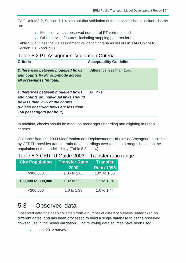
ERM Public Transport Model Development Report | 74
TAG Unit M3-2, Section 7.1.4 sets out that validation of the services should include checks
on:
Modelled versus observed number of PT vehicles; and
Other service features, including stopping patterns for rail.
Table 5.2 outlines the PT assignment validation criteria as set out in TAG Unit M3-2,
Section 7.1.5 and 7.1.6:
Table 5.2 PT Assignment Validation Criteria Criteria Acceptability Guideline
Differences between modelled flows
and counts by PT sub-mode across
all screenlines (in total)
Difference less than 15%
Differences between modelled flows
and counts on individual links should
be less than 25% of the counts
(unless observed flows are less than
150 passengers per hour)
All links
In addition, checks should be made on passengers boarding and alighting in urban
centres.
Guidance from the 2003 Modélisation des Déplacements Urbains de Voyageurs published
by CERTU provides transfer ratio (total boardings over total trips) ranges based on the
population of the modelled city (Table 5.3 below):
Table 5.3 CERTU Guide 2003 – Transfer ratio range
City Population Transfer Ratio
2000
Transfer
Ratio 1995
>300,000 1.05 to 1.65 1.05 to 1.55
100,000 to 300,000 1.02 to 1.33 1.1 to 1.34
<100,000 1.0 to 1.33 1.0 to 1.44
5.3 Observed data Observed data has been collected from a number of different surveys undertaken on
different dates, and has been processed to build a single database to define observed
flows to use in the model validation. The following data sources have been used:
Luas: 2012 survey

ERM Public Transport Model Development Report | 75
Rail: Irish Rail 2013 survey
Bus: different sources (see Table 5.4 below)
Table 5.4 Bus observed flows data sources Screen line Time
Period
Data source Comments
Dublin Bus Other Bus
Canal
Inbound
AM Dublin Bus
survey 2011
Dublin Bus
survey 2011
2014 DublinBus survey
doesn't include private bus
Canal
Inbound
LT / SR Dublin Bus
survey 2014
NDC survey
2015
Canal
Inbound
PM NDC survey
2015 (partial)
NDC survey
2015
Missing counts synthetized
Canal
Outbound
AM Dublin Bus
survey 2011
Dublin Bus
survey 2011
2014 DublinBus survey
doesn't include private bus
Canal
Outbound
LT /SR Dublin Bus
survey 2014
NDC survey
2015
Canal
Outbound
PM Dublin Bus
survey 2014
NDC survey
2015
Outer
Inbound
AM Dublin Bus
survey 2011
Dublin Bus
survey 2011
2014 NDC outer counts 40%
higher than 2011 counts
Outer
Inbound
LT / SR NDC survey
2014
NDC survey
2014
Outer
Inbound
PM NDC survey
2014
NDC survey
2014
Outer
Outbound
AM Dublin Bus
survey 2011
Dublin Bus
survey 2011
2014 NDC outer counts 40%
higher than 2011 counts
Outer
Outbound
LT/SR NDC survey
2014
NDC survey
2014
Outer
Outbound
PM NDC survey
2014
NDC survey
2014

ERM Public Transport Model Development Report | 76
5.4 PT Trip Matrix Validation Table 5.5 below summarises at the screenline level observed flows, modelled flows before
factoring and modelled flows after the factoring process, by time period (further information
on the factoring methodology is provided in Section 4.5.3 previously). More details on
flows by sub-mode and by location are available in Appendix A1 and A2.
The results in Table 5.5 indicate that, with the exception of the SR and PM Outer cordons,
all screenline flows are within +/- 15% observed flows validation criterion.

ERM Public Transport Model Development Report | 77
Table 5.5 Passenger flow validation summary table Time
Period
Cordon Observed Before Factoring After Factoring
Modelled Diff. %Diff. Modelled Diff. %Diff.
AM Canal
Inbound 40,671 46,424 +5,753 +14% 40,264 -407 -1%
AM Canal
Outbound 13,189 16,535 +3,346 +25% 13,973 +784 +6%
AM Outer
Inbound 28,169 36,713 +8,544 +30% 31,751 +3,582 +13%
AM Outer
Outbound 8,357 9,601 +1,244 +15% 8,458 +101 +1%
LT Canal
Inbound 12,110 12,128 +18 +0% 11,158 -952 -8%
LT Canal
Outbound 6,586 7,734 +1,148 +17% 6,457 -129 -2%
LT Outer
Inbound 8,070 9,304 +1,234 +15% 7,684 -386 -5%
LT Outer
Outbound 4,572 5,464 +892 +20% 4,509 -63 -1%
SR Canal
Inbound 10,083 11,442 +1,359 +13% 11,116 +1,033 +10%
SR Canal
Outbound 11,635 12,035 +400 +3% 12,872 +1,237 +11%
SR Outer
Inbound 5,059 7,938 +2,879 +57% 6,466 +1,407 +28%
SR Outer
Outbound 7,370 9,474 +2,104 +29% 9,574 +2,204 +30%
PM Canal
Inbound 15,251 16,300 +1,049 +7% 16,469 +1,218 +8%
PM Canal
Outbound 31,520 31,455 -65 -0% 32,633 +1,113 +4%
PM Outer
Inbound 7,178 10,350 +3,172 +44% 9,723 +2,545 +35%
PM Outer
Outbound 17,542 23,937 +6,395 +36% 23,859 +6,317 +36%
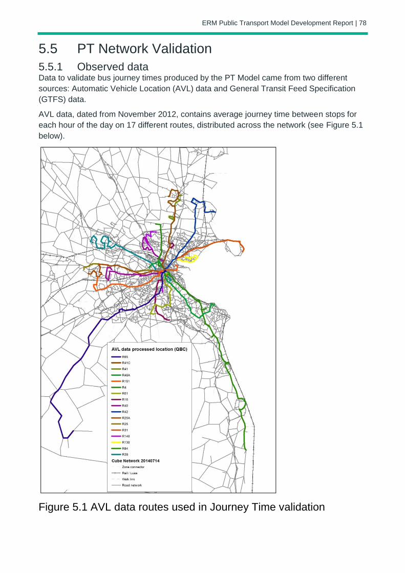
ERM Public Transport Model Development Report | 78
5.5 PT Network Validation
5.5.1 Observed data Data to validate bus journey times produced by the PT Model came from two different
sources: Automatic Vehicle Location (AVL) data and General Transit Feed Specification
(GTFS) data.
AVL data, dated from November 2012, contains average journey time between stops for
each hour of the day on 17 different routes, distributed across the network (see Figure 5.1
below).
Figure 5.1 AVL data routes used in Journey Time validation

ERM Public Transport Model Development Report | 79
As the AVL data has only been processed for a limited number of bus lines, GTFS
timetables are also used to check other bus lines’ journey times. GTFS timetables are not
observed data but planned journey times for each service.
5.5.2 Model validation – AVL data
A total of 69 services modelled journey times are compared against AVL data. Two
indicators have been extracted, the ratio of services faster/slower than AVL data and the
proportion of services within a relative range of observed journey times.
The first indicator summarised in Table 5.6 below measures the balance between services
modelled too fast and services modelled too slowly. The objective is to have half of the
services on each side of the balance. Results for the ERM model are provided in the table
below, which shows that modelled services are slightly faster than observed data in all
time periods.
Table 5.6 Service classification by journey time comparison to AVL
data and by time period AM LT SR PM
Model faster than
observed AVL data 53 (77%) 48 (70%) 50 (72%) 57 (83%)
Model within +/-10min
of the observed AVL
data
46 (67%) 43 (62%) 41 (59%) 36 (52%)
Model slower than
observed AVL data 16 (23%) 21 (30%) 19 (28%) 12 (17%)
Average Journey
Time difference -17% -17% -16% -20%
The second indicator contains two levels of validation, based on the absolute relative
difference between modelled and observed: less than 15% and less than 25%. Table 5.7
provides a summary of these figures for the four time periods.
The results indicate that more than 70% of the modelled journey times are within +/- 25%
the observed journey times for the AM, LT and SR time periods with this value dropping to
57% in the PM peak.

ERM Public Transport Model Development Report | 80
Table 5.7 Journey Time validation against AVL data – Summary
table Criteria AM LT SR PM
<15% Bus services 35 28 31 29
% 51% 41% 45% 42%
<25% Bus services 50 48 50 39
% 72% 70% 72% 57%
Total 69 69 69 69
AVL journey time detailed validation tables are available in Appendix B.
The figure below is a scatter plot that represents modelled and AVL observed data for the
69 services across the four time periods. It shows a good spread of services on each side
of the line y=x which means a good balance between services modelled too slow and
services modelled too fast.
Figure 5.2 Bus times scatter plot – AVL Data
0
20
40
60
80
100
120
140
160
0 40 80 120 160
Mo
de
lled
JT
Timetable JT
All Time PeriodsJourney Time - Modelled VS AVL
AM
LT
SR
PM
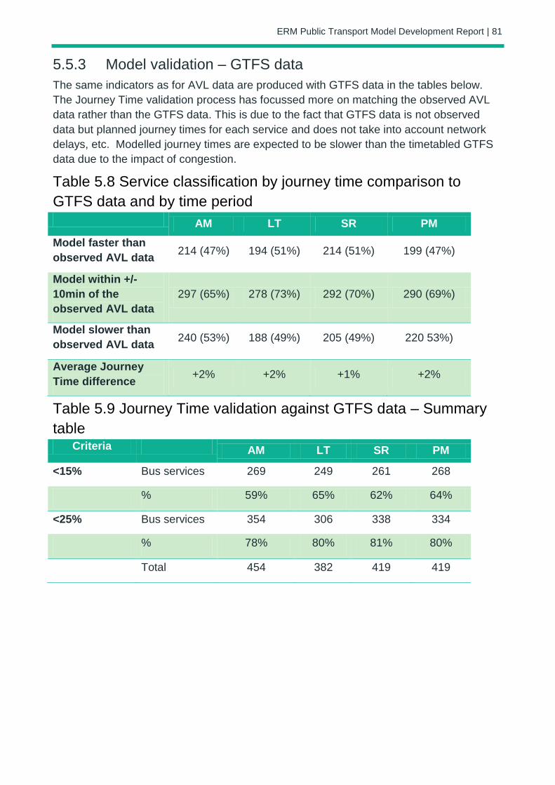
ERM Public Transport Model Development Report | 81
5.5.3 Model validation – GTFS data
The same indicators as for AVL data are produced with GTFS data in the tables below.
The Journey Time validation process has focussed more on matching the observed AVL
data rather than the GTFS data. This is due to the fact that GTFS data is not observed
data but planned journey times for each service and does not take into account network
delays, etc. Modelled journey times are expected to be slower than the timetabled GTFS
data due to the impact of congestion.
Table 5.8 Service classification by journey time comparison to
GTFS data and by time period AM LT SR PM
Model faster than
observed AVL data 214 (47%) 194 (51%) 214 (51%) 199 (47%)
Model within +/-
10min of the
observed AVL data
297 (65%) 278 (73%) 292 (70%) 290 (69%)
Model slower than
observed AVL data 240 (53%) 188 (49%) 205 (49%) 220 53%)
Average Journey
Time difference +2% +2% +1% +2%
Table 5.9 Journey Time validation against GTFS data – Summary
table Criteria AM LT SR PM
<15% Bus services 269 249 261 268
% 59% 65% 62% 64%
<25% Bus services 354 306 338 334
% 78% 80% 81% 80%
Total 454 382 419 419
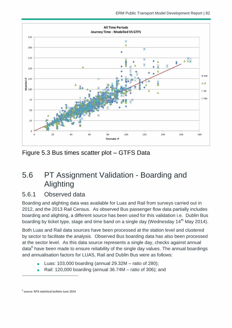
ERM Public Transport Model Development Report | 82
Figure 5.3 Bus times scatter plot – GTFS Data
5.6 PT Assignment Validation - Boarding and Alighting
5.6.1 Observed data
Boarding and alighting data was available for Luas and Rail from surveys carried out in
2012, and the 2013 Rail Census. As observed Bus passenger flow data partially includes
boarding and alighting, a different source has been used for this validation i.e. Dublin Bus
boarding by ticket type, stage and time band on a single day (Wednesday 14th May 2014).
Both Luas and Rail data sources have been processed at the station level and clustered
by sector to facilitate the analysis. Observed Bus boarding data has also been processed
at the sector level. As this data source represents a single day, checks against annual
data6 have been made to ensure reliability of the single day values. The annual boardings
and annualisation factors for LUAS, Rail and Dublin Bus were as follows:
Luas: 103,000 boarding (annual 29.32M – ratio of 280);
Rail: 120,000 boarding (annual 36.74M – ratio of 306); and
6 source: NTA statistical bulletin June 2014
0
25
50
75
100
125
150
175
200
225
0 20 40 60 80 100 120 140 160 180
Mo
de
lled
JT
Timetable JT
All Time PeriodsJourney Time - Modelled VS GTFS
AM
LT
SR
PM
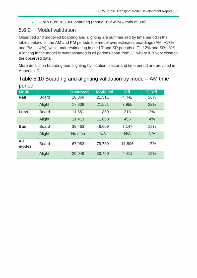
ERM Public Transport Model Development Report | 83
Dublin Bus: 365,000 boarding (annual 112.49M – ratio of 308).
5.6.2 Model validation
Observed and modelled boarding and alighting are summarised by time period in the
tables below. In the AM and PM periods the model overestimates boardings (AM: +17%
and PM: +14%), while underestimating in the LT and SR periods (LT: -12% and SR: -8%).
Alighting in the model is overestimated in all periods apart from LT where it is very close to
the observed data.
More details on boarding and alighting by location, sector and time period are provided in
Appendix C.
Table 5.10 Boarding and alighting validation by mode – AM time
period Mode Observed Modelled Diff. % Diff.
Rail Board 16,869 21,311 4,442 26%
Alight 17,636 21,591 3,955 22%
Luas Board 11,651 11,869 218 2%
Alight 11,413 11,868 456 4%
Bus Board 39,463 46,609 7,147 18%
Alight No data N/A N/A N/A
All
modes Board 67,983 79,789 11,806 17%
Alight 29,049 33,460 4,411 15%
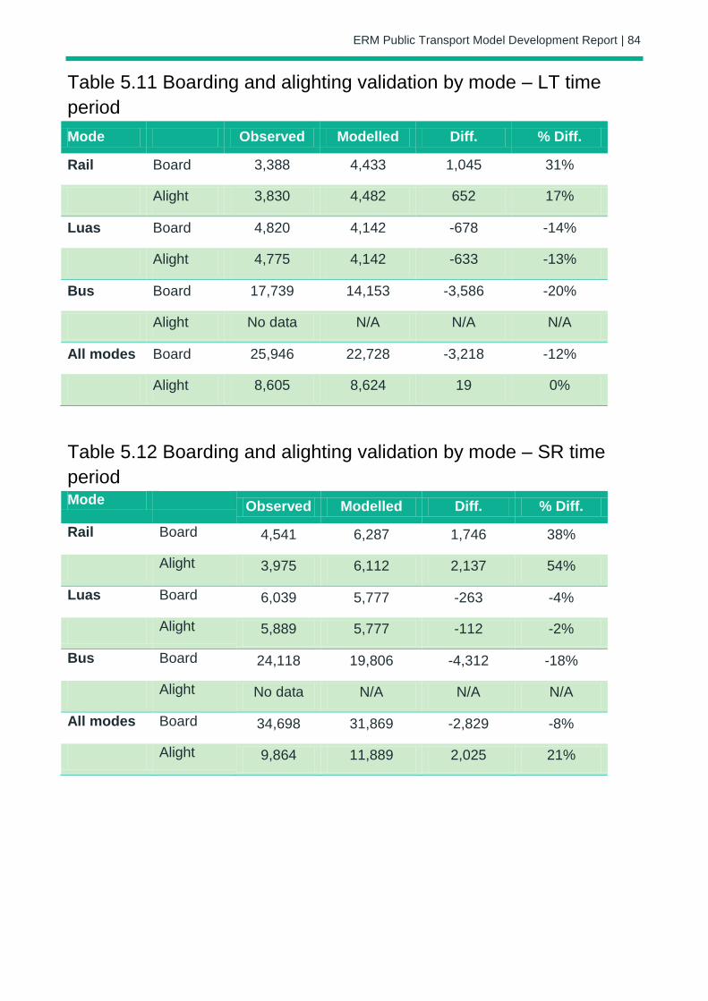
ERM Public Transport Model Development Report | 84
Table 5.11 Boarding and alighting validation by mode – LT time
period
Mode Observed Modelled Diff. % Diff.
Rail Board 3,388 4,433 1,045 31%
Alight 3,830 4,482 652 17%
Luas Board 4,820 4,142 -678 -14%
Alight 4,775 4,142 -633 -13%
Bus Board 17,739 14,153 -3,586 -20%
Alight No data N/A N/A N/A
All modes Board 25,946 22,728 -3,218 -12%
Alight 8,605 8,624 19 0%
Table 5.12 Boarding and alighting validation by mode – SR time
period Mode
Observed Modelled Diff. % Diff.
Rail Board 4,541 6,287 1,746 38%
Alight 3,975 6,112 2,137 54%
Luas Board 6,039 5,777 -263 -4%
Alight 5,889 5,777 -112 -2%
Bus Board 24,118 19,806 -4,312 -18%
Alight No data N/A N/A N/A
All modes Board 34,698 31,869 -2,829 -8%
Alight 9,864 11,889 2,025 21%
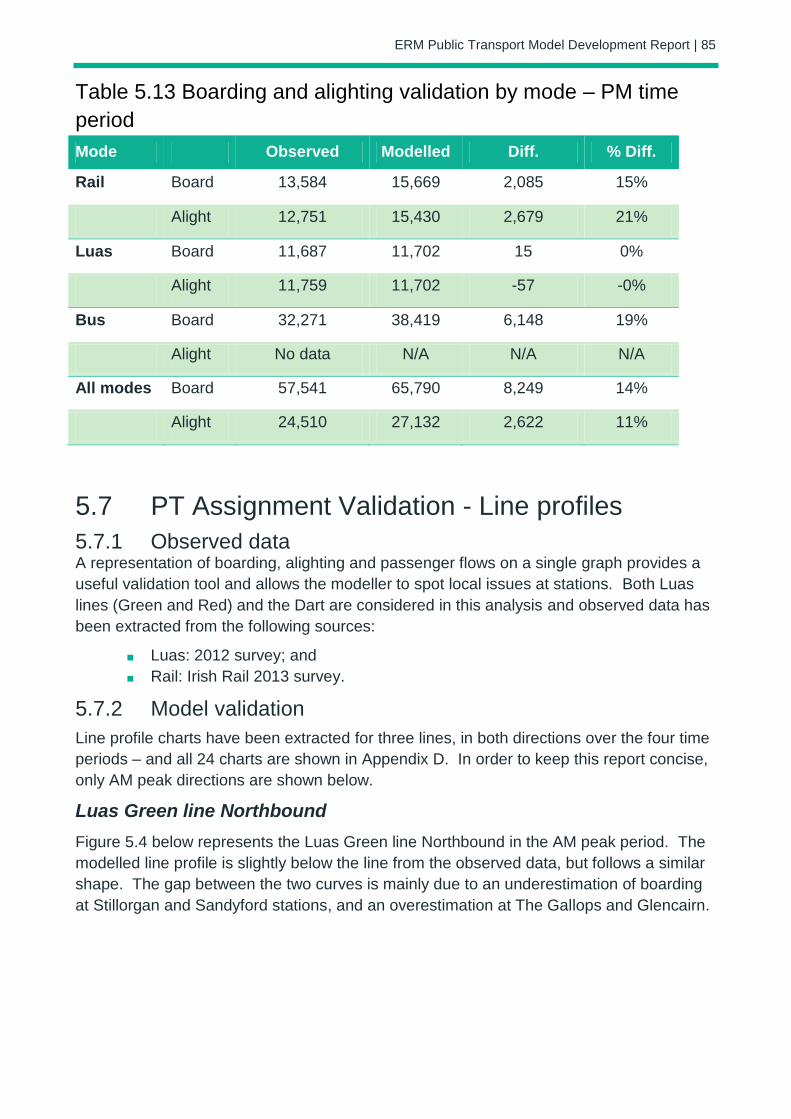
ERM Public Transport Model Development Report | 85
Table 5.13 Boarding and alighting validation by mode – PM time
period
Mode Observed Modelled Diff. % Diff.
Rail Board 13,584 15,669 2,085 15%
Alight 12,751 15,430 2,679 21%
Luas Board 11,687 11,702 15 0%
Alight 11,759 11,702 -57 -0%
Bus Board 32,271 38,419 6,148 19%
Alight No data N/A N/A N/A
All modes Board 57,541 65,790 8,249 14%
Alight 24,510 27,132 2,622 11%
5.7 PT Assignment Validation - Line profiles
5.7.1 Observed data A representation of boarding, alighting and passenger flows on a single graph provides a
useful validation tool and allows the modeller to spot local issues at stations. Both Luas
lines (Green and Red) and the Dart are considered in this analysis and observed data has
been extracted from the following sources:
Luas: 2012 survey; and
Rail: Irish Rail 2013 survey.
5.7.2 Model validation
Line profile charts have been extracted for three lines, in both directions over the four time
periods – and all 24 charts are shown in Appendix D. In order to keep this report concise,
only AM peak directions are shown below.
Luas Green line Northbound
Figure 5.4 below represents the Luas Green line Northbound in the AM peak period. The
modelled line profile is slightly below the line from the observed data, but follows a similar
shape. The gap between the two curves is mainly due to an underestimation of boarding
at Stillorgan and Sandyford stations, and an overestimation at The Gallops and Glencairn.

Development & Calibration Report – Regional Modelling System | 86
Figure 5.4 Luas Green line profile – Northbound – AM peak
0
500
1,000
1,500
2,000
2,500
3,000
3,500
Pas
sen
gers
AM Peak Hr - Luas Green NB
Observed Board Modelled Board Observed Alight Modelled Alight Observed Dep. Load Modelled Dep. Load Modelled Seated Capacity
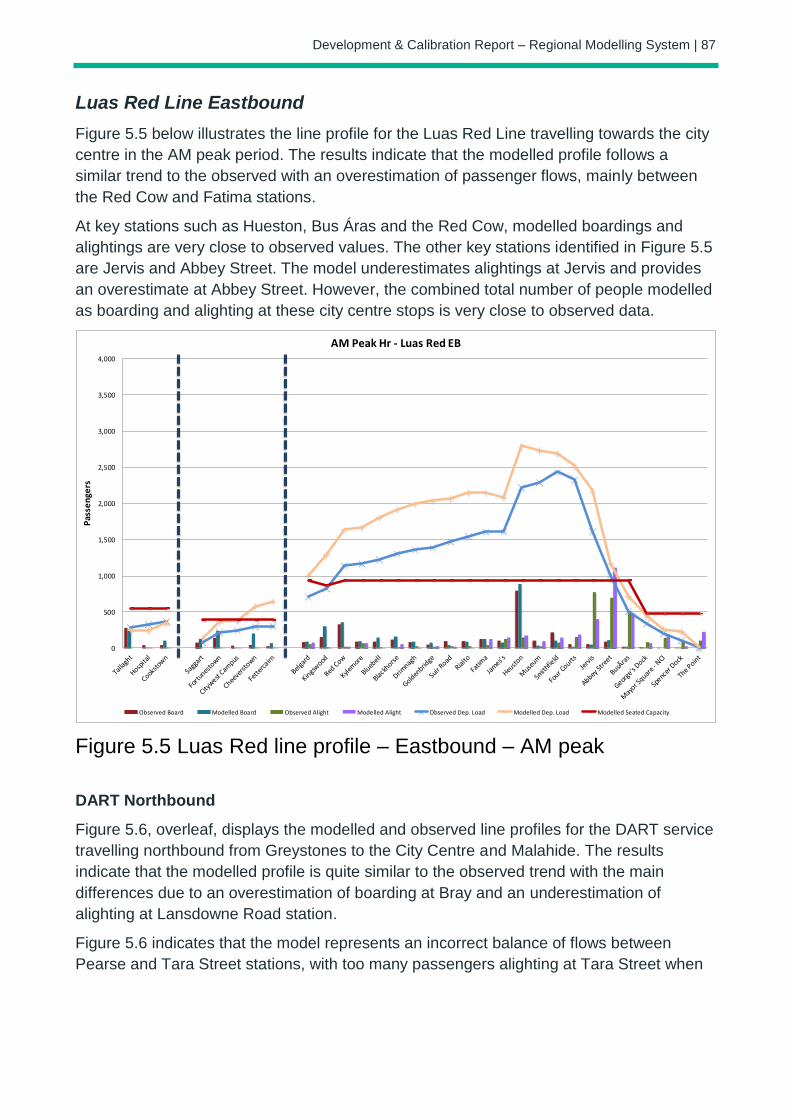
Development & Calibration Report – Regional Modelling System | 87
Luas Red Line Eastbound
Figure 5.5 below illustrates the line profile for the Luas Red Line travelling towards the city
centre in the AM peak period. The results indicate that the modelled profile follows a
similar trend to the observed with an overestimation of passenger flows, mainly between
the Red Cow and Fatima stations.
At key stations such as Hueston, Bus Áras and the Red Cow, modelled boardings and
alightings are very close to observed values. The other key stations identified in Figure 5.5
are Jervis and Abbey Street. The model underestimates alightings at Jervis and provides
an overestimate at Abbey Street. However, the combined total number of people modelled
as boarding and alighting at these city centre stops is very close to observed data.
Figure 5.5 Luas Red line profile – Eastbound – AM peak
DART Northbound
Figure 5.6, overleaf, displays the modelled and observed line profiles for the DART service
travelling northbound from Greystones to the City Centre and Malahide. The results
indicate that the modelled profile is quite similar to the observed trend with the main
differences due to an overestimation of boarding at Bray and an underestimation of
alighting at Lansdowne Road station.
Figure 5.6 indicates that the model represents an incorrect balance of flows between
Pearse and Tara Street stations, with too many passengers alighting at Tara Street when
0
500
1,000
1,500
2,000
2,500
3,000
3,500
4,000
Pas
sen
gers
AM Peak Hr - Luas Red EB
Observed Board Modelled Board Observed Alight Modelled Alight Observed Dep. Load Modelled Dep. Load Modelled Seated Capacity

ERM Public Transport Model Development Report | 88
compared to observed data. However, the combined total number of people modelled as
boarding and alighting at these city centre stops is very close to observed data.
Figure 5.6 DART line profile – Northbound – AM peak
DART Southbound
Figure 5.7 below illustrates the modelled and observed line profiles for the DART service
travelling southbound from Malahide in the AM Peak hour. Similar to the other services,
the modelled line profile follows a similar trend to the observed with peak passenger loads
experienced at Killester and Clontarf Road stations.
The model overestimates passenger demand with approximately 1,500 additional
passengers modelled at Killester station. This is due to an overestimation of passenger
boardings at Kilbarrack, Raheny, Harmonstown and Killester.
The results in Figure 5.7 indicate that the model provides a good representation boarding
and alighting at Connolly station with an incorrect balance of flows at Tara Street and
Pearse Stations i.e. too many passengers alighting at Tara Street and too few at Pearse
when compared to modelled data.
0
500
1,000
1,500
2,000
2,500
3,000
3,500
Pas
sen
gers
AM Peak Hr - Dart NB
Observed Board Modelled Board Observed Alight Modelled Alight Observed Dep. Load Modelled Dep. Load Modelled Seated Capacity
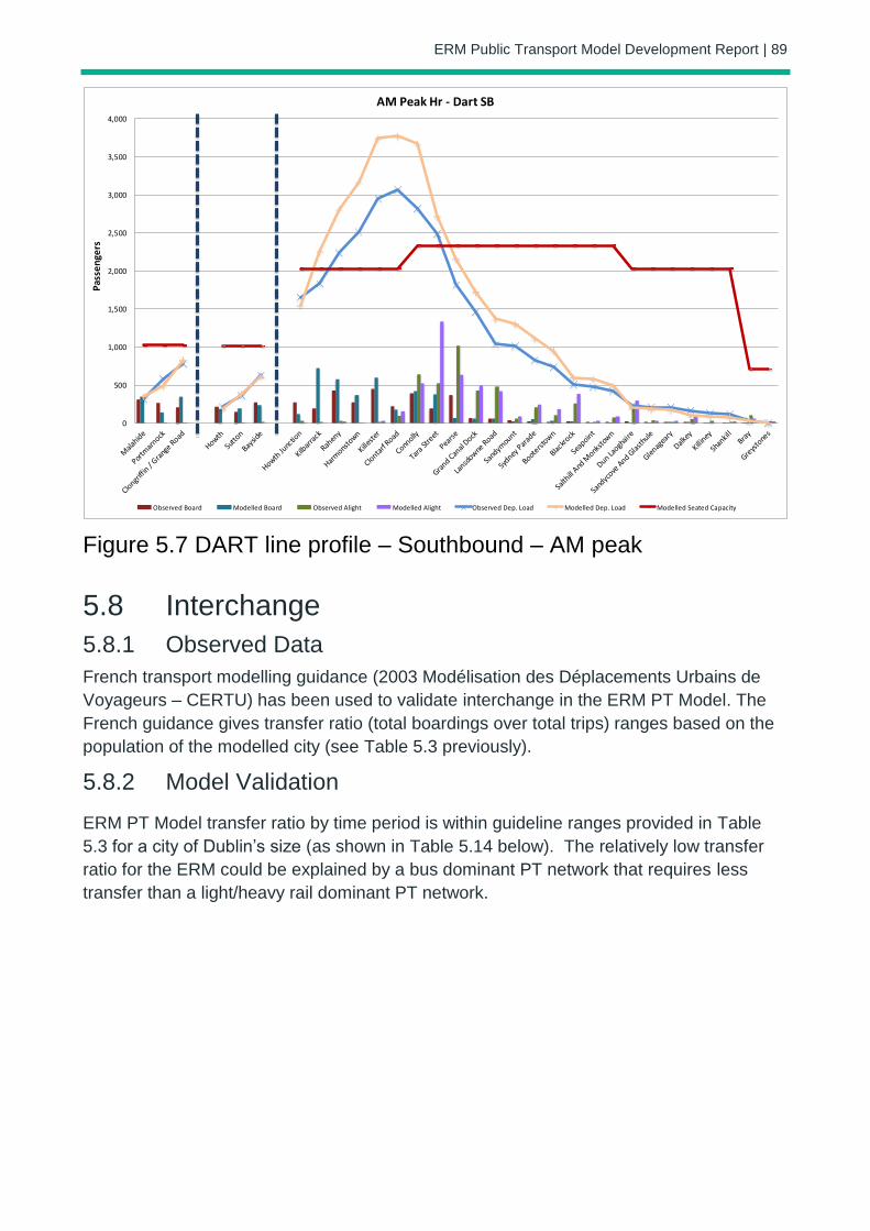
ERM Public Transport Model Development Report | 89
Figure 5.7 DART line profile – Southbound – AM peak
5.8 Interchange
5.8.1 Observed Data
French transport modelling guidance (2003 Modélisation des Déplacements Urbains de
Voyageurs – CERTU) has been used to validate interchange in the ERM PT Model. The
French guidance gives transfer ratio (total boardings over total trips) ranges based on the
population of the modelled city (see Table 5.3 previously).
5.8.2 Model Validation
ERM PT Model transfer ratio by time period is within guideline ranges provided in Table
5.3 for a city of Dublin’s size (as shown in Table 5.14 below). The relatively low transfer
ratio for the ERM could be explained by a bus dominant PT network that requires less
transfer than a light/heavy rail dominant PT network.
0
500
1,000
1,500
2,000
2,500
3,000
3,500
4,000
Pas
sen
gers
AM Peak Hr - Dart SB
Observed Board Modelled Board Observed Alight Modelled Alight Observed Dep. Load Modelled Dep. Load Modelled Seated Capacity

ERM Public Transport Model Development Report | 90
Table 5.14 Overall PT transfer ratio by time period AM LT SR PM
Total Trips 80,778 23,257 33,840 63,505
Intrazonal 4,600 1,567 2,350 1,607
Trips Assigned 76,178 21,690 31,490 61,898
Total Boarding 94,328 28,015 39,093 78,196
Transfer Ratio 1.24 1.29 1.24 1.26
ERM Public Transport Model Development Report | 91
6 Conclusion and Recommendations
6.1 Summary This report has described the development, calibration and validation of the Public
Transport Assignment Model component of the Eastern Regional Model. This section
summarises the key points of the model development, the strength and weakness of the
model revealed by the validation process and a set of recommendations for further
enhancements.
6.2 Model Development – Key points As the PT network is the aggregation of different networks (road, rail, Luas, walking), a
node convention and a link convention have been defined to facilitate output analysis and
provide a framework for any additional network coding.
Bus network speeds are derived from road network congested speed. Factors based on
link characteristics have been calibrated to represent relative bus speed to car speed on
different road types. Bus speeds on bus lanes are defined as car speed on an
uncongested network (or low flow assignment), to take account of traffic light delays.
All PT lines files are automatically derived from General Transit Feed Specification data,
using a bespoke process developed for this model.
Fares are included in the PT assignment model. Separate fare models have been built by
operator, based on ticketing data, to calculate average fare by user class.
6.3 Model Validation Modelled flows for the two cordon screenlines (canal cordon and outer cordon) are within
the acceptance criterion (+/-15%) for the AM period. Canal cordon modelled flows validate
against the acceptance criterion for LT, SR and PM periods. However, the Outer Cordon
flows are overestimated in the SR and PM time periods.
Modelled bus journey time calibration is reasonably good when compared to actual AVL
data with the majority of routes modelled within +/- 10 minutes of observed journey times
with a good balance between services which are too slow and too fast. The results
indicate that more than 70% of the modelled journey times are within +/- 25% of observed
for the AM, LT and SR time periods with this value dropping to 57% in the PM peak
In the AM and PM periods the model overestimates boardings (AM: +17% and PM: +14%),
while underestimating in the LT and SR periods (LT: -12% and SR: -8%). Alighting in the
model is overestimated in all periods apart from LT where it is very close to the observed
data.

ERM Public Transport Model Development Report | 92
Modelled line profiles correspond reasonably well with observed data line profiles. The
main differences between the model and observed data are due to under or over
estimation at a limited number of stations.
The interchange ratio is within the recommended thresholds for a city of Dublin’s size.
6.4 Recommendations Following the development and the calibration/validation of the ERM PT Model, some
areas have been identified where potential improvements could be made.
6.4.1 Analysis of Crowding Cube Voyager software does not allow direct visualisation of crowding. Discussions with
the Citilabs development team are on-going to allow further analysis.
6.4.2 Accessibility for Rural Areas The motorised access mode for PT (mode 96) tends to create long drive access legs. This
can also have an impact on sub-mode choice, particularly in more rural areas of the
model. Re-analysing the motorised access parameters may allow this to be improved.
6.4.3 Additional Surveys Further actions to improve both the calibration and validation processes should be
considered. This could include a more extensive PT survey process to collect more
information on bus, rail and Luas flows at various locations across the entire day and
revenue information to calibrate the fares models.

Development & Calibration Report – Regional Modelling System | 93