forecasting perth’s public transport patronage: … 2016 proceedings 1 forecasting perth’s...

ATRF 2016 Proceedings

1

Forecasting Perth’s public transport patronage: econometric analysis and model

development

Ian Wallis1, Adam Lawrence1

1Ian Wallis Associates, PO Box 11-785, Wellington 6142, New Zealand

Email for correspondence: [email protected]

Abstract

The paper outlines the development and application of a model for forecasting patronage and fare revenues for Perth's public transport services over the medium term. The model development involved the following three main areas of work.

An econometric (time series) analysis was undertaken of Perth's monthly patronage over the last 15 years, using a seasonal difference (‘double-log’) modelling methodology and deriving a set of short run demand elasticities. The model's dependent variable was 'first' boardings (by bus, train) per population per 'standard' month. The main independent variables were average real fare levels, service kilometres, petrol price, employment level and average incomes.

Principally as a check on the elasticity estimates derived for Perth, a review was undertaken of the main econometric studies undertaken in the last 10 years of public transport patronage changes in Australasian metropolitan areas and their resultant elasticity estimates. A surprisingly wide spread of elasticity values was found for each variable in the 10 studies reviewed, although with some signs of estimates clustering around the values expected from wider (international) evidence. In our view, these results indicate not that market responses are very different in different cities; but rather that underlying responses are generally very consistent, and that successful time series modelling is very challenging.

In the light of the above, and based principally on the outputs from the Perth modelling, a 'best estimate' set of elasticity values relevant to Perth was selected. Using these elasticities, a spreadsheet-based forecasting model was formulated, for use by the WA state authorities (principally Transperth/WA Public Transport Authority) to support their short/medium term patronage monitoring, planning and budgeting functions.

1. Introduction

This paper outlines the development and application of a model for forecasting patronage and fare revenues for Perth’s public transport (bus and train) services over the medium term. The model has been developed to provide inputs to Transperth’s planning and budgeting functions, and also to support financial negotiations between Transperth and the WA Government.

The paper is structured into three main sections:

Description of econometric (time series) analyses undertaken of Perth’s monthly patronage and fare changes over the last 15 years, resulting in a set of best estimate demand elasticities (section 2).

A review of the main econometric studies undertaken in the last 10 years of public transport patronage changes in Australasian metropolitan areas and the demand elasticity estimates derived from these studies (section 3).

mailto:[email protected]


2

The development of a patronage and revenue forecasting model for Perth’s public transport services, incorporating best estimate demand elasticities derived from the above work (section 4).

The paper is largely based on a recent consultancy assignment undertaken by Ian Wallis Associates Ltd for Transperth/WA Public Transport Authority (Ian Wallis Associates, 2016).

2. Perth econometric (time series) analysis

2.1. Model formulation

The econometric model used was a seasonal difference model, using monthly data with a ‘double log’ formulation. This relates the change in the dependent variable in each month relative to the same month in the previous year to the changes between the same months in the specified independent variables. All the variables were expressed as the natural logarithm (ln) of the ratio of the two values (i.e. for month t/month (t-12)). Under this ‘double log’ formulation, the coefficients derived for each independent variable directly represent the demand elasticities with respect to that variable. Such a model formulation is frequently applied in the transport econometric modelling literature.1

The specific model formulation applied in this case is set out in Box 1.

Using this model structure, separate models were specified and applied for each of bus and train modes.2

Box 1: Specification of econometric model for Perth patronage (bus/train) analyses Model formulation:

Specification of variables:

= difference in the logarithm(a) of first boardings per capita per ‘standard day’(b) (ie the

dependent variable)

= difference in the logarithm of weighted real(c) average fare index (based on fare product/

zones travelled)

= difference in the logarithm of scheduled in-service km per ‘standard day’(b)

= difference in the logarithm of real(c) average fuel prices for unleaded petrol in Perth

= difference in the logarithm of total employment per capita in Perth

= difference in the logarithm of real(c) WA Gross State Product (GSP) per capita

= constant, representing the constant time trend over the analysis period (‘underlying’ annual

change in the dependent variable not explained by other factors)

= model coefficients (representing demand elasticities) which are estimated through the

modelling process

= dummy variables included in the model relating to one-off events of a temporary or

permanent nature (such as the opening of the Mandurah line)

= the logarithm of the relevant variable

e = error term.

1 For example, refer work for London Transport (Mitrani et al, 2002), although this adopts a semi-logarithmic formulation rather than the ‘double-log’ formulation used here. For further details on alternative model formulations and their relative merits, refer for example to Kennedy, D (2013). Econometric models for public transport forecasting. NZTA Research Report RR 518. 2 Ferry patronage was outside the scope of the project: it accounts for only about 0.5% of Perth’s total PT patronage.

Perth public transport demand elasticities and patronage forecasting model

3

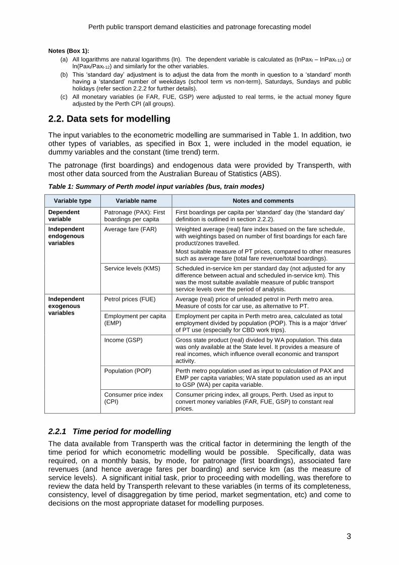
Notes (Box 1):

(a) All logarithms are natural logarithms (ln). The dependent variable is calculated as (lnPaxt – lnPaxt-12) or ln(Paxt/Paxt-12) and similarly for the other variables.

(b) This ‘standard day’ adjustment is to adjust the data from the month in question to a ‘standard’ month having a ‘standard’ number of weekdays (school term vs non-term), Saturdays, Sundays and public holidays (refer section 2.2.2 for further details).

(c) All monetary variables (ie FAR, FUE, GSP) were adjusted to real terms, ie the actual money figure adjusted by the Perth CPI (all groups).

2.2. Data sets for modelling

The input variables to the econometric modelling are summarised in Table 1. In addition, two other types of variables, as specified in Box 1, were included in the model equation, ie dummy variables and the constant (time trend) term.

The patronage (first boardings) and endogenous data were provided by Transperth, with most other data sourced from the Australian Bureau of Statistics (ABS).

Table 1: Summary of Perth model input variables (bus, train modes)

Variable type Variable name Notes and comments

Dependent variable

Patronage (PAX): First boardings per capita

First boardings per capita per ‘standard’ day (the ‘standard day’ definition is outlined in section 2.2.2).

Independent endogenous variables

Average fare (FAR) Weighted average (real) fare index based on the fare schedule, with weightings based on number of first boardings for each fare product/zones travelled.

Most suitable measure of PT prices, compared to other measures such as average fare (total fare revenue/total boardings).

Service levels (KMS) Scheduled in-service km per standard day (not adjusted for any difference between actual and scheduled in-service km). This was the most suitable available measure of public transport service levels over the period of analysis.

Independent exogenous variables

Petrol prices (FUE) Average (real) price of unleaded petrol in Perth metro area. Measure of costs for car use, as alternative to PT.

Employment per capita (EMP)

Employment per capita in Perth metro area, calculated as total employment divided by population (POP). This is a major ‘driver’ of PT use (especially for CBD work trips).

Income (GSP) Gross state product (real) divided by WA population. This data was only available at the State level. It provides a measure of real incomes, which influence overall economic and transport activity.

Population (POP) Perth metro population used as input to calculation of PAX and EMP per capita variables; WA state population used as an input to GSP (WA) per capita variable.

Consumer price index (CPI)

Consumer pricing index, all groups, Perth. Used as input to convert money variables (FAR, FUE, GSP) to constant real prices.

2.2.1 Time period for modelling

The data available from Transperth was the critical factor in determining the length of the time period for which econometric modelling would be possible. Specifically, data was required, on a monthly basis, by mode, for patronage (first boardings), associated fare revenues (and hence average fares per boarding) and service km (as the measure of service levels). A significant initial task, prior to proceeding with modelling, was therefore to review the data held by Transperth relevant to these variables (in terms of its completeness, consistency, level of disaggregation by time period, market segmentation, etc) and come to decisions on the most appropriate dataset for modelling purposes.


4

It was found that:

Up to FY 2000, the required data was available only on an annual basis.

From July 2000 onwards, the required data was available on a monthly basis, and could also be further disaggregated by passenger type (standard, concession, student), ticket type (cash, prepaid) and number of zones travelled.

From January 2009 onwards, the same data as for the earlier period was available, but now on a daily (rather than monthly) basis.

Given that the modelling required monthly (not just annual) data and also required estimation of weighted average fares, the period from July 2000 to May 2015 was selected for the econometric modelling. Use was also made of the daily data (from January 2009) to calculate day type factors which were required to determine the number of ‘standard days’ in each month.

Therefore, the main econometric modelling work was based on:

Time period July 2000 to May 2015 (ie 179 monthly data points, reducing to 167 data points when annual differences are taken).

Bus and train modes (separately).

Monthly first boardings and fare revenue data.

Aggregation of passenger types and ticket types (ie no market segmentation apart from mode), although market segment information was used to calculate weighted average fares.

2.2.2 Dependent variable

The dependent variable chosen for the modelling was total first boardings per ‘standard day’ per capita (per month, by mode).

The considerations behind this variable definition were:

First boardings. ‘First’ boardings on each ticket type was chosen, in preference to total boardings (including transfers), as it is the first boardings that directly give rise to the fare revenue.

‘Standard’ day. Monthly first boardings were expressed per ‘standard’ day, to adjust for the year-to-year variation in the number of such days in any given month. The standard day factor for any month was derived as a weighted sum of the number of days by each of the following day types in that month: weekday school term, weekday school holiday, Saturdays, Sundays and public holidays. The weightings for each day type were based on analyses of the relative first boardings by day type (by mode) from the daily patronage dataset (January 2009-May 2015).

‘Capita’. Our experience in such analyses is that population levels are highly correlated with time, and therefore that the adoption of total patronage (boardings) as the dependent variable and population as one of the independent variables results in major multi-collinearity problems. To avoid such potential problems, we chose to include population in the denominator of the dependent variable.3

2.2.3 Endogenous (independent) variables

Price variable. The price variable chosen was a weighted index of average fares (fare revenue/first boardings), with weightings proportional to the number of first boardings for each fare product/zones travelled (refer Table 1).

3 A similar approach is commonly adopted in other similar studies (eg refer work for London Transport by Mitrani et al, 2002).


5

Service (quantity and quality) variables. The service quantity variable chosen was the scheduled in-service km per ‘standard’ day4 (no adjustment was made for any differences between scheduled and actual service km operated).

The inclusion of a service quality variable was also considered, with two leadings candidates being service reliability and customer satisfaction. However, while Transperth maintains good records for both these quality aspects over most of the analysis period, consistent time series were not available because of definitional changes within the period. No quality variable was therefore included.

2.2.4 Exogenous (independent) variables

The choice of exogenous variables for inclusion in the model was relatively straightforward, with the focus being on those exogenous variables which help to ‘explain’ changes in travel behaviour and for which consistent information is available on a time-series basis over the analysis period. These choices were made in the light of:

Our knowledge of appropriate data series available from ABS.

Our previous experience from similar analyses on the key ‘drivers’ of PT patronage.

Our review of practices adopted in other similar Australasian studies (refer section 3).

The desirability of using variables for which forecasts would be available and therefore could be applied in the forecasting model.

The desirability of using variables with monthly data, given the decision to undertake modelling on a monthly basis.

Table 1 summarises the exogenous (and related) independent variables selected. This information is largely self-explanatory, but we would note in particular:

In most cases, data was available specific to the Greater Perth (GCCSA) area. This was not the case for the GSP and EMP measures, which were only available at a state-wide level: it therefore had to be assumed that the trends in GSP/capita and EMP/capita at the Perth level were identical to the equivalent trends at the state level.

In some cases (eg FUE), data was available at the required monthly level. In other cases, data was available only quarterly (GSP, EMP) or annually (POP) and monthly estimates were made by interpolation.

We also note the inclusion of a constant time trend term (𝝰 in Box 1) in the model specification. This term is intended to ‘capture’ any ‘underlying’ time trends affecting the dependent variable which are not covered by the other independent variables: omission of such a term may result in such ‘underlying’ trends being falsely attributed to another dependent variable that has some correlation with elapsed time (eg GSP).

2.3. Modelling procedures

The modelling followed an iterative process, with multiple model runs undertaken in order to arrive at the ‘best’ model for each mode. The broad approach adopted was to start with a model formulation incorporating all likely explanatory variables. Various combinations of these variables were then tested, with a view to deleting any variables that were not significant or which were highly correlated with other included variables. A selection of dummy variables was then added and the model re-run, with those variables that were significant being retained in the model. This process led to a final model formulation in which

4 The ‘standard’ day definition adopted in this case was very similar to that adopted for adjusting monthly patronage (section 2.2.2), but with day type weightings based on relative service km by day type (in place of first boardings by day type).


6

each variable had a high degree of significance, no two variables were closely correlated, and where all variables combined accounted for the highest possible proportion of the variation in the data-set (as reflected in the ‘adjusted R2 measure).

Various statistical deficiencies can undermine the validity of such econometric analyses (eg refer Kennedy 2013), with three key issues for time series analysis being:

Multi-collinearity. High correlations between explanatory variables can make econometric estimation challenging, with it being difficult to identify the relative impact on the dependent variable of two variables which are highly correlated.

Non-stationarity. A variable is regarded as ‘stationary’ if it tends to revert to a mean level over time. Regressions involving non-stationary explanatory variables can result in spurious conclusions, although in the transport economics literature non-stationary variables have often produced plausible estimates.

Endogeneity (reverse causation). Reverse causation must be taken into account, particularly in the context of changes in service levels.5

The modelling process generally resulted in elasticity estimates that were plausible (ie broadly consistency with the weight of evidence from similar analyses for the same variables elsewhere). The statistical tests undertaken were generally inconclusive and therefore some caution was seen as being desirable in applying the results of our econometric modelling directly for forecasting purposes.

Given this, our study included a review of wider Australasian evidence on demand elasticities (refer section 3), with the results being used as a check on our modelled estimates in determining the ‘best’ set of elasticity values for use for forecasting purposes for Perth.

2.4. Model results and commentary

Our modelling generally returned plausible results for both bus and train modes, as set out in Table 2. For each variable, the table shows: (i) the best (mean) elasticity estimate; (ii) the 95% confidence interval for the estimate; (iii) the statistical significance of the estimate (ie the probability of the true value being different from zero); and (iv) additional notes and comments.

We note here that the elasticity estimates derived from our modelling are essentially short-run values, reflecting market responses after around 12 months following any change in the independent variables. The issue of the most appropriate timescale for elasticity estimates is addressed in the next section.

For the model overall, the table also shows the explanatory power in terms of its adjusted R2 value. The train model in particular was found to have a relatively high explanatory power, with an adjusted R2 value of 0.82. The bus model had a much lower explanatory power, with an adjusted R2 value of 0.56: this is perhaps a somewhat disappointing result, although the individual variables almost all show high levels of significance.

5 Transperth confirmed that the great majority of bus service level changes in Perth over the analysis period were policy-driven rather than demand-driven, so we considered that reverse causation was not a major problem for our analyses.


7

Table 2: Summary of Perth preferred model elasticity results(a)

Variable Bus

(95% CI)(b)

Train (95% CI)(b) Interpretation

Average fare (FAR)

-0.38

(-0.22/-0.54)

***

-0.36

(-0.02/-0.70)

*

The fare elasticity estimates are very similar for both modes, but with the confidence interval for train being much wider than for bus. It cannot be concluded that the two estimates are significantly different from each other.

Service levels (KMS)

0.33

(0.17/0.49)

***

NA The service elasticity for bus was 0.33, with a moderate confidence interval. A service km elasticity for train could not be determined as there were no significant changes in train service levels over the analysis period (apart from Mandurah line opening).(c)

Petrol prices (FUE)

NA NA The model runs indicated that patronage was not significantly affected by changes in fuel prices.(d)


0.32

(0.11/0.53)

***

0.81

(0.42/1.19)

***

The employment (per capita) elasticity best estimates were 0.32 for bus, 0.81 train. The magnitude of these two values was broadly as expected, reflecting that a very large proportion of train users, but a much smaller proportion of bus users, are travelling to/from work.

Income (GSP) 0.26

(0.17/0.34)

***

0.28

(0.13/0.42)

***

The GSP (per capita, real terms) essentially reflects how PT use is affected by the general state of the economy. The elasticities were very similar for the two modes, and not significantly different from each other.

Annual time trend (intercept)

-0.018

(-0.013/-0.024)

***

0.001

(-0.007/0.009) n.s.

The intercept term for bus was estimated at –0.018 over the analysis period (highly significant), indicating that, after allowing for all other model factors, the ‘underlying’ trend in bus patronage/capita was a decline of some 1.8% pa. For train, the best estimate time trend per capita was extremely close to zero (in all the models tested), with a 95% confidence interval between -0.7% pa and +0.9% pa.

Adjusted R2 0.56 0.82

Notes:

(a) A number of dummy variables were used in the modelling, but are not reported in this summary of

results. Two key dummy variables were for the introduction of the student flat fare scheme in October

2005 and the opening of the Mandurah Line in Dec 2007. Dummy variables were also used to allow for

a number of outliers in the patronage data (rather than deleting the affected data points).

(b) These columns include asterisks to indicate the statistical significance of the elasticity estimates (ie the

probability of the true value being different from zero), with the following interpretation:

*** = significant at 99% level, ** = significant at 95% level, * = significant at 90% level, n.s. = not

significant (< 90%).

(c) Quite a number of the train model runs undertaken included a service km variable, but the changes in

train service km were very small and the resultant elasticity in most of these cases had a negative sign:

this is counter-intuitive, and so this variable was not included in the preferred model (indicated by NA).

The opening of the Mandurah line (represented through a dummy variable) was estimated to increase

total train system patronage by 29% within twelve months of opening.

(d) The preferred model formulation for both bus and train excludes the fuel variable because the elasticity

estimates resulting from earlier model runs were either insignificant or of the wrong (negative) sign.


8

3. Review of Australasian demand elasticity estimates

3.1. Overview – approach and relevant studies

Our experience with econometric (time series) studies of this nature into factors affecting urban PT patronage is that:

A wide range of results is found when examining individual studies. This wide range reflects several factors, including: data issues and deficiencies; differing definitions of the variables included in the model; differing modelling methodologies; wide confidence intervals; and underlying differences in market behaviour between different cities (and countries).

The range of results for the higher-quality studies tends to be much narrower than for the range of all studies, suggesting that the underlying behavioural responses are quite similar across similar market segments and situations in different cities, and that much of the apparent variation in model results across different studies and cities reflects data and methodology issues.

Most of the empirical evidence is consistent with this experience. For example, most of the higher quality studies have estimated fares elasticities of around -0.3 to -0.4; but the range of model results for all reported studies is much wider than this.

Given the evidence and this experience, our approach to estimating the most appropriate elasticity values for use in a forecasting model for Perth was not to rely on any one single econometric study, but to take a more ‘balanced’ view of the evidence not only from studies in Perth but also from studies for other cities/situations that are broadly similar. For example, we would give greater weight to high quality studies from comparable situations in other cities than we would to a low quality study for Perth. However, given that our current study has (for most variables) produced results that (i) generally have quite narrow confidence intervals; (ii) are generally consistent with the weight of evidence from other Australasian and international studies; and (iii) are generally consistent between bus and train modes (or differ in ways which are found in other studies), we placed the greatest weight on the results from our Perth study.

In pursuance of the above approach, we undertook a careful appraisal of patronage ‘drivers’ (elasticities) from previous econometric (time series) studies in Australia and New Zealand, and then compared the elasticity estimates from our Perth study with the weight of evidence from these other studies, in order to arrive at recommended elasticities for use for patronage forecasting in Perth.

Our Australasian appraisal covered ten relevant studies, all undertaken within the last 10 years: eight of these analysed Australian capital city data (of which three included Perth) and two analysed NZ data:6 bibliographic details are given in the reference section (at the end of this paper). In the following five sub-sections, for each demand ‘driver’ we provide a chart setting out the various demand elasticity estimates from the previous studies (and including our Perth study) categorised by city and mode, provide interpretation of the various results, thus leading to conclusions on the most appropriate values for use for patronage and fare revenue forecasting purposes for Perth.

We note here that elasticity values typically vary according to the timescale since the change in the relevant independent variable occurred: econometric studies often distinguish between effects in the short-run (c. 12 months after the change), the medium-run (c. 4-5 years) and the long-run (10+ years). Long-run responses are often quoted in the international literature as being around twice the short-run responses, with medium-run responses broadly midway

6 We are not aware of any evidence indicating that PT demand elasticities differ significantly between the two countries.


9

between. This study has focussed on short-run responses, on the basis that: (i) they are easier to estimate; (ii) more estimates are available from other studies; and (iii) our preferred modelling methodology (12-month difference models) provides relatively short-run estimates. While for policy analysis purposes, medium-run elasticity values could be regarded as more appropriate, some strong evidence is available in the Australasian context that, for typical bus service changes, medium-run (4-5 years) estimates are only 10%-15% greater than short-run (c. 12 months) estimates.7 This evidence is also supported for fare changes in the international context by London Transport’s econometric analyses.8

3.2. Fare levels

The Australasian evidence (from time series studies) on fare level elasticities is summarised in Figure 1: for each study this shows the best estimate and its 95% CI.9

In time series studies, fare movements are often calculated as the change in average fares, where average fares are derived as total fare revenue/total (first) boardings. Such a calculation does not allow for effects of movements between fare products: for the current study we therefore estimated fare movements based on changes in a weighted average fare index (adjusted, by CPI, to real terms).

Current study. As shown in Table 2, our Perth study short-run fare elasticity best estimate for bus was 0.38 (CI 0.22, 0.54) and for train was 0.36 (CI 0.02, 0.70).10 The CI for train was relatively wide, with that for bus being moderate, and with no evidence that the bus and train estimates are significantly different.

Other Australasian studies. Short (or short-medium) run fare elasticity estimates were identified in seven separate Australasian studies, giving 19 useful values. In relation to these studies and their values:

All but one of the 19 values relate to Australia. Most values relate to all modes combined, with only two values specific to bus.

The significant results cover a wide range, approximately 0.1 to 0.911, with the greatest concentration of values being in range 0.15 to 0.4 - which is consistent with findings elsewhere.

One of the leading Australian studies (BITRE 2013) contributes 8 of the 19 values. It gives capital city values (all PT modes) in the range 0.08 (Sydney – n.s) to 0.65 (Perth), with an unweighted average of 0.31. Even after allowing for the wide confidence intervals of the estimates, this study gives a wide range of values. In our experience, it seems most unlikely that the market responsiveness to fare changes in the eight capital cities differs as much as these results appear to indicate.12

7 Wallis IP (2013). Experience with the development of off-peak bus services. NZ Transport Agency research report 487. Wellington, New Zealand: NZ Transport Agency. https://www.nzta.govt.nz/resources/research/reports/487 8 Work reported by Mitrani et al (2002) for London Transport indicates that “85% of the total impact of a fare change occurs within a year of the change, with the final 15% of the total impact occurring over a longer period.” 9 For convenience of presentation, the signs have been reversed on all the fares elasticity estimates given in Figure 1 and the text of this section (ie the minus signs are omitted). 10 In this section and elsewhere in this paper, CI refers to the 95% confidence interval of the parameter estimate. 11 The studies covered included a number of estimates below 0.1 (which were generally not significantly different from zero). 12 We note here that, for a given dataset, studies that use annual data (as the BITRE study) result in generally less precise estimates (wider confidence intervals) than studies using quarterly or monthly data, as they have fewer data points.

https://www.nzta.govt.nz/resources/research/reports/487


10

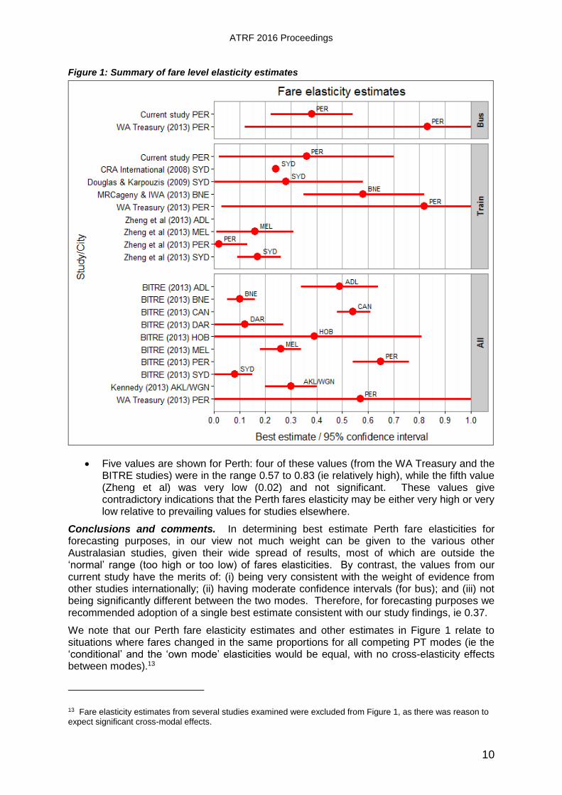
Figure 1: Summary of fare level elasticity estimates

Five values are shown for Perth: four of these values (from the WA Treasury and the BITRE studies) were in the range 0.57 to 0.83 (ie relatively high), while the fifth value (Zheng et al) was very low (0.02) and not significant. These values give contradictory indications that the Perth fares elasticity may be either very high or very low relative to prevailing values for studies elsewhere.

Conclusions and comments. In determining best estimate Perth fare elasticities for forecasting purposes, in our view not much weight can be given to the various other Australasian studies, given their wide spread of results, most of which are outside the ‘normal’ range (too high or too low) of fares elasticities. By contrast, the values from our current study have the merits of: (i) being very consistent with the weight of evidence from other studies internationally; (ii) having moderate confidence intervals (for bus); and (iii) not being significantly different between the two modes. Therefore, for forecasting purposes we recommended adoption of a single best estimate consistent with our study findings, ie 0.37.

We note that our Perth fare elasticity estimates and other estimates in Figure 1 relate to situations where fares changed in the same proportions for all competing PT modes (ie the ‘conditional’ and the ‘own mode’ elasticities would be equal, with no cross-elasticity effects between modes).13

13 Fare elasticity estimates from several studies examined were excluded from Figure 1, as there was reason to expect significant cross-modal effects.


11

We further note that all the values in Figure 1 and our recommended values relate to all-day average elasticity values. If any differential fare policies (involving different fare changes for peak and off-peak travel) were to be considered in the Perth context, we would recommend adoption of appropriate fare elasticities for the different time periods based on evidence from elsewhere (off-peak fare elasticities being typically around twice peak period elasticities).

3.3. Service levels

The Australasian evidence on service level elasticities is summarised in Figure 2. In most cases, service levels are measured as total service-kilometres (or service-hours) operated.

Figure 2: Summary of service level elasticity estimates

Current study. Our Perth study short-run best estimate elasticity for bus was 0.33 (CI 0.17, 0.49). No estimate could be made for train, as there were minimal changes in train service levels over the analysis period (apart from the introduction of the Mandurah line services, which was not an appropriate basis for estimating a standard service elasticity).

Other Australasian studies. Short-run (or short/medium-run) service level elasticity estimates were identified in four separate Australasian studies, giving 7 useful values. In relation to these studies and their values:

Six of the seven values related to Australian train services, the other value to NZ bus and train services.

Significant values covered a very wide range, between about 0.1 and 1.1. No pronounced concentration of results is evident.

For Perth, two significant previous results were available: 0.97 for train from Zheng et al/CRC study; 0.21 for bus (rail n.s.) from WA Treasury study. These two results are towards the opposite ends of the overall spectrum of results: it seems most unlikely that the real effects of service level changes are so different between Perth bus and Perth train services.

Conclusions and comments. For reasons similar to those given in regard to fare elasticities (refer section 3.2), for forecasting purposes we recommended adoption for bus mode of the best estimate from our study, ie 0.33. We also recommended adoption of this estimate for train mode, given that (i) we are not convinced by the values derived for Perth


12

from the two previous studies (and in particular the wide difference between bus and train values); (ii) the weight of international evidence does not indicate any substantial difference between bus and (urban) train service elasticities; and (iii) the 0.33 bus value from the study is broadly consistent with the weight of evidence from international studies (although perhaps somewhat on the low side).

Also, as in the case of fare elasticities, we note that if any differential fare policies were to be considered for Perth, disaggregation of the overall service elasticity value between peak and off-peak periods would be appropriate (again, with off-peak values being in the order of twice peak values).

3.4. Petrol prices

The Australasian evidence on petrol price elasticities is summarised in Figure 3. Petrol prices are generally measured as average retail petrol prices per period (e.g. month), adjusted (by CPI) to real terms.

Current study. Our Perth study was not successful in estimating any plausible petrol price elasticities. While (real) petrol prices were included in a substantial proportion of the initial modelling tests, the analyses indicated that all the resultant estimates were either not significantly different from zero or were negative (which is counter-intuitive) and apparently significant. Given this, our final model runs excluded the petrol price variable.

Other Australasian studies. Petrol price elasticity estimates were identified in six separate Australasian studies, giving 18 useful values (although some n.s.). In relation to these studies and their values:

With one exception, the results concentrated within a moderately narrow range, 0.04 to 0.25.14

In most cases, there was no clear evidence of differences between train and bus (but see further comment following).

The most detailed/disaggregated results available are for Melbourne (Currie & Phung, 2007). That study examined values by mode, trip distance and time period (peak vs off-peak). Its most pronounced finding was that values increase strongly with trip distance, with rail values being higher on average than bus values for this reason. For trips of a given distance, there was no clear evidence that rail elasticities are significantly different from (greater than?) bus elasticities, although this possibility cannot be ruled out. This variation with distance is not unexpected, given that petrol costs account for a considerably greater proportion of total trip generalised costs for longer trips. This Melbourne finding of higher elasticities (on average) for train than for bus trips is not evident in the remaining results available.

The Perth results are taken from two studies: the WA Treasury study, which gave values of 0.10 (train), 0.17 (bus) and 0.16 (overall); and the Zheng/CRC study, which gave a train value of 0.04 (but n.s). It would probably be reasonable to conclude that the Perth overall value is of similar magnitude to values elsewhere, i.e. most likely in the range 0.10 to 0.25. Based on the Melbourne data, it could be asserted that the Perth rail figure is likely to be higher than its bus figure, but there is no data other than the Melbourne evidence to support this.

14 There was also one negative result, and most of the results between zero and 0.1 were not significant.


13

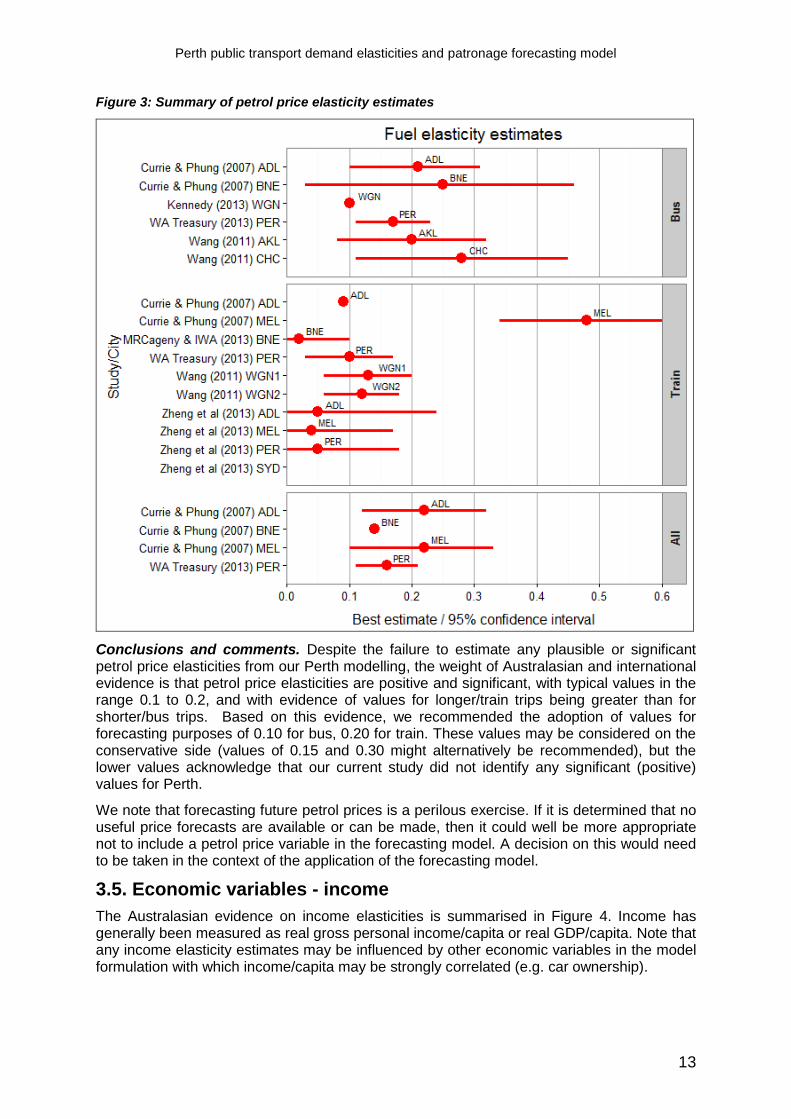
Figure 3: Summary of petrol price elasticity estimates

Conclusions and comments. Despite the failure to estimate any plausible or significant petrol price elasticities from our Perth modelling, the weight of Australasian and international evidence is that petrol price elasticities are positive and significant, with typical values in the range 0.1 to 0.2, and with evidence of values for longer/train trips being greater than for shorter/bus trips. Based on this evidence, we recommended the adoption of values for forecasting purposes of 0.10 for bus, 0.20 for train. These values may be considered on the conservative side (values of 0.15 and 0.30 might alternatively be recommended), but the lower values acknowledge that our current study did not identify any significant (positive) values for Perth.

We note that forecasting future petrol prices is a perilous exercise. If it is determined that no useful price forecasts are available or can be made, then it could well be more appropriate not to include a petrol price variable in the forecasting model. A decision on this would need to be taken in the context of the application of the forecasting model.

3.5. Economic variables - income

The Australasian evidence on income elasticities is summarised in Figure 4. Income has generally been measured as real gross personal income/capita or real GDP/capita. Note that any income elasticity estimates may be influenced by other economic variables in the model formulation with which income/capita may be strongly correlated (e.g. car ownership).


14

Figure 4: Summary of income elasticity estimates

Current study. Our Perth study short-run elasticity estimates for GSP (a proxy for real household incomes) per capita were bus 0.26 (CI 0.17, 0.34) and train 0.28 (CI 0.13, 0.42).

Other Australasian studies. Income elasticity estimates were identified in five separate Australasian studies, giving 15 useful values. In relation to these studies and their values:

All these studies used real gross income per capita, or a similar measure. 15

Values (best estimates) varied over a wide range, -0.44 to +1.61. 11 of the 15 values were between 0.0 and 1.0, with eight being between 0.2 and 0.8, the median being around 0.5.

The expectation would be that income elasticity values would depend on what other economic variables were included in the model formulation. For three of the five studies, the models included either employment level or car ownership, both of which would be likely to be strongly (positively) correlated with income.

Where car ownership is included separately, then the residual income effect seems likely to be modestly positive; whereas otherwise the combined income/car ownership effect is likely to be negative. If employment is included in the model

15 The BITRE (2013) study used a ‘disposable income constraint’ (refer study report for details).


15

formulation, the likely effects are less clear: higher incomes will tend to be correlated with higher employment, which would tend to increase PT use (additional commuter trips), but also tend to reduce PT travel as a result of higher car ownership. The overall effects are unclear. The very limited evidence from the studies reviewed does not clearly confirm (or deny) the hypothesis about the effects of including car ownership separately.16

Conclusions and comments. We consider that the estimates derived in our current study (which are significantly positive but relatively low) are plausible, noting that: (i) the employment variable was included separately in the analysis; (ii) the estimates refer to the short/medium term perspective; (iii) car ownership effects are unlikely to be substantial over the analysis period; and (iv) the bus and train best estimates are almost identical, with the confidence intervals being reasonably narrow. We therefore recommended that a system-wide income elasticity value of 0.27 be applied for forecasting purposes.

3.6. Economic variables - employment

The Australasian evidence on employment elasticities is summarised in Figure 5. In the four studies analysed, the employment variable has been measured variously as the total number of people employed, total office employment, or total employment per capita. Our preference has been to adopt the employment per capita measure, as this is consistent with our definition of the dependent variable and separates out the effects of population changes from the effects of changes in employment rates. Typically, with rising population and rising employment rates, the per capita approach will tend to result in higher elasticity estimates than the total population approach.

Current study. Our Perth study estimated elasticities for employment/capita of bus 0.32 (CI 0.11, 0.53) and train 0.81 (CI 0.42, 1.19). The absolute and relative magnitudes of these bus and train estimates are broadly as expected, reflecting that a very large proportion of train usage but a much smaller proportion of bus usage is for trips to/from work.

Other Australasian studies. Employment elasticities were estimated in four separate Australasian studies (six values in total), with three of these studies using a total employment variable and one an employment/capita variable. In relation to these studies and their values:

The various elasticity estimates varied from about 0.4 to 1.4, generally with wide confidence intervals. Four of the six values related to train mode and these showed a tendency to be higher than the values for bus mode (although the samples involved are very small). There was no clear evidence that the elasticity estimates on a per capita basis differed from those on a total population basis.

Various NZ evidence (not reflected in figure 5) indicates that peak period train elasticities with respect to employment are two to three times the corresponding bus elasticities: this is consistent with our study’s relative values for train and bus.

Conclusions and comments. Given the limitations of the other Australasian studies on employment elasticities (ie the limited evidence, the wide spread of estimates (with wide CIs) and the differing definitions used) along with the reasonableness of our study estimates (in both absolute and relative terms), we recommended the adoption of our best estimate employment/capita elasticities (0.32 for bus, 0.81 for train) for forecasting purposes.

16 We note that the TRL ‘Demand for Public Transport’ report (Balcombe et al, 2004) suggests that overall

income elasticities are likely to be negative for bus use, but positive for train use (although this train conclusion may relate primarily to longer-distance rather than urban train travel.


16

Figure 5: Summary of employment elasticity estimates

3.7. Proposed elasticity values for forecasting

A summary of the recommended elasticity values for use in the forecasting model, drawing on the previous sub-sections, is given in Table 3.

Table 3: Recommended elasticity values for use in forecasting model

Item Definition

Recommended best estimates Interpretation

Bus Train

Patronage/ capita (PAX)

First boardings per capita per ‘standard’ day

Dependent variable.

Average fare (FAR)

Fare revenue (real) per first boarding (based on fare index approach)

-0.37 Average of our separate Perth bus and train results (not significantly different).

Service levels (KMS)

Scheduled in-service km per standard day

0.33

Based on our study results for bus (not possible to establish separate train value, but no evidence from elsewhere of significant modal differences)

Petrol prices (FUE)

Average real price of unleaded petrol in Perth metro area. 0.10 0.20

Based on weight of Australasian (and international) evidence (our study did not find significant effects).


Employment per capita in Perth metro area 0.32 0.81

Forecast figures taken directly from our study estimates.

Income (GSP) Gross state product (real terms) divided by WA population.

0.27 Average of separate Perth bus and train results (not significantly different).

‘Underlying’ time trend

Constant time trend over the analysis period (not explained by other factors)

-0.018 (-1.8%

pa) 0.00

No reason to change estimates from our study’s econometric analysis results.(a)

Note: (a) Our review of demand elasticities from other Australasian studies did not specifically examine

evidence on ‘underlying’ time trends; but we are aware from previous econometric/time series studies that time trends (per capita) between zero and -2% pa are typical.


17

4. Perth patronage forecasting model

4.1. Model requirements

From the perspective of our client (Transperth), the key output of the consultancy assignment was the provision of a model for forecasting future patronage (first boardings) and associated fare revenue for Perth’s bus and train services: the model was required to provide updated patronage and revenue forecasts on an ongoing basis as inputs to Transperth’s planning and budgeting functions and also to support financial negotiations with the WA Government.

The forecasting model developed was structured along very similar lines to the time series analysis model outlined earlier (section 2), with the elasticity estimates derived from the earlier work (Table 3) now being applied as inputs to the forecasting process. Given this similarity of approach, only brief details of the model formulation are provided in this section.

4.2. Model structure, inputs, outputs and application procedures

4.2.1. Model structure

As for the time series analysis, the forecasting model was structured as a 12-month difference model, ie the patronage (first boardings) in any month is estimated by starting from the patronage in the corresponding month in the previous year and then for each causal variable applying factors for: (i) the proportional change in the variable, multiplied by (ii) the estimated demand elasticity with respect to that variable.

The mathematical formulation for the forecasting model essentially follows the specification in Box 1 (but excluding any dummy variables) and applies the elasticity values from Table 3.

The starting point (‘base year’) adopted for the modelling process would usually be the most recent financial year for which full actual patronage data is available (although the model user may choose any 12-month period, subject to data availability).

4.2.2. Model inputs

The key inputs to the model are in four main categories:

‘Base year’ statistics by month (and by mode as appropriate) relating to first boardings and fare revenue, endogenous (fares and service levels) inputs and exogenous (demographic and economic) inputs.

Future estimates (monthly/quarterly/yearly) of the key ‘drivers’ influencing patronage, covering endogenous variables (principally fare levels and service km) and various exogenous (economic and demographic) variables (refer Table 1).17

Demand elasticities (as in Table 3), expressing the relationships established between proportionate changes in the key ‘driver’ variables and proportionate changes in patronage.

Future holiday and school term dates, to enable the number of ‘standard days’ per month to be calculated throughout the forecasting period (refer Table 1 and section 2.2.2).

4.2.3. Model outputs and application

With application of the above inputs, the model first estimates total first boardings per capita per standard day for each mode (bus and train) on a monthly basis. The final required forecast outputs of total first boardings and total fare revenue by month are then derived by applying the following month-specific factors:

17 Forecasts for all the exogenous variables for a 4-year period were available from WA Treasury


18

Number of ‘standard days’ (DAYS-PAX), by mode

Greater Perth estimate of normally resident population (POP) for the relevant month

Weighted average fare by mode (to convert first boardings into fare revenue).

The forecasting model was developed so as to be relatively simple and quick to apply:

It is Excel-based (including in the Excel workbook further instructions and advice to guide model users on input requirements).

For the ‘base’ year, actual values by month by mode are entered into the model spreadsheet for all the specified input variables. For the future (forecast) years, forecast values by month by mode are required for the Independent variables.

In practice, most variables (POP, EMP, INCOME and CPI) require only an annual forecast (as at June each year), with monthly values interpolated by the model. The other variables use monthly or quarterly forecasts, but only require forecast values to be input for those months in which they change. Further, for simplicity (and to minimise the chance of errors), most of the forecast inputs are entered as percentage changes from the variable value 12 months earlier.

The model may (in principle) be applied for as many years into the future as required, but subject to the availability of forecasts for the required model inputs. The level of confidence that may be placed on model forecast outputs is dependent on the confidence in the forecasts for the various input variables (as well as the model elasticity values). In practice, we suggest that the model should not usually be applied for forecasting more than 3-4 years ahead, and that sensitivity testing on forecasts for key variable should be undertaken.

4.2.4. Model testing and example results

As part of model ‘proving’ prior to hand-over to our client, we applied the model to several scenarios specified in terms of future movements in each of the endogenous and exogenous variables over the 5-year period to 2020. While the model test results are not given here, findings of interest include:

Metropolitan area population growth is expected to be one of the main factors affecting patronage over the 5-year period, with population growth and resultant patronage growth approaching 10%.

The estimated ‘underlying’ time trend (-1.8% pa for bus, zero for train) is the dominant factor leading to higher patronage growth for train than for the bus system.

Given the forecasts (from WA Treasury) of low inflation over the period, the effects on patronage of keeping fares constant in money terms (relative to fares being adjusted for inflation) would be modest, only about 4% by 2020.

Arguably the greatest uncertainty relating to the impacts of the exogenous variables on future patronage relates to petrol prices, which have historically been relatively ‘volatile’ (and even though the cross-elasticity of patronage with respect to petrol prices is relatively low).

5. Conclusions

The work described in this paper was undertaken to assist Transperth in its planning and budgeting functions, and also to support its annual financial negotiations with the WA Government, particularly in relation to potential changes in fare levels and structures.

We consider that the project has been successful in meeting its objectives. Besides providing improved understanding of the factors that have influenced patronage changes in Perth over the last 15 years, the project has developed and incorporated into the forecasting model a set of demand elasticity estimates that: (i) are closely based on the results of our


19

econometric analyses of past patronage changes in Perth; (ii) take account of elasticity evidence from other similar econometric studies for Australasian cities; and (iii) have regard to, and are generally consistent with, wider international evidence on the patronage ‘drivers’ for metropolitan public transport services.

Our experience in the project of econometric analysis of Perth’s past patronage changes has reinforced our views about the difficulties likely to arise in such analyses, and the sensitivity of modelling results (elasticity estimates etc) to data inputs, model formulation and statistical issues. A substantial proportion of the project consulting resources was involved in developing a ‘clean’ data set suitable for analysis.

Our review of other Australasian econometric analyses of public transport patronage time series data further illustrates the difficulties often encountered in deriving ‘good’ and consistent elasticity estimates. The most pronounced characteristic of the 10 Australian studies reviewed was the wide spread of elasticity estimates for each variable of interest. In our view, this wide spread does not indicate that underlying behavioural responses are very different in different cities, but rather reflects the difficulties inherent in such analyses (associated with data issues, modelling methods, definitions of variables etc). We are of the view that the underlying behavioural responses to the various endogenous and exogenous factors are generally very similar (for comparable market segments) in different cities -- certainly within Australasia and, to a large extent, in other developed countries.

While, in our view, the project has been generally successful, in particular in terms of the forecasting model delivered to our client, we suggest that future improvements would be desirable in a number of aspects (time, budget and data permitting), including:

The inclusion in the model of one or more service quality variables. Leading candidates in the Perth case would be overall customer satisfaction (or a subset of this) and service reliability - both of which are known to be significant determinants of market behaviour.

The inclusion of variables relating specifically to CBD employment levels (rather than metropolitan employment generally) and to CBD parking supply and/or pricing. (There would seem little doubt that the CBD parking restraint policies adopted in Perth over a number of years have had a significant impact on public transport’s market share for CBD trips, which is not directly reflected in the current model.)

The estimation of medium-run (say 4-5 years) elasticity values as well as short-run values. We gave this lower priority in the project, recognising the greater econometric challenges involved and the evidence that medium-run elasticities are not a lot greater than (typically within c. 20% of) short-run values.

Subject to these caveats, and based on the view that underlying market behaviour is very similar in different cities (certainly within Australasia), we consider that application of the Perth model to other cities, with relatively minor changes at least initially, could provide valuable insights into the major factors likely to influence their future patronage trends and the strength of these influences.

6. Acknowledgements

This paper is based on a consultancy assignment undertaken by Ian Wallis Associates Ltd for Transperth, a division of the WA Public Transport Authority. The authors wish to thank Ian Vinicombe and Brendan Lumbers of Transperth for their support throughout this assignment and in publication of this paper.


20

7. References18

Balcombe R (editor) et al (2004) The demand for public transport; a practical guide. Crowthorne: TRL Ltd.

*BITRE (2013) Public transport use in Australia’s capital cities: Modelling and forecasting. Report 129. Canberra, Australia: Bureau of Infrastructure, Transport and Regional Economics. https://bitre.gov.au/publications/2013/report_129.aspx

*CRA International (2008) Value of CityRail externalities and optimal Government Subsidy. Final Report. IPART. http://www.ipart.nsw.gov.au/files/sharedassets/website/trimholdingbay/crai_report_-_cityrail_externalities_-_6_june_2008.pdf

*Currie, G and J Phung (2007) Aggregate and disaggregate analysis of fuel price impacts on public transport demand. Australasian Transport Research Forum 2007.

*Douglas, N and G Karpouzis (2009) An explorative econometric model of Sydney metropolitan rail patronage. Australasian Transport Research Forum 2009. http://www.patrec.org/web_docs/atrf/papers/2009/1799_paper195-Douglas.pdf

Ian Wallis Associates Ltd (2016) Perth patronage analysis and forecasting project: main report. Report to Transperth/WA Public Transport Authority.

*Kennedy, D (2013) Econometric models for public transport forecasting March 2013. NZ Transport Agency research report 518. Wellington, New Zealand: NZ Transport Agency. https://www.nzta.govt.nz/resources/research/reports/518/

*MRCagney and Ian Wallis Associates (2013) SEQ fare path strategy – Analysis of rail system elasticities Draft Report.

Mitrani et al (2002) London transport traffic trends: London underground and bus demand analysis 1970 - 2000.

*Odgers, JF and LA van Schijndel (2011) Forecasting annual train boardings in Melbourne using time series data. Australasian Transport Research Forum 2011. http://atrf.info/papers/2011/2011_Odgers_vanSchijndel.pdf

*WA Treasury (2013) A Preliminary Assessment of Public Transport Patronage in Perth. Perth, Australia: Government of Western Australia, Department of Treasury.

Wallis IP (2013). Experience with the development of off-peak bus services. NZ Transport Agency research report 487. Wellington, New Zealand: NZ Transport Agency. https://www.nzta.govt.nz/resources/research/reports/487

*Wang, J (2011) Appraisal of factors influencing public transport patronage. NZ Transport Agency research report 434. Wellington, New Zealand: NZ Transport Agency. https://www.nzta.govt.nz/resources/research/reports/434/

*Zheng, Z, Wijeweera, A, Charles, M et al (2013) Understanding urban rail travel for improved patronage forecasting. Brisbane, Qld: CRC for Rail Innovation. http://eprints.qut.edu.au/94978/

18 References marked * are those from which Australasian elasticity estimates were taken (refer section 3 of this

paper).

https://bitre.gov.au/publications/2013/report_129.aspx

http://www.ipart.nsw.gov.au/files/sharedassets/website/trimholdingbay/crai_report_-_cityrail_externalities_-_6_june_2008.pdf

http://www.ipart.nsw.gov.au/files/sharedassets/website/trimholdingbay/crai_report_-_cityrail_externalities_-_6_june_2008.pdf

http://www.patrec.org/web_docs/atrf/papers/2009/1799_paper195-Douglas.pdf

https://www.nzta.govt.nz/resources/research/reports/518/

http://atrf.info/papers/2011/2011_Odgers_vanSchijndel.pdf

https://www.nzta.govt.nz/resources/research/reports/487

https://www.nzta.govt.nz/resources/research/reports/434/

http://eprints.qut.edu.au/94978/

forecasting perth’s public transport patronage: … 2016 proceedings 1 forecasting perth’s...

Documents